algorithms - dei.unipd.itmusica/im06/dispense06/8_algorithms_parte1.pdf · algorithms figure 7.1:...

Chapter 7

Algorithms

version 14th November 2005

7.1 Markov Models and Hidden Markov Models

Andrei Andreevich Markov first introduced his mathematical model of dependence, now known asMarkov chains, in 1907. A Markov model (or Markov chain) is a mathematical model used to rep-resent the tendency of one event to follow another event, or even to follow an entire sequence ofevents. Markov chains are matrices comprised of probabilities that reflect the dependence of one ormore events on previous events. Markov first applied his modeling technique to determine tendenciesfound in Russian spelling. Since then, Markov chains have been used as a modeling technique for awide variety of applications ranging from weather systems to baseball games.

Statistical methods of Markov source or hidden Markov modeling (HMM) have become increas-ingly popular in the last several years. The models are very rich in mathematical structure and hencecan form a basis for use in a wide range of applications. Moreover the models, when applied properly,work very well in practice for several important applications.

7.1.1 Markov Models or Markov chains

Markov models are very useful to represent families of sequences with certain specific statisticalproperties. To explain the idea consider a simple 3 state model of the weather. We assume that oncea day, the weather is observed as being one of the following: rain (state 1); cloudy (state 2); sunny(state 3).

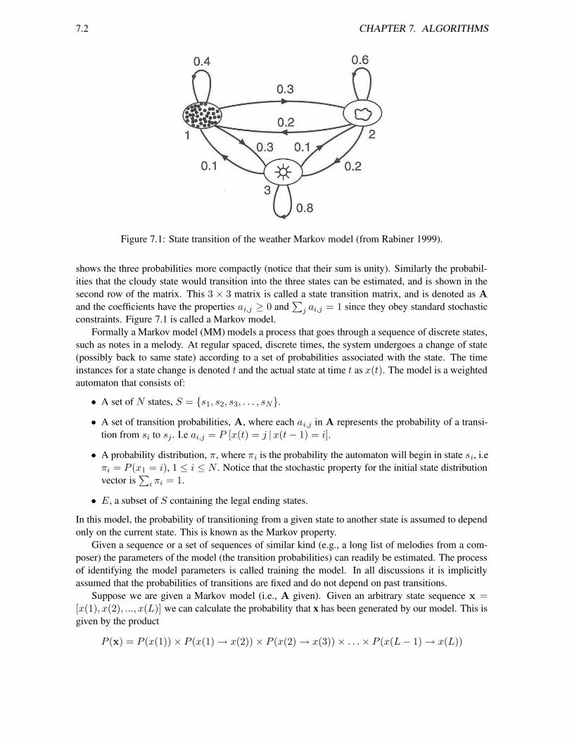
If we examine a sequence of observation during a month, the state rain appears a few times, andit can be followed by rain, cloud or sun. Given a long sequence of observations, we can count thenumber of times the state rain is followed by, say, a cloudy state. From this we can estimate theprobability that a rain is followed by a cloudy state. If this probability is 0.3 for example, we indicateit as shown in Figure 7.1. The figure also shows examples of probabilities for every state to transitionto other states, including itself. The first row of the matrix A

A = {ai,j} =

0.4 0.3 0.30.2 0.6 0.20.1 0.1 0.8

(7.1)

7.1

7.2 CHAPTER 7. ALGORITHMS

Figure 7.1: State transition of the weather Markov model (from Rabiner 1999).

shows the three probabilities more compactly (notice that their sum is unity). Similarly the probabil-ities that the cloudy state would transition into the three states can be estimated, and is shown in thesecond row of the matrix. This 3 × 3 matrix is called a state transition matrix, and is denoted as A

and the coefficients have the properties ai,j ≥ 0 and∑

j ai,j = 1 since they obey standard stochasticconstraints. Figure 7.1 is called a Markov model.

Formally a Markov model (MM) models a process that goes through a sequence of discrete states,such as notes in a melody. At regular spaced, discrete times, the system undergoes a change of state(possibly back to same state) according to a set of probabilities associated with the state. The timeinstances for a state change is denoted t and the actual state at time t as x(t). The model is a weightedautomaton that consists of:

• A set of N states, S = {s1, s2, s3, . . . , sN}.

• A set of transition probabilities, A, where each ai,j in A represents the probability of a transi-tion from si to sj . I.e ai,j = P [x(t) = j |x(t− 1) = i].

• A probability distribution, π, where πi is the probability the automaton will begin in state si, i.eπi = P (x1 = i), 1 ≤ i ≤ N . Notice that the stochastic property for the initial state distributionvector is

∑

i πi = 1.

• E, a subset of S containing the legal ending states.

In this model, the probability of transitioning from a given state to another state is assumed to dependonly on the current state. This is known as the Markov property.

Given a sequence or a set of sequences of similar kind (e.g., a long list of melodies from a com-poser) the parameters of the model (the transition probabilities) can readily be estimated. The processof identifying the model parameters is called training the model. In all discussions it is implicitlyassumed that the probabilities of transitions are fixed and do not depend on past transitions.

Suppose we are given a Markov model (i.e., A given). Given an arbitrary state sequence x =[x(1), x(2), ..., x(L)] we can calculate the probability that x has been generated by our model. This isgiven by the product

P (x) = P (x(1)) × P (x(1) → x(2)) × P (x(2) → x(3)) × . . .× P (x(L− 1) → x(L))

7.1. MARKOV MODELS AND HIDDEN MARKOV MODELS 7.3

where P (x(1)) = π(x(1)) is the probability that x(1) is the initial state, P (x(k) → x(m)) is thetransition probability for going from x(k) to x(m), and can be found from the matrix A. For examplewith reference to the weather Markov model of equation 7.1, given that the weather on day 1 is sunny(state 3), we can ask the question: What is the probability that the weather for next 7 days will be”sun-sun-rai-rain-sun-cloudy-sun . .”? This probability can be evaluated as

P = π3 · a33 · a33 · a31 · a11 · a13 · a32 · a13

= 1(0.8)(0.8)(0.1)(0.4)(0.3)(0.1)(0.2)

= 1.536 × 10−4

The usefulness of such computation is as follows: given a number of Markov models (A1 fora composer, A2 for a second composer, and so forth) and given a melody x, we can calculate theprobabilities that this melody is generated by any of these models. The model which gives the highestprobability is most likely the model which generated the sequence.

7.1.2 Hidden Markov Models

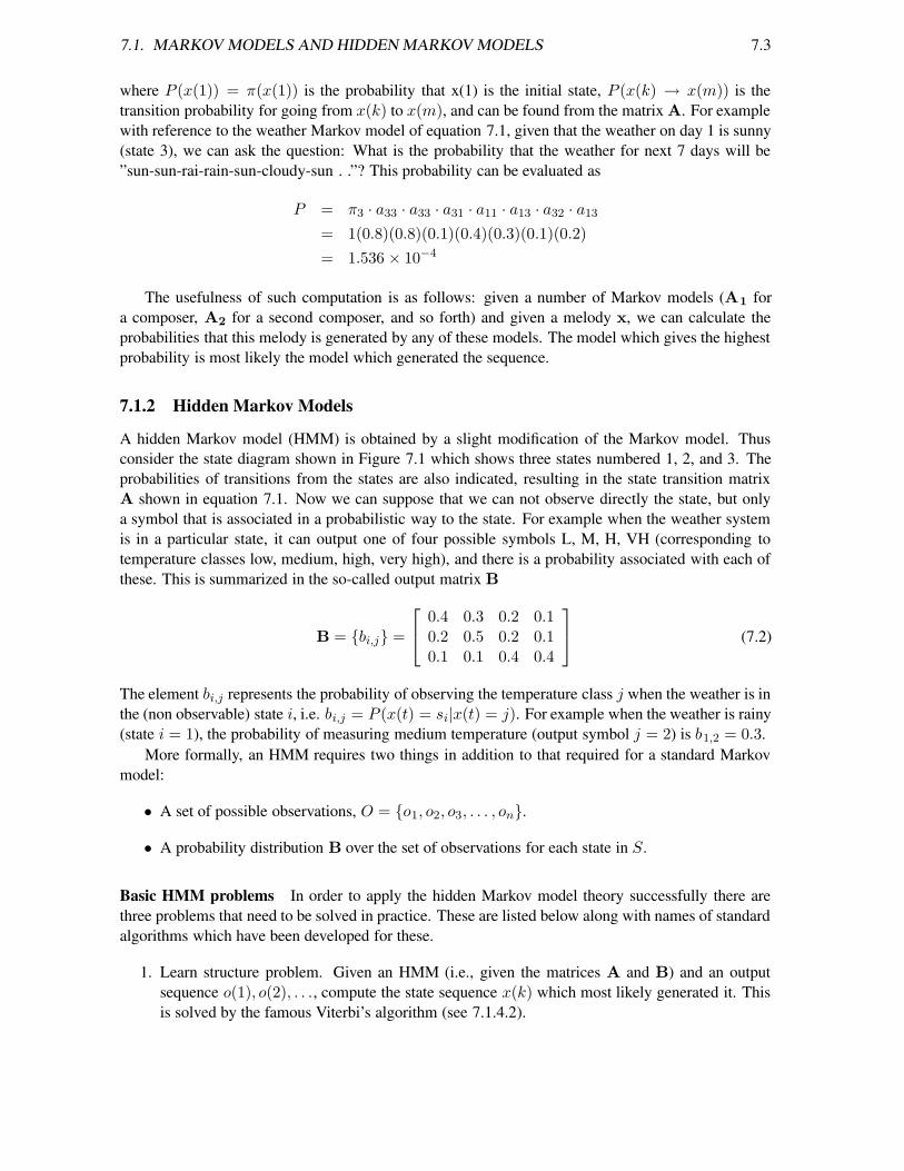
A hidden Markov model (HMM) is obtained by a slight modification of the Markov model. Thusconsider the state diagram shown in Figure 7.1 which shows three states numbered 1, 2, and 3. Theprobabilities of transitions from the states are also indicated, resulting in the state transition matrixA shown in equation 7.1. Now we can suppose that we can not observe directly the state, but onlya symbol that is associated in a probabilistic way to the state. For example when the weather systemis in a particular state, it can output one of four possible symbols L, M, H, VH (corresponding totemperature classes low, medium, high, very high), and there is a probability associated with each ofthese. This is summarized in the so-called output matrix B

B = {bi,j} =

0.4 0.3 0.2 0.10.2 0.5 0.2 0.10.1 0.1 0.4 0.4

(7.2)

The element bi,j represents the probability of observing the temperature class j when the weather is inthe (non observable) state i, i.e. bi,j = P (x(t) = si|x(t) = j). For example when the weather is rainy(state i = 1), the probability of measuring medium temperature (output symbol j = 2) is b1,2 = 0.3.

More formally, an HMM requires two things in addition to that required for a standard Markovmodel:

• A set of possible observations, O = {o1, o2, o3, . . . , on}.

• A probability distribution B over the set of observations for each state in S.

Basic HMM problems In order to apply the hidden Markov model theory successfully there arethree problems that need to be solved in practice. These are listed below along with names of standardalgorithms which have been developed for these.

1. Learn structure problem. Given an HMM (i.e., given the matrices A and B) and an outputsequence o(1), o(2), . . ., compute the state sequence x(k) which most likely generated it. Thisis solved by the famous Viterbi’s algorithm (see 7.1.4.2).


2. Evaluation or scoring problem. Given the HMM and an output sequence o(1), o(2), . . . computethe probability that the HMM generates this. We can also view the problem as one of scoringhow well a given model matches a given output sequence. If we are trying to choose amongseveral competing models, this ranking allow us to choose the model that best matches theobservations. The forward-backward algorithm solves this (see 7.1.4.1).

3. Training problem. How should one design the model parameters A and B such that they areoptimal for an application, e.g., to represent a melody? The most popular algorithm for this isthe expectation maximization algorithm commonly known as the EM algorithm or the Baum-Welch algorithm (see [2] for more details).

Figure 7.2: Block diagram of an isolated word recognizer (from Rabiner 1999).

For example let us consider a simple isolated word recognizer (see Figure 7.2). For each word wewant to design a separate N -state HHM. We represent the speech signal as a time sequence of codedspectral vectors. Hence each observation is the index of the spectral vector closest to the originalspeech signal. Thus for each word, we have a training sequence consisting of repetitions of codebookindices of the word.

The first task is to build individual word models. This task is done by using the solution to Prob-lem 3 to estimate model parameters for each word model. To develop an understanding of physicalmeaning of the model state, we use the solution to Problem 1 to segment each of the word state se-quence into states, and then study the properties of the spectral vectors that lead to the observationsoccurring in each state. Finally, once the set of HMMs has been designed, recognition of an unknownword is performed using the solution to Problem 2 to score each word model based on the observationsequence, and select the word whose model score is highest.

We should remark that the HMM is a stochastic approach which models the given problem as adoubly stochastic process in which the observed data are thought to be the result of having passed thetrue (hidden) process through a second process. Both processes are to be characterized using onlythe one that could be observed. The problem with this approach, is that one do not know anythingabout the Markov chains that generate the speech. The number of states in the model is unknown,


there probabilistic functions are unknown and one can not tell from which state an observation wasproduced. These properties are hidden, and thereby the name hidden Markov model.

7.1.3 Markov Models Applied to Music

Hiller and Isaacson (1957) were the first to implement Markov chains in a musical application. Theydeveloped a computer program that used Markov chains to compose a string quartet comprised of fourmovements entitled the Illiac Suite. Around the same time period, Meyer and Xenakis (1971) realizedthat Markov chains could reasonably represent musical events. In his book Formalized Music [4],Xenakis described musical events in terms of three components: frequency, duration, and intensity.These three components were combined in the form of a vector and then were used as the states inMarkov chains. In congruence with Xenakis, Jones (1981) suggested the use of vectors to describenotes (e.g., note = pitch, duration, amplitude, instrument) for the purposes of eliciting more complexmusical behavior from a Markov chain. In addition, Polansky, Rosenboom, and Burk (1987) proposedthe use of hierarchical Markov chains to generate different levels of musical organization (e.g., a highlevel chain to define the key or tempo, an intermediate level chain to select a phrase of notes, and alow level chain to determine the specific pitches). All of the aforementioned research deals with thecompositional aspects and uses of Markov chains. That is, all of this research was focused on creatingmusical output using Markov chains.

7.1.3.1 HMM models for music search: MuseArt

In the MuseArt system for music search and retrieval, developed at Michigan University by JonahShifrin, Bryan Pardo, Colin Meek, William Birmingham, musical themes are represented using ahidden Markov model (HMM).

Representation of a query. The query is treated as an observation sequence and a theme is judgedsimilar to the query if the associated HMM has a high likelihood of generating the query. A piece ofmusic is deemed a good match if at least one theme from that piece is similar to the query. The piecesare returned to the user in order, ranked by similarity.

Figure 7.3: A sung query (from Shifrin 2002)


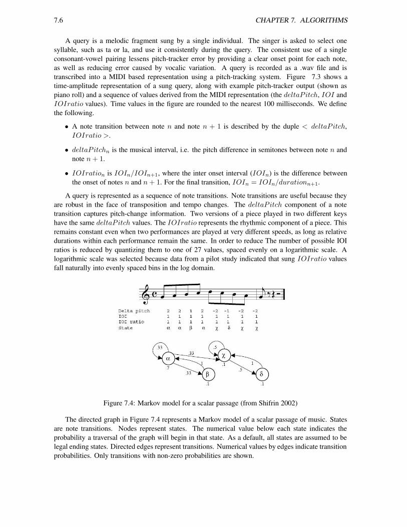
A query is a melodic fragment sung by a single individual. The singer is asked to select onesyllable, such as ta or la, and use it consistently during the query. The consistent use of a singleconsonant-vowel pairing lessens pitch-tracker error by providing a clear onset point for each note,as well as reducing error caused by vocalic variation. A query is recorded as a .wav file and istranscribed into a MIDI based representation using a pitch-tracking system. Figure 7.3 shows atime-amplitude representation of a sung query, along with example pitch-tracker output (shown aspiano roll) and a sequence of values derived from the MIDI representation (the deltaP itch, IOI andIOIratio values). Time values in the figure are rounded to the nearest 100 milliseconds. We definethe following.

• A note transition between note n and note n + 1 is described by the duple < deltaP itch,IOIratio >.

• deltaP itchn is the musical interval, i.e. the pitch difference in semitones between note n andnote n+ 1.

• IOIration is IOIn/IOIn+1, where the inter onset interval (IOIn) is the difference betweenthe onset of notes n and n+ 1. For the final transition, IOIn = IOIn/durationn+1.

A query is represented as a sequence of note transitions. Note transitions are useful because theyare robust in the face of transposition and tempo changes. The deltaP itch component of a notetransition captures pitch-change information. Two versions of a piece played in two different keyshave the same deltaP itch values. The IOIratio represents the rhythmic component of a piece. Thisremains constant even when two performances are played at very different speeds, as long as relativedurations within each performance remain the same. In order to reduce The number of possible IOIratios is reduced by quantizing them to one of 27 values, spaced evenly on a logarithmic scale. Alogarithmic scale was selected because data from a pilot study indicated that sung IOIratio valuesfall naturally into evenly spaced bins in the log domain.

Figure 7.4: Markov model for a scalar passage (from Shifrin 2002)

The directed graph in Figure 7.4 represents a Markov model of a scalar passage of music. Statesare note transitions. Nodes represent states. The numerical value below each state indicates theprobability a traversal of the graph will begin in that state. As a default, all states are assumed to belegal ending states. Directed edges represent transitions. Numerical values by edges indicate transitionprobabilities. Only transitions with non-zero probabilities are shown.


In Markov model, it is implicitly assumed that whenever state s is reached, it is directly observable,with no chance for error. This is often not a realistic assumption. There are multiple possible sourcesof error in generating a query. The singer may have incorrect recall of the melody he or she isattempting to sing. There may be production errors (e.g., cracked notes, poor pitch control). Thetranscription system may introduce pitch errors, such as octave displacement, or timing errors due tothe quantization of time. Such errors can be handled gracefully if a probability distribution over the setof possible observations (such as note transitions in a query) given a state (the intended note transitionof the singer) is maintained. Thus, to take into account these various types of errors, the Markovmodel should be extended to a hidden Markov Model, or HMM. The HMM allows us a probabilisticmap of observed states to states internal to the model (hidden states). In the system, a query is asequence of observations. Each observation is a note-transition duple, < deltaP itch, IOIratio >.Musical themes are represented as hidden Markov models whose states also corresponds to note-transition duples. To make use of the strengths of a hidden Markov model, it is important to modelthe probability of each observation oi in the set of possible observations, O, given a hidden state, s.

Making Markov Models from MIDI. Our system represents musical themes in a database asHMMs. Each HMM is built automatically from a MIDI file encoding the theme. The unique duplescharacterizing the note transitions found in the MIDI file form the states in the model. FigureFig-ure 7.4 shows a passage with eight note transitions characterized by four unique duples. Each uniqueduple is represented as a state. Once the states are determined for the model, transition probabilitiesbetween states are computed by calculating what proportion of the time state a follows state b in thetheme. Often, this results in a large number of deterministic transitions. Figure 7.5 is an exampleof this, where only a single state has two possible transitions, one back to itself and the other on tothe next state. Note that there is not a one-to-one correspondence between model and observation se-

Figure 7.5: Markov model for Alouette fragment (from Shifrin 2002)

quence. A single model may create a variety of observation sequences, and an observation sequencemay be generated by more than one model. Recall that our approach defines an observation as a du-ple, ¡deltaPitch, IOIratio¿. Given this, the observation sequence q = {(2, 1), (2, 1), (2, 1)} may begenerated by the HMM in Figure 7.4 or the HMM in Figure 7.5.

Finding the best target. The themes in the database are coded as HMMs and the query is treated asan observation sequence. Given this, we are interested in finding the HMM most likely to generate theobservation sequence. This can be done using the Forward algorithm. The Forward algorithm, given


an HMM and an observation sequence, returns a value between 0 and 1, indicating the probability theHMM generated the observation sequence. Given a maximum path length, L, the algorithm takes allpaths through the model of up to L steps. The probability each path has of generating the observationsequence is calculated and the sum of these probabilities gives the probability that the model generatedthe observation sequence. This algorithm takes on the order of |S|2L steps to compute the probability,where |S| is the number of states in the model.

Let there be an observation sequence (query), O, and a set of models (themes), M . An order maybe imposed on M by performing the Forward algorithm on each model m in M and then ordering theset by the value returned, placing higher values before lower. The i-th model in the ordered set is thenthe i-th most likely to have generated the observation sequence. We take this rank order to be a directmeasure of the relative similarity between a theme and a query. Thus, the first theme is the one mostsimilar to the query.

7.1.3.2 Markov sequence generator

Markov models can be thought of as generative models. A generative model describes an underlyingstructure able to generate the sequence of observed events, called an observation sequence. Note thatthere is not a one-to-one correspondence between model and observation sequence. A single modelmay create a variety of observation sequences, and an observation sequence may be generated bymore than one model.

A HMM can be used as generator to give an observation sequence O as follow

1. Choose initial state x(1) = S1 according the initial state distribution π.

2. Set t = 1

3. Choose o(t) according the symbol probability distribution in state x(t) described in matrix B

4. Transit to new state x(t+1) = Sj according to the state transition probability for state x(t) = i,i.e. ai,j

5. Set t = t+ 1 and return to step 2

If a simple Markov model is used as generator, step 3 is skipped, and the state x(t) is used in output.The ”hymn tunes” of Figure 7.6 were generated by computer from an analysis of the probabilities

of notes occurring in various hymns. A set of hymn melodies were encoded (all in C major). Onlyhymn melodies in 4/4 meter and containing two four-bar phrases were used. The first ”tune” wasgenerated by simply randomly selecting notes from each of the corresponding points in the analyzedmelodies. Since the most common note at the end of each phrase was ‘C’ there is a strong likelihoodthat the randomly selected pitch ending each phrase is C.

7.1.4 Algorithms

7.1.4.1 Forward algorithm

The Forward algorithm is uses to solve the evaluation or scoring problem. Given the HMM λ =(A,B,Π) and an observation sequence O = o(1)o(2) . . . o(L) compute the probability P (O|λ) thatthe HMM generates this. We can also view the problem as one of scoring how well a given modelmatches a given output sequence. If we are trying to choose among several competing models, thisranking allow us to choose the model that best matches the observations. The most straighforward


Figure 7.6: ”Hymn tunes” generated by computer from an analysis of the probabilities of notesoccurring in various hymns. From Brooks, Hopkins, Neumann, Wright. ”An experiment in musicalcomposition.” IRE Transactions on Electronic Computers, Vol. 6, No. 1 (1957).

procedure is through enumerating every possible state sequence of lenght L (the number of obser-vations), computing the joint probability of the state sequence and O and finally summing the jointprobabilty over all possible sate sequence. But if there are N possible states that can be reached,there are NL possible state sequences and thus such direct approach have exponential computationalcomplexity.

However we can notice that there are only N states and we can apply a dynamic programmingstategy. To this purpose let us define the forward variable αt(i) as

αt(i) = P (o(1)o(2) . . . o(t), x(t) = si|λ)

i.e. the probability of the partial observation o(1)o(2) . . . o(t) and state si at time t, given the model λ.The Forward algorithm solves the problem with a dynamic programming strategy, using an iterationon the sequence length (time t), as follows:

1. Initializationα1(i) = π(i)bi(o1), 1 ≤ i ≤ N

2. Induction

αt+1(i) =

[

N∑

i=1

αt(i)aij

]

bj(ot+1) 1 ≤ t ≤ L− 1

1 ≤ i ≤ N


3. Termination

P (O|λ) =N

∑

i=1

αL(i)

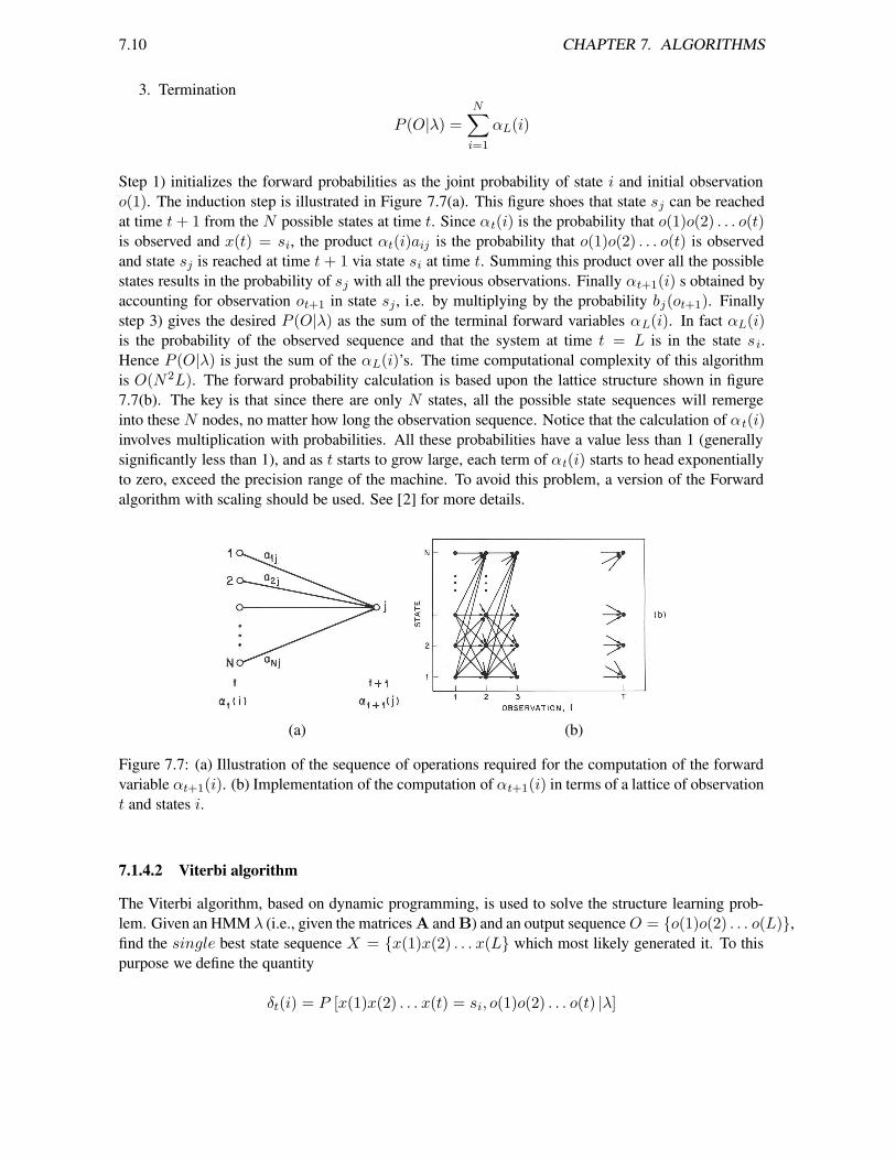
Step 1) initializes the forward probabilities as the joint probability of state i and initial observationo(1). The induction step is illustrated in Figure 7.7(a). This figure shoes that state sj can be reachedat time t+ 1 from the N possible states at time t. Since αt(i) is the probability that o(1)o(2) . . . o(t)is observed and x(t) = si, the product αt(i)aij is the probability that o(1)o(2) . . . o(t) is observedand state sj is reached at time t+ 1 via state si at time t. Summing this product over all the possiblestates results in the probability of sj with all the previous observations. Finally αt+1(i) s obtained byaccounting for observation ot+1 in state sj , i.e. by multiplying by the probability bj(ot+1). Finallystep 3) gives the desired P (O|λ) as the sum of the terminal forward variables αL(i). In fact αL(i)is the probability of the observed sequence and that the system at time t = L is in the state si.Hence P (O|λ) is just the sum of the αL(i)’s. The time computational complexity of this algorithmis O(N2L). The forward probability calculation is based upon the lattice structure shown in figure7.7(b). The key is that since there are only N states, all the possible state sequences will remergeinto these N nodes, no matter how long the observation sequence. Notice that the calculation of αt(i)involves multiplication with probabilities. All these probabilities have a value less than 1 (generallysignificantly less than 1), and as t starts to grow large, each term of αt(i) starts to head exponentiallyto zero, exceed the precision range of the machine. To avoid this problem, a version of the Forwardalgorithm with scaling should be used. See [2] for more details.

(a) (b)

Figure 7.7: (a) Illustration of the sequence of operations required for the computation of the forwardvariable αt+1(i). (b) Implementation of the computation of αt+1(i) in terms of a lattice of observationt and states i.

7.1.4.2 Viterbi algorithm

The Viterbi algorithm, based on dynamic programming, is used to solve the structure learning prob-lem. Given an HMM λ (i.e., given the matrices A and B) and an output sequenceO = {o(1)o(2) . . . o(L)},find the single best state sequence X = {x(1)x(2) . . . x(L} which most likely generated it. To thispurpose we define the quantity

δt(i) = P [x(1)x(2) . . . x(t) = si, o(1)o(2) . . . o(t) |λ]


i.e. δt(i) is the best score (highest probability) along a single path at time t, which accounts for thefirst t observations and ends in state si. By induction we have

δt+1(i) = maxi

[δt(i)aij ] bj(ot+1)

To actually retrieve the state sequence, we need to keep track of the argument which maximized theprevious expression, for each t and j using a predecessor array ψt(j). The complete procedure ofViterbi algorithm is

1. Initializationfor 1 ≤ i ≤ N

δ1(i) = π(i)bi(o1)ψ1(i) = 0

2. Inductionfor 1 ≤ t ≤ L− 1

for 1 ≤ j ≤ Nδt+1(j) = maxi [δt(i)aij ] bj(ot+1)ψt+1(j) = argmaxi [δt(i)aij ]

3. TerminationP ∗ = maxi [δT (i)]x∗(T ) = argmaxi [δT (i)]

4. Path backtrackingfor t = L− 1 downto 1

x∗(t) = ψt+1(x∗

t+1)

Notice that the structure of Viterbi algorithm is similar in implementation to forward algorithm.The major difference is the maximization over the previous states which is used in place of the sum-ming procedure in forward algorithm. Both algorithms used the lattice computational structure offigure 7.7(b) and have computational complexity N 2L. Also Viterbi algorithm presents the prob-lem of multiplicationof probabilities. One way to avoid this is to take the logarithm of the modelparameters, giving that the multiplications become additions. The induction thus becomes

log[δt+1(i)] = maxi

(log [δt(i)] + log [aij ] + log [bj(ot+1)]

Obviously will this logarithm become a problem when some model parameters has zeros present. Thisis often the case for A and π and can be avoided by adding a small number to the matrixes. See [2]for more details.

To get a better insight of how the Viterbi (and the alternative Viterbi) works, consider a modelwith N = 3 states and an observation of length L = 8. In the initialization (t = 1) is δ1(1), δ1(2) andδ1(3) found. Lets assume that δ1(2) is the maximum. Next time (t = 2) three variables will be usednamely δ2(1), δ2(2) and δ2(3). Lets assume that δ2(1) is now the maximum. In the same manner willthe following variables δ3(3), δ4(2), δ5(2), δ6(1), δ7(3) and δ8(3) be the maximum at their time, seeFig.7.8. This algorithm is an example of what is called the Breadth First Search (Viterbi employs thisessentially). In fact it follows the principle: ”Do not go to the next time instant t + 1 until the nodesat at time T are all expanded”.


Figure 7.8: Example of Viterbi search.

7.2 Commented bibliography

A good tutorial on Hidden Markov Models is [2]. Hiller and Isaacson [1] were the first to implementMarkov chains in a musical application. The application of HMM representation of musical themefor search, described in Sect. 7.1.3.1, is presented in [3].

Bibliography

[1] Lejaren A. Hiller and L. M. Isaacson. Experimental Music-Composition with an Electronic Computer. McGraw-Hill,1959.

[2] L. Rabiner. A tutorial on hidden markov models and selected applications in speech recognition. Proceeedings of theIEEE, 77(2):257–286, 1989.

[3] J. Shifrin, B. Pardo, C. Meek, and W. Birmingham. Hmm-based musical query retrieval. In Proc. ACM/IEEE JointConference on Digital Libraries, pages 295–300, 2002.

[4] Iannis Xenakis. Formalized Music. Indiana University Press, 1971.

7.13

7.14 BIBLIOGRAPHY

Contents

7 Algorithms 7.17.1 Markov Models and Hidden Markov Models . . . . . . . . . . . . . . . . . . . . . . 7.1

7.1.1 Markov Models or Markov chains . . . . . . . . . . . . . . . . . . . . . . . 7.17.1.2 Hidden Markov Models . . . . . . . . . . . . . . . . . . . . . . . . . . . . 7.37.1.3 Markov Models Applied to Music . . . . . . . . . . . . . . . . . . . . . . . 7.5

7.1.3.1 HMM models for music search: MuseArt . . . . . . . . . . . . . . 7.57.1.3.2 Markov sequence generator . . . . . . . . . . . . . . . . . . . . . 7.8

7.1.4 Algorithms . . . . . . . . . . . . . . . . . . . . . . . . . . . . . . . . . . . 7.87.1.4.1 Forward algorithm . . . . . . . . . . . . . . . . . . . . . . . . . . 7.87.1.4.2 Viterbi algorithm . . . . . . . . . . . . . . . . . . . . . . . . . . 7.10

7.2 Commented bibliography . . . . . . . . . . . . . . . . . . . . . . . . . . . . . . . . 7.12

7.15

algorithms - dei.unipd.itmusica/im06/dispense06/8_algorithms_parte1.pdf · algorithms figure 7.1:...

Documents