aliaksei maistrou - finite element method demystified
DESCRIPTION
Finite Element Method DemystifiedTRANSCRIPT

Finite Element Method Demystified
Aliaksei Maistrou

FEM definition
The finite element method (FEM) (also finite element analysis) is a numerical technique for finding approximate solutions of partial differential equations (PDE) as well as of integral equations.
The solution approach is based either on eliminating the differential equation completely (steady state problems), or rendering the PDE into an approximating system of ordinary differential equations, which are then solvedusing standard techniques such as Euler's method, Runge-Kutta, etc.

The simplest 1D example (step 1)
where f is given and u is an unknown function of x, and u'' isthe second derivative of u with respect to x
1) Convert P1 into its variational equivalent (or weak form). If u solves P1, then for any smooth function v thatsatisfies the displacement boundary conditions:
v = 0 at x = 0 and x = 1,we have

The simplest 1D example (cont’d)
where we have used the assumption that v(0) = v(1) = 0.
What we get? What can we do with it?We can choose v as any smooth function, why?
Mathematicians say we can!Then we can eliminate infinite dimensional linear problem+ minimize dimensionality of finite dimensional space

Discretization scheme (step 2)we choose the piecewise linear function vk whose value is
1 at xk and zero at every xj, j<>k, i.e.
Here we selected v as a basis with local support
The primary advantage of basis with local support is thatthe inner products
will be zero for almost all j,k

Towards numerical solution (step 3)1
0
( , ) ( ) ( )u f x x dxφ υ υ− = ∫
Assumption (that results in approximation):we can represent our functions in the form:
The weak problem will have the form:

Matrix form (step 3 cont’d)
1( ,..., )Tnf f
( )ijL L=
Advantage of basis with local support
will be zero for almost all j,k. And system matrix becomes sparse
If we denote by u and f the column vectors
and if we define
as matrices whose entries are
then we may rephrese the problem
as linear problem in matrix form:
1( ,..., )Tnu u
( )ijM M=
( , )ij i jL v vϕ= ij i jM v v= ∫

Jakob slides

Variational form (step 1)
where f is given and u is an unknown function of x, and u'' isthe second derivative of u with respect to x
1) Convert P1 into its variational equivalent (or weak form). If u solves P1, then for any smooth function v thatsatisfies the displacement boundary conditions:
v = 0 at x = 0 and x = 1,we have


Reduction to finite dim subspace Discretization (step 2)
we choose the piecewise linear function vk whose value is1 at xk and zero at every xj, j<>k, i.e.


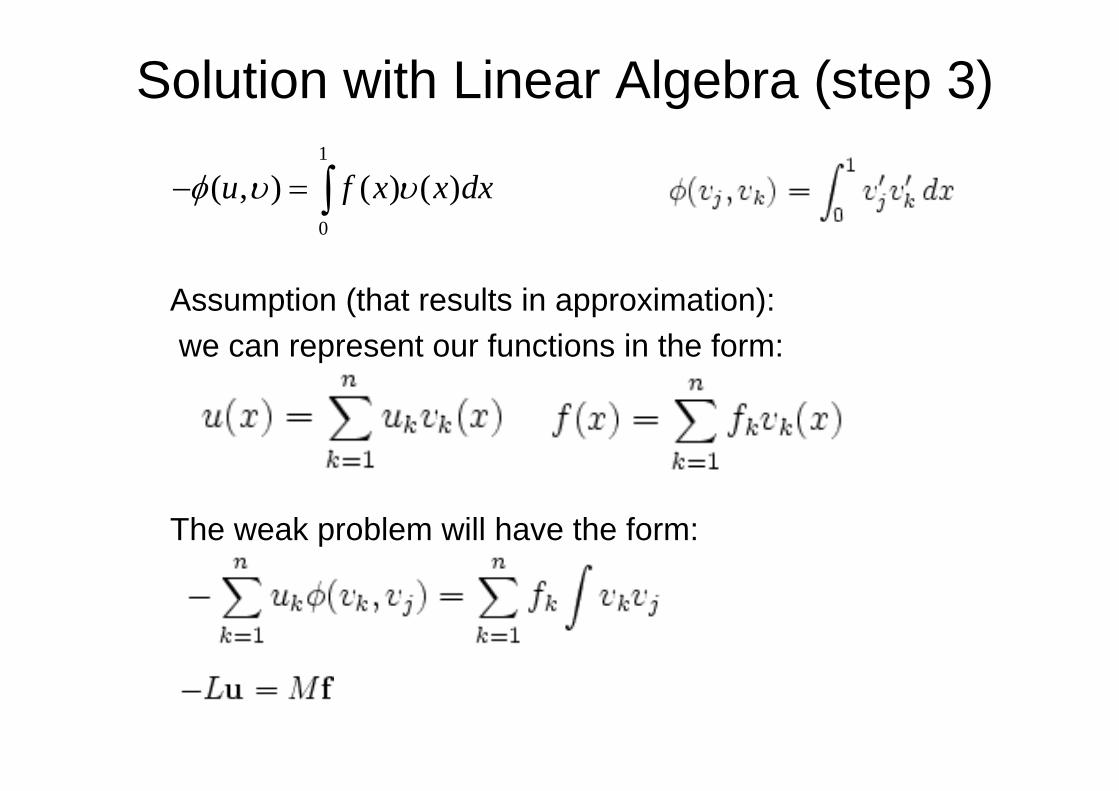
Solution with Linear Algebra (step 3)1
0
( , ) ( ) ( )u f x x dxφ υ υ− = ∫
Assumption (that results in approximation):we can represent our functions in the form:
The weak problem will have the form:


FEM: Main ingredients1) Rephrases the original PDE (boundary value
problem BVP) in its weak form. The transformation is done by hand on paper
2) The discretization. The weak form is discretized in a finite dimensional space
3) Solving a system of linear problems (LE or ODE)
Now we have concrete algorithm for a large but finite dimensionallinear problem whose solution willapproximately solve the originalBVP
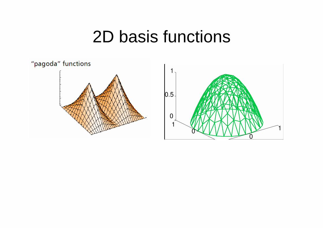
2D basis functions

1D Acoustical problems

1D Acoustical problems
Problem: find static solution (dynamical also solvable but little more complicated)
Solving using FEM
F0
1 ( , )( )
u N z tz EA z∂
=∂
zu

FEM for acoustical problem
F0
zu

FEM physical interpretation
Physical equivalent to given local support functions are spring!
F0 1 ( )u N zz EA∂
=∂
z
z
u
FF ku=

FEM physical interpretation
Energy balance for the tube:
F21 ( )u N z
z EA∂
=∂
z1 z2
F1Fc1 Fc2
2 21 1 2 2 1
1 1 ( )2 2i k u k u uΠ = + − 1 1 2 2e Fu F uΠ = − −
11
EAkl
=
22
EAkl
=
The energy of the system always tends to the minimum
i eΠ = Π +Π
1 1 2 2 2 1 11
2 2 2 1 22
0 ,
0
k u k u k u Fu
k u k u Fu
∂Π= = − + −
∂∂Π
= = − −∂
1 1
2 2
2 10
1 1/ 2u FEAu Fl
− ⎡ ⎤ ⎡ ⎤⎡ ⎤− + =⎢ ⎥ ⎢ ⎥⎢ ⎥−⎣ ⎦ ⎣ ⎦ ⎣ ⎦

FEM: principal of virtual work1 1( ) ( ) 0u uN z N z
z EA z EA∂ ∂
= ↔ − =∂ ∂
u
1
( ) ( )n
i ii
u z u zυ=
=∑
2υ1υ
1
'( ) ( ) 0n
i ii
EA u z N zυ=
− =∑
F2
z1 z2
F1
0a iW Wδ δ+ =
1 1 2 2aW F u F uδ δ δ= +
1
2
11 1 1
1 10
2 21 2 1 2 2
2 2 2 20
1( ) ' ( )
1 1((1 ) ) ' ( )
l
i
l
zW EA u u dzl l
z zEA u u u u dzl l l l
δ δ
δ δ
= − ⋅
− − + ⋅ − +
∫
∫
( ) 0uEA N zz∂
− =∂
1 1
2 2
2 10
1 1/ 2u FEAu Fl
− ⎡ ⎤ ⎡ ⎤⎡ ⎤− + =⎢ ⎥ ⎢ ⎥⎢ ⎥−⎣ ⎦ ⎣ ⎦ ⎣ ⎦
1 1 21 1
1 2 2
1 22 2
2 2
[ ( ) ]
[ ( ) ] 0
u u uW EA F ul l l
u uEA F ul l
δ δ
δ
= − + − + +
+ − + + =
1
( ) ( )n
i ii
F z f zυ=
=∑

Results?
zu
Values at 2 points! No analytical solution

FEM: Main ingredients1) Rephrases the original PDE (boundary value
problem BVP) in its weak form. The transformation is done by hand on paper
2) The discretization. The weak form is discretized in a finite dimensional space
3) Solving a system of linear problems (LE or ODE)
Now we have concrete algorithm for a large but finite dimensionallinear problem whose solution willapproximately solve the originalBVP