Contents

1 CAMEA 3

2 Description 32.1 Primary spectrometer . . . . . . . . . . . . . . . . . . . . . . . . . . . . . . . . . . . . . . . . . . 32.2 Secondary spectrometer: Prototype . . . . . . . . . . . . . . . . . . . . . . . . . . . . . . . . . . . 4

2.2.1 Detectors . . . . . . . . . . . . . . . . . . . . . . . . . . . . . . . . . . . . . . . . . . . . . 6

3 Aligning and calibrating the prototype 63.1 Aligning of the frame . . . . . . . . . . . . . . . . . . . . . . . . . . . . . . . . . . . . . . . . . . . 63.2 Mounting of the analysers . . . . . . . . . . . . . . . . . . . . . . . . . . . . . . . . . . . . . . . . 63.3 Optical alignment I . . . . . . . . . . . . . . . . . . . . . . . . . . . . . . . . . . . . . . . . . . . . 63.4 Measurement of the quality and orientations of the graphite sheets at POLDI . . . . . . . . . . . 73.5 Limits of the information from POLDI . . . . . . . . . . . . . . . . . . . . . . . . . . . . . . . . . 93.6 Measurements at Morpheus . . . . . . . . . . . . . . . . . . . . . . . . . . . . . . . . . . . . . . . 93.7 Optical alignment II. . . . . . . . . . . . . . . . . . . . . . . . . . . . . . . . . . . . . . . . . . . . 93.8 Calibration procedure . . . . . . . . . . . . . . . . . . . . . . . . . . . . . . . . . . . . . . . . . . 10

4 Measurements 104.1 Energy resolution measurements . . . . . . . . . . . . . . . . . . . . . . . . . . . . . . . . . . . . 104.2 resolution ellipsoids . . . . . . . . . . . . . . . . . . . . . . . . . . . . . . . . . . . . . . . . . . . . 114.3 Background and spurions on the prototype . . . . . . . . . . . . . . . . . . . . . . . . . . . . . . 124.4 Inelastic measurement on LiHoF4 . . . . . . . . . . . . . . . . . . . . . . . . . . . . . . . . . . . 154.5 Inelastic measurement on YMnO3 . . . . . . . . . . . . . . . . . . . . . . . . . . . . . . . . . . . 16

5 Conclusions 16

2

1 CAMEA

CAMEA (Continuous Angle Multiple Energy Analyser) is a new concept for analysing inelastically scatteredneutrons with high efficiency. It contains many (up to 10) vertically focusing analyser arrays behind eachother, analysing the scattered neutrons with a given energy by scattering them vertically. Each array analysesdifferent energies (Multiple Energy Analyser). The vertical scattering planes of analysers enable to cover largeangular range in the scattering plane (Continuous Angle). Thus CAMEA gives a fast mapping possibilities inthe three-dimensional q-ω space spanned by the horizontal q-plane and the energy transfer.

The large sample-analyser and analyser-detector distances provide clearly geometry limited energy resolution.This geometry combined with analyser crystals with relaxed mosaicity enable to use several detectors next toeach other, seeing slightly different take-off angles, thus detecting neutrons with slightly different energies. Thusthis concept has the advantages both of geometry limited resolution (high resolution) and mosaicity limitedresolution (high analysing efficiency).

CAMEA, as a secondary spectrometer can be optimally combined with a time of flight primary spectrometerresulting in an inverse geometry TOF spectrometer. ESS CAMEA is such an instrument proposed to be builtat ESS.

2 Description

The prototype of ESS CAMEA was designed to achieve a number of goals:

1. Confirm concepts: CAMEA includes a number of elements that have not been used before together.Both the overall concept of several focusing analysers behind each other simultaneously analysing differentenergies and the concept of getting several energies from one analyser. Though they work on paper someconcerns have been raised about their implementation in the real world.

2. Measure resolutions and intensities: Both simulations and analytical calculations need actual mea-surements to confirm the results. The investigated parameter space is far too big for us to measureeverything so the measurements will be used to validate the simulations.

3. Measure background: While simulations and calculations give a lot of insight into the resolutions,intensities and coverage it struggles to give realistic numbers for the background. The best way to getactual numbers is prototyping.

4. Gain experimental experience: By doing real experiments one can often learn things about how theinstrument and data analysis should work, that is not apparent in simple idealised cases such as resolutionmeasurements.

To meet these challenges the prototype was designed with a lot of flexibility so resolutions can be measured ina lot of different settings, and shielding and collimation can be installed at different places. The prototype wasplanned and built at KU and DTU and installed at the backscattering spectrometer MARS at PSI. It consist ofan Aluminum frame that contains three analyzer banks and three detector banks. Four different type of pyroliticgraphite analyser crystals have been used having 24’, 30’, 60’ and 90’ mosaic width. To maximize the flexibilityboth analysers and detectors can be moved and the Al frame allows one to mount shielding and collimatorswhere they are needed. Furthermore the chopper system of MARS was modified to adopt the rotating frequencyof the choppers to the frequency of the ESS (14Hz).

2.1 Primary spectrometer

MARS is an indirect TOF spectrometer having five choppers, with a base frequency of 50 Hz. For improvingthe resolution, the second (master) chopper can run at n*50 Hz (up to n=7). The flight path from the masterchopper to the sample is L=38.47 m. In the original concept the second chopper shapes the pulse, the firstand third choppers avoid the overlap between the pulses, and the last two, close to the sample position, are thehigher order selection choppers (the names positions, opening angles, and frequencies of the five choppers aregiven in the table 1).

3

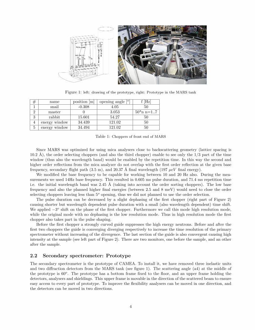
Figure 1: left: drawing of the prototype, right: Prototype in the MARS tank

# name position [m] opening angle [o] f [Hz]1 snail -0.308 4.05 502 master 0 3.053 50*n n=1..73 rabbit 15.601 54.27 504 energy window 34.439 121.02 505 energy window 34.494 121.02 50

Table 1: Choppers of front end of MARS

Since MARS was optimized for using mica analysers close to backscattering geometry (lattice spacing is10.2 A), the order selecting choppers (and also the third chopper) enable to see only the 1/3 part of the timewindow (thus also the wavelength band) would be enabled by the repetition time. In this way the second andhigher order reflections from the mica analyzer do not overlap with the first order reflection at the given basefrequency, secondary flight path (3.5 m), and 20.37 A final wavelength (197 µeV final energy).

We modified the base frequency to be capable for working between 10 and 20 Hz also. During the mea-surements we used 14Hz base frequency. This resulted in 0.605 ms pulse duration, and 71.4 ms repetition timei.e. the initial wavelength band was 2.45 A (taking into account the order sorting choppers). The low basefrequency and also the planned higher final energies (between 2.5 and 8 meV) would need to close the orderselecting choppers leaving less than 5o opening, thus we did not planned to use the order selection.

The pulse duration can be decreased by a slight dephasing of the first chopper (right part of Figure 2)causing shorter but wavelength dependent pulse duration with a small (also wavelength dependent) time shift.We applied −3o shift on the phase of the first chopper. Furthermore we call this mode high resolution mode,while the original mode with no dephasing is the low resolution mode. Thus in high resolution mode the firstchopper also takes part in the pulse shaping.

Before the first chopper a strongly curved guide suppresses the high energy neutrons. Before and after thefirst two choppers the guide is converging diverging respectively to increase the time resolution of the primaryspectrometer without increasing of the divergence. The last section of the guide is also convergent causing highintensity at the sample (see left part of Figure 2). There are two monitors, one before the sample, and an otherafter the sample.

2.2 Secondary spectrometer: Prototype

The secondary spectrometer is the prototype of CAMEA. To install it, we have removed three inelastic unitsand two diffraction detectors from the MARS tank (see figure 1). The scattering angle (a4) at the middle ofthe prototype is 60o. The prototype has a bottom frame fixed to the floor, and an upper frame holding thedetectors, analysers and shieldings. This upper frame is movable in the direction of the scattered beam to ensureeasy access to every part of prototype. To improve the flexibility analysers can be moved in one direction, andthe detectors can be moved in two directions.

4

Figure 2: left: Front end of MARS right: Effect of dephasing of the first chopper: time-flight path diagram at the firsttwo chopper. The deep blue area shows the possible trajectories of the neutrons passing through the choppers, while thelight blue line shows the trajectories of neutrons arriving to the sample in one time (and shows also the effective pulseduration at a given energy)

Analysers

The sample-analyser distance can be varied manually from 1 to 2.3 m. The analysers can be rotated slightlyaround the vertical axis by hand. Each analyzer bank has a frame rotated by motors around the horizontalaxis perpendicular to the beam direction. Each frame can hold up to 7 Si (100) wafers. Each wafer can hold15 cm2 of Pyrolytic Graphite (PG) crystals (002) - see figure 3. The wafers can be individually rotated by handto generate different focusing geometries. A number of different PG batches was bought from Panasonic (seetable 2). This system allows us to test different final neutron energies, sample analyser and analyser detector

Batch # Mosaicity (arc minutes) # of pieces Length (mm) Width (mm) Thickness (mm)1 40 15 50 10 12 40 15 50 10 13 60 10 75 10 14 90 10 75 10 15 30 15 50 10 1

Table 2: Overview of PG batches. Most of badge 1 and 2 can be combined to make a single large analyser for experimentswhere this is needed.

distances and graphite qualities.Firstly it was ensured that the wafers were uniformly oriented and the PG was approximately adjusted to

that orientation by the use of a reflected laser. Before mounting the quality and uniformity of the graphite hadto be tested and the different pieces oriented together.

Figure 3: Analyzer bank

5

2.2.1 Detectors

In each detector bank facing to one analyzer there are three position sensitive 3He detector tubes with the diam-eter of 1.26 cm (0.5”), the length of 50 cm and the position resolution of 0.5 cm. The tubes were perpendicularto the scattering plane of the analyzers, so the position along the tube can be converted into scattering angle(a4). The three tubes were next to each other, so each tube saw neutrons with a slightly different energy [1].The plane of the tubes is horizontal, but it can be tilted around the direction of the tubes by 10o to increasethe covered scattering angle range of the analysers. The energy distributions of the neutrons detected by thedifferent tubes are seen in the figure 4

Figure 4: Left: photo of detector bank, middle: Rowland geometry with three different detectors, the different colorsshow different wavelengths, right: energy distributions in the different tubes simulated by McStas

3 Aligning and calibrating the prototype

3.1 Aligning of the frame

The horizontal position, orientation and height of the frame was set by using high resolution theodolite.

3.2 Mounting of the analysers

The sizes of the crystals are 5x1 cm2 or 7.5x1 cm2 depending on their quality (see table 2). This means that asmall particle between the crystals with the size of 10 µm causes 0.06o tilting in the vertical distance if it is atthe edge of the crystal. If it is closer to the middle, then the tilting is larger. To avoid these problems, beforemounting we have carefully cleaned the whole frame, the silicon holders, the silicons, and the pyrographitecrystals using ethanol and cotton wool. We have found that even at very careful cleaning the crystals areslightly misaligned (less than 0.2o) with respect to each other. Moreover, the mounting of PG crystals on thesilicon , and also the mounting of silicons on the aluminium holder caused a bending of the silicon blades. Thedirections of the bending was the same at every mounting, thus we defined the direction of the graphite, thatthey are facing to the same direction as the fix part of the holders. In this way, the silicons remained bent closeto the holder but systematic misorientation of the PG crystals disappeared. At the beginning we did not realizethat a small force during fixation of the silicon holders cause a hole on them (where the fixing screw touchedthem). Later we have applied small cotton wool spheres as a soft spacer between the screws and the siliconholders, but often it was not useful (either they were too small, or the existing holes were in the wrong place).The holes caused large movement during fixation of the silicon holders making the precise alignment difficult.The complete change of silicon holders solved the problem and reduced the time of alignment below 15 min peranalyser. At ESS CAMEA the holders will be fixed (precisely cut from an Al mono block) so there will not besuch a problem.

3.3 Optical alignment I

After mounting of the PG crystals each blade was set to flat due to the easy checking by neutrons. For thisfirst alignment we used an optical method. We used a laser which had a double lens system. The first lens

6

produced a large elongated spot, the second one was movable and focused the light into one spot. The focusingdistance can be moved by moving the second lens. We put the laser close (30 cm) to the frame, and focused thelaser reflected by the polished silicon holder to a screen 2.5 m far from the frame. Then we shifted the frame tosee the reflected spot from each PG crystal. In this way the laser illuminated a large spot on the PG crystal,and the reflected spot on the screen showed the average surface normal of the PG. Checking each PG on theframe and also the silicon holders we got the relative orientations of the PG sheets. After this prealignmentwe checked the frames with neutrons. We found that this optical alignment is in agreement with the neutronmeasurements within the accuracy of 0.1o.

3.4 Measurement of the quality and orientations of the graphite sheets at POLDI

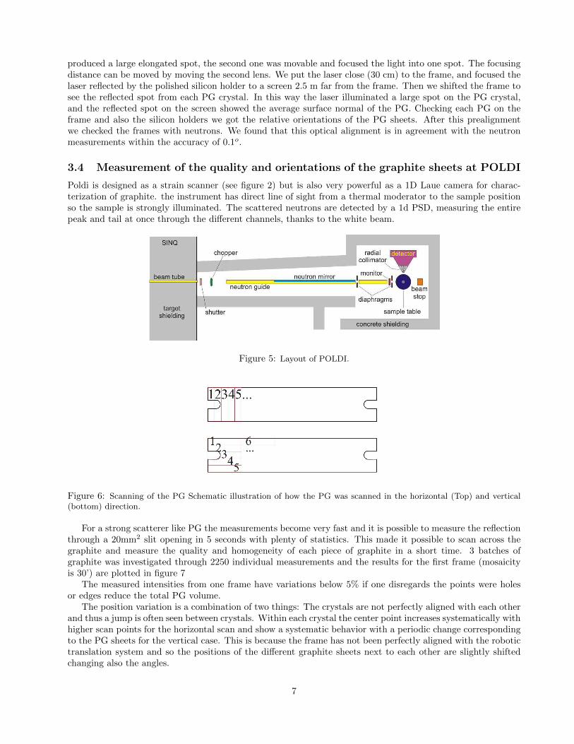
Poldi is designed as a strain scanner (see figure 2) but is also very powerful as a 1D Laue camera for charac-terization of graphite. the instrument has direct line of sight from a thermal moderator to the sample positionso the sample is strongly illuminated. The scattered neutrons are detected by a 1d PSD, measuring the entirepeak and tail at once through the different channels, thanks to the white beam.

Figure 5: Layout of POLDI.

Figure 6: Scanning of the PG Schematic illustration of how the PG was scanned in the horizontal (Top) and vertical(bottom) direction.

For a strong scatterer like PG the measurements become very fast and it is possible to measure the reflectionthrough a 20mm2 slit opening in 5 seconds with plenty of statistics. This made it possible to scan across thegraphite and measure the quality and homogeneity of each piece of graphite in a short time. 3 batches ofgraphite was investigated through 2250 individual measurements and the results for the first frame (mosaicityis 30’) are plotted in figure 7

The measured intensities from one frame have variations below 5% if one disregards the points were holesor edges reduce the total PG volume.

The position variation is a combination of two things: The crystals are not perfectly aligned with each otherand thus a jump is often seen between crystals. Within each crystal the center point increases systematically withhigher scan points for the horizontal scan and show a systematic behavior with a periodic change correspondingto the PG sheets for the vertical case. This is because the frame has not been perfectly aligned with the robotictranslation system and so the positions of the different graphite sheets next to each other are slightly shiftedchanging also the angles.

7

Figure 7: Summary of Poldi measurements The intensity(top), position(middle) and width(bottom) of the measured(0 0 2n)reflections of one batch Panasonic PG with nominal mosaicity of 40’ scanned horizontally (left) and vertically(right) The black dotted lines indicate a new crystal and the red dotted lines a new wafer. The chopper of Poldi wasstopped in open position

Both intensity and position variations are mainly due to non-perfect calibration of crystal positions andshould not raise any concerns in a study of the crystal quality, but when we look at the width of the reflectionsome effects can be seen. It is clear that some crystals are a few percent coarser than others but also that theFWHM increases close to the edges of the crystals. This is believed to be an artifact of the way the holes formounting the crystals were drilled. While it does not pose a serious risk to the prototype performance it isworth considering other ways to produce these holes in the future. For example using lasers or acids instead ofdrilling, or fix the graphite with thin aluminum straps. Two other batches with 40′ and 60′ mosaicity were alsoinvestigated. The general behavior is comparable to the first batch but reflectivity of the 60′ mosaicity is seento be about 10% lower. The number is however not completely accurate (se chp. 3.5).

8

Figure 8: Poldi measurement running the chopper at 8000 RPM.

3.5 Limits of the information from POLDI

Despite the fact that Poldi gives an excellent fast overview of the graphite performance it is not designed forsingle crystal orientation or characterisation. The angular resolution is only 5% of the typical width of themeasured PG peak, but the white thermal beam means that all of the (002), (004), (006) and (008) reflectionsare seen on top of each other. This should not influence on the position or the width of the peaks but it canmake differences in intensity bigger than what is observed only for the (002) reflection since warmer neutronshave a higher penetration depth and thus will be more influenced by a lower reflectivity than cold neutronswhere reflectivity saturation is almost reached. So while we can trust the behavior of the intensity graph weshould not trust the actual numbers. We have made a measurement with chopper running at 8000 RPM also(see Figure 8). In this case the neutrons start from pulses, and the neutrons scattered slightly smaller or larger2θ than the nominal value, thus they arrive sooner or later to the detector resulting in a tilted ellipsoid on thet-2θ map. This tilting strongly depends on the wavelength of the neutrons, thus by checking the tilting anglesof the peaks one can distinguish the different order reflections but the instrument loses the advantage of beingfast, so other instruments designed for scanning a single reflections become more advantageous.

3.6 Measurements at Morpheus

For the alignment of the different pieces of graphite the two-axis diffractometer Morpheus at PSI was used. Oneframe at a time was mounted and rocking curves (rotations of the sample around the vertical axis) recorded forthe different blades. The wavelength was λ = 5.05 A. The horizontal and vertical orientation of all crystals wasrecorded with a combination of automated and manual movement of the frame, and small pieces of aluminumfoil was inserted to coaligning the graphites. Unfortunately this also caused the Silicon wafer to bend, makingalignment an iterative process. The measured orientations were compared with laser optic measurements andit was found to agree quite well. Since optical alignment is cheaper and faster this was afterwards used forprealignment before the final alignment on Morpheus.

3.7 Optical alignment II.

Since for the different measurement geometries the corresponding Rowland geometries were also different, afterevery change in geometry we had to realign the analysers. We pushed backward the upper frame of the prototypeand, using a holder, we placed the laser at the sample position. We rotated the analyzer frame in the calculatedposition (to fulfill the Rowland condition) then we shoot one blade with the laser, and rotated the blade untilthe reflected laser beam reached the middle detector tube (see figure 9). We made it for all of the blades ofthe frame. We applied the same method for every frame starting from the back (the farthest from the sampleselecting the largest final energy). After alignment, we have removed the laser, pushed every analyzer anddetector 10 cm forward to the calculated position, and pushed the upper frame of the prototype to its originalplace.

9

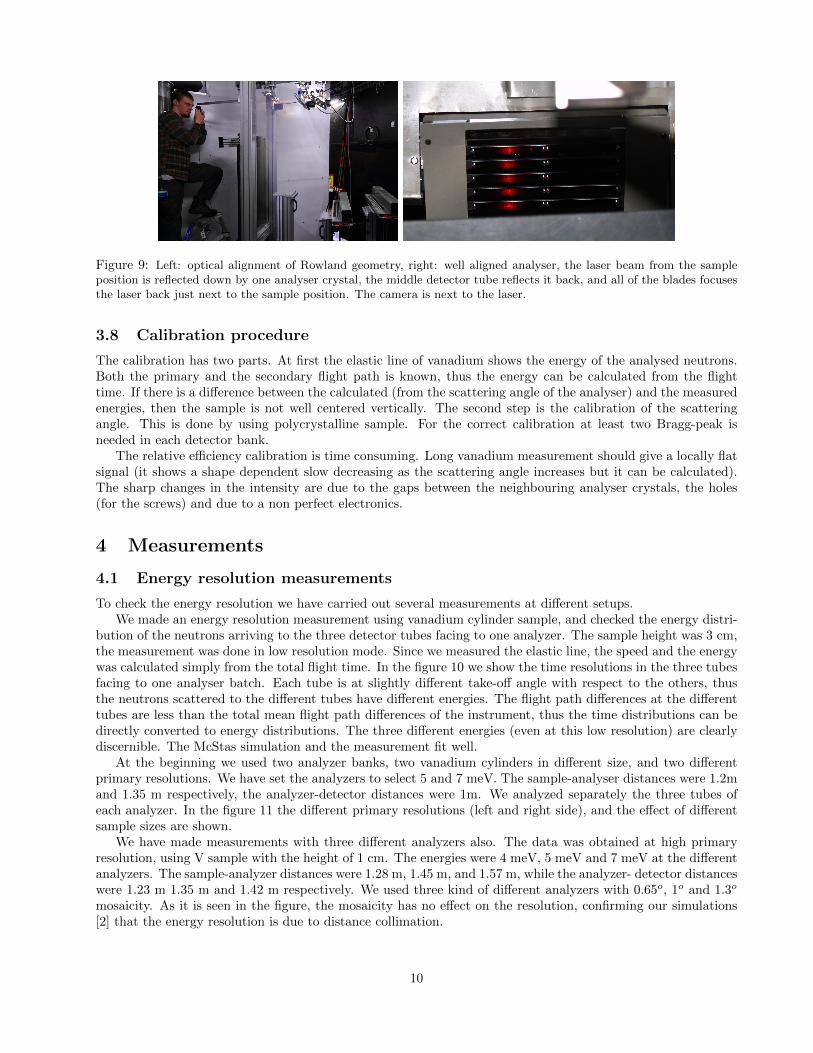
Figure 9: Left: optical alignment of Rowland geometry, right: well aligned analyser, the laser beam from the sampleposition is reflected down by one analyser crystal, the middle detector tube reflects it back, and all of the blades focusesthe laser back just next to the sample position. The camera is next to the laser.

3.8 Calibration procedure

The calibration has two parts. At first the elastic line of vanadium shows the energy of the analysed neutrons.Both the primary and the secondary flight path is known, thus the energy can be calculated from the flighttime. If there is a difference between the calculated (from the scattering angle of the analyser) and the measuredenergies, then the sample is not well centered vertically. The second step is the calibration of the scatteringangle. This is done by using polycrystalline sample. For the correct calibration at least two Bragg-peak isneeded in each detector bank.

The relative efficiency calibration is time consuming. Long vanadium measurement should give a locally flatsignal (it shows a shape dependent slow decreasing as the scattering angle increases but it can be calculated).The sharp changes in the intensity are due to the gaps between the neighbouring analyser crystals, the holes(for the screws) and due to a non perfect electronics.

4 Measurements

4.1 Energy resolution measurements

To check the energy resolution we have carried out several measurements at different setups.We made an energy resolution measurement using vanadium cylinder sample, and checked the energy distri-

bution of the neutrons arriving to the three detector tubes facing to one analyzer. The sample height was 3 cm,the measurement was done in low resolution mode. Since we measured the elastic line, the speed and the energywas calculated simply from the total flight time. In the figure 10 we show the time resolutions in the three tubesfacing to one analyser batch. Each tube is at slightly different take-off angle with respect to the others, thusthe neutrons scattered to the different tubes have different energies. The flight path differences at the differenttubes are less than the total mean flight path differences of the instrument, thus the time distributions can bedirectly converted to energy distributions. The three different energies (even at this low resolution) are clearlydiscernible. The McStas simulation and the measurement fit well.

At the beginning we used two analyzer banks, two vanadium cylinders in different size, and two differentprimary resolutions. We have set the analyzers to select 5 and 7 meV. The sample-analyser distances were 1.2mand 1.35 m respectively, the analyzer-detector distances were 1m. We analyzed separately the three tubes ofeach analyzer. In the figure 11 the different primary resolutions (left and right side), and the effect of differentsample sizes are shown.

We have made measurements with three different analyzers also. The data was obtained at high primaryresolution, using V sample with the height of 1 cm. The energies were 4 meV, 5 meV and 7 meV at the differentanalyzers. The sample-analyzer distances were 1.28 m, 1.45 m, and 1.57 m, while the analyzer- detector distanceswere 1.23 m 1.35 m and 1.42 m respectively. We used three kind of different analyzers with 0.65o, 1o and 1.3o

mosaicity. As it is seen in the figure, the mosaicity has no effect on the resolution, confirming our simulations[2] that the energy resolution is due to distance collimation.

10

Figure 10: Time distributions in the different tubes facing to one analyzer. Circles: measurement, X: McStas simulation

Figure 11: Elastic energy resolution (symbols) and the calculated energy resolution (solid lines) at different primaryresolutions (blue: high resolution, red: low resolution) and sample heights (left 3 cm, right 1 cm).

Figure 12: Elastic energy resolution (symbols) and the calculated energy resolution (solid lines) applying differentprimary resolutions and analyzers with different mosaicities (red: blue: green:).

4.2 resolution ellipsoids

We measured the resolution ellipsoids of the prototype at different setups. We used the 002 reflection of thepyrographite sample. At the given q-value the Bragg-peak can be reached only in one analyzer selecting 7meVfinal energy. In each measurement we made an omega (a3) scan around the Bragg position of the sample. Onemeasurement of the scan gave three parabolic surfaces close to each other in the q-w space (taking into accountthat the three tubes looking to the analyser collect neutrons with slightly different final energies). We chosethe qx-direction parallel to the corresponding reciprocal lattice vector, qy is perpendicular to it. We summedup the data in the three dimensional q − ω space, and in the figures below we show the data projected to theplanes (E=0, qx=0 and qy=0).

The figures 13 - 14 shows the measured and calculated ([2]) resolution ellipsoids. In the Figure 13 - 17 theresolution ellipsoids measured under different conditions are seen. Each figure is normalized to its maximumintensity, so the color bars are the same for each figure. In the figure 13 and 14 the difference between themeasurements made using a sample with high and low mosaicity (0.5 and 1.5 degree) is clearly seen. (Thefinite mosaicity of the sample causes a smearing in the qy direction). In the figures 15 and 16 the effect ofthe mosaicity of the analyser (0.6 and 1.3 degree respectively) is seen. The tangential resolution is increasingwith the mosaicity, while the energy resolution does not change. The last (17) figure the worse q-resolution is

11

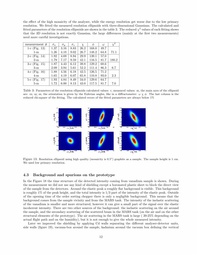
the effect of the high mosaicity of the analyzer, while the energy resolution get worse due to the low primaryresolution. We fitted the measured resolution ellipsoids with three-dimensional Gaussians. The calculated andfitted parameters of the resolution ellipsoids are shown in the table 3. The reduced χ2 values of each fitting showsthat the 3D resolution is not exactly Gaussian, the large differences (mainly at the first two measurements)need more careful investigations.

measurement # σx σy σz χ φ ω χ2

1-c (Fig. 13) 1.37 3.16 8.83 26.2 168.0 49.71-m 1.26 4.18 9.02 26.7 148.2 64.8 71.1

2-c (Fig. 14) 1.92 4.69 8.94 29.9 139.1 57.02-m 1.79 7.17 9.59 42.1 116.5 81.7 180.2

3-c (Fig. 15) 1.87 4.43 6.12 39.8 129.2 68.63-m 2.09 3.94 5.61 52.2 111.4 86.3 6.7

4-c (Fig. 16) 1.88 4.56 6.18 42.5 126.5 71.24-m 1.65 4.19 6.07 65.8 110.8 93.0 2.3

5-c (Fig. 17) 1.93 4.84 8.49 34.0 129.6 64.75-m 1.72 6.00 8.13 43.0 117.5 81.7 7.0

Table 3: Parameters of the resolution ellipsoids calculated values: c, measured values: m, the main axes of the ellipsoidare: sx, sy, sz, the orientation is given by the Eulerian angles, like in a diffractometer: ω χ φ. The last column is thereduced chi-square of the fitting. The calculated errors of the fitted parameters are always below 1%

Figure 13: Resolution ellipsoid using high quality (mosaicity is 0.5o) graphite as a sample. The sample height is 1 cm.We used low primary resolution.

4.3 Background and spurions on the prototype

In the Figure 18 the time structure of the detected intensity coming from vanadium sample is shown. Duringthe measurement we did not use any kind of shielding except a boronated plastic sheet to block the direct viewof the sample from the detectors. Around the elastic peak a roughly flat background is visible. This backgroundis roughly 1% of the peak height, and the total intensity is 1/3 part of the intensity of the elastic peak. Outsideof the opening time of the order sorting chopper there is only a negligible background. This means that thebackground comes from the sample vicinity and from the MARS tank. The intensity of the inelastic scatteringof the vanadium is smaller and more structured, however it can give a small part of the signal over the elasticincoherent intensity. There are two other sources of the background: the inelastic scattering on the air aroundthe sample, and the secondary scattering of the scattered beam in the MARS tank (on the air and on the otherstructural elements of the prototype). The air scattering in the MARS tank is large ( 20-25% depending on theactual flight path and on the humidity), but it is not enough to give the whole measured intensity.

Later we improved the shielding by applying Cd walls separating the different analyser-detector units,side walls (figure 19), vacuum-box around the sample, kadmium around the vacuum box defining the vertical

12

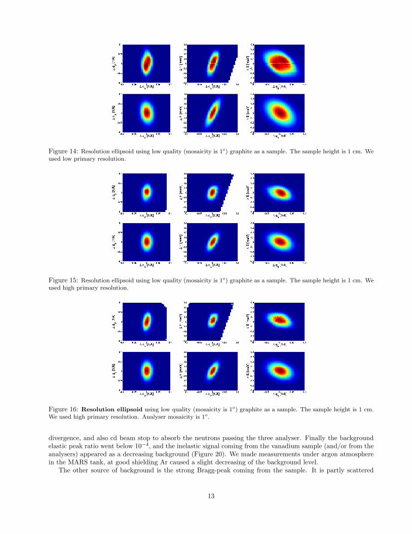
Figure 14: Resolution ellipsoid using low quality (mosaicity is 1o) graphite as a sample. The sample height is 1 cm. Weused low primary resolution.

Figure 15: Resolution ellipsoid using low quality (mosaicity is 1o) graphite as a sample. The sample height is 1 cm. Weused high primary resolution.

Figure 16: Resolution ellipsoid using low quality (mosaicity is 1o) graphite as a sample. The sample height is 1 cm.We used high primary resolution. Analyser mosaicity is 1o.

divergence, and also cd beam stop to absorb the neutrons passing the three analyser. Finally the backgroundelastic peak ratio went below 10−4, and the inelastic signal coming from the vanadium sample (and/or from theanalysers) appeared as a decreasing background (Figure 20). We made measurements under argon atmospherein the MARS tank, at good shielding Ar caused a slight decreasing of the background level.

The other source of background is the strong Bragg-peak coming from the sample. It is partly scattered

13

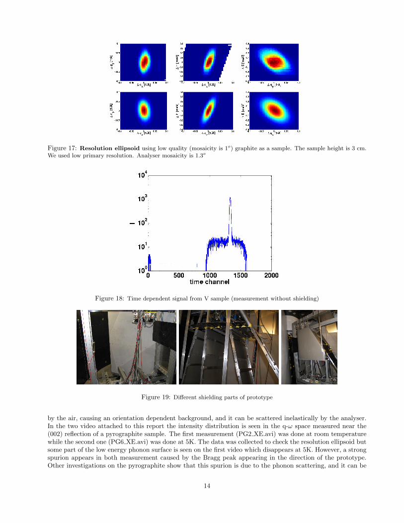
Figure 17: Resolution ellipsoid using low quality (mosaicity is 1o) graphite as a sample. The sample height is 3 cm.We used low primary resolution. Analyser mosaicity is 1.3o

Figure 18: Time dependent signal from V sample (measurement without shielding)

Figure 19: Different shielding parts of prototype

by the air, causing an orientation dependent background, and it can be scattered inelastically by the analyser.In the two video attached to this report the intensity distribution is seen in the q-ω space measured near the(002) reflection of a pyrographite sample. The first measurement (PG2 XE.avi) was done at room temperaturewhile the second one (PG6 XE.avi) was done at 5K. The data was collected to check the resolution ellipsoid butsome part of the low energy phonon surface is seen on the first video which disappears at 5K. However, a strongspurion appears in both measurement caused by the Bragg peak appearing in the direction of the prototype.Other investigations on the pyrographite show that this spurion is due to the phonon scattering, and it can be

14

Figure 20: Time dependent signal from room temperature and cooled V sample, and the effect of the Ar atmosphere.On the right side the electronic background is shown.

reduced by cooling the crystals [3].

4.4 Inelastic measurement on LiHoF4

We have made an inelastic measurement on LiHoF4 sample at four different temperatures. LiHoF4 has strongcrystal field excitations at low temperature. The sample consist many plate-like large single crystal stackedtogether. The data obtained at 14Hz base frequency, with low primary resolution within ca 3h at each tempera-ture. In the left part of Figure 21 the measurements at four different temperatures are seen. We made the samemeasurement at Focus (direct TOF instrument). After correcting with difference of the detected angular area,we get similar intensity but much better resolution (right part of Figure 21. To compare the two measurements,the only data treatment was the summing up on energy channels, normalizing for the time, and applying thecorrection factor for the detected angular area. The green line shows the summed data on the 9 tub es, whilethe red line shows the data normalized to the number of tubes also. With the angular coverage of the ESSCAMEA at the prototype we could get roughly three times more detected intensity than at FOCUS.

Figure 21: Inelastic measurement on LiHoF4 sample. Left: measurement in the prototype at 4K (blue), 25K (green),25K ( red), and 70K (magenta). The base line of each data is shifted for the sake of visibility. Right: Comparison ofmeasurements at the prototype and at Focus. The counts summed in energy bin and normalized to monitor.

15

4.5 Inelastic measurement on YMnO3

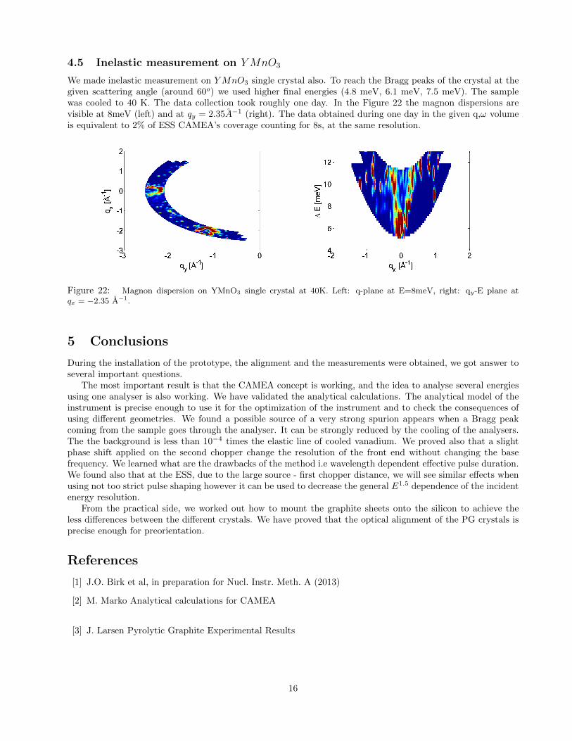
We made inelastic measurement on YMnO3 single crystal also. To reach the Bragg peaks of the crystal at thegiven scattering angle (around 60o) we used higher final energies (4.8 meV, 6.1 meV, 7.5 meV). The samplewas cooled to 40 K. The data collection took roughly one day. In the Figure 22 the magnon dispersions arevisible at 8meV (left) and at qy = 2.35A−1 (right). The data obtained during one day in the given q,ω volumeis equivalent to 2% of ESS CAMEA’s coverage counting for 8s, at the same resolution.

Figure 22: Magnon dispersion on YMnO3 single crystal at 40K. Left: q-plane at E=8meV, right: qy-E plane atqx = −2.35 A−1.

5 Conclusions

During the installation of the prototype, the alignment and the measurements were obtained, we got answer toseveral important questions.

The most important result is that the CAMEA concept is working, and the idea to analyse several energiesusing one analyser is also working. We have validated the analytical calculations. The analytical model of theinstrument is precise enough to use it for the optimization of the instrument and to check the consequences ofusing different geometries. We found a possible source of a very strong spurion appears when a Bragg peakcoming from the sample goes through the analyser. It can be strongly reduced by the cooling of the analysers.The the background is less than 10−4 times the elastic line of cooled vanadium. We proved also that a slightphase shift applied on the second chopper change the resolution of the front end without changing the basefrequency. We learned what are the drawbacks of the method i.e wavelength dependent effective pulse duration.We found also that at the ESS, due to the large source - first chopper distance, we will see similar effects whenusing not too strict pulse shaping however it can be used to decrease the general E1.5 dependence of the incidentenergy resolution.

From the practical side, we worked out how to mount the graphite sheets onto the silicon to achieve theless differences between the different crystals. We have proved that the optical alignment of the PG crystals isprecise enough for preorientation.

References

[1] J.O. Birk et al, in preparation for Nucl. Instr. Meth. A (2013)

[2] M. Marko Analytical calculations for CAMEA

[3] J. Larsen Pyrolytic Graphite Experimental Results

16