A L I S O N BO W L I N G

THE GENERAL LINEAR MODEL

THE GENERAL LINEAR MODEL

• the observed score for the ith observation• .. the scores on the predictor variables for the ith

observation• intercept (value of Y when all the predictors are

0)• …. coefficients – rate of change in Y for each one

unit change in X• the residual

ALTERNATIVE EXPRESSION OF THE MODEL

• is the predicted (or expected value of Y)

PREDICTORS (IVS)

• Continuous (covariates)• E.g. age, weight, time

• Dichotomous• E.g. male vs female, employed vs

unemployed, control vs experiment, low dose vs placebo, high dose vs placebo

• Dichotomous variables are usually Dummy coded.• Reference group = 0 e.g. male• Comparison group = 1 e.g. female

GLM APPROACH TO ANOVA

• ANOVA is one instance of the General Linear Model• Field Viagra.sav

Group Low High

Placebo 0 0

Low Dose Viagra

1 0

High Dose Viagra

0 1

REGRESSION ANALYSIS

INTERPRETING THE COEFFICIENTS

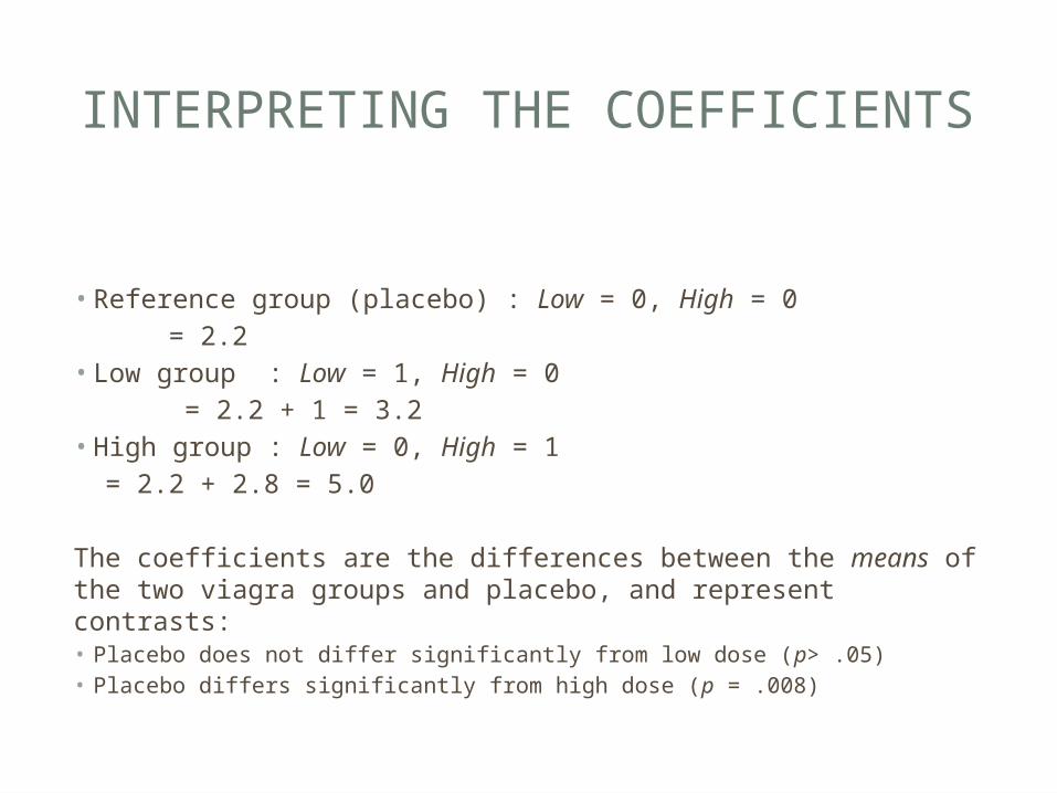
• Reference group (placebo) : Low = 0, High = 0 = 2.2• Low group : Low = 1, High = 0 = 2.2 + 1 = 3.2• High group : Low = 0, High = 1 = 2.2 + 2.8 = 5.0

The coefficients are the differences between the means of the two viagra groups and placebo, and represent contrasts:• Placebo does not differ significantly from low dose (p> .05)• Placebo differs significantly from high dose (p = .008)

GLM

ANOVA OUTPUT

• The GLM Univariate procedure runs a General Linear Model, with the IV automatically dummy coded so that the group with the highest code is treated as the reference category.• The intercept is the mean of the High dose group• The dose = 1 (placebo) coefficient is the

difference between the mean of the high dose and placebo group, and is significant (p = .008)• The dose = 2 (low) coefficient is the difference

between the mean of the high and low doses (NS).

WHY IS THIS IMPORTANT?

• Enables us to build sophisticated models including both continuous and categorical predictors• Enhances understanding covariance

• Necessary to build regression models in which the assumptions are violated.

BRIEF REVISION OF MULTIPLE REGRESSION

• Multiple regression with two or more continuous predictors• When the predictors are correlated, the coefficients

represent the effect each predictor in the model, taking into account the other predictors.• i.e. the effect of a predictor after the correlation(s) with the

other predictors are partialled out.

• Field (2013) album sales.sav• DV: Album sales• Predictors: Advertising budget, No of plays on radio,

Attractiveness of the band.

BIVARIATE SCATTERPLOTS

CORRELATIONS

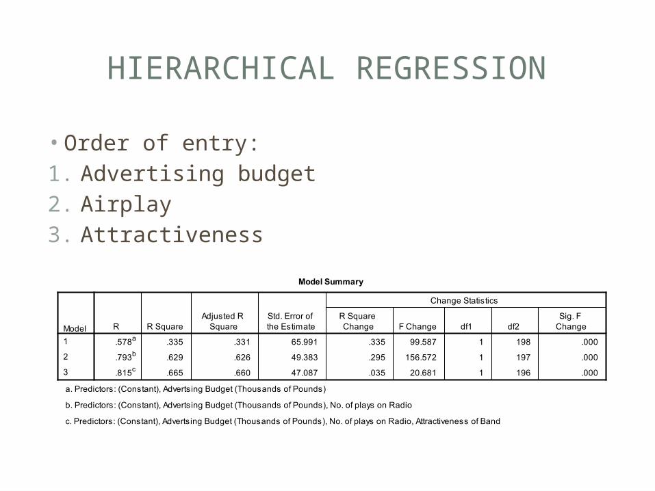
HIERARCHICAL REGRESSION

• Order of entry: 1. Advertising budget2. Airplay3. Attractiveness

COEFFICIENTS

MODEL

• Coefficients are the amount of change in Y, for one unit change in X• Magnitude depends on the magnitude of the Xs

COGNITION AND ANTI-SACCADE DATA(PETER LINDSAY)

• DV: Percentage of anti-saccade errors• Predictors: Visuospatial/constructional, Delayed

memory.• Predictors are correlated

HIERARCHICAL REGRESSION

Delayed memory does not improve the prediction of errors, after controlling for visuospatial

CHECKING RESIDUALS FOR NORMALITY

• Residuals are skewed – DV is a proportion, and therefore likely to violate assumptions.

ANALYSIS OF COVARIANCE

• One continuous and one categorical predictor• Field (2013) ViagraCovariate.sav;

ViagracovariateDummy.sav

• DV Libido• IV Viagra dose• Covariate: Partner’s libido• Model:

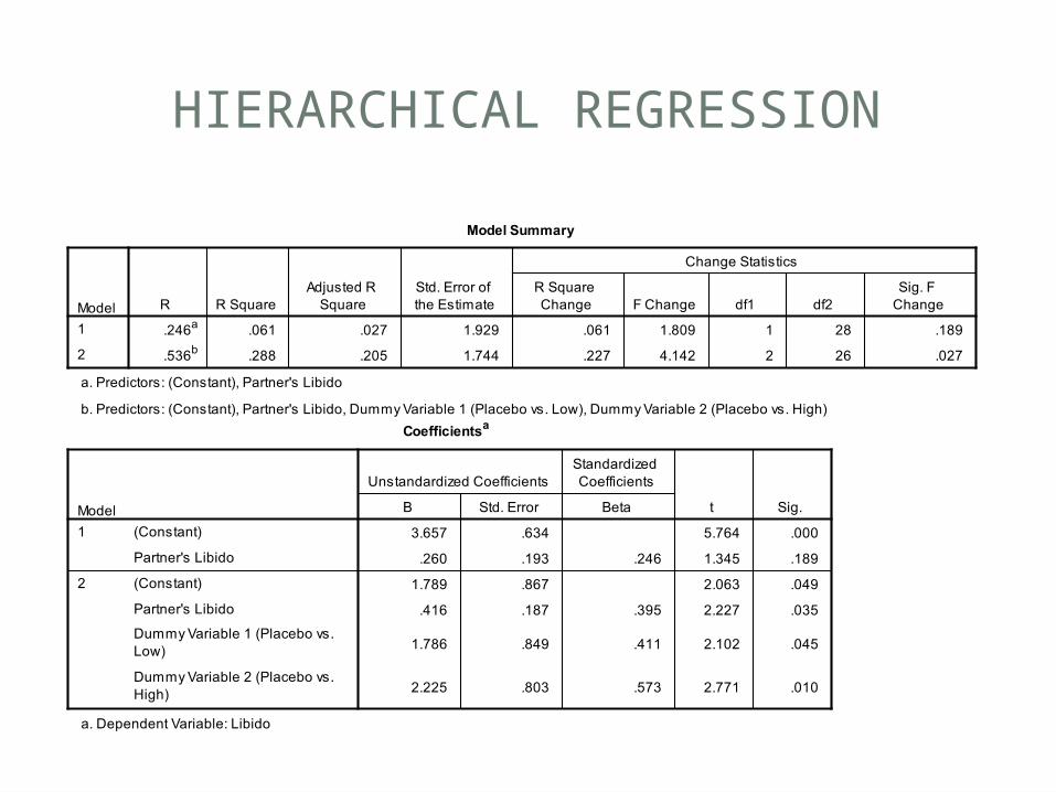
HIERARCHICAL REGRESSION

ANCOVA

The effect of Dose is the effect of Viagra, after controlling for the covariate.

ASSUMPTIONS AND DATA ISSUES

• Main assumption of the model• Residuals (not DV) are normally distributed

• Data issues (relate to the data or mathematics)• Mulitcollinearity• Outliers• Non-linearity• Etc.

• If the DV is continuous, unbounded and measured on an interval or ratio scale, the assumptions are most likely met.

• Not otherwise.

WHAT TO DO WHEN THE ASSUMPTIONS ARE VIOLATED

• In Psychology, our DV is sometimes a proportion or a count.• In this case, the normality assumption is often

violated.• When assumptions are broken, use• Generalised Linear Models• These apply a link function (f) to the DV to create a linear

model.• f (Y) =

COMMON LINK FUNCTIONS

• Logit (log odds) for proportions• Logistic regression

• Poisson (log) for count data• Negative binomial for count data.

GENERALISED LINEAR MODELS

• Parameter estimation• Linear models use Ordinary Least Squares (OLS) to

estimate parameters.• This is done by minimising the sum of the squared residuals• R2 is the measure of goodness-of-fit of the model

• Generalised linear models use Maximum Likelihood as the method of estimation.• Negative Log Likelihood (-2LL) is one of several measures of

goodness of fit.

MORE SOPHISTICATED MODELS

• Mixed models• These may be used as an alternative method of analysing

repeated measures data.• Includes random effects in the model• Models the variance of the intercept and/or the slope

• Generalised Linear mixed models• More sophisticated still• Applies mixed model methodology to Generalised linear

models.

• All of these use Maximum Likelihood.