Algorithmic Representation of Visual

Information

Daby M. Sow

Submitted in partial ful�llment of the

requirements for the degree of

Doctor of Philosophy

in the Graduate School of Arts and Sciences

Columbia University

2000

c 2000

Daby M. Sow

All Rights Reserved

ABSTRACT

Algorithmic Representation of Visual Information

Daby M. Sow

This thesis presents new perspectives to media representation and addresses fun-

damental source coding problems outside the umbrella of traditional information

theory, namely, the representation of �nite individual objects with a �nite amount

of computational resources. We start by proposing a new theory, Complexity Dis-

tortion Theory, which uses programmatic descriptions to provide a mathematical

framework where these problems can be addressed. The key component of this

theory is the substitution of the decoder in Shannon's communication system by a

computer. The mathematical framework for examining issues of e�ciency is then

Kolmogorov Complexity Theory. Complexity Distortion Theory extends this frame-

work to include distortion by de�ning the complexity distortion function, the equiv-

alent to the rate distortion function in this algorithmic setting. We show that this

information measure predicts asymptotically the same results as the classical proba-

bilistic information measures, for stationary and ergodic sources. These equivalences

highlight the duality between Shannon and Kolmogorov's information measures.

The former de�nes information as a set notion that requires the estimation of rel-

ative frequencies to predict asymptotic results whereas the latter is a deterministic

concept de�ning randomness for individual objects. It allows us to formalize the

universal coding problem for �nite individual objects. This then closes the circle of

media representation techniques, from probabilistic to deterministic approaches. It

also opens new horizons outside the scope of classical source coding that we explore

in the second part of this thesis. In contrast with the classical approach, computa-

tional resource bounds can be introduced naturally at the decoding end. This way,

we add a new dimension to source coding theory, extending the rate distortion curve

to a complexity distortion surface representing the tradeo� between rate, distortion

and computational complexity. Understanding this complex tradeo� is key for the

design of e�cient decoders with e�cient computational resource management capa-

bilities. In the last part of this thesis, we approximate this surface in a constructive

fashion yielding a new class of algorithms for the universal coding of �nite objects

under distortion and computational constraints. An extensive analysis of the con-

vergence properties of these algorithms is presented together with their application

to still image data.

Contents

1 Introduction 1

1.1. Introduction : : : : : : : : : : : : : : : : : : : : : : : : : : : : : : : : 1

1.2. Thesis Contributions : : : : : : : : : : : : : : : : : : : : : : : : : : : 9

1.2.1 Complexity Distortion Theory : : : : : : : : : : : : : : : : : : 9

1.2.2 Resource Bounds in Media Representation : : : : : : : : : : : 10

1.2.3 Universal Coding of Finite Objects : : : : : : : : : : : : : : : 12

1.3. Outline of Thesis : : : : : : : : : : : : : : : : : : : : : : : : : : : : : 13

2 Classical Information and Rate Distortion Theories 15

2.1. Introduction : : : : : : : : : : : : : : : : : : : : : : : : : : : : : : : : 15

2.2. Information Sources and Notations : : : : : : : : : : : : : : : : : : : 19

2.3. Information Measures : : : : : : : : : : : : : : : : : : : : : : : : : : : 24

2.3.1 Lossless Measures : : : : : : : : : : : : : : : : : : : : : : : : : 24

2.3.2 Lossy Measures : : : : : : : : : : : : : : : : : : : : : : : : : : 27

2.4. Source Coding Theorem and Universal Coding : : : : : : : : : : : : : 32

2.5. Conclusion : : : : : : : : : : : : : : : : : : : : : : : : : : : : : : : : : 38

3 Complexity Distortion Theory 40

3.1. Introduction : : : : : : : : : : : : : : : : : : : : : : : : : : : : : : : : 40

3.2. Universal Turing Machines : : : : : : : : : : : : : : : : : : : : : : : : 43

i

3.3. Kolmogorov Complexity : : : : : : : : : : : : : : : : : : : : : : : : : 46

3.3.1 Individual Information Measure : : : : : : : : : : : : : : : : : 48

3.3.2 Randomness Tests : : : : : : : : : : : : : : : : : : : : : : : : 53

3.4. Equivalence with Information Theory : : : : : : : : : : : : : : : : : : 55

3.4.1 Fundamental Theorem : : : : : : : : : : : : : : : : : : : : : : 55

3.4.2 Proof of Fundamental Theorem : : : : : : : : : : : : : : : : : 58

3.5. Complexity Distortion Function : : : : : : : : : : : : : : : : : : : : : 61

3.6. Equivalence with Rate Distortion Theory : : : : : : : : : : : : : : : : 62

3.6.1 Extended Fundamental Theorem : : : : : : : : : : : : : : : : 62

3.6.2 Proof of Extended Fundamental Theorem : : : : : : : : : : : 64

3.6.3 Some Remarks : : : : : : : : : : : : : : : : : : : : : : : : : : 72

3.7. Conclusion : : : : : : : : : : : : : : : : : : : : : : : : : : : : : : : : : 73

4 Resource Bounds in Media Representation 75

4.1. Introduction : : : : : : : : : : : : : : : : : : : : : : : : : : : : : : : : 75

4.2. Resource Bounded Complexity Distortion Function : : : : : : : : : : 78

4.3. Universal Coding of Finite Objects with Distortion and Computa-

tional Constraints : : : : : : : : : : : : : : : : : : : : : : : : : : : : : 88

4.3.1 Universal Coding Revisited : : : : : : : : : : : : : : : : : : : 90

4.3.2 The Decoder : : : : : : : : : : : : : : : : : : : : : : : : : : : 93

4.3.3 The Encoder : : : : : : : : : : : : : : : : : : : : : : : : : : : 94

4.4. Convergence Analysis of Genetic Programming : : : : : : : : : : : : : 97

4.4.1 Convergence : : : : : : : : : : : : : : : : : : : : : : : : : : : : 101

4.4.2 Speed of Convergence : : : : : : : : : : : : : : : : : : : : : : : 103

4.5. Algorithmic Representation of Images : : : : : : : : : : : : : : : : : : 109

4.5.1 The Decoder : : : : : : : : : : : : : : : : : : : : : : : : : : : 109

4.5.2 The Encoder : : : : : : : : : : : : : : : : : : : : : : : : : : : 111

ii

4.6. Conclusion : : : : : : : : : : : : : : : : : : : : : : : : : : : : : : : : : 116

5 Conclusion and future directions 119

5.1. Conclusion : : : : : : : : : : : : : : : : : : : : : : : : : : : : : : : : : 119

5.2. Future directions : : : : : : : : : : : : : : : : : : : : : : : : : : : : : 121

5.2.1 Channel Capacity versus System Capacity : : : : : : : : : : : 121

5.2.2 Language Design : : : : : : : : : : : : : : : : : : : : : : : : : 123

References 125

Appendix 133

A. Recursive Functions : : : : : : : : : : : : : : : : : : : : : : : : : : : : 133

B. Randomness Tests : : : : : : : : : : : : : : : : : : : : : : : : : : : : 134

C. Markov Types : : : : : : : : : : : : : : : : : : : : : : : : : : : : : : : 137

iii

List of Figures

2-1 Shannon's communication system. The signals transmitted on the

channels represent codewords. They are typically indices to repro-

duction sequences on which redundancy bits have been added for

error correction. : : : : : : : : : : : : : : : : : : : : : : : : : : : : : : 16

2-2 The separation between source and channel coding at the transmitter.

In this thesis, we focus on the source coding operations. : : : : : : : : 17

2-3 The shift operator on two-way in�nite sequences : : : : : : : : : : : : 21

2-4 A stationary information source. Initially, the initial mode choice

module selects one of the stationary sources and the source stays in

this mode for the rest of its operation. Hence from any long observa-

tion of the source, we can estimate the distribution of one particular

stationary source. This source would be ergodic if the initial mode

choice almost always select the same stationary source i; 1 � i � m. : 22

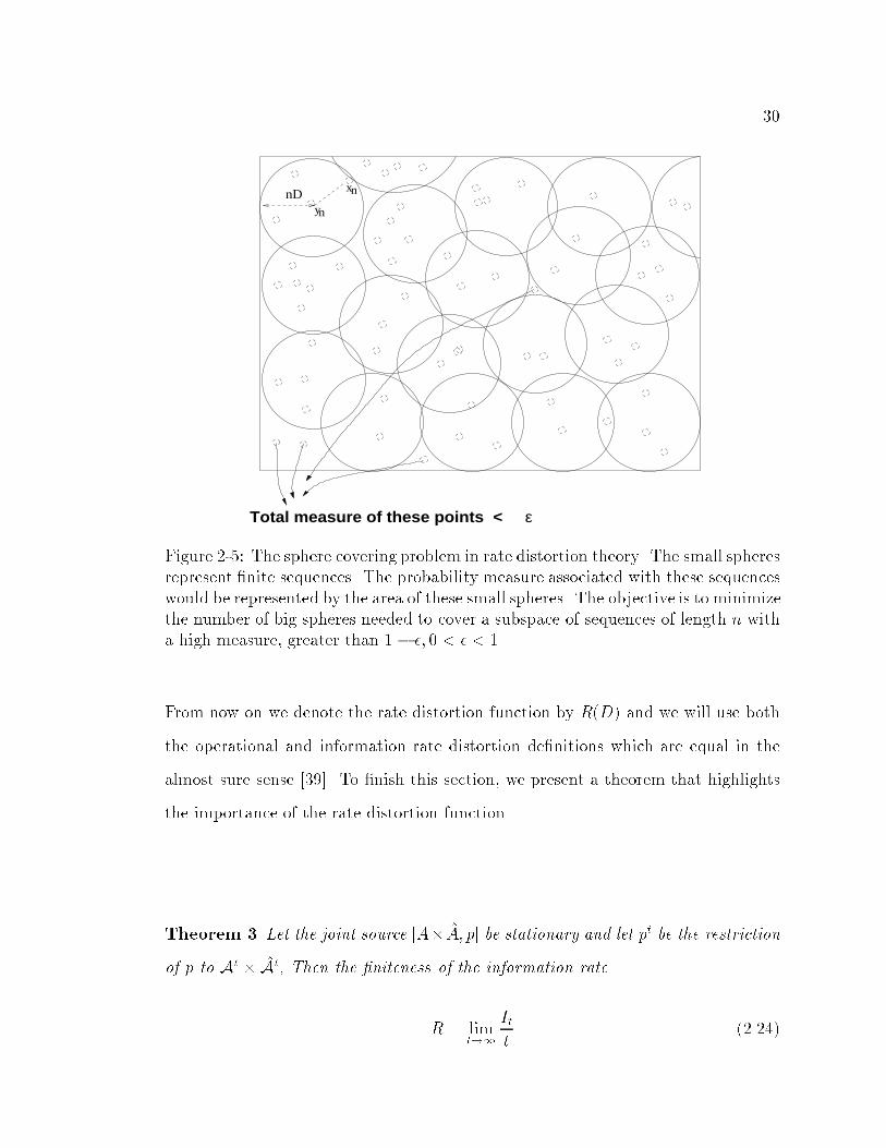
2-5 The sphere covering problem in rate distortion theory. The small

spheres represent �nite sequences. The probability measure associ-

ated with these sequences would be represented by the area of these

small spheres. The objective is to minimize the number of big spheres

needed to cover a subspace of sequences of length n with a high mea-

sure, greater than 1� �; 0 < � < 1. : : : : : : : : : : : : : : : : : : : : 30

2-6 Universal Coding System type I. : : : : : : : : : : : : : : : : : : : : : 35

iv

2-7 Universal Coding System type II. : : : : : : : : : : : : : : : : : : : : 36

2-8 Universal Coding System type III. : : : : : : : : : : : : : : : : : : : : 36

2-9 Universal coding and the separation principle between model and data. 39

3-1 Finite Automaton: The top �gure shows the transition diagram of

a �nite automaton. Assuming that the initial and �nal state are

both q0, this automaton will recognize all sequences in which both

the number of 0's and the number of 1's is even. The example shown

in the bottom will leave the automaton in state q3 at the end of the

computation. : : : : : : : : : : : : : : : : : : : : : : : : : : : : : : : 44

3-2 A Turing machine with one work or memory tape. : : : : : : : : : : : 45

3-3 The programmable communication system. Notice that two-part

codes representing algorithms and data are sent through the chan-

nel. We call this communication system Kolmogorov's communica-

tion system. : : : : : : : : : : : : : : : : : : : : : : : : : : : : : : : : 47

3-4 Duality between Shannon's entropy and Kolmogorov complexity. : : : 54

3-5 The circle of media representation theories (the bottom-right box as

well as its associated arrows, establishing its relationship with other

theories, are introduced in this thesis). : : : : : : : : : : : : : : : : : 64

4-1 Rate-Distortion-Complexity tradeo�. : : : : : : : : : : : : : : : : : : 81

4-2 Algorithmically universal coding system. This system generalizes the

�rst three universal coding systems presented in chapter 2, section 2.4. 92

4-3 The transition matrix for the elitist strategy. : : : : : : : : : : : : : : 106

4-4 Hybrid Image Encoder. : : : : : : : : : : : : : : : : : : : : : : : : : : 112

4-5 This �gure shows how the memory indexing is done, relatively to the

position of the current block. : : : : : : : : : : : : : : : : : : : : : : : 113

v

4-6 Programmatic representation of lenna 512x512, psnr = 29.72 dB at

1.17 bpp: (a) original, (b) gp output. In this run the language uses

4x4 blocks. Note the large errors introduced in the top of the picture

because of the inability of the language to represent these blocks when

the memory of the system is empty. : : : : : : : : : : : : : : : : : : : 114

4-7 This �gure compares 8x8 blocks with a signi�cant amount of edges

(according to a Sobel edge detector) with blocks that cannot be rep-

resented accurately by the GP module. Edge blocks and GP blocks

with large MSE are in white: (a) edge blocks, (b) GP blocks with

large error. Note the similarities between this two pictures showing

that the language did not manage to represent accurately most of the

edge blocks. : : : : : : : : : : : : : : : : : : : : : : : : : : : : : : : 115

4-8 Programmatic representation of lenna 512x512 with the learning unit,

psnr = 32.97 dB at 0.9 bpp: (a) original, (b) gp output. In this run

the language uses 8x8 blocks. The learning unit introduced 1381

DCT blocks (out of 4096), mainly at the strong edges of the image. : 116

4-9 Programmatic representation of house 256x256 with the learning unit,

psnr = 35.75 dB at 0.9 bpp: (a) original, (b) gp output. In this run

the language uses 8x8 blocks. The learning unit introduced 425 DCT

blocks (out of 1024), mainly at the strong edges of the image : : : : : 117

4-10 Programmatic representation of peppers 256x256 with the learning

unit, psnr = 34.02 dB at 1.9 bpp: (a) original, (b) gp output. In this

run the language uses 8x8 blocks. The learning unit introduced 643

DCT blocks (out of 1024), mainly at the strong edges of the image : : 117

5-1 Channel and system capacities. : : : : : : : : : : : : : : : : : : : : : 122

5-2 General system channel. : : : : : : : : : : : : : : : : : : : : : : : : : 123

vi

List of Tables

4.1 Functions used to represent gray level image data. : : : : : : : : : : 110

4.2 Terminals used to represent gray level image data. : : : : : : : : : : 111

vii

List of Abbreviations

AEP Asymptotic Equipartition PropertyCDF Complexity Distortion FunctionCDT Complexity Distortion TheoryDCT Discrete Cosine TransformFA Finite AutomataFSM Finite State MachineGA Genetic AlgorithmGP Genetic ProgrammingHVS Human Visual SystemIT Information TheoryJPEG Joint Photography Experts GroupKLT Karhunen Loeve TransformMAP Maximum a posterioriMDL Minimum Description LengthML Maximum LikelihoodMPEG Moving Picture Experts GroupMSE Mean Square ErrorPSNR Peak Signal to Noise RatioRDF Rate Distortion FunctionRDT Rate Distortion TheorySAOL Structured Audio LanguangeTM Turing MachineUTM Universal Turing MachineVQ Vector Quantization / Vector Quantizer

viii

Acknowledgements

This thesis could not have been written without the help and support of numerous

people that I would like to thank. I will start by expressing my gratitude to my

advisor, Professor Alexandros Eleftheriadis not only for all his guidance and his

encouragement to pursue my own research interests, but also for putting me in the

right working environment. I am also very grateful to Professor Dimitris Anas-

tassiou for all his help and support throughout these years. Special thanks go to

Professors Shih Fu Chang and Predrag Jelenkovic for all their advises that made

me a better researcher.

The quality of this work has been signi�cantly improved by the diligent e�orts

of the members of my defense committee, Professor Dimitris Anastassiou, Professor

Marianthi Markatou, Professor Predrag Jelenkovic, Dr Mahmoud Naghshineh whom

I all warmly thank.

During the time spent at Columbia, I had the privilege to interact with a number

of colleagues and friends. It would be di�cult to list everybody here. I would like to

give special mentions to all my colleagues in the ADVENT lab, all my o�cemates

(past and present). I also wish to thank Professor Lazlo Toth for all his wise advises

and help. I should not forget the people at Philips Research Briarcli� for giving this

wonderful opportunity to work with them during the summer 1999.

Finally, I would like to thank my close family, for \everything", Maman, Papa,

Fatim, Mahmoud, Zeinab, Zhara, Oumou, Malick, Hazna, Oumar, my aunt Khadi-

atou and my uncle Alioune. Very special thanks go to my brother Mouhamadou for

all the hard work. Also, on behalf of the entire Sow family, I would like to thank

Professor Ibrahima Thioune and Professor Abdoul Salam Dia for all their help.

Last but not least, I would like to thank my wife Balkissa for all her love, support

and patience.

ix

1

Chapter 1

Introduction

1.1. Introduction

Current methodologies for audio-visual information representation have their roots

in systems conceived and designed several decades ago. They evolved out of the

desire to design optimal representations in a compression sense: minimize the av-

erage bitrate required to represent a particular source. Targeted applications in-

volved vertical designs such as telegraphy, telephony, facsimile, videoconferencing,

or even digital television. In all these cases, the desired objective was the minimiza-

tion of operating costs by minimizing the required transmission bandwidth under

a reproduction quality constraint or, equivalently, maximizing the quality given a

bandwidth constraint.

The theoretical foundation for addressing this problem was established in 1948,

when C. E. Shannon introduced Information and Rate Distortion Theories. He

discovered the limits of data compression by modeling information sources with

stochastic processes. According to this model, information is a measure of uncer-

tainty called entropy. The whole theory is based on probability theory ignoring the

meaning of the message which is considered \irrelevant" [70]. Pragmatic considera-

tions (tractability) made necessary to add stationarity and ergodic assumptions on

2

the source. One of Shannon's key discoveries was that, for this class of stochastic

sources, the negative logarithm of the probability of a typical long sequence divided

by the number of symbols is a very good indicator of the amount of non redundant

information conveyed in this sequence. In a lossless setting, Shannon proved in [70]

that the best achievable average performance in a compression sense is close to the

average negative logarithm of the probability, which is commonly called the entropy.

He extended these results to the lossy case with the concept of rate distortion func-

tion taking the role of the entropy. A lot of attempts have been made since then to

actually design algorithms approaching these theoretical limits and classical source

coding theory attempts quite successfully to pave the way for the design of such ef-

�cient representation algorithms. In practice, as pointed by Wyner, Ziv and Wyner

in [95], in a broad sense, three possible situations are commonly considered:

1. The source distribution is completely known.

2. The source distribution is completely unknown, but it belongs to a parame-

terized family of probability distributions.

3. The source distribution is known to be stationary and ergodic, but no other

information is available.

A wide variety of e�cient and practical algorithm are known for case 1, i.e. Shannon-

Fano-Ellias Coding [15], Hu�man Coding [41], Arithmetic Coding [65] with their

extensions to lossy cases. But in practice, this situation is rare. Most of the time,

the underlying probability law hidden inside the source machinery is not completely

known. Hence, it becomes imperative to estimate and describe e�ciently this law,

prior to coding. We then fall into case 2 and 3. In case 2, modeling the source in-

volves the estimation and description of the parameter that would index a particular

distribution from the family. In case 3, a complete source distribution estimation

3

procedure must be performed. Clearly, these approaches to source coding raise some

fundamental questions. One of them is stated in [95]: Can we �nd an appropriate

and universal way to estimate the probability law that governs the generation of

messages by the source ? Information Theory gives a lot of insight to this problem

by estimating probabilities with relative frequencies from long observations of the

source, under stationary and ergodic assumptions. In practice, such observations

may not be available, as the length of the object to code is always inherently �nite

and not always large. That brings us to another question inquiring on the validity of

probabilistic models for �nite objects. How can we estimate a probability distribu-

tion from a �nite object? This problem gives birth to a fourth leaf to the taxonomy

of practical situations corresponding to the case where the object to encoded is �nite

and cannot be modeled with probabilities. In this case, we lose a signi�cant amount

of mathematical tractability since ergodic theory cannot be applied anymore and

there is a need to address this question from a di�erent perspective.

Although source coding has traveled a long distance since 1948, the fundamental

principles are still the same. Applications of it to image/video data blossomed with

the emergence of transform coding linking this �eld with Harmonic Analysis. The

lossy coding problem as introduced by Shannon in [70] addressed extensively the

coding of continuous-valued stochastic processes. Gaussian processes with the mean

square error as a distortion measure were almost exclusively investigated because

of their wide practical interest at that time and also because of their tractability.

In fact, rate distortion tradeo�s for most other classes of continuous stochastic pro-

cesses do not have known closed form solutions even today, after more than 50 years

of intensive research. Information theoretic results on independently and identically

distributed Gaussian sources had a tremendous impact in image compression via

Harmonic Analysis and Transform Coding. Such links between harmonic analy-

4

sis and Shannon's Rate Distortion Theory, are presented in [19]. In general, we

try to approach the performances of optimal transforms like the Karhunen-Loeve

transform (KLT) which relies on statistical analysis, using less complex transforms

like the discrete cosine transform (DCT) or the wavelet transform. Adopting a

\maximalist" [19] position, it can be argued that there is a deep reason for the in-

teraction of these �elds of harmonic analysis and transform coding. In fact, sinusoids

and wavelets have been used extensively in image/video processing and today, it is

quite accurate to say that state of the art visual representation systems (MPEG-1,

MPEG-2, MPEG-4, JPEG, JPEG-2000, H.263) all use these fundamental math-

ematical signals to represent visual information. These mathematical entities do

have a special role in the �eld simply because of their special \optimal" role in the

representation of certain stochastic processes. That brings us back to the question

raised earlier in this chapter, whether stochastic processes model well �nite natural

and synthetic visual signals.

Today's picture of the communication world is, however, much di�erent from

what it was when the fundamental concepts behind Information Theory were in-

troduced in the 50's and these di�erences might alter the way we approach the

source coding problem in the future. Digital audio-visual information is no longer

following the simple cycle of production, transmission, reception, and playback.

The ever increasing power of modern computers has transformed them into very

capable platforms for audio-visual content creation and manipulation. Users today

can very easily capture compressed audio, images, or video, using a wide array of

consumer electronics products (e.g., digital image and video cameras as well as PC

boards that produce JPEG and MPEG-1 content directly). It is quickly realized,

though, that the objective of compression may con ict with other applications re-

quirements (ease of editing, processing, indexing and searching, etc.). Compression

5

is then just one of many desirable representation characteristics. Features such as

object-based design, seamless access to content, editing in the compressed domain,

scalability and graceful degradation for network transmission, graceful degradation

with diminishing decoder capabilities, exibility in algorithm selection, and even

downloadability of new algorithms, are quickly becoming fundamental requirements

for new audio-visual information representation approaches. In brief, there is an

increasing need to add a signi�cant amount of exibility and universality. Also, it is

important to realize that the back end of any audio/visual communication system

is not a computer terminal or a television; it is the Human Visual System (HVS).

This observation emphasizes the need for the development of communication sys-

tems able to understand the information content in individual messages. It is not

natural to add all these new components in Shannon's framework where semantics

are completely ignored.

At the same time, novel coding techniques which do not �t well in the tradi-

tional theoretical framework, have appeared. Fractals and model-based coding are

characteristic examples. In the �rst case, the content is represented by an itera-

tive transformation; what is transmitted is the parameters of the transform. In

the latter case, the content is synthesized at the receiver based on a given two or

three-dimensional model; what is transmitted is parameters that specify the spatio-

temporal evolution of the model. We see that the areas of natural and synthetic

(computer-generated) content representation are rapidly merging, due to the fact

that both are now coexisting in computers. Synthetic content representation has

a very rich history, with computer graphics, audio synthesis (MIDI etc.), image

synthesis (ray tracing etc.). MPEG-4 [3, 64] is the �rst audio-visual representa-

tion standard that combines natural and synthetic content using an object-based

approach.

6

Beyond pure representation, with the development of languages like Java, exe-

cution of platform-independent downloadable code is now commonplace on every

user's desktop. Extensions of traditional programming languages towards media

representation, like Flavor [24, 23] (an extension of C++/Java that incorporates

bitstream representation semantics), help to bridge the gap between source coding

and software application development.

All these observations show that there are a lot of reasons to believe that instead

of adopting exclusively the \maximalist" position, it is quite reasonable to also

make some room for the \minimalist" approach. We will not go as far as saying

that Harmonic analysis has exerted an in uence on data compression merely by

happenstance following a real minimalist position [19]. We do not completely believe

that there is no fundamental connection between, say, wavelets and sinusoids, and

the structure of digitally acquired data to be compressed. In any case, it is safe to

say that these techniques have received a lot of attention mainly because of their

mathematical tractability and also because of the existence of fast algorithms to

perform the transforms at both ends of the communication system. They have been

studied extensively and applied to real data with very good performance levels but

we believe that they are still far from the limits imposed by the underlying structure

of typical sources of visual information, at least as it is perceived by the HVS.

On a slightly di�erent note, note that classical source coding algorithms are

optimized in two dimensions, information rate and distortion. With the proliferation

of hardware programmable decoders, new dimensions of signi�cant importance come

into the picture. They are related with time and space complexity of the decoding

operations. Classical source coding does not consider these problems and there is

a need for a mathematical framework that would take these issues into account in

order to reduce the operational cost of these complex decoding devices. Such a

7

novel approach to source coding would address important questions like decoding

computational resource management in multithreaded decoding environment and

extend the computational resource allocation problem that programmable media

processors must face.

The traditional information-theoretic framework cannot address questions of op-

timality or even e�ciency in such application environments. A fundamental change

is then required in the classical communication system model proposed in [70]. Its

most important shortcoming is that the structure of the receiving system is ig-

nored. This makes it extremely hard to introduce any additional representation

requirements beyond minimization of the bitrate. By forcing us to consider only the

structure of the source, the only avenue available for analysis is proper probabilistic

modeling and minimization of the expected bits per symbol. Note that, fundamen-

tally, the interpretation of these symbols has not changed since the introduction of

Information Theory: they are the result of a ranking procedure where the source

events are ordered according to their frequency of occurrence.

To reformulate the representation problem on a more exible basis, two fun-

damental changes are required. First, we need to introduce structure into the de-

coding system by considering it to be a programmable device, i.e., a computer

modeled by a universal Turing machine (UTM). This way, current practice can be

directly re ected to our mathematical model. More importantly, real implementa-

tion constraints (such as limitations in space { memory { and time) can be naturally

incorporated. Second, we allow the possibility that the content itself is represented

by an algorithm. In other words, instead of transmitting abstract data that, when

processed by an algorithm, will generate the desired content, it is the algorithm itself

that is transmitted from the source and, when executed by the receiving system, it

reproduces the desired content.

8

In 1965, in an attempt to measure the amount of randomness in individual ob-

jects, A.N. Kolmogorov introduced another information measure based on length

of descriptions [44]. Similar concepts were also presented at the same time by

G. Chaitin [11] and R.J. Solomono� [76]. In this case, entropy is a lack of compress-

ibility. It is measured individually by the length of the shortest computer program

able to generate the object to represent. Kolmogorov modi�ed Shannon's commu-

nication system model and replaced the decoder with a universal Turing machine.

The codewords become programs written in the language of the decoder. In such a

framework, the algorithm becomes itself the content rather than just a method used

to process the content. The e�cient representation problem becomes a modeling

question where from an observation of the source, we are looking for the machinery

hidden in the source. Following the Occam Razzor principle, the best source model

is the simplest one. According to the work of R.J. Solomono� [76] on inductive

inference, the term \simple" can be replaced by shortest and in order to describe

any object, we are looking for the shortest model-data pair, which corresponds to

Kolmogorov and Chaitin's approach. In this case, to analyze the performances of

this programmable system, information must be measured using the Algorithmic or

Kolmogorov1 complexity [15, 52], a measure of length of shortest descriptions for

arbitrary objects.

Since its introduction, Kolmogorov Complexity Theory has grown substantially.

It has concentrated, however, on data compression, i.e., lossless representation. It

has been used extensively in inference problems and in computational complexity to

derive general upper bounds. In this thesis, we address information representation

issues in this setting and extend the notion of complexity to include distortion.

This allows the application of the complexity framework to audio-visual information

1In this thesis, we use both terms Algorithmic and Kolmogorov Complexity.

9

representation, where the introduction of (ideally non-perceptible) distortion is a

key mechanism for allowing non-trivial compression. The developed mathematical

framework also allows us to take into account computational resource bound issues

at the decoding end by taking into account the structure of the decoder inside the

mathematical framework.

1.2. Thesis Contributions

The contribution of this work is mainly theoretical and can be subdivided into three

themes. The �rst one, Complexity Distortion Theory, provides the mathematical

foundations on which the other two are developed. The second theme focuses at the

decoding end of the communication systems and addresses resource bound issues in

media representation. The last theme switches the attention to the encoding end

and discusses novel approaches to universal lossy coding in such a programmatic

setting.

1.2.1 Complexity Distortion Theory

Complexity Distortion Theory is a logical extension of the Algorithmic Complexity

Theory to allow lossy representations. A key question that we address in Com-

plexity Distortion Theory is its relationship with Rate Distortion Theory. In order

for the new framework to be truly unifying, it must predict identical bounds with

traditional Rate Distortion Theory. It has long been known [50, 105] that Kol-

mogorov complexity predicts the same asymptotic bounds as entropy, for stationary

ergodic sources. We prove that in a similar way, Complexity Distortion Theory pre-

dicts identical bounds with Rate Distortion Theory for stationary ergodic sources.

At the heart of this equivalence is the concept of randomness developed by Kol-

mogorov and Chaitin and the existence of randomness tests as de�ned by Martin

10

L}o�. This equivalence is central to all the main theoretical contribution of this the-

sis. It clearly identi�es the set of sequences on which Kolmogorov's and Shannon's

approaches diverge. It bridges Shannon's probabilistic world to Kolmogorov's deter-

ministic world. From this connection interesting problems can be mapped in each

world. For instance, the decoding resource management problem can be formulated

naturally in Kolmogorov's setting but many properties of it are better addressed

in Shannon's framework where they are much more tractable mathematically. The

situation is altered when we turn our focus on the coding of �nite objetcs. This

problem is better addressed in the algorithmic framework, without any concept of

probabilities. In brief, this equivalence closes the circle of traditional, probabilistic

measures of information represented by Information and Rate Distortion theories,

and deterministic, algorithmic measures represented by Algorithmic Complexity and

Complexity Distortion theories. It also expands the duality between these two ap-

proaches to measure information. Shannon's approach grew from a desire to measure

information and is based on randomness whereas Kolmogorov's approach grew from

a desire to measure randomness in individual objects and is based on an individual

measure of information.

1.2.2 Resource Bounds in Media Representation

Computational resource issues in source coding have received a signi�cant amount

of attention almost exclusively at the encoding end of the communication system.

In this case, the goal is to �nd cheap encoding solutions yielding performances close

to the rate distortion curve, de�ned in the next chapter. For instance, in vector

quantization, the codebook design has pretty high computational requirements. At

the other side, the decoding operations are less intensive (look-up tables). This is

also true for typical transform coders where the encoders have to face complex op-

11

timization problems. This computational disparity explains why complexity issues

have been mostly investigated at the encoding end. Things become much di�erent

when universality is added at the decoding end and the current trend in digital

audio/video processing is to use general purpose processors at the decoding end of

communication systems. It brings up several new exciting issues dealing with the

management of computational resources at the decoding end of the system. The

injection of exibility with the use of programmable decoders degrades the overall

performances of the system since dedicated (and optimized) hardware solutions are

ruled out and replaced by software solutions with a general software overhead that

a�ects the computational load of the system. It becomes imperative to improve the

computational resource management process at the decoding end and understand

the e�ects of reducing the allocated computational power of the decoding device

for source decoding tasks. It becomes imperative to understand tradeo�s between

information rate, distortion and computational complexity and this problem can-

not be tackled naturally in Information Theory. Computational complexity issues

cannot be addressed in this setting simply because the structure of the decoder is

not part of the mathematical setting. Kolmogorov's setting does not su�er from

this drawback. It allows the quanti�cation of the e�ect of the decoding computa-

tional power on the coding e�ciency. In this theme, we add a new dimension to the

classical rate-distortion tradeo� which takes into account computational complex-

ity. More speci�cally, we de�ne a complexity distortion surface which extends the

rate distortion curve into a multidimensional surface highlighting tradeo�s between

information rate, distortion and computational complexity. We establish a key re-

lationship between this surface and classical mutual information. This equivalence

opens up the door to derive important properties of this complex tradeo�, like con-

vexity. This provides all the necessary tools for the tuning of complex programmatic

12

systems for an e�cient management of the resources and for a decrease of the overall

representation costs.

1.2.3 Universal Coding of Finite Objects

The last theme of this thesis takes a major step towards practical considerations and

addresses the universal coding problem for �nite objects. Here, the goal is to �nd

a systematic way to �nd short descriptions for �nite objects, in a programmatic

environment de�ned by the language of the universal decoding device, regardless

of statistical considerations. We drift away from statistical modeling because of

the inherent �niteness property of the object to code. This problem has a lot of

similarities with Samuel's problem introduced in 1959: How can computers program

themselves ? [20]2. It can be reduced to a generic machine learning issue where we

seek short representations in a speci�ed language, in order to better understand

the information content. Indeed, recalling Occam's Razor principle (stating that \if

there are alternative explanations for a phenomenon, then, all things being equal, we

should select the simplest one"3) together with R.J. Solomono�'s Induction Theory

[52], we realize that the universal coding problem that we are raising here is a

fundamental machine learning problem and it is not surprising at all that we turn to

this �eld to use state of the art program induction techniques to solve this problem.

Our intent is to design a system capable of understanding the content of an object

and expressing this knowledge in a given representation language. We believe that

this is an important step to take in order to design systems able to link e�ciently

high level semantical concepts to low level data (at the bit level). Today, there is

a lot of e�ort to close the gap between these two extremities of the representation

2See chap 15 by A.L. Samuel.3This statement was made by William of Ockham 1290?-1349?.

13

spectrum, but we believe that the bridge between these two ends would rely on

stronger foundations if programmatic representations of signals were used for low

level data.

Following this approach, we have developed in software a typed genetic program-

ming kernel, an extension of the genetic kernel described in [27], to perform program

inductions for strongly typed languages and �nd short programmatic representations

for �nite objects with constraints on the decoding computational complexity and

the distortion. The developed kernel allows the evolution of prede�ned strongly

typed programming languages. The convergence properties of genetic programming

techniques are not well understood in the machine learning community. There is a

lack of mathematical results of this sort. In this thesis, we address certain aspect

of this problem and propose formal arguments on these issues. We performed an

extensive analysis of the performance of this approach, namely its convergence to

optimality and its convergence speed. To illustrate the coding methodology, we then

apply this technique to image data, using simple non Turing complete block-based

languages.

1.3. Outline of Thesis

The thesis is organized as follows: In the next chapter, a formal introduction to the

problems addressed is presented in an classical information theoretic setting. The

necessary notations are introduced together with key classical source coding concepts

and a discussion on universal source coding as it is conceived in the classical sense.

In chapter 3, we introduce Complexity Distortion Theory, a novel approach to

media representation theory. We start with a de�nition of the main entities in

this theory before starting a formal comparison of this algorithmic theory with rate

distortion theory. This comparison revolves around two main theorems showing

14

equivalences between Kolmogorov and Complexity Distortion Theories with Infor-

mation and Rate Distortion Theories. These equivalences are at the heart of all the

signi�cant theoretical and practical contribution of this thesis to the source coding

�eld.

Finally, in chapter 4, we take a step towards practical considerations. We start

with an extension of the rate distortion tradeo� to also include computational

bounds at the decoding end. We de�ne the complexity distortion surface and,

inspired by the equivalences shown in chapter 3, we study the convexity of this sur-

face. We then propose an algorithm for the approximation of this surface yielding a

universal coding technique for �nite objects. The proposed algorithm makes use of

genetic programming as an optimization tool. We study its converging properties

before applying it to still image data.

We end this thesis with concluding remarks in chapter 5. We also present a list

of new horizons that we will explore in the future.

15

Chapter 2

Classical Information and Rate Distortion

Theories

2.1. Introduction

In Shannon's information theory, the concept of information is presented in a com-

munication setting. It is linked to unpredictability and signal variations. Indeed, the

key observation made by Shannon in [70] is that if information is to be conveyed, it

must be transmitted in signals changing unpredictably with time [69]. Accordingly,

the concept of information is closely related to probabilities and in this framework,

it is natural to link the amount of information sent via a signal in a �xed time in-

terval to the rate at which this signal changes. Due to physical system limitations,

this rate cannot grow to in�nity. It is bounded by the bandwidth of the medium on

which the transmission will occur. For instance, on local array networks millions of

bits per second can be transmitted reliably. On telephone lines, the limit is lower in

the order of thousands of bits per second. Upper bounds to this transmission rate for

a particular medium de�ne the channel or system capacity [70]. The fundamental

problem of communication consists then of reproducing at one point either exactly

or approximately a message selected at another point [70] after transmission of it

16

SOURCEINFORMATION TRANSMITTER RECEIVER DESTINATION

SOURCENOISE

MESSAGE SIGNAL RECEIVEDSIGNAL

Figure 2-1: Shannon's communication system. The signals transmitted on the chan-nels represent codewords. They are typically indices to reproduction sequences onwhich redundancy bits have been added for error correction.

through a medium with �nite capacity.

In this setting, two fundamental problems dual with each other arise. The �rst

one is the channel coding problem where the transmission channel is �xed and the

question is to �nd the maximum amount of information that can be sent in this

channel for all possible information sources. The second one is the main subject of

this thesis. It is called the source coding problem. Here, the information source is

�xed and the question is to �nd the smallest channel needed to transmit the source

information under a distortion constraint. In this case, the optimal channel speci-

�es ideal encoding and decoding procedures that should be performed by a codec

(encoder/decoder) system. At the encoding end, a good encoder typically maps

frequent source objects to very short descriptions and decodes them at the other

end to get an accurate reproduction of the source signal. Although Channel and

Source Coding problems were originally de�ned in such a communication setting,

17

CODERSOURCE

CODERCHANNEL

TRANSMITTER

SIGNALMESSAGE

Figure 2-2: The separation between source and channel coding at the transmitter.In this thesis, we focus on the source coding operations.

they provide a general framework for the study of many real problems, ranging from

the representation and transmission of signals to economics and �nance including

stock market predictions [15]. In all cases, the procedure relies heavily on statistical

assumptions and assuming the complete knowledge of the universe of all messages at

both the sending and receiving end, it is su�cient to only represent at the encoder,

the selection of a particular message representing the source observation. The actual

message content is irrelevant. In other words, the semantic aspects of communica-

tion are irrelevant in IT [70]. If the message universe is �nite, then any monotonic

function of its cardinal can be used to measure information. The concept of informa-

tion is then an ensemble one measuring the number of possible choices to make for

the selection of a message. It is commonly called the entropy and relies naturally on

normalized set functions or more speci�cally probability measures. Accordingly, in-

formation sources are described statistically and modeled with stochastic processes.

From these stochastic models, e�cient coding procedures have been developed [41],

[65].

This setting also highlights a very important principle that seems to be trivial

but is fundamental in source coding: the use of two-part codes for representation

[92]. Any source object can be fully represent using such two-part codes. The

�rst part, called the model part, describes the source model. In IT, this is done

18

statistically by specifying the universe of all possible messages and a probability

measure de�ned on it. The second part of the description, called the data part,

describes the actual object using the assumed model represented in the �rst part.

In IT, the data part is simply an index to a particular element of the universe of all

messages. The e�ectiveness of a given coding technique on a source observation relies

heavily on the model identi�cation stage. Nevertheless, for simplicity reasons and

mathematical tractability, it is generally assumed that source models do not change

with time and that they can be estimated accurately from very long observations of

the source. These two properties respectively called stationarity and ergodicity are

used to justify the o�-line model identi�cation stage in most codec systems. In this

case, since the model identi�cation is static, its knowledge can be assumed at both

end of the system and it does not have to be included in the representation. Such

a system is not exible but works well if the source statistics are stationary. For

instance, in image compression, standards like JPEG, prede�nes tables for Hu�man

codes and quantization matrices commonly used for natural images1. Unfortunately,

it is well known that most sources of visual information are not stationary nor

ergodic. Their statistics change with time. As a result, the model identi�cation

stage must become dynamic and has to be moved inside the representation process.

This approach yields naturally to the concept of universal coding.

In this chapter, we review all these important information theoretic notions

which are used throughout this thesis and set up the stage for the next chapters

with formalization of these intuitive concepts. Although entitled \Classical Informa-

tion and Rate Distortion Theories", this chapter is not a summary of the important

contribution of these �elds. It is a theoretical introduction to the main problems

1Typically, these standards allow the user to specify its own tables but there is a signi�cantcomputational cost associated with these extra operations. In general, quantization tables areoptimized for the incoming data but variable length coding (VLC) tables are not.

19

tackled in this thesis. For the representation of objects, the best place to start is

inside Information and Rate Distortion Theories. Our aim is to clearly identify the

scope of these theories and to what extent they can be applied in media represen-

tation theory. In Section 2.2. we begin with a presentation of the notations used

throughout. Section 2.3. introduces important information theoretic concepts. It

contains a discussion on information sources and provides a general setting from

which we will build all the theoretical contribution of the thesis. We end this chap-

ter with Section 2.4. with a presentation the main results of source coding theory for

both the lossless and lossy settings and a discussion on Universal coding where we

highlight the limitation of the information theoretic approach for the representation

of �nite objects.

2.2. Information Sources and Notations

As mentioned above, IT models information sources with stochastic processes. They

are fully determined by an alphabet, a set of interesting and tractable events called

the event space, and a probability measure de�ned on this event space. To be more

formal, we start by introducing standard notations. Let the set of natural numbers

and the set of non negative reals be respectively denoted by N and R+. The set

of integers (positive and negative) is denoted by Z. j � j denotes the absolute value

when the argument is a number. It denotes the cardinal when the argument is a

set. Let A0 and A0 be two nonempty �nite sets, respectively called the source and

reproducing alphabet. We denote by A0 and A0, the ��algebras of subsets of A0

and A0. A0 and A0 are event spaces for single random variables; they are closed

under complementation and formation of countable unions. To extend these notions

20

to stochastic processes, let the measurable space (A;A) be de�ned as:

(A;A) =1Y

k=�1

(Ak;Ak); (2.1)

whereQ

denotes the cartesian product operator and (Ak;Ak) are exemplars of

the measurable space (A0;A0). The measurable space (A; A) is de�ned similarly,

as an in�nite cartesian product of exemplars (Ak; Ak) of (A0; A0). An element

x of A can be viewed as a two way in�nite sequence of elements xk 2 Ak, x =

� � � ; xk; xk+1; xk+2; � � �, k 2 N . By �(:) and �(:), we denote respectively probability

measures on A and A. The triplet (A;A; �) is called a time-discrete source or just

a source2. We also denote such a time-discrete source by [A;�].

In practice, modeling information source with stochastic processes is made pos-

sible by two strong statistical assumptions: Stationarity and ergodicity. The former

is a property shared by all information sources with statistics that do not change

with time. The latter is a property shared by all information sources with statis-

tics that can be evaluated from in�nite observations of the source. To de�ne these

properties, let T be the shift transformation mapping elements of A to elements of

A as follows:

8x 2 A; (Tx)k = xk+1 (2.2)

For all event E 2 A, we de�ne TE as follow:

TE = fTx : x 2 Eg (2.3)

The source is stationary if for all E 2 A, �(E) = �(TE). A function g is time-

invariant if g(Tx) = g(x), for all x 2 A. A set E is invariant if its indicator function

2We focus exclusively on time-discrete sources.

21

Tx

00 0 0

0 0 1 1 1 0 1 0 0 1

1 1 1 0 1 1

x

Figure 2-3: The shift operator on two-way in�nite sequences

is invariant, meaning that for every x 2 E, Tx 2 E. If for every invariant set E,

�(E) = �(E):�(E), the source is ergodic. Clearly, such invariant sets either have

measure 1 or 0 since the solution of �(E)2 � �(E) = 0 is �(E) = 0 or 1. So, with

probability 1, an ergodic source is one which has only one invariant set of measure

one on which the strong law of large number can be applied since it is invariant.

Hence, it is su�cient to model the source accurately in this invariant set (also called

an ergodic mode). Furthermore, this modeling can be obtained from a single in�nite

observation if we apply the strong law of large numbers. This property known as

Birkho�'s ergodic theorem is commonly used in practice where ensemble averages

are approximated by time averages. The problem of modeling �nite objects presents

a di�erent challenge where long observations may not be available. To handle �nite

sequences, for each n � 1, let the measurable space (An;An) be de�ned by

(An;An) =Y

0�k�n�1

(Ak;Ak) (2.4)

We use A� to denoteS1n=0A

n. By (A1;A1) we denoteQ1k=0(Ak;Ak). (A

n; An) is

de�ned similarly for the reproduction alphabet. On (An;An), a probability measure

is obtained by taking the restriction of � to the event space An and is denoted by

22

ST-Source 1

ST-Source 2

ST-Source 3

ST-Source m

Mode Selection

Figure 2-4: A stationary information source. Initially, the initial mode choice mod-ule selects one of the stationary sources and the source stays in this mode for therest of its operation. Hence from any long observation of the source, we can estimatethe distribution of one particular stationary source. This source would be ergodic ifthe initial mode choice almost always select the same stationary source i; 1 � i � m.

�n.

8E 2 An; �n(E) = �((Yk<0

Ak)� E � (Yk�n

Ak)) (2.5)

Elements of An can be viewed as �nite sequences. We de�ne l as being a function

from An to N mapping each element x 2 An to the length of the sequence, n. Let

n and m be two elements of N , xmn denotes (xn; xn+1; � � � ; xm) if m � n. If n > m,

xmn = �, the empty string. The n-fragment of x denoted by (x)n is simply the

sequence composed by the �rst n elements of x: (x)n = xn1 . For any x, y and z

belonging respectively to Am, Ak and Am+k, z = xy denotes the concatenation of x

and y. Clearly, l(z) = l(x) + l(y). We write �x to represent the set of all sequences

beginning with x.

�x =nw 2 A1 : (w)l(x) = x

o(2.6)

Such sets are called cylinders and the measure of a �nite sequence is simply the

measure of the cylinder it induces. We will use the following abuse of notation: For

any measure � on A, �n(xn1) = �n(�xn1).

23

Clearly, with �nite objects, it is not possible to obtain in�nite time averages and

the ergodic source model does not �t naturally anymore. There is not enough phys-

ical evidence to describe accurately the information source with time averages, even

with the assumption that these time averages converge to the ensemble averages.

More generally, it becomes di�cult to attach a physical meaning to the traditional

concept of probability [42]. In chapter 3, we will address this problem in a deter-

ministic framework. For completeness, we close this section with more standard

de�nitions and notations. The joint probability measure of the pair (X;Y ), with

X 2 An and Y 2 An is denoted by pn(X;Y ). The conditional probability measure

of the probability of X given Y is denoted by qn(X j Y ). The conditional probabil-

ity measure of the probability of Y given X is denoted by �n(Y j X). The product

probability measure of X and Y is denoted by �(X;Y ) = �(X)�(Y ). A �nite and

real-valued function f de�ned on A is said to beA-measurable if fx : f(x) 2 Og 2 A

for every open subset O of the real line. Measurable functions are also called random

variables or measurements. Their inverse mapping maps �-algebras to �-algebras,

and this guarantees that we can de�ne a probability measure on their output space.

An A-measurable function f is called �-integrable if

Zj f(x) j d�(x) <1 (2.7)

An A-measurable function f is called �-unit-integrable on S 2 A if

ZSf(x)d�(x) < 1 (2.8)

The expected value of f with respect to measure � is denoted by:

E�[f ] =Zf(x)d�(x): (2.9)

24

Finally, we say that a statement holds almost surely with respect to measure � if the

set on which the statement holds has measure 1 according to � and we abbreviate

this by \�-a.s.".

2.3. Information Measures

Quoting C. E. Shannon [70], the semantic aspects of communication are irrelevant to

the fundamental problem of reproducing at one point either exactly or approximately

a message selected at another point. The signi�cant aspect in this setting is that

the actual message is one selected from a set of possible messages. If the number

of possible messages is �nite, then this number or any monotonic function of it can

be regarded as an information measure. Shannon chose the logarithm function for

convenience. As mentioned in [70], this measure is close to our intuitive feeling;

parameters of engineering importance such as time, bandwidth, etc., tend to vary

linearly with the number of possibilities. Furthermore, it is mathematically more

suitable and more tractable.

2.3.1 Lossless Measures

Let (A;A; �) be a discrete-time source of information. Information is then measured

by log 1�(�)

. This way, events with high probability contains very little information.

Rare events having low probability contains a lot of information. In a sense, infor-

mation is proportional to the amount of surprise that is contained in the message.

When there is no surprise at all, the probability of the message is one and the in-

formation content is null. By H(�n) we denote the nth order entropy or average

information of the source:

H(�n) = E�n [log21

�n(x)]; x 2 An: (2.10)

25

The nth-order conditional entropy is de�ned similarly:

H(qn) = Epn[log21

qn(x j y)]; (x; y) 2 An � An (2.11)

The concept of entropy-rate is used to extend the notion of entropy for random

variables to stochastic processes:

H(�) = limn!1

H(�n)

n(2.12)

when the limit exists. For a stationary source it is well known that the limit in

equation 2.12 always exists and the entropy rate is well de�ned. If the process is

also ergodic, Shannon, McMillan and Breiman have shown that the entropy rate

can be estimated almost surely from a single observation of the source, as stated in

the following theorem.

Theorem 1 For a �nite-valued stationary ergodic process fXng with measure �,

then

�1

nlog �(X0; � � � ;Xn�1)! H(�) (2.13)

�-almost surely as n!1.

Proof: See [15].

2

This theorem is commonly called the Shannon-McMillan-Breiman theorem and was

proven by Breiman in the almost sure sense. A weaker version of it, where the

convergence is guaranteed in probability, is often called the generalized Asymptotic

Equipartition Property (AEP). The central ideas in lossless data compression revolve

around this property which allows us to partition the set of all sequences of length

n into a typical set and an atypical set. As its name indicates, the set of typical

26

sequences has a very high measure. In fact, its probability measure grows to 1 as n

grows. This typical set corresponds exactly to the set of sequences verifying equation

2.13. Focusing on binary alphabet (with no loss of generality), data compression

becomes possible when we observe that the cardinal of this set is in the order

of 2nH(�), a number smaller than 2n, the cardinal of the set of all sequences of

length n, since H(�) � 1. This property also shows the central role of the entropy

rate in data compression. For precise mathematical de�nitions of typicality, the

interested reader should consult [15]. It is worth mentioning here that typicality is

a property of random sequences without any structural or deterministic patterns.

Another important quantity in IT is the average mutual information In of the joint

probability space (An � An;An � An; pn) de�ned by

In = sup1Xi=1

pn(Fi) log2pn(Fi)

�n(Fi)(2.14)

where the supremum is taken over all �nite measurable partitions fFig of An � An.

Note that when An and An are �nite,

In = H(�n)�H(qn) = H(�n) +H(�n)�H(pn) (2.15)

The mutual information is a measure of the amount of information contained mu-

tually in sources (A;A; �) and (A; A; �). It plays a major role in IT, specially in

Rate Distortion Theory (RDT), whenever we try to analyze the e�ect of a channel

on a message. Indeed, the mutual information between the input and output of a

channel describes very well the e�ect of the channel on the message transmitted by

measuring the amount of information that survived the transmission. In IT, the

channel is de�ned by a conditional probability measure �(y j x), the probability of

observing an output y knowing that the input is x. Ignoring feedback, a discrete

27

channel is called memoryless (d.m.c) if

�(yn1 j xn1) = �(y1 j x1)�(y2 j x2) � �(yn j xn) (2.16)

For such a channel, consecutive transmission of symbols are independent of one

another and does not introduce any form of correlation between them. This obser-

vation is formalized in the following theorem that will be used in chapter 3.

Theorem 2 Let [A � A; p] be the joint process that results from passing a time

discrete stationary source [A;�] through a memoryless channel3. Then p is ergodic

if � is ergodic.

Proof: See [6], [28].

2

In other word, a stationary ergodic source output passing through a d.m.c. keeps

its properties.

2.3.2 Lossy Measures

RDT is a branch of IT concerned with problems arising when the source entropy

exceeds the system capacity. In these cases, since the rate of the source has to be

reduced below capacity before transmission, some form of distortion will inevitably

results between the original source signal and the received signal. In this work, we

focus only on single letter distortion measures. For two sequences (x)n and (x)n of

3There is an important duality between rate distortion theory and channel coding theory. Inthe former, the source is �xed and we are looking for the channel that minimizes the informationrate whereas in the latter, the channel is �xed and we are looking for the source that maximizesthe information rate.

28

length n it is de�ned by:

dn(xn1 ; x

n1) =

1

n

nXi=1

d(xi; xi); (2.17)

with d(xi; xi) being a function from Ai � Ai to R+. Let B0 = f0; 1g, Bn = Bn0

and B =S1n=0B

n, an encoder is a function from �n from An to B. A decoder is a

function n from B to An. Any set C = fyi : yi 2 An 1 � i � Kg of reproducing

words is called a code of size K and block length n for the source. The elements

of C are called codewords. It is important to note that in classical rate distortion

theory we make no computability assumptions4 on n. A code is D-semifaithful or

D-admissible if

Ep[dn(xn1 ;n(�n(x

n1)))] � D; D 2 R+ (2.18)

The size of a D-semifaithful code C of block length n is denoted by K(n;D). To

measure information in a lossy setting, consider following construction: Fix y 2 An.

The set fx 2 An : dn(x; y) � Dg will be called a (D;n)-ball with center y or

simply a D-ball if n is understood. It is important to note that since A0 and A0

could di�er, some D-balls could be empty. To avoid this, we de�ne Dmin as a real

number equal to the in�mum amount of distortion that can be obtained using any

coding/decoding scheme �n, n. Obviously, if A0 � A0, Dmin = 0. But in practice

it is more common to have A0 � A0. From now on, we always assume that such a

real number Dmin exists and that D � Dmin. If A0 = A0, and if D = 0, the code

is called noiseless or faithful. Let G(S) be a union of D-balls that covers S � An.

G(S) is called a D-cover of S. N(D;S) denotes the minimum number of D-balls

needed to cover S.

4When the source coding theorem presented in below section 2.4. predicts the existence of acode able to approach the limits of compression, it does not guarantee that the code is recursive.See appendix A. for the de�nition of a recursive function.

29

De�nition 1 The operational rate-distortion function Ro(D) is de�ned as:

Ro(D) = lim�!0

limn!1

Rn(D; �) (2.19)

where

Rn(D; �) = minS:�(S)�1��

1

nlog2N(D;S) (2.20)

Rn(D; �) is a measure of the ratio between the number of bits needed to index the

minimum number of balls required to cover S, S being a subset of An of measure

greater than 1� �. The intuition here is that each element of S can be represented

\D-semifaithfully" by the index of the D-ball containing the element as shown in

�gure 2-5. It is well known that this de�nition of the operational rate-distortion

function is equivalent to the de�nition of the information rate distortion function

de�ned below5.

De�nition 2 The nth order information rate distortion function is:

Rn(D) = infqn2Qn(D)

Inn

(2.21)

where Qn(D) is the class of conditional probability measures qn for which

Epn[dn(xn1 ; x

n1)] � D: (2.22)

The information rate distortion function is de�ned as:

RI(D) = limn!1

Rn(D) (2.23)

5This equivalence has been shown by R. M. Gray, D. L. Neuho� and D. S. Ornstein in [39]

30

nDyn

xn

εTotal measure of these points <

Figure 2-5: The sphere covering problem in rate distortion theory. The small spheresrepresent �nite sequences. The probability measure associated with these sequenceswould be represented by the area of these small spheres. The objective is to minimizethe number of big spheres needed to cover a subspace of sequences of length n witha high measure, greater than 1� �; 0 < � < 1.

From now on we denote the rate distortion function by R(D) and we will use both

the operational and information rate distortion de�nitions which are equal in the

almost sure sense [39]. To �nish this section, we present a theorem that highlights

the importance of the rate distortion function.

Theorem 3 Let the joint source [A�A; p] be stationary and let pt be the restriction

of p to At � At, Then the �niteness of the information rate

R = limt!1

Itt

(2.24)

31

is a necessary and su�cient condition for the existence of an invariant, p-integrable

function i(z), z 2 An � An such that

limt!1

log ft(z)

t= i(z) (2.25)

for p-almost-all z, where ft =dpt

d�tis the Radon Nikodym 6 derivative of pt with

respect to �t. If [A � A; p] is ergodic as well, then i(z) is a constant, namely, the

information rate R of equation 2.24.

Proof: See [63].

2

In a sense, theorem 3 is the equivalent of theorem 1 for the lossy case. The Radon

Nikodym derivative is a rate that generalizes the concept of deriving a real valued

function with real valued parameters to general set functions7. This theorem tells

us that if [A � A; p] is ergodic, then the information rate is always a constant

R asymptotically equal to the Radon Nikodym derivative of the joint probability

with respect to the product probability measure, removing the expectation from the

mutual information on equation 2.24 and allowing us to use the ergodic property

of the source and work on a single observation of the source. This will always

be possible when the joint process results from passing a discrete ergodic source

through a memoryless channel. See theorem 2.

6In fact the mutual information between general ensemble can be de�ned as the logarithm ofthe Radon Nikodym derivative of pt with respect to �t. The average mutual information is thenIn =

Rlog fn(z)dpn(z) if In is �nite. See [28].

7See [74], [26] and [37] for detailed treatments of the Radon Nikodym derivative.

32

2.4. Source Coding Theorem and Universal Coding

The quantities de�ned in the previous section represent the e�ective rate at which

a source generates non redundant information. Focusing on the lossy case, we have

to add the requirement that the source output be reproduced with �delity D. The

next question that has to be addressed is if there exists ways to represent informa-

tion sources at these prescribed rates and if there are ways to encode information

below these rates even if our intuition would say no if we look at the de�nition of

the operational rate distortion function. These questions have been addressed by

Shannon and yield the following fundamental theorem in source coding theory.

Theorem 4 Let [A;�] be a time-discrete, stationary, ergodic source having rate

distortion function R(D) with respect to the single-letter �delity criterion �n, and

assume that a letter y� exists for which E[�1(x; y�)] <1. Then for any � > 0 and

any D � such that R(D) <1, there exists a (D+ �)-admissible code for [A;�] with

rate less than R(D) + �. In other words, the inequality

1

nlogK(n;D + �) < R(D) + � (2.26)

holds for n su�ciently large. No D-admissible source code has rate less than R(D).

That is, for all n,

1

nlogK(n;D) � R(D); (2.27)

where K(n;D) is the size of the code.

Proof: See [6] for a detailed proof.

2

In its �rst part, this theorem predicts the existence of block codes with rates arbi-

trarily close to the rate distortion function for large block size. In its second part,

33

this theorem proves that the rate distortion function is in fact a lower bound for

lossy compression rates by showing that the set of codes with rate less than the

R(D) is empty (almost surely). The importance of this result cannot be overstated.

It clearly shows that the e�ciency of a code can be measured by how close its rate

is to the lower bound, the rate distortion function. In this sense, optimality can be

reached asymptotically, as the block length increase and we call this an asymptoti-

cally optimal condition. What this theorem does not provide, even from its proof, is

a general procedure to reach R(D). But since its statement, the IT �eld has grown

substantially and powerful techniques have been derived to obtain such asymptoti-

cally optimal codes. These techniques share the common property of relying on the

knowledge of the source distribution when available. If the distribution is unknown,

these techniques try to estimate it and go from there to design an optimal code. In

chapter 3, we will use the following restricted version of theorem 4:

Theorem 5 Let [A;�] be a time-discrete, stationary, ergodic source, let R1(�) be

the �rst-order approximation to its rate distortion function and assume there exists

a y� 2 A0 such that: Zd1(x; y

�)d�1(x) = d� <1

Then, for any � > 0 and any D � 0, if R1(D) is �nite, there exists a value of n and

a code B containing K elements of An such that:

log2K � n(R1(D) + �);

and Zdn(x j B)d�

n(x) � D + �;

34

where

dn(x j B) = miny2B

dn(x; y)

Proof: See [28, 6].

2

The branch of source coding theory that studies the design of codes when the

source distribution is unknown, is called universal source coding. A universal code

is then a code with rate higher than R(D) and probability of error converging to 0

as the length of the observation increases. More formally, denote the probability of

error for the code with respect to the unknown distribution � at distortion level D

by

P(n)D = �n(X1;X2; � � � ;Xn : d((X1;X2; �;Xn);�n(n(X1;X2; � � � ;Xn))) > D)

(2.28)

A rate R block code for a source will be called universal if the functions �n and

n do not depend on � and if P(n)D ! 0 as n ! 1 if R > R(D). In [101], a

general taxonomy of universal lossy encoding methodologies is described. Three

main groups are identi�ed. First note that as proved in [30], for any given coding

system that maps a signal vector into one of N binary words and reconstructs the

approximate vector from the binary word, there exists a vector quantizer (VQ) with

codebook size N that gives exactly the same performance, i.e., for any input vector it

produces the same reproduction as the given coding system. Hence, it is reasonable

to identify each group of this taxonomy with particular VQ structures. The �rst

group follows the general approach described in �gure 2-6. In this case, a universal

codebook is obtained o�-line by combining di�erent small codebooks corresponding

to di�erent codec systems optimized for particular statistical classes of signals. Two

part codes are then used to describe the source data. The �rst part indexes the codec

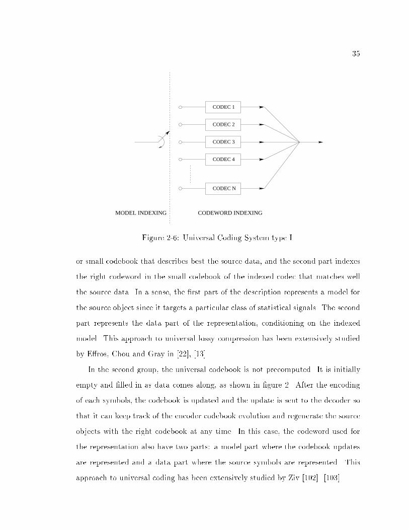
35

CODEC 1

CODEC 2

CODEC 3

CODEC 4

CODEC N

MODEL INDEXING CODEWORD INDEXING

Figure 2-6: Universal Coding System type I.

or small codebook that describes best the source data, and the second part indexes

the right codeword in the small codebook of the indexed codec that matches well

the source data. In a sense, the �rst part of the description represents a model for

the source object since it targets a particular class of statistical signals. The second

part represents the data part of the representation, conditioning on the indexed

model. This approach to universal lossy compression has been extensively studied

by E�ros, Chou and Gray in [22], [13].

In the second group, the universal codebook is not precomputed. It is initially

empty and �lled in as data comes along, as shown in �gure 2. After the encoding

of each symbols, the codebook is updated and the update is sent to the decoder so

that it can keep track of the encoder codebook evolution and regenerate the source

objects with the right codebook at any time. In this case, the codeword used for

the representation also have two parts: a model part where the codebook updates

are represented and a data part where the source symbols are represented. This

approach to universal coding has been extensively studied by Ziv [102]. [103].

36

CHANNEL DEMUX DECODER

CODEBOOK

MUXENCODER

CODEBOOK

Input data Output data

index of requestcodeword requestedcodeword requested

index of request

UPDATEMODEL DATA

TWO PART CODE

Figure 2-7: Universal Coding System type II.

index sent

index update

CODEBOOK

ENCODERInput data

CHANNELreceived index

DECODER

CODEBOOK

index update

codeword requestcodeword request

index of requested codeword

index of requested codeword

Output data

Figure 2-8: Universal Coding System type III.

The third group is similar to the second one. It forms a distinct category sim-

ply because codebook updates do not have to be sent. But it preassumes that

the encoder and decoder have agreed on systematic ways to build their codebook

respectively from incoming data. In this case, the codewords used for the represen-

tation have only one part, the data part. The model part is skipped because of the

pre-agreement between the sender and receiver on how to build the codebook from

incoming data. Extensive work on this technique has been done Zhang and Weir

[101] and also Goyal [34].

Although not highlighted in the third group, an important principle comes out

from all universal coding techniques: the separation principle between model and

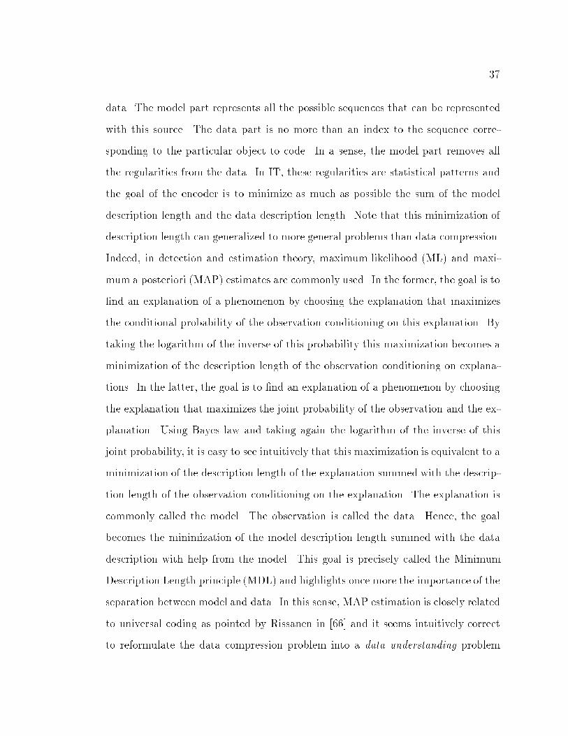
37

data. The model part represents all the possible sequences that can be represented

with this source. The data part is no more than an index to the sequence corre-

sponding to the particular object to code. In a sense, the model part removes all

the regularities from the data. In IT, these regularities are statistical patterns and

the goal of the encoder is to minimize as much as possible the sum of the model

description length and the data description length. Note that this minimization of

description length can generalized to more general problems than data compression.

Indeed, in detection and estimation theory, maximum likelihood (ML) and maxi-

mum a posteriori (MAP) estimates are commonly used. In the former, the goal is to

�nd an explanation of a phenomenon by choosing the explanation that maximizes

the conditional probability of the observation conditioning on this explanation. By

taking the logarithm of the inverse of this probability this maximization becomes a

minimization of the description length of the observation conditioning on explana-

tions. In the latter, the goal is to �nd an explanation of a phenomenon by choosing

the explanation that maximizes the joint probability of the observation and the ex-

planation. Using Bayes law and taking again the logarithm of the inverse of this

joint probability, it is easy to see intuitively that this maximization is equivalent to a

minimization of the description length of the explanation summed with the descrip-

tion length of the observation conditioning on the explanation. The explanation is

commonly called the model. The observation is called the data. Hence, the goal

becomes the minimization of the model description length summed with the data

description with help from the model. This goal is precisely called the Minimum

Description Length principle (MDL) and highlights once more the importance of the

separation between model and data. In this sense, MAP estimation is closely related

to universal coding as pointed by Rissanen in [66] and it seems intuitively correct

to reformulate the data compression problem into a data understanding problem

38

where we are seeking the best explanation for an observation of a source. This

understanding problem requires a good estimation of the machinery hidden inside

the box representing the information source and a good representation of the source

output, conditioning on this good source model.

Finite object modeling is a di�cult challenge with such a probabilistic approach.

The asymptotic nature of the de�nition of universal coding prevents us from ad-

dressing this problem in this setting. It limits signi�cantly the practical domain

of application of these ideas in media representation. Also, for visual information,

things become much more complex when we consider the HVS at the end of the

communication system. While the brain still remain a complex mysterial organ,

progress in biology have proposed valid theories approximating it with a large �-

nite state machine (or a practical computer). Indeed, electrical models for neurons

have been developed to understand the transmission of information in the brain and

they tend to support the �nite state model. This could explain why images do not

appear typical or patternless to us, although current practices in image processing

treat them as typical random events, following the guidelines provided by IT that

considers only typical sequences.

2.5. Conclusion

In this chapter, we have introduce fundamental concepts that will be used in this

thesis. We have done a quick and certainly not exhaustive survey of the �eld of lossy

universal source coding. We have �nished it by highlighting the importance of the

separation principle between model and data. In the next chapters, we will argue

that this separation will always be at the heart of the design of any coding technique.

It might not be strikingly visible in certain cases because of prior assumptions made

on the model class that is considered by the technique. For instance, the third

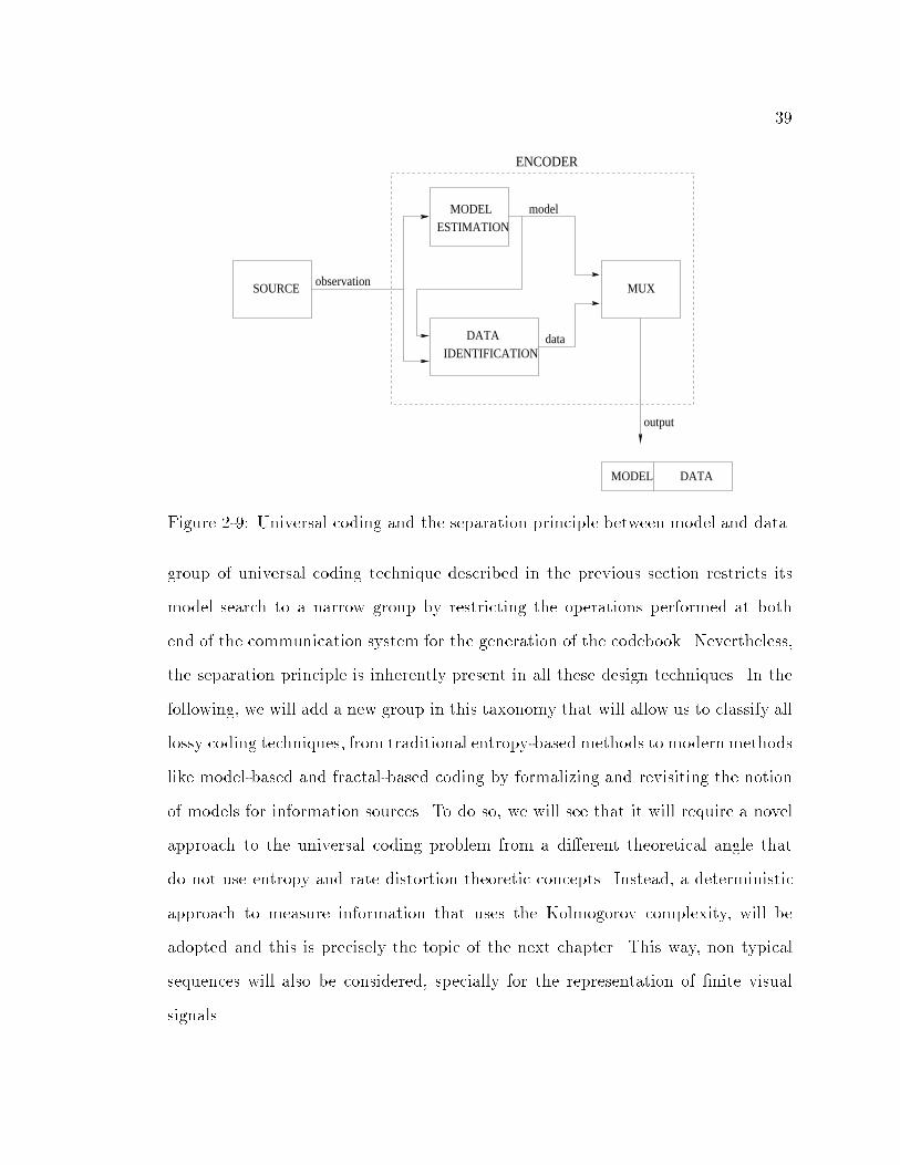
39

MODEL

MODEL DATA

DATAIDENTIFICATION

SOURCE MUX

output

data

model

observation

ENCODER

ESTIMATION

Figure 2-9: Universal coding and the separation principle between model and data.

group of universal coding technique described in the previous section restricts its

model search to a narrow group by restricting the operations performed at both

end of the communication system for the generation of the codebook. Nevertheless,

the separation principle is inherently present in all these design techniques. In the

following, we will add a new group in this taxonomy that will allow us to classify all

lossy coding techniques, from traditional entropy-based methods to modern methods

like model-based and fractal-based coding by formalizing and revisiting the notion

of models for information sources. To do so, we will see that it will require a novel

approach to the universal coding problem from a di�erent theoretical angle that

do not use entropy and rate distortion theoretic concepts. Instead, a deterministic

approach to measure information that uses the Kolmogorov complexity, will be

adopted and this is precisely the topic of the next chapter. This way, non typical

sequences will also be considered, specially for the representation of �nite visual

signals.

40

Chapter 3

Complexity Distortion Theory

3.1. Introduction

The concept of Algorithmic or Kolmogorov complexity was introduced simultane-

ously by R.J. Solomono� in [76], A.N. Kolmogorov in [44] and G. Chaitin in [11] in

di�erent settings. Solomono� was concerned with the application of Bayes's Rule

in statistics and inductive inference problems. He introduced the \Kolmogorov"

complexity as an auxiliary concept to obtain a universal a priori probability [52],

measuring the length of shortest e�ective descriptions of objects. His work provides

the theoretical foundation for the Minimum Description Length (MDL) principle.

MDL was introduced by Jorma Rissanen to tackle grave problems with density esti-

mation arising from the di�culty of �nding a way to give a constructive de�nition of

probability which would allow us to recognize it in a clear cut way. All attempts to

attach inherent probabilities to observed data have failed, as they indeed must [66]

since they require in�nite observations. This problem is even more striking when the

phenomenon under investigation is �nite. For instance, consider a �nite sequence

of zeros and ones and let's try to infer from this �nite observation a description

model. The use of time averages that estimate probabilities is hard to justify sim-

ply because there is not enough physical evidence to guarantee convergence to the

41

true distribution of the object [42]. According to the MDL principle and following

Occam's Razor principle, the best explanation would be the one that describes the

object with the shortest representation that includes the model description and the

object description with this model.

Kolmogorov studied independently shortest e�ective descriptions of individual

objects for its own sake and this is probably why the term Kolmogorov complexity

is so deployed when we refer to the complexity of an object. His work links short

descriptions to randomness and universal object distributions. It provides an inter-

esting theoretical framework where we can discuss the modeling of �nite objects.

The main idea is that an object with a short description should not be considered

random. For example the following sequence 01010101... has a structure that allows

it to be represented in a very compressed form. Randomness becomes associate to a

lack of deterministic pattern. In the following sequence, 101101100010..., it is more

di�cult to identify a deterministic pattern. Such a sequence cannot be compressed

much and is labeled random. In contrast with Shannon's information theory which

de�nes description length from randomness or probabilities, Kolmogorov complexity

theory formalized randomness from description lengths.

Chaitin's approach grew from a di�erent and much more ambitious motivation

and yielded Algorithmic Information Theory. The result of his work is a deeper

understanding of G}odel incompleteness results [31] and how they a�ect the search

for a universal mathematical theory as conceived by David Hilbert. In an attempt

to bring more light to Hilbert's dream of such a theory with no paradoxes, he came

up with the need to de�ne the amount of randomness in individual objects as did

Kolmogorov. Despite being of fundamental importance for science in general, this

approach is beyond the scope of this thesis but it illustrates once more the large

application scope of information theoretic notions.

42

In all cases, the whole theory grows from the fact that, in contrast with Shan-

non's IT, it seems very natural to de�ne the amount of information in relation to

an individual object rather than in relation to a set of objects from which the indi-

vidual objects may be selected. To formalize this individual notion of information,

a description language has to be �xed. This language must be universal to allow

the description of all conceivable objects. It also must be implementable, allowing

us to mechanically reconstruct these objects from their descriptions. The compu-

tational model used is the universal Turing Machine and this choice is justi�ed by

the Church-Turing thesis stating that the class of algorithmically computable nu-

merical functions (in the intuitive sense) coincides with the class of partial recursive

functions, or the class of functions that can be computed on a Turing machine1.

Kolmogorov Complexity has grown substantially since its introduction in [76,

44, 11]. It has concentrated, however, on lossless representations. In this chapter,

we extend this notion of complexity to lossy representations by adding a distortion

component to the mathematical picture. This extension gives rise to Complex-

ity Distortion Theory [81, 79], a uni�ed perspective for information representation

where information { within a given distortion bound { is a deterministic notion mea-

sured by the Kolmogorov complexity. We investigate the relationship between the

program-size complexity and Shannon's information measures in both the lossless

and lossy context. We show that these two frameworks predict the same results for a

large class of objects which are called algorithmically random objects. These objects

do not have deterministic patterns. For non random objects, these two approaches

diverge.

We start this chapter with a formalization of what is a programmable decoder or

a universal Turing machine and discuss the limitation of this model. We then de�ne

1See appendix A. for precise notions on recursive functions.

43

the Kolmogorov complexity and the notion of randomness tests before proposing

an equivalence between the Kolmogorov complexity and Shannon's entropy. We

extend these results to the lossy case after introducing the concept of Complexity

Distortion Function.

3.2. Universal Turing Machines

As mentioned above, the great German mathematician David Hilbert had a dream

of a universal mathematical theory, cleaned from ambiguities and paradoxes. The

idea was to establish the underlying consistency in all mathematics. His e�ort

was proved impossible by Kurt G}odel [31] and later by Alan Turing [88]. In both

cases, the conclusion was reached by constructing ambiguous statements in a very

formal language. G}odel reached this conclusion using a language very close to LISP.

Turing came up with the Turing machine, a mechanical way to generate theorems

from axioms. This machine turns out to be the accepted mathematical model for

computers. As pointed by Chaitin, it may not be wrong to think that the computer

was invented accidently in a attempt to shed light on Hilbert's dream.

The concept of Turing machine can be derived from simpler systems called �nite

automaton (FA) consisting of a �nite set of states and a set of state transitions

that occur on input symbols chosen from an alphabet, say f0; 1g. An example of

FA is shown in �gure 3-1. It is well known that the set of languages recognized

by these machines corresponds to all regular expressions [40] and languages like

NMN = f1n0m1n j n;m > 0g do not belong to this set. Indeed, this language

cannot be recognize by a �nite state system. The value of n has to be stored during

the recognition process and n being unbounded, for any �nite state system, there is

an in�nite number of large values of n for which sequences of the type 1n0m1n cannot

be recognized. Adding an in�nite memory to an FA allows it to store temporary

44

q2 q3

q1q0

Start

d

a b

c

0

01

1

0

0

1

1

00 1 1 0 1 0 0

FINITECONTROL

FINTE AUTOMATON

Input

STATETRANSITION

DIAGRAM

Figure 3-1: Finite Automaton: The top �gure shows the transition diagram ofa �nite automaton. Assuming that the initial and �nal state are both q0, thisautomaton will recognize all sequences in which both the number of 0's and thenumber of 1's is even. The example shown in the bottom will leave the automatonin state q3 at the end of the computation.

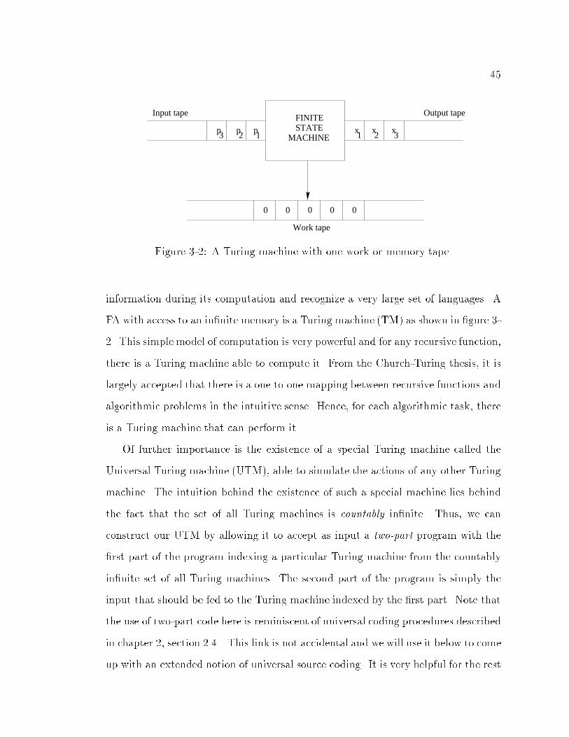
45

0 0 0 0

p p p x x xFINITESTATE

MACHINE3 2 1 1 2 3

0

Input tape Output tape

Work tape

Figure 3-2: A Turing machine with one work or memory tape.

information during its computation and recognize a very large set of languages. A

FA with access to an in�nite memory is a Turing machine (TM) as shown in �gure 3-

2. This simple model of computation is very powerful and for any recursive function,

there is a Turing machine able to compute it. From the Church-Turing thesis, it is

largely accepted that there is a one to one mapping between recursive functions and

algorithmic problems in the intuitive sense. Hence, for each algorithmic task, there

is a Turing machine that can perform it.

Of further importance is the existence of a special Turing machine called the

Universal Turing machine (UTM), able to simulate the actions of any other Turing

machine. The intuition behind the existence of such a special machine lies behind

the fact that the set of all Turing machines is countably in�nite. Thus, we can

construct our UTM by allowing it to accept as input a two-part program with the

�rst part of the program indexing a particular Turing machine from the countably

in�nite set of all Turing machines. The second part of the program is simply the

input that should be fed to the Turing machine indexed by the �rst part. Note that

the use of two-part code here is reminiscent of universal coding procedures described

in chapter 2, section 2.4.. This link is not accidental and we will use it below to come

up with an extended notion of universal source coding. It is very helpful for the rest

46

of this thesis to also view a universal Turing machine as a universal language (also

called a Turing complete language) like C or LISP, in which we can express almost

all the algorithmic task that we would like to perform.

Despite its universality, it is wrong to think that this device can solve any prob-

lem. Turing showed that there is a class of problems that cannot be solved by any

UTM. Of particular importance is the \Halting problem". Turing showed it is not

possible to design a Turing machine able to take in input any program and always

halt either in an accepting state if the input program does halt or on in a rejecting

state if the input program never halts. The consequence of the Halting problem are

devastating not only in computer science but also in coding theory and mathematics

as it shows that the existence of a class of problems that cannot be solved in an

algorithmic or mechanical logical way. It destroys Hilbert's dream.

3.3. Kolmogorov Complexity

Consider a traditional communication system where the decoder is replaced by a

universal Turing machine as shown in �gure 3-3. The codewords traveling through

the channels are now two-part programs, the �rst indexing a particular TM or al-

gorithm and the second part representing the data that the algorithm needs to

reproduce the source message. This communication system follows our natural way

of conceiving communications. Indeed, humans do communicate using languages

with strict syntactic and grammatical rules. These languages di�er from computer

languages simply because of their domain of application and their ambiguity but the

idea behind their use is the same. In such a communication setting, it seems natural

to de�ne the amount of information in an object by the length of its shortest de-

scription in the language. This approach yields directly to the notion of Kolmogorov

complexity.

47

SOURCE ENCODER DECODER USER

NOISE

SOURCE

original message

Finite State

MachineInput tape Output tape

Work tape

received program + dataprogram + data

Figure 3-3: The programmable communication system. Notice that two-part codesrepresenting algorithms and data are sent through the channel.

48

3.3.1 Individual Information Measure

The plain Kolmogorov complexity of sequence xn1 is equal to the length of the

shortest program written for a Turing machine (TM), that computes xn1 and halts.

Following the equivalence between TM's and recursive functions as discussed in

Appendix A., we can formally de�ne the Kolmogorov complexity as follows:

De�nition 1 Let F be an arbitrary partial recursive function. Then the complexity

of the sequence x 2 A with respect to F is:

KF (x) =

8><>:

minfl(p) : F (p) = xg;

1 if 8p 2 A F (p) 6= x

The sequence p for which F (p) = x is called the code or program or short descrip-

tion for x. De�nition 1 was proposed by Kolmogorov in [44]. It is often called the

plain Kolmogorov complexity. Although more suitable for information understand-

ing than the ensemble measure proposed by Shannon, the Kolmogorov complexity

as de�ned above is not completely satisfactory. This information measure is sub-

additive only up to a logarithmic term. Also, it is not monotonic over pre�xes2.

Intuitively the complexity of the concatenation xy of two strings x and y should

always exceed the complexity of x. It is not the case with the plain complexity3.

Another problem surfaces when we try to associate a probability measure with K.

By de�ning P (x) =P2�l(p), the sum being taken over all inputs p for which the as-

sumed computer output x and halts, we would like P (:) to be a probability measure

to have a better formalism for Solomono�'s induction problems. Unfortunately, this

summation diverges4. One way to solve these problems except the non monotonicity

2See example 2.5 in [52].3See example 2.10 in [52].4See [52], p 170.

49

over pre�xes is to used the pre�x complexity measure introduced by Levin, Gacs

and extended by Chaitin. In this case, programs are constrained to be pre�x free

and Kraft's inequality [52, 15] can be applied to associate a probability measure to

K. In this thesis, we use the pre�x complexity for simplicity, although the main

results proposed do hold for the other variants of Kolmogorov complexity.

De�nition 2 Let F be an arbitrary partial recursive function with a pre�x domain5.

Then the pre�x complexity of the sequence x 2 A with respect to F is:

CF (x) =

8><>:

minfl(p) : F (p) = xg;

1 if 8p 2 A F (p) 6= x

Theorem 1 There exists a partial recursive function F0 (called optimal) such that

for any other partial recursive function G,

CF0(x) � CG(x) +O(1) (3.1)

Proof: See [44].

2

The optimal function is also called the universal function. The intuition behind

this theorem is the existence of a universal computer, or UTM, able to simulate the

actions of any other computer. Since Turing machines are e�ectively enumerable,

a possible description for x is the code for x on G preceded by the index or G}odel

number of G in the e�ective enumeration of Turing machines. The theorem follows

naturally from this construction. As a result, we will drop the subscript referring to

the partial recursive function and use C(x) = CF0(x) as a notation for the complexity

of sequence x.

5A pre�x domain is a set of sequences where no sequence is the proper pre�x of another.

50

De�nition 3 The conditional complexity of a sequence x given the knowledge of

another sequence y is

C(x j y) =

8><>:

minfl(p) : F0(p; y) = xg;

1 if 8p 2 A F0(p; y) 6= x

We have dropped the subscript referring on the partial recursive function used in

the de�nition because theorem 1 does hold in this case for exactly the same reasons

mentioned above in the unconditional case.

Theorem 2 There is a constant c, such that for all x and y,

C(x) � l(x) + c (3.2)

C(x j y) � C(x) + c (3.3)

Proof: See [52].

2

The following theorem is a negative result known as the Noncomputability theorem

[52].

Theorem 3 C is not partial recursive.

Proof: See [52], [105].

2

It is a negative results since it proves that any attempt to compress maximally

sequences cannot be performed on a TM. It is a natural manifestation of the Halting

problem. It prevents us from hoping to �nd a mechanical way to �nd shortest

representations of objects. Fortunately, the next theorem states that it is possible

to approximate C.

51

Theorem 4 There is a total recursive function �(t; x), monotonic decreasing in t,

such that

limt!1

�(t; x) = C(x) (3.4)

Proof: According to [105], this theorem is due to Kolmogorov. Its proof can be

found in [105] and [52]. Since the proof hints at how computational resource bounds

at the decoding end remove the Halting problem, we reproduce it here. For each

value of t, it is possible to construct a pre�x Turing machine that runs the reference

Turing machine �xed in theorem 1 for no more than t steps on each program with

length at most l(x)+ c. We de�ne (t; �) as the partial recursive function computed

by this Turing machine. If for some input programs p, the computation halts with

output x, then we de�ne �(t; x) = minfl(p) : (t; p) = xg. Else, �(t; x) = l(x) + c.

Clearly, �(t; x) is recursive, total6, and non increasing with t. Also, the limit in

equation 3.4 exists since for each x, there is a t such that the reference Turing

machine halts and outputs x after t steps starting with input p with7 l(p) = C(x).

2

Although we can approximate C(x) from above, it does not mean that we can

decide whether �(t; x) = C(x) or not. In more intuitive words, the approximation

gets closer and closer to C but it is impossible to know how close it gets. Since

�(t; x) is recursive, it becomes possible to introduce computational resource bounds

in de�nitions 3.3.1 and 3 and obtain a recursive measure of information.

De�nition 4 [52] Let �t;s be a partial recursive function computed by a Turing

machine such that for any x 2 B, the computation of �t;s(x) requires less than

6Every �nite x has a value assigned to it by �.7Since objects are �nite, there is a value t� corresponding to the number of steps the optimal

description for x (with length equal to K(x)) takes when it is placed in input on the referenceTuring machine.

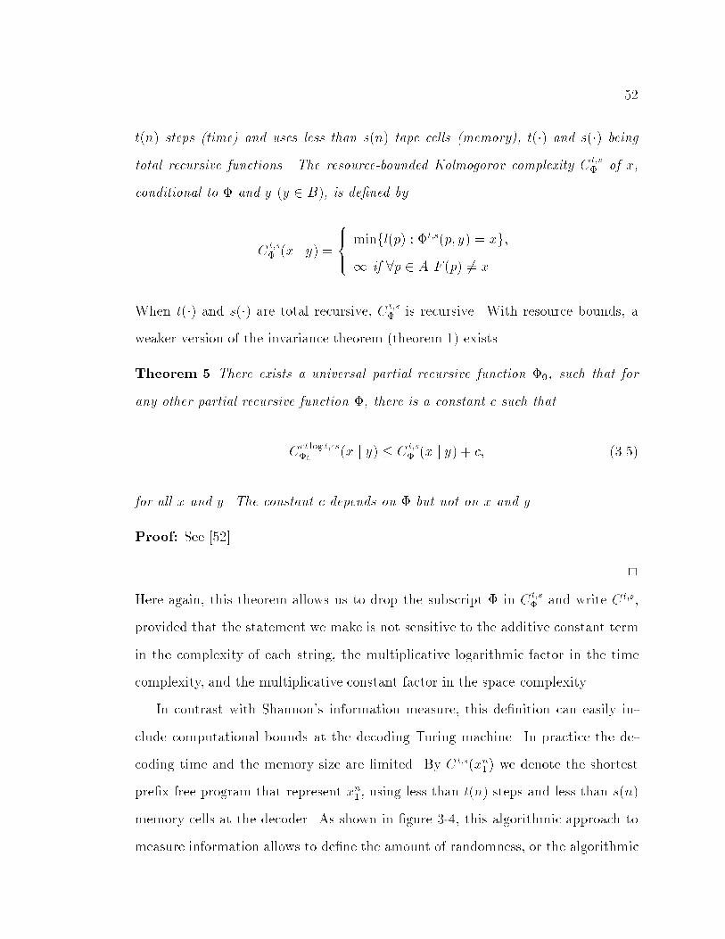
52

t(n) steps (time) and uses less than s(n) tape cells (memory), t(�) and s(�) being

total recursive functions. The resource-bounded Kolmogorov complexity C t;s� of x,

conditional to � and y (y 2 B), is de�ned by

C t;s� (x j y) =

8><>:

minfl(p) : �t;s(p; y) = xg;

1 if 8p 2 A F (p) 6= x

When t(�) and s(�) are total recursive, C t;s� is recursive. With resource bounds, a

weaker version of the invariance theorem (theorem 1) exists.

Theorem 5 There exists a universal partial recursive function �0, such that for

any other partial recursive function �, there is a constant c such that

Cct log t;cs�0 (x j y) � C t;s

� (x j y) + c; (3.5)

for all x and y. The constant c depends on � but not on x and y.

Proof: See [52].

2

Here again, this theorem allows us to drop the subscript � in C t;s� and write C t;s,

provided that the statement we make is not sensitive to the additive constant term

in the complexity of each string, the multiplicative logarithmic factor in the time

complexity, and the multiplicative constant factor in the space complexity.

In contrast with Shannon's information measure, this de�nition can easily in-

clude computational bounds at the decoding Turing machine. In practice the de-

coding time and the memory size are limited. By C t;s(xn1) we denote the shortest

pre�x free program that represent xn1 , using less than t(n) steps and less than s(n)

memory cells at the decoder. As shown in �gure 3-4, this algorithmic approach to

measure information allows to de�ne the amount of randomness, or the algorithmic

53

probability in individual objects (See [76]), in contrast with Shannon's Information

Theory (IT) which uses randomness or probability theory to de�ne information.

3.3.2 Randomness Tests

In contrast with Shannon's ensemble information measure which is based on proba-

bilities, the Kolmogorov complexity is an individual information measure. Another

major di�erence between these two measures of information is in the motivation

behind their introduction. Shannon's measure was introduced to tackle a communi-

cation problem and is derived from probability theory. The main motivation behind

the introduction of the Kolmogorov complexity is to characterize the amount of

randomness in individual objects. In this case, an information theoretic approach

is used to derive a theory of randomness. As explained in [43], random sequences

possess three properties:

1. being typical: This property was pointed out by Martin-L}of [54]. A random

sequence is typical as opposed to be very special like an in�nite sequence of

zeros. The property of being typical is identical to the property of belonging to

any reasonable majority. More formally, the set of random sequences should

have measure 1. As a result, when we choose some object at random, we are

almost sure that the object belongs to this majority and we expect to get a

typical sequence. In traditional information theory, typical sequences x are the

one with probability p(x) close to 2�l(x)H , H being the entropy of the source

(assuming that this entropy exists). The Shannon-McMillan-Breiman theorem

shows that this set of sequences has measure one for stationary ergodic sources.

2. being chaotic: This property was pointed out by Kolmogorov. A random

sequence is chaotic in the sense that it has no simple law governing the alter-

nation of its terms. Traditional information theoretic notion of typicality fails

54

From Complexities to Probabilities

From Probabilities to Complexities

COMPLEXITIES PROBABILITIES

STOCHASTICAPPROACH(SHANNON)

INDIVIDUALAPPROACH

(KOLMOGOROV)

Figure 3-4: Duality between Shannon's entropy and Kolmogorov complexity.

to capture this8. It is very easy to think of a typical sequence according to IT

but with a very short mechanical description, capturing all the regularities in

this sequence.

3. being stochastic: This property was pointed out by von Mises. The frequency

of zeros in the beginning segments of a random sequence (assuming a Bernoulli

12 process), must converge to

12 . And this e�ect must be observed not only for

the entire sequence but also for any of its properly chosen subsequences. The

term properly chosen is here to guarantee that there are no gambling strategy.

A player betting in �xed amounts on the outcomes of any random sequence

after seeing all the previous outcomes cannot obtained any gain in the long

run.

8For example, assume a Bernoulli source with parameter p = 1

2, then x = 010101::: will have

an empirical probability close to 2nH for large n although this sequence is quite regular.

55

There have been many unsuccessful attempts to formalize these properties. In 1966,

Martin-L}of [54] gave a de�nition of random sequences based on Kolmogorov com-

plexity and on statistical tests verifying all three properties for in�nite sequences.

An interesting aspect of this work is that it also applies to �nite sequences by using

levels of randomness. All statistical tests are e�ective such that they can compute

at each level of randomness which sequences should be labeled not random. This

observation yields de�nitions of randomness for individual sequences. These precise

statements are presented in appendix B.. The reader who is not familiar with these

notions should consult appendix B. or [52] before going any further in this thesis.

3.4. Equivalence with Information Theory

Despite their conceptual di�erences, the Kolmogorov complexity and Shannon's en-

tropy are equivalent for a very wide class of information sources. In this section,

we establish these links and identify precisely the set of sequences where the equiv-

alence does not hold. This set corresponds to non random sequences with strong

deterministic or mechanical patterns.

3.4.1 Fundamental Theorem

Levin and Zvonkin were the �rst one to formulate an equivalence between Shannon's

entropy rate and the Kolmogorov complexity. In [105] the following theorem is

formulated without proof:

Theorem 1 For a stationary ergodic source (A;A; �) with a recursive probability

measure �,

limn!1

C(xn1)

n= H(�); xn1 2 An �-a.s. (3.6)

56

In this theorem, the ergodic decomposition of stationary process allows us to drop

the ergodicity assumption if we allow the introduction of an expectation term on

the Kolmogorov complexity. The importance of this result cannot be overstated as

it clearly shows that despite introducing a mechanical structure at the decoding end

of Shannon's classical system, we do not lose much in terms of performance. Fur-

thermore, the proposed proof will de�ne precisely the null set of in�nite sequences

where the equivalence does not hold. For �nite sequences, we will derive upper

bounds on the measure of that set. A formal proof of this result is presented below

but �rst, we present the intuition behind this result.

Intuition behind Theorem 1

The equivalence between Shannon's probabilistic approach and Kolmogorov's deter-

ministic approach holds for a large class of sequences that are called algorithmically

random. Sequences from this set do not exhibit any form of regularity that could

be exploited by a computer program. Hence, the best way to represent them is with

a probabilistic approach. If � is recursive, there is a mechanical way to describe it.

In this case, a sequence can be described with a computer program specifying �,

followed by an e�cient entropy coding technique. From such a code construction,

we can show that the Kolmogorov complexity of an in�nite observation of a sta-

tionary source with recursive probability measure is upper bounded by the length

of this simple two-part description. Since the description of the probability measure

is independent of the observation length, and since the length of the second part of

the code is close to nH, H being the entropy rate of the source, we claim that

lim supn!1

C(xn1)

n� H(�); xn1 2 An �-a.s. (3.7)

Note that in the derivation of this upper bound, we do not use Shannon's source

coding theorem that predicts the existence of codes operating at rates close to the

57

entropy rate for stationary ergodic processes. We cannot use it here simply because

Shannon's source coding theorem does not make any computational assumptions on

the decoding device n. Hence, it does not guarantee that this function is actually

recursive. Instead, we use the concept of Markov types [73, 18]9 with a known coding

procedure [73] and use the recursive assumption on the source probability measure

to come up with a code that can actually be decoded on a UTM. Also, note that

the two-part structure of the code which is a key characteristic of universal coding

techniques. The �rst part of the code describes the model used, here a probabilistic

model (the source distribution). The second part of the code describes the actual

data, the observation, with help from the probabilistic model described in the �rst

part. To �nish the proof of the theorem 1, it remains to show that:

lim infn!1

C(xn1)

n� H(�); xn1 2 An �-a.s. (3.8)

This is done by proving that the setnx 2 Atyp : lim infn!1

C(xn1)

n< H(�)

ois a null

set, where Atyp is the set of sequences verifying the Shannon-McMillan-Breiman

theorem. In other words, we have to prove that according to the source probability

measure, it is very unlikely to have a sequence with Kolmogorov complexity below

the length of its Shannon-Fano code. This conclusion is obtained directly with

a universal randomness test linking Shannon-Fano code lengths with Kolmogorov

complexities. Shannon-Fano code lengths are then linked to the entropy rate of

the source via the Shannon-McMillan-Breiman theorem proved by Breiman in the

almost sure sense.

9The reader who is not familiar with Markov types should consult appendix C. or [73]. For amore general a complete treatments on types, she should refer to [16].

58

3.4.2 Proof of Fundamental Theorem

We proceed with the proof of theorem 1. In the �rst part, we show the following

lemma:

Lemma 1 For a stationary ergodic source (A;A; �) with a recursive probability

measure �,

lim supn!1

C(xn1)

n� H(�); xn1 2 An �-a.s. (3.9)

Proof of lemma 1:

For a lossless representation, we can represent the sequence xn1 by the following

two-part code proposed in [73]:

1. The index of the Markov k-type of xn1 is transmitted.

2. The index of xn1 in the type class Tk(xn1) is transmitted.

The �rst part of the code requires only m = o(n) if k = b12logjA0j nc. The second

part converges to n times the entropy rate as proved in [73]:

limn!1

l(�n(xn1))

n= H(�), �-a.s. (3.10)

�n being the encoding function described above. Since the proposed code is pre�x

free [73], it is a valid program for a pre�x Turing machine. Furthermore, the decod-

ing operations are clearly recursive meaning that there is a pre�x Turing machine

able to decode this code. This machine has to reproduce all sequences with Markov

type equal to the one that has been sent and then the machine indexes the right

sequence from the second part of the code. Therefore, we conclude that:

C(xn1) � l(n(xn1 )) (3.11)

59

and also that:

lim infn!1

C(xn1)

n� lim sup

n!1

C(xn1)

n� H(�), �-a.s. (3.12)

proving lemma 1.

2

To prove theorem 1, what remains to be done is to prove the following lemma:

Lemma 2 For a stationary ergodic source (A;A; �) with a recursive probability

measure �,

lim infn!1

C(xn1)

n� H(�); xn1 2 An �-a.s. (3.13)

Proof of lemma 2:

Lemma 1 in appendix B. implies that for any x 2 A1, if �0(x j �) <1 then x

is random with respect to �. In this case, Let � = �0(x j �). For any n 2 N ,

�C(xn1 j �)� log2 �(xn1 )

n�

�

n(3.14)

Since � is assumed recursive, C(xn1 j �) � C(xn1) + O(1), the constant term being

present to take into account the length of the description of �.

� log2 �(xn1 )

n�

�

n+C(xn1 j �)

n�

�

n+C(xn1) +O(1)

n(3.15)

In the limit as n grows, we get

lim infn!1

� log2 �(xn1 )

n� lim inf

n!1

C(xn1)

n(3.16)

60

the last equation holds for any � random sequences and this set has �-measure 1.

Therefore, the set

(x 2 A1 : lim inf

n!1

C(xn1)

n< � lim inf

n!1

log2 �(xn1 )

n

)(3.17)

is a null set. Recall the Shannon-McMillan-Breiman theorem proving that for a

�nite-valued stationary ergodic process fXng with measure �,

�1

nlog �(X0; � � � ;Xn�1)! H(�) (3.18)

�-almost surely as n ! 1. Since the intersection of a null set with another set

is still a null set, we can use the Shannon-McMillan-Breiman theorem to conclude

that for a stationary ergodic source,

�

(x 2 A1 : lim inf

n!1

C(xn1)

n< � lim

n!1

log2 �(xn1 )

n

)= �

(x 2 Atyp : lim inf

n!1

C(xn1)

n< H(�)

)= 0

(3.19)

Consequently,

lim infn!1

C(xn1)

n� H(�); �-a.s.

2

From lemma 1 and 2, it is trivial to show that limn!1C(xn

1)

nexists10 �-almost

surely and is then equal to H(�), proving theorem 1.

2

10It is easy to construct a sequence with

lim supn!1

C(xn1 )

n6= lim inf

n!1

C(xn1 )

n:

The limit exists at least on a set of measure one, namely the set of random sequences. See [52]

61

3.5. Complexity Distortion Function

In this section, we extend Kolmogorov Complexity Theory to the lossy case where

distortion is allowed given rise to \Complexity Distortion Theory" (CDT). As men-

tioned before, Rate Distortion Theory (RDT) does not make any assumptions on

the structure of the decoding function n. The main di�erence between CDT and

RDT is the restriction of n to the set of partial recursive function. As a conse-

quence, each function n can be realized by a Turing machine. In this lossy setting,

it is more natural to measure information with an extension of the Kolmogorov

complexity to the semifaithful case. To introduce it, we contrast it with the RDF.

Recall the sphere covering approach used in the de�nition of the operational rate

distortion function in chapter 2. It was interpreted as the minimum number of balls

of radius D needed to cover (almost surely) the space of all sequences of length n for

very large values of n. The complexity distortion function can be introduced in the

same lines. In a D-ball centered this time around xn1 , let QD(xn1) be the sequence in

An with the smallest Kolmogorov complexity. If we have many sequences inside the

ball, we pick the closest one to xn1 , according to dn. If we still have more than one

candidate, we list them in a lexicographic order and arbitrarily pick the sequence

with the smallest index in the list.

QD(xn1) = arg min

yn12An:dn(xn1 ;y

n1)�D

C(yn1 ) (3.20)

De�nition 5 The complexity distortion function is de�ned as:

CD(x) =C(QD(x))

l(x)(3.21)

There are two striking di�erences between the rate distortion function and the com-

plexity distortion function:

62

1. The complexity distortion function is a deterministic quantity that does not

rely on any probabilistic assumptions, in contrast with the rate distortion

function relying on the probability measure associated to the source.

2. The complexity distortion function describes the best element inside a D-ball

and does not ignore the information content. The rate distortion function

does not describe the content of any elements of the D-ball. It simply indexes

these balls following the general information theoretic belief that the actual

meaning of messages is irrelevant to the communication problem [70]. Note

that this indexing is done from the knowledge of source distribution at both

end of the communication system. This knowledge describes the universe of all

possible messages, a piece of information which is not required in complexity

distortion theory.

This \sphere covering" approach emphasizes how CDT generalizes RDT. It has some

strong connections with Vector Quantization (VQ) and sets the stage up for a new

approach to universal coding that will be presented in the next chapter.

3.6. Equivalence with Rate Distortion Theory

This section extends theorem 1 to the lossy case and closes the circle of media

representation techniques shown in �gure 3-5, from traditional stochastic modeling

approach shown on the left side of the picture, to modern deterministic modeling

approach as show on the right side of the �gure.

3.6.1 Extended Fundamental Theorem

The extended fundamental theorem is formulated as follows:

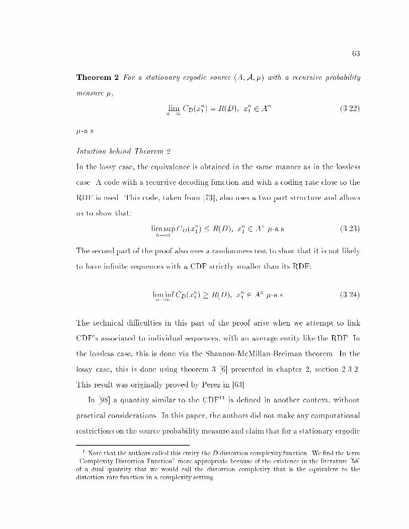
63

Theorem 2 For a stationary ergodic source (A;A; �) with a recursive probability

measure �,

limn!1

CD(xn1) = R(D); xn1 2 An (3.22)

�-a.s.

Intuition behind Theorem 2

In the lossy case, the equivalence is obtained in the same manner as in the lossless

case. A code with a recursive decoding function and with a coding rate close to the

RDF is used. This code, taken from [73], also uses a two part structure and allows

us to show that:

lim supn!1

CD(xn1) � R(D); xn1 2 An �-a.s. (3.23)

The second part of the proof also uses a randomness test to show that it is not likely

to have in�nite sequences with a CDF strictly smaller than its RDF:

lim infn!1

CD(xn1) � R(D); xn1 2 An �-a.s. (3.24)

The technical di�culties in this part of the proof arise when we attempt to link

CDF's associated to individual sequences, with an average entity like the RDF. In

the lossless case, this is done via the Shannon-McMillan-Breiman theorem. In the

lossy case, this is done using theorem 3 [6] presented in chapter 2, section 2.3.2.

This result was originally proved by Perez in [63].

In [98] a quantity similar to the CDF11 is de�ned in another context, without

practical considerations. In this paper, the authors did not make any computational

restrictions on the source probability measure and claim that for a stationary ergodic

11Note that the authors called this entity the D-distortion complexity function. We �nd the term\Complexity Distortion Function" more appropriate because of the existence in the literature [58]of a dual quantity that we would call the distortion complexity that is the equivalent to thedistortion rate function in a complexity setting.

64

INFORMATION THEORY KOLMOGOROV COMPLEXITY

RATE DISTORTION THEORY COMPLEXITY DISTORTION THEORY

Figure 3-5: The circle of media representation theories (the bottom-right box aswell as its associated arrows, establishing its relationship with other theories, areintroduced in this thesis).

source, the rate distortion function and the complexity distortion function are almost

surely equivalent. We present an alternative simpler proof of this result for recursive

sources which is more constructive, and explains why the problem of coding �nite

objects, under computational resource bounds �ts better in this algorithmic setting.

In contrast with the proof proposed in [98] and [99] for the lossless case, the proof

here does not use the variable length source coding theorem [70] nor its extension to

the lossy case simply because these theorems are not constrained by any recursive

assumptions12. Furthermore, we highlight the separation principle between model

and data [92] by using two-part codes. This approach provides very useful hints for

the design of codecs that will be discussed in the next chapter.

3.6.2 Proof of Extended Fundamental Theorem

The proof is done in two parts. In the �rst part, we show the following lemma:

12These theorems cannot be used to compute lower bounds on Kolmogorov complexities becausethey predict existence of codes that may or may not be decodable by any recursive function if thesource is governed by a probability law that may not be recursive, as assumed in [98, 99].

65

Lemma 3

lim supn!1

CD(xn1 ) � R(D); xn1 2 An �-a.s. (3.25)

Proof of Lemma 3: To encode xn1 e�ciently, recall that a D-cover of a set S � An

is a collection G � An such that every sequence in S is within D of some member of

G. For a lossy representation, the sequence xn1 can be represented by the following

two part code proposed in [73]:

1. The index of the Markov k-type of xn1 is transmitted.

2. Choose a D-cover Gk(Tk(xn1 )) of least cardinality among allD-covers of Tk(xn1).

The second part of the code is then an address of an element of Gk(Tk(xn1)) that

is within D of xn1 . Clearly, this address requires at most log2 j Gk(Tk(xn1)) j.

We already mentioned in section 3.4.2 that the �rst part of the code requires only

m = o(n) if k = b12logjA0j nc. It is shown in [73] that the ratio of the length of the

second part of the code to n converges almost surely to the rate distortion function

of the source.

Lemma 4

limn!1

l(�n(xn1))

n= R(D) a.s. (3.26)

�n being the encoding function corresponding to the code construction presented

above.

See [73] for a proof of this result. This code is pre�x free [73] and is a valid program

for a pre�x free Turing machine. The decoding operations are clearly recursive

since the probability measure of the source is assumed recursive. As a result, we

can construct a Turing Machine able to take this code as input and able to output

66

a sequence yn1 2 An with dn(xn1 ; yn1 ) � D. Consequently, we have shown that:

lim supn!1

CD(xn1) � R(D); xn1 2 An �-a.s. (3.27)

2

In the second part of the proof of theorem 2, we show the following lemma:

Lemma 5

lim infn!1

CD(xn1) � R(D); xn1 2 An �-a.s. (3.28)

Proof of lemma 5: To get this result, we start by designing a universal test for

in�nite sequences of the reproduction alphabet.

Lemma 6 � is recursive and the function

�1(! j �) = sup!2�y

f�C(y j �) � log2 �(y)g (3.29)

is a universal integral �-test.

Proof of lemma 6: This result is similar to the test used in 3.4.2. The only

thing that we have to show here is that � is recursive. To do so, note that � is a

probability measure induced by the measurement QD(�), from A� to A�. Since � is

recursive by assumption and QD is enumerable from theorem 4 in this chapter, then

� is enumerable and there exists a recursive function g(k; y), k 2 N , y 2 A�, non

decreasing in k such that limk!1 g(k; y) = �(�y). Since � is a probability measure,

we can compute an approximation �k of � from below such thatP

x:l(x)=l(y) �k(�x) >

1 � �, � being arbitrary. This means that j �(�y) � �k(�y) j< �, for all y and � is

recursive13. To show that �1 is a universal test, we just have to invoke lemma 1,

13See example 4.3.2 in [52] for an identical argument. Note that the authors have a conventionreplacing cylinders by the actual sequences, as explain in section 4.2.

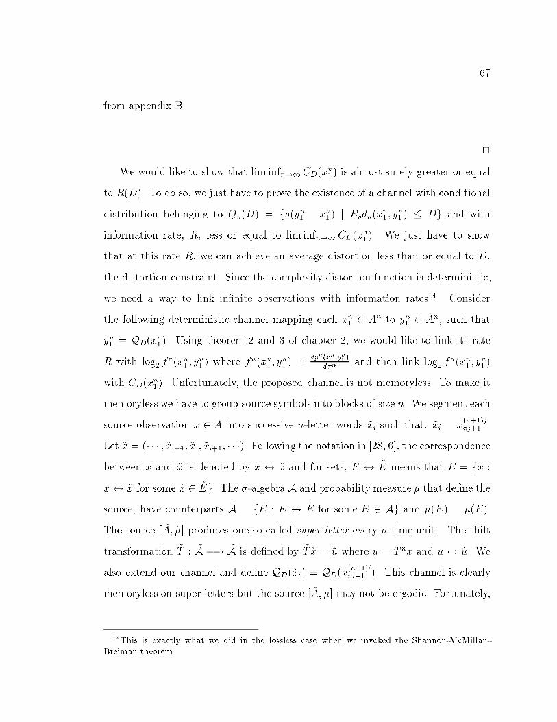
67

from appendix B..

2

We would like to show that lim infn!1 CD(xn1) is almost surely greater or equal

to R(D). To do so, we just have to prove the existence of a channel with conditional

distribution belonging to Qn(D) = f�(yn1 j xn1 ) j Epdn(xn1 ; yn1 ) � Dg and with

information rate, R, less or equal to lim infn!1 CD(xn1). We just have to show

that at this rate R, we can achieve an average distortion less than or equal to D,

the distortion constraint. Since the complexity distortion function is deterministic,

we need a way to link in�nite observations with information rates14. Consider

the following deterministic channel mapping each xn1 2 An to yn1 2 An, such that

yn1 = QD(xn1). Using theorem 2 and 3 of chapter 2, we would like to link its rate

R with log2 fn(xn1 ; y

n1 ) where fn(xn1 ; y

n1 ) =

dpn(xn1;yn1)

d�nand then link log2 f

n(xn1 ; yn1 )

with CD(xn1). Unfortunately, the proposed channel is not memoryless. To make it

memoryless we have to group source symbols into blocks of size n. We segment each

source observation x 2 A into successive n-letter words ~xi such that: ~xi = x(n+1)jnj+1 .

Let ~x = (� � � ; ~xi�1; ~xi; ~xi+1; � � �). Following the notation in [28, 6], the correspondence

between x and ~x is denoted by x $ ~x and for sets, E $ ~E means that E = fx :

x$ ~x for some ~x 2 ~Eg. The �-algebra A and probability measure � that de�ne the

source, have counterparts ~A = f ~E : E $ ~E for some E 2 Ag and ~�( ~E) = �(E).

The source [ ~A; ~�] produces one so-called super letter every n time units. The shift

transformation ~T : ~A �! ~A is de�ned by ~T ~x = ~u where u = T nx and u$ ~u. We

also extend our channel and de�ne ~QD(~xi) = QD(x(n+1)ini+1 ). This channel is clearly

memoryless on super letters but the source [ ~A; ~�] may not be ergodic. Fortunately,

14This is exactly what we did in the lossless case when we invoked the Shannon-McMillan-Breiman theorem.

68

it can be decomposed into ergodic modes15 as follows: De�ne a non null invariant

set G 2 ~A as a set that both satis�es ~�(G) > 0 and ~T (G) = G. A non null invariant

set that cannot be partitioned into two non-null invariant sets is called an ergodic

mode.

Lemma 7 Let [A;�] be a time-discrete, stationary, ergodic source. Then the asso-

ciated source [ ~A; ~�] of n-dimensional super letters can be decomposed into m ergodic

modes, E00; � � � ; E

0m�1, where m is a divisor of n. If 0 � j;� m� 1 and j 6= k, then

~�(E0j) =

1m

and ~�(E0j

TE0k) = 0.

See [6] for a proof of this result. In each of these modes, we compute the information

rate that is achieved when the channel is deterministic and modeled by the function

~QD(�). Consider the sources [ ~A; ~�i], i = 0; � � � ;m� 1, de�ned by

~�i(C0) = m~�(C 0

\E0i); C

0 2 A0

where E0i is the ith ergodic mode of [ ~A; ~�]. It follows from lemma 7 that each of

these sources are ergodic with respect to the super letter shift transformation ~T and

theorem 3 can be used to get an expression for the information rate, ~Ri obtained

by passing the output of these sources through the deterministic channel ~QD. Let

f ti (~xt1;

~yt1) be the Radon Nikodym derivative of ~pti with respect to ~�ti. Then by

theorem 2 and 3 in chapter 2,

limt!1

log2 fti (~xt1;

~yt1)

t= ~Ri; ~pi-a.s. (3.30)

15See [28] for a brief but excellent discussion on ergodic modes, in a context similar to the onethat we have here.

69

From the de�nition of f ti , for any s 2 N , since log2 is continuous on R+ and right

continuous at 0,

log2 fsi ( ~x

s1; ~y

s1) = log2 lim

u!1

psi (Fu)

�si (Fu)= lim

u!1(log2 p

si (Fu)� log2 �

si (Fu)) (3.31)

where fFug is a sequence of Borel sets converging regularly16 to ( ~xs1; ~ys1). Using

De Possel's theorem [74] we can restrict the sequence fFug to be nested: Fu+1 �

Fu; u > 0. Therefore, using the continuity from above property of �nite measures

[26],

log2 fsi ( ~x

s1; ~y

s1) = log2 ~p

si ( ~x

s1; ~y

s1)� log2 ~�

si ( ~x

s1; ~y

s1); ~psi -a.s.,

and,

log2 fsi ( ~x

s1; ~y

s1) = log2 ~�

si ( ~x

s1) + log2 ~r

si ( ~y

s1 j ~x

s1)� log2 ~�

si ( ~x

s1)� log2 ~�

si ( ~y

s1) ~p

si -a.s.

Since ~ys1 = ~QD( ~xs1), log2 ~ri( ~ys1 j ~x

s1) = 0 we obtain:

log2 fs( ~xs1; ~y

s1) = � log2 ~�

si ( ~y

s1) ~p

si -a.s. (3.32)

~�i is clearly recursive17. Recall lemma 6. For any ~y, if �1(~y j ~�i) < 1, then ~y is

random with respect to ~�i. Let �i = �1(~y j ~�i). For any s 2 N ,

�C( ~ys1 j ~�i)� log2 ~�si ( ~y

s1)

s�

�is

16Please see [74].17We proved that � is recursive and know that for almost all y, �(y) is either zero or equal to

�i(y), if y 2 Ei or not. If y 2 Ei, ~�i is equivalent to �, a recursive set function.

70

Since ~�i is recursive, in the limit as s!1, we get:

lim infs!1

� log2 ~�si ( ~y

s1)

s� lim inf

s!1

C(~ys1)

s� lim inf

s!1

C(ysn1 ) + log2 n+ c

s(3.33)

c being a constant. The last inequality holds because ~ys1 can be computed from

ysn1 using a �nite program of length less than c + log2 n, c being a constant. Since

equation 3.33 holds for ~�i random sequences forming a set of ~�i-measure 1, the set

(y 2 A1 : lim inf

s!1

C(ysn1 )

s< � lim inf

s!1

log2 ~�si ( ~y

s1)

s

)

is a null set according to both measures ~�i and ~pi. Therefore, we conclude that:

� lims!1

log2 ~�si ( ~y

s1)

s� lim inf

s!1

C(ysn1 )

s; ~pi-a.s. (3.34)

Since ~ys1 = ~QD( ~xs1), ~psi ( ~x

s1; ~y

s1) = ~�si ( ~x

s1),

lims!1

log2 fsi ( ~x

s1; ~y

s1)

s� lim inf

s!1nCD(x

sn1 ); ~�i-a.s. (3.35)

and from equation 3.30,

Ri = limt!1

log2 fti (~xt1;

~yt1)

nt� lim inf

t!1CD(x

nt1 ); ~�i-a.s. (3.36)

where Ri =~Ri

n. From the subadditive ergodic theorem, it is easily veri�ed that

lims!1 CD(xs1) is �-almost surely a constant. Consequently, the Ri's are also �-

almost surely upper bounded by this constant that we denote R. Note that R can

be easily achieved by the source [A;�] at distortion level D. To see this, note that

~Ri � ~R1i (D), the �rst order rate distortion function for the source [ ~A; ~�i], since

at the rate ~Ri the distortion constraint D is respected from the de�nition of ~QD.

71

Hence, from theorem 5 chapter 2, for t su�ciently large, there exists a D-admissible

code for [ ~A; ~�i], of blocklength t in super letters and size

Ki � 2t(~R1i (D)+�) � 2t(

~Rmax+�) (3.37)

where ~Rmax = supi ~Ri. Consider the following code obtained by combining the

di�erent m ergodic modes. Each ergodic mode can be encoded at the rate ~Ri by

using QD(�) yielding a code denoted Bi18. These Bi's can be combined into a \giant"

code, B, that is D-admissible and with rate less or equal to R by taking their union

over m. Clearly, the rate of B, denoted RB, is upper bounded by:

RB =log2 j B j

tn�

log2(m2t(~Rmax+�))

tn=

log2m+ t ~Rmax + t�

tn(3.38)

for t large enough. Therefore since � is arbitrary, and since~Rmax

n= supiRi �

R �-a.s., by letting n ! 1, we have shown that RB � R, almost surely. Fur-

thermore, since RB is achievable with an average distortion less than D, so is R,

we conclude that R � R(D) and also that lim infm!1 CD(xm1 ) � R(D), �-almost

surely, .

2

The proof of theorem 2 follows from lemma 3 and lemma 5.

2

18This code is suggested in [6, 28] but not used in the proof of the fundamental theorem forstationary ergodic source. The reason is that the Ri used in this theorem are not constant.Therefore, a simple union of the codes Bi described below would yield upper bounds for the rateof the system and not an average rate that converges to the rate distortion function. In our case,we are not concern with the rate distortion function. We are just looking for an achievable codewith rate less or equal to the complexity distortion function. It turns out that this code has amaximum rate below the complexity distortion function in each of the ergodic modes and thisstatement is strong enough to provide the inequality that we want.

72

3.6.3 Some Remarks

We end this section with two general remarks for the coding of �nite objects.

Remark 1 In the lossless case, if we remove the assumptions that � is stationary

and ergodic and just assume that � is recursive, randomness tests can be used to

make precise statements on the di�erence between the Shannon-Fano code length and

the Kolmogorov complexity. To see this, let's compute the measure of the following

set:

Sn = fx : f(x) � m; l(x) = ng (3.39)

where,

f(x) = � log2 �(x) �C(x j l(x)) (3.40)

To do so, note that

� log2 �(x)� C(x j l(x)) � m

is equivalent to say that

2�C(xl(x) � 2m+log2 �(x)

Since programs are assumed to be pre�x free, they satisfy the Kraft inequality. By

taking the summation on all x 2 Sn on both side of the inequality we get:

1 �Xx2Sn

2�C(xjl(x)) � 2mXx2Sn

�(x)

Therefore, �(Sn) � 2�m. This clearly shows that it is \exponentially hard" to com-

press below the Shannon-Fano code length even for �nite sequences, if we just make

the reasonable assumption that � is recursive. This result is known as Barron's

lemma and is a requirement for all randomness tests for �nite sequences as stated

in de�nition 1, appendix B.. In fact, it can be shown that f(x) is a randomness test.

73

Remark 2 The proposed proofs use two-part code. The �rst part of the code (the

index of the Markov type) represents the model part. It consists of the regular part of

the source observation. The second part of the code (the type index of the sequence)

represents the data part and the tests proposed show that this part is random ac-

cording to the source distribution. Consequently, it is enough to use typical ranking

encoding techniques similar to any well known entropy coding method for the rep-

resentation. The �rst part of the code vanishes in the rate of the code but only for

in�nite observations. For a �nite object, this part is relevant and contains meaning-

ful information on the structure and semantics of the source observation according

to the assume decoding language. In general, there are many ways to make the di-

vision into meaningful information and remaining random information [92]. The

proposed division that uses Markov types may not be optimal for �nite objects. It

might be di�cult to estimate an unknown source distribution from a �nite observa-

tion. In the previous remark, we argue that for �nite objects, the Shannon-Fano code

length based on the true distribution is close the Kolmogorov complexity with a high

probability but with an empirical estimation of the source distribution, we cannot

guarantee this fact unless we have access to a very long source observation. This

observation is generally not available in practice, when dealing with �nite individual

objects.

3.7. Conclusion

The main contribution of this chapter is the extension of the notion of Kolmogorov

complexity to lossy descriptions of information using the concept of complexity dis-

tortion function. We have shown that the complexity distortion function is almost

surely equal to the rate distortion function for in�nite observations of stationary

ergodic sources. The proposed proof revolves around the main result by Martin-L}of

74

stating the set of in�nite random sequences has measure 1. Any property of this

set, like incompressibility, holds almost surely. Also, with the type approach, we

underline the separation principle between model and data. The model part can

be identi�ed as the routine used to describe the computable probability distribu-

tion. The data part is essentially the index i with maximum value corresponding to

the cardinal of the type class. From a more practical point of view, there are two

more interesting point to make from this proof. First, restricting the decoding func-

tion to be recursive does not reduce the performances if the source has a recursive

probability measure. In fact the Church-Turing thesis guarantees that any coding

algorithm belongs to the set of recursive functions, from traditional entropy coding

techniques to model-based coding methods. The result is a uni�cation of all coding

algorithms under a single framework. Second, the equivalence was made possible by

using limits showing that Shannon's information measure assumes the availability

of an in�nite amount of computational resources at the decoding end. Furthermore,

due to its ensemble nature, this information measure requires in�nite observations

to make any accurate predictions on the performances of the communication system

via stationary and ergodic assumptions. As argued in [42], since practical processes

do not go on forever, identifying such processes with an in�nite sequence of outputs

\is a metaphysical conceit that provides no physical interpretation of probability"

and information. Its dual part, the Kolmogorov complexity, is not suitable for the

prediction of compression rates when computational resources are unbounded as

shown in theorem 3 (where Shannon's approach works well) but in contrast with

Shannon's measure, it predicts recursive compression rates for the coding of �nite

individual objects with a �nite amount of computational resources.

75

Chapter 4

Resource Bounds in Media Representation

4.1. Introduction

Current media representation theories take into account information rate and dis-

tortion to measure the e�ciency of coding procedures. Rate Distortion Theory

de�nes the in�mum information rate that can be achieved under a distortion con-

straint between the source and reproduction objects. Equivalently, CDT de�nes a

tradeo� between information rate and distortion by de�ning the lowest achievable

rate under a distortion constraint, in a programmable setting where the decoder is

a UTM. In practice, there is another major group of constraints in source coding

that is absent from these settings and that corresponds to situations where the de-

coding device has limited computational resources. The cost of a decoding device

is related to its computational power. With more power, better performances can

be achieved. With the proliferation of general purpose digital signal processors,

there is a need to understand the tradeo�s between information rate, distortion and

computational complexity for a better optimization of the system operations. Re-

cently, Gormish in [33] and later Goyal in [34] stated the importance of the tradeo�

76

between information rate, distortion and computational complexity by introducing

computational resource bounds at the encoding end with applications to transform

coding [35], [36] in the lines of the work of Lengwehasatit and Ortega[49]. Assum-

ing that the transform coder in most still image compression system has a major

impact on computational complexity (time only), they measured tradeo�s between

information rate, computation and distortion at the encoding end. Goyal exploited

typical separable fast discrete cosine transform algorithms to �nd smart ways to

quantize coe�cients to zero and reduce the number of operations (multiplications

and additions). The main idea is to get a tradeo� between distortion and compu-

tational complexity using the information rate as a parameter. From these works,

interesting questions arises. For instance, it is well known that the Karhunen-Loeve

transform (KLT) yields better rate distortion performances than the discrete cosine

transform (DCT). If so, why are we always using the DCT in practice ? Can we

have a theoretical model that would re ect directly our practical preferences ?

With the emergence of media processors, computational complexity issues arise

also at the decoding end. The universal character of the UTM introduces complex

optimization and computational resource allocation problems at the operating sys-

tem level of the decoder. To address these issues, it is important to understand the

tradeo� between rate, distortion and computational complexity.

Motivated by these observations and questions, we add in this chapter a new

dimension to the classical rate distortion setting to take into account the power of

the decoding device, in contrast with the work of Gormish and Goyal that con-

siders encoding resource bounds. Clearly, this addition requires precise measures

for computational power and these measures cannot be de�ned without assuming

a particular model of computation at the decoder. Since Shannon's setting does

not make any assumptions at the decoding end, it is di�cult to investigate these

77

tradeo�s in IT. Kolmogorov's setting does not su�er from this drawback. The de-

coder is a UTM which provides the natural environment for the formalization of

computational complexity measures. It also allows us to address the problem of

representing information with only a �nite amount of computational resources and

to have a more realistic approach to measure information. Intuitively, two objects x

and y with the same Kolmogorov complexity may not contain the same amount of

information if the computational complexities of their short description are di�er-

ent. If more computational e�ort is required to generate x, it is reasonable to think

of x as being more complex than y and to contain more information. Kolmogorov

complexity and computational complexity have been combined under these lines and

resource bounded version of the Kolmogorov complexity were introduced by Daley,

Levin and Adelman1 in the 70's. Since then, the merger of these �elds has received

a lot of attention in computational complexity theory. But it did not have the same

impact in source coding theory and this is probably due to the non recursive nature

of the plain unconstrained Kolmogorov complexity.

In this chapter, we de�ne the tradeo� between information rate, distortion and

computational complexity. The main question that we address here is if there is a

encoding procedure able to respect distortion and computational complexity bounds

imposed at the decoder. We start in the next section by extending the CDF before

answering this question in section 4.3. where we propose a generic method to �nd

programmatic representation of sequences respecting the decoding constraints. We

then apply this methodology to still image data.

1See [52] chap 7 for more historical notes.

78

4.2. Resource Bounded Complexity Distortion Function

The resource bounded complexity distortion function is a natural extension of the

complexity distortion function that takes into account the limited computational

capabilities of the decoder. To de�ne it, we need precise measures of computational

complexity. In practice, typical measures involve the number of multiplication and

addition that can be processed by the decoding device and/or the amount of memory

required. In this work, we abstract ourselves from these measures and distinguish

two types of computational complexity measures: time, related to the number of

operations, and space, related to memory sizes. De�ne t(n) and s(n) to be total

recursive non decreasing integer functions. Let n = l(x) and let T� be a multitape

Turing machine which computes the function �. If T�(y) = x in less than nt(n) steps

and less than ns(n) tape cells, we write �t;s(y) = x. In general, the superscripts t

and s refer to functions of the input size n = l(x). The de�nition can also be read

with t and s corresponding to integer values bounding the amount of computational

resources at the decoder. This is precisely the approach that we use here. Thus, t

and s represent sharp computational bounds. We reserve the symbols t�;(�) and

s�;(�) to functions mapping sequences xn1 respectively to the number of steps need

to reproduce xn1 from its short description generated by � and the number of memory

cells needs to reproduce xn1 from its short description. When it is clear from the

context, we drop the subscripts � and on t�;(�) and s�;(�). Assume as before

that � is a recursive probability measure. In RDT, the average distortion for the

conditional distribution � (which corresponds to an encoding/decoding procedure

79

in IT2) was de�ned in chapter 2

D(�) = Ep[dn(xn1 ;n(�n(x

n1 )))] =

Zdn(x

n1 ;n(�n(x

n1 )))dp

Similarly, let T�;(xn1) =t(xn

1)

nand S�;(xn1 ) =

s(xn1)

nbe respectively the time and

space complexity of the decoding of xn1 on . We introduce the average complexity

for �; as being:

T (�) = Ep[T�;(xn1)] =

ZT�;(x

n1)dp (4.1)

S(�) = Ep[S�;(xn1)] =

ZS�;(x

n1)dp (4.2)

The main problem raised in this section is to understand the tradeo�s between

Kolmogorov complexity (or information rate), time complexity, space complexity

and distortion. Following the RDT setting, a rate distortion time-complexity, space-

complexity quadruplet (R;D; t; s) is said to be achievable if there exists an encoding

function � and a decoding function such that:

T (�) = Ep[T�;(xn1)] =RT�;(xn1)dp � t;

S(q) = Ep[S�;(xn1)] =RS�;(xn1)dp � s;

D(�) = Ep[dn(xn1 ;(�(xn1)))] =

Rdn(xn1 ;(�(x

n1 )))dp � D

(4.3)

as n!1. With distortion and decoding resource bounds, information is measured

with the operational resource bounded complexity distortion function (RBCDF)

de�ned as follows:

C t;sD (x) =

C t;s(Qt;sD (x)

l(x)(4.4)

2Note in this section that the encoding procedure could be random. In this case, it couldbe represented by the distribution �, like in source coding theory. For deterministic encodingprocedures, � is always 1.

80

where

Qt;sD (xn1) = arg min

yn12An:dn(xn1 ;y

n1)�D

C t;s(yn1 )

It de�nes the minimum compression rate that can be achieved in a programmable

system with distortion and computational bounds. Let

�C t;sD = lim inf

n!1

ZC t;sD (xn1)dp (4.5)

From the de�nition of C t;sD (�), it is straight forward to show that this function delimits

the space of all rate distortion complexity quadruplets into an achievable and non

achievable region. The \hyper" surface of all the points of C t;sD (�) belongs to the

achievable subspace since there exists recursive coding/decoding pairs operating at

these points. In the second part of this chapter we will propose e�cient algorithmic

procedures for the evaluation of this surface. Its points can be recursively obtained

(recall theorem 4 in 3). As t; s ! 1, the halting problem gets in our way and it

becomes harder to evaluate the surface, even when n is �nite. �C tD = lims!1

�C t;sD

is represented in �gure 4-1. This surface assumes an in�nite amount of decoding

computational space.

Remark 1 It is important to remark here that introducing resource bounds on a

UTM limits signi�cantly its computational power. In fact, such a UTM is formally

an FSM. The key here is that a TM may have in�nite tapes but at each time of the

computation, only a �nite amount of memory and time is used. The amount of com-

putational resources is unbounded but �nite at any time. In fact any real computer

has only a �nite amount of computational power. Indeed, as mentioned in [94], \we

can even go so far as to compute a �nite bound on the maximum amount of memory

constructible out of the material composing the known universe and be tempted to

claim that, for all practical purposes, FSM's serve as models of e�ective procedures.

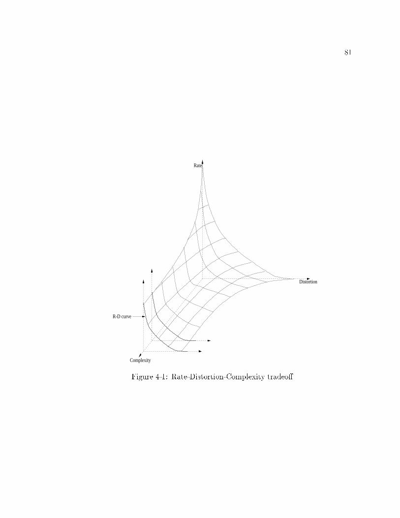
81

Distortion

Rate

Complexity

R-D curve

Figure 4-1: Rate-Distortion-Complexity tradeo�.

82

Unfortunately, the �niteness of an FSM is not a mathematically useful concept. The

�niteness constraints can often get in the way of a concise, understandable descrip-

tion of an algorithm. We often, for example, write programs in which we assume

that all our intermediate results will �t in their respective variables. Even though

the assumption may not always be strictly justi�ed, by making it, we greatly reduce

the amount of detail we have to handle and this is certainly desirable". From a

pure compression point of view, the FSM model is su�cient, under stationary and

ergodic assumptions. In this case, traditional compression algorithms (like Shannon-

Fano, Hu�man, or even universal extensions of arithmetic coding and Lempel-Ziv

coding) yields asymptotically optimal representations. This fact is clearly shown in

[70] where encoders and decoders are modeled by transducers which are FSM's with

a �nite amount of memory. But when the understanding problem is considered, the

content and the clarity of the descriptions become important factors that forces us to

extend the FSM model to the TM model with in�nite memory, as we commonly do

with real computers which are physically transducers with a large but �nite amount

of memory and time.

The deterministic framework provided by the Kolmogorov complexity allows the

de�nition of the RBCDF but it does not have the mathematical elegance of Shan-

non's probabilistic setting. Indeed, it is quite di�cult to make precise statements

on the properties of this complex rate-distortion-complexity relationship with the

tools that we have developed so far simply because we do not rely on a strong and

well known mathematical framework like probability theory. The most important

properties of the classical rate distortion function were derived from the connections

made with the mutual information. Similarly, we established connections with the

probabilistic setting and connect the RBCDF and mutual information by extending

the equivalences proposed in the previous chapter. The result of this is the following

83

theorem.

Theorem 1 Let [A;�] be a recursive stationary ergodic source. Let

P t;sD =

�� j � 2 P t;s

n ;Zdn(x

n1 ; y

n1 )dp � D

�(4.6)

where P t;sn is the class of probability measures for objects of length n, with cumulative

densities arithmetically computable in less than t steps and using less than s memory

cells. De�ne

Rn(D; t; s) = minPt;s

D

Inn

(4.7)

where In is the mutual information as it is de�ned in chapter 2 and

R(D; t; s) = limn!1

Rn(D; t; s) (4.8)

then,

limn!1

�C t;sD = R(D; t; s) (4.9)

for all t � Tmin and s � Smin, where

Tmin = infnt j P t;s

D 6= �o;

Smin = infns j P t;s

D 6= �o

� representing here the empty set.

Before we go on with the proof, note that Tmin and Smin are well de�ned simply

because of the existence of recursive coding procedures operating at any level D.

Also, by arithmetically computable in less than t steps and using less than s memory

cells, we simply mean that the cumulative density can be encoded by an arithmetic

coder using less than t steps and less than s memory cells.

84

Proof: This theorem is proved by using equivalences between information theory

and complexity distortion theory presented in chapter 3. Stationarity is assumed

here to make sure that the limit limn!1Inn

exists. To �nd this equivalent form,

recall the de�nition of P t;sD :

P t;sD =

�� j � 2 P t;s

n ;Zdn(x

n1 ; y

n1 )dp � D

�(4.10)

where P t;sn is the class of probability measures for objects of length n, with cumu-

lative densities arithmetically computable in less than t steps and using less than s

memory cells. Clearly, all probability measures belonging to P t;sn are recursive. Also

recall that:

Rn(D; t; s) = minPt;sD

Inn

(4.11)

Note that from the equivalence between CDT and RDT, for a stationary ergodic

source,

limn;t;s!1

Rn(D; t; s) = limn;t;s!1

�C t;sD (xn1) = lim

n!1CD(x

n1) �-a.s. (4.12)

We show that this equivalence still holds without the limits on computational re-

source bounds. To see this, consider the optimal conditional probability distribution

� 2 P t;sn that minimizes In. Let � be the induced probability distribution on the

reproduction space. It is easy to realize that

C t;s(yn1 ) � � log �(yn1 ) + c� (4.13)

since � is recursive and from a program computing �, we can represent yn1 with less

than t steps and less than s memory cells using the procedure used in arithmetic

coding. c� is just a constant independent of yn1 . Furthermore, from theorem 4,

85

chapter 3,

C(yn1 ) � C t;s(yn1 ) � � log �(yn1 ) + c� (4.14)

From theorem 8.1.1 in [52],

0 ��Z

C(yn1 )d� �H(�)�� c�0 (4.15)

where c� 0 is again a constant that does not depend on yn1 . As a consequence, if

we take expectations on equation 4.13, and we combine this with equation 4.15, we

obtain:

H(�) �ZC(yn1 )d� �

ZC t;s(yn1 )d� � H(�) + maxfc� ; c�0g (4.16)

As n grows to in�nity and dividing everything by n, we get:

limn!1

H(�)

n� lim inf

n!1

1

n

ZC t;s(yn1 )d� � lim sup

n!1

1

n

ZC t;s(yn1 )d� � lim

n!1

H(�) + maxfc�; c� 0g

n

(4.17)

Since the entropy rate converges for stationary sources, limn!11n

RC t;s(yn1 )d� exists

also and we conclude that

limn!1

H(�)

n= lim

n!1

1

n

ZC t;s(yn1 )d� (4.18)

Using randomness tests, we have also shown in the previous chapter that

limn!1

� log �(yn1 )

n= lim

n!1

C(yn1 )

nalmost surely

Since we assume � 2 P t;sn , it follows that

limn!1

� log �(yn1 )

n= lim

n!1

C t;s(yn1 )

nalmost surely

86

Hence,

limn!1

1

nQt;s

D (xn1) = limn!1

arg mindn(xn1 ;y

n1)�D

C t;s(yn1 ) = limn!1

arg mindn(xn1 ;y

n1)�D

� log �(yn1 ) almost surely

Clearly, Qt;sD de�nes then a channel mapping that minimizesR(D; t; s) almost surely

and corresponds to �. And using this deterministic channel mapping, limn!H(�)n

=

In = limn!11n

RC t;s(yn1 )d� and we get:

R(D; t; s) = limn!1

1

n

ZC t;s(yn1 )d� (4.19)

It remains to show that limn!11n

RC t;s(yn1 )d� = limn!1

�C t;sD . This is trivial since

yn1 = Qt;sD (xn1) and �(y

n1 ) =

PQt;s

D

�1(yn1)�xn1 , where Q

t;sD

�1(yn1 ) represents the set of all

sequences xn1 with image yn1 using Qt;sD (�). Hence,

limn!1

1

n

ZC t;s(yn1 )d� = lim

n!1

1

n

Xyn1

Xxn12Q

t;s

D

�1(yn1)

= limn!1

1

n

ZC t;s(yn1 )d�

and we have shown that

limn!1

�C t;sD = R(D; t; s) (4.20)

2

From this result, the most important property of this surface, convexity, can be

derived as stated in the next theorem:

Theorem 2 The average resource bounded complexity distortion function is convex

in the region where t � Tmin and s � Smin, where

Tmin = infnt j P t;s

D 6= �o;

87

and,

Smin = infns j P t;s

D 6= �o

Proof:

The convexity property is derived using theorem 1 and the properties of the mutual

information. First, note that the average distortion and the average complexity are

linear functions of the conditional distribution . To see this, choose two distinct

conditional distributions q1 and q2 operating at two distinct points on the average

resource bounded complexity distortion surface. At these points, let R1 and R2 be

the corresponding information rates. Let (�1;1) and (�2;2) be the corresponding

encoder/decoder pairs inducing q1 and q2. Let 0 � � � 1, then

D(�q1 + (1� �)q2) = �D(q1) + (1 � �)D(q2)

and, if (��;�) is de�ned as the encoding/decoding pair inducing the conditional

distribution �q1 + (1 � �)q2, then it is easy to realize that (��;�) operates at

a distortion level equal to D(�q1 + (1 � �)q2) and with average time and space

complexity given by:

T (�q1 + (1 � �)q2) = �T (q1) + (1� �)T (q2)

and

S(�q1 + (1 � �)q2) = �S(q1) + (1� �)S(q2)

From equation 4.20 the average resource bounded complexity distortion function can

be expressed as a mutual information which is a convex function of the conditional

distribution [15]. Denote R� the information rate at �q1 + (1 � �)q2. Then, R� �

�R1 + (1� �)R2, proving theorem 2.

88

2

Convexity is a key property to understand. It justi�es the usage of standard

optimization tools in order to design e�cient computational resource management

algorithms in such programmable environments. Note that the theorem holds with

a limit and also with stationary assumptions on the source. In general, convexity

is not true without this limit simply because the set of non random objects have

a non zero measure without this limit. But in general, Barron's lemma (that has

been further extended to the lossy case in [46]) provides an intuitive argument that

would guarantee convexity most of the time. Precise statements on this point still

remain to be established.

4.3. Universal Coding of Finite Objects with Distortion

and Computational Constraints

The convergence between complexity distortion function and rate distortion function

is due to the existence of types or relative frequencies. Classical coding techniques

use this property and are only asymptotically optimal for stationary ergodic sources.

The question that we address in this section is the design of e�cient codec systems

for �nite objects with a limited amount of computational resources. The goal is

to �nd a representation with performances as close as possible to the complexity

distortion function. To do so, we adopt a novel approach to universality that we

present in section 4.3.1. The problem becomes a mixture of Solomono�'s time

(resource) limited optimization problem and McCarthy's inversion problem. In the

time limited optimization problem, we have a machine M , whose inputs are �nite

strings and whose outputs are numbers. We are given a �xed time T 3. The problem

3More generally we are given a �xed amount of computational resources.

89

is to �nd within time T an input string, s, such thatM(s) is as large as possible. In

McCarthy's problem [55], we are given a partial function fm(n) computed by themth

TM4and we would like to design a TM which, when confronted by the number pair

(m; r), computes as e�ciently as possible a function g(m; r) such that fm(g(m; r)) =

r. Here, e�ciency hints towards computational resource bounds at the encoding

end. Clearly, g is not recursive, but following a construction identical to the one

used in the proof of theorem 4, chapter 3, we can approximate g. Unfortunately,

this procedure is highly ine�cient and not practical. Levin in [51] approached this

problem and proposed the LSEARCH (as it is called by Solomono� [77]) algorithm5.

This algorithm has been used and extended by Solomono� and Levin to include

time limited optimization problems. \The most general kind of induction can be

formulated as the problem of �nding short descriptions of data, which is a time

limited optimization problem, and therefore amenable to LSEARCH" [77]. To tackle

problems e�ciently, heuristics were added in the search to reduce the size of the

search space. The probabilistic analog of a heuristic is a function that assigns low

probabilities to areas of the search space that would be cut out by the heuristic. In

the machine learning theory this is called the\inductive bias". Furthermore it would

be necessary to have to machine modify the probability distribution over the search

space as a result of its own experience in problem solving. Evolutionary search

techniques provide us a natural way to achieve these goals. In section 4.3.3, we

focus on Genetic Programming. Following the novel approach to universal coding

(section 4.3.1), we proposed a coding system for �nite objects yielding performances

arbitrarily close to the resource bounded complexity distortion function. After a

4m is just the G}odel number or the index of this TM in a standard enumeration of TM's. See[52] for a discussion on standard enumeration of TM's.

5See [51], [52] chap 7, pp 503-505 for a good presentation of LSEARCH. A brief summary ofits extensions can be found in [77].

90

presentation of the decoding end of the communication system, we present the

encoder and provide an analysis of the time complexity of the proposed algorithm.

4.3.1 Universal Coding Revisited

Current universal coding techniques approach optimality asymptotically, as the

length of the observation increases to in�nity. By de�nition, a codec system is

universal if its coding rate approaches asymptotically the rate distortion function.

With stationary and ergodic assumptions, such systems have been designed and

categorized in three classes as discussed in chapter 2. E�orts to break the bar-

rier imposed by these non realistic statistical assumptions are presented in [22, 13],

with optimality still achieved asymptotically. Universal coding of �nite objects does

not �t naturally in this framework and in this section we address this problem by

showing how deterministic source models can also be used to model e�ciently �nite

objects. We believe that this extension is necessary in image processing simply be-

cause most natural images do not appear random or patternless to us because of the

structure and limitating capabilities of the HVS. Consequently, probabilistic models

should not be forced on such data just for tractability reasons. Deterministic models

should also be considered and the actual information content, which is irrelevant for

in�nite objects, should not be ignored. Under these lines, we formalize the universal

coding problem for �nite objects and add a fourth class into the taxonomy of lossy

universal coding techniques. For practical consideration, we restrict our attention

to recursive decoding functions and also consider decoding resource bounds in the

setting.

De�nition 1 Let the probability of error P (n)e be de�ned as follow:

P (n;te;se)e = �fxn1 j dn(x

n1 ;�

td;sdn (te;se

n (xn1))) � Dg (4.21)

91

We say that a rate R block code corresponding to the encoding/decoding pair (�n;n)

is algorithmically universal if the functions �n and n are recursive and if

limse;te!1

P (n;te;se)e = 0 (4.22)

whenever R � C td;sdD (xn1)

Theorem 1 For a �xed computational constraint (td; sd) and distortion constraint

D, algorithmically universal codes exist.

Proof:

With computational resource bounds at the decoding end, recursive encoders oper-

ating arbitrarily close to C td;sdD (xn1 ) do exist, proving the theorem.

2

In this setting, the decoder being a universal Turing machine, we also have a two

stage coding process, the �rst one describing an algorithm (or a TM) and the second

one describing the data for this algorithm (the program for that TM). The universal-

ity of this machine is precisely what we try to exploit to extend the classical notion

of universal coding and include all coding techniques, from traditional approach

like Hu�man, Arithmetic or even Lempel-Ziv techniques to modern approach like

model-based and fractal-based coding techniques. In fact, with the Church-Turing

thesis, we consider all representation techniques from an algorithmic angle and unify

them under the same framework. The general structure of this encoder is shown in

�gure 4-2. With such a universal decoder, what we are really doing here is allowing

more complex languages than the one used in traditional VQ systems, at the decod-

ing end. The design of such VQ decoders is a simple language design problem. The

\grammar" of such languages is very simple and it allows only one instruction, the

READ instruction that is used to access di�erent locations of the codebook. The

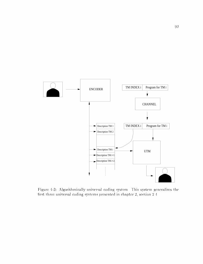
92

Description TM i+1

Description TM i+2

TM INDEX iENCODER

UTM

Program for TM i

Program for TM i

CHANNEL

Description TM 1

Description TM 2

Description TM i

TM INDEX i

Figure 4-2: Algorithmically universal coding system. This system generalizes the�rst three universal coding systems presented in chapter 2, section 2.4.

93

\vocabulary" of the language is contained in these codebooks. With a universal

Turing machine at the decoding end, we are allowing more complex grammars to

be used to represent the source data. Ideally, we would like to have a high level

language at the decoder that would help us to extend the traditional pixel oriented

way of representing visual information and reduce the gap between high level and

low level semantics of the source data. This language design step is equivalent to the

probability estimation step in classical IT. In practice, this design should depend

on the prior knowledge on the application at hand. This situation is similar to the

one we have to face when we design software systems. We would rather use LISP

than C for arti�cial intelligence applications, although both languages are Turing

complete. Similarly, there is an urgent need for a Turing complete language for

the representation of images. This problem is outside the scope of this thesis but

it is important to remember that good language design choices limit the software

overhead imposed by the �rst stage of the representation. In theory, this model

overhead becomes negligible for in�nite sequences but in practice, it must be taken

into account. Such a Turing complete language is used in MPEG-4 Audio. It is

called Structured Audio Orchestra Language [21].

4.3.2 The Decoder

The key component of the complexity distortion approach is the substitution of

the decoder in Shannon's classical communication system by a Turing machine. To

simplify the discussion, we assume that our decoding TM, n is a multitape TM with

a one way read only input tape called the program tape. Our input alphabet contains

four symbols: B = f0; 1; �; �g. � is the typical blank symbol. We add an extra

symbol � that will be used as a special character representing the \no operation"

instruction. This will greatly simplify the theoretical analysis of the convergence of

94

the algorithms. When the decoder scans this symbol on its program tape, it stays

in the same state and simply moves the program head one cell to the right. Its

meaning is equivalent to the use of introns and selector operators in biology and in

[53]. TM programs are isomorphically equivalent to LISP statements or symbolic

expressions. In fact compilers use this fact to translate any piece of code into their

equivalent abstract syntax tree representation. Introns6 refer to parts of a program

that do not a�ect its computation. Selector operators are simple function nodes in

abstract syntax trees that selects one and only one outgoing edge for traversal. This

way they link potential interesting parts of the programs in a non ambiguous way,

just like the � operation does on TM program strings. Designing the language of

the decoder delimits the space of possible representations that we call the program

search space. With a Turing complete language, optimal representations yielding

compression rates close to the complexity distortion function belongs to the search

space. Also, there is a constant c, such that for any x 2 A, C(xn1) � n + c [52].

Hence, by a trivial counting argument, we see that the problem of encoding xn1 can

be reduced to a search problem in a space containing 2n+c+1 � 1 programs if we

ignore introns.

4.3.3 The Encoder

With the program space speci�ed by the structure of the decoder, the encoder has

to explore this space and �nd an e�cient representation for the source object to

encode. The idea behind genetic programming is to perform a beam search which is

a compromise between exhaustive and hill climbing techniques[4]. In contrast with

genetic algorithms, programs are not restricted to have the same length. An evalu-

ation metric, commonly called a �tness measure, is used to measure the e�ciency

6The terminology is borrowed from biology where it is also referred as \junk DNA".

95

of each point in the program space. This number is a measure of how well the

corresponding program represents the source object. When lossy compression with

resource bounds at the decoder is the main problem, the �tness has to be a func-

tion of the amount of distortion introduced by the representation, the length of the

representation and its computational complexity. The �tness is used to select out a

certain number of the most promising solutions for further transformation. It allows

us to incorporate heuristics probabilistically in the search and give more weight to

short and accurate representations. The genetic programming method starts by

generating randomly an initial population of programs, also called a generation.

These programs are then run for less than t steps and using less than s memory

cells to determine their �tness. Using these �tness numbers for this population, and

following the Darwin principle of survival of the �ttest, a new generation of pro-

grams is obtained by performing genetic operations. The most common operations

are the crossover, the mutation and the reproduction. In the crossover operation,

two parent programs belonging to the initial generation are chosen. Subtrees of

these programs are randomly chosen and swap to give birth to two o�springs in the

new generation. The mutation operation simply changes randomly some nodes in

the abstract syntax trees of individuals of the new generation. The reproduction

copies good programs in the new generation. Details of these operations can be

found in [4]. What is interesting here is that under general conditions (to be men-

tioned below), when this process is repeated, the probability to have an element

with maximum �tness in the population converges to 1 [91]. To see this, note that

the dynamic of this algorithm can be modeled by a Markov chain. Populations have

�xed size, each possible one corresponding to a state in the Markov chain. Since

the object that has to be coded is �nite in length, the number of possible states in

96

this process is �nite7. The convergence of the genetic algorithms (with �xed length

representations) depends on the structure of the transition matrix Q of this Markov

chain. As shown in [91], optimality can be reached almost surely in polynomial time

if the following to points are satis�ed:

1. The second largest eigenvalue8 of Q, denoted ��, is suitably bounded away

from 1 so that the Markov chain is rapidly mixing.

2. The stationary distribution � gives probability greater than �, where 1�is poly-

nomial in the problem parameter, to the set of states that contains individuals

of best �tness.

The �rst property requires that Q is irreducible with non negative entries which

will always be the case if we have a strictly positive mutation probability forcing

ergodicity. The second property is more di�cult to satisfy. It can be ensured by

a good design of the decoder. Assuming that it also holds, the following algorithm

can be used at the encoder:

1. From a start state, evolve through a polynomial number of generations;

2. From the �nal population vector, select the �ttest individual.

3. Repeat step 1 and 2 a polynomial number of times.

The third step of the algorithm is necessary to boost the convergence probability.

Almost surely discovery of an individual with optimal �tness is guaranteed as long as

property 1 and 2 are veri�ed. Unfortunately, to our knowledge, it is still unknown

whether property 2 holds for GP systems where the representation length is not

7Formally, there is a constant c such that for all xn1 2 Bn

0 , C(xn

1 ) � n + c. Therefore, thecardinal of the program space is bounded.

8The largest eigenvalue of Q is 1 if the chain is irreducible. Its associated left eigenvector isthen �, the stationary distribution.

97

�xed. The problem comes from the variable length representation of GP which

prevents the derivation of closed form expression for the transition matrix.

4.4. Convergence Analysis of Genetic Programming

In contrast with GA, the behavior of GP is not well understood, and the theoretical

analysis of the GA model cannot be directly applied to GP. Fortunately, for problems

where an upper bound on the representation length is known, it is possible to modify

a GP search into a GA search. The idea here is taken from [53]. We stu� the symbol

� in programs in order to �x their length to the maximum n+ c. We then perform

a GA search on those extended strings before cleaning the optimal solution by

removing the introns �. Fix L = n+ c. ByM we denote the population size of each

generation. A program p is a string of length L, p 2 BL. From now on, by l(p),

we denote the length of the program p without the introns � that were arti�cially

introduced to �x the length of the program strings. Since B is �nite, we can de�ne

a lexicographic order on elements of BL and represent them with unsigned integers

identifying their place in the lexicographic list. We assume that the ordering is done

in the following manner:

1. All programs with outputs yielding strings inside the D-ball centered at xn1 are

ranked based on their length, the shortest ones having a lower lexicographic

index. These programs respect the distortion constraint D.

2. All programs with outputs yielding strings outside the D-ball centered at xn1

are ranked based on the amount of distortion they introduce when representing

xn1 .

3. All programs with outputs yielding strings inside the D-ball centered at xn1

have lexicographic index lower than any program yielding output strings out-

98

side the D-ball centered at xn1 .

From this convention, it is easy to see that the best individuals have very low

lexicographic indices. It remains to �nd an e�cient way to identify these indi-

viduals in polynomial time. This lexicographic order allows each population k to

be represented by a vector (Z(0; k); Z(1; k); � � � ; Z(�L � 1; k)) whose entries Z(i; k)

denotes the occurrences of individual i in population k, 0 � i � �L � 1, where9

� =j B j �1 = 3. . It is easy to see that the total number of di�erent population is

given by [60]:

N =

M + �L � 1

M

!(4.23)

Let f be the �tness function that assigns a real number to the lexicographic index

of each program. For a program p with index ip, f(ip) is a function of its length

and the amount of distortion introduced by the representation on the decoder n

after execution in less than t steps and using less than s memory cells. De�ne f as

follows:

f(ip) = 1(D(p) > D)Dmax + � �D(p)

Dmax + �

+ 1(D(p) � D)(n + c� l(p) + 1) (4.24)

where � is a strictly positive real number, c an integer constant such that 8xn,

C(xn1) � n + c. Dmax is an upper bound on the amount of distortion that can be

introduced at the encoder. Dmax = sup(xn1;yn1)2An�Anfdn(xn1 ; y

n1 )g. Finally, D(p) =

dn(xn1 ;(p)).

Lemma 1 The function f de�ned in equation 4.24 respects program ranks i.e. f is

monotonic decreasing on its domain.

9The blank symbol is not part of the representation. That's why � =j B j �1.

99

Proof of lemma 1: Let p1 and p2 be two elements of BL. Assume without loss

of generality that ip1 � ip2 then following the de�nition of the lexicographic order,

either of the following must be true:

1. D(p1) � D;D(p2) � D and l(p1) < l(p2)

2. D(p1) > D;D(p2) > D and D(p1) � D(p2)

3. D(p1) � D and D(p2) > D

Case 1: Since D(p1) � D and D(p2) � D,

f(ip1) = n+ c� l(p1) + 1

and

f(ip2) = n+ c� l(p2) + 1

Since l(p1) � l(p2), f(p1) � f(p2). Hence, the lemma holds for case 1.

Case 2: Since D(p1) > D and D(p2) > D,

f(ip1) =Dmax + � �D(p1)

Dmax + �

f(ip2) =Dmax + � �D(p2)

Dmax + �

Since D(p1) � D(p2), f(ip1) � f(ip2). Hence, the lemma holds for case 2.

Case 3: Since D(p1) � D and D(p2) > D,

f(ip1) = n + c� l(p1) + 1 � 1 � f(ip2) =Dmax + � �D(p2)

Dmax + �

. Hence, f(ip1) � f(ip2) and the lemma holds for case 3.

The lemma is proved.

100

2

Note that when the distortion is smaller than the constraint D, the �tness cri-

terion takes into account only the length of the representation. In practice, this

should not matter as long as the distortion constraint is not violated.

The GA search is identical to the GP search. It starts with a random generation

of M di�erent programs constituting the �rst generation. Then, the following three

steps are used to generate new good programs:

1. Selection: Compute the following probabilities:

p(i; k) =f(i)Z(i; k)P�L�1

h=0 f(h)Z(h; k)(4.25)

p(i; k) is just the probability of having program i at generation k. With these

probabilities, randomly select two programs.

2. Crossover: Generate two new individuals by exchanging the 1 � l � L � 1

right most symbols of the two individuals obtained by the selection phase.

The number of exchanged symbols l is chosen uniformly at random10, from

[1; L� 1].

3. Mutation: Invert, with probability � the actual bits (symbols equal to 0 or

1) in the program of the two new individuals obtained from the crossover

generation. Ignore the introns.

A new generation is then obtained by reserving the M � 2m;m 2 f0; 1; � � � ;M=2g

programs with the highest �tness in the previous generation and applying the three

genetic steps, selection/crossover/mutation, to get � = 2m new individuals. Clearly,

this process can be modeled by a Markov chain with state space S corresponding

10To simplify the discussion, we consider here the one-point crossover.

101

to the set of all N di�erent generations. Consider a lexicographic ordering of these

N generations; the N � N transition matrix Q = (Qk;v) of this process has been

computed by Vose et al. in [60]. Qk;v is just the conditional probability to move to

generation v from generation k. When the number of generated individuals equals

exactly � = 2m =M , M even, it is shown in [60] that:

Qk;v =M !�L�1Yj=0

1

Z(j; v)!r(j; k)Z(j;v) (4.26)

where r(j; k) is the probability that individual j occurs in population k. This can be

proved by noting that Z(j; k) is generated according to the multinomial distribution

based on r(j; k); j = 0; 1; � � � ; �L� 1;. See [60] for a derivation of r(j; k) for a binary

alphabet.

4.4.1 Convergence

Let q(0) = (q(0)1 ; q(0)2 ; � � � ; q(0)N ) be the initial distribution of the Markov chain. The

distribution at generation n is given by q(n) = (q(n)1 ; q

(n)2 ; � � � ; q(n)N ) = q(0)Qn, Qn

being the n-th power of the transition matrixQ. The objective of the algorithm is to

converge as fast as possible to a population that includes an optimal program. Let �

be the set of populations which include the individual with the highest �tness value.

In this section, we investigate how closelyP

k2� q1k is to one. In [67], it is shown that

the transition matrix of the simple GA with � = 2m = M is primitive (irreducible

aperiodic) and this implies thatP

k2� q1k does not converge to one since the other

states k =2 � are also recurrent non null. It does converge to a stationary distribution

and Monte Carlo sampling can be used to almost surely discover the best individual

[91]. In [85], almost surely convergence is obtained in another fashion by preventing

the genetic operators from reducing the performance of the best individual during

the evolution. In that paper, a spot is always reserved in the next generation for the

102

best individual of the current generation. In this modi�ed GA algorithm, also called

the elitist strategy, � is set at 2m = M � 1, M obviously odd. As a consequence,

the transition matrix becomes:

Qk;v = (M � 1)!�L�1Yj=0

1

Y (j; v)!r(j; k)Y (j;v) (4.27)

for i�(k) � i�(v), and 0 for i�(k) < i�(v), where i�(j) is the index of the best program

in generation j, and where

Y (j; k) =

8><>:

Z(j; k) if j 6= i�(k)

Z(j; k)� 1 if j = i�(k)

In this case, the transition matrix Q is indecomposable (reducible with only one

aperiodic recurrent class). In fact, it is shown in [85] that Q has �L sub-matrices

Q(i) of size N(i) � N(i), i = 0; 1; � � � ; �L � 1, as diagonal elements and all the

components to the upper right of these sub-matrices are zeros. N(i) is the number

of populations k in which i = i�(k). It is shown to be:

N(i) =

M � 1 + �L � i

M � 1

!(4.28)

It is shown in [85] that for this modi�ed GA algorithm, there is a constant C such

that Xk2�

q(n)k � 1� C j �� j

n; (4.29)

where

j �� j= max1�i�2L�1

max1�j�N(s)

j �i;j j (4.30)

and �i;j , j = 1; 2; � � � ; N(i) denotes the N(i) eigenvalues of the sub-matrix Q(i),

i = 0; 1; � � � ; 2L � 1 which are identical to the eigenvalues of Q. Since �� is less

103

than 1, convergence is guaranteed. The convergence to one can also be guaranteed

by decreasing gradually the mutation probability in a simulated annealing fashion.

In fact, the analogy with simulated annealing can be taken further. The mutation

operator can be interpreted as a temperature parameter controlling the stability

of the system. It also guarantees convergence in the almost sure sense to globally

optimal solutions. With a proper \cool down" schedule [29, 86, 84], convergence is

guaranteed [29, 86].

All these results prove the existence of a family of probabilistic algorithms con-

verging to the best individual with probability 1. Note that this convergence to 1

although necessary, is not su�cient for the design of an e�cient coding system. Af-

ter all, if this was the only criterion for e�ciency, we would have used a full search

method. This is precisely why we analyze the speed of the convergence of these

techniques in the next section.

4.4.2 Speed of Convergence

Ideally, we would like to reach any reasonable level of convergence (in terms of

probability to �nd optimal representation) in polynomial time with a reasonable

polynomial exponent. To formalize this, we follow the concept of rapidly mixing

Markov Chain as described in [75].

De�nition 1 Consider a family of Markov ChainsMC(x) parameterized on strings

x 2 A, with a �nite set of states S, transition matrix Q = (Qij), stationary dis-

tribution (when it exists) � = (�i) and relative pointwise distance (r.p.d.) for each

x 2 A, over U � S after t steps,

�(x)U (t) = max

i2S;j2U

j Q(t)ij � �j j

�j

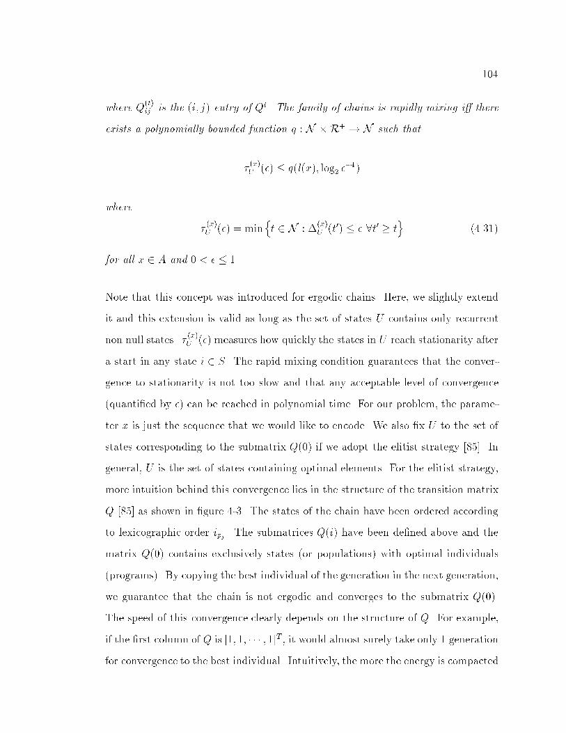
104

where Q(t)ij is the (i; j) entry of Qt. The family of chains is rapidly mixing i� there

exists a polynomially bounded function q : N �R+ !N such that

�(x)U (�) � q(l(x); log2 �

�1)

where

�(x)U (�) = min

nt 2 N : �(x)

U (t0) � � 8t0 � to

(4.31)

for all x 2 A and 0 < � � 1.

Note that this concept was introduced for ergodic chains. Here, we slightly extend

it and this extension is valid as long as the set of states U contains only recurrent

non null states. � (x)U (�) measures how quickly the states in U reach stationarity after

a start in any state i 2 S. The rapid mixing condition guarantees that the conver-

gence to stationarity is not too slow and that any acceptable level of convergence

(quanti�ed by �) can be reached in polynomial time. For our problem, the parame-

ter x is just the sequence that we would like to encode. We also �x U to the set of

states corresponding to the submatrix Q(0) if we adopt the elitist strategy [85]. In

general, U is the set of states containing optimal elements. For the elitist strategy,

more intuition behind this convergence lies in the structure of the transition matrix

Q [85] as shown in �gure 4-3. The states of the chain have been ordered according

to lexicographic order ipj. The submatrices Q(i) have been de�ned above and the

matrix Q(0) contains exclusively states (or populations) with optimal individuals

(programs). By copying the best individual of the generation in the next generation,

we guarantee that the chain is not ergodic and converges to the submatrix Q(0).

The speed of this convergence clearly depends on the structure of Q. For example,

if the �rst column of Q is [1; 1; � � � ; 1]T , it would almost surely take only 1 generation

for convergence to the best individual. Intuitively, the more the energy is compacted

105

in the lower diagonal of Q, the faster the process will converge. The second largest

eigenvalue �� of Q dictates the speed at which the process converges to optimality.

Clearly, the lower j �� j is, the faster the convergence is. Recall also from elemen-

tary algebra Gerschgorin's theorem that states that the module of each eigenvalue

of Q is upper-bounded by maxkP

v Qk;v. This theorem also applies to each of the

Q(i) submatrices, especially to the one having �� for eigenvalue. As a result, we see

that the magnitude of this eigenvalue is upper bounded by the amount of energy

in the most \energetic" row of one of the Q(i)'s. Note that transitions within the

submatrices Q(i) are not desired because these transitions corresponds to events

where the new generation does not discover anything new. The �tness of the best

individual does not increase in these cases. The magnitude of the second largest

eigenvalue is a very good indicator of the probability of having such transitions, as

being upper bounded by the maximum probability of not evolving. The larger this

value is, the slower the convergence is since most of the energy in Q will then be

in the submatrices Q(i) and not below the diagonal that these submatrices form.

These intuitive observations have a lot in common with the concept of conductance

discussed in [75] and can be generalized for the other genetic algorithms approaches.

In the rest of this section, we compute an upper bound for the r.p.d. of each chain

in the family de�ned by the encoding algorithm. Following the algebraic approach

proposed in [75], we derive general conditions on the second largest eigenvalue of Q

to guarantee the rapidly mixing property and show that it is possible to solve our

universal coding problem in polynomial time.

To ensure the rapidly mixing property, the following result is used: As mentioned

in [75], this de�nition of rapid mixing \is rather a strict one because it is based on

the relative pointwise distance, which is a severe measure for two reasons. Firstly,

it demands that the distribution of the chain be close to the stationary distribution

106

Q(0)

Q(1)

L

0Q

N(i)

N(i)

Q( α− 1)

Q(i)

Figure 4-3: The transition matrix for the elitist strategy.

at every point (in U for our problem) and secondly, it demands that convergence be

rapid from every initial state".

Lemma 2

�(x)U (t) �

j �t� j

minj2U �j

For all t even,

�(x)U (t) � �t�

Moreover, if all eigenvalues of P are non-negative, the lower bound holds for all

t 2 N

Proof: See [75]

2

Despite imposing restrictions in lemma 2, the sign of the eigenvalues never present an

obstacle to rapid mixing because any chain can be modi�ed to have all eigenvalues

positive, as explained in [75]. Hence, from this lemma, it is clear that the rapid

107

mixing property will be respected if and only if the second largest eigenvalue is

suitably bounded away from 1. We sum up this fact in the following theorem:

Theorem 3 The rapid mixing condition is guaranteed if and only if

1

log21j��j

= p(l(x); ; log2 ��1) (4.32)

p(l(x); log2 ��1) being a positive polynomial function in l(x), the size of the input.

Proof: Assume that the chain is rapid mixing. Then by de�nition, for each

0 < � < 1, there is a polynomially bounded function q : N �R+ ! N such that:

�(x)U (�) � q(l(x); log2 �

�1)

where

�(x)U (�) = min

nt 2 N : �(x)

U (t0) � � 8t0 � to

(4.33)

Hence,

8t � �(x)U (�);�

(x)U (t) � �

By lemma 2,

j �� jt� �

(x)U (t) � �

This implies that:

t log2 j �� j� log2 �

And this can be rewritten as:

t log21

j �� j� log2 �

�1

108

Therefore,

log2 ��1

log21j��j

� t;8t� �(x)U (�)

Since � (x)U (�) � q(l(x); log2 ��1), we conclude that

log2 ��1

log21j��j

= p(l(x); log2 ��1)

with l(x) = n + c for the universal coding problem.

Assume that

1

log21j��j

= p(l(x); log2 ��1)

From the de�nition of � (x)U (�),

8t � �(x)U (�);�(x)

U (t) � �

By lemma 2, if j��jt

�min� � then �(x)

U (t) � � where �min = minj2U �j. Saying that

j��jt

�min� � is equivalent to say that

t log2 j �� j� log2 �min�

and this can be rewritten as:

t �log2(�min�)�1

1j��j

The last equation holds for all t � �(x)U (�). Therefore, if log2(�min�)�1

1

j��j

is polynomial

in l(x) and log2 ��1, so is �

(x)U (�) and the chain is rapid mixing. And this will hold

if log2 ��1min is polynomial in l(x), a result that can be easily derived for the genetic

problem by taking a closer look at the mutation operator. In this case, note that

109

there is at least a probability equal to �L; (L = n + c) to change from any state of

the chain to any other state. Therefore, �min � �L and log21

�min� L log2

1�. We

conclude that the chain is rapid mixing and we have proved theorem 3.

2

In general, closed form expressions for �� are di�cult to compute but for one

point crossover systems it is shown in [97] that �(x)U (�) � l(x) ln(l(x)) + ln ��1. This

provides a bound for j �� j and shows that the proposed universal coding algorithm

is fast.

4.5. Algorithmic Representation of Images

In this section, we apply the algorithm described in the previous section to still

image data. Our aim is to model visual information deterministically, with no

probabilistic assumption. Similar experiments were performed by Nordin [61] on

images and sound and Koza [47] on images with primitive language that looked like

machine code with no theoretical analysis and little success in terms of distortion.

We take these experiments on step further and signi�cantly improve the quality

of the representation to approach acceptable levels in terms of distortion and rate,

despite using a very simple language also. We �rst describe the decoding operations

before presenting the encoding steps with a few experimental results.

4.5.1 The Decoder

The decoding device is completely speci�ed by its language. Tables 4.1 and 4.2

show a complete description of the instruction used for these tests. As shown there,

the language used is block-based. We restrict ourselves to blocks to keep the imple-

mentation simple. This language contains two types of functions and terminals, a

block type (blk) and an integer type (int). Function nodes involving the blk type

110

Instruction Return Type Argument 1 Argument 2 Argument 3 Action

Rotate blk (blk) block (int) angle { RotationScale blk (blk) block (int) angle { ScalingTFilt blk (blk) block (int) angle { FilterLFilt blk (blk) block (int) angle { FilterMin blk (blk) block (blk) input-block-2 { MinimizationMax blk (blk) block (blk) input-block-2 { MaximizationTrans blk (blk) block (int) arg1 (int) arg2 TranslationRead blk (int) x-index (int) y-index { Memory ReadWrite blk (int) x-index (int) y-index (blk) block Memory Write* int (int) arg1 (int) arg2 { Multiplication/ int (int) arg1 (int) arg2 { Division+ int (int) arg1 (int) arg2 { Addition- int (int) arg1 (int) arg2 { Subtraction

Table 4.1: Functions used to represent gray level image data.

generally perform spatial operations (rotations, scale, translation etc) except for

the Read and Write function nodes. These two functions are used to access a two

dimensional memory where blocks of data can be stored and retrieved during the

computation. There are also 2 terminal nodes of type blk that can used in the

computation. Most of the function nodes of type blk require integer parameter to

control their execution. The standard arithmetic operations +;�; �; = are used for

this purpose, together with integer terminals from 1 to 9.

This language is extremely simple. It is not even Turing complete but it contains

enough nodes to illustrate how the genetic programming approach described in the

previous section can be used to developed deterministic models for images. As

a result, we do not attempt to compete with state of the art image compression

systems [59, 68]. For this, we would need a much more complex language developed

from all the expertise that the image processing community has gained over the

years as discussed in chapter 5, section 5.2.2.

111

Instruction Return Type Action

Dark blk Terminal (blk)Light blk Terminal (blk)1 int Terminal (int)2 int Terminal (int)3 int Terminal (int)4 int Terminal (int)5 int Terminal (int)6 int Terminal (int)7 int Terminal (int)8 int Terminal (int)9 int Terminal (int)

Table 4.2: Terminals used to represent gray level image data.

4.5.2 The Encoder

The general encoder architecture is shown in �gure 4-4. At the heart of this system

is the GP module performing a GP search in the program search space de�ned by

the decoding language and working in tandem with the UTM. The GP module uses

the genetic operations described in section 4.3.3. To do so, we have developed a

Typed GP kernel that allows us to specify decoding programs with di�erent node

types. This system is an extension of the public GP system described in [27] which

like most GP kernel does not allow the use of nodes with di�erent return types in

the syntax of the decoding language.

Every time an incoming block is given to this module, a best program for the

representation of this block is found and tested. The resulting block is then stored

in the 2D memory and is now available for GP encoding of the future blocks. As

explained in �gure 4-5, the 2D memory is indexed from the location of the current

block to encoded in the following manner: assume that we would like to encode block

(x; y), x representing the column location in the image and y the row location. Then

memory indices (0; 0) would correspond exactly to position (x; y). Memory indices

(i; j) would correspond to absolute locations (x� i; y� j) in the memory. This way,

112

������

������

������

������GP

Learning Unit

UTM

2D Indexed MemoryInput Image

DCT VLC Selector

IDCTDeQuantQuant

Figure 4-4: Hybrid Image Encoder.

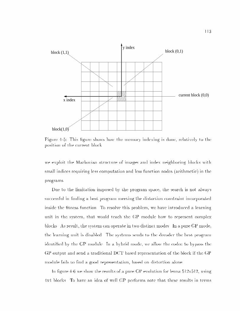
113

����������������������������

����������������������������

current block (0,0)x index

block(1,0)

block (1,1)y index

block (0,1)

Figure 4-5: This �gure shows how the memory indexing is done, relatively to theposition of the current block.

we exploit the Markovian structure of images and index neighboring blocks with

small indices requiring less computation and less function nodes (arithmetic) in the

programs.

Due to the limitation imposed by the program space, the search is not always

successful in �nding a best program meeting the distortion constraint incorporated

inside the �tness function. To resolve this problem, we have introduced a learning

unit in the system, that would teach the GP module how to represent complex

blocks. As result, the system can operate in two distinct modes. In a pure GP mode,

the learning unit is disabled. The systems sends to the decoder the best program

identi�ed by the GP module. In a hybrid mode, we allow the codec to bypass the

GP output and send a traditional DCT based representation of the block if the GP

module fails to �nd a good representation, based on distortion alone.

In �gure 4-6 we show the results of a pure GP evolution for lenna 512x512, using

4x4 blocks. To have an idea of well GP performs note that these results in terms

114

(a) (b)

Figure 4-6: Programmatic representation of lenna 512x512, psnr = 29.72 dB at 1.17bpp: (a) original, (b) gp output. In this run the language uses 4x4 blocks. Notethe large errors introduced in the top of the picture because of the inability of thelanguage to represent these blocks when the memory of the system is empty.

115

of psnr and number of bits per pixel (bpp) of the pure GP mode are still far from

what a DCT codec system would give using 8x8 blocks but this is mainly due to

the di�erence in block sizes and the limitations of the decoding language.

(a) (b)

Figure 4-7: This �gure compares 8x8 blocks with a signi�cant amount of edges (ac-cording to a Sobel edge detector) with blocks that cannot be represented accuratelyby the GP module. Edge blocks and GP blocks with large MSE are in white: (a)edge blocks, (b) GP blocks with large error. Note the similarities between this twopictures showing that the language did not manage to represent accurately most ofthe edge blocks.

Like VQ techniques, this pure GP systems does not perform well for blocks

bigger than 4x4 without help from the DCT learning unit. This is mainly due

to the use of the mean square error (MSE) in the �tness function as a distortion

measure. It is well known [30] that the MSE does a poor averaging job in VQ

type systems especially around the sharp edges of the image. These edges become

blurred. In �gure 4-7, we illustrate this point by showing the locations of the blocks

that could not be represented accurately by a pure GP system using 8x8 blocks.

These locations corresponds to the edges of the source images. With the learning

116

unit, the gp system performs closer to a standard DCT systems with variable length

coding. Experimental results are shown in �gures 4-8,4-9 and 4-10. In all cases, the

system was not able to encode the strong edges.

(a) (b)

Figure 4-8: Programmatic representation of lenna 512x512 with the learning unit,psnr = 32.97 dB at 0.9 bpp: (a) original, (b) gp output. In this run the language uses8x8 blocks. The learning unit introduced 1381 DCT blocks (out of 4096), mainly atthe strong edges of the image.

4.6. Conclusion

In this chapter, we have introduced computational resource constraints to source

coding. The result is an extension of the rate distortion function into a surface show-

ing the tradeo� between information rate, distortion and computational complexity,

that we called the complexity distortion surface. The convexity of this surface has

been established in the �rst part of this chapter by exploiting equivalences between

complexity distortion functions and mutual information. In the second part of the

chapter, we proposed a novel approach to universal data compression with an algo-

rithm able to perform at rates arbitrarily close to the complexity distortion surface.

We studied the converging properties of the proposed method before illustrating it

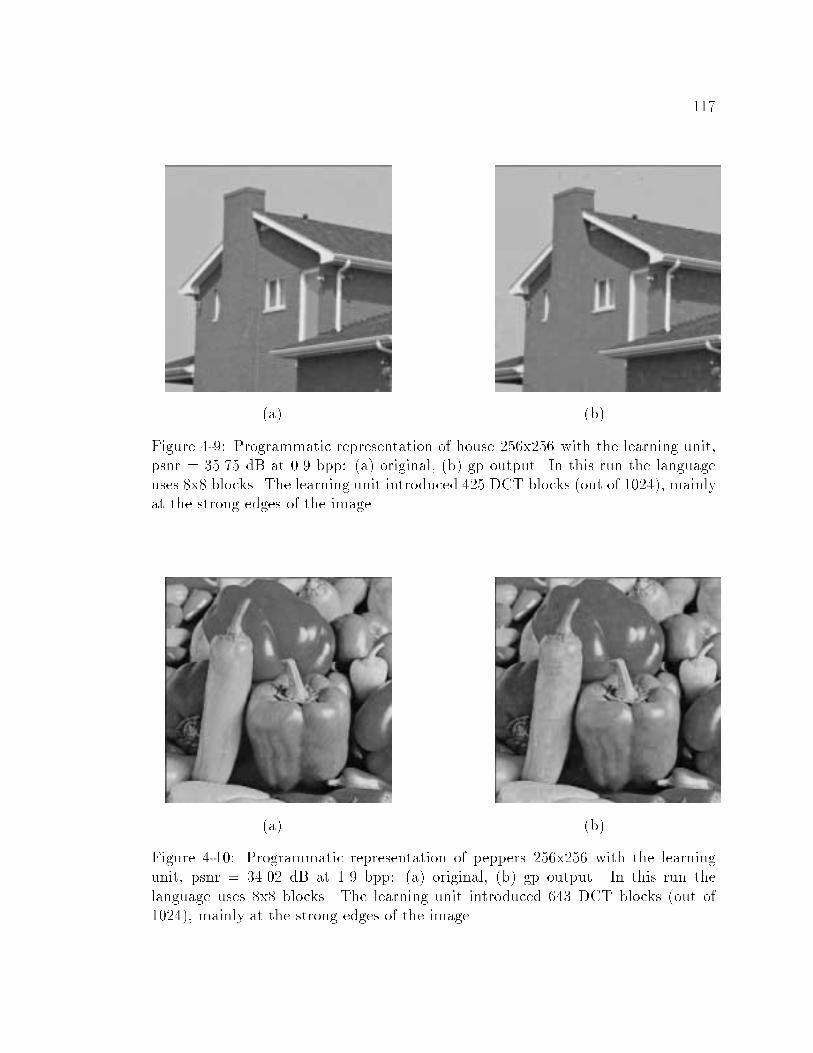
117

(a) (b)

Figure 4-9: Programmatic representation of house 256x256 with the learning unit,psnr = 35.75 dB at 0.9 bpp: (a) original, (b) gp output. In this run the languageuses 8x8 blocks. The learning unit introduced 425 DCT blocks (out of 1024), mainlyat the strong edges of the image

(a) (b)

Figure 4-10: Programmatic representation of peppers 256x256 with the learningunit, psnr = 34.02 dB at 1.9 bpp: (a) original, (b) gp output. In this run thelanguage uses 8x8 blocks. The learning unit introduced 643 DCT blocks (out of1024), mainly at the strong edges of the image

118

on gray level still image data. The proposed technique does not rely on any proba-

bilistic assumptions and does not require in�nite source objects for convergence to

optimality.

119

Chapter 5

Conclusion and future directions

5.1. Conclusion

We have presented a novel approach to source coding by extending Kolmogorov

complexity theory, which replaces the decoder by a universal Turing machine in

Shannon's classical communication system, to the lossy case yielding complexity

distortion theory. The motivation behind this work was initially behind the current

trend in media representation that requires a uni�ed approach for all the spec-

trum of coding techniques, from traditional entropy coding to modern approaches

like fractal and model-based coding. This current trend also sees the emergence

of new problems generalizing the classical compression rate/distortion optimization

into more complex problems which requires a better understanding of the informa-

tion content, i.e., object-based design, seamless access to content, editing in the

compressed domain, scalability and graceful degradation for network transmission,

graceful degradation with diminishing decoder capabilities, exibility in algorithm

selection, and even downloadability of new algorithms. With this in mind, we have

de�ned the complexity distortion function and proved that this function is equal

with probability one, to the rate distortion function for all stationary and ergodic

process with recursive probability measure. The mathematical derivation of this

120

equivalence is at the heart of this thesis. It clearly highlights two major points

of fundamental importance for the design requirements of today's communication

systems.

First, this result serves as theoretical bridge from Kolmogorov's deterministic

setting to Shannon's probabilistic setting enabling us to tackle very important issues

that are beyond the scope of traditional source coding, namely how to introduce

decoding computational resource considerations in information theory. These issues

can be de�ned clearly in Complexity Distortion Theory and then bridged to classical

information theoretic entities to bene�t from the well understood properties of the

main information theoretic concepts. Following this approach, we have de�ned the

tradeo� between computational complexity, information rate and distortion and

via links to the mutual information, we derived conditions for the convexity of this

surface, a key property for the design of e�cient resource management algorithms at

the decoding end of such programmable communication systems. This introduction

of resource bounds considerations also brings up several interesting open problems

related to our understanding of the capacity of a channel. These issues are discussed

next in section 5.2.1.

Second, the proposed proof for the equivalence between CDF and RDF identi�es

clearly the null set where these two entities are not equivalent. This set corresponds

to the set of non random sequences with strong deterministic patterns. Because

of its low measure, this set is neglected in the design of e�cient representation

algorithms. Typical algorithms like Lempel-Ziv, Hu�man Coding and Arithmetic

Coding ignore completely this set and focus on its much larger complement. This

complement does not have measure one for the coding of �nite objects but Barron's

lemma and randomness tests clearly show that it has a very high measure even for

�nite sequences. Hence from a mathematical perspective, this set does not seem to

121

have a signi�cant importance. Problems arise when we observe audio-visual (syn-

thetic and natural) objects around us and how they are perceived byt the human

visual system. They do have a lot of important structural properties that seems to

escape from our classical mathematical model. We believe that these objects have

strong components that belongs to this very small set of non random sequences.

Assuming the contrary would assume that these signals are completely patternless

and would prevent us from analyzing them with our human visual system. Moti-

vated by these observations, we have developed a novel approach to lossy universal

source coding for �nite length objects attempting to encode objects at rate closed

to the complexity distortion surface. Under these lines, we have proposed an ef-

�cient universal coding technique based on genetic programming. The technique

was then illustrated on image data, using a simple block-based language. These

simple experiments highlight the importance of designing good languages for media

representation as discussed in the following, in section 5.2.2.

5.2. Future directions

5.2.1 Channel Capacity versus System Capacity

Source coding with resource bounds brings up several interesting open questions

that have not receive much attention in information theory. Indeed, as mentioned

in [69], traditional information theory does not di�erentiate the channel capacity

from the system capacity. The former de�nes the maximum amount of information

that can be transmitted by a channel de�ned probabilistically with a conditional

distribution. The latter de�nes the maximum amount of information that can be

reproduced at the decoding end of the communication system. Clearly, with no

decoding computational constraints, these two quantities are equal since the only

bottleneck in the entire system is due to the reliability of the channel. With lim-

122

DECODING POWER

BITS PER SYMBOL

CHANNEL CAPACITY

SYSTEM CAPACITY

Figure 5-1: Channel and system capacities.

itations on the decoding power, these two concepts diverge. In fact, the channel

capacity is always larger than the system capacity simply because the channel is

part of the system. As the computational power of the decoder increases, the sys-

tem capacity gets closer and closer to the channel capacity (see �gure 5-1) and there

is an urgent need to understand this convergence. De�ning such a system capacity

is not natural in the classical IT framework. Once more, CDT provides an inter-

esting setting where this issue can be addressed. To do this, we could conceptually

group together the channel and both the source and channel decoder1, as shown in

�gure 5-2. We call the resulting block the system channel. We allow the decoding

operations to be lossy in order to meet the space and time requirements and the

system capacity takes into account this decoding loss of information. This situa-

tion is common in practice when a decoding general purpose digital signal processor

(DSP) has to meet various hard timing constraints imposed by the application and

1We group both the source and channel decoder together because computational bounds on thesource and channel decoder also a�ect the system capacity.

123

SOURCE ENCODER CHANNEL DECODER DESTINATION

SYSTEM CHANNEL

Figure 5-2: General system channel.

must drop signi�cant information to respect these constraints. More work on this

issue will be done in the future.

5.2.2 Language Design

E�cient representation languages for visual representation have yet to be formalized

in media representation. In audio processing, MPEG-4 introduced a Turing com-

plete language called Structured Audio Orchestra Language (SAOL). Under the

same lines, there is a need for the equivalent in image/video processing to improve

current state of art representation techniques beyond compression considerations.

Such a language should bene�t from the prior work in this �eld on which a sig-

ni�cant amount of new features could be added for Turing completeness and true

universality. We believe that this step is necessary for the design of visual informa-

tion system at high semantic levels. Currently, there is a signi�cant gap between

low level data at the bit level and high level data like it is perceived by the human

visual systems. A good representation language would signi�cantly close this gap

and enable the design of more powerful visual information systems. There is an

interesting analogy with general computing systems that also process information.

At the bit or even assembly language level, we can only dream about designing

complex applications like word processors or web browsers. With the development

of modern operating systems and modern computer languages like C/C++, these

dreams became reality. This addition of software layers on top of the raw hardware

124

enabled us to communicate in a more adequate way with the hardware. Similarly,

good representation languages would allow us to have better connections between

the human visual system and digital image/video data.

125

References

[1] E. Allender. Time Bounded Kolmogorov Complexity in Complexity Theory in

the Book Kolmogorov Complexity and Computational Complexity, chapter 2.Springer-Verlag, 1992.

[2] M. Anthony and N. Biggs. Computational Learning Theory, An Introduction.Cambridge University Press, 1992.

[3] O. Avaro, P. Chou, A. Eleftheriadis, C. Herpel, and C. Reader. The MPEG-4System and Description Languages: A Way Ahead in Audio Visual Informa-tion Representation. Signal Processing: Image Communication, 1997.

[4] W. Banzhaf, P. Nordin, R.E. Keller, and F.D. Fracone. Genetic Programming:

An Introduction. Morgan Kaufmann, 1998.

[5] M.F. Barnsley. Fractals Everywhere 2nd ed. Academic Press Professional,1993.

[6] T. Berger. Rate Distortion Theory: A Mathematical Basis for Data Compres-sion. Prentice-Hall, Inc., 1971.

[7] T. Berger and J.D. Gibson. Lossy source coding. IEEE Transactions onInformation Theory, 44.

[8] R.V. Book. On Sets with Small Information Content in the book KolmogorovComplexity and Computational Complexity, chapter 3. Springer-Verlag, 1992.

[9] C. Calude. Theories of Computational Complexity. North-Holland, 1988.

[10] C. Calude. Information and Randomness An Algorithmic Perspective.

Springer-Verlag, 1994.

[11] G. J. Chaitin. On the Length of Programs for Computing Finite Binary

Sequences. Journal of The Association for Computing Machinery, 13, 1966.

[12] G.J. Chaitin. A Theory of Program Size Formally Identical to InformationTheory. Journal of The Association for Computing Machinery, 22, 1975.

126

[13] P.A. Chou, M. E�ros, and R.M. Gray. A Vector Quantization Approach to

Universal Noiseless Coding and Quantization. IEEE Transactions on Infor-mation Theory, 42, 1996.

[14] T.H. Cormen, C.E. Leiserson, and R.L. Rivest. Introduction to Algorithms.McGraw-Hill, 1995.

[15] T. Cover and J. Thomas. Elements of Information Theory. John Wiley and

Son, 1991.

[16] I. Csiszar. The method of types. IEEE Transactions on Information Theory,44.

[17] M. Davis. Computability and Unsolvability. Dover Publications, Inc, New

York, 1982.

[18] L.D Davisson, G. Longo, and A. Sgarro. The Error Exponent for the NoiselessEncoding of Finite Ergodic Markov Sources. IEEE Trans. Info. Th., 27, 1981.

[19] D.L. Donoho, M. Vetterli, R.A. DeVore, and I. Daubechies. Data compressionand harmonic analysis. IEEE Transactions on Information Theory, 44.

[20] G.F. Luger ed. Computation and Intelligence. The MIT Press, 1995.

[21] R. Vaananen E.D. Scheirer and J. Huopaniemi. AudioBIFS: Describing AudioScenes with MPEG-4 Multimedia Standard. IEEE Transactions on Multime-dia, 1:3:237{250, 1999.

[22] M. E�ros, P.A. Chou, and R.M. Gray. Weighted Universal Image Compres-

sion. IEEE Transactions on Image Processing, 10, 1999.

[23] A. Eleftheriadis. Flavor: A Language for Media Representation. In Proceed-ings, ACM Multimedia 97 Conference, Seattle, WA, 1997.

[24] Y. Fang and A. Eleftheriadis. A Syntactic Framework for Bitstream-Level

Representation of Audio-Visual Objects. In Proceedings, 3rd IEEE Int'l Conf.on Image Processing, pages II.421{II.424, Lausanne, Switzerland, September1996.

[25] W. Feller. An Introduction to Probability Theory and its Applications, vol-ume 2. John Wiley & Sons, 2nd edition, 1957.

[26] G. B. Folland. Real Analysis, Modern Techniques and their Applications. JohnWiley & Sons, Inc, 1984.

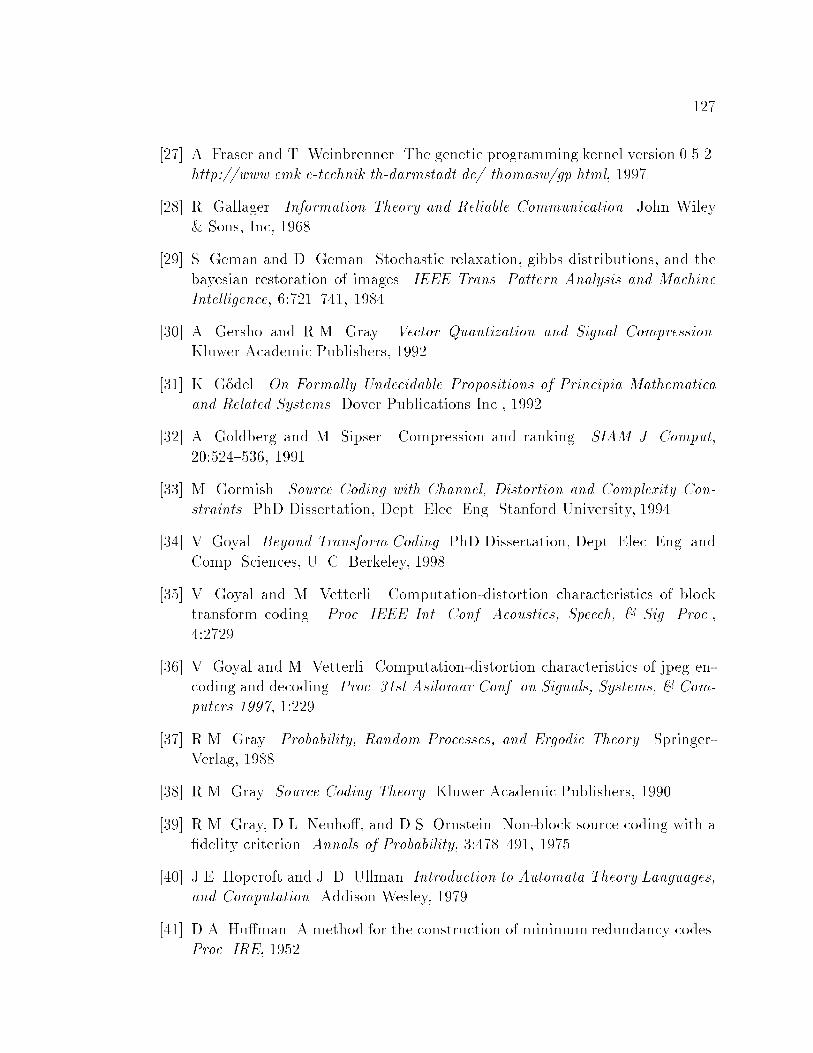
127

[27] A. Fraser and T. Weinbrenner. The genetic programming kernel version 0.5.2.

http://www.emk.e-technik.th-darmstadt.de/ thomasw/gp.html, 1997.

[28] R. Gallager. Information Theory and Reliable Communication. John Wiley& Sons, Inc, 1968.

[29] S. Geman and D. Geman. Stochastic relaxation, gibbs distributions, and the

bayesian restoration of images. IEEE Trans. Pattern Analysis and MachineIntelligence, 6:721{741, 1984.

[30] A. Gersho and R.M. Gray. Vector Quantization and Signal Compression.Kluwer Academic Publishers, 1992.

[31] K. G}odel. On Formally Undecidable Propositions of Principia Mathematicaand Related Systems. Dover Publications Inc., 1992.

[32] A. Goldberg and M. Sipser. Compression and ranking. SIAM J. Comput,

20:524{536, 1991.

[33] M. Gormish. Source Coding with Channel, Distortion and Complexity Con-straints. PhD Dissertation, Dept. Elec. Eng. Stanford University, 1994.

[34] V. Goyal. Beyond Transform Coding. PhD Dissertation, Dept. Elec. Eng. and

Comp. Sciences, U. C. Berkeley, 1998.

[35] V. Goyal and M. Vetterli. Computation-distortion characteristics of blocktransform coding. Proc. IEEE Int. Conf. Acoustics, Speech, & Sig. Proc.,

4:2729.

[36] V. Goyal and M. Vetterli. Computation-distortion characteristics of jpeg en-coding and decoding. Proc. 31st Asilomar Conf. on Signals, Systems, & Com-puters 1997, 1:229.

[37] R.M. Gray. Probability, Random Processes, and Ergodic Theory. Springer-Verlag, 1988.

[38] R.M. Gray. Source Coding Theory. Kluwer Academic Publishers, 1990.

[39] R.M. Gray, D.L. Neuho�, and D.S. Ornstein. Non-block source coding with a�delity criterion. Annals of Probability, 3:478{491, 1975.

[40] J.E. Hopcroft and J. D. Ullman. Introduction to Automata Theory Languages,and Computation. Addison Wesley, 1979.

[41] D.A. Hu�man. A method for the construction of minimum redundancy codes.Proc. IRE, 1952.

128

[42] R.C. Je�rey. Basic Problems in Methodology and Linguistics, chapter Mises

Redux, pages 213{222. 1977.

[43] A. Kolmogorov and V. Upsenkii. Algorithms and Randomness. SIAM Journal

Theory Probab. Appl., 32:3:389{412, 1987.

[44] A. N. Kolmogorov. Three Approaches to the Quantitative De�nition of Infor-mation. Problems Inform. Transmission, 1(1):1{7, 1965.

[45] A.N. Kolmogorov. Logical basis for information theory and probability theory.Trans. Inform. Theory, 1968.

[46] Y. Kontoyiannis. Pointwise redundancy in lossy data compression and uni-versal lossy data compression. IEEE Transactions on Information Theory,

46:136{152, 2000.

[47] J. Koza. Genetic Programming: On the Programming of Computers by Meansof Natural Selection. MIT Press., 1992.

[48] ed L. Torres and ed M. Kunt. Video Coding: The Second Generation Approach.Kluwer Academic, 1996.

[49] K. Lengwehasatit and A. Ortega. Distortion/decoding time tradeo�s in soft-ware dct-based image coding. Proc. IEEE Int. Conf. Acoustics, Speech, & Sig.

Proc., 4:2725.

[50] Sik K. Leung-Yan-Cheong and Thomas M. Cover. Some Equivalence BetweenShannon Entropy and Kolmogorov Complexity. IEEE Transactions on Infor-mation Theory, 24:331{339, 1978.

[51] L.A. Levin. Universal search problems. Problems Inform. Transmission,9:265{266, 1973.

[52] M. Li and P. Vitanyi. An Introduction to Kolmogorov Complexity and its

Apllications. Text and monographs in Computer Science Springer-Verlag, 2edition, 1997.

[53] Wineberg M and F. Oppacher. Parallel Problem Solving from Nature III, Vol866 of Lec. Notes in Computer Science, chapter A Representation Schemeto Perform Program Induction in a Canonical Genetic Algorithm. Springer-

Verlag, 1994.

[54] P. Martin-L}of. On the Concept of a Random Sequence. Theory Prob. Appl.,11, 1966.

129

[55] J. McCarthy. Automata Studies, Annals of Mathematical Studies, chapter The

Inversion of Functions De�ned by Turing Machines, pages 177{181. Num-ber 34. Princeton University Press, 1956.

[56] T.M. Mitchell. Machine Learning. Mc Graw-Hill, 1997.

[57] J. Muramatsu and F. Kanaya. Distortion Complexity and Rate-DistortionFunction. IEICE Trans. Fundamentals, E77-A, 1994.

[58] J. Muramatsu and F. Kanaya. Dual Quantity of the Distortion-Complexityand a Universal Data-Base for Fixed-Rate Data Compression with Distortion.

IEICE Trans. Fundamentals, E79-A, 1996.

[59] A.N. Netravali and B. G. Haskel. Digital Pictures: Representation, Compres-sion, and Standards, 2nd ed. Plenum Press, 1995.

[60] A. Nix and M.D. Vose. Modeling genetic algorithms with markov chains.Annals of Mathematics and Arti�cial Intelligence, 5:27{34, 1991.

[61] P. Nordin and W. Banzhaf. Programmatic compression of images and sound.

Proceedings of First International Conference on genetic Programming, 1996.

[62] C. Papadimitriou. Computational Complexity. Addison Wesley, 1994.

[63] A. Perez. Extensions of Shannon-McMillan's Limit Theorem to More General

Stochastic Processes. Trans. Third Prague Conf. on Inform. Theory, Statist.Decision Functions, and Random Processes, 1964.

[64] A. Puri and A. Eleftheriadis. Visual Communication and Image Processing,

chapter MPEG-4: An Object-Based Multimedia Coding Standard. MarcelDekker, 1998.

[65] J. Rissanen. Generalized Kraft inequality and arithmetic coding. IBM J. Res.Devel., 20.

[66] J. Rissanen. Stochastic Complexity in Statistical Inquiry. World Scienti�c,1989.

[67] G. Rudolph. Convergence analysis of canonical genetic algorithms. IEEE

Trans. Neural Networks, special issue on Evolutionary Computing, 5:96{101,Jan. 1994.

[68] A. Said and W. Pearlman. A new, fast, and e�cient image codec based on set

partitioning in hierarchical trees. IEEE Transactions on Circuits and Systemsfor Video Technology, 6:3:243{250, 1996.

130

[69] M. Schwartz. Information Transmission Modulation and Noise. McGraw-Hill,

4th edition, 1990.

[70] C.E Shannon. A Mathematical Theory of Communication. Bell SystemsTechnical Journal, 27, 1948.

[71] C.E. Shannon. Communication in presence of noise. Proc. IRE, 1949.

[72] C.E. Shannon. Coding theorems for a discrete source with �delity criterion.

IRE Nat. Conv. Rec., 1959.

[73] P.C. Shields. Universal Almost Sure Data Compression using Markov Types.Problems of Control and Information Theory, 19, 1990.

[74] G. E. Shilov and B. L. Gurevich. Integral Measure and Derivative: A Uni�edApproach. Prentice-Hall, 1966.

[75] A. Sinclair. Algorithms for Random Generation and Counting. Birkh}auser,1993.

[76] R. J. Solomono�. A Formal Theory of Inductive Inference, Part 1 and Part2. Inform. Contr., 7, 1964.

[77] R.J. Solomono�. Computational Learning Theory; Proc. 2nd European Conf.

Vol. 904 of Lec. Notes Arti�cial Intelligence,, chapter The Discovery of Algo-rithmic Probability, pages 1{18. Springer-Verlag, 1995.

[78] D. Sow and A. Eleftheriadis. On weighted universal image compression. sub-mitted to IEEE Trans. on Image Proc., December 1999.

[79] D. Sow and A. Eleftheriadis. Complexity distortion theory. submitted to IEEETrans. on Inf. Theory, June 2000.

[80] D. Sow and A. Eleftheriadis. Approximaton of the Resource Bounded Com-plexity Distortion Function. Proceedings 2000 IEEE International Symposium

on Information Theory, pages |, June 25 - July 1 2000.

[81] D. Sow and A. Eleftheriadis. Complexity Distortion Theory. Proceedings 1997IEEE International Symposium on Information Theory, page 188, June 29 -July 4 1997.

[82] D. Sow and A. Eleftheriadis. Representing Information with Computational

Resource Bounds. Proceedings 32nd Asilomar Conference on Signals, Systemsand Computers, November 1998.

131

[83] D. Sow and A. Eleftheriadis. Algorithmic Representation of Visual Informa-

tion. Proceedings 1997 IEEE International Conference on Image Processing,October 1997.

[84] R. Sun, J. Dayho�, and W. Weigand. A population-based search from geneticalgoritms through thermodynamic operation. Technical Reasearch Report,Institute for Systems Research, T.R.94-78, 1994.

[85] J. Suzuki. A markov chain analysis on simple genetic algorithms. IEEE Trans.on Systems, Man, and Cybernetics, 25:4:655{659, April 1995.

[86] J. Suzuki. A further result on the markov chain model of gas and their ap-plication to sa-like strategy. IEEE Trans. on Systems, Man, and Cybernetics,

pages 95{102, Feb. 1998.

[87] H.L. Van Trees. Detection Estimation, and Modulation Theory. John Wileyand Sons, 1968.

[88] A. Turing. On computable numbers with an application to the Entschei-dungsproblem.

[89] V.A. Upsensky and A. Shen. Relations between varieties of kolmogorov com-plexities. Mathematical Systems Theory, 29, 1996.

[90] M. Vetterli and J. Kovacevic. Wavelets and Subband Coding. Prentice-Hall,1995.

[91] P. Vitanyi. A discipline of evolutionary programming. Theoretical Computer

Science, to appear.

[92] P. Vitanyi and M. Li. Minimum Description Length Induction, Bayesianism,and Kolmogorov Complexity. IEEE Transactions on Information Theory,46:446.

[93] O. Watanabe. Kolmogorov Complexity and Computational Complexity.Springer-Verlag, 1992.

[94] W. Wulf, M. Shaw, and P. N. Hil�nger. Fundamental Structures of ComputerScience. Addison Wesley, 1981.

[95] A.D. Wyner, J. Ziv, and A.J. Wyner. On the role of pattern matching in

information theory. IEEE Transactions on Information Theory, 44.

[96] ed Y. Fisher. Fractal Image Compression. Springer Verlag, 1995.

132

[97] A. Sinclair Y. Rabani, Y. Rabinovich. A computational view of population

genetics. Proc, 27th ACM Symp. Theor. Comput., pages 83{92, 1995.

[98] E. Yang and S. Shen. Distortion Program-size Complexity with Respect to

a Fidelity Criterion and Rate Distortion Function. IEEE Transactions onInformation Theory, 39:288{292, 1993.

[99] E.H. Yang. The Proof of Levin's Conjecture. Chinese Sci. Bull., 34, 1989.

[100] ed Y.S. Abu-Mostafa. Complexity in Information Theory. Springer-Verlag,

1993.

[101] Z. Zhang and V.K.Wei. An on-line universal lossy data compression algorithm

via continuous codebook re�nement-Part I, 1996.

[102] J. Ziv. Coding for sources with unknown statistics: Part I. Probability of

error, 1972.

[103] J. Ziv. Coding for sources with unknown statistics: Part II. Distortion relativeto a �delity criterion, 1972.

[104] J. Ziv. Back from In�nity: A Constrained Resources Approach to Informa-tion Theory. Proceedings 1997 IEEE International Symposium on InformationTheory, page 4, 1997.

[105] A. K. Zvonkin and L. A. Levin. The Complexity of Finite Objects and TheDevelopment of the Concepts of Information and Randomness by Means ofthe Theory of Algorithms. Russian Math. Surveys, 25:6:83{124, 1970.

133

Appendix

A. Recursive Functions

One of the main results of Computability Theory is the equivalence between theformal conception of what an algorithm is and the intuitive notion of an e�ectiveprocedure. This equivalence is known as the Church-Turing thesis. A formal de�-

nition of what an algorithm is can be found in [17] using the concept of recursivefunction. Following the procedure proposed in [105], we can map �nite sequences,belonging to A�, to N . Functions on A� can then be seen as functions on N . ByF i, we denote a function with i arguments, F (x1; � � � ; xi); xj 2 A�; 1 � j � i. When

the number of arguments is clear from the context, we drop the superscript. Let C1,On, Inm be functions taking the following values: C1(x) = x+1, On(x1; � � � ; xn) = 0,Inm(x1; � � � ; xn) = xm.

De�nition 1 The operation of minimalization associates with each total functionfn+1(y; x1; � � � ; xn) the function hn(x1; � � � ; xn) whose value is the least value y, ifone such exists, for which

fn+1(y; x1; � � � ; xn) = 0

and which is unde�ned if no such y exists. We write:

hn(x1; � � � ; xn) = miny[fn+1(y; x1; � � � ; xn)]: (5.1)

De�nition 2 The function fn+1 is said to originate from the function gn and fromthe function hn+2 by a primitive recursion if for all natural numbers x1; � � � ; xn; y we

have:fn+1(x1; �; xn; 0) = g(x1; �; xn); (5.2)

fn+1(x1; �; xn; y + 1) = hn+2(x1; �; xn; y; fn+1(x1; �; xn; y)): (5.3)

134

De�nition 3 A function F is called partial recursive if it can be obtained from the

functions C1, On, Inm by a �nite number of operations of substitution (superposition),of primitive recursion and of minimalization2.

Note that there are many equivalent de�nitions for recursive functions using di�erent

primitive functions spanning the same space of functions. In all cases, an algorithmis just a recursive function that can be expressed by the construction mentioned inde�nition 3. In 1936 Alan Turing3 introduced the Turing machine (TM), a device

able to compute any recursive function. This device is a �nite state machine (FSM)with access to a �nite number of in�nite memory tapes on which the device canstore information. This device, although not practical, is widely accepted as themathematical model for computation because of the one to one mapping between

recursive functions and TM's. It is not a practical model because of the in�nitesize of its memory tape(s). Without memory, the device can only recognize regularlanguages. In order to accept context sensitive grammars, an in�nite amount ofmemory is required but at any time during the computation, the TM uses a �nite

amount of memory4. The Church-Turing-Thesis stating that anything that can bedone algorithmically can be performed by a Turing machine, justi�es the use of theTM as a model for computation. It clearly justi�es the substitution of the decoderin Shannon's classical communication system, by a Turing machine. It also makes

a step forward towards a uni�cation of all coding techniques, from traditional en-tropy methods which estimate relative frequencies, to novel approaches like fractalcoding or even model-based coding techniques. Another advantage is the potential

design of computer languages for representations. The use of such languages allowssemantical descriptions of information which is necessary to understand the infor-mation content. In this case, it seems more natural to use an algorithmic measureof information.

B. Randomness Tests

In this section, we follow the presentation made in [52] on randomness of individual

objects, �nite and in�nite.

2As mentioned in [105],partial recursive functions constructed without the minimalization oper-ation are de�ned everywhere. Only the operation of minimalization can lead to functions that arenot de�ned everywhere because this operation consisting of successive veri�cation of the validityof equation 5.1 might never stop.

3See [17] for detail description of Turing machines.4It is more accurate to say that the memory tapes are unbounded in size.

135

De�nition 1 Let P be a recursive probability measure on the sample space N . A

total function � : N �! N is a P -test (Martin-L}of test for randomness) if:

1. � is enumerable meaning that the set V = f(m;x) : �(x) � mg is recursivelyenumerable;

2.PfP (x) : �(x) � m; l(x) = ng � 2�m, for all n.

When applied to a sequence x, if �(x) � m, then from the second condition in theprevious de�nition, with probability 2�m, the sequence x is not random becauseit belongs to a small set Vm = fx : �(x) � mg, for m � 1 with small measure

and we recall that a random sequence must belong to a reasonable majority. Notethat it is assumed that P is recursive. It is hard to imagine what practical use itwould have to allow P not to be recursive. The critical regions associated with thecommon statistical tests are present in the form of the sequence V1 � V2 � � � � ;with Vm de�ned above.. Nesting is assured since �(x) � m + 1 implies �(x) � m.Also, note that each Vm is recursively enumerable from item 1 in de�nition 1. Thismeans that randomness testing at level m gives a certi�cate of non randomness fora sequence when �(x) � m. When �(x) � m, the result of the test is unknown.

The Kolmogorov complexity is an indicator for randomness. Sequences with shortdescriptions contain a good amount of regularities and should note be classi�edrandom. The machinery developed so far is still too weak to identify almost allregular sequences. To do so, we need the notion of universal test for randomness

De�nition 2 A universal Martin-L}of test for randomness with respect to measureP (universal P -test) is a test �0(: j P ) such that for each P -test �, there is a constantc, such that for all x, we have �0(x j P ) � �(x)� c.

A major result from this theory is the existence of a universal test. Any otherrandomness test cannot discover more than a constant amount of randomness. Thisfact also plays a central role in this thesis. It allows us to bridge Kolmogorovcomplexities with entropies. To make accurate statements about in�nite sequences,

we need the following de�nitions.

De�nition 3 Let � be a recursive probability measure on the space of in�nite se-quences, A1. A total function � : A1 �! N

Sf1g is a sequential �-test if:

1. �(w) = supn2Nf (xn1)g, where : N �! N is a total enumerable function

meaning that V = f(m; y) : (y) � mg is a recursively enumerable set;

2. �fx : �(x) � mg � 2�m, for each m � 0.

For a sequential �-test for randomness �, if �(x) =1, the sequence fails � and from

item 2 of de�nition 3, the set of x failing � has measure 0 respecting the typicalityproperty of random sequences.

136

De�nition 4 Let V be the set of all sequential �-tests. An in�nite binary sequence

x, or the binary represented real number 0:x, is called �-random if it passes allsequential �-tests:

x =2[V 2V

1\m=1

Vm (5.4)

where Vm =Sf�y : (m; y) 2 V g and V being de�ned in de�nition 3

The sets Vm are also called critical regions. By construction, they are nested:Vm � Vm+1; m = 1; 2; � � � From de�nition 3 we see that �(

T1m=1 Vm) = 0 and since V

is countably in�nite, �(SV2V

T1m=1 Vm) = 0. The sets

T1m=1 Vm and

SV2V

T1m=1 Vm

are respectively called constructive �-null set and maximal constructive �-null set.The de�nition of the universal sequential �-test is a direct consequence of this ob-servation.

De�nition 5 A universal sequential �-test f is a sequential �-test such that foreach sequential �-test �i, there is constant c � 0 and for all in�nite sequence x, we

have f(x) � �i(x)� c

De�nition 6 Let � be a probability measure on A1 and let �0(� j �) be a universalsequential �-test. An in�nite sequence x is �-random in the sense of Martin-L}of, if

�0(� j �) <1.

As mentioned earlier, the delimitation between random and non random sequencesis clearer for the in�nite case. We simply need a universal test and verify if the value

of the test is �nite or not. There are other ways to test sequences for randomness.The following type of test is used extensively to establish links between Shannon'sentropy and the Kolmogorov complexity.

De�nition 7 Let f be a unit integrable function over A1 with respect to � assumedrecursive. A function � is an integral-�-test i� �(!) = log f(!). It is a universalintegral �-test if it additively dominates all integral �-tests.

Integral tests are equivalent to sequential tests. If f is enumerable unit integrableover A1 with respect to �, then it can be shown that log f(�) is a sequential test.

Also, if � is a sequential �-test, then the function f de�ned by log f(!) = �(!) �2 log �(!) � c is an enumerable unit integrable function5. Of particular interest isthe following integral test which provides a link between Shannon's entropy andKolmogorov complexity.

5See [52] pp 287, lemma 4.5.7

137

Lemma 1 Let � be a recursive measure. Let ! 2 A1. The function

�0(! j �) = sup!2�x

f�C(x j �) � log2 �(x)g (5.5)

is a universal integral �-test6.

Proof: See [52].

2

Just like in the case of �nite sequences, this lemma shows that the di�erence betweenthe Kolmogorov complexity and the Shannon-Fano code length is an indicator ofrandomness. This result is at the heart of all equivalence results derived in chapter

3 and 4.

C. Markov Types

The Markov k-type is de�ned by sliding a window of length k + 1 along xn1 and

counting frequencies. These relative frequencies are then used to de�ne empiricaltransition probabilities.

De�nition 3 Let �x be the following in�nite sequence de�ned by:

�xtn+i = xi; i = 1; 2; � � � ; n; t = 0; 1; 2; � � � (5.6)

For each integer 0 � k < n and for each ak1 2 Ak, de�ne

pk(ak1) = lim

L!1

1

Lj fi : �xi+ki+1 = ak1; 0 � i < Lg j (5.7)

The periodicity of �x implies that

pk(ak1) =

1

nj fi : �xi+ki+1 = ak1; 0 � i < ng j (5.8)

andpk�1(a

k�11 ) =

Xak2A0

pk(ak1); a

k�11 2 Ak�1 (5.9)

6The x's in this de�nition are �nite sequences. They represent pre�xes of !. The value ofthe test is simply the supremum of the di�erence between the complexity of those pre�x and thelogarithm of their measure. This di�erence is simply the randomness de�ciency for �nite sequences.

138

De�nition 4 The Markov k-type of xn1 is the Markov measure �k with state space

Ak, stationary probabilities pk(ak1), and transition probabilities p(� j �) de�ned by:

p(ak+1 j ak1) =

pk+1(ak+11 )

pk(ak1)(5.10)

The entropy Hk of the k-type �k is given by:

Hk = �Xak+11

pk+1(ak+11 ) log2

pk+1(ak+11 )

pk(ak1)(5.11)

De�nition 5 The type class Tk(xn1) is de�ned as the set of all sequences of length

n with Markov type equal to the Markov type of xn1 .