All Shook Up: International Trade andFirm-level Volatility∗

PRELIMINARY AND INCOMPLETE

Christopher Kurz

Federal Reserve Board

Mine Senses

Johns Hopkins University

Andrei Zlate

Federal Reserve Bank of Boston

February 2017

Abstract

Despite the large theoretical literature on the macroeconomic dynamics arising frominternational trade, there is little theoretical research that rationalizes the relationshipbetween a firm’s trading patterns and its volatility. Our paper attempts to fill this gapby exploring the relationship between firms’ exporting and importing status and firm-level volatility in a dynamic, stochastic, general equilibrium model. We augment theframework with heterogeneous firms and endogenous exporting from Ghironi and Melitz(2005) to allow for international input sourcing. In this framework, we examine the firm-level volatility generated by the model for a cross-section of firm types, which are defined toreflect the rich heterogeneity in firms’international activities. In line with recent empiricalevidence on the link between a firm’s trade status and its volatility, the model predictionsare: (1) Exporters display lower volatility than non-exporters, whereas importers displayhigher volatility that non-importers. (2) Firms that trade for longer durations displaylower volatility than firms switching in and out of international trade. (3) Firms thatexport to uncorrelated foreign markets are less volatile, whereas firms importing fromuncorrelated foreign suppliers are more volatile.JEL classification: F16, F23, F41, L25Keywords: firm-level volatility; exporting; international sourcing; heterogeneous

firms; trade intensity; trade duration; diversification.

∗Contact: christopher.j.kurz@frb.gov, msenses@jhu.edu, andrei.zlate@bos.frb.org. The views in this paperare solely the responsibility of the authors and should not be interpreted as reflecting the views of the FederalReserve Bank of Boston, the Board of Governors of the Federal Reserve System, or of any other person associatedwith the Federal Reserve System.

1

1 Introduction

A large body of theoretical and empirical literature provides insight into the implications of

international trade for macroeconomic dynamics. By contrast, there is little work and a lack

of consensus regarding the impact of shocks passed through international trade on firm-level

characteristics. Recent work by Kurz and Senses (2016) documents a set of stylized facts on

the relationship between firm-level volatility and the trade exposure of a firm.

With the empirical foundations in hand, this paper attempts to fill the gap between the

theoretical research and stylized facts in order to rationalize the relationship between a firm’s

trading patterns and its volatility. We accomplish this through the framework of a dynamic,

stochastic, general equilibrium model of international macroeconomics and trade. We aug-

ment the framework with heterogeneous firms and endogenous exporting from Ghironi and

Melitz (2005, henceforth, GM05) to allow for international input sourcing, like in Zlate (2016).

Thus, our model consists of two economies, the North and the South. Each economy includes

one representative household and a continuum of firms– with each firm producing a different

variety– that are monopolistically competitive and heterogeneous in labor productivity. Both

Northern and the Southern firms produce for their domestic market and, similarly to GM05,

firms can serve overseas markets through exporting. In addition, the ability to offshore produc-

tion provides further flexibility, as certain Northern firms can choose to produce in the South

and import back to their domestic market.

In this framework, we examine the firm-level volatility generated by the model for a cross-

section of firm types, which are defined to reflect the rich heterogeneity in firms’international

activities. For this purpose, we define three types of representative firms according to their

exporting and importing status and persistence by focussing on different portions of the support

interval for firm-specific idiosyncratic productivity. Namely, we define representative firms that

are in the immediate vicinity of the endogenous productivity cutoff for exporting or importing,

and also representative firms that are well below or well above the corresponding cutoffs. Thus,

based on export status, the three representative firms are: the firm that never exports, the firm

that sometimes exports, and the firm that always exports. Based on import status, the three

representative firms are: the firm that never imports, the firm that sometimes imports, and the

firm that always imports. The resulting output is obtained by integrating and taking averages

2

over the varieties produced and endogenously exported or imported by each representative

firm. To compare the model implications for firm-level volatility to those from the data, we

simulate the model under various assumptions for the two-country bivariate process of aggregate

productivity, and compute model-generated impulse responses and measures of volatility for the

output and employment of the three types of exporting/importing firms.

In line with the empirical evidence, the model implies that, first, exporters display lower

volatility than non-exporters (at least for output), whereas importers display higher volatility

that non-importers. Second, firms that trade for longer durations display lower volatility than

firms switching in and out of international trade. Third, firms that export to uncorrelated

foreign markets are less volatile (at least for output), whereas firms importing from uncorrelated

foreign suppliers are more volatile (at least for employment). The model rationalizes these

findings by highlighting the asymmetry in the way that diversification across uncorrelated

trading partners affects exporters and importers: While diversification reduces the volatility

of exporters, as positive and negative shocks in the domestic and foreign markets offset each

other, it enhances the volatility of importers, since disruptions from one single supplier affects

the entire production process reliant on complementary inputs.

Taken together, this paper provides a theoretical rationale for the empirical evidence on the

link between exporting, importing, and firm-level volatility documented in Kurz and Senses

(2016). In addition, our paper adds to the recent body of theoretical literature that rational-

izes the impact of firms’decisions to export and/or import on either firm-level or macro-level

characteristics. However, most of this theoretical literature is silent on the impact of firms’

exporting and importing decisions on firm-level characteristics, although it devotes ample at-

tention to the impact on macro-level variables (see GM05, Alessandria and Choi, 2007; Contessi,

2015; Fattal Jaef and Lopez, 2014; Liao and Santacreu, 2015; Mandelman, 2016; Mandelman

and Zlate, 2015; Zlate, 2016). Among the scarce literature on firm-level characteristics, Fillat

and Garetto (2015) model the impact of firms’international status on firms’financial perfor-

mance, with firms engaging in exports and horizontal FDI displaying higher stock returns and

earning yields. Fillat, Garetto, and Oldenski (2015) also model the impact of host economy

characteristics on the risk premia of multinational firms.

The rest of the paper is organized as follows: Section 2 presents a set of stylized facts

relating trade and volatility. Section 3 introduces the baseline model with heterogeneous firms

3

and describes the firms’endogenous decisions to export and import. Section 4 translates the

model into an equivalent framework with three representative firms defined according to their

trade status and persistence. Section 5 presents the calibration. Section 6 discusses the results,

including impulse responses and moments describing the link between the firms’trade status

and the volatility of output and employment growth. Section 7 concludes.

2 Stylized Facts on Trading and Volatility

This section presents some basic empirical facts about the relationship between trade and

firm-level volatility.1 As mentioned, previous work by Kurz and Senses (2016) find significant

heterogeneity between the employment volatility between trading and non-trading firms, even

when accounting for firm-fixed effects. Moreover, there are substantial differences across firms

that trade, particularly across dimensions such as products traded, countries traded with, and

the time and duration of trade.

The data employed source from the Longitudinal Business Database (LBD) and the Longitu-

dinal Firm Trade Transactions Database (LFTTD). The LBD contains industry identification,

age, employment, firm identifiers, and longitudinal links and contains annual data on the uni-

verse of all private U.S. business establishments with paid employees from 1976 to present.

The LBD allows for a detailed analysis of employment dynamics and of the entry and exit of

establishments. Importantly, the longitudinal coverage and annual frequency of the LBD allows

for the calculation of firm-level volatility, which necessitates consecutive observations over time

for each firm.

We aggregate the establishment data from the LBD to the firm level and link it to the

LFTTD for the manufacturing sector. In addition to individual trade transactions of imports

and exports, the LFTTD includes information on the products traded (at the 10-digit Harmo-

nized Schedule (HS) level), the nominal value of the transaction, and the destination countries

for exports and source countries for imports.

The volatility measures we use capture the variability of growth rates of employment. We

calculate the growth rate of employment as the log difference in employment and use this

measure to calculate the volatility as the standard deviation of firm employment growth. For

1The results in this section will be expanded when additional output is disclosed by the Census Bureau.

4

this section, we employ data spanning 15 years from 1991 to 2005 and calculate firm-level

volatility for firms that report positive employment for at least five consecutive years over the

full 1991 to 2005 sample period. The resultant firm count is 331,874.

We first delineate the differences in employment volatility for firms that trade and those

that do not, and then further differentiate by temporary and permanent trading. We do this

for trading in general, that is, either importing or exporting, and also do this for exporters and

importers. The results of differentiating organizations by their trade status over volatility can

be found in figure 1. The top panel contains the average volatility for traders over four different

categories: Non traders, traders (i.e., firms that either import or export at least once over the

sample), temporary traders (i.e., organizations that do no trade every period), and permanent

traders. The four categories are repeated for exporters and importers in the next two panels of

figure 1.

As can be seen in figure 1, traders (either temporary or permanent) are less volatile than

non-traders, a result primarily driven by the low volatility of permanent traders. The average

volatility results can be further understood when decomposing trade status into importers and

exporters. For exporters (panel 2 in figure 1), exporters are less volatile than non-exporters,

and while this holds true for both temporary and permanent exporters, permanent exporters

tend to be less volatile than temporary exporters. For importers (panel 3 in figure 1), the result

is slightly different, with overall importers being more volatile than non-importers, a result

primarily driven by temporary importers.

The results in figure 1 imply that export and import status have differing implications for

an organization’s volatility. Putting this into the context of the transmission of international

shocks, trade may allow firms to diversify away from or to become exposed to international

volatility that amplifies or attenuates the variability to which the average domestic firm is

exposed. We will attempt to delineate these factors in our modeling and results section.

As figure 1 indicates, the amount of time traded has important implications for an organi-

zation’s volatility. A more stable trade status is directly related to lower volatility. Figure 2

addresses the relationship between a firm’s volatility and the time traded more directly. Specif-

ically, we plot the four quartiles of time traded for both exporters (blue bars) and importers

(red bars) over the second and third quartiles of trade shares. Trade share is the fraction of

exports to shipments for exporters and imports to intermediate inputs for importers. As can

5

be seen in both panels, there is a monotonic decline in volatility as firms increase the amount of

time they trade, for either exports or imports. As with trade status, we will attempt to model

such differences. In this case, drawing the distinction between organizations located near the

productivity cutoff for trading, and those well above the threshold, that is, permanent traders.

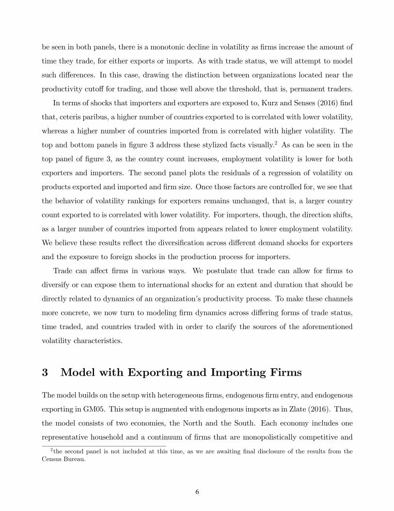
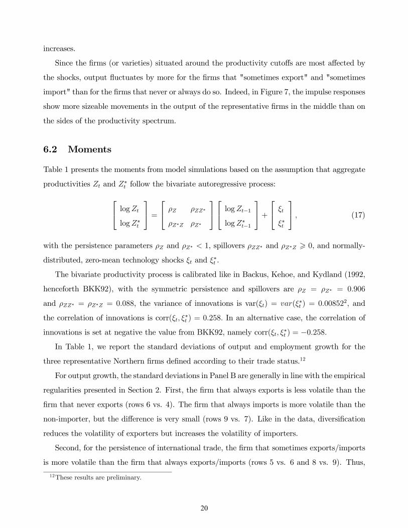
In terms of shocks that importers and exporters are exposed to, Kurz and Senses (2016) find

that, ceteris paribus, a higher number of countries exported to is correlated with lower volatility,

whereas a higher number of countries imported from is correlated with higher volatility. The

top and bottom panels in figure 3 address these stylized facts visually.2 As can be seen in the

top panel of figure 3, as the country count increases, employment volatility is lower for both

exporters and importers. The second panel plots the residuals of a regression of volatility on

products exported and imported and firm size. Once those factors are controlled for, we see that

the behavior of volatility rankings for exporters remains unchanged, that is, a larger country

count exported to is correlated with lower volatility. For importers, though, the direction shifts,

as a larger number of countries imported from appears related to lower employment volatility.

We believe these results reflect the diversification across different demand shocks for exporters

and the exposure to foreign shocks in the production process for importers.

Trade can affect firms in various ways. We postulate that trade can allow for firms to

diversify or can expose them to international shocks for an extent and duration that should be

directly related to dynamics of an organization’s productivity process. To make these channels

more concrete, we now turn to modeling firm dynamics across differing forms of trade status,

time traded, and countries traded with in order to clarify the sources of the aforementioned

volatility characteristics.

3 Model with Exporting and Importing Firms

The model builds on the setup with heterogeneous firms, endogenous firm entry, and endogenous

exporting in GM05. This setup is augmented with endogenous imports as in Zlate (2016). Thus,

the model consists of two economies, the North and the South. Each economy includes one

representative household and a continuum of firms that are monopolistically competitive and

2the second panel is not included at this time, as we are awaiting final disclosure of the results from theCensus Bureau.

6

heterogeneous in labor productivity. In both the North and the South, each firm produces a

different variety of goods for its domestic market, and some firms also produce domestically

to export like in GM05. In addition, some of the Northern firms can choose to produce either

domestically or offshore for their home market, like in Zlate (2016). Offshore production results

in the firm producing in the South and importing back to the North.

This section describes the problem of the Northern household and firms for the baseline

model with financial integration.3 The case for the South looks similar, except for the fact that

Southern firms do not produce offshore in the North and thus do not import.

3.1 Household’s Problem

The household maximizes expected lifetime utility: maxBt+1, xt+1

[Et∞∑s=t

βs−t C1−γs

1−γ

], where β ∈ (0, 1)

is the subjective discount factor, Ct is aggregate consumption, and γ > 0 is the inverse of the

inter-temporal elasticity of substitution. The budget constraint is:

(vt + dt)Ntxt + wtL+ (1 + rt)BN,t + (1 + r∗t )QtBS,t + Tt (1)

> vt (Nt +NE,t)xt+1 + Ct +BN,t+1 +QtBS,t+1 +π

2(BN,t+1)2 +

π

2Qt (BS,t+1)2 ,

The household starts every period with share holdings xt in a mutual fund of Nt firms whose

average market value is vt.4 It also holds risk-free, country-specific real bonds from the North

and the South, BN,t and BS,t, denominated in units of the issuing country’s consumption basket.

The holdings of Southern bonds are converted into units of the Northern basket through the

real exchange rate Qt.5 The household receives dividends equal to the average firm profit dt in

proportion with the stock of firms Nt, the real wage wt for L = 1 supplied inelastically, and

real rates of return rt and r∗t from the North and South-specific bonds.

Every period, the household purchases two types of assets. First, it purchases xt+1 shares in a

mutual fund of Northern firms, which includesNt incumbent firms producing either domestically

or offshore at time t, and also NE,t new firms that enter the market in period t. (Firm entry is

3"Baseline" refers to the model with fixed labor supply and no capital. Also, "financial integration" refersto the presence of risk-free, country-specific bonds traded internationally.

4Since stocks are not traded across countries, the equilibrium condition is xt = xt+1 = 1.5The real exchange rate Qt = P ∗t εt/Pt is the ratio between the price indexes in the South and the North

expressed in the same currency, where εt is the nominal exchange rate.

7

discussed in Section 2.2.) On average, each of these firms is worth its market value vt, equal to

the net present value of the expected stream of future profits. The household also purchases the

risk-free bonds BN,t+1 and BS,t+1. The budget allows for quadratic costs of adjustment for bond

holdings π2

(BN,t+1)2 and π2Qt (BS,t+1)2, which are rebated to the household as Tt. Parameter π

is set at a small value to ensure stationarity for net foreign assets in the presence of shocks.

The consumption basket includes varieties produced by the Northern firms domestically

(ω ∈ ΩNNt ), varieties produced by the Northern firms offshore and imported (ω ∈ ΩNS

t ), as well

as varieties produced by the Southern exporters (ω ∈ ΩSSt ), with the symmetric elasticity of

substitution θ > 1:

Ct =

zV,t∫zmin

yD,t(ω)θ−1θ dω

︸ ︷︷ ︸ω∈ΩNNt

+

∞∫zV,t

yV,t(ω)θ−1θ dω

︸ ︷︷ ︸ω∈ΩNSt

+

∞∫z∗X,t

y∗X,t(ω)θ−1θ dω

︸ ︷︷ ︸ω∈ΩSSt

θθ−1

, (2)

As explained in Section 2.3, [zmin,∞) is the support interval for the idiosyncratic productivity

of Northern firms, and only the more productive firms (with productivity above the endogenous

cutoff zV,t) choose to produce offshore and import back to the North.6 Since the number of firms

is time-variant and firms re-optimize their offshoring and exporting strategies every period, the

composition of the consumption basket changes over time. With the consumption basket Ct

set as numeraire, the price index for North is 1 =[∫ρt(ω)1−θdω

] 11−θ , in which ρt(ω) is the real

price of each variety and ω ∈ ΩNNt ∪ ΩNS

t ∪ ΩSSt .

The Euler equations for bonds are:

1 + πBN,t+1 = β(1 + rt+1)Et

[(Ct+1

Ct

)−γ], (3)

1 + πBS,t+1 = β(1 + r∗t+1)Et

[Qt+1

Qt

(Ct+1

Ct

)−γ], (4)

with the market-clearing conditions BN,t+1 +B∗N,t+1 = 0 and BS,t+1 +B∗S,t+1 = 0, in which the

asterisk denotes holdings by the Southern household of each type of bond. The Euler equation

6In the South, [z∗min,∞) is the support interval for the idiosyncratic productivity of Southern firms, and z∗X,tis the endogenous productivity cutoff for Southern exporters.

8

for stocks is below, with the rate of firm exit δ described in Section 2.2:

vt = β(1− δ)Et

[(Ct+1

Ct

)−γ(dt+1 + vt+1)

](5)

3.2 Firm Entry

Firm entry takes place every period in both the North and the South, as in GM05. In the

North, firm entry requires a sunk entry cost equal to fE units of Northern effective labor,

which reflects headquarter costs in the country of origin.7 After paying the sunk entry cost,

each firm is randomly assigned an idiosyncratic labor productivity factor z, which is drawn

independently from a common distribution G(z) with support over the interval [zmin,∞), and

which the firm keeps for the entire duration of its life. Thus, NE,t new firms are created every

period t and start producing at t + 1. However, all existing firms, including the new entrants,

are subject to a random exit shock that occurs with probability δ at the end of every period,

irrespective of their idiosyncratic productivity. The law of motion for the number of active

firms is: Nt+1 = (1− δ)(Nt +NE,t).

The potential entrants anticipate their expected post-entry value vt, which depends on

the expected stream of future profits dt, the stochastic discount factor, and the exogenous

probability δ of exit every period. The forward iteration of the Euler equation for stocks from

(5) generates the following expression for the expected post-entry value of the average firm:

vt = Et

∞∑s=t+1

[β(1− δ)]s−t(CsCt

)−γds

. (6)

Thus, every period, the unbounded pool of potential entrants face a trade-off between the sunk

entry cost and the expected stream of monopolistic profits. In equilibrium, firm entry takes

place until the expected value of the average firm is equal to the sunk entry cost: vt = fEwtZt.

3.3 Firms’Choice of Markets and Production Strategies

Every period, the active firms Nt choose endogenously the destination market(s) that they

serve and the location of production, as follows: (1) All firms serve their home market. For

7The sunk entry cost is equivalent to fEwt/Zt units of the Northern consumption basket.

9

this purpose, the Northern firms can either produce at home or produce offshore and import

the resulting output, like in Zlate (2016). Offshoring offers the advantage of a lower cost of

production but is subject to fixed and trade costs every period. Importantly, the firms’choice

between producing at home or offshore concerns output intended for the home market only,

and is not guided by access to the foreign market. (2) A subset of firms from each economy

also serve the foreign market. For this purpose, they produce domestically and export subject

to a fixed cost as in GM05. Each of these two problems (the offshoring decision of firms serving

their home market, and the exporting decision of firms serving the foreign market) are described

next.

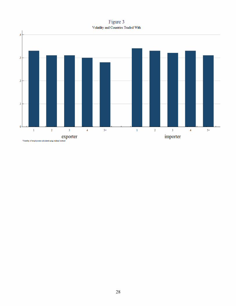
3.3.1 Importing

Every period, the Northern firm with idiosyncratic productivity z chooses between the two

possible production strategies to serve its home market: (a) Produce domestically, with out-

put yD,t(z) = Ztzlt(z) as a function of aggregate productivity Zt, the firm-specific labor pro-

ductivity z, and domestic labor lt(z). (b) Alternatively, produce inputs offshore and import

the resulting output, which then is used as input in production along with domestic inputs,

yV,t(z) = z [Ztlt(z)]α [Z∗t l∗t (z)]1−α . Thus, the firm producing offshore uses Southern labor l∗t (z)

and becomes subject to the aggregate Southern productivity Z∗, but carries its idiosyncratic

labor productivity z abroad.

Under monopolistic competition, the firm with idiosyncratic productivity z solves the profit-

maximization problem for the alternative scenarios of domestic and offshore production:

maxρD,t(z)

dD,t(z) = ρD,t(z)yD,t(z)− wtZtz

yD,t(z), (7)

maxρV,t(z)

dV,t(z) = ρV,t(z)yV,t(z)− τw∗tQt

Z∗t zyV,t(z)− fV

w∗tQt

Z∗t, (8)

where ρD,t(z) and ρV,t(z) are the prices associated with each of the two production strategies, wt

and w∗t are the real wages in the North and the South, and Qt is the real exchange rate. Thus,

the cost of producing one unit of output either domestically or offshore varies not only with the

cost of effective labor wt/Zt and w∗tQt/Z∗t across countries, but also with the idiosyncratic labor

productivity z across firms. In addition, the Northern firms producing offshore incur a fixed

10

cost equal to fV units of Southern effective labor, which reflects the building and maintenance

of the production facility offshore, and also an iceberg trade cost τ > 1 associated with the

importing of goods produced offshore back to the country of origin.8

The demand for the variety of firm z produced either domestically or offshore is yD,t(z) =

ρD,t(z)−θCt or yV,t(z) = ρV,t(z)−θCt respectively, where Ct is the aggregate consumption in

the North. Profit maximization implies the equilibrium prices ρD,t(z) = θθ−1

wtZtz

and ρV,t(z) =

θθ−1

τw∗tQtZ∗t z

for the alternative scenarios of domestic and offshore production. The corresponding

profits are dD,t(z) = 1θρD,t(z)1−θCt and dV,t(z) = 1

θρV,t(z)1−θCt − fV w∗tQt

Z∗t.

When deciding upon the location of production every period, the firm with productivity

z compares the profit dD,t(z) that it would obtain from domestic production with the profit

dV,t(z) that it would obtain from producing the same variety offshore. As a particular case, we

define the productivity cutoff level zV,t on the support interval [zmin,∞) such that the firm at

the cutoff obtains equal profits from producing domestically or offshore:

zV,t = z | dD,t(z) = dV,t(z) . (9)

The model implies that only the relatively more productive Northern firms find it profitable

to produce their varieties offshore. Despite the lower cost of effective labor in the South, only

firms with idiosyncratic productivity above the cutoff level (z > zV,t) obtain benefits from

offshoring that are large enough to cover the fixed and iceberg trade costs. This implication

is consistent with the empirical evidence in Kurz (2006), who shows that the U.S. plants and

firms using imported components in production are larger and more productive than their

domestically-oriented counterparts, as the larger idiosyncratic productivity levels allow them

to cover the fixed costs of offshoring.9 In addition, the productivity cutoff zV,t responds to

fluctuations in the relative cost of effective labor across countries. For any given level of firm-

specific productivity, a relatively lower cost of effective labor abroad implies higher profits

from offshoring, and therefore leads to a larger fraction of importing firms in equilibrium.

This implication is consistent with the empirical evidence on the determinants of offshoring

in Hanson, Mataloni, and Slaughter (2005), who show that U.S. multinationals import larger

8The fixed offshoring cost is equivalent to fV w∗t /Z∗t units of the Southern consumption basket.

9In Melitz (2003), more productive firms also have larger output and revenue.

11

shares of their foreign affi liates’s sales when the latter benefit from lower trade costs and lower

wages abroad.

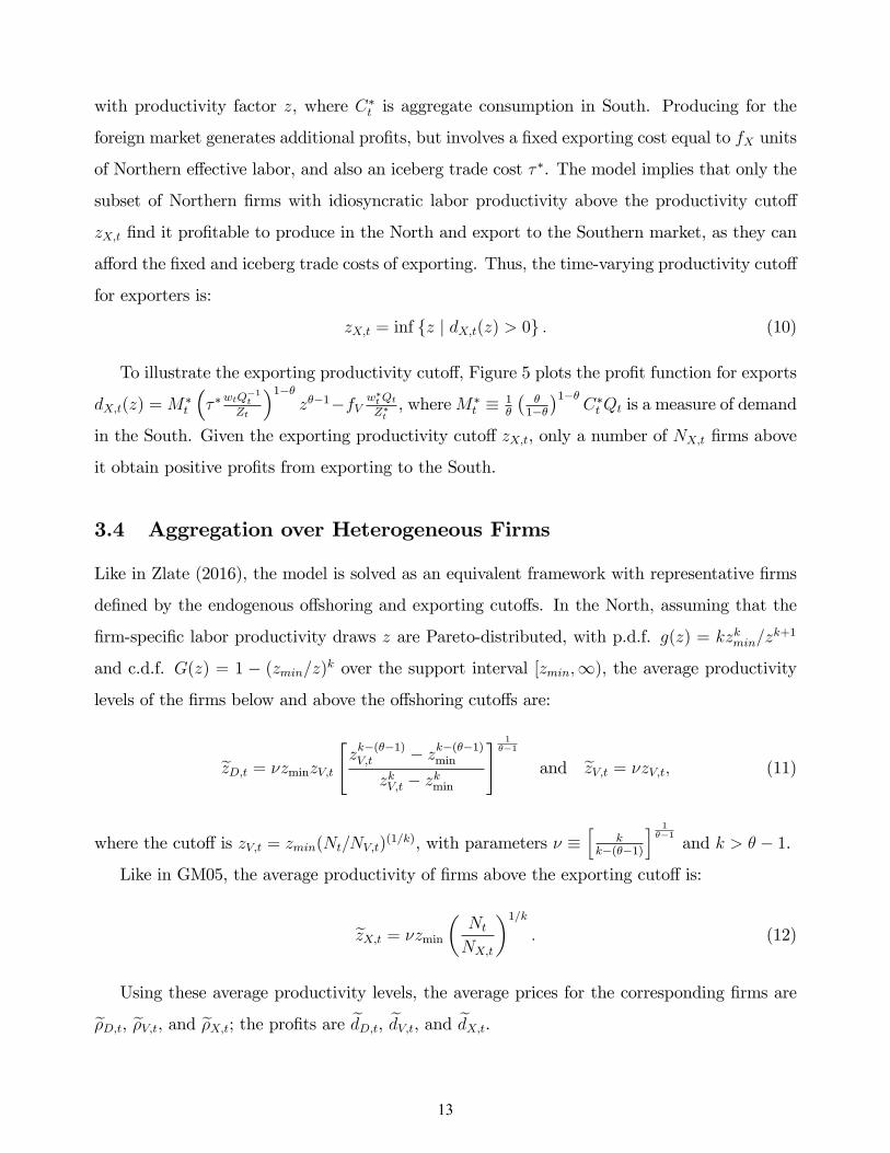
To illustrate the cutoff, Figure 4 shows the per-period profits from domestic and offshore pro-

duction as functions of the idiosyncratic productivity zθ−1 over the support interval [zmin,∞),

expressed as dD,t(z) = Mt

(wtZt

)1−θzθ−1 and dV,t(z) = Mt

(τw∗tQtZ∗t

)1−θzθ−1 − fV

w∗tQtZ∗t, where

Mt ≡ 1θ

(θ

1−θ)1−θ

Ct measures demand in the North. The vertical intercept is zero for domestic

production; it is equal to the negative of the fixed cost (−fV w∗tQtZ∗t) for offshoring. In this frame-

work, the productivity cutoff zV,t exists in equilibrium if the profit function from offshoring is

steeper than the profit function from domestic production, slope dV,t(z) > slope dD,t(z) .

When this condition is met, offshoring generates larger profits than domestic production for

a number of NV,t firms with idiosyncratic productivity along the upper range of the support

interval (z > zV,t).10

In equilibrium, the inequality of profit slopes described above is equivalent to τTOLt < 1,

with the "terms of labor" TOLt =Qtw∗t /Z

∗t

wt/Ztdefined as the ratio between the cost of effective labor

in the South and the North expressed in the same currency. (Note that an appreciation of the

terms of labor for the North is equivalent to a decline in TOLt.) In other words, the existence

of the productivity cutoff zV,t requires a cross-country asymmetry in the cost of effective labor,

whereby the effective wage in the South must be suffi ciently lower than in the North, so that

the difference covers the fixed and iceberg trade cost (τ > 1) and thus provides an incentive for

some of the Northern firms to produce offshore. The model calibration and the magnitude of

macroeconomic shocks ensure that this condition is satisfied every period.

3.3.2 Exporting

In addition to serving their domestic market, firms from each economy can choose to serve

the foreign market through exports, as in GM05. In the North, the firm with idiosyncratic

productivity z would use an amount of domestic labor lX,t(z) to produce for the Southern

market, yX,t(z) = ZtzlX,t(z). The Southern firms that choose to export to the North face

a similar problem. Profit maximization implies the following equilibrium price: ρX,t(z) =

θθ−1

τ ∗wtQ

−1t

Ztzand profit function: dX,t(z) = 1

θρX,t(z)1−θC∗tQt − fX wt

Ztfor the Northern exporter

10A second condition necessary to avoid the corner solution when all firms would produce offshore isdD,t(zmin) > dV,t(zmin). It ensures that zV,t > zmin in all periods.

12

with productivity factor z, where C∗t is aggregate consumption in South. Producing for the

foreign market generates additional profits, but involves a fixed exporting cost equal to fX units

of Northern effective labor, and also an iceberg trade cost τ ∗. The model implies that only the

subset of Northern firms with idiosyncratic labor productivity above the productivity cutoff

zX,t find it profitable to produce in the North and export to the Southern market, as they can

afford the fixed and iceberg trade costs of exporting. Thus, the time-varying productivity cutoff

for exporters is:

zX,t = inf z | dX,t(z) > 0 . (10)

To illustrate the exporting productivity cutoff, Figure 5 plots the profit function for exports

dX,t(z) = M∗t

(τ ∗

wtQ−1t

Zt

)1−θzθ−1−fV w∗tQt

Z∗t, whereM∗

t ≡ 1θ

(θ

1−θ)1−θ

C∗tQt is a measure of demand

in the South. Given the exporting productivity cutoff zX,t, only a number of NX,t firms above

it obtain positive profits from exporting to the South.

3.4 Aggregation over Heterogeneous Firms

Like in Zlate (2016), the model is solved as an equivalent framework with representative firms

defined by the endogenous offshoring and exporting cutoffs. In the North, assuming that the

firm-specific labor productivity draws z are Pareto-distributed, with p.d.f. g(z) = kzkmin/zk+1

and c.d.f. G(z) = 1 − (zmin/z)k over the support interval [zmin,∞), the average productivity

levels of the firms below and above the offshoring cutoffs are:

zD,t = νzminzV,t

[zk−(θ−1)V,t − zk−(θ−1)

min

zkV,t − zkmin

] 1θ−1

and zV,t = νzV,t, (11)

where the cutoff is zV,t = zmin(Nt/NV,t)(1/k), with parameters ν ≡

[k

k−(θ−1)

] 1θ−1

and k > θ − 1.

Like in GM05, the average productivity of firms above the exporting cutoff is:

zX,t = νzmin

(Nt

NX,t

)1/k

. (12)

Using these average productivity levels, the average prices for the corresponding firms are

ρD,t, ρV,t, and ρX,t; the profits are dD,t, dV,t, and dX,t.

13

3.5 Aggregate Accounting

Under financial integration, aggregate accounting implies that households spend their income

from labor, stock, and bond holdings on consumption and investment in new firms:

Ct +NE,tvt +BN,t+1 +QtBS,t+1 = wtL+Ntdt + (1 + rt)BN,t + (1 + r∗t )QtBS,t, (13)

C∗t +N∗E,tv∗t +Q−1

t B∗N,t+1 +B∗S,t+1 = w∗tL∗ +N∗t d

∗t + (1 + rt)Q

−1t B∗N,t + (1 + r∗t )B

∗S,t. (14)

The balance of international payments requires that the current account balance (i.e., the

trade balance, repatriated profits of offshore affi liates, and income from investments) equals the

change in bond holdings:

TBt+ NV,tdV,t︸ ︷︷ ︸Repatriated profits

+ rtBN,t + r∗tQtBS,t︸ ︷︷ ︸Income from bonds

= (BN,t+1 −BN,t) +Qt (BS,t+1 −BS,t)︸ ︷︷ ︸Change in bond holdings

, (15)

where the trade balance is given by:

TBt = NX,t (ρX,t)1−θ C∗tQt︸ ︷︷ ︸

Exports

−NV,t (ρV,t)1−θ Ct︸ ︷︷ ︸

Offshoring imports

−N∗X,t(ρ∗X,t

)1−θCt︸ ︷︷ ︸

Regular imports

(16)

Thus, the baseline model with financial integration for the Northern economy is character-

ized by 18 equations in 18 endogenous variables: Nt, ND,t, NV,t, NX,t, NE,t, dt, dD,t, dV,t, dX,t,

zD,t, zV,t, zX,t, vt, rt, wt, Ct, BN,t+1, and BS,t+1. Since the Southern firms do not produce in

the high-cost North, the Southern economy is described by only 13 equations in 13 endoge-

nous variables; there are no Southern counterparts for ND,t, NV,t, dV,t, zD,t and zV,t. Finally,

the real exchange rate Qt and the balance of international payments close the model. In this

framework, aggregate output in the North and the South are: Yt = Ct + NE,tvt + TBt and

Y ∗t = C∗t +N∗E,tv∗t + TB∗t , respectively.

4 Firms Defined by Trade Status and Persistence

The model with heterogeneous firms allows to define three types of representative Northern

firms along the dimensions highlighted in Kurz and Senses (2016). Namely, we differentiate

14

across firms according to their status as traders vs. non-traders; we also distinguish between

persistent vs. temporary traders. As such, for either importers and exporters, we define: (1)

the representative firm that never trades; (2) the firm that sometimes trades; and (3) the firm

that always trades. In this setup, the comparison of traders vs. non-traders concerns firm types

(3) vs. (1). The comparison of persistent vs. temporary traders involves types (3) vs. (2).

In this section, when referring to the continuum of heterogeneous firms over which the there

representative firms are defined, we refer to firms and varieties interchangeably since each firm

produces one variety. Thus, the three representative firms defined according to their importing

or exporting status and persistence represent averages taken over the range of heterogeneous

firms or varieties.

4.1 Importers

For importers, shown in Figure 4, we set the time-invariant productivity cutoffs zIM1 and zIM2

at one percent below and one percent above the steady-state value of the endogenous offshoring

cutoff zV,t. The magnitude of the stochastic shocks to aggregate productivity Z ensures that the

endogenous cutoff zV,t moves within the interval (zIM1, zIM2) without breaching its limits. In

turn, the time-invariant cutoffs define the three representative firms according to their import

status: (1) the firm that never imports, which represents the interval z < zIM1; (2) the firm

that sometimes imports, defined over zIM1 < z < zIM2; and (3) the firm that always imports,

over z > zIM2.

The output of each of these three representative firms is obtained by taking the average

productivity and output between the time-invariant cutoffs:

YIM_NEV,t =

[θ

θ − 1

wtZtzIM_NEV

]−θCt︸ ︷︷ ︸

Output produced at home

,

YIM_SOM,t =

(Nt −NIM_NEV,t −NV,t

NIM_SOM,t

)[θ

θ − 1

wtZtzIM_SOM(z<zV,t),t

]−θCt︸ ︷︷ ︸

Output produced at home when z<zV,t

+

+

(NV,t −NIM_ALW,t

NIM_SOM,t

)[θ

θ − 1

τw∗tQt

Z∗t zIM_SOM(z>zV,t),t

]−θCt︸ ︷︷ ︸

Output imported when z>zV,t

,

15

YIM_ALW,t =

[θ

θ − 1

τw∗tQt

ZtzIM_ALW

]−θCt︸ ︷︷ ︸

Output imported

,

where NIM_NEV,t, NIM_SOM,t, and NIM_ALW,t are the number of firms (or varieties) between

the time-invariant cutoffs zIM1 and zIM2. Also, parameters zIM_NEV , zIM_SOM , and zIM_ALW

are the corresponding average productivity levels. Since the cutoffs zIM1 and zIM2 are time-

invariant, the productivity averages between them are also time-invariant.

For the representative firm situated in the vicinity of the importing cutoff zV,t, output

depends on the share and average productivity levels of varieties produced domestically and

offshore. Since the importing cutoff zV,t moves within the interval (zIM1, zIM2) in response to

shocks, the share of varieties produced at home and offshore and their average productivity

levels also move over time, which enhances the volatility of output for the representative firm

around the offshoring cutoff. Thus, zIM_SOM(z<zV,t),t is the average productivity level over the

interval (zIM1, zV,t), while zIM_SOM(z>zX,t),t is the average productivity over (zV,t, zIM2).

Employment for each of the three representative firms is:

LIM_NEV,t =YIM_NEV,t

ZtzIM_NEV,

LIM_SOM,t =

(Nt −NIM_NEV,t −NV,t

NIM_SOM,t

)[θ

θ − 1

wtZtzIM_SOM(z<zV,t),t

]−θCt

ZtzIM_SOM(z<zV,t),t︸ ︷︷ ︸Labor hired at home for z<zV,t

+

+

(NV,t −NIM_ALW,t

NIM_SOM,t

)[θ

θ − 1

τw∗tQt

Z∗t zIM_SOM(z>zV,t),t

]−θCt

Z∗t zIM_SOM(z>zV,t),t︸ ︷︷ ︸Labor hired abroad for z>zV,t

,

LIM_ALW,t =YIM_ALW,t

Z∗t zIM_ALW︸ ︷︷ ︸Labor hired abroad

.

4.2 Exporters

In Figure 5, we also set the time-invariant productivity cutoffs zEX1 and zEX2 at one percent

below and one percent above the steady-state value of the exporting cutoff zX,t, which moves

within the interval without breaching it. As such, we define three representative firms according

to their export status: (1) the firm that never exports, (2) the firm that sometimes exports, and

16

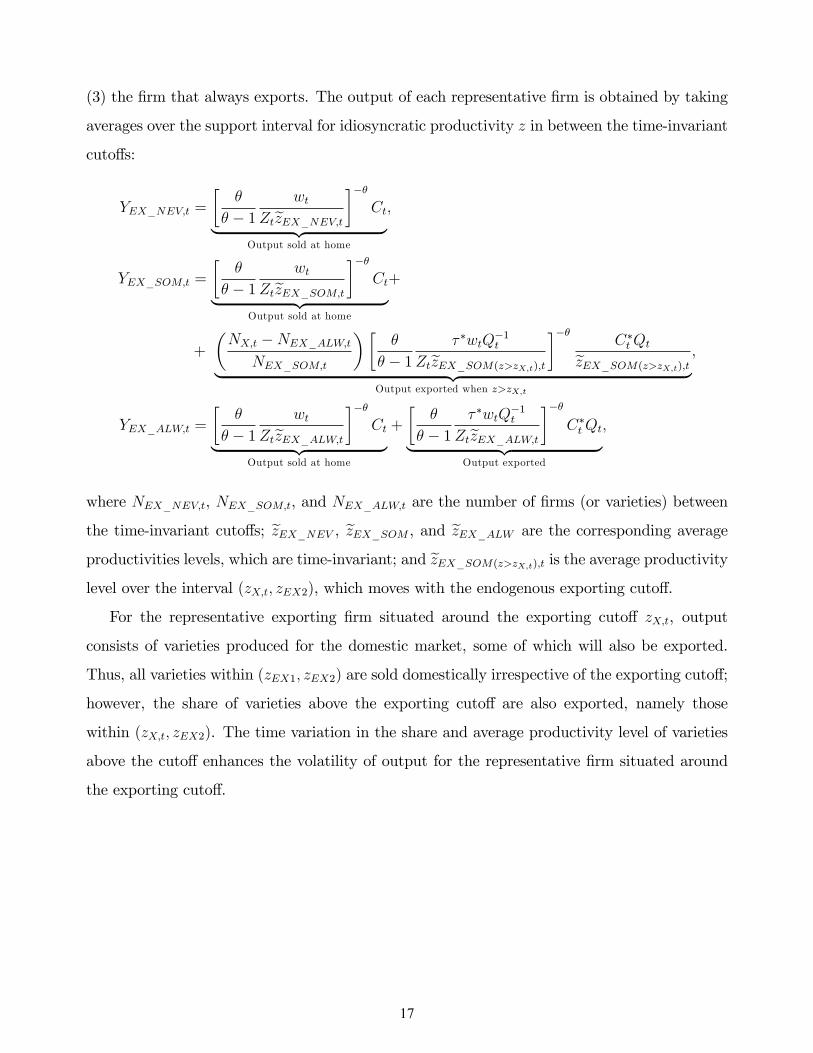
(3) the firm that always exports. The output of each representative firm is obtained by taking

averages over the support interval for idiosyncratic productivity z in between the time-invariant

cutoffs:

YEX_NEV,t =

[θ

θ − 1

wtZtzEX_NEV,t

]−θCt︸ ︷︷ ︸

Output sold at home

,

YEX_SOM,t =

[θ

θ − 1

wtZtzEX_SOM,t

]−θCt︸ ︷︷ ︸

Output sold at home

+

+

(NX,t −NEX_ALW,t

NEX_SOM,t

)[θ

θ − 1

τ ∗wtQ−1t

ZtzEX_SOM(z>zX,t),t

]−θC∗tQt

zEX_SOM(z>zX,t),t︸ ︷︷ ︸Output exported when z>zX,t

,

YEX_ALW,t =

[θ

θ − 1

wtZtzEX_ALW,t

]−θCt︸ ︷︷ ︸

Output sold at home

+

[θ

θ − 1

τ ∗wtQ−1t

ZtzEX_ALW,t

]−θC∗tQt︸ ︷︷ ︸

Output exported

,

where NEX_NEV,t, NEX_SOM,t, and NEX_ALW,t are the number of firms (or varieties) between

the time-invariant cutoffs; zEX_NEV , zEX_SOM , and zEX_ALW are the corresponding average

productivities levels, which are time-invariant; and zEX_SOM(z>zX,t),t is the average productivity

level over the interval (zX,t, zEX2), which moves with the endogenous exporting cutoff.

For the representative exporting firm situated around the exporting cutoff zX,t, output

consists of varieties produced for the domestic market, some of which will also be exported.

Thus, all varieties within (zEX1, zEX2) are sold domestically irrespective of the exporting cutoff;

however, the share of varieties above the exporting cutoff are also exported, namely those

within (zX,t, zEX2). The time variation in the share and average productivity level of varieties

above the cutoff enhances the volatility of output for the representative firm situated around

the exporting cutoff.

17

Employment for each of the three representative firms is:

LEX_NEV,t =YEX_NEV,t

ZtzEX_NEV,t,

LEX_SOM,t =

[θ

θ − 1

wtZtzEX_SOM,t

]−θCt

ZtzEX_SOM,t︸ ︷︷ ︸Labor hired for output sold at home

+

+

(NX,t −NEX−ALW,t

NEX−SOM,t

)[θ

θ − 1

τ ∗wtQ−1t

ZtzEX−SOM(z>zX,t),t

]−θC∗tQt︸ ︷︷ ︸

Labor hired for output exported when z>zX,t

,

LEX_ALW,t =YEX_ALW,t

ZtzEX_ALW,t.

In the presence of shocks, the growth of output and employment for each type of represen-

tative firm is computed as grYt = lnYt − lnYt−1 and grLt = lnLt − lnLt−1.

5 Calibration

We use a standard quarterly calibration by setting the subjective rate of time discount β = 0.99

to match an average annualized interest rate of 4 percent. The coeffi cient of relative risk

aversion is γ = 2. Following GM05, the intra-temporal elasticity of substitution is θ = 3.8 and

the probability of firm exit is δ = 0.025. The quadratic adjustment cost parameter for bond

holdings is π = 0.0025. The Pareto distribution parameter k, the iceberg trade cost τ , and

the fixed costs of offshoring (fV ) and exporting (fX and f ∗X) are calibrated so that the model

in steady state matches the importance of offshoring for the Mexican economy, as illustrated

by three empirical moments: (1) The maquiladora value added represents about 20 percent of

Mexico’s manufacturing GDP (Bergin, Feenstra, and Hanson, 2009) compared to 15 percent in

the model in steady state. (2) The maquiladora sector provided about 55 percent of Mexico’s

manufacturing exports on average from 2000 to 2006 (INEGI, 2008) compared to about 61

percent in the model. (3) The maquiladora sector accounts for about 25 percent of Mexico’s

manufacturing employment (Bergin, Feenstra, and Hanson, 2009) and 20 percent in the model.

To this end, I set k = 4.2, τ = 1.2, fV = 0.095, fX = 0.040, and f ∗X = 0.025.11 Without loss of

11The resulting exports-to-GDP ratios in steady state are 27 perecent for the North and 41 percent for theSouth. In the South, offshoring exports represent 61 percent of total exports and 25 percent of GDP.

18

generality, the lower bound of the support interval for firm-specific productivity in the North

and the South is zmin = z∗min = 1.

To obtain an asymmetric cost of effective labor across countries in steady state, the sunk

entry cost, which reflects headquarter costs sensitive to the regulation of starting a business in

the firms’country of origin, is set to be larger in the South than in the North (f ∗E = 4fE and

fE = 1). As a result, the steady-state output, the number of firms, the labor demand, and

the effective wage are relatively lower in the South. The calibration reflects the considerable

variation in the monetary cost of starting a business across economies, which was 2.8 times

higher in Mexico than in the United States in purchasing power parity terms in 2010 (World

Bank, 2011). The asymmetric sunk entry costs, along with the values for k, τ , fV , fX , and

f ∗X discussed above, generate a steady-state value for the terms of labor that is less than unit

(TOL = Qw∗/Z∗

w/Z= 0.75). In other words, the steady-state cost of effective labor in the South is

75 percent of the cost of effective labor in the North. Thus, the calibration provides an incentive

for some of the Northern firms to produce offshore in steady state.

6 Results

6.1 Impulse Responses

To understand the behavior of the endogenous productivity cutoffs zV,t and zX,t that drive the

firms’importing and exporting decisions, we compute impulse responses for key variables to a

transitory one-percent increase in aggregate productivity in the North. Aggregate productivity

follows the autoregressive process logZt+1 = ρ logZt + ξt, with persistence ρ = 0.9.

As shown in Figure 6, the shock to aggregate productivity in the North causes firm entry

and the number of established firms to increase. Firm entry puts upward pressure on the real

wage in the North, which causes the terms of labor to appreciate (i.e., the cost of effective labor

in the North to increase relative to the South), as shown by the terms of labor falling below

the steady state. Due to the cost of effective labor appreciating in the North, the exporting

cutoff zX,t rises and the fraction of exporting firms NX/N declines before returning to their

steady-state levels. Also, the importing cutoff zV,t falls on impact and persists below its steady

state (despite a short-lived recovery), which implies that the fraction of importing firms NV /N

19

increases.

Since the firms (or varieties) situated around the productivity cutoffs are most affected by

the shocks, output fluctuates by more for the firms that "sometimes export" and "sometimes

import" than for the firms that never or always do so. Indeed, in Figure 7, the impulse responses

show more sizeable movements in the output of the representative firms in the middle than on

the sides of the productivity spectrum.

6.2 Moments

Table 1 presents the moments from model simulations based on the assumption that aggregate

productivities Zt and Z∗t follow the bivariate autoregressive process: logZt

logZ∗t

=

ρZ ρZZ∗

ρZ∗Z ρZ∗

logZt−1

logZ∗t−1

+

ξt

ξ∗t

, (17)

with the persistence parameters ρZ and ρZ∗ < 1, spillovers ρZZ∗ and ρZ∗Z > 0, and normally-

distributed, zero-mean technology shocks ξt and ξ∗t .

The bivariate productivity process is calibrated like in Backus, Kehoe, and Kydland (1992,

henceforth BKK92), with the symmetric persistence and spillovers are ρZ = ρZ∗ = 0.906

and ρZZ∗ = ρZ∗Z = 0.088, the variance of innovations is var(ξt) = var(ξ∗t ) = 0.008522, and

the correlation of innovations is corr(ξt, ξ∗t ) = 0.258. In an alternative case, the correlation of

innovations is set at negative the value from BKK92, namely corr(ξt, ξ∗t ) = −0.258.

In Table 1, we report the standard deviations of output and employment growth for the

three representative Northern firms defined according to their trade status.12

For output growth, the standard deviations in Panel B are generally in line with the empirical

regularities presented in Section 2. First, the firm that always exports is less volatile than the

firm that never exports (rows 6 vs. 4). The firm that always imports is more volatile than the

non-importer, but the difference is very small (rows 9 vs. 7). Like in the data, diversification

reduces the volatility of exporters but increases the volatility of importers.

Second, for the persistence of international trade, the firm that sometimes exports/imports

is more volatile than the firm that always exports/imports (rows 5 vs. 6 and 8 vs. 9). Thus,

12These results are preliminary.

20

proximity to the productivity cutoffs enhances the volatility of temporary exporters/importers

relative to that of firms that trade consistently.

Third, regarding the effect of diversification, the exporting firm (row 6) ismore volatile when

it trades with a foreign destination that is positively correlated with the home economy (column

1) than negatively correlated (column 2). As such, export diversification across uncorrelated

destinations reduces volatility, since positive shocks to foreign demand may offset negative

shocks at home. Unlike in the data, the importing firm (row 9) is also more volatile when it

relies on foreign sources that are positively correlated with the home economy (column 1) than

negatively correlated (column 2).

These results also hold for employment growth, presented in Panel C, although with some

exceptions. Unlike in the data, the volatility of firms than always export exceeds that of firms

who do not (rows 12 vs. 10); and export diversification across uncorrelated markets does not

reduce volatility (row 12, columns 1 vs. 2). However, consistent with the data, importers are

more volatile than non-importers (rows 15 vs. 13); firms around the cutoffs are more volatile

than those further above (rows 11 vs. 12 and 14 vs. 15); and diversification across uncorrelated

sources enhances the volatility of importers (row 15).

In next steps, we will study the impact of diversification across import sources on firm-level

volatility in a setup that allows for complementarity between domestic and imported inputs.

We will also study the impact of international trade on the volatility of firms that export and

import simultaneously. Diversification across a larger number of trade partners will be modeled

explicitly rather than proxied by calibrating a negative correlation of shocks. Finally, we will

document the impact of the prevalence of exporting and importing firms on aggregate volatility.

7 Conclusion

This paper is predicated upon a set of stylized facts presented in Kurz and Senses (2016) which

point to considerable heterogeneity in the volatility of firms that differ in terms of the level of

engagement in international trade, the type of products they trade, and the characteristics of

their trading partners. In particular, Kurz and Senses (2016) find that importers experience

higher levels of volatility compared to non-trading firms. This relationship is mainly driven

by firms that switch in and out of importing. Firms that only export experience lower levels

21

of volatility. These results are complemented with findings that indicate firm-level volatility

increases with a larger share of exports and imports and is depended on the number of products

traded and the number of countries traded with.

In contrast to the large body of theoretical and empirical literature on international trade’s

implications for macroeconomic dynamics, there is little theoretical work regarding the trans-

mission of international shocks to firm-level volatility. Our paper attempts to fill this gap

by exploring the relationship between firms’ exporting and importing status and firm-level

characteristics– namely the volatility of output and employment– in a dynamic, stochastic,

general equilibrium model of international macroeconomics and trade. We augment the hetero-

geneous firms and endogenous exporting framework of GM05 to allow for international input

sourcing. More specifically, we examine the firm-level volatility generated by the model for a

cross-section of firm types, which are defined to reflect the rich heterogeneity in firms’interna-

tional activities.

In line with the empirical evidence, the model predictions are: (1) Exporters display lower

volatility than non-exporters (at least for output), whereas importers display higher volatility

that non-importers. (2) Firms that trade for longer durations display lower volatility than

firms switching in and out of international trade. (3) Firms that export to uncorrelated foreign

markets are less volatile (at least for output), whereas firms importing from uncorrelated foreign

suppliers are more volatile (at least for employment). The model rationalizes these findings by

highlighting the asymmetry in the way that diversification across uncorrelated trading partners

affects exporters and importers: While diversification reduces the volatility of exporters, as

positive and negative shocks in destination markets offset each other, it enhances the volatility

of importers, since disruptions from one single supplier affects the entire production process

reliant on complementary inputs.

8 List of References

References

[1] Alessandria, George and Horag Choi. 2007. "Do sunk costs of exporting matter for net

export dynamics?" Quarterly Journal of Economics, 122(1): 289-336.

22

[2] Backus, David K.; Patrick J. Kehoe; and Finn E. Kydland, 1992. "International real

business cycles." Journal of Political Economy, 100(4): 745-775.

[3] Contessi, Silvio. 2015. "Multinational firms’entry and productivity: Some aggregate impli-

cations of firm-level heterogeneity." Journal of Economic Dynamics and Control, 61(2015):

61-80.

[4] Fattal Jaef, Roberto N. and Jose Ignacio Lopez. 2014. "Entry, trade costs and international

business cycles." Journal of International Economics, 94: 224-238.

[5] Fillat, Jose L. and Stefania Garetto. 2015. "Risk, returns, and multinational production."

Quarterly Journal of Economics, 130(4): 2027-2073.

[6] Fillat, Jose L.; Stefania Garetto; and Lindsay Oldenski. 2015. "Diversification, cost struc-

ture, and the risk premium of multinational corporations." Journal of International Eco-

nomics, 96: 37-54.

[7] Ghironi, Fabio and Marc J. Melitz. 2005. "International trade and macroeconomic dynam-

ics with heterogeneous firms." Quarterly Journal of Economics, 120(3): 865-915.

[8] Hanson, Gordon H.; Raymond J. Mataloni; and Matthew J. Slaughter. 2005. "Vertical

production networks in multinational firms." Review of Economics and Statistics, 87(4):

664-678.

[9] Kurz, Christopher. 2006. "Outstanding outsourcers: A firm- and plant-level analysis of

production sharing." FEDs Working Paper No. 2006-04.

[10] Kurz, Christopher and Mine Z. Senses. 2016. "Importing, exporting, and firm-level em-

ployment volatility." Journal of International Economics, 98: 160-175.

[11] Liao, Wi and Ana Maria Santacreu. 2015. "The trade comovement puzzle and the margins

of international trade." Journal of International Economics, 96: 266-288.

[12] Mandelman, Federico. 2016. "Labor market polarization and international macroeconomic

dynamics." Journal of Monetary Economics, forthcoming.

23

[13] Mandelman, Federico and Andrei Zlate. 2016. "Offshoring, low-skilled immigration, and

labor market polarization." Federal Reserve Banks of Atlanta and Boston, mimeo.

[14] Melitz, Marc. 2003. “The impact of trade on intra-industry reallocations and aggregate

industry productivity.”Econometrica, 71(6): 1695-1725.

[15] Zlate, Andrei. 2016. "Offshore production and business cycle dynamics with heterogeneousfirms." Journal of International Economics, forthcoming 2016.

24

Table 1: Moments

TFP calibration as in BKK92corr(ε, ε∗) > 0 corr(ε, ε∗) < 0

A. St. dev. (%), aggr. variables, levels (1) (2)1. Y 0.97 0.922. C (relative to Y ) 0.67 0.553. NE (relative to Y ) 3.52 4.37B. St. dev. (%), output growth

Exporters:4. grYEX−NEV (never) 0.46 0.365. grYEX−SOM (sometimes) 5.31 4.166. grYEX−ALW (always) 0.43 0.33

Importers:7. grYIM−NEV (never) 0.46 0.368. grYIM−SOM (sometimes) 11.39 9.249. grYIM−ALW (always) 0.47 0.37C. St. dev. (%), employment growth

Exporters:10. grLEX−NEV (never) 0.51 0.6211. grLEX−SOM (sometimes) 4.79 3.9312. grLEX−ALW (always) 0.58 0.72

Importers:13. grLIM−NEV (never) 0.51 0.6214. grLIM−SOM (sometimes) 9.11 7.4115. grLIM−ALW (always) 0.66 0.83D. International correlations, levels16. Y, Y ∗ 0.42 −0.0817. Y, TB/Y −0.18 −0.1418. Z,Z∗ 0.31 −0.20

25

26

27

28

Table 1: Moments

TFP calibration as in BKK92corr(ε, ε∗) > 0 corr(ε, ε∗) < 0

A. St. dev. (%), aggr. variables, levels (1) (2)1. Y 0.97 0.922. C (relative to Y ) 0.67 0.553. NE (relative to Y ) 3.52 4.37B. St. dev. (%), output growth

Exporters:4. grYEX−NEV (never) 0.46 0.365. grYEX−SOM (sometimes) 5.31 4.166. grYEX−ALW (always) 0.43 0.33

Importers:7. grYIM−NEV (never) 0.46 0.368. grYIM−SOM (sometimes) 11.39 9.249. grYIM−ALW (always) 0.47 0.37C. St. dev. (%), employment growth

Exporters:10. grLEX−NEV (never) 0.51 0.6211. grLEX−SOM (sometimes) 4.79 3.9312. grLEX−ALW (always) 0.58 0.72

Importers:13. grLIM−NEV (never) 0.51 0.6214. grLIM−SOM (sometimes) 9.11 7.4115. grLIM−ALW (always) 0.66 0.83D. International correlations, levels16. Y, Y ∗ 0.42 −0.0817. Y, TB/Y −0.18 −0.1418. Z,Z∗ 0.31 −0.20

25

26

27

Figure 4: Importing firms.

Figure 5: Exporting firms.

NV,t

importing firms

21

NIM-SOM,t firms, sometimes import

NIM-ALW,t firms, always import

,

,

0

∗

∗

,

NIM-NEV,t firms, never import

21 1

1

NX,t

exporting firms

NEX-SOM,t firms, sometimes export

NEX-ALW,t firms, always export

NEX-NEV,t firms, never export

,

,

0

29

Figure 6: Impulse responses: the exporting and importing productivity cutoffs.

Figure 7: Impulse responses: the output of representative firms.

30