all
DESCRIPTION
gTRANSCRIPT

Computer Science 3725
Winter Semester, 2015
1

Pipelining — Instruction Set Parallelism (ISP)
Pipelining is a technique which allows several instructions to over-
lap in time; different parts of several consecutive instructions are
executed simultaneously.
The basic structure of a pipelined system is not very different from
the multicycle implementation previously discussed.
In the pipelined implementation, however, resources from one cycle
cannot be reused by another cycle. Also, the results from each stage
in the pipeline must be saved in a pipeline register for use in the next
pipeline stage.
The following page shows the potential use of memory in a pipelined
system where each pipeline stage does the operations corresponding
to one of the cycles identified previously.
2

A pipelined implementation
IF
RD
ALU
MEM
WB
0 1 2 3 4 5 6 7 8 9 10 11 12 13
time (clock cycles)
Note that two memory accesses may be required in each machine
cycle (an instruction fetch, and a memory read or write.)
How could this problem be reduced or eliminated?
3

What is required to pipeline the datapath?
Recall that when the multi-cycle implementation was designed, in-
formation which had to be retained from cycle to cycle was stored in
a register until it was needed.
In a pipelined implementation, the results from each pipeline stage
must be saved if they will be required in the next stage.
In a multi-cycle cycle implementation, resources could be “shared”
by different cycles.
In a pipelined implementation, every pipeline stage must have all the
resources it requires on every clock cycle.
A pipelined implementation will therefore require more hardware
than either a single cycle or a multicycle implementation.
A reasonable starting point for a pipelined implementation would be
to add pipeline registers to the single cycle implementation.
We could have each pipeline stage do the operations in each cycle of
the multi-cycle implementation.
4

Note that in a pipelineds implementation, every instruction passes
through each pipeliner stage. This is quite different from the multi-
cycle implementation, where a cycle is omitted if it is not required.
For example, this means that for every instruction requiring a reqister
write, this action happens four clock periods after the instruction is
fetched from instruction memory.
Furthermore, if an instruction requires no action in a particular
pipeline stage, any information required required by a later stage
must be “passed through.”
A processor with a reasonably complex instruction set may require
much more logic for a pipelined implementation than for a multi-cycle
implementation.
The next figure shows a first attempt at the datapath with pipeline
registers added.
5

MUX
0
1
dataWrite
RegisterWrite
ReadRegister 2
Register 1Read
Readdata 1
Readdata 2
dataWrite
Readdata
MemoryData
MUX
0
1
extendSign
MUX
0
1
Shiftleft 2
Add
Instruction[31−0]
MemoryInstruction
addressReadPC
Add
4
UX
1
0
M
EX MEMIF WBID
ALUZeroRegisters
Address
Inst[15−11]
Inst[20−16]
Inst[25−21]
3216
Inst[15−0]
6

It is useful to note the changes that have been made to the datapath,
The most obvious change is, of course, the addition of the pipeline
registers.
The addition of these registers introduce some questions.
How large should the pipeline registers be?
Will they be the same size in each stage?
The next change is to the location of the MUX that updates the PC.
This must be associated with the IF stage. In this stage, the PC
should also be incremented.
The third change is to preserve the address of the register to be
written in the register file. This is done by passing the address along
the pipeline registers until it is required in the WB stage.
The output of the MUX which provides the write address is now the
pipeline register.
7

Pipeline control
Since five instructions are now executing simultaneously, the con-
troller for the pipelined implementation is, in general, more complex.
It is not as complex as it appears on first glance, however.
For a processor like the MIPS, it is possible to decode the instruction
in the early pipeline stages, and to pass the control signals along the
pipeline in the same way as the data elements are passed through
the pipeline.
(This is what will be done in our implementation.)
A variant of this would be to pass the instruction field (or parts of
it) and to decode the instruction as needed for each stage.
For our processor example, since the datapath elements are the same
as for the single cycle processor, then the control signals required
must be similar, and can be implemented in a similar way.
All the signals can be generated early (in the ID stage) and passed
along the pipeline until they are required.
8

controlALU
BW
BW
BWM
EM
MEM
E
X
Inst[5−0]
RegDst
MemtoReg
RegWrite
Branch
MemWrite
MemRead
PCSrc
Inst [31−26]
ALUSrc
ALUop
MUX
0
1
dataWrite
RegisterWrite
ReadRegister 2
Register 1Read
Readdata 1
Readdata 2
dataWrite
Readdata
MemoryData
MUX
0
1
extendSign
Shiftleft 2
Add
Instruction[31−0]
MemoryInstruction
addressReadPC
EX MEMIF WBID
Add
4
UX
1
0
M
MUX
0
1
ALUZeroRegisters
Address
Inst[15−11]
Inst[20−16]
Inst[25−21]
3216
Inst[15−0]
9

Executing an instruction
In the following figures, we will follow the execution of an instruction
through the pipeline.
The instructions we have implemented in the datapath are those of
the simplest version of the single cycle processor, namely:
• the R-type instructions
• load
• store
• beq
We will follow the load instruction, as an example.
10

controlALUInst[5−0]
MUX
0
1
dataWrite
RegisterWrite
ReadRegister 2
Register 1Read
Readdata 1
Readdata 2
dataWrite
Readdata
MemoryData
MUX
0
1
extendSign
Shiftleft 2
Add
Instruction[31−0]
MemoryInstruction
addressReadPC
EX MEMIF WBID
Add
4
UX
1
0
M
MUX
0
1
ALUZeroRegisters
Address
Inst[15−11]
Inst[20−16]
Inst[25−21]
3216
Inst[15−0]
IF/ID ID/EX EX/MEM MEM/WB
11

controlALUInst[5−0]
MUX
0
1
dataWrite
RegisterWrite
ReadRegister 2
Register 1Read
Readdata 1
Readdata 2
dataWrite
Readdata
MemoryData
MUX
0
1
extendSign
Shiftleft 2
Add
Instruction[31−0]
MemoryInstruction
addressReadPC
EX MEMIF WBID
Add
4
UX
1
0
M
MUX
0
1
ALUZeroRegisters
Address
Inst[15−11]
Inst[20−16]
Inst[25−21]
3216
Inst[15−0]
IF/ID ID/EX EX/MEM MEM/WB
12

controlALUInst[5−0]
MUX
0
1
dataWrite
RegisterWrite
ReadRegister 2
Register 1Read
Readdata 1
Readdata 2
dataWrite
Readdata
MemoryData
MUX
0
1
extendSign
Shiftleft 2
Add
Instruction[31−0]
MemoryInstruction
addressReadPC
EX MEMIF WBID
Add
4
UX
1
0
M
MUX
0
1
ALUZeroRegisters
Address
Inst[15−11]
Inst[20−16]
Inst[25−21]
3216
Inst[15−0]
IF/ID ID/EX EX/MEM MEM/WB
13

controlALUInst[5−0]
MUX
0
1
dataWrite
RegisterWrite
ReadRegister 2
Register 1Read
Readdata 1
Readdata 2
dataWrite
Readdata
MemoryData
MUX
0
1
extendSign
Shiftleft 2
Add
Instruction[31−0]
MemoryInstruction
addressReadPC
EX MEMIF WBID
Add
4
UX
1
0
M
MUX
0
1
ALUZeroRegisters
Address
Inst[15−11]
Inst[20−16]
Inst[25−21]
3216
Inst[15−0]
IF/ID ID/EX EX/MEM MEM/WB
14

controlALUInst[5−0]
MUX
0
1
dataWrite
RegisterWrite
ReadRegister 2
Register 1Read
Readdata 1
Readdata 2
dataWrite
Readdata
MemoryData
MUX
0
1
extendSign
Shiftleft 2
Add
Instruction[31−0]
MemoryInstruction
addressReadPC
EX MEMIF WBID
Add
4
UX
1
0
M
MUX
0
1
ALUZeroRegisters
Address
Inst[15−11]
Inst[20−16]
Inst[25−21]
3216
Inst[15−0]
IF/ID ID/EX EX/MEM MEM/WB
15

Representing a pipeline pictorially
These diagrams are rather complex, so we often represent a pipeline
as simpler figures representing the structure as follows:
IM REG ALU DM REG
IM REG ALU DM REG
IM REG ALU DM REG
SW
ADD
LW
Often an even simpler representation is sufficient:
IF ID ALU MEM WB
IF ID ALU MEM WB
IF ID ALU MEM WB
The following figure shows a pipeline with several instructions in
progress:
16

IM REG ALU DM REG
ADD
SW
LW
IM REG ALU DM REG
IM REG ALU DM REG
SUB IM REG ALU DM REG
BEQ IM REG ALU DM REG
AND IM REG ALU DM REG
17

Pipeline “hazards”
There are three types of “hazards” in pipelined implementations —
structural hazards, control hazards, and data hazards.
Structural hazards
Structural hazards occur when there are insufficient hardware re-
sources to support the particular combination of instructions presently
being executed.
The present implementation has a potential structural hazard if there
is a single memory for data and instructions.
Other structural hazards cannot happen in a simple linear pipeline,
but for more complex pipelines they may occur.
Control hazards
These hazards happen when the flow of control changes as a result
of some computation in the pipeline.
One question here is what happens to the rest of the instructions in
the pipeline?
Consider the beq instruction.
The branch address calculation and the comparison are performed in
the EX cycle, and the branch address returned to the PC in the next
cycle.
18

What happens to the instructions in the pipeline following a success-
ful branch?
There are several possibilities.
One is to stall the instructions following a branch until the branch
result is determined. (Some texts refer to a stall as a “bubble.”)
This can be done by the hardware (stopping, or stalling the pipeline
for several cycles when a branch instruction is detected.)
IF ID ALU MEM WB
IF ID ALU MEM WB
IF ID ALU MEM WB
stallstallstall
beq
add
lw
It can also be done by the compiler, by placing several nop instruc-
tions following a branch. (It is not called a pipeline stall then.)
IF ID ALU MEM WB
IF ID ALU MEM WB
IF ID ALU MEM WB
IF ID ALU MEM WB
IF ID ALU MEM WB
IF ID ALU MEM WB
add
nop
lw
beq
nop
nop
19

Another possibility is to execute the instructions in the pipeline. It
is left to the compiler to ensure that those instructions are either
nops or useful instructions which should be executed regardless of
the branch test result.
This is, in fact, what was done in the MIPS. It had one “branch delay
slot” which the compiler could with a useful instruction about 50%
of the time.
IF ID ALU MEM WB
IF ID ALU MEM WB
IF ID ALU MEM WB
beq
branch delay slot
instruction atbranch target
We saw earlier that branches are quite common, and inserting many
stalls or nops is inefficient.
For long pipelines, however, it is difficult to find useful instructions to
fill several branch delay slots, so this idea is not used in most modern
processors.
20

Branch prediction
If branches could be predicted, there would be no need for stalls.
Most modern processors do some form of branch prediction.
Perhaps the simplest is to predict that no branch will be taken.
In this case, the pipeline is flushed if the branch prediction is wrong,
and none of the results of the instructions in the pipeline are written
to the register file.
How effective is this prediction method?
What branches are most common?
Consider the most common control structure in most programs —
the loop.
In this structure, the most common result of a branch is that it is
taken; consequently the next instruction in memory is a poor predic-
tion. In fact, in a loop, the branch is not taken exactly once — at
the end of the loop.
A better choice may be to record the last branch decision, (or the
last few decisions) and make a decision based on the branch history.
Branches are problematic in that they are frequent, and cause ineffi-
ciencies by requiring pipeline flushes. In deep pipelines, this can be
computationally expensive.
21

Data hazards
Another common pipeline hazard is a data hazard. Consider the
following instructions:
add $r2, $r1, $r3
add $r5, $r2, $r3
Note that $r2 is written in the first instruction, and read in the
second.
In our pipelined implementation, however, $r2 is not written until
four cycles after the second instruction begins, and therefore three
bubbles or nops would have to be inserted before the correct value
would be read.
IF ID ALU MEM WB
IF ID ALU MEM WB
data hazard
add $r2, $r1, $r3
add $r5, $r2, $r3
The following would produce a correct result:
IF ID ALU MEM WB
IF ID ALU MEM WBnop nop nop
The following figure shows a series of pipeline hazards.
22

sw $7, 100($2)
IM REG ALU DM REG
IM REG ALU DM REG
IM REG ALU DM REG
IM REG ALU DM REG
IM REG ALU DM REG
sub $5,$2, $3
$1, $3$2,add
$2
−25beq $0,$2,
and $7, $6,
23

Handling data hazards
There are a number of ways to reduce data hazards.
The compiler could attempt to reorder instructions so that instruc-
tions reading registers recently written are not too close together,
and insert nops where it is not possible to do so.
For deep pipelines, this is difficult.
Hardware could be constructed to detect hazards, and insert stalls
in the pipeline where necessary.
This also slows down the pipeline (it is equivalent to adding nops.)
An astute observer could note that the result of the ALU operation
is stored in the pipeline register at the end of the ALU stage, two
cycles before it is written into the register file.
If instructions could take the value from the pipeline register, it could
reduce or eliminate many of the data hazards.
This idea is called forwarding.
The following figure shows how forwarding would help in the pipeline
example shown earlier.
24

IM REG ALU DM REG
IM REG ALU DM REG
IM REG ALU DM REG
IM REG ALU DM REG
IM REG ALU DM REG
−25beq $0,$2,
$2and $7, $6,
$1, $3$2,add
sub $5,$2, $3
sw $7, 100($2)
forwarding
Note how forwarding eliminates the data hazards in these cases.
25

Implementing forwarding
Note that from the previous examples there are now two potential
additional sources of operands for the ALU during the EX cycle —
the EX/MEM pipeline register, and the the MEM/WB pipeline.
What additional hardware would be required to provide the data
from the pipeline stages?
The data to be forwarded could be required by either of the inputs
to the ALU, so two MUX’s would be required — one for each ALU
input.
The MUX’s would have three sources of data; the original data from
the registers (in pipeline stage ID/EX) or the two pipeline stages to
be forwarded.
Looking only at the datapath for R-type operations, the additional
hardware would be as follows:
26

ForwardA
ForwardB
XUM
1
0
XUM
1
0
rd
rt
XUM
XUM
EX/MEM
address
Write
Data
Read
Data
Write
Read
MemoryData
MEM/WB
Read
Data 1
Read R2
Write R
Write dataData 2
Read
Read R1
ID/EX
Registers ALUzero
result
There would also have to be a “forwarding unit” which provides
control signals for these MUX’s.
27

Forwarding control
Under what conditions does a data hazard (for R-type operations)
occur?
It is when a register to be read in the EX cycle is the same register
as one targeted to be written, and is held in either the EX/MEM
pipeline register or the MEM/WB pipeline register.
These conditions can be expressed as:
1. EX/MEM.RegisterRd = ID/EX.RegisterRs or ID/EX.RegisterRt
2. MEM/WB.RegisterRd = ID/EX.RegisterRs or ID/EX.RegisterRt
Some instructions do not write registers, so the forwarding unit
should check to see if the register actually will be written. (If it
is to be written, the control signal RegWrite, also in the pipeline,
will be set.)
Also, an instruction may try to write some value in register 0. More
importantly, it may try to write a non-zero value there, which should
not be forwarded — register 0 is always zero.
Therefore, register 0 should never be forwarded.
28

The register control signals ForwardA and ForwardB have values
defined as:
MUX control Source Explanation
00 ID/EX Operand comes from the register file
(no forwarding)
01 MEM/WB Operand forwarded from a memory
operation or an earlier ALU opera-
tion
10 EX/MEM Operand forwarded from the previ-
ous ALU operation
The conditions for a hazard with a value in the EX/MEM stage are:
if (EX/MEM.RegWrite
and (EX/MEM.RegisterRd 6= 0)
and (EX/MEM.RegisterRd = ID/EX.RegisterRs))
then ForwardA = 10
if (EX/MEM.RegWrite
and (EX/MEM.RegisterRd 6= 0)
and (EX/MEM.RegisterRd = ID/EX.RegisterRt))
then ForwardB = 10
29

For hazards with the MEM/WB stage, an additional constraint is
required in order to make sure the most recent value is used:
if (MEM/WB.RegWrite
and (MEM/WB.RegisterRd 6= 0)
and (EX/MEM.RegisterRd 6= ID/EX.RegisterRs)
and (MEM/WB.RegisterRd = ID/EX.RegisterRs))
then ForwardA = 01
if (MEM/WB.RegWrite
and (MEM/WB.RegisterRd 6= 0)
and (EX/MEM.RegisterRd 6= ID/EX.RegisterRt)
and (MEM/WB.RegisterRd = ID/EX.RegisterRt))
then ForwardB = 01
The datapath with the forwarding control is shown in the next figure.
30

unitForwarding
ForwardA
ForwardB
EX/MEM.RegisterRd
MEM/WB.RegisterRd
XUM
1
0
XUM
1
0
rd
rt
XUM
XUM
EX/MEM
address
WriteData
ReadData
Write
Read
MemoryData
MEM/WB
ReadData 1
Read R2
Write R
Write dataData 2
Read
Registers ALUzero
result
ID/EX
rs
Read R1
For a datapath with forwarding, the hazards which are fixed by for-
warding are not considered hazards any more.
31

Forwarding for other instructions
What considerations would have to be made if other instructions
were to make use of forwarding?
The immediate instructions
The major difference is that the B input to the ALU comes from the
instruction and sign extension unit, so the present MUX controlled
by the ALUSrc signal could still be used as input to the ALU.
The major change is that one input to this MUX is the output of the
MUX controlled by ForwardB.
The load and store instructions
These will work fine, for loads and stores following R-type instruc-
tions.
There is a problem, however, for a store following a load.
$2,lw
400($3)
100($3) IM REG ALU DM REG
IM REG ALU DM REG$2,sw
Note that this situation can also be resolved by forwarding.
It would require another forwarding controller in the MEM stage.
32

There is a situation which cannot be handled by forwarding, however.
Consider a load followed by an R-type operation:
$2,lw 100($3) IM REG ALU DM REG
IM REG ALU DM REGadd $4,$3,$2
Here, the data from the load is not ready when the r-type instruction
requires it — we have a hazard.
What can be done here?
IM REG ALU DM REG
$2,lw 100($3) IM REG ALU DM REG
$2add $4,$3,
STALL
With a “stall”, forwarding is now possible.
It is possible to accomplish this with a nop, generated by a compiler.
Another option is to build a “hazard detection unit” in the control
hardware to detect this situation.
33

The condition under which the “hazard detection circuit” is required
to insert a pipeline stall is when an operation requiring the ALU
follows a load instruction, and one of the operands comes from the
register to be written.
The condition for this is simply:
if (ID/EX.MemRead
and (ID/EX.RegisterRt = IF/ID.RegisterRs)
or (ID/EX.RegisterRt = IF/ID.RegisterRt))
then STALL
34

Forwarding with branches
For the beq instruction, if the comparison is done in the ALU, the
forwarding already implemented is sufficient.
add$2,$3, $4
$3,25$2,beq
IM REG ALU DM REG
IM REG ALU DM REG
In the MIPS processor, however, the branch instructions were im-
plemented to require only two cycles. The instruction following the
branch was always executed. (The compiler attempted to place a
useful instruction in this “jump delay slot”, but if it could not, an
nop was placed there.)
The original MIPS did not have forwarding, but it is useful to consider
the kinds of hazards which could arise with this instruction.
Consider the sequence
IF ID ALU MEM WB
IF ID ALU MEM WB
add$2, $3, $4
beq$2, $5, 25
Here, if the conditional test is done in the ID stage, there is a hazard
which cannot be resolved by forwarding.
35

In order to correctly implement this instruction in a processor with
forwarding, both forwarding and hazard detection must be employed.
The forwarding must be similar to that for the ALU instructions,
and the hazard detection similar to that for the load/ALU type in-
structions.
Presently, most processors do not use a “branch delay slot” for branch
instructions, but use branch prediction.
Typically, there is a small amount of memory contained in the pro-
cessor which records information about the last few branch decisions
for each branch.
In fact, individual branches are not identified directly in this memory;
the low order address bits of the branch instruction are used as an
identifier for the branch.
This means that sometimes several branches will be indistinguishable
in the branch prediction unit. (The frequency of this occurrence
depends on the size of the memory used for branch prediction.)
We will discuss branch prediction in more depth later.
36

Exceptions and interrupts
Exceptions are a kind of control hazard.
Consider the overflow exception discussed previously for the multi-
cycle implementation.
In the pipelined implementation, the exception will not be identified
until the ALU performs the arithmetic operation, in stage 3.
The operations in the pipeline following the instruction causing the
exception must be flushed. As discussed earlier, this can be done by
setting the control signals (now in pipeline registers) to 0.
The instruction in the IF stage can be turned into a nop.
The control signals ID.flush AND EX.flush control the MUX’s
which zero the control lines.
The PC must be loaded with a memory value at which the exception
handler resides (some fixed memory location).
This can be done by adding another input to the PC MUX.
The address of the instruction causing the exception must then be
saved in the EPC register. (Actually, the value PC + 4 is saved).
Note that the instruction causing the exception cannot be allowed
to complete, or it may overwrite the register value which caused the
overflow. Consider the following instruction:
add $1, $1, $2
The value in register 1 would be overwritten if the instruction fin-
ished.
37

The datapath, with exception handling for overflow:
PCInstruction
memory
4
Registers
Sign extend
M u x
M u x
M u x
Control
ALU
EX
M
WB
M
WB
WB
ID/EX
EX/MEM
MEM/WB
M u x
Data memory
M u x
Hazard detection
unit
Forwarding unit
IF.Flush
IF/ID
=
Except PC
40000040
0
M u x
0
M u x
0
M u x
ID.Flush EX.Flush
Cause
Shift left 2
38

Interrupts can be handled in a way similar to that for exceptions.
Here, though, the instruction presently being completed may be al-
lowed to finish, and the pipeline flushed.
(Another possibility is to simply allow all instructions presently in
the pipeline to complete, but this will increase the interrupt latency.)
The value of the PC + 4 is stored in the EPC, and this will be the
return address from the interrupt, as discussed earlier.
Note that the effect of an interrupt on every instruction will have to
be carefully considered — what happens if an interrupt occurs near
a branch instruction?
39

Superscalar and superpipelined processors
Most modern processors have longer pipelines (superpipelined) and
two or more pipelines (superscalar) with instructions sent to each
pipeline simultaneously.
In a superpipelined processor, the clock speed of the pipeline can be
increased, while the computation done in each stage is decreased.
In this case, there is more opportunity for data hazards, and control
hazards.
In the Pentium IV processor, pipelines are 20 stages long.
In a superscalar machine, there may be hazards among the separate
pipelines, and forwarding can become quite complex.
Typically, there are different pipelines for different instruction types,
so two arbitrary instructions cannot be issued at the same time.
Optimizing compilers try to generate instructions that can be issued
simultaneously, in order to keep such pipelines full.
In the Pentium IV processor, there are six independent pipelines,
most of which handle different instruction types.
In each cycle, an instruction can be issued for each pipeline, if there
is an instruction of the appropriate type available.
40

Dynamic pipeline scheduling
Many processors today use dynamic pipeline scheduling to find
instructions which can be executed while waiting for pipeline stalls
to be resolved.
The basic model is a set of independent state machines performing
instruction execution; one unit fetching and decoding instructions
(possibly several at a time), several functional units performing the
operations (these may be simple pipelines), and a commit unit which
writes results in registers and memory in program execution order.
Generally, the commit unit also “kills off” results obtained from
branch prediction misses and other speculative computation.
In the Pentium IV processor, up to six instructions can be issued in
each clock cycle, while four instructions can be retired in each cycle.
(This clearly shows that the designers anticipated that there would
be many instructions issued — on average 1/3 of the instructions —
that would be aborted.)
41

Commit
unit
Instruction fetch
and decode unit
…
In-order issue
In-order commit
Load/
StoreFloating
pointIntegerInteger …Functional
unitsOut-of-order execute
Reservation
station
Reservation
station
Reservation
station
Reservation
station
Dynamic pipeline scheduling is used in the three most popular pro-
cessors in machines today — the Pentium II, III, and IV machines,
the AMD Athlon, and the Power PC.
42

A generic view of the Pentium P-X and the Power PC
pipeline
Complex
integer
Store Load
Load/
store
Floating
pointIntegerIntegerBranch
Decode/dispatch unit
Instruction queue
Register file
Instruction
cache
Data
cachePC
Branch
prediction
Reorder
buffer
Commit
unit
Reservation
station
Reservation
station
Reservation
station
Reservation
station
Reservation
station
Reservation
station
43

Speculative execution
One of the more important ways in which modern processors keep
their pipelines full is by executing instructions “out of order” and
hoping that the dynamic data required will be available, or that the
execution thread will continue.
Two cases where speculative computation are common are the “store
before load” case, where normally if a data element is stored, the
element being loaded does not depend on the element being stored.
The second case is at a branch — both threads following the branch
may be executed before the branch decision is taken, but only the
thread for the successful path would be committed.
Note that the type of speculation in each case is different — in the
first, the decision may be incorrect; in the second, one thread will
be incorrect.
44

Effects of Instruction Set Parallelism on programs
We have seen that data and control hazards can sometimes dramat-
ically reduce the potential speed gains that ISP, and pipelining in
particular, offer.
Programmers (and/or compilers) can do several things to mitigate
against this. In particular, compiler technology has been developed
to provide code that can run more effectively on such datapaths.
We will look at some simple code modifications that are commonly
used in compilers to develop more efficient code for processors with
ISP.
Consider the following simple C program:
for (i = 0; i < N; i++)
{
Y[i] = A * X[i] + Y[i];
}
As simple as it is, this is a common loop in scientific computation,
and is called a SAXPY loop. (Sum of A X Plus Y).
Basically, it is a vector added to another vector times a scalar.
45

Let us write this code in simple MIPS assembler, assuming that
we have a multiply instruction that is similar in form to the add
instruction, and that A, X, and Y are 32 bit integer values. Further,
assume N is already stored in register $s1, A is stored in register
$s2, the start of array X is stored in register $s3, and the start of
array Y is stored in register $s4. Variable i will use register $s0.
add $s0, $0, $0 # initialize i to 0
Loop: lw $t0, 0($s3) # load X[i] into register $t0
lw $t1, 0($s4) # load Y[i] into register $t1
addi $s0, $s0, 1 # increment i
mul $t0, $t0, $s2 # $t0 = A * X[i]
add $t1, $t0, $t1 # $t1 = A * X[i] + Y[i]
sw $t1, 0($s4) # store result in Y[i]
addi $s3, $s3, 4 # increment pointer to array X
addi $s4, $s4, 4 # increment pointer to array Y
bne $s0, $s1, Loop # jump back until the counter
# reaches N
This is a fairly direct implementation of the loop, and is not the most
efficient code.
For example, the variable i need not be implemented in this code,
we could use the array index for one of the vectors instead, and use
the final array address (+4) as the termination condition.
Also, this code has numerous data dependencies, some of which may
be reduced by reordering the code.
46

Using this idea, register $s1 would now be set by the compiler to
have the value of the start of array X (or Y), plus 4 × (N + 1).
Reordering, and rescheduling the previous code for the MIPS:
Loop: lw $t0, 0($s3) # load X[i] into register $t0
lw $t1, 0($s4) # load Y[i] into register $t1
addi $s3, $s3, 4 # increment pointer to array X
addi $s4, $s4, 4 # increment pointer to array y
mul $t0, $t0, $s2 # $t0 = A * X[i]
nop # added because of dependency
nop # on $t0
nop
add $t1, $t0, $t1 # $t1 = A * X[i] + Y[i]
nop $ as above
nop
bne $s3, $s1, Loop # jump back until the counter
# reaches &X[0] + 4*(N+1)
sw $t1, -4($s4) # store result in Y (why -4?)
Note that variable i is no longer used, the code is somewhat re-
ordered, nop instructions are added to preserve the correct execution
of the code, and the single branch delay slot is used. The dependen-
cies causing hazards relate to registers $t0 and $t1. (This still may
not be the most efficient schedule.)
A total of 5 nop instructions are used, out of 13 instructions.
This is not very efficient!
47

Loop unrolling
Suppose we rewrite this code to correspond to the following C pro-
gram:
for (i = 0; i < N; i+=2)
{
Y[i] = A * X[i] + Y[i];
Y[i+1] = A * X[i+1] + Y[i+1];
}
As long as the number of iterations is a multiple of 2, this is equiva-
lent.
This loop is said to be “unrolled once.” Each iteration of this loop
does the same computation as two of the previous iterations.
A loop can be unrolled multiple times.
Does this save any execution time? If so, how?
48

The following is a rescheduled assembly code for the unrolled loop.
Note that the number of nop instructions is reduced, as well as re-
ducing the number of array pointer additions.
Two additional registers ($t2 and $t3) were required.
Loop: lw $t0, 0($s3) # load X[i] into register $t0
lw $t2, 4($s3) # load X[i+1] into register $t2
lw $t1, 0($s4) # load Y[i] into register $t1
lw $t3, 4($s4) # load Y[i+1] into register $t3
mul $t0, $t0, $s2 # $t0 = A * X[i]
mul $t2, $t2, $s2 # $t2 = A * X[i+1]
addi $s3, $s3, 8 # increment pointer to array X
addi $s4, $s4, 8 # increment pointer to array y
add $t1, $t0, $t1 # $t1 = A * X[i] + Y[i]
add $t2, $t2, $t3 # $t2 = A * X[i+1] + Y[i+1]
nop # $t0 dependency
nop
sw $t1, -8($s4) # store result in Y[i]
bne $s3, $s1, Loop # jump back until the counter
# reaches &X[0] + 4*(N+1)
sw $t2, -4($s4) # store result in Y[i+1]
This code requires 15 instruction executions to complete two itera-
tions of the original loop; the original loop required 2 × 13, or 26
instruction executions to do the same computation.
With additional unrolling, all nop instructions could be eliminated.
49

Loop merging
Consider the following computation using two SAXPY loops:
for (i = 0; i < N; i++)
{
Y[i] = A * X[i] + Y[i];
}
for (i = 0; i < N; i++)
{
Z[i] = A * X[i] + Z[i];
}
Clearly, it is possible to combine both those loops into one, and it
would be obviously a bit more efficient (only one branch, rather than
two).
for (i = 0; i < N; i++)
{
Y[i] = A * X[i] + Y[i];
Z[i] = A * X[i] + Z[i];
}
In fact, on a pipelined processor this may be much more efficient
than the original. This code segment can achieve the same savings
as a single loop unrolling on the MIPS processor.
50

Common sub-expression elimination
In the previous code, there is one more optimization that can improve
the performance (for both pipelined and non-pipelined implementa-
tions). It is equivalent to the following:
for (i = 0; i < N; i++)
{
C = A * X[i];
Y[i] = C + Y[i];
Z[i] = C + Z[i];
}
In this case a sub-expression common to both lines in the loop was
factored out, so it is evaluated only once per loop iteration. Likely,
if variable C is local to the loop, it will not even correspond to an
actual memory location in the code, but rather just be implemented
as a register.
Modern compilers implement all of these optimizations, and a great
many more, in order to extract a higher efficiency from modern pro-
cessors with large amounts of ISP.
51

Recursion and ISP
It is interesting (and left as an exercise for you) to consider how opti-
mization of a recursive function could be implemented in a pipelined
architecture.
Following is a simple factorial function in C, and its equivalent in
MIPS assembly language.
C program for factorial (recursive)
main ()
{
printf ("the factorial of 10 is %d\n", fact(10))
}
int fact (int n)
{
if (n < 1)
return 1;
else
return (n * fact (n-1));
}
Note that there are no loops here to unroll; it is possible to do multiple
terms of the factorial in one function call, but it would be rather more
difficult for a compiler to discover this fact.
52

# Mips assembly code showing recursive function calls:
.text # Text section
.align 2 # Align following on word boundary.
.globl main # Global symbol main is the entry
.ent main # point of the program.
main:
subiu $sp,$sp,32 # Allocate stack space for return
# address and local variables (32
# bytes minimum, by convention).
# (Stack "grows" downward.)
sw $ra, 20($sp) # Save return address
sw $fp, 16($sp) # Save old frame pointer
addiu $fp $sp,28 # Set up frame pointer
li $a0, 10 # put argument (10) in $a0
jal fact # jump to factorial function
# the factorial function returns a value in register $v0
la $a0, $LC # Put format string pointer in $a0
move $a1, $v0 # put result in $a1
jal printf # print the result using the C
# function printf
53

# restore saved registers
lw $ra, 20($sp) # restore return address
lw $fp, 16($sp) # Save old frame pointer
addiu $sp $sp,32 # Pop stack frame
jr $ra # return to caller (shell)
.rdata
$LC:
.ascii "The factorial of 10 is "
Now the factorial function itself, first setting up the function call
stack, then evaluating the function, and finally restoring saved regis-
ter values and returning:
# factorial function
.text # Text section
fact:
subiu $sp,$sp,32 # Allocate stack frame (32 bytes)
sw $ra, 20($sp) # Save return address
sw $fp, 16($sp) # Save old frame pointer
addiu $fp $sp,28 # Set up frame pointer
sw $a0, 0($fp) # Save argument (n)
54

# here we do the required calculation
# first check for terminal condition
bgtz $a0, $L2 # Branch if n > 0
li $v0, 1 # Return 1
jr $L1 # Jump to code to return
# do recursion
$L2:
subiu $a0, $a0, 1 # subtract 1 from n
jal fact # jump to factorial function
# returning fact(n-1) in $v0
lw $v1, 0($fp) # Load n (saved earlier) into $v1
mul $v0, $v0, $v1 # compute (fact(n-1) * n)
# and return result in $v0
# restore saved registers and return
$L1: # result is in $2
lw $ra, 20($sp) # restore return address
lw $fp, 16($sp) # Restore old frame pointer
addiu $sp, $sp,32 # pop stack
jr $ra # return to calling program
For this simple example, the data dependency in the recursion relates
to register $v1.
55

Branch predication revisited
We mentioned earlier that we can use the history of a branch to
predict whether or not a branch is taken.
The simplest such branch predictor uses a single bit of information —
whether or not the branch was taken the previous time, and simply
predicts the previous result. If the prediction is wrong, the bit is
updated.
It is instructive to consider what happens in this case for a loop
structure that is executed repeatedly. It will mispredict exactly twice
— once on loop entry, and once on loop exit.
Generally, in machines with long pipelines, and/or machines using
speculative execution, a branch miss (a wrong prediction by the
branch predictor) results in a costly pipeline flush.
Modern processors use reasonably sophisticated branch predictors.
Let us consider a branch predictor using two bits of information;
essentially, the result of the two previous branches.
Following is a state machine describing the operation of a 2-bit branch
predictor (it has 4 states):
56

Predict taken Predict taken
Predict not taken Predict not taken
Not taken
Taken
Taken
Weakly taken
Not takenTaken
Taken
Not taken
Not taken
Weakly not taken
Again, looking at what happens in a loop that is repeated, at the end
of the loop there will be a misprediction, and the state machine will
move to the “weakly taken” state. The next time the loop is entered,
the prediction will still be correct, and the state machine will again
move to the “strongly taken” state.
Since mispredicting a branch requires a pipeline flush, modern pro-
cessors implement several different branch predictors operating in
parallel, with the hardware choosing the most accurate of those pre-
dictors for the particular branch. This type of branch predictor is
called a tournament predictor.
The information about recent branches is held in a small amount of
memory for each branch; the particular branches are referenced by
a simple hash function, usually the low order bits of the branch in-
struction. If there are many branches, it is possible that two branches
have the same hash value, and they may interfere with each other.
57

The Memory Architecture
For a simple single processor machine, the basic programmer’s view
of the memory architecture is quite simple — the memory is a single,
monolithic block of consecutive memory locations.
It is connected to the memory address lines and the memory data
lines (and to a set of control lines; e.g. memory read and memory
write) so that whenever an address is presented to the memory the
data corresponding to that address appears on the data lines.
In practice, however, it is not economically feasible to provide a large
quantity of “fast” memory (memory matching the processor speed)
for even a modest computer system.
In general, the cost of memory scales with speed; fast (static) memory
is considerably more expensive than slower (dynamic) memory.
58

Memory
Memory is often the largest single component in a system, and con-
sequently requires some special care in its design. Of course, it is
possible to use the simple register structures we have seen earlier,
but for large blocks of memory these are usually wasteful of chip
area.
For designs which require large amounts of memory, it is typical to
use “standard” memory chips — these are optimized to provide large
memory capacity at high speed and low cost.
There are two basic types of memory – static and dynamic. The
static memory is typically more expensive and with a much lower
capacity, but very high access speed. (This type of memory is often
used for high performance cache memories.) The single transistor
dynamic memory is usually the cheapest RAM, with very high ca-
pacity, but relatively slow. It also must be refreshed periodically (by
reading or writing) to preserve its data. (This type of memory is
typically used for the main memory in computer systems.)
The following diagrams show the basic structures of some commonly
used memory cells in random access memories.
59

Static memory
s
ss ss
s
s
s
s
s ss
✻✻
✲
✑✑
✑✑✑
◗◗◗◗◗
X-enable
datadata Y-enable
M3
M4
M8M7
M2
M1
M6M5
VDD
This static memory cell is effectively an RS flip flop, where the input
transistors are shared by all memory cells in the same column.
The location of a particular cell is determined by the presence of data,
through the y-enable signal and the opening of the pass transistors
to the cell, (M5,M6) by the x-enable signal.
60

4-transistor dynamic memory — the pull-up transistors are shared
among a column of cells. Refresh is accomplished here by switching
in the pull-up transistors M9 and M10.
ss
sss
ss ss
s
s
s
s
s s
s
◗◗◗◗◗
✑✑
✑✑✑
✲
✻ ✻
VDD
M10M9
refresh
M5 M6
M1
M7 M8
M3
Y-enabledata data
X-enable
61

3-transistor dynamic memory — here, the inverter on the left of the
original static cell is also added to the refresh circuitry.
s
s
s ss
ss
s
s
ss
s
s sss
ss
✲
✻✻
✲
◗◗◗◗◗
✻❄
Refresh
Y-enable
M8M7
W
R
R
X-enable
M6M5
M3
PVDD
VDD
data in data out
62

For refresh, initially R=1, P=1, W=0 and the contents of memory
are stored on the capacitor. R is then set to 0, and W to 1, and the
value is stored back in memory, after being restored in the refresh
circuitry.
63

1-transistor dynamic memory
s
s
s
s
✻✻
✲
◗◗◗◗◗
✻
❄
X-enable
M5
Refresh andcontrol circuitry
data in/out
This memory cell is not only dynamic, but a read destroys the con-
tents of the memory (discharges the capacitor), and the value must
be rewritten. The memory state is determined by the charge on the
capacitor, and this charge is detected by a sense amplifier in the
control circuitry. The amount of charge required to store a value
reliably is important in this type of cell.
64

For the 1-transistor cell, there are several problems; the gate ca-
pacitance is too small to store enough charge, and the readout is
destructive. (They are often made with a capacitor constructed over
the top of the transistor, to save area.) Also, the output signal is
usually quite small. (1M bit dynamic RAM’s may store a bit using
only ≃ 50,000 electrons!) This means that the sense amplifier must
be carefully designed to be sensitive to small charge differences, as
well as to respond quickly to changes.
65

The evolution of memory cells
ss ss
sss ss s
s sss ss
s ss s
◗◗◗
◗◗◗◗
✑✑
✑✑
◗◗◗◗
◗◗◗◗
✑✑
✑✑
M5
M3
M5 M6
M3M1
M6M5
VDD
M5 M6
M1
M2 M4
M3
6-transistor static RAM 4-transistor dynamic RAM
3-transistor dynamic RAM 1-transistor dynamic RAM
66

The following slides show some of the ways in which single transistor
memory cells can be reduced in area to provide high storage densities.
(Taken from Advanced Cell Structures for Dynamic RAMS,
IEEE Circuits and Devices, V. 5 No. 1, pp.27–36)
The first figure shows a transistor beside a simple two plate capacitor,
with both the capacitor and the transistor fabricated on the plane of
the surface of the silicon substrate:
67

The next figure shows a “stacked” transistor structure in which the
capacitor is constructed over the top of the transistor, in order to
occupy a smaller area on the chip:
68

Another way in which the area of the capacitor is reduced is by
constructing the capacitor in a “trench” in the silicon substrate. This
requires etching deep, steep-walled structures in the surface of the
silicon:
The circuit density can be increased further by placing the transistor
over the top of the trench capacitor, or by implementing the capacitor
in the sidewall of the trench.
The following figure shows the evolution of the trench capacitor dram:
69

70

Another useful memory cell, for particular applications, is a dual-port
(or n-port) memory cell. This can be accomplished in the previous
memory cells by adding a second set of x-enable and y-enable lines,
as follows:
s
s
s s
s s ss
s s
ss s
s s
s sss❢❢
ss
✻✻✻✻
✛ ✲
✛ ✲
X1-enable
X0-enable
data0 data1data0
VDD
data1 Y1-enable Y0-enable
71

The memory hierarchy
Typically, a computer system has a relatively small amount of very
high speed memory, (with typical access times of from 0.25 – 5 ns.)
called a cache where data from frequently used memory locations
may be temporarily stored.
This cache is connected to a much larger “main memory” which is
a medium speed memory, currently likely to be “dynamic memory”
with access time from 20–200 ns. Cache memory access times are
typically 10 to 100 times faster than main memory access times.
After the initial access, however, modern “main memory” compo-
nents (SDRAM in particular) can deliver a burst of sequential ac-
cesses at much higher speed, matching the speed of the processors
memory bus — presently 400 - 800 MHz.
The largest block of “memory” in a modern computer system is
usually one or more large magnetic disks, on which data is stored
in fixed size blocks of from 256 to 8192 bytes or larger. This disk
memory is usually connected directly to the main memory, and has a
variable access time depending on how far the disk head must move
to reach the appropriate track, and how much the disk must rotate
to reach the appropriate sector for the data.
72

A modern high speed disk has a track-to-track latency of about 1
ms., and the disk rotates at a speed of 7200 RPM. The disk therefore
makes one revolution in 1/120th of a second, or 8.4 ms. The average
rotational latency is therefore about 4.2 ms. Faster disks (using
smaller diameter disk plates) can rotate even faster.
A typical memory system, connected to a medium-to-large size com-
puter (a desktop or server configuration) might consist of the follow-
ing:
128 K – 2000 K bytes of cache memory (0.3–20ns)
1024 M – 8192 M bytes of main memory (20–200ns)
160 G – 2,000 G bytes of disk storage (1 G byte = 1000 M
bytes)
A typical memory configuration might be as shown:
��❅❅
��❅❅
❅❅��
❅❅��
��❅❅
❅❅��
CPU
CACHE
MAINMEMORY DISK
CNTRL
DISK
DISK
✫✪✬✩
✫✪✬✩
����✒�
��
�✠
❅❅❅❅❘❅
❅❅
❅■
73

Cache memory
The cache is a small amount of high-speed memory, usually with a
memory cycle time comparable to the time required by the CPU to
fetch one instruction. The cache is usually filled from main memory
when instructions or data are fetched into the CPU. Often the main
memory will supply a wider data word to the cache than the CPU
requires, to fill the cache more rapidly. The amount of information
which is replaces at one time in the cache is called the line size for the
cache. This is normally the width of the data bus between the cache
memory and the main memory. A wide line size for the cache means
that several instruction or data words are loaded into the cache at
one time, providing a kind of prefetching for instructions or data.
Since the cache is small, the effectiveness of the cache relies on the
following properties of most programs:
• Spatial locality—most programs are highly sequential; the next
instruction usually comes from the next memory location.
Data is usually structured. Also, several operations are per-
formed on the same data values, or variables.
• Temporal locality — short loops are a common program struc-
ture, especially for the innermost sets of nested loops. This
means that the same small set of instructions is used over and
over, as are many of the data elements.
74

When a cache is used, there must be some way in which the memory
controller determines whether the value currently being addressed in
memory is available from the cache. There are several ways that this
can be accomplished. One possibility is to store both the address and
the value from main memory in the cache, with the address stored in
a type of memory called associative memory or, more descriptively,
content addressable memory.
An associative memory, or content addressable memory, has the
property that when a value is presented to the memory, the address
of the value is returned if the value is stored in the memory, otherwise
an indication that the value is not in the associative memory is re-
turned. All of the comparisons are done simultaneously, so the search
is performed very quickly. This type of memory is very expensive,
because each memory location must have both a comparator and a
storage element. A cache memory can be implemented with a block
of associative memory, together with a block of “ordinary” memory.
The associative memory holds the address of the data stored in the
cache, and the ordinary memory contains the data at that address.
. . .
. . .comparatorstored address
address (input)
75

Such a fully associative cachememory might be configured as shown:
rrr
rrr
rrr
rrr
ASSOCIATIVE
MEMORY
ORDINARY
MEMORY
address
(input)
data
(output)
If the address is not found in the associative memory, then the value
is obtained from main memory.
Associative memory is very expensive, because a comparator is re-
quired for every word in the memory, to perform all the comparisons
in parallel.
76

A cheaper way to implement a cache memory, without using expen-
sive associative memory, is to use direct mapping. Here, part of
the memory address (the low order digits of the address) is used to
address a word in the cache. This part of the address is called the
index. The remaining high-order bits in the address, called the tag,
are stored in the cache memory along with the data.
For example, if a processor has an 18 bit address for memory, and
a cache of 1 K words of 2 bytes (16 bits) length, and the processor
can address single bytes or 2 byte words, we might have the memory
address field and cache organized as follows:
MEMORY ADDRESS
17 01110 1
BYTETAG INDEX
INDEX012
TAG BYTE 0 BYTE 1
qqqqq
qqqq
Parity Bits Valid Bit
1023
✻
✻✻ ✻ ✻
77

This was, in fact, the way the cache was organized in the PDP-11/60.
In the 11/60, however, there are 4 other bits used to ensure that the
data in the cache is valid. 3 of these are parity bits; one for each byte
and one for the tag. The parity bits are used to check that a single
bit error has not occurred to the data while in the cache. A fourth
bit, called the valid bit is used to indicate whether or not a given
location in cache is valid.
In the PDP-11/60 and in many other processors, the cache is not
updated if memory is altered by a device other than the CPU (for
example when a disk stores new data in memory). When such a
memory operation occurs to a location which has its value stored
in cache, the valid bit is reset to show that the data is “stale” and
does not correspond to the data in main memory. As well, the valid
bit is reset when power is first applied to the processor or when the
processor recovers from a power failure, because the data found in
the cache at that time will be invalid.
78

In the PDP-11/60, the data path from memory to cache was the
same size (16 bits) as from cache to the CPU. (In the PDP-11/70,
a faster machine, the data path from the CPU to cache was 16 bits,
while from memory to cache was 32 bits which means that the cache
had effectively prefetched the next instruction, approximately half
of the time). The number of consecutive words taken from main
memory into the cache on each memory fetch is called the line size
of the cache. A large line size allows the prefetching of a number
of instructions or data words. All items in a line of the cache are
replaced in the cache simultaneously, however, resulting in a larger
block of data being replaced for each cache miss.
rr rrrr
✻ ✻
INDEX TAG WORD 0 WORD 101234
1023
Memory address0217 11211
IndexTag Byte in wordWord in line
79

For a similar 2K word (or 8K byte) cache, the MIPS processor would
typically have a cache configuration as follows:
rrr
rrr
✻ ✻
INDEX TAG
01
234
1023
Memory address
02 112
IndexTag Byte in word
Word in line
WORD 1WORD 0
1331...
byte 0byte 1byte 2byte 3byte 0byte 1byte 2byte 3
Generally, the MIPS cache would be larger (64Kbytes would be typ-
ical, and line sizes of 1, 2 or 4 words would be typical).
80

A characteristic of the direct mapped cache is that a particular
memory address can be mapped into only one cache location.
Many memory addresses are mapped to the same cache location (in
fact, all addresses with the same index field are mapped to the same
cache location.) Whenever a “cache miss” occurs, the cache line will
be replaced by a new line of information from main memory at an
address with the same index but with a different tag.
Note that if the program “jumps around” in memory, this cache
organization will likely not be effective because the index range is
limited. Also, if both instructions and data are stored in cache, it
may well happen that both map into the same area of cache, and
may cause each other to be replaced very often. This could happen,
for example, if the code for a matrix operation and the matrix data
itself happened to have the same index values.
81

A more interesting configuration for a cache is the set associative
cache, which uses a set associative mapping. In this cache organiza-
tion, a given memory location can be mapped to more than one cache
location. Here, each index corresponds to two or more data words,
each with a corresponding tag. A set associative cache with n tag
and data fields is called an “n–way set associative cache”. Usually
n = 2k, for k = 1, 2, 3 are chosen for a set associative cache (k = 0
corresponds to direct mapping). Such n–way set associative caches
allow interesting tradeoff possibilities; cache performance can be im-
proved by increasing the number of “ways”, or by increasing the line
size, for a given total amount of memory. An example of a 2–way set
associative cache is shown following, which shows a cache containing
a total of 2K lines, or 1 K sets, each set being 2–way associative.
(The sets correspond to the rows in the figure.)
rrr
rrr
rrrrrr
rrr
rrr
INDEX TAG 0 LINE 0 TAG 1 LINE 1
rrr210
1023
82

In a 2-way set associative cache, if one data line is empty for a read
operation corresponding to a particular index, then it is filled. If both
data lines are filled, then one must be overwritten by the new data.
Similarly, in an n-way set associative cache, if all n data and tag fields
in a set are filled, then one value in the set must be overwritten, or
replaced, in the cache by the new tag and data values. Note that an
entire line must be replaced each time.
83

The line replacement algorithm
The most common replacement algorithms are:
• Random — the location for the value to be replaced is chosen at
random from all n of the cache locations at that index position.
In a 2-way set associative cache, this can be accomplished with a
single modulo 2 random variable obtained, say, from an internal
clock.
• First in, first out (FIFO) — here the first value stored in the
cache, at each index position, is the value to be replaced. For
a 2-way set associative cache, this replacement strategy can be
implemented by setting a pointer to the previously loaded word
each time a new word is stored in the cache; this pointer need
only be a single bit. (For set sizes > 2, this algorithm can be
implemented with a counter value stored for each “line”, or index
in the cache, and the cache can be filled in a “round robin”
fashion).
84

• Least recently used (LRU) — here the value which was actu-
ally used least recently is replaced. In general, it is more likely
that the most recently used value will be the one required in the
near future. For a 2-way set associative cache, this is readily
implemented by setting a special bit called the “USED” bit for
the other word when a value is accessed while the corresponding
bit for the word which was accessed is reset. The value to be
replaced is then the value with the USED bit set. This replace-
ment strategy can be implemented by adding a single USED bit
to each cache location. The LRU strategy operates by setting a
bit in the other word when a value is stored and resetting the
corresponding bit for the new word. For an n-way set associative
cache, this strategy can be implemented by storing a modulo n
counter with each data word. (It is an interesting exercise to
determine exactly what must be done in this case. The required
circuitry may become somewhat complex, for large n.)
85

Cache memories normally allow one of two things to happen when
data is written into a memory location for which there is a value
stored in cache:
• Write through cache — both the cache and main memory are
updated at the same time. This may slow down the execution
of instructions which write data to memory, because of the rel-
atively longer write time to main memory. Buffering memory
writes can help speed up memory writes if they are relatively
infrequent, however.
• Write back cache — here only the cache is updated directly by
the CPU; the cache memory controller marks the value so that it
can be written back into memory when the word is removed from
the cache. This method is used because a memory location may
often be altered several times while it is still in cache without
having to write the value into main memory. This method is
often implemented using an “ALTERED” bit in the cache. The
ALTERED bit is set whenever a cache value is written into by
the processor. Only if the ALTERED bit is set is it necessary to
write the value back into main memory (i.e., only values which
have been altered must be written back into main memory).
The value should be written back immediately before the value
is replaced in the cache.
The MIPS R2000/3000 processors used the write-through approach,
with a buffer for the memory writes. (This was also the approach
86

taken by the The VAX-11/780 processor ) In practice, memory writes
are less frequent than memory reads; typically for each memory write,
an instruction must be fetched from main memory, and usually two
operands fetched as well. Therefore we might expect about three
times as many read operations as write operations. In fact, there
are often many more memory read operations than memory write
operations.
87

Real cache performance
The following figures show the behavior (actually the miss ratio,
which is equal to 1 – the hit ratio) for direct mapped and set as-
sociative cache memories with various combinations of total cache
memory capacity, line size and degree of associativity.
The graphs are from simulations of cache performance using cache
traces collected from the SPEC92 benchmarks, for the paper “Cache
Performance of the SPEC92 Benchmark Suite,” by J. D. Gee, M. D.
Hill, D. N. Pnevmatikatos and A. J. Smith, in IEEE Micro, Vol. 13,
Number 4, pp. 17-27 (August 1993).
The processor used to collect the traces was a SUN SPARC processor,
which has an instruction set architecture similar to the MIPS.
The data is from benchmark programs, and although they are “real”
programs, the data sets are limited, and the size of the code for the
benchmark programs may not reflect the larger size of many newer
or production programs.
The figures show the performance of a mixed cache. The paper shows
the effect of separate instruction and data caches as well.
88

0.001
0.01
0.1
16 32 64 128 256
Mis
s R
ati
o
Line size (bytes)
Miss ratio vs. Line size
Direct mapped
1 K
2 K 4 K
8 K
16 K
32 K
64 K
128 K 256 K
512 K
1024 K
Cache size
This figure shows that increasing the line size usually decreases the
miss ratio, unless the line size is a significant fraction of the cache
size (i.e., the cache should contain more than a few lines.)
Note that increasing the line size is not always effective in increas-
ing the throughput of the processor, because of the additional time
required to transfer large lines of data from main memory.
89

0.001
0.01
0.1
1 10 100 1000
Mis
s R
ati
o
Cache size (Kbytes)
Miss ratio vs. cache size
Line size (bytes)163264
128256
This figure shows that the miss ratio drops consistently with cache
size. (The plot is for a direct mapped cache, using the same data as
the previous figure, replotted to show the effect of increasing the size
of the cache.)
90

0.001
0.01
0.1
1 2 4 8 full
Mis
s R
ati
o
Way size (bytes)
Miss ratio vs. Way size
1 K
2 K 4 K 8 K 16 K 32 K 64 K 128 K 256 K
512 K1024 K
Cache size
For large caches the associativity, or “way size,” becomes less impor-
tant than for smaller caches.
Still, the miss ratio for a larger way size is always better.
91

0.001
0.01
0.1
1 10 100 1000
Mis
s R
ati
o
Cache size (Kbytes)
Miss ratio vs. cache size
associativitydirect2-way4-way8-way
full
This is the previous data, replotted to show the effect of cache size
for different associativities.
Note that direct mapping is always significantly worse than even
2-way set associative mapping.
This is important even for a second level cache.
92

What happens when there is a cache miss?
A cache miss on an instruction fetch requires that the processor
“stall” or wait until the instruction is available from main memory.
A cache miss on a data word read may be less serious; instructions
can, in principle, continue execution until the data to be fetched is
actually required. In practice, data is used almost immediately after
it is fetched.
A cache miss on a data word write may be even less serious; if the
write is buffered, the processor can continue until the write buffer is
full. (Often the write buffer is only one word deep.)
If we know the miss rate for reads in a cache memory, we can calculate
the number of read-stall cycles as follows:
Read-stall cycles = Reads× Read miss rate× Read miss penalty
For writes, the expression is similar, except that the effect of the
write buffer must be added in:
Write-stall cycles = (Writes×Write miss rate×Write miss penalty)
+Write buffer stalls
If the penalties are the same for a cache read or write, then we have
Memory-stall cycles = Memory accesses× Cache miss rate
× Cache miss penalty
93

Example:
Assume a cache “miss rate” of 5%, (a “hit rate” of 95%) with cache
memory of 1ns cycle time, and main memory of 35ns cycle time. We
can calculate the average cycle time as
(1− 0.05)× 1ns + 0.05× 35ns = 2.7ns
The following table shows the effective memory cycle time as a func-
tion of cache hit rate for the system in the above example:
Cache hit % Effective cycle time (ns)
80 7.8
85 6.1
90 4.4
95 2.7
98 1.68
99 1.34
100 1
Note that there is a substantial performance penalty for a high cache
miss rate (or low hit rate).
94

Examples — the µVAX 3500 and the MIPS R2000
Both the µVAX 3500 and the MIPS R2000 processors have interest-
ing cache structures, and were marketed at the same time.
(Interestingly, neither of the parent companies which produced these
processors are now independent companies. Digital Equipment Cor-
poration was acquired by Compaq, which in turn was acquired by
Hewlett Packard. MIPS was acquired by Silicon Graphics Corpora-
tion).
The µVAX 3500 has two levels of cache memory — a 1 Kbyte 2-way
set associative cache is built into the processor chip itself, and there
is an external 64 Kbyte direct mapped cache. The overall cache hit
rate is typically 95 to 99%. If there is an on-chip (first level) cache
hit, the external memory bus is not used by the processor. The first
level cache responds to a read in one machine cycle (90ns), while the
second level cache responds within two cycles. Both caches can be
configured as caches for instructions only, for data only, or for both
instructions and data. In a single processor system, a mixed cache is
typical; in systems with several processors and shared memory, one
way of ensuring data consistency is to cache only instructions (which
are not modified); then all data must come from main memory, and
consequently whenever a processor reads a data word, it gets the
current value.
95

The behavior of a two-level cache is quite interesting; the second
level cache does not “see” the high memory locality typical of a
single level cache; the first level cache tends to strip away much of
this locality. The second level cache therefore has a lower hit rate
than would be expected from an equivalent single level cache, but
the overall performance of the two-level system is higher than using
only a single level cache. In fact, if we know the hit rates for the two
caches, we can calculate the overall hit rate asH = H1+(1−H1)H2,
where H is the overall hit rate, and H1 and H2 are the hit rates for
the first and second level caches, respectively. DEC claims1 that the
hit rate for the second level cache is about 85%, and the first level
cache has a hit rate of over 80%, so we would expect the overall hit
rate to be about 80% + (20%× 80%) = 97%.
1See C. J. DeVane, “Design of the MicroVAX 3500/3600 Second Level Cache” in the Digital Technical
Journal, No. 7, pp. 87 – 94 for a discussion of the performance of this cache.
96

The MIPS R2000 has no on-chip cache, but it has provision for the
addition for up to 64 Kbytes of instruction cache and 64 Kbytes
of data cache. Both caches are direct mapped. Separation of the
instruction and data caches is becoming more common in processor
systems, especially for direct mapped caches. In general, instructions
tend to be clustered in memory, and data also tend to be clustered,
so having separate caches reduces cache conflicts. This is particularly
important for direct mapped caches. Also, instruction caches do not
need any provision for writing information back into memory.
Both processors employ a write-through policy for memory writes,
and both provide some buffering between the cache and memory,
so processing can continue during memory writes. The µVAX 3500
provides a quadword buffer, while the buffer for the MIPS R2000
depends on the particular system in which it is used. A small write
buffer is normally adequate, however, since writes are relatively much
less frequent than reads.
97

Simulating cache memory performance
Since much of the effectiveness of the system depends on the cache
miss rate, it is important to be able to measure, or at least accurately
estimate, the performance of a cache system early in the system
design cycle.
Clearly, the type of jobs (the “job mix”) will be important to the
cache simulation, since the cache performance can be highly data
and code dependent. The best simulation results come from actual
job mixes.
Since many common programs can generate a large number of mem-
ory references, (document preparation systems like LATEX, for exam-
ple), the data sets for cache traces for “typical” jobs can be very
large. In fact, large cache traces are required for effective simulation
of even moderate sized caches.
98

For example, given a cache size of 8K lines with an anticipated miss
rate of, say, 10%, we would require about 80K lines to be fetched
from memory before it could reasonably be expected that each line in
the cache was replaced. To determine reasonable estimates of actual
cache miss rates, each cache line should be replaced a number of times
(the “accuracy” of the determination depends on the number of such
replacements.) This net effect is to require a memory trace of some
factor larger, say another factor of 10, or about 800K lines. That is,
the trace length would be at least 100 times the size of the cache.
Lower expected cache miss rates and larger cache sizes exacerbate
this problem. (e.g., for a cache miss rate of 1%, a trace of 100 times
the cache size would be required to, on average, replace each line
in the cache once. A further, larger, factor would be required to
determine the miss rate to the required accuracy.)
99

The following two results (see High Performance Computer Archi-
tecture by H.S. Stone, Addison Wesley, Chapter 2, Section 2.2.2, pp.
57–70) derived by Puzak, in his Ph.D. thesis (T.R. Puzak, Cache
Memory Design, University of Massachusetts, 1985) can be used to
reduce the size of the traces and still result in realistic simulations.
The first trace reduction, or trace stripping, technique assumes that
a series of caches of related sizes starting with a cache of size N, all
with the same line size, are to be simulated with some cache trace.
The cache trace is reduced by retaining only those memory references
which result in a cache miss for a direct mapped cache.
Note that, for a miss rate of 10%, 90% of the memory trace would
be discarded. Lower miss rates result in higher reductions.
The reduced trace will produce the same number of cache misses as
the original trace for:
• A K-way set associative cache with N sets and line size L
• A one-way set associative cache with 2N sets and line size L
(provided that N is a power of 2)
In other words, for caches with size some power of 2, it is possible
to investigate caches of with sizes a multiple of the initial cache size,
and with arbitrary set associativity using the same reduced trace.
100

The second trace reduction technique is not exact; it relies on the
observation that generally each of the N sets behaves statistically
like any other set; consequently observing the behavior of a small
subset of the cache sets is sufficient to characterize the behavior of
the cache. (The accuracy of the simulation depends somewhat on
the number of sets chosen, because some sets may actually have
behaviors quite different from the “average.”) Puzak suggests that
choosing about 10% of the sets in the initial simulation is sufficient.
Combining the two trace reduction techniques typically reduces the
number of memory references required for the simulation of successive
caches by a factor of 100 or more. This gives a concomitant speedup
of the simulation, with little loss in accuracy.
101

Other methods for fast memory access
There are other ways of decreasing the effective access time of main
memory, in addition to the use of cache.
Some processors have circuitry which prefetches the next instruc-
tion from memory while the current instruction is being executed.
Most of these processors simply prefetch the next instructions from
memory; others check for branch instructions and either attempt to
predict to which location the branch will occur, or fetch both pos-
sible instructions. (The µVAX 3500 has a 12 byte prefetch queue,
which it attempts to keep full by prefetching the next instructions in
memory.)
In some processors, instructions can remain in the “queue” after they
have been executed. This allows the execution of small loops without
additional instructions being fetched from memory.
Another common speed enhancement is to implement the backwards
jump in a loop instruction while the conditional expression is being
evaluated; usually the jump is successful, because the loop condition
fails only when the loop execution is finished.
102

Interleaved memory
In large computer systems, it is common to have several sets of data
and address lines connected to independent “banks” of memory, ar-
ranged so that adjacent memory words reside in different memory
banks. Such memory system are called “interleaved memories,” and
allow simultaneous, or time overlapped, access to adjacent memory
locations. Memory may be n-way interleaved, where n is usually a
power of two. 2, 4 and 8-way interleaving is common in large main-
frames. In such systems, the cache size typically would be sufficient
to contain a data word from each bank. The following diagram shows
an example of a 4-way interleaved memory.
☞✎
✍✌
✲
✲
✲✛
✲✛
✛
✛
◗◗
✲
✛
Memory bus
CPU
CPU bank 0
bank 1
bank 2
bank 3
bank 0
bank 1
bank 2
bank 3
(b)(a)
Here, the processor may require 4 sets of data busses, as shown in
Figure (a). At some reduced performance, it is possible to use a single
data bus, as shown in Figure (b). The reduction is small, however,
because all banks can fetch their data simultaneously, and present
the data to the processor at a high data rate.
103

In order to model the expected gain in speed by having an interleaved
memory, we make the simplifying assumption that all instructions are
of the type
Ri ← Rj op Mp[EA]
whereMp[EA] is the content of memory at location EA, the effective
address of the instruction (i.e., we ignore register-to-register opera-
tions). This is a common instruction format for supercomputers, but
is quite different from the RISC model. We can make a similar model
for RISC machines; here we need only model the fetching of instruc-
tions, and the LOAD and STORE instructions. The model does not
apply directly to certain types of supercomputers, but again can be
readily modified.
104

Here we can have two cases; case (a), where the execution time is
less than the full time for an operand fetch, and case (b) where the
execution time is greater than the time for an operand fetch. The
following figures (a) and (b) show cases (a) and (b) respectively,
s s s
s s s
I-fetch Operand fetch
td
ta ts ta ts
I-fetch Operand fetch
td tea
ta ts ta ts ta
I-fetch
I-fetch
teb
ta
(b) teb ≤ ts tib = 2tc + (teb − ts)
(a) tea ≥ ts tia = 2tc
where ta is the access time, ts is the “stabilization” time for the
memory bus, tc is the memory cycle time (tc = ta + ts), td is the
instruction decode time, and te is the instruction execution time.
The instruction time in this case is
ti = 2tc + fb(teb − ts)
where fb is the relative frequency of instructions of type (b).
105

With an interleaved memory, the time to complete an instruction can
be improved. The following figure shows an example of interleaving
the fetching of instructions and operands.
s s sI-fetch
td
ta ts
ta ts
Operand fetch
I-fetch
ta
tea
Note that this example assumes that there is no conflict — the in-
struction and its operand are in separate memory banks. For this
example, the instruction execution time is
ti = 2ta + td + te
If ta ≈ ts and te is small, then ti(interleaved) ≈12ti(non− interleaved).
106

The previous examples assumed no conflicts between operand and
data fetches. We can make a (pessimistic) assumption that each of
the N memory modules is equally likely to be accessed. Now there
are two potential delays,
1. the operand fetch, with delay length ts − td, and this has prob-
ability 1/N
2. the next instruction fetch, with delay length ts− te (if te ≤ ts ),
with probability 1/N .
We can revise the earlier calculation for the instruction time, by
adding both types of delays, to
ti = 2ta + td + tc + 1/N(ts − td) + f × 1/N(ts − te)
where f is the frequency for instructions where ta ≤ ts.
Typically, instructions are executed serially, until a branch instruc-
tion is met, which disrupts the sequential ordering. Thus, instruc-
tions will typically conflict only after a successful branch. If λ is
the frequency of such branches, then the probability of executing K
instructions in a row is (1 - λ)K .
PK = (1− λ)K−1λ
is the probability of a sequence of K − 1 sequential instructions
followed by a branch.
107

The expected number of instructions to be executed in serial order is
IF =N∑
K=1K(1− λ)K−1λ
=1
λ[1− (1− λ)N ]
where N is the number of interleaved memory banks. IF is, effec-
tively, the number of memory banks being used.
Example:
If N = 4, and λ = 0.1 then
IF = 1/0.1(1− (1− 0.1)4)
= 10(1− 0.94)
= 3.4
For operands, a simple (but rather pessimistic) thing is to assume
that the data is randomly distributed in the memory banks. In this
case, the probability Q(K) of a string of length K is:
Q(k) =N
N·N − 1
N·N − 2
N· · ·
K
N=
(N − 1)!K
(N −K)!NK
and the average number of operand fetches is
OF =N∑
K=1K ×
(N − 1)!K
(N −K)!NK
which can be shown to be O(N12).
108

A Brief Introduction to OperatingSystems
What is an “operating system”?
“An operating system is a set of manual and automatic proce-
dures that enable a group of people to share a computer instal-
lation efficiently” — Per Brinch Hansen, in Operating System
Principles (Prentice Hall, 1973)
“An operating system is a set of programs that monitor the ex-
ecution of user programs and the use of resources” — A. Haber-
man, in Introduction to Operating System Design (Science
Research Associates, 1976)
“An operating system is an organized collection of programs that
acts as an interface between machine hardware and users, pro-
viding users with a set of facilities to simplify the design, coding,
debugging and maintenance of programs; and, at the same time,
controlling the allocation of resources to assure efficient oper-
ation” — Alan Shaw, in The Logical Design of Operating
Systems (Prentice Hall, 1974)
109

Typically, more modern texts do not “define” the term operating
system, they merely specify some of the aspects of operating systems.
Usually two aspects receive most attention:
• resource allocation — control access to memory, I/O devices, etc.
• the provision of useful functions and programs (e.g., to print files,
input data, etc.)
We will be primarily concerned with the resource management as-
pects of the operating system.
Resources which require management include:
• CPU usage
• Main memory (memory management)
• the file system (here we may have to consider the structure of
the file system itself)
• the various input and output devices (terminals, printers, plot-
ters, etc.)
• communication channels (network service, etc.)
• Error detection, protection, and security
110

In addition to resource management (allocation of resources) the
operating system must ensure that different processes do not have
conflicts over the use of particular resources. (Even simple resource
conflicts can result in such things as corrupted file systems or process
deadlocks.)
This is a particularly important consideration when two or more
processes must cooperate in the use of one or more resources.
Processes
We have already used the term “process” as an entity to which the
operating system allocates resources. At this point, it is worth while
to define the term process more clearly.
A process is a particular instance of a program which is executing. It
includes the code for the program, the current value of the program
counter, all internal registers, and the current value of all variables
associated with the program (i.e, the memory state.)
Different (executing) instances of the same program are different pro-
cesses.
In some (most) systems, the output of one process can be used as an
input to another process (such as a pipe, in UNIX); e.g.,
cat file1 file2 | sort
Here there are two processes, cat and sort, with their data specified.
When this command is executed, the processes cat and sort are
particular instances of the programs cat and sort.
111

Note that these two processes can exist in at least 3 states: active,
or running; ready to run, but temporarily stopped because the other
process is running; or blocked — waiting for data from another pro-
cess. ✬
✫
✩
✪✬
✫
✩
✪
✬
✫
✩
✪✲
❅❅
❅❅■
❅❅❅❅❅❘
✁✁✁
✁✁✁☛
1
4
32
active
blocked ready
The transitions have the following meanings:
(1) blocked, waiting for data (2), (3) another process becomes active
(4) data has become available.
Transition (2) happens as a result of the process scheduling algo-
rithm.
“Real” operating systems have somewhat more complex process state
diagrams.
As well, for multiprocessing systems, the hardware must support
some mechanism to provide at least two modes of operation, say a
kernel mode and a user mode.
Kernel mode has instructions (say, to handle shared resources) which
are unavailable in user mode.
112

Following is a simplified process state diagram for the UNIX operat-
ing system:
❄
✻
��
��
��✠ ❅❅
❅❅
❅❅■
✲
��
���✠
✛
❳❳❅❅
❈❈✄✄
��✘✘❳❳❅❅❈❈✄✄��
✘✘
❳❳❅❅
❈❈✄✄
��✘✘❳❳❅❅❈❈✄✄��
✘✘
❳❳❅❅
❈❈✄✄
��✘✘❳❳❅❅❈❈✄✄��
✘✘ ❳❳❅❅
❈❈✄✄
��✘✘❳❳❅❅❈❈✄✄��
✘✘
❳❳❅❅
❈❈✄✄
��✘✘❳❳❅❅❈❈✄✄��
✘✘ ❳❳❅❅
❈❈✄✄
��✘✘❳❳❅❅❈❈✄✄��
✘✘✑✑✑
❵❵❵❇❇✓
✓✘✘✘✘✾
user
running
kernel
running
asleep ready
sys callor interrupt
sleep scheduleprocess
wakeup
return
death birthkill
start process
interrupt return
Note that, in the UNIX system, a process executes in either user or
kernel mode.
In UNIX/LINUX, system calls provide the interface between user
programs and the operating system.
Typically, a programmer uses an API (application program inter-
face), which specifies a set of functions available to the programmer.
A common API for UNIX/LINUX systems is the POSIX standard.
113

The system moves from user mode to kernel mode as a result of an
interrupt, exception, or system call.
As an example of a system call. consider the following C code:
int main()
{
.
.
.
printf{"Hello world"};
.
.
return(0);
}
Here, the function printf() is a system call.
Inside the kernel, it calls other functions (notably, write()) which
perform the operations required to execute the function.
The underlying functions are not part of the API.
114

Passing parameters in system calls
Many system calls (printf(), for example) require arguments to be
passed to the kernel. There are three common methods for passing
parameters:
1. Pass the values in registers (as in a MIPS function call)
2. Pass the values on the stack (as MIPS does when there are more
than four arguments.)
3. Store the parameters in a block, or table, and pass the address
of the block in a register. (This is what Linux does.)
The method for parameter passing is generally established for the
operating system, and all code for the system follows the same pat-
tern.
115

Styles of operating systems
There are several styles, or “philosophies” in creating operating sys-
tems:
Monolithic Here, the operating is a large, single entity.
Examples are UNIX, WINDOWS.
Layered Here, the hardware is the bottom layer, and successively
more abstract layers are built up.
Higher layers strictly invoke functions from the layer immediately
below.
This makes extending the kernel function more organized, and
potentially more portable.
Example: Linux is becoming more layered, with more device
abstraction.
Hardware
Layer N
Layer N−1
116

Micro-kernel Here, as much as possible is moved into the “user”
space, keeping the kernel as small as possible.
This makes it easier to extend the kernel. Also, since it is smaller,
it is easier to port to other architectures.
Most modern operating systems implement kernel modules.
Modules are useful (but slightly less efficient) because
• they use an object-oriented approach
• each core component is separate
• each communicates with the others using well-defined interfaces
• they may be separately loaded, possibly on demand
All operating systems have the management of resources as their
primary function.
117

One of the most fundamental resources to be allocated among pro-
cesses (in a single CPU system) is the main memory.
A number of allocation strategies are possible:
(1) single storage allocation—here all of main memory (except
for space for the operating system nucleus, or “kernel”) is given to
the current process.
Two problems can arise here:
1. the process may require less memory than is available (wasteful
of memory)
2. the process may require more memory than is available.
The second is a serious problem, which can be addressed in several
ways. The simplest of these is by “static overlay”, where a block of
data or code not currently required is overwritten in memory by the
required code or data.
This was originally done by the programmer, who embedded com-
mands to load the appropriate blocks of code or data directly in the
source code.
Later, loaders were available which analyzed the code and data blocks
and loaded the appropriate blocks when required.
This type of memory management is still used in primitive operating
systems (e.g., DOS).
118

Early memory management — “static overlay” — done under user
program control:
The graph shows the functional dependence of “code segments”.
16k
16k
8k
14k
20k12k
16k
32k
48k
64k
80k
20k
12k
12k
1
23
4
5 6
7
89
Clearly, “segments” at the same level in the tree need not be memory
resident at the same time. e.g., in the above example, it would be
appropriate to have segments (1,3,9) and (5,7) in memory simulta-
neously, but not, say, (2,3).
119

(2) Contiguous Allocation
In the late 1960’s, operating systems began to control, or “manage”
more resources, including memory. The first attempts used very
simple memory management strategies.
One very early system was Fixed-Partition Allocation:
✻
❄
✻
❄
✻
❄
❄
✻
✻
❄✻
❄
40k
35k
waste
waste
Kernel
Job 1
Job 2
Job 3 68k
43k50k
75k
This system did not offer a very efficient use of memory; the systems
manager had to determine an appropriate memory partition, which
was then fixed. This limited the number of processes, and the mix
of processes which could be run at any given time.
Also, in this type of system, dynamic data structures pose difficulties.
120

An obvious improvement over fixed-partition allocation wasMovable-
Partition Allocation
Kernel40k
Job 120k
Job 440k
20k
Free80k
Job 3
Kernel40k
20k
Job 440k
20k Job 3
65k
15k Free
Job 5
Free
Kernel40k
Job 120k
Job 2
Free
Job 4
50k
30k
Job 3
40k
20k
Kernel40k
Job 120k
Job 440k
20k Job 3
65k
15k Free
Job 5
Here, dynamic data structures are still a problem — jobs are placed
in areas where they fit at the time of loading.
A “new” problem here is memory fragmentation — it is usually
much easier to find a block of memory for a small job than for a large
job. Eventually, memory may contain many small jobs, separated by
“holes” too small for any of the queued processes.
This effect may seriously reduce the chances of running a large job.
121

One solution to this problem is to allow dynamic reallocation of
processes running in memory. The following figure shows the result
of dynamic reallocation of Job 5 after Job 1 terminates:
Kernel40k
20k
Job 440k
20k Job 3
65k
15k Free
Job 5
Free
Kernel40k
Job 440k
20k Job 3
Job 565k
Free35k
In this system, the whole program must be moved, which may have a
penalty in execution time. This is a tradeoff — how frequently mem-
ory should be “compacted” against the performance lost to memory
fragmentation.
Again, dynamic memory allocation is still difficult, but less so than
for the other systems.
122

Modern processors generally manage memory using a scheme called
virtual memory — here all processes appear to have access to all
of the memory available to the system. A combination of special
hardware and the operating system maintains some parts of each
process in main memory, but the process is actually stored on disk
memory.
(Main memory acts somewhat like a cache for processes — only the
active portion of the process is stored there. The remainder is loaded
as needed, by the operating system.)
We will look in some detail at how processes are “mapped” from
virtual memory into physical memory.
The idea of virtual memory can be applied to the whole processor, so
we can think of it as a virtual system, where every process has access
to all system resources, and where separate (non-communicating)
processes cannot interfere with each other.
In fact, we are already used to thinking of computers in this way.
We are familiar with the sharing of physical resources like printers
(through the use of a print queue) as well as sharing access to the
processor itself in a multitasking environment.
123

Virtual Memory Management
Because main memory (i.e., transistor memory) is much more ex-
pensive, per bit than disk memory, it is usually economical to provide
most of the memory requirements of a computer system as disk mem-
ory. Disk memory is also “permanent” and not (very) susceptible to
such things as power failure. Data, and executable programs, are
brought into memory, or swapped as they are needed by the CPU
in much the same way as instructions and data are brought into the
cache. Disk memory has a long “seek time” relative to random access
memory, but it has a high data rate after the targeted block is found
(a high “burst transfer” rate.)
Most large systems today implement this “memory management” us-
ing a hardware memory controller in combination with the operating
system software.
In effect, modern memory systems are implemented as a hierarchy,
with slow, cheap disk memory at the bottom, single transistor “main
memory” at the next level, and high speed cache memory at the next
higher level. There may be more than one level of cache memory.
Virtual memory is invariably implemented as automatic, user trans-
parent scheme.
124

The process of translating, or mapping, a virtual address into a phys-
ical address is called virtual address translation. The following
diagram shows the relationship between a named variable and its
physical location in the system.
��
��
��
��
��✠
❅❅❅❅❅❅❅❅❅❅❘
✬
✫
✩
✪
✬
✫
✩
✪
✬
✫
✩
✪
Name space
Logical address space
Physical address space Physicaladdress
name
Virtualaddress
Logical
125

This mapping can be accomplished in ways similar to those discussed
for mapping main memory into the cache memory. In the case of vir-
tual address mapping, however, the relative speed of main memory to
disk memory (a factor of approximately 100,000 to 1,000,000) means
that the cost of a “miss” in main memory is very high compared
to a cache miss, so more elaborate replacement algorithms may be
worthwhile.
There are two “flavours” of virtual memory mapping; paged memory
mapping and segmented memory mapping. We will look at both in
some detail.
Virtually all processors today use paged memory mapping, In most
systems, pages are placed in memory when addressed by the program
— this is called demand paging.
In many processors, a direct mapping scheme is supported by the
system hardware, in which a page map is maintained in physical
memory. This means that each physical memory reference requires
both an access to the page table and and an operand fetch (two
memory references per instruction). In effect, all memory references
are indirect.
126

The following diagram shows a typical virtual-to-physical address
mapping:
✲
❄ ❄
offset
PageMap
Virtual address
Base address of Page(physical memory)
Virtual page number
Physical pagenumber offset
Note that whole page blocks in virtual memory are mapped to whole
page blocks in physical memory.
This means that the page offset is part of both the virtual and phys-
ical address.
127

Requiring two memory fetches for each instruction is a large per-
formance penalty, so most virtual addressing systems have a small
associative memory (called a translation lookaside buffer, or TLB)
which contains the last few virtual addresses and their correspond-
ing physical addresses. Then for most cases the virtual to physical
mapping does not require an additional memory access. The follow-
ing diagram shows a typical virtual-to-physical address mapping in
a system containing a TLB:
✲
❄
❄
❄❄
Virtual address
offset
PageMap
Page miss in TLB
in TLB
Page hit
offset
TLB
Virtual page number
Base address of Page(physical memory)
Physical pagenumber
128

For many current architectures, including the INTEL PENTIUM,
and MIPS, addresses are 32 bits, so the virtual address space is 232
bytes, or 4 G bytes (4,000 Mbytes). A physical memory of about 256
Mbytes–2 Gbytes is typical for these machines, so the virtual address
translation must map the 32 bits of the virtual memory address into
a corresponding area of physical memory.
A recent trend (Pentium P4, UltraSPARC, PowerPC 9xx, MIPS
R16000, AMD Opteron) is to have a 64 bit address space, so the
maximum virtual address space is 264 bytes (17,179,869,184 Gbytes).
Sections of programs and data not currently being executed normally
are stored on disk, and are brought into main memory as necessary.
If a virtual memory reference occurs to a location not currently in
physical memory, the execution of that instruction is aborted, and
can be restored again when the required information is placed in
main memory from the disk by the memory controller. (Note that,
when the instruction is aborted, the processor must be left in the
same state it would have been had the instruction not been executed
at all).
129

While the memory controller is fetching the required information
from disk, the processor can be executing another program, so the
actual time required to find the information on the disk (the disk
seek time) is not wasted by the processor. In this sense, the disk seek
time usually imposes little (time) overhead on the computation, but
the time required to actually place the information in memory may
impact the time the user must wait for a result. If many disk seeks
are required in a short time, however, the processor may have to wait
for information from the disk.
Normally, blocks of information are taken from the disk and placed
in the memory of the processor. The two most common ways of de-
termining the sizes of the blocks to be moved into and out of memory
are called segmentation and paging, and the term segmented mem-
ory management or paged memory management refer to memory
management systems in which the blocks in memory are segments
or pages.
130

Mapping in the memory hierarchy
TranslationPhysical Address
Virtual toVirtual address
Per processPhysical address
Note that not all the virtual address blocks are in the physical mem-
ory at the same time. Furthermore, adjacent blocks in virtual mem-
ory are not necessarily adjacent in physical memory.
If a block is moved out of physical memory and later replaced, it may
not be at the same physical address.
The translation process must be fast, most of the time.
131

Segmented memory management
In a segmented memory management system the blocks to be re-
placed in main memory are potentially of unequal length and corre-
spond to program and data “segments.” A program segment might
be, for example, a subroutine or procedure. A data segment might
be a data structure or an array. In both cases, segments correspond
to logical blocks of code or data. Segments, then, are “atomic,” in
the sense that either the whole segment should be in main mem-
ory, or none of the segment should be there. The segments may be
placed anywhere in main memory, but the instructions or data in one
segment should be contiguous, as shown:
SEGMENT 9
SEGMENT 4
SEGMENT 2
SEGMENT 7
SEGMENT 5
SEGMENT 1
Using segmented memory management, the memory controller needs
to know where in physical memory is the start and the end of each
segment.
132

When segments are replaced, a single segment can only be replaced
by a segment of the same size, or by a smaller segment. After a time
this results in a “memory fragmentation”, with many small segments
residing in memory, having small gaps between them. Because the
probability that two adjacent segments can be replaced simultane-
ously is quite low, large segments may not get a chance to be placed
in memory very often. In systems with segmented memory manage-
ment, segments are often “pushed together” occasionally to limit the
amount of fragmentation and allow large segments to be loaded.
Segmented memory management appears to be efficient because an
entire block of code is available to the processor. Also, it is easy for
two processes to share the same code in a segmented memory system;
if the same procedure is used by two processes concurrently, there
need only be a single copy of the code segment in memory. (Each
process would maintain its own, distinct data segment for the code
to access, however.)
Segmented memory management is not as popular as paged mem-
ory management, however. In fact, most processors which presently
claim to support segmented memory management actually support
a hybrid of paged and segmented memory management, where the
segments consist of multiples of fixed size blocks.
133

Paged memory management:
Paged memory management is really a special case of segmented
memory management. In the case of paged memory management,
• all of the segments are exactly the same size (typically 256 bytes
to 16 M bytes)
• virtual “pages” in auxiliary storage (disk) are mapped into fixed
page-sized blocks of main memory with predetermined page bound-
aries.
• the pages do not necessarily correspond to complete functional
blocks or data elements, as is the case with segmented memory
management.
The pages are not necessarily stored in contiguous memory locations,
and therefore every time a memory reference occurs to a page which
is not the page previously referred to, the physical address of the new
page in main memory must be determined.
Most paged memory management systems maintain a “page trans-
lation table” using associative memory to allow a fast determination
of the physical address in main memory corresponding to a partic-
ular virtual address. Normally, if the required page is not found in
the main memory (i.e, a “page fault” occurs) then the CPU is inter-
rupted, the required page is requested from the disk controller, and
execution is started on another process.
134

The following is an example of a paged memory management config-
uration using a fully associative page translation table:
Consider a computer system which has 16 M bytes (224 bytes) of main
memory, and a virtual memory space of 232 bytes. The following
diagram sketches the page translation table required to manage all
of main memory if the page size is 4K (212) bytes. Note that the
associative memory is 20 bits wide ( 32 bits – 12 bits, the virtual
address size – the page size). Also to manage 16 M bytes of memory
with a page size of 4 K bytes, a total of (16M)/(4K) = 212 = 4096
associative memory locations are required.
VIRTUAL ADDRESS
VIRTUAL PAGE NO. BYTE IN PAGE
31 1211 0
qqqq
qqqqrr
r
31 12PHYSICALPAGEADDRESS
43210
4095
ASSOCIATIVE MEMORY
135

Some other attributes are usually included in a page translation ta-
ble, as well, by adding extra fields to the table. For example, pages
or segments may be characterized as read only, read-write, etc. As
well, it is common to include information about access privileges, to
help ensure that one program does not inadvertently corrupt data for
another program. It is also usual to have a bit (the “dirty” bit) which
indicates whether or not a page has been written to, so that the page
will be written back onto the disk if a memory write has occurred
into that page. (This is done only when the page is “swapped”,
because disk access times are too long to permit a “write-through”
policy like cache memory.) Also, since associative memory is very ex-
pensive, it is not usual to map all of main memory using associative
memory; it is more usual to have a small amount of associative mem-
ory which contains the physical addresses of recently accessed pages,
and maintain a “virtual address translation table” in main memory
for the remaining pages in physical memory. A virtual to physical
address translation can normally be done within one memory cycle
if the virtual address is contained in the associative memory; if the
address must be recovered from the “virtual address translation ta-
ble” in main memory, at least one more memory cycle must be used
to retrieve the physical address from main memory.
136

There is a kind of trade-off between the page size for a system and
the size of the page translation table (PTT). If a processor has a
small page size, then the PTT must be quite large to map all of
the virtual memory space. For example, if a processor has a 32 bit
virtual memory address, and a page size of 512 bytes (29 bytes), then
there are 223 possible page table entries. If the page size is increased
to 4 Kbytes (212 bytes), then the PTT requires “only” 220, or 1 M
page table entries. These large page tables will normally not be very
full, since the number of entries is limited to the amount of physical
memory available.
One way these large, sparse PTT’s are managed is by mapping the
PTT itself into virtual memory. (Of course, the pages which map
the virtual PTT must not be mapped out of the physical memory!)
There are also other pages that should not be mapped out of physical
memory. For example, pages mapping to I/O buffers. Even the I/O
devices themselves are normally mapped to some part of the physical
address space.
137

Note that both paged and segmented memory management pro-
vide the users of a computer system with all the advantages of a
large virtual address space. The principal advantage of the paged
memory management system over the segmented memory manage-
ment system is that the memory controller required to implement a
paged memory management system is considerably simpler. Also,
the paged memory management does not suffer from fragmentation
in the same way as segmented memory management. Another kind
of fragmentation does occur, however. A whole page is swapped in or
out of memory, even if it is not full of data or instructions. Here the
fragmentation is within a page, and it does not persist in the main
memory when new pages are swapped in.
One problem found in virtual memory systems, particularly paged
memory systems, is that when there are a large number of processes
executing “simultaneously” as in a multiuser system, the main mem-
ory may contain only a few pages for each process, and all processes
may have only enough code and data in main memory to execute for
a very short time before a page fault occurs. This situation, often
called “thrashing,” severely degrades the throughput of the proces-
sor because it actually must spend time waiting for information to
be read from or written to the disk.
138

Examples — the µVAX 3500 and the MIPS R2000
These machines are interesting because the µVAX 3500 was a typical
complex instruction set (CISC) machine, while the the MIPS R2000
was a classical reduced instruction set (RISC) machine.
µVAX 3500
Both the µVAX 3500 and the MIPS R2000 use paged virtual memory,
and both also have fast translation look-aside buffers which handle
many of the virtual to physical address translations. The µVAX
3500, like other members of the VAX family, has a page size of 512
bytes. (This is the same as the number of sets in the on-chip cache, so
address translation can proceed in parallel with the cache access —
another example of parallelism in this processor.) The µVAX 3500
has a 28 entry fully associative translation look-aside buffer (TLB)
which uses an LRU algorithm for replacement. Address translation
for TLB misses is supported in the hardware (microcode); the page
table stored in main memory is accessed to find the physical ad-
dresses corresponding to the current virtual address, and the TLB is
updated.
139

MIPS R2000
The MIPS R2000 has a 4 Kbyte page size, and 64 entries in its fully
associative TLB, which can perform two translations in each machine
cycle — one for the instruction to be fetched and one for the data
to be fetched or stored (for the LOAD and STORE instructions).
Unlike the µVAX 3500 (and most other processors, including other
RISC processors), the MIPS R2000 does not handle TLB misses
using hardware. Rather, an exception (the TLB miss exception) is
generated, and the address translation is handled in software. In fact,
even the replacement of the entry in the TLB is handled in software.
Usually, the replacement algorithm chosen is random replacement,
because the processor generates a random number between 8 and 63
for this purpose. (The lowest 8 TLB locations are normally reserved
for the kernel; e.g., to refer to such things as the current PTT).
This is another example of the MIPS designers making a tradeoff —
providing a larger TLB, thus reducing the frequency of TLB misses
at the expense of handling those misses in software, much as if they
were page faults.
A page fault, however, would cause the current process to be stopped
and another to be started, so the cost in time would be much higher
than a mere TLB miss.
140

Virtual memory replacement algorithms
Since page misses interrupt a process in virtual memory systems, it
is worthwhile to expend additional effort to reduce their frequency.
Page misses are handled in the system software, so the cost of this
added complexity is small.
Fixed replacement algorithms
Here, the number of pages for a process is fixed, constant. Some of
these algorithms are the same as those discussed for cache replace-
ment. The common replacement algorithms are:
• random page replacement (no longer used)
• first-in first-out (FIFO)
• “clock” replacement — first-in not used first-out. A variation of
FIFO replacing blocks which have not been used in the recent
past (as determined by the “clock”) before replacing other blocks.
The order of replacement of those blocks is FIFO.
• Least recently used replacement (this is probably the most com-
mon of the fixed replacement schemes)
• Optimal replacement in a fixed partition (OPT). This is not
possible, in general, because it requires dynamic information
about the future behavior of a program. A particular code and
data set can be analyzed to determine the optimum replacement,
for comparison with other algorithms.
141

Generally, other considerations come into play for page replacement;
for example, it requires more time to replace a “dirty” page (i.e., one
which has been written into) than a “clean” page, because of the
time required to write the page back onto the disk. This may make
it more efficient to preferentially swap clean pages.
Most large disks today have internal buffers to speed up reading and
writing, and can accept several read and write requests, reordering
them for more efficient access.
The following diagram shows the performance of these algorithms
on a small sample program, with a small number of pages allocated.
Note that, in this example, the number of page faults for LRU <
CLOCK < FIFO.
❭❭❭❭❭❳❳❳❳❤❤❤❤❤❤❤❤❤
10
8
6
4
2
FIFOCLOCKLRUOPT
86 10 12 14
page faults(x 1000)
Pages allocated
142

The replacement algorithms LRU and OPT have a useful property
known as the stack property. This property can be expressed as:
fxt ≥ fx+1
t ≥ fx+2t · · ·
where ft is the number of page faults in time t, and x is some initial
number of pages. This property means that the algorithm is “well-
behaved” in the sense that increasing the number of pages in memory
for the process always guarantees that the number of page faults for
the process will not increase. (FIFO and CLOCK do not have this
property, although in practice they improve with as the number of
pages allocated is increased.) For an algorithm with this property,
a “page reference trace” allows simulation of all possible numbers of
pages allocated at one time. It also allows a trace reduction process
similar to that for cache memory.
Generally, up to a point, a smaller page size is more effective than a
larger page size, reflecting the fact that most programs have a high
degree of locality. (This property is also what makes cache memory
so effective.)
The following diagram illustrates this behavior, for the replacement
algorithms discussed so far.
143

❚❚❚❚❚❚❚❳❳❳❳❳❳❳❳
10
8
6
4
2
FIFOCLOCKLRUOPT
page faults(x 1000)
8 324 16
2565121024
Number of pages (fixed 8K memory)
Note that, when the page size is sufficiently small, the performance
degrades. In this (small) example, the small number of pages loaded
in memory degrade the performance severely for the largest page size
(2K bytes, corresponding to only 4 pages in memory.) Performance
improves with increased number of pages (of smaller size) in memory,
until the page size becomes small enough that a page doesn’t hold
an entire logical block of code.
144

Variable replacement algorithms
In fixed replacement schemes, two “anomalies” can occur — a pro-
gram running in a small local region may access only a fraction of
the main memory assigned to it, or the program may require much
more memory than is assigned to it, in the short term. Both cases
are undesirable; the second may cause severe delays in the execution
of the program.
In variable replacement algorithms, the amount of memory available
to a process varies depending on the locality of the program.
The following diagram shows the memory requirements for two sep-
arate runs of the same program, using a different data set each time,
as a function of time (in clock cycles) as the program progresses.
✡✡✡✡✡✡✡
✘✘✘✘❇❇❇❇❇❇❏❏❏❏✘✘✘✘ ❆
❆❆❆❆✥✥✥✥
✥❈❈❈❈❵❵❵❵❵
❇❇❇❳❳❳❳
time
memory
145

Working set replacement
A replacement scheme which accounts for this variation in memory
requirements dynamically may perform much better than a fixed
memory allocation scheme. One such algorithm is the working set
replacement algorithm. This algorithm uses a moving window in
time. Pages which are not referred to in this time are removed from
the working set.
For a window size T (measured in memory references), the working
set at time t is the set of pages which were referenced in the interval
(t− T + 1, t). A page may be replaced when it no longer belongs to
the working set (this is not necessarily when a page fault occurs.)
146

Example:
Given a program with 7 virtual pages {a,b,. . . ,g} and the reference
sequence
a b a c g a f c g a f d b g
with a window of 4 references. The following figure shows the sliding
window; the working set is the set of pages contained in this window.
a b a c g a f c g a f d b g4
87
65
The following table shows the working set after each time period:
1 a 8 acgf
2 ab 9 acgf
3 ab 10 acgf
4 abc 11 acgf
5 abcg 12 agfd
6 acg 13 afdb
7 acgf 14 fdbg
147

A variant of the basic working set replacement, which replaces pages
only when there is a page fault, could do the following on a page
fault:
1. If all pages belong to the working set (i.e., have been accessed in
the window W time units prior to the page fault) then increase
the working set by 1 page.
2. If one or more pages do not belong to the working set (i.e., have
not been referenced in the window W time units prior to the
page fault) then decrease the working set by discarding the last
recently used page. If there is more than one page not in the
working set, discard the 2 pages which have been least recently
used.
The following diagram shows the behavior of the working set replace-
ment algorithm relative to LRU.
148

❳❳❳❳❡❡❡❡❡❇❇❇❇❇❇❇❇❡❡❡❳❳❳❳❳❳❳ ✭✭✭
Pagefaults
LRUWS
memory
Page fault frequency replacement
This is another method for varying the amount of physical memory
available to a process. It is based on the simple observation that,
when the frequency of page faults for a process increases above some
threshold, then more memory should be allocated to the process.
The page fault frequency (PFF) can be approximated by 1/(time
between page faults), although a better estimate can be gotten by
averaging over a few page faults.
A PFF implementation must both increase the number of pages if the
PFF is higher than some threshold, and must also lower the number
of pages in some way. A reasonable policy might be the following:
149

• Increase the number of pages allocated to the process by 1 when-
ever the PFF is greater than some threshold Th.
• Decrease the number of pages allocated to the process by 1 when-
ever the PFF is less than some threshold Tl.
• If Tl < PFF < Th, then replace a page in memory by some other
reasonable policy; e.g., LRU.
The thresholds Th and Tl should be system parameters, depending
on the amount of physical memory available.
An alternative policy for decreasing the number of pages allocated
to a process might be to decrease the number of pages allocated to
a process when the PFF does not exceed T for some period of time.
Note that in all the preceding we have implicitly assumed that pages
will be loaded on demand — this is called demand paging. It is
also possible to attempt to predict what pages will be required in
the future, and preload the pages in anticipation of their use. The
penalty for a bad “guess” is high, however, since part of memory will
be filled with “useless” information. Some systems do use preloading
algorithms, but most present systems rely on demand paging.
150

Some “real” memory systems — X86-64
Modern Intel processors are 64 bit machines with (potentially) a 64
bit virtual address. In practice, however, the current architecture
actually provides a 48 bit virtual address, with hardware support for
page sizes of 4KB, 2MB, and 1GB. It uses a four level page hierarchy,
as shown:
unused level 4 directorypage
offsettablepage
level 3
page map
01230394863 47 38 29 21 20 11
The 12 bit offset specifies the byte in a 4KB page. The 9 bit (512
entry) page table points to the specific page, while the three higher
level (9 bit, 512 entry) tables are used to point eventually to the page
table.
The page table itself maps 512 4KB pages, or 2MB of memory.
Adding one more level increases this by another factor of 512, for
1GB of memory, and so on.
Clearly, most programs do not use anywhere near all the available
virtual memory, so the page tables higher level page maps are very
sparse.
Both Windows 7/8 and Linux use a page size of 4KB, although Linux
also supports a 2MB page size for some applications.
151

152

The 32 bit ARM processor
The 32 bit ARM processors support 4KB and 1MB page sizes, as
well as 16KB and 16MB page sizes. The following shows how a 4KB
page is mapped with a 2-level mapping:
01222 112131
offsetpagepageouter inner
4KBpage
The 10 bit (1K entry) outer page table points to an inner page
table of the same size. The inner page table contains the map-
ping for the virtual page in physical memory.
Again, Linux on the ARM architecture uses 4KB pages, as do the
other operating systems commonly running on the ARM.
Different ARM implementations have different size TLBs, imple-
mented in the hardware. Of course, the page table mapping is used
only on a TLB miss.
153

A quick overview of the UNIX system kernel:
✻
❄
✻
❄
⑥❩❩❩❩❩❩❩⑦
✻
❄
✻
❄
✻
❄
✻
❄
✻
❄
✻
❄
✻
❄
.............................................................................................................................................................................................................................................................................................................................................................................................................................................................................................................................................................................................................................................................................................................................
...............................................................................................................................................................................................................................................................................................................................................................
..................................................................................................
..................................................................................................
.....
.....
.....
.....
.....
.....
.....
.....
.....
.....
.....
.....
.....
.....
..................................................................................................
..................................................................................................
.....
.....
.....
.....
.....
.....
.....
.....
.....
.....
.....
.....
.....
.....
..................................................................................................
..................................................................................................
.....
.....
.....
.....
.....
.....
.....
.....
.....
.....
.....
.....
.....
.....
user
libraries
programs
trapstraps, interrupts
system call interface
char block
buffer cache
User
subsystemfile
subsystemcontrol
process
inter-processcommunication
scheduler
memorymanagement
KernelHardware
Kernel
hardware control
”the computer”
154

The allocation of processes to the processor
In order for virtual memory management to be effective, it must be
possible to execute several processes concurrently, with the processor
switching back and forth among processes.
We will now consider the problem of allocating the processor itself
to those processes. We have already seen that, for a single processor
system, if two (or more) processes are in memory at the same time,
then each process must be able to assume at least 3 states, as follows:
active — processes is currently running
ready — process is ready to run but has not yet been selected by
the “scheduler”
blocked — the process cannot be scheduled to run until an external
(to the process) event occurs. Typically, this means that the
process is waiting for some resource, or for input.
Real operating systems require more process states. We have already
seen a simplified process state diagram for the UNIX operating sys-
tem; following is a more realistic process state diagram for the UNIX
system:
155

❄
✻
��
��
��✠ ❅❅
❅❅
❅❅■
✲
❳❳❅❅
❈❈✄✄
��✘✘❳❳❅❅❈❈✄✄��
✘✘
❳❳❅❅
❈❈✄✄
��✘✘❳❳❅❅❈❈✄✄��
✘✘
❳❳❅❅
❈❈✄✄
��✘✘❳❳❅❅❈❈✄✄��
✘✘ ❳❳❅❅
❈❈✄✄
��✘✘❳❳❅❅❈❈✄✄��
✘✘
✑✑✑
❵❵❵❇❇✓
✓✘✘✘✘✾
❳❳❅❅
❈❈✄✄
��✘✘❳❳❅❅❈❈✄✄��
✘✘
✛
❳❳❅❅
❈❈✄✄
��✘✘❳❳❅❅❈❈✄✄��
✘✘ ❳❳❅❅
❈❈✄✄
��✘✘❳❳❅❅❈❈✄✄��
✘✘❄❄
✻ ❳❳❅❅
❈❈✄✄
��✘✘❳❳❅❅❈❈✄✄��
✘✘
✛◗
◗◗
◗◗
◗◗
◗◗❦
✑✑
✑✑
✑✑
✑✑✑✰
❳❳❅❅
❈❈✄✄
��✘✘❳❳❅❅❈❈✄✄��
✘✘
✲
◗◗
◗◗
◗◗
◗◗
◗◗
◗◗
◗◗
◗◗◗❦
.........................
✲
user
running
kernel
running
sys callor interrupt
sleep scheduleprocess
wakeup
return
interrupt return
asleep,
swapped
ready,
swapped
swap out swap inswap out
zombie
created
enough mem
not enough mem
(swapped)
exit preempted
preempt
return to user
ready, in
memory
asleep, in
memory
fork
wakeup
156

In the operating system, each process is represented by its own pro-
cess control block (sometimes called a task control block, or job
control block). This process control block is a data structure (or set
of structures) which contains information about the process. This
information includes everything required to continue the process if it
is blocked for any reason (or if it is interrupted). Typical information
would include:
• the process state — ready, running, blocked, etc.
• the values of the program counter, stack pointer and other inter-
nal registers
• process scheduling information, including the priority of the pro-
cess, its elapsed time, etc.
• memory management information
• I/O information: status of I/O devices, queues, etc.
• accounting information; e.g. CPU and real time, amount of disk
used, amount of I/O generated, etc.
157

In many systems, this space for these process control blocks is allo-
cated (in system space memory) when the system is generated, and
places a firm limit on the number of processes which can be allocated
at one time. (The simplicity of this allocation makes it attractive,
even though it may waste part of system memory by having blocks
allocated which are rarely used.)
Following is a diagram of the process management data structures in
a typical UNIX system:
region tableper process
region table
✻
❄✓✓✓✓✓✓✓✓✓✓✼
��������✒
✘✘✘✘✘✘
✘✿
❍❍❍❍❍❍❍❥
❄
✄✄✄✄✄✄✄✄✄✄✄✄✄✄✄✄✄✄✄✄✄✎
u area
process table
main memory
Text
Stack
158

Process scheduling:
Although in a “modern” multi-tasking system, each process can make
use of the full resources of the “virtual machine” while actually shar-
ing these resources with other processes, the perceived use of these
resources may depend considerably on the way in which the various
processes are given access to the processor. We will now look at
some of the things which may be important when processes are to
be scheduled.
We can think of the scheduler as the algorithm which determines
which “virtual machine” is currently mapped onto the “physical ma-
chine.”
Actually, two types of scheduling are required; a “long term sched-
uler” which determines which processes are to be loaded into mem-
ory, and a “short term scheduler” which determines which of the
processes in memory will actually be running at any given time. The
short-term scheduler is also called the “dispatcher.”
Most scheduling algorithms deal with one or more queues of pro-
cesses; each process in each queue is assigned a priority in some way,
and the process with the highest priority is the process chosen to run
next.
159

Criteria for scheduling algorithms (performance)
• CPU utilization
• throughput (e.g., no. of processes completed/unit time)
• waiting time (the amount of time a job waits in the queue)
• turnaround time (the total time, including waiting time, to com-
plete a job)
• response time
In general, it is not possible to optimize all these criteria for process
scheduling using any algorithm (i.e., some of the criteria may con-
flict, in some circumstances). Typically, the criteria are prioritized,
with most attention paid to the most important criterion. e.g., in
an interactive system, response time may well be considered more
important then CPU utilization.
160

Commonalities in the memory hierarchy
There are three types of misses in a replicated hierarchical memory
(e.g., cache or virtual memory):
Compulsory misses — first access to a block that has not yet
been in a particular level of the hierarchy. (e.g., first access to a
cache line or a page of virtual memory).
Capacity misses —misses caused when the particular level of the
hierarchy cannot contain all the blocks needed. (e.g., replacing
a cache line on a cache miss, or a page on a page miss).
Conflict misses — misses caused when multiple blocks compete
for the same set. (e.g., misses in a direct mapped or set-associative
cache that would not occur in a fully associative cache. These
only occur if there is a fixed many-to-one mapping.)
Compulsory misses are inevitable in a hierarchy.
Capacity misses can sometimes be reduced by adding more memory
to the particular level.
161

Replacement strategies
There are a small number of commonly used replacement strategies
for a block:
• random replacement
• first-in first-out (FIFO)
• first-in not used first-out (clock)
• Least recently used (LRU)
• Speculation (prepaging, preloading)
Writing
There are two basic strategies for writing data from one level of the
hierarchy to the other:
Write through — both levels are consistent, or coherent.
Write back — only the highest level has the correct value, and it
is written back to the next level on replacement. This implies that
there is a way of indicating that the block has been written into (e.g.,
with a “used” bit.)
162

Differences between levels of memory hierarchies
Finding a block
Blocks are found by fast parallel searches at the highest level, where
speed is important (e.g., full associativity, set associative mapping,
direct mapping).
At lower levels, where access time is less important, table lookup can
be used (even multiple lookups may be tolerated at the lowest levels.)
Block sizes
Typically, the block size increases as the hierarchy is descended. In
many levels, the access time is large compared to the transfer time, so
using larger block sizes amortizes the access time over many accesses.
Capacity and cost
Invariably, the memory capacity increases, and the cost per bit de-
creases, as the hierarchy is descended.
163

Input and Output (I/O)
So far, we have generally ignored the fact that computers occasionally
meed to interact with the outside world — they require external
inputs and generate output.
Before looking at more complex systems, we will look at a simple
single processor, similar to the MIPS, and look at some of the ways
it interacts with the world.
The processor we will use is the same processor that is found in the
small Arduino boards, a very popular and useful microcontroller used
by hobbyists (and others) to control many different kinds of devices.
It is the Atmel ATmega168 (or ATmega328 — identical, but more
memory).
Two applications of the Arduino boards in this department are con-
trolling small robots, and 3D printers.
164

ATMEL AVR architecture
We will use the ATMEL AVR series of processors as example in-
put/output processors, or controllers for I/O devices.
These 8-bit processors, and others like them (PIC microcontrollers,
8051’s, etc.) are perhaps the most common processors in use today.
Frequently, they are not used as individually packaged processors,
but as part of embedded systems, particularly as controllers for other
components in a larger integrated system (e.g., mobile phones).
There are also 16-, 32- and 64-bit processors in the embedded systems
market; the MIPS processor family is commonly used in the 32-bit
market, as is the ARM processor. (The ARM processor is universal
in the mobile telephone market.)
We will look at the internal architecture of the ATMEL AVR series
of 8-bit microprocessors.
They are available as single chip devices in package sizes from 8 pins
(external connections) to 100 pins, and with program memory from
1 to 256 Kbytes.
165

AVR architecture
Internally, the AVR microcontrollers have:
• 32 8-bit registers, r0 to r31
• 16 bit instruction word
• a minimum 16-bit program counter (PC)
• separate instruction and data memory
• 64 registers dedicated to I/O and control
• externally interruptible, interrupt source is programmable
• most instructions execute in one cycle
The top 6 registers can be paired as address pointers to data memory.
The X-register is the pair (r26, r27),
the Y-register is the pair (r28, r29), and
the Z-register is the pair (r30, r31).
The Z-register can also point to program memory.
Generally, only the top 16 registers (r16 to r31) can be targets for
the immediate instructions.
166

The program memory is flash programmable, and is fixed until over-
written with a programmer. It is guaranteed to survive at least 10,000
rewrites.
In many processors, self programming is possible. A bootloader can
be stored in protected memory, and a new program downloaded by
a simple serial interface.
In some older small devices, there is no data memory — programs use
registers only. In those processors, there is a small stack in hardware
(3 entries). In the processors with data memory, the stack is located
in the data memory.
The size of on-chip data memory (SRAM — static memory) varies
from 0 to 16 Kbytes.
Most processors also have EEPROM memory, from 0 to 4 Kbytes.
The C compiler can only be used for devices with SRAM data mem-
ory.
Only a few of the older tiny ATMEL devices do not have SRAM
memory.
167

ATMEL AVR datapath
Stackpointer
SRAM orhardware stack
Programflash
Programcounter
Instructionregister
X
Generalpurposeregisters
Y
Z
Instructiondecoder
ALU
Statusregister
Controllines
8−bit data bus
Note that the datapath is 8 bits, and the ALU accepts two indepen-
dent operands from the register file.
Note also the status register, (SREG) which holds information about
the state of the processor; e.g., if the result of a comparison was 0.
168

Typical ATMEL AVR device
Internaloscillator
Watchdogtimer
Timing andcontrol
Port X data register
Port X datadirection register
ADC
+
−
MCU controlregister
Timers
Interruptunit
EEpromData
Port X drivers
Analog comparator
Px7 Px0
Processor core On−chip peripherals
Stackpointer
SRAM orhardware stack
Programflash
Programcounter
Instructionregister
X
Generalpurposeregisters
Y
Z
Instructiondecoder
ALU
Statusregister
Controllines
8−bit data bus
169

The AVR memory address space
Instructions are 16 bits, and are in a separate memory from data.
Instruction memory starts at location 0 and runs to the maximum
program memory available.
Following is the memory layout for the ATmega 168, commonly used
in the Arduino world:
❍❍❍✟✟✟❍❍❍✟✟✟❍❍❍✟✟✟ ❍❍❍✟✟✟❍❍❍✟✟✟❍❍❍✟✟✟
❍❍❍✟✟✟❍❍❍✟✟✟❍❍❍✟✟✟❍❍❍✟✟✟❍❍❍✟✟✟ ❍❍❍✟✟✟❍❍❍✟✟✟❍❍❍✟✟✟❍❍❍✟✟✟❍❍❍✟✟✟
0X0000
purpose registers
0X04FF
Data memory map
32 general
0X001F
SRAMInternal
160 ext. I/Oregisters
0X005F
0X00FF
64 I/O registers
0X1FFF
0X0000
programApplication
section
Boot loadersection
Program memory map
Note that the general purpose registers and I/O registers are mapped
into the data memory.
Although most (all but 2) AVR processors have EEPROM memory,
this memory is accessed through I/O registers.
170

The AVR instruction set
Like the MIPS, the AVR is a load/store architecture, so most arith-
metic and logic is done in the register file.
The basic register instruction is of the type Rd ← Rd op Rs
For example,
add r2, r3 ; adds the contents of r3 to r2
; leaving result in r2
Some operations are available in several forms.
For example, there is an add with carry (adc) which also sets the
carry bit in the status register SREG if there is a carry.
There are also immediate instructions, such as subtract with carry
immediate (sbci)
sbci r16, 47 ; subtract 47 from the contents of r16,
; leaving result in r16 and set carry flag
Many immediate instructions, like this one, can only use registers 16
to 31, so be careful with those instructions.
There is no add immediate instruction.
There is an add word immediate instruction which operates on the
pointer registers as 16 bit entities in 2 cycles. The maximum constant
which can be added is 63.
There are also logical and logical immediate instructions.
171

There are many data movement operations relating to loads and
stores. Memory is typically addressed through the register pairs X
(r26, r27), Y (r28, r29), and Z (r30, r31).
A typical instruction accessing data memory is load indirect LD.
It uses one of the index registers, and places a byte from the memory
addressed by the index register in the designated register.
ld r19, X ; load register 19 with the value pointed to
; by the index register X (r26, r27)
These instructions can also post-increment or pre-decrement the in-
dex register. E.g.,
ld r19, X+ ; load register 19 with the value pointed
; to by the index register X (r26, r27)
; and add 1 to the register pair
ld r19, -Y ; subtract 1 from the index reg. Y (r28, r29)
; then load register 19 with the value pointed
; to by the decremented value of Y
There is also a load immediate (ldi) which can only operate on
registers r16 to r31.
ldi r17, 14 ; place the constant 14 in register 17
There are also push and pop instructions which push a byte onto,
or pop a byte off, the stack. (The stack pointer is in the I/O space,
registers 0X3D, OX3E).
172

There are a number of branch instructions, depending on values in the
status register. For example, branch on carry set (BRCS) branches
to a target address by adding a displacement (-64 to +63) to the
program counter (actually, PC +1) if the carry flag is set.
brcs -14 ; jumps back -14 + 1 = 13 instructions
Perhaps the most commonly used is the relative jump (rjmp)
instruction which jumps forward or backwards by 2K words.
rjmp 191 ; jumps forward 191 + 1 = 192 instructions
The relative call (rcall) instruction is similar, but places the return
address (PC + 1) on the stack.
The return instruction (ret) returns from a function call by replacing
the PC with the value on the stack.
There are also instructions which skip over the next instruction on
some condition. For example, the instruction skip on register bit
set (SRBS) skips the next instruction (increments PC by 2 or 3) if a
particular bit in the designated register is set.
sbrs r1, 4 ; skips next instruction if
; bit 4 in r1 is 1
173

There are many instructions for bit manipulation; bit rotation in a
byte, bit shifting, and setting and clearing individual bits.
There are also instructions to set and clear individual bits in the
status register, and to enable and disable global interrupts.
The instructions SEI (set global interrupt flag) and CLI (clear global
interrupt flag) enable and disable interrupts under program control.
When an interrupt occurs, the global interrupt flag is cleared, and
reset when the return from interrupt (reti) is executed.
Individual devices (e.g., timers) can also be set as interrupting de-
vices, and also have their interrupt capability turned off. We will
look at this capability later.
There are also instructions to input values from and output values
to specific I/O pins, and sets of I/O pins called ports.
We will look in more detail at these instructions later.
174

The status register (SREG)
One of the differences between the MIPS processor and the AVR
is that the AVR uses a status register — the MIPS uses the set
instructions for conditional branches.
The SREG has the following format:
I T H S V N Z C
01345 267
I is the interrupt flag — when it is cleared, the processor cannot be
interrupted.
T is used as a source or target by the bit copy instructions, BLD (bit
load) and BST (bit store).
H is used as a “half carry” flag for the BCD (binary coded decimal)
instructions.
S is the sign bit. S = N⊕ V.
V is the 2’s complement overflow bit.
N is the negative flag, set when a result from the ALU is negative.
Z is the zero flag, set when the result from the ALU is zero.
175

An example of program-controlled I/O for the AVR
Programming the input and output ports (ports are basically regis-
ters connected to sets of pins on the chip) is interesting in the AVR,
because each pin in a port can be set to be an input or an output
pin, independent of other pins in the port.
Ports have three registers associated with them.
The data direction register (DDR) determines which pins are inputs
(by writing a 0 to the DDR at the bit position corresponding to
that pin) and which are output pins (similarly, by writing a 1 in the
DDR).
The PORT is a register which contains the value written to an output
pin, or the value presented to an input pin.
Ports can be written to or read from.
The PIN register can only be read, and the value read is the value
presently at the pins in the register. Input is read from a pin.
The short program following shows the use of these registers to con-
trol, read, and write values to two pins of PORTB. (Ports are desig-
nated by letters in the AVR processors.)
We assume that a push button is connected to pin 4 of port B.
Pressing the button connects this pin to ground (0 volts) and would
cause an input of 0 at the pin.
Normally, a pull-up resistor of about 10K ohms is used to keep the
pin high (1) when the switch is open.
The speaker is connected to pin 5 of port B.
176

A simple program-controlled I/O example
The following program causes the speaker to buzz when the button
is pressed. It is an infinite loop, as are many examples of program
controlled I/O.
The program reads pin 4 of port B until it finds it set to zero (the
button is pressed). Then it jumps to code that sets bit 5 of port
B (the speaker input) to 0 for a fixed time, and then resets it to 1.
(Note that pins are read, ports are written.)
#include <m168def.inc>
.org 0
; define interrupt vectors
vects:
rjmp reset
reset:
ldi R16, 0b00100000 ; load register 16 to set PORTB
; registers as input or output
out DDRB, r16 ; set PORTB 5 to output,
; others to input
ser R16 ; load register 16 to all 1’s
out PORTB, r16 ; set pullups (1’s) on inputs
177

LOOP: ; infinite wait loop
sbic PINB, 4 ; skip next line if button pressed
rjmp LOOP ; repeat test
cbi PORTB, 5 ; set speaker input to 0
ldi R16, 128 ; set loop counter to 128
SPIN1: ; wait a few cycles
subi R16, 1
brne SPIN1
sbi PORTB, 5 ; set speaker input to 1
ldi R16, 128 ; set loop counter to 128
SPIN2:
subi R16, 1
brne SPIN2
rjmp LOOP ; speaker buzzed 1 cycle,
; see if button still pressed
178

Following is a (roughly) equivalent C program:
#include <avr/io.h>
#include <util/delay.h>
int main(void)
{
DDRB = 0B00100000;
PORTB = 0B11111111;
while (1) {
while(!(PINB&0B00010000)) {
PORTB = 0B00100000;
_delay_loop_1(128);
PORTB = 0;
_delay_loop_1(128);
}
}
return(1);
}
Two words about mechanical switches — they bounce! That is, they
make and break contact several times in the few microseconds before
full contact is made or broken. This means that a single switch
operation may be seen as several switch actions.
The way this is normally handled is to read the value at a switch (in
a loop) several times over a short period, and report a stable value.
179

Interrupts in the AVR processor
The AVR uses vectored interrupts, with fixed addresses in program
memory for the interrupt handling routines.
Interrupt vectors point to low memory; the following are the locations
of the memory vectors for some of the 26 possible interrupt events in
the ATmega168:
Address Source Event
0X0000 RESET power on or reset
0X0002 INT0 External interrupt request 0
0X0004 INT1 External interrupt request 1
0X0006 PCINT0 pin change interrupt request 0
0X0008 PCINT1 pin change interrupt request 1
0X000A PCINT2 pin change interrupt request 2
0X000C WDT Watchdog Timer
0X000E TIMER2 COMPA Timer/counter 2 compare match A
0X0010 TIMER1 COMPB Timer/counter 2 compare match B
· ·
· ·
Interrupts are prioritized as listed; RESET has the highest priority.
Normally, the instruction at the memory location of the vector is
a jmp to the interrupt handler. (In processors with 2K or fewer
program memory words, rjmp is sufficient.)
In fact, our earlier assembly language program used an interrupt to
begin execution — the RESET interrupt.
180

Reducing power consumption with interrupts
The previous program only actually did something interesting when
the button was pressed. The AVR processors have a “sleep” mode
in which the processor can enter a low power mode until some ex-
ternal (or internal) event occurs, and then “wake up” an continue
processing.
This kind of feature is particularly important for battery operated
devices.
The ATmega168 datasheet describe the six sleep modes in detail.
Briefly, the particular sleep mode is set by placing a value in the
Sleep Mode Control Register (SMCR). For our purposes, the Power-
down mode would be appropriate (bit pattern 0000010X) but the
simulator only understands the idle mode (0000000X).
The low order bit in SMCR is set to 1 or 0 to enable or disable sleep
mode, respectively.
The sleep instruction causes the processor to enter sleep mode, if
bit 0 of SMCR is set.
The following code can be used to set sleep mode to idle and enable
sleep mode:
ldi R16, 0b00000001 ; set sleep mode idle
out SMCR, R16 ; for power-down mode, write 00000101
181

Enabling external interrupts in the AVR
Pages 51–54 of the ATmega168 datasheet describe in detail the three
I/O registers which control external interrupts. General discussion
of interrupts begins on page 46.
We will only consider one type of external interrupt, the pin change
interrupt. There are 16 possible pcint interrupts, labeled pcint0
to pcint15, associated with PORTE[0-7] and PORTB[0-7], respec-
tively.
There are two PCINT interrupts, PCINT0 for pcint inputs 0–7, and
PCINT1 for pcint inputs 8–15.
We are interested in using the interrupt associated with the push-
button switch connected to PINB[4], which is pcint12, and there-
fore is interrupt type PCINT1.
Two registers control external interrupts, the External Interrupt
Mask Register (EIMSK), and the External Interrupt Flag Register
(EIFR).
Only bits 0, 6, and 7 are defined for these registers. Bit 0 controls
the general external interrupt (INT0).
Bits 7 and 6 control PCINT1 and PCINT0, respectively.
Setting the appropriate bit of register EIMSK (in our case, bit 7 for
PCINT1) enables the particular pin change interrupt.
The corresponding bit in register EIFR is set when the appropriate
interrupt external condition occurs.
A pending interrupt can be cleared by writing a 1 to this bit.
182

The following code enables pin change interrupt 1 (PCINT1) and
clears any pending interrupts by writing 1 to bit 7 of the respective
registers:
sbi EIFR, 7 ; clear pin change interrupt flag 1
sbi EIMSK, 7 ; enable pin change interrupt 1
There is also a register associated with the particular pins for the
PCINT interrupts. They are the Pin Change Mask Registers (PCMSK1
and PCMSK0).
We want to enable the input connected to the switch, at PINB[4],
which is pcint12, and therefore set bit 4 of PCMSK1, leaving the
other bits unchanged.
Normally, this would be possible with the code
sbi PCMSK1, 4
Unfortunately, this register is one of the extended I/O registers, and
must be written to as a memory location.
The following code sets up its address in register pair Y, reads the
current value in PCMSK1, sets bit 4 to 1, and rewrites the value in
memory.
ldi r28, PCMSK1 ; load address of PCMSK1 in Y low
clr r29 ; load high byte of Y with 0
ld r16, Y ; read value in PCMSK1
sbr r16,0b00010000 ; allow pin change interrupt on
; PORTB pin 4
st Y, r16 ; store new PCMSK1
183

Now, the appropriate interrupt vectors must be set, as in the ta-
ble shown earlier, and interrupts enabled globally by setting the
interrupt (I) flag in the status register (SREG).
This later operation is performed with the instruction sei.
The interrupt vector table should look as follows:
.org 0
vects:
jmp RESET ; vector for reset
jmp EXT_INT0 ; vector for int0
jmp EXT_INT1 ; vector for int1
jmp PCINT0 ; vector for pcint0
jmp PCINT1 ; vector for pcint1
jmp PCINT2 ; vector for pcint2
The next thing necessary is to set the stack pointer to a high memory
address, since interrupts push values on the stack:
ldi r16, 0xff ; set stack pointer
out SPL, r16
ldi r16, 0x04
out SPH, r16
After this, interrupts can be enabled after the I/O ports are set up,
as in the program-controlled I/O example.
Following is the full code:
184

#include <m168def.inc>
.org 0
VECTS:
jmp RESET ; vector for reset
jmp EXT_INT0 ; vector for int0
jmp EXT_INT1 ; vector for int1
jmp PCINT_0 ; vector for pcint0
jmp BUTTON ; vector for pcint1
jmp PCINT_2 ; vector for pcint2
jmp WDT ; vector for watchdog timer
EXT_INT0:
EXT_INT1:
PCINT_0:
PCINT_2:
WDT:
reti
RESET:
; set up pin change interrupt 1
ldi r28, PCMSK1 ; load address of PCMSK1 in Y low
clr r29 ; load high byte with 0
ld r16, Y ; read value in PCMSK1
sbr r16,0b00010000 ; allow pin change interrupt on portB pin 4
st Y, r16 ; store new PCMSK1
sbi EIMSK, 7 ; enable pin change interrupt 1
sbi EIFR, 7 ; clear pin change interrupt flag 1
ldi r16, 0xff ; set stack pointer
out SPL, r16
ldi r16, 0x04
out SPH, r16
ldi R16, 0b00100000 ; load register 16 to set portb registers
out DDRB, r16 ; set portb 5 to output, others to input
ser R16 ;
185

out PORTB, r16 ; set pullups (1’s) on inputs
sei ; enable interrupts
ldi R16, 0b00000001 ; set sleep mode
out SMCR, R16
rjmp LOOP
BUTTON:
reti
rjmp LOOP
SNOOZE:
sleep
LOOP:
sbic PINB, 4 ; skip next line if button pressed
rjmp SNOOZE ; go back to sleep if button not pressed
cbi PORTB, 5 ; set speaker input to 0
ldi R16, 128 ;
SPIN1: ; wait a few cycles
subi R16, 1
brne SPIN1
sbi PORTB, 5 ; set speaker input to 1
ldi R16, 128
SPIN2:
subi R16, 1
brne SPIN2
rjmp LOOP ; speaker buzzed 1 cycle,
; see if button still pressed
186

Input-Output Architecture
In our discussion of the memory hierarchy, it was implicitly assumed
that memory in the computer system would be “fast enough” to
match the speed of the processor (at least for the highest elements
in the memory hierarchy) and that no special consideration need be
given about how long it would take for a word to be transferred from
memory to the processor — an address would be generated by the
processor, and after some fixed time interval, the memory system
would provide the required information. (In the case of a cache miss,
the time interval would be longer, but generally still fixed. For a
page fault, the processor would be interrupted; and the page fault
handling software invoked.)
Although input-output devices are “mapped” to appear like memory
devices in many computer systems, I/O devices have characteristics
quite different from memory devices, and often pose special problems
for computer systems. This is principally for two reasons:
• I/O devices span a wide range of speeds. (e.g. terminals accept-
ing input at a few characters per second; disks reading data at
over 10 million characters / second).
• Unlike memory operations, I/O operations and the CPU are not
generally synchronized with each other.
187

I/O devices also have other characteristics; for example, the amount
of data required for a particular operation. For example, a keyboard
inputs a single character at a time, while a color display may use
several Mbytes of data at a time.
The following lists several I/O devices and some of their typical prop-
erties:
Device Data size (KB) Data rate (KB/s) Interaction
keyboard 0.001 0.01 human/machine
mouse 0.001 0.1 human/machine
voice input 1 1 human/machine
laser printer 1 – 1000+ 1000 machine/human
graphics display 1000 100,000+ machine/human
magnetic disk 4 – 4000 100,000+ system
CD/DVD 4 1000 system
LAN 1 100,000+ system/system
Note the wide range of data rates and data sizes.
Some operating systems distinguish between low volume/low rate
I/O devices and high volume/high rate devices.
(We have already seen that UNIX and LINUX systems distinguish
between character and block devices.)
188

The following figure shows the general I/O structure associated with
many medium-scale processors. Note that the I/O controllers and
main memory are connected to the main system bus. The cache
memory (usually found on-chip with the CPU) has a direct connec-
tion to the processor, as well as to the system bus.
✟✟❍❍
✟✟❍❍
❍❍✟✟
✟✟❍❍
❍❍✟✟
✟✟❍❍
❍❍✟✟
✟✟❍❍
❍❍✟✟
❍❍✟✟
✁✁❆❆
✟✟❍❍
✚✙✛✘
..........................................
.....................
.....................
.....................✘✘❳❳✘✘❳❳✘✘❳❳.....................
.....................✘✘❳❳✘✘❳❳✘✘❳❳.....................System bus
MainMemory
I/O controller I/O controller
I/O devices
Cache
CPU
Interruptsand control
Note that the I/O devices shown here are not connected directly
to the system bus, they interface with another device called an I/O
controller.
189

In simpler systems, the CPU may also serve as the I/O controller,
but in systems where throughput and performance are important,
I/O operations are generally handled outside the processor.
In higher performance processors (desktop and workstation systems)
there may be several separate I/O buses. The PC today has separate
buses for memory (the FSB, or front-side bus), for graphics (the AGP
bus or PCIe/16 bus), and for I/O devices (the PCI or PCIe bus).
It has one or more high-speed serial ports (USB or Firewire), and
100 Mbit/s or 1 Gbit/s network ports as well. (The PCIe bus is also
serial.)
It may also support several “legacy” I/O systems, including serial
(RS-232) and parallel (“printer”) ports.
Until relatively recently, the I/O performance of a system was some-
what of an afterthought for systems designers. The reduced cost of
high-performance disks, permitting the proliferation of virtual mem-
ory systems, and the dramatic reduction in the cost of high-quality
video display devices, have meant that designers must pay much
more attention to this aspect to ensure adequate performance in the
overall system.
Because of the different speeds and data requirements of I/O devices,
different I/O strategies may be useful, depending on the type of I/O
device which is connected to the computer. We will look at several
different I/O strategies later.
190

Synchronization — the “two wire handshake”
Because the I/O devices are not synchronized with the CPU, some
information must be exchanged between the CPU and the device to
ensure that the data is received reliably. This interaction between
the CPU and an I/O device is usually referred to as “handshaking.”
Since communication can be in both directions, it is usual to consider
that there are two types of behavior – talking and listening.
Either the CPU or the I/O device can act as the talker or the listener.
For a complete “handshake,” four events are important:
1. The device providing the data (the talker) must indicate that
valid data is now available.
2. The device accepting the data (the listener) must indicate that
it has accepted the data. This signal informs the talker that it
need not maintain this data word on the data bus any longer.
3. The talker indicates that the data on the bus is no longer valid,
and removes the data from the bus. The talker may then set up
new data on the data bus.
4. The listener indicates that it is not now accepting any data on the
data bus. the listener may use data previously accepted during
this time, while it is waiting for more data to become valid on
the bus.
191

Note that each of the talker and listener supply two signals. The
talker supplies a signal (say, data valid, or DAV ) at step (1). It
supplies another signal (say, data not valid, or DAV ) at step (3).
Both these signals can be coded as a single binary value (DAV )
which takes the value 1 at step (1) and 0 at step (3). The listener
supplies a signal (say, data accepted, orDAC) at step (2). It supplies
a signal (say, data not now accepted, or DAC) at step (4). It, too,
can be coded as a single binary variable, DAC. Because only two
binary variables are required, the handshaking information can be
communicated over two wires, and the form of handshaking described
above is called a two wire handshake.
The following figure shows a timing diagram for the signals DAV
and DAC which illustrates the timing of these four events:
DAV
DAC
(1) (3)- - - 1
0(2) (4)
- - 1
0
1. Talker provides valid data
2. Listener has received data
3. Talker acknowledges listener has data
4. Listener resumes listening state
192

As stated earlier, either the CPU or the I/O device can act as the
talker or the listener. In fact, the CPU may act as a talker at one
time and a listener at another. For example, when communicating
with a terminal screen (an output device) the CPU acts as a talker,
but when communicating with a terminal keyboard (an input device)
the CPU acts as a listener.
This is about the simplest synchronization which can guarantee re-
liable communication between two devices. It may be inadequate
where there are more than two devices.
Other forms of handshaking are used in more complex situations; for
example, where there may be more than one controller on the bus,
or where the communication is among several devices.
For example, there is also a similar, but more complex, 3-wire hand-
shake which is useful for communicating among more than two de-
vices.
193

I/O control strategies
Several I/O strategies are used between the computer system and I/O
devices, depending on the relative speeds of the computer system and
the I/O devices.
Program-controlled I/O: The simplest strategy is to use the
processor itself as the I/O controller, and to require that the de-
vice follow a strict order of events under direct program control,
with the processor waiting for the I/O device at each step.
Interrupt controlled I/O: Another strategy is to allow the pro-
cessor to be “interrupted” by the I/O devices, and to have a
(possibly different) “interrupt handling routine” for each device.
This allows for more flexible scheduling of I/O events, as well
as more efficient use of the processor. (Interrupt handling is an
important component of the operating system.)
DMA: Another strategy is to allow the I/O device, or the controller
for the device, access to the main memory. The device would
write a block of information in main memory, without interven-
tion from the CPU, and then inform the CPU in some way that
that block of memory had been overwritten or read. This might
be done by leaving a message in memory, or by interrupting the
processor. (This is generally the I/O strategy used by the highest
speed devices — hard disks and the video controller.)
194

Program-controlled I/O
One common I/O strategy is program-controlled I/O, (often called
polled I/O). Here all I/O is performed under control of an “I/O han-
dling procedure,” and input or output is initiated by this procedure.
The I/O handling procedure will require some status information
(handshaking information) from the I/O device (e.g., whether the
device is ready to receive data). This information is usually obtained
through a second input from the device; a single bit is usually suffi-
cient, so one input “port” can be used to collect status, or handshake,
information from several I/O devices. (A port is the name given to a
connection to an I/O device; e.g., to the memory location into which
an I/O device is mapped). An I/O port is usually implemented as
a register (possibly a set of D flip flops) which also acts as a buffer
between the CPU and the actual I/O device. The word port is often
used to refer to the buffer itself.
Typically, there will be several I/O devices connected to the proces-
sor; the processor checks the “status” input port periodically, under
program control by the I/O handling procedure. If an I/O device
requires service, it will signal this need by altering its input to the
“status” port. When the I/O control program detects that this has
occurred (by reading the status port) then the appropriate operation
will be performed on the I/O device which requested the service.
195

A typical configuration might look somewhat as shown in the follow-
ing figure.
The outputs labeled “handshake in” would be connected to bits in
the “status” port. The input labeled “handshake in” would typically
be generated by the appropriate decode logic when the I/O port
corresponding to the device was addressed.
TO PORT N
TO PORT 3
TO PORT 2
TO PORT 1
HANDSHAKE IN
HANDSHAKE OUT ✛
✲
✁✁❆❆
✛
✲
✁✁❆❆
✛
✲
✁✁❆❆
✛
✲
✁✁❆❆
qqq
DEVICE 1
DEVICE 2
DEVICE 3
DEVICE N
196

Program-controlled I/O has a number of advantages:
• All control is directly under the control of the program, so changes
can be readily implemented.
• The order in which devices are serviced is determined by the
program, this order is not necessarily fixed but can be altered by
the program, as necessary. This means that the “priority” of a
device can be varied under program control. (The “priority” of
a determines which of a set of devices which are simultaneously
ready for servicing will actually be serviced first).
• It is relatively easy to add or delete devices.
Perhaps the chief disadvantage of program-controlled I/O is that a
great deal of time may be spent testing the status inputs of the
I/O devices, when the devices do not need servicing. This “busy
wait” or “wait loop” during which the I/O devices are polled but no
I/O operations are performed is really time wasted by the processor,
if there is other work which could be done at that time. Also, if a
particular device has its data available for only a short time, the data
may be missed because the input was not tested at the appropriate
time.
197

Program controlled I/O is often used for simple operations which
must be performed sequentially. For example, the following may be
used to control the temperature in a room:
DO forever
INPUT temperature
IF (temperature < setpoint) THEN
turn heat ON
ELSE
turn heat OFF
END IF
Note here that the order of events is fixed in time, and that the
program loops forever. (It is really waiting for a change in the tem-
perature, but it is a “busy wait.”)
Simple processors designed specifically for device control, and which
have a few Kbytes of read-only memory and a small amount of read-
write memory are very low in cost, and are used to control an amazing
number of devices.
198

An example of program-controlled I/O for the AVR
Programming the input and output ports (ports are basically regis-
ters connected to sets of pins on the chip) is interesting in the AVR,
because each pin in a port can be set to be an input or an output
pin, independent of other pins in the port.
Ports have three registers associated with them.
The data direction register (DDR) determines which pins are inputs
(by writing a 0 to the DDR at the bit position corresponding to
that pin) and which are output pins (similarly, by writing a 1 in the
DDR).
The PORT is a register which contains the value written to an output
pin, or the value presented to an input pin.
Ports can be written to or read from.
The PIN register can only be read, and the value read is the value
presently at the pins in the register. Input is read from a pin.
The short program following shows the use of these registers to con-
trol, read, and write values to two pins of PORTB. (Ports are desig-
nated by letters in the AVR processors.)
In the following example, the button is connected to pin 4 of port B.
Pressing the button connects this pin to ground (0 volts) and would
cause an input of 0 at the pin.
Normally, a pull-up resistor is used to keep the pin high (1) when
the switch is open. These are provided in the processor.
The speaker is connected to pin 5 of port B.
199

A simple program-controlled I/O example
The following program causes the speaker to buzz when the button
is pressed. It is an infinite loop, as are many examples of program
controlled I/O.
The program reads pin 4 of port B until it finds it set to zero (the
button is pressed). Then it jumps to code that sets bit 5 of port
B (the speaker input) to 0 for a fixed time, and then resets it to 1.
(Note that pins are read, ports are written.)
#include <m168def.inc>
.org 0
; define interrupt vectors
vects:
rjmp reset
reset:
ldi R16, 0b00100000 ; load register 16 to set PORTB
; registers as input or output
out DDRB, r16 ; set PORTB 5 to output,
; others to input
ser R16 ; load register 16 to all 1’s
out PORTB, r16 ; set pullups (1’s) on inputs
200

LOOP: ; infinite wait loop
sbic PINB, 4 ; skip next line if button pressed
rjmp LOOP ; repeat test
cbi PORTB, 5 ; set speaker input to 0
ldi R16, 128 ; set loop counter to 128
SPIN1: ; wait a few cycles
subi R16, 1
brne SPIN1
sbi PORTB, 5 ; set speaker input to 1
ldi R16, 128 ; set loop counter to 128
SPIN2:
subi R16, 1
brne SPIN2
rjmp LOOP ; speaker buzzed 1 cycle,
; see if button still pressed
201

Following is a (roughly) equivalent C program:
#include <avr/io.h>
#include <util/delay.h>
int main(void)
{
DDRB = 0B00100000;
PORTB = 0B11111111;
while (1) {
while(!(PINB&0B00010000)) {
PORTB = 0B00100000;
_delay_loop_1(128);
PORTB = 0;
_delay_loop_1(128);
}
}
return(1);
}
Two words about mechanical switches — they bounce! That is, they
make and break contact several times in the few microseconds before
full contact is made or broken. This means that a single switch
operation may be seen as several switch actions.
The way this is normally handled is to read the value at a switch (in
a loop) several times over a short period, and report a stable value.
202

Interrupt-controlled I/O
Interrupt-controlled I/O reduces the severity of the two problems
mentioned for program-controlled I/O by allowing the I/O device
itself to initiate the device service routine in the processor. This is
accomplished by having the I/O device generate an interrupt signal
which is tested directly by the hardware of the CPU. When the inter-
rupt input to the CPU is found to be active, the CPU itself initiates
a subprogram call to somewhere in the memory of the processor; the
particular address to which the processor branches on an interrupt
depends on the interrupt facilities available in the processor.
The simplest type of interrupt facility is where the processor executes
a subprogram branch to some specific address whenever an interrupt
input is detected by the CPU. The return address (the location of
the next instruction in the program that was interrupted) is saved
by the processor as part of the interrupt process.
If there are several devices which are capable of interrupting the pro-
cessor, then with this simple interrupt scheme the interrupt handling
routine must examine each device to determine which one caused
the interrupt. Also, since only one interrupt can be handled at a
time, there is usually a hardware “priority encoder” which allows the
device with the highest priority to interrupt the processor, if several
devices attempt to interrupt the processor simultaneously.
203
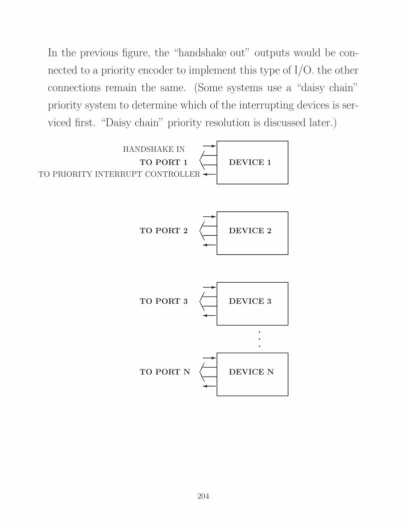
In the previous figure, the “handshake out” outputs would be con-
nected to a priority encoder to implement this type of I/O. the other
connections remain the same. (Some systems use a “daisy chain”
priority system to determine which of the interrupting devices is ser-
viced first. “Daisy chain” priority resolution is discussed later.)
TO PORT N
TO PORT 3
TO PORT 2
TO PORT 1
HANDSHAKE IN
TO PRIORITY INTERRUPT CONTROLLER ✛
✲
✁✁❆❆
✛
✲
✁✁❆❆
✛
✲
✁✁❆❆
✛
✲
✁✁❆❆
qqq
DEVICE 1
DEVICE 2
DEVICE 3
DEVICE N
204

Returning control from an interrupt
In most modern processors, interrupt return points are saved on a
“stack” in memory, in the same way as return addresses for subpro-
gram calls are saved. In fact, an interrupt can often be thought of as
a subprogram which is invoked by an external device.
The return from an interrupt is similar to a return from a subpro-
gram.
Note that the interrupt handling routine is normally responsible for
saving the state of, and restoring, any of the internal registers it uses.
If a stack is used to save the return address for interrupts, it is then
possible to allow one interrupt the interrupt handling routine of an-
other interrupt.
In many computer systems, there are several “priority levels” of in-
terrupts, each of which can be disabled, or “masked.”
There is usually one type of interrupt input which cannot be dis-
abled (a non-maskable interrupt) which has priority over all other
interrupts. This interrupt input is typically used for warning the pro-
cessor of potentially catastrophic events such as an imminent power
failure, to allow the processor to shut down in an orderly way and to
save as much information as possible.
205

Vectored interrupts
Many computers make use of “vectored interrupts.” With vectored
interrupts, it is the responsibility of the interrupting device to pro-
vide the address in main memory of the interrupt servicing routine
for that device. This means, of course, that the I/O device itself
must have sufficient “intelligence” to provide this address when re-
quested by the CPU, and also to be initially “programmed” with
this address information by the processor. Although somewhat more
complex than the simple interrupt system described earlier, vectored
interrupts provide such a significant advantage in interrupt handling
speed and ease of implementation (i.e., a separate routine for each
device) that this method is almost universally used on modern com-
puter systems.
Some processors have a number of special inputs for vectored inter-
rupts (each acting much like the simple interrupt described earlier).
Others require that the interrupting device itself provide the inter-
rupt address as part of the process of interrupting the processor.
206

Interrupts in the AVR processor
The AVR uses vectored interrupts, with fixed addresses in program
memory for the interrupt handling routines.
Interrupt vectors point to low memory; the following are the locations
of the memory vectors for some of the 23 possible interrupt events in
the ATmega168:
Address Source Event
0X000 RESET power on or reset
0X002 INT0 External interrupt request 0
0X004 INT1 External interrupt request 1
0X006 PCINT0 pin change interrupt request 0
0X008 PCINT1 pin change interrupt request 1
0X00A PCINT2 pin change interrupt request 2
0X00C WDT Watchdog timer interrupt
· ·
· ·
Interrupts are prioritized as listed; RESET has the highest priority.
Normally, the instruction at the memory location of the vector is a
jmp to the interrupt handler.
(In processors with 2K or fewer program memory words, rjmp is
sufficient.)
In fact, our earlier assembly language program used an interrupt to
begin execution — the RESET interrupt.
207

Reducing power consumption with interrupts
The previous program only actually did something interesting when
the button was pressed. The AVR processors have a “sleep” mode
in which the processor can enter a low power mode until some ex-
ternal (or internal) event occurs, and then “wake up” an continue
processing.
This kind of feature is particularly important for battery operated
devices.
The ATmega168 datasheet describes the five sleep modes in detail.
Briefly, the particular sleep mode is set by placing a value in the
Sleep Mode Control Register (SMCR). For our purposes, the Power-
down mode would be appropriate (bit pattern 0000010X) but the
simulator only understands the idle mode (0000000X).
The low order bit in SMCR is set to 1 or 0 to enable or disable sleep
mode, respectively.
The sleep instruction causes the processor to enter sleep mode, if
bit 0 of SMCR is set.
The following code can be used to set sleep mode to idle and enable
sleep mode:
ldi R16, 0b00000001 ; set sleep mode idle
out SMCR, R16 ; for power-down mode, write 00000101
208

Enabling external interrupts in the AVR
The ATmega168 datasheet describe in detail the three I/O registers
which control external interrupts. It also has a general discussion of
interrupts.
We will only consider one type of external interrupt, the pin change
interrupt. There are 16 possible pcint interrupts, labeled pcint0
to pcint15, associated with PORTE[0-7] and PORTB[0-7], respec-
tively.
There are two PCINT interrupts, PCINT0 for pcint inputs 0–7, and
PCINT1 for pcint inputs 8–15.
We are interested in using the interrupt associated with the push-
button switch connected to PINB[4], which is pcint12, and there-
fore is interrupt type PCINT1.
Two registers control external interrupts, the External Interrupt
Mask Register (EIMSK), and the External Interrupt Flag Register
(EIFR).
Only bits 0, 6, and 7 are defined for these registers. Bit 0 controls
the general external interrupt (INT0).
Bits 7 and 6 control PCINT1 and PCINT0, respectively.
Setting the appropriate bit of register EIMSK (in our case, bit 7 for
PCINT1) enables the particular pin change interrupt.
The corresponding bit in register EIFR is set when the appropriate
interrupt external condition occurs.
A pending interrupt can be cleared by writing a 1 to this bit.
209

The following code enables pin change interrupt 1 (PCINT1) and
clears any pending interrupts by writing 1 to bit 7 of the respective
registers:
sbi EIFR, 7 ; clear pin change interrupt flag 1
sbi EIMSK, 7 ; enable pin change interrupt 1
There is also a register associated with the particular pins for the
PCINT interrupts. They are the Pin Change Mask Registers (PCMSK1
and PCMSK0).
We want to enable the input connected to the switch, at PINB[4],
which is pcint12, and therefore set bit 4 of PCMSK1, leaving the
other bits unchanged.
Normally, this would be possible with the code
sbi PCMSK1, 4
Unfortunately, this register is one of the extended I/O registers, and
must be written to as a memory location.
The following code sets up its address in register pair Y, reads the
current value in PCMSK1, sets bit 4 to 1, and rewrites the value in
memory.
ldi r28, PCMSK1 ; load address of PCMSK1 in Y low
clr r29 ; load high byte of Y with 0
ld r16, Y ; read value in PCMSK1
sbr r16,0b00010000 ; allow pin change interrupt on
; PORTB pin 4
st Y, r16 ; store new PCMSK1
210

Now, the appropriate interrupt vectors must be set, as in the ta-
ble shown earlier, and interrupts enabled globally by setting the
interrupt (I) flag in the status register (SREG).
This later operation is performed with the instruction sei.
The interrupt vector table should look as follows:
.org 0
vects:
jmp RESET ; vector for reset
jmp EXT_INT0 ; vector for int0
jmp PCINT0 ; vector for pcint0
jmp PCINT1 ; vector for pcint1
jmp TIM2_COMP ; vector for timer 2 comp
The next thing necessary is to set the stack pointer to a high memory
address, since interrupts push values on the stack:
ldi r16, 0xff ; set stack pointer
out SPL, r16
ldi r16, 0x04
out SPH, r16
After this, interrupts can be enabled after the I/O ports are set up,
as in the program-controlled I/O example.
Following is the full code:
211

#include <m168def.inc>
.org 0
VECTS:
jmp RESET ; vector for reset
jmp EXT_INT0 ; vector for int0
jmp EXT_INT1 ; vector for int1
jmp PCINT_0 ; vector for pcint0
jmp BUTTON ; vector for pcint1
jmp PCINT_2 ; vector for pcint2
EXT_INT0:
EXT_INT1:
PCINT_0:
PCINT_2:
reti
RESET:
; set up pin change interrupt 1
ldi r28, PCMSK1 ; load address of PCMSK1 in Y low
clr r29 ; load high byte with 0
ld r16, Y ; read value in PCMSK1
sbr r16,0b00010000 ; allow pin change interrupt on portB pin 4
st Y, r16 ; store new PCMSK1
sbi EIMSK, 7 ; enable pin change interrupt 1
sbi EIFR, 7 ; clear pin change interrupt flag 1
ldi r16, 0xff ; set stack pointer
out SPL, r16
ldi r16, 0x04
out SPH, r16
ldi R16, 0b00100000 ; load register 16 to set portb registers
out DDRB, r16 ; set portb 5 to output, others to input
ser R16 ;
out PORTB, r16 ; set pullups (1’s) on inputs
212

sei ; enable interrupts
ldi R16, 0b00000001 ; set sleep mode
out SMCR, R16
rjmp LOOP
BUTTON:
reti
rjmp LOOP
SNOOZE:
sleep
LOOP:
sbic PINB, 4 ; skip next line if button pressed
rjmp SNOOZE ; go back to sleep if button not pressed
cbi PORTB, 5 ; set speaker input to 0
ldi R16, 128 ;
SPIN1: ; wait a few cycles
subi R16, 1
brne SPIN1
sbi PORTB, 5 ; set speaker input to 1
ldi R16, 128
SPIN2:
subi R16, 1
brne SPIN2
rjmp LOOP ; speaker buzzed 1 cycle,
; see if button still pressed
213

Direct memory access
In most desktop and larger computer systems, a great deal of input
and output occurs among several parts of the I/O system and the
processor; for example, video display, and the disk system or network
controller. It would be very inefficient to perform these operations
directly through the processor; it is much more efficient if such de-
vices, which can transfer data at a very high rate, place the data
directly into the memory, or take the data directly from the proces-
sor without direct intervention from the processor. I/O performed
in this way is usually called direct memory access, or DMA. The
controller for a device employing DMA must have the capability of
generating address signals for the memory, as well as all of the mem-
ory control signals. The processor informs the DMA controller that
data is available (or is to be placed into) a block of memory loca-
tions starting at a certain address in memory. The controller is also
informed of the length of the data block.
214

There are two possibilities for the timing of the data transfer from
the DMA controller to memory:
• The controller can cause the processor to halt if it attempts to
access data in the same bank of memory into which the controller
is writing. This is the fastest option for the I/O device, but may
cause the processor to run more slowly because the processor
may have to wait until a full block of data is transferred.
• The controller can access memory in memory cycles which are
not used by the particular bank of memory into which the DMA
controller is writing data. This approach, called “cycle stealing,”
is perhaps the most commonly used approach. (In a processor
with a cache that has a high hit rate this approach may not slow
the I/O transfer significantly).
DMA is a sensible approach for devices which have the capability of
transferring blocks of data at a very high data rate, in short bursts. It
is not worthwhile for slow devices, or for devices which do not provide
the processor with large quantities of data. Because the controller for
a DMA device is quite sophisticated, the DMA devices themselves
are usually quite sophisticated (and expensive) compared to other
types of I/O devices.
215

One problem that systems employing several DMA devices have to
address is the contention for the single system bus. There must be
some method of selecting which device controls the bus (acts as “bus
master”) at any given time. There are many ways of addressing the
“bus arbitration” problem; three techniques which are often imple-
mented in processor systems are the following (these are also often
used to determine the priorities of other events which may occur si-
multaneously, like interrupts). They rely on the use of at least two
signals (bus request and bus grant), used in a manner similar
to the two-wire handshake.
Three commonly used arbitration schemes are:
• Daisy chain arbitration
• Prioritized arbitration
• Distributed arbitration
Bus arbitration becomes extremely important when several proces-
sors share the same bus for memory. (We will look at this case in
the next chapter.)
216

Daisy chain arbitration Here, the requesting device or devices
assert the signal bus request. The bus arbiter returns the
bus grant signal, which passes through each of the devices
which can have access to the bus, as shown below. Here, the pri-
ority of a device depends solely on its position in the daisy chain.
If two or more devices request the bus at the same time, the high-
est priority device is granted the bus first, then the bus grant
signal is passed further down the chain. Generally a third sig-
nal (bus release) is used to indicate to the bus arbiter that the
first device has finished its use of the bus. Holding bus request
asserted indicates that another device wants to use the bus.
✻ ✻✲
✻
❄ ❄✛ ❄
. . .Device 1 Device nDevice 2
BusMaster
· · ·
Request
Grant Grant Grant
Priority 1 Priority 2 Priority n
217

Priority encoded arbitration Here, each device has a request line
connected to a centralized arbiter that determines which device
will be granted access to the bus. The order may be fixed by the
order of connection (priority encoded), or it may be determined
by some algorithm preloaded into the arbiter. The following
diagram shows this type of system. Note that each device has a
separate line to the bus arbiter. (The bus grant signals have
been omitted for clarity.)
❏❏
❏❏
❏❏
❍❍❍❍
��
��
Device 1
Device n
Busarbiter Device 2
...
Request
Request
Request
218

Distributed arbitration by self-selection Here, the devices them-
selves determine which of them has the highest priority. Each
device has a bus request line or lines on which it places a code
identifying itself. Each device examines the codes for all the re-
questing devices, and determines whether or not it is the highest
priority requesting device.
These arbitration schemes may also be used in conjunction with each
other. For example, a set of similar devices may be daisy chained
together, and this set may be an input to a priority encoded scheme.
There is one other arbitration scheme for serial buses — distributed
arbitration by collision detection. This is the method used by the
Ethernet, and it will be discussed later.
219

The I/O address space
Some processors map I/O devices in their own, separate, address
space; others use memory addresses as addresses of I/O ports. Both
approaches have advantages and disadvantages. The advantages of
a separate address space for I/O devices are, primarily, that the I/O
operations would then be performed by separate I/O instructions,
and that all the memory address space could be dedicated to memory.
Typically, however, I/O is only a small fraction of the operations
performed by a computer system; generally less than 1 percent of all
instructions are I/O instructions in a program. It may not be worth-
while to support such infrequent operations with a rich instruction
set, so I/O instructions are often rather restricted.
In processors with memory mapped I/O, any of the instructions
which references memory directly can also be used to reference I/O
ports, including instructions which modify the contents of the I/O
port (e.g., arithmetic instructions.)
220

Some problems can arise with memory mapped I/O in systems which
use cache memory or virtual memory. If a processor uses a virtual
memory mapping, and the I/O ports are allowed to be in a virtual
address space, the mapping to the physical device may not be con-
sistent if there is a context switch or even if a page is replaced.
If physical addressing is used, mapping across page boundaries may
be problematic.
In many operating systems, I/O devices are directly addressable only
by the operating system, and are assigned to physical memory loca-
tions which are not mapped by the virtual memory system.
If the memory locations corresponding to I/O devices are cached,
then the value in cache may not be consistent with the new value
loaded in memory. Generally, either there is some method for in-
validating cache that may be mapped to I/O addresses, or the I/O
addresses are not cached at all. We will look at the general prob-
lem of maintaining cache in a consistent state (the cache coherency
problem) in more detail when we discuss multi-processor systems.
221

In the “real world” ...
Although we have been discussing fairly complex processors like the
MIPS, the largest market for microprocessors is still for small, simple
processors much like the early microprocessors. In fact, there is still
a large market for 4-bit and 8-bit processors.
These devices are used as controllers for other products. A large part
of their function is often some kind of I/O, from simple switch inputs
to complex signal processing.
One function of such processors is as I/O processors for more so-
phisticated computers. The following diagram shows the sales of
controllers of various types:
.2
6
8
4
10
12
91 93 94 969592
4.9 5.2
6.6
8.2
9.9
11.7
4-bit
8-bit
16/32-bit
DSP
SALES(billions, US)
The projected microcontroller sales for 2001 is 9.8 billion; for 2002,
222

9.6 billion; for 2003, 12.0 billion; for 2004, 13.0 billion; for 2005, 14
billion. (SIA projection.)
For DSP devices, it is 4.9 billion in 2002, 6.5 billion in 2003, 8.4
billion in 2004, and 9.4 billion in 2005.
223

Magnetic disks
A magnetic disk drive consists of a set of very flat disks, called plat-
ters, coated on both sides with a material which can be magnetized
or demagnetized.
The magnetic state can be read or written by small magnetic heads
located on mechanical arms which can move in and out over the
surfaces of the disks, very close to but not actually touching, the
surfaces.
224

Each platter containing a number of tracks, and each track containing
a set of sectors.
Platters
Tracks
Sectors
Total storage is
(no. of platters) × (no. of tracks/platter) × (no. of sectors/track)
Typically, disks are formatted and bad sectors are noted in a table
stored in the controller.
225

Disks spin at speeds of 4200 RPM to 15,000 RPM. Typical speeds for
PC desktops are 7200 RPM and 10,000 RPM. Laptop disks usually
spin at 4200 or 5400 RPM.
“Disk speed” is usually characterized by several parameters:
average seek time, which is the average required for the read/write
head to be positioned over the correct track, typically about 8ms.
rotational latency which is the average time for the appropriate
sector to rotate to a point under the head, (4.17 ms for a 7200
RPM disk) and
transfer rate, this is about 5Mbytes/second for an early IDE drive.
(33 – 133 MB/s for an ATA drive, and 150 – 300 MB/s for a
SATA drive.) Typically, sustained rates are less than half the
maximum rates.
controller overhead also contributes some delay; typically ≤ 1 ms.
Assuming a sustained data transfer rate of 50MB/s, the time required
to transfer a 1 Kbyte block is
8ms. + 4.17ms. + 0.02 ms. + 1ms. = 13.2 ms.
To transfer a 1 Mbyte block in the same system, the time required is
8ms. + 4.17ms. + 20 ms. + 1ms. = 33 ms.
Note that for small blocks, most of the time is spent finding the data
to be transferred. This time is the latency of the disk.
226

Latency can be reduced in several ways in modern disk systems.
• The disks have built-in memory buffers which store data to be
written, and which also can contain data for several reads at the
same time. (In this case, the reads and writes are not necessarily
performed in the order in which they are received.)
• The controller can optimize the seek path (overall seek time) for
a set of reads, and thereby increase throughput.
• The system may contain redundant information, and the sector,
or disk, with the shortest access can supply the data.
In fact, systems are often built with large, redundant disk arrays for
several reasons. Typically, security against disk failure and increased
read speed are the main reasons for such systems.
Large disks are now so inexpensive that the Department now uses
large disk arrays as backup storage devices, replacing the slower and
more cumbersome tape drives. Presently, the department maintains
servers with several terabytes of redundant disk.
227

Disk arrays — RAID
Disk performance and/or reliability of a disk system can be increased
using an array of disks, possibly with redundancy — a Redundant
Array of Independent Disks, or RAID.
Raid systems use two techniques to improve performance and relia-
bility — striping and redundancy.
Striping simply allocates successive disk blocks to different disks.
This can increase both read and write performance, since the opera-
tions are performed in parallel over several disks.
RAIDs use two different forms of redundancy — replication (mirror-
ing) and parity (error correction).
A system with replication simply writes a copy of data on a second
disk — the mirror. This increases the performance of read opera-
tions, since the data can be read from both disks in parallel. Write
performance is not improved, however.
Also, failure of one disk will not cause the system to fail.
Parity is used to provide the ability to recover data if one disk fails.
This is the way data is most often replicated over several disks.
In the following example, if the parity is even and there is a single bit
missing, then the missing bit can be determined. Here, the missing
bit must be a 1 to maintain even parity.
mn1mn0mn1mn1
mn1mn0 mn1mnX
✻❄ mnparity bit
mn1
mn1
228

There are several defined levels of RAID, as follows:
RAID 0 has no redundancy, it simply stripes data over the disks
in the array.
RAID 1 uses mirroring. This is full redundancy, and provides tol-
erance to failure and increased read performance.
RAID 2 uses error correction alone. This type of RAID is no longer
used.
RAID 3 uses bit-interleaved parity. Here each access requires data
from all the disks. The array can recover from the failure of one
disk. Read performance increases because of the parallel access.
RAID 4 uses block-interleaved parity. This can allow small reads
to access fewer disks (e.g., a single block can be read from one
disk). The parity disk is read and rewritten for all writes.
RAID 5 uses distributed block-interleaved parity. this is similar to
RAID 4, but the parity blocks are distributed over all disks. This
can increase write performance as well as read performance. (All
parity writes do not access one only disk.)
Some systems support two RAID levels. The most common example
of this is RAID 0+1. This is a striped, mirrored disk array. It
provides redundancy and parallelism for both reads and writes.
229

Failure tolerance
RAID levels above 0 provide tolerance to single disk failure. Systems
can actually rebuild a file system after the failure of a single disk.
Multiple disk failure generally results in the corruption of the whole
file system.
RAID level 0 actually makes the system more vulnerable to disk
failure — failure of a single disk can destroy the data in the whole
array.
For example, assume a disk has a failure rate of 1%. The probability
of a single failure in a 2 disk system is
0.01 + (1.− 0.01)× 0.01 ≈ 0.02 = 2%
Consider a RAID 3, 4, or 5 system with 4 disks. Here, 2 disks must
fail at the same time for a system failure.
Consider a 4 disk system with the same failure rate. The probability
of exactly two disks failing (and two not failing) is
(1− 0.01)2 × (0.01)2 ≈ 0.0001 = 0.01%
230

Networking — the Ethernet
Originally, the physical medium for the Ethernet was a single coaxial
cable with a maximum length of about 500 M. and a maximum of
100 connections.
It was basically a single, high speed (at the time) serial bus network.
It had a particularly simple distributed control mechanism, as well
as ways to extend the network (repeaters, bridges, routers, etc.)
We will describe the original form of the Ethernet, and its modern
switched counterpart.
Hoststation
Hoststation
Hoststation
Coax cable
Transcevertap
Terminator
In the original Ethernet, every host station (system connected to the
network) was connected through a transceiver cable.
Only one host should talk at any given time, and the Ethernet has a
simple, distributed, mechanism for determining which host can access
the bus.
231

The network used a variable length packet, transmitted serially at
the rate of 10 Mbits/second, with the following format:
46 − 1500 bytes48 48 16 3264 bits
Dest. Source Type DataAddr. Addr. Field Field CRCPreamble
The preamble is a synchronization pattern containing alternating 0’s
and 1’s, ending with 2 consecutive 1’s:
101010101010...101011
The destination address is the address of the station(s) to which
the packet is being transmitted. Addresses beginning with 0 are
individual addresses, those beginning with 1 are multicast (group)
addresses, and address 1111...111 is the broadcast address.
The source address is the unique address of the station transmitting
the message.
The type field identifies the high-level protocol associated with the
message. It determines how the data will be interpreted.
The CRC is a polynomial evaluated using each bit in the message,
and is used to determine transmission errors, for data integrity.
The minimum spacing between packets (interpacket delay) is 9.6 µs.
From the above diagram, the minimum and maximum packet sizes
are 72 bytes and 1526 bytes, requiring 57.6 µs. and 1220.8 µs.,
respectively.
232

One of the more interesting features of the Ethernet protocol is the
way in which a station gets access to the bus.
Each station listens to the bus, and does not attempt to transmit
while another station is transmitting, or in the interpacket delay
period. In this situation, the station is said to be deferring.
A station may transmit if it is not deferring. While a station trans-
mits, it also listens to the bus. If it detects an inconsistency between
the transmitted and received data (a collision, caused by another
station transmitting) then the station aborts transmission, and sends
4-6 bytes of junk (a jam) to ensure every other station transmitting
also detects the collision.
Each transmitting station then waits a random time interval before
attempting to retransmit. On consecutive collisions, the size of the
random interval is doubled, to a maximum of 10 collisions. The base
interval is 512 bit times (51.2 µs.)
This arbitration mechanism is fair, an not rely on any central arbiter,
and is simple to implement.
While it may seem inefficient, usually there are relatively few colli-
sions, even in a fairly highly loaded network. The average number of
collisions is actually quite small.
Wireless networks currently use a quite similar mechanism for deter-
mining which node can transmit a packet. (Normally, only one node
can transmit at a time, and control is distributed.)
233

Current ethernet systems
The modern variant of the Ethernet is quite different (but the same
protocols apply).
In the present system, individual stations are connected to a switch,
using an 8-conductor wire (Cat-5 wire, but only 4 wires are actually
used) which allows bidirectional traffic from the station to the switch
at 100 Mbits/s in either direction.
A more recent variant uses a similar arrangement, with Cat-6 wire,
and can achieve 1 Gbit/second.
stationHost
stationHost
stationHost
Switch
Cat−5 wire
A great advantage of this configuration is that there is only one
station on each link, so other stations cannot “eavesdrop” on the
network communications.
Another advantage of switches is that several pairs of stations can
communicate with each other simultaneously, reducing collisions dra-
matically.
234

The maximum length of a single link is 100 m., and switches are
often linked by fibre optical cable.
The following pictures show the network in the Department:
The first shows the cable plant (where all the Cat-5 wires are con-
nected to the switches).
The second shows the switches connecting the Department to the
campus network. It is an optical fiber network operating at 10 Gbit/s.
The optical fiber cables are orange.
The third shows the actual switches used for the internal network.
Note the orange optical fibre connection to each switch.
235

236

In the following, note the orange optical fibre cable.
237

238

In the previous picture, there were 8 sets of high-speed switches,
each with 24 1 Gbit/s. ports, and 1 fibre optical port at 10 Gbit/s.
Each switch is interconnected to the others by a backplane connector
which can transfer data at 2 Gbits/s.
The 10 Gbit/s. ports are connected to the departmental servers
which collectively provide several Tera-bytes of redundant (raid) disk
storage for departmental use.
239

Multiprocessor systems
In order to perform computation faster, there are two basic strategies:
• Increase the speed of individual computations.
• Increase the number of operations performed in parallel.
At present, high-end microprocessors are manufactured using aggres-
sive technologies, so there is relatively little opportunity to take the
first strategy, beyond the general trend (Moore’s law).
There are a number of ways to pursue the second strategy:
• Increase the parallelism within a single processor, using multiple
parallel pipelines and fast access to memory. (e.g., the Cray
computers).
• Use multiple commercial processors, each with its own memory
resources, interconnected by some network topology.
• Use multiple commercial microprocessors “in the same box” —
sharing memory and other resources.
The first of these approaches was successful for several decades, but
the low cost per unit of commercial microprocessors is so attractive
that the microprocessor based systems have the potential to provide
very high performance computing at relatively low cost.
240

Multiprocessor systems
A multiprocessor system might look as follows:
InterconnectNetwork
Processors Processors
The interconnect network can be switches, single or multiple serial
links, or any other network topology.
Here, each processor has its own memory, but may be able to access
memory from other processors as well.
Also nearby processors may communicate faster than processors that
are further away.
241

An alternate system, (a shared memory multiprocessor system) where
processors share a large common memory, could look as follows:
InterconnectNetwork
MemoryProcessors
The interconnect network can be switches, single or multiple buses,
or any other topology.
The single bus variant of this type of system is now quite common.
Many manufacturers provide quad, or higher, core processors, and
multiprocessing is supported by many different operating systems.
242

A single bus shared memory multiprocessor system:
tag
tag
tag
tag
GlobalbusProcessors Cache
busseslocal
Memory
Shared
Note that here each processor has its own cache. Virtually all current
high performance microprocessors have a reasonable amount of high
speed cache implemented on chip.
In a shared memory system, this is particularly important to reduce
contention for memory access.
243

The cache, while important for reducing memory contention, must
behave somewhat differently than the cache in a single processor
system.
Recall that a cache had four components:
• high speed storage
• an address mapping mechanism from main memory to cache
• a replacement policy for data which is not found in cache
• a mechanism for handling writes to memory.
Reviewing the design characteristics of a single processor cache, we
found that performance increased with:
• larger cache size
• larger line (block) size
• larger set size — associativity, mapping policy
• “higher information” line replacement policy (miss ratio for LRU
< FIFO < random)
• lower frequency cache-to-memory write policy (write-back better
than write-through)
244

Multiprocessor Cache Coherency
In shared memory multiprocessor systems, cache coherency — the
fact that several processors can write to the same memory location,
which may also be in the cache of one or more other processors —
becomes an issue.
This makes both the design and simulation of multiprocessor caches
more difficult.
Cache coherency solutions
Data and instructions can be classified as
read-only or writable,
and shared or unshared.
It is the shared, writable data which allows the cache to become
incoherent.
There are two possible solutions:
1. Don’t cache shared, writable data.
Cache coherency is not an issue then, but performance can suffer
drastically because of uncached reads and writes of shared data.
This approach can be used with either hardware or software.
245

2. Cache shared, writable data and use hardware to maintain cache
coherence.
Again, there are two possibilities for writing data:
(a) data write-through (or buffered write-through)
(This may require many bus operations.)
(b) some variant of write-back
Here, there are two more possibilities:
i. write invalidate— the cache associated with a processor
can invalidate entries written by other processors, or
ii. write update — the cache can update its value with that
written in the other cache.
Most commercial bus-based multi-processors use a write-back
cache with write invalidate. This generally reduces the bus traf-
fic.
Note that to invalidate a cache entry on a write, the cache only
needs to receive the address from the bus.
To update, the cache also needs the data from the other cache,
as well.
246

One example of an invalidating policy is the write-once policy —
a cache writes data back to memory one time (the first write) and
when the line is flushed. On the first write, other caches in the
system holding this data mark their entries invalid.
A cache line can have 4 states:
invalid — cache data is not correct
clean — memory is up-to-date, data may be in other caches
reserved — memory is up-to-date; no other caches have this data
dirty — memory is incorrect; no other cache holds this data
As an exercise, try to determine what happens in the caches for all
possible transitions.
This is an example of a snoopy protocol — the cache obtains its
state information by listening to, or “snooping” the bus.
247

The Intel Pentium class processors use a similar cache protocol called
theMESI protocol. Most other single-chip multiprocessors use this,
or a very similar protocol, as well.
The MESI protocol has 4 states:
modified — the cache line has been modified, and is available only
in this cache (dirty)
exclusive — no other caches have this line, and it is consistent
with memory (reserved)
shared — line may also be in other caches, memory is up-to-date
(clean)
invalid — cache line is not correct (invalid)
M E S I
Cache line valid? Yes Yes Yes No
Memory is Stale Valid Valid ?
Multiple cache copies? No No Maybe Maybe
What happens for read and write hits and misses?
248

Read hit
For a read hit, the processor takes data directly from the local cache
line, as long as the line is valid. (If it is not valid, it is a cache miss,
anyway.)
Read miss
Here, there are several possibilities:
• If no other cache has the line, the data is taken from memory
and marked exclusive.
• If one or more caches have a clean copy of this line, (either in
states exclusive or shared) they should signal the cache, and
each cache should mark its copy as shared.
• If a cache has a modified copy of this line, it signals the cache
to retry, writes its copy to memory immediately, and marks its
cached copy as shared. (The requesting cache will then read the
data from memory, and have it marked as shared.)
249

Write hit
The processor marks the line in cache as modified. If the line was
already in state modified or exclusive, then that cache has the only
copy of the data, and nothing else need be done. If the line was in
state shared, then the other caches should mark their copies invalid.
(A bus transaction is required).
Write miss
The processor first reads the line from memory, then writes the word
to the cache, marks the line as modified, and performs a bus transac-
tion so that if any other cache has the line in the shared or exclusive
state it can be marked invalid.
If, on the initial read, another cache has the line in the modified
state, that cache marks its own copy invalid, suspends the initiating
read, and immediately writes its value to memory. The suspended
read resumes, getting the correct value from memory. The word can
then be written to this cache line, and marked as modified.
250

False sharing
One type of problem possible in multiprocessor cache systems using
a write-invalidate protocol is “false sharing.”
This occurs with line sizes greater than a single word, when one pro-
cessor writes to a line that is stored in the cache of another processor.
Even if the processors do not share a variable, the fact that an entry
in the shared line has changed forced the caches to treat the line as
shared.
It is instructive to consider the following example (assume a line size
of 4 32 bit words, and that all caches initially contain clean, valid
data):
Step Processor Action address
1 P1 write 100
2 P2 write 104
3 P1 read 100
4 P2 read 104
Note that addresses 100 and 104 are in the same cache line (the line
is 4 words or 16 bytes, and the addresses are in bytes).
Consider the MESI protocol, and determine what happens at each
step.
251

Example — a simple multiprocessor calculation
Suppose we want to sum 16 million numbers on 16 processors in a
single bus multiprocessor system.
The first step is to split the set of numbers into subsets of the same
size. Since there is a single, common memory for this machine, there
is no need to partition the data; we just give different starting ad-
dresses in the array to each processor. Pn is the number of the
processor, between 0 and 15.
All processors start the program by running a loop that sums their
subset of numbers:
tmp = 0;
for (i = 1000000 * Pn; i < 1000000 * (Pn+1);
i = i + 1) {
tmp = tmp + A[i]; /* sum the assigned areas*/
}
sum[Pn] = tmp
This loop uses load instructions to bring the correct subset of num-
bers to the caches of each processor from the common main memory.
Each processor must have its own version of the loop counter variable
i, so it must be a “private” variable. Similarly for the partial sum,
tmp. The array sum[Pn] is a global array of partial sums, one from
each processor.
252

The next step is to add these many partial sums, using “divide and
conquer.” Half of the processors add pairs of partial sums, then a
quarter add pairs of the new partial sums, and so on until we have
the single, final sum.
In this example, the two processors must synchronize before the
“consumer” processor tries to read the result written to memory
by the “producer” processor; otherwise, the consumer may read the
old value of the data. Following is the code (half is private also):
half = 16; /* 16 processors in multiprocessor*/
repeat
synch(); /* wait for partial sum completion*/
if (half%2 !=0 && Pn == 0)
sum[0] = sum[0] + sum[half-1];
half = half/2; /* dividing line on who sums */
if (Pn < half) sum[Pn] = sum[Pn] + sum[Pn+half];
until (half == 1); /* exit with final sum in Sum[0]*/
Note that this program used a “barrier synchronization” primitive,
synch(); processors wait at the “barrier” until every processor has
reached it, then they proceed.
This function can be implemented either in software with the lock
synchronization primitive, described shortly, or with special hardware
(e.g., combining each processor “ready” signal into a single global
signal that all processors can test.)
253

Does the parallelization actually speed up this computation?
It is instructive to calculate the time required for this calculation,
assuming that none of the data values have been read previously
(and are not in the caches for each processor).
In this case, each memory location is accessed exactly once, and
access to memory determines the speed of each processor. Assume
that a single data word is taken from memory on each bus cycle. The
overall calculation requires 16 million memory bus cycles, plus the
additional cycles required to sum the 16 partial values.
Note that if the computation has been done by a single processor,
the time required would have been only the time to access the 16
million data elements.
Of course, if each of the processors already had the requisite 1 million
data elements in their local memory (cache), then the speedup would
be achieved.
It is instructive to consider what would be the execution time for
other scenarios; for example, if the line size for each cache were four
words, or if each cache could hold,say, 2 million words, and the data
had been read earlier and was already in the cache.
254

Synchronization Using Cache Coherency
A key requirement of any multiprocessor system (or, in fact, any pro-
cessor system that allows multiple processes to proceed concurrently)
is to be able to coordinate processes that are working on a common
task.
Typically, a programmer will use lock variables (or semaphores) to
coordinate or synchronize the processes.
Arbitration is relatively easy for single-bus multiprocessors, since the
bus is the only path to memory: the processor that gets the bus
locks out all other processors from memory. If the processor and bus
provide an atomic test-and-set operation, programmers can create
locks with the proper semantics. Here the term atomic means indi-
visible, so the processor can both read a location and set it to the
locked value in the same bus operation, preventing any other proces-
sor or I/O device from reading or writing memory until the operation
completes.
The following diagram shows a typical procedure for locking a vari-
able using a test-and-set instruction. Assume that 0 means unlocked
(“go”) and 1 means locked (“stop”). A processor first reads the lock
variable to test its state. It then keeps reading and testing until the
value indicates that the lock is unlocked.
255

The processor then races against all other processors that were simi-
larly spin waiting to see who can lock the variable first. All processors
use a test-and-set instruction that reads the old value and stores a
1 (“locked”) into the lock variable. The single winner will see the 0
(“unlocked”), and the losers will see a 1 that was placed there by the
winner. (The losers will continue to write the variable with the locked
value of 1, but that doesn’t change its value.) The winning processor
then executes the code that updates the shared data. When the win-
ner exits, it stores a 0 (“unlocked”) into the lock variable, thereby
starting the race all over again.
The term usually used to describe the code segment between the lock
and the unlock is a “critical section.”
256

❄
❄
✛
❄
❄
✛
❄❄
❄
❄
✟✟✟✟✟✟❍❍❍❍❍❍✟✟✟✟✟✟❍❍
❍❍❍❍
✟✟✟✟✟✟❍❍❍❍❍❍✟✟✟✟✟✟❍❍
❍❍❍❍
Load lockvariable S
Unlocked?
Try to lock variableusing test-and-set
(set S = 1)
S = 0
Yes
No
Yes
No
Access shared
Unlock(Set S = 0)
(S = 0)Succeed?
Compete forlock
resourceCriticalsection
257

Let us see how this spin lock scheme works with bus-based cache
coherency.
One advantage of this scheme is that it allows processors to spin wait
on a local copy of the lock in their caches. This dramatically reduces
the amount of bus traffic; The following table shows the bus and
cache operations for multiple processors trying to lock a variable.
Once the processor with the lock stores a 0 into the lock, all other
caches see that store and invalidate their copy of the lock variable.
Then they try to get the new value of 0 for the lock. (With write
update cache coherency, the caches would update their copy rather
than first invalidate and then load from memory.) This new value
starts the race to see who can set the lock first. The winner gets the
bus and stores a 1 into the lock; the other caches replace their copy
of the lock variable containing 0 with a 1.
They read that the variable is already locked and must return to
testing and spinning.
Because of the communication traffic generated when the lock is
released, this scheme has difficulty scaling up to many processors.
258

Step P0 P1 P2 Bus Activity
1 Has lock Spin (test if
lock=0)
Spin None
2 Set lock=0
and 0 sent
over bus
Spin Spin Write-
invalidate of
lock variable
from P0
3 Cache miss Cache miss Bus decides
to service P2
cache miss
4 (Waits while
bus busy)
Lock = 0 Cache miss
for P2 satis-
fied
5 Lock = 0 Swap: reads
lock and sets
to 1
Cache miss
for P2 satis-
fied
6 Swap: reads
lock and sets
to 1
Value from
swap =0
and 1 sent
over bus
Write-
invalidate of
lock variable
from P2
7 Value from
swap = 1
and 1 sent
over bus
Owns the
lock, so
can update
shared data
Write-
invalidate of
lock variable
from P1
8 Spins None
259

Multiprocessing without shared memory — networked
processors
InterconnectNetwork
Processors Processors
Here the interconnect can be any desired interconnect topology.
260

The following diagrams show some useful network topologies. Typi-
cally, a topology is chosen which maps onto features of the program
or data structures.
1D mesh
2D mesh
Ring
2D torus
3D grid
Tree
Some parameters used to characterize network graphs include:
bisection bandwidth — the minimum number of links which must
be removed to partition the graph
network diameter — the maximum of the “minimum distance
between two nodes”
261

Hypercube
Butterfly
In the following, the layout area is (eventually) dominated by the interconnections:
262

Let us assume a simple network; for example, a single high-speed
Ethernet connection to a switched hub.
(This is a common approach for achieving parallelism in Linux sys-
tems. Parallel systems like this are often called “Beowulf clusters.”)
Processor Processor Processor Processor
Processor Processor Processor Processor
Switch
Note that in this configuration, any two processors can communicate
with each other, simultaneously. Collisions (blocking) only occur
when two processors attempt to send messages to the same processor.
(This is equivalent to a permutation network, if a single switch is
sufficient.)
263

Parallel Program (Message Passing)
Let us reexamine our summing example again for a network-connected
multiprocessor with 16 processors each with a private memory.
Since this computer has multiple address spaces, the first step is dis-
tributing the 16 subsets to each of the local memories. The processor
containing the 16,000,000 numbers sends the subsets to each of the
16 processor-memory nodes.
Let Pn represent the number of the execution unit, send(x,y,len)
be a routine that sends over the interconnection network to execution
unit number x the list y of length len words, and receive(x) be
a function that accepts this list from the network for this execution
unit:
procno = 16; /* 16 processors */
for (Pn = 0; Pn < procno; Pn = Pn + 1
send(Pn, A(Pn*1000000), 1000000);
264

The next step is to get the sum of each subset. This step is simply
a loop that every execution unit follows; read a word from local
memory and add it to a local variable:
receive(A1);
sum = 0;
for (i = 0; i<1000000; i = i + 1)
sum = sum + A1[i]; /* sum the local arrays */
Again, the final step is adding these 16 partial sums. Now, each
partial sum is located in a different execution unit. Hence, we must
use the interconnection network to send partial sums to accumulate
the final sum.
Rather than sending all the partial sums to a single processor, which
would result in sequentially adding the partial sums, we again apply
“divide and conquer.” First, half of the execution units send their
partial sums to the other half of the execution units, where two partial
sums are added together. Then one quarter of the execution units
(half of the half) send this new partial sum to the other quarter of the
execution units (the remaining half of the half) for the next round of
sums.
265

This halving, sending, and receiving continues until there is a single
sum of all numbers.
limit = 16;
half = 16; /* 16 processors */
repeat
half = (half+1)/2; /* send vs. receive dividing line*/
if (Pn >= half && Pn < limit) send(Pn - half, sum, 1);
receive(tmp);
if (Pn < (limit/2-1)) sum = sum + tmp;
limit = half; /* upper limit of senders */
until (half == 1); /* exit with final sum */
This code divides all processors into senders or receivers and each
receiving processor gets only one message, so we can presume that a
receiving processor will stall until it receives a message. Thus, send
and receive can be used as primitives for synchronization as well as
for communication, as the processors are aware of the transmission
of data.
266

How much does parallel processing help?
In the previous course, we met Amdahl’s Law, which stated that, for
a given program and data set, the total amount of speedup of the
program is limited by the fraction of the program that is serial in
nature.
If P is the fraction of a program that can be parallelized, and the
serial (non-parallelizable) fraction of the code is 1−P then the total
time taken by the parallel system is (1 − P ) + P/N . The speedup
S(N) with N processors is therefore
S(N) =1
(1− P ) + P/N
As N becomes large, this approaches 1/(1− P ).
So, for a fixed problem size, the serial component of a program limits
the speedup.
Of course, if the program has no serial component, then this is not
a problem. Such programs are often called “trivially parallelizable”,
but many interesting problems are not of this type.
Although this is a pessimistic result, in reality it may be possible to
do better, just not for a fixed problem size.
267

Gustafson’s law
One of the advantages of increasing the amount of computation avail-
able for a problem is that problems of a larger size can be attempted.
So, rather than keeping the problem size fixed, suppose we can for-
mulate the problem to try to use parallelism to solve a larger problem
in the same amount of time. (Gustafson called this scaled speedup).
The idea here is that, for certain problems, the serial part use a nearly
constant amount of time, while the parallel part can scale with the
number of processors.
Assume that a problem has a serial component s and a parallel com-
ponent p.
So, if we have N processors, the time to complete the equivalent
computation on a single processor is s +Np.
The speedup S(N) is:
(single processor time)/(N processor time) or (s +Np)/(s + p)
Letting α be the sequential fraction of the parallel execution time,
α = s/(s + p)
then S(N) = α +N(1− α)
If α is small, then S(N) ≈ N .
For problems fitting this model, the speedup is really the best one
can hope from applying N processors to a problem.
268

So, we have two models for analyzing the potential speedup for par-
allel computation.
They differ in the way they determine speedup.
Let us think of a simple example to show the difference between the
two:
Consider booting a computer system. It may be possible to reduce
the time required somewhat by running several processes simultane-
ously, but the serial nature will pose a lower limit on the amount of
time required. (Amdhal’s Law).
Gustafson’s Law would say that, in the same time that is required
to boot the processor, more facilities could be made available; for
example, initiating more advanced window managers, or bringing up
peripheral devices.
A common explanation of the difference is:
Suppose a car is traveling between two cities 90 km. apart. If the
car travels at 60 km/h for the first hour, then it can never average
100 km/h between the two cities. (Amdhal’s Law.)
Suppose a car is traveling at 60 km. per hour for the first hour. If it
is then driven consistently at a speed greater than 100 km/h, it will
eventually average 100 km/h. (Gustafson’s Law.)
269