allen cell types database - help

JUNE 2016 v.3 alleninstitute.org

Electrophysiology brain-map.org

page 1 of 15

Allen Cell Types Database

TECHNICAL WHITE PAPER: ELECTROPHYSIOLOGY OVERVIEW This Technical White Paper describes the reagent preparation, specimen processing, selection of target regions for experimentation, preparation of tissue for slice electrophysiology, electrophysiological recordings, electrophysiology stimuli strategy and details, and electrophysiology data curation and quality evaluation (both at a cell level and a sweep level). Slices were prepared from P45 to P70 mice (either an interneuron or layer specific Cre driver line crossed to an Ai14 tdTomato reporter line). Slices (350 µm) were sectioned using a vibrating microtome: each slice was imaged to aid in brain region identification and registration to the Allen Mouse Common Coordinate Framework. For more information on the CCF, see the whitepaper located in the Documentation tab. Whole cell current clamp recordings were made from identified, tdTomato-positive neurons. Stimulation waveforms were designed to: 1) interrogate intrinsic membrane properties that contribute to the input/output function of neurons, 2) understand aspects of neural response properties in vivo, and 3) construct and test computational models of varying complexity emulating the neural response to stereotyped stimuli at the soma. Stimulus sets were divided into 2 groups: a rigid ‘Core 1’ sequence designed to establish baseline properties that is applied to every neuron, and a more flexible ‘Core 2’ sequence that can be tailored to each Cre line and is influenced by close feedback from modelers and in vivo recordings. Electrophysiology data were reported with metadata detailing experimental conditions such as electrode resistance, tight seal resistance, and series resistance, as well as more granular details such as bath temperature and amplifier settings on a sweep by sweep basis. Data were curated based on cell-wide and sweep-based Quality Control (QC) criteria. REAGENT PREPARATION Three variations of Artificial Cerebrospinal Fluid (ACSF) were made fresh twice a week. ACSF.I and ACSF.IV were used for transcardial perfusion and tissue incubation. ACSF.III was used for bathing the tissue during the electrophysiological recording session. ACSF.I ACSF.I was used for transcardial perfusion and has the following composition: 0.5 mM calcium chloride (dehydrate), 25 mM D-glucose, 98 mM hydrochloric acid, 20 mM HEPES, 10 mM magnesium sulfate, 1.25 mM sodium phosphate monobasic monohydrate, 3 mM myoinositol, 12 mM N-acetyl-L-cysteine, 98 mM N-methyl-d-glucamine (NMDG), 2.5 mM potassium chloride, 25 mM sodium bicarbonate, 5 mM sodium L-ascorbate, 3 mM sodium pyruvate, 0.01 mM taurine, and 2 mM thiourea. Prior to use, the solution was equilibrated with 95% O2, 5% CO2. Osmolality was verified to be between 295-305 mOsm/kg. pH was adjusted to 7.3 using HCl. For increased neuronal survival, ACSF.I was modified to contain a decreased sodium concentration (substituted with NMDG, Zhao et al., 2011) and elevated magnesium concentrations as well as N-acetyl-L-cysteine and sodium ascorbate to reduce oxidative damage. ACSF.III ACSF.III was used for bathing tissue during the electrophysiological recording session and contains 2 mM calcium chloride (dehydrate), 12.5 mM D-glucose, 1 mM kynurenic acid, 1 mM magnesium sulfate, 1.25 mM

http://help.brain-map.org/display/celltypes/Documentation

TECHNICAL WHITE PAPER



page 2 of 15

sodium phosphate monobasic monohydrate, 0.1 mM picrotoxin, 2.5 mM potassium chloride, 26 mM sodium bicarbonate, and 126 mM sodium chloride. Prior to use, the solution was equilibrated with 95% O2, 5% CO2. Osmolality was verified to be between 295-305 mOsm/kg. pH was adjusted to 7.3 using HCl or NaOH. ACSF.IV ACSF.IV was used for tissue maintenance prior to recording and contains 2 mM calcium chloride (dehydrate), 25 mM D-glucose, 20 mM HEPES, 2 mM magnesium sulfate, 1.25 mM sodium phosphate monobasic monohydrate, 3 mM myo inositol, 12.3 mM N-acetyl-L-cysteine, 2.5 mM potassium chloride, 25 mM sodium bicarbonate, 97 mM sodium chloride, 5 mM sodium L-ascorbate, 3 mM sodium pyruvate, 0.01 mM taurine, and 2 mM thiourea. Prior to use, the solution was equilibrated with 95% O2, 5% CO2. Osmolality was verified to be between 295-305 mOsm/kg. pH was adjusted to 7.3 using NaOH. Internal Solution with Biocytin For electrophysiological recording and cell filling, an internal solution with biocytin was prepared, containing 126 mM potassium gluconate, 10.0 mM HEPES, 0.3 mM ethylene glycol-bis (2-aminoethylether)-N,N,N’,N’-tetraacetic acid, 4 mM potassium chloride, 0.3 mM guanosine 5’-triphosphate sodium salt hydrate, 10 mM phosphocreatine disodium salt hydrate, 4 mM adenosine 5′-triphosphate magnesium salt, and 0.5% biocytin (Sigma B4261). Osmolality was verified to be between 285-295 mOsm/kg. Internal solution batches were used within 60 days. pH was adjusted to 7.3 using KOH. SPECIMEN PROCESSING Mice (male and female) between the ages of P45-P70 were anesthetized with 5% isoflurane and intracardially perfused with 50 ml of ice cold oxygenated slicing artificial cerebral spinal fluid (ACSF.I) at a flow rate of 9 ml per minute until the liver appeared clear or the 50 ml was finished. The brain was then rapidly dissected and mounted for coronal slice preparation (rostral end at base) on the chuck of a Compresstome VF-300 vibrating microtome (Precisionary Instruments). Using a custom designed photodocumentation configuration (Mako G125B PoE camera with custom integrated software), a blockface image was acquired before each section was sliced in the coronal plane, at a section thickness of 350 µm (Figure 1). The 350 µm thick slice was then captured and hemisected along the midline. Tissue slices were then recovered using one of two protocols.

1) Data acquired prior to 2016. Slices were transferred to oxygenated and warmed (34ºC) incubation solution (ACSF.IV) for 10 minutes. Slices were incubated for at least one hour in specimen holders fitted with mesh bottoms (Part # 36157-1, Ted Pella, Inc.) and immersed in ACSF.IV that was continuously bubbled with a gas mix of 95% O2, 5% CO2. The temperature of the bathing ACSF gradually cooled from 34ºC to room temperature over the course of the one hour incubation time.

2) Data acquired during/after 2016. Slices were transferred to oxygenated and warmed (34ºC) slicing solution (ACSF.I) for 10 minutes. Slices were then transferred to room temperature incubation solution (ACSF.IV) bubbled with a gas mix of 95% O2, 5% CO2. Slices recovered for at least one hour before the beginning of the recording session. For both the 10 minute and 1+ hour recovery incubations, slices were held in BSK12 Brain Slice Keepers (Scientific Systems Design Inc.).

Using a blind pilot study on slice preparation methods, the second protocol was shown to provide slices with a greater number of patchable neurons and higher success obtaining intact morphology following electrophysiology recording. Electrophysiology features extracted from data acquired using the modified preparation do not differ significantly from previous data. SELECTION OF TARGET REGIONS FOR EXPERIMENTATION Prior to recording, slices from both hemispheres containing the target brain region were identified by inspecting the blockface images acquired during tissue slicing and compared to the Allen Reference Atlas (Dong 2008) (Figure 1, top panel). In preparation for selecting target neurons for electrophysiological recordings, the entire series of blockface images were annotated with the corresponding targeted brain region. At the initiation of a slice physiology experiment, the associated blockface image was displayed to aid




page 3 of 15

in region identification and targeting. Once the target region was selected, the area was inspected under 40X magnification to select a cell. Neurons were imaged using infrared Dodt gradient contrast microscopy (Scientifica SliceScope) to select healthy neurons. Based on the experimental plan, either a Cre-positive or Cre-negative neuron was targeted. Fluorescence illumination was used to identify the Cre-positive neurons based on tdTomato fluorescence. Before recording, three images were acquired for every target neuron: 1) a 40X IR-contrast prior to electrode entering slice, 2) a 40X IR-contrast with electrode attached to neuron, and 3) a fluorescence image taken immediately after this cell-attached contrast image. Following each experiment, the fluorescence and contrast images were inspected to confirm selection of a Cre-positive or neighboring Cre-negative neuron (Figure 1, middle panel). After the recording was complete, an image was taken with a 4X air objective and the electrode in place to assist in region identification (Figure 1, bottom panel). PREPARATION OF TISSUE FOR SLICE ELECTROPHYSIOLOGY For electrophysiological recordings, the slice was mounted in a custom designed chamber and held in place with a slice anchor (Warner Instruments). The slice was bathed in ACSF.III at 34ºC, +/- 1ºC (warmed by an npi hpt-2 flow-through heater and thermafoil, controlled by an npi TC-20) at a rate of 2 ml per minute (Gilson Minipuls 3 pump). As a target temperature, 34ºC was chosen to approximate physiological conditions, but with a safety buffer so as to not exceed 37ºC. As described in the Specimen Processing section, bath temperature was continuously monitored and was recorded with every data trace. ACSF.III oxygenation was maintained by bubbling 95% O2, 5% CO2 gas in the specimen reservoir, as well as delivering across the surface of the incubation bath via the custom designed specimen chamber. Solution oxygen levels, temperature and flow rate were monitored; values were measured, documented, and calibrated weekly to verify system quality. To focus on intrinsic electrical properties, ACSF.III contained inhibitors of fast glutamatergic and GABAergic transmission (kynurenic acid and picrotoxin, respectively).




page 4 of 15

Figure 1. Overview of the neuron targeting and documentation process for tissue preparation and slice electrophysiology. Top panel: The first step in the targeting process was to inspect the blockface images from each mouse to identify the slices that contain the region of interest. In this case primary visual cortex, marked in yellow, is present in 5 coronal slices (350 µm) – a sixth slice contains the dorsal hippocampal commissure, a boundary of the primary visual cortex. Middle panel: Infrared contrast and fluorescence imaging were used in concert to target healthy, fluorescent neurons, here a pipette in the cell-attached mode, in contact with a tdTomato positive Rbp4-Cre expressing neuron. Bottom panel: At the conclusion of the experiment, the recording location was marked using a light microscopy image and a ‘hotspot’ drawn on the blockface image to aid in registration to the Allen Mouse Common Coordinate Framework.

ELECTROPHYSIOLOGICAL RECORDINGS Thick walled borosilicate glass (Sutter BF150-86-10) electrodes were manufactured (Sutter P1000 electrode puller) with a resistance of 3 to 7 MΩ. Prior to recording, the electrodes were filled with 20 µl of Internal Solution with Biocytin, which was thawed fresh every day and kept on ice. The pipette was mounted on a Multiclamp 700B amplifier headstage (Molecular Devices) fixed to a micromanipulator (PatchStar, Scientifica). Electrophysiology signals were recorded using an ITC-18 Data Acquisition Interface (HEKA). Commands were generated, signals processed, and amplifier metadata was acquired using a custom acquisition software program, written in Igor Pro (Wavemetrics). Data were filtered (Bessel) at 10 kHz and digitized at 200 KHz. Data were reported uncorrected for the measured (Neher, 1992) -14 mV liquid junction potential between the electrode and bath solutions.

*

Brain regions of interest were identified

Neurons were targeted and

recorded based on 40X

brightfield and fluorescent

images, to verify targeted

neuron.

Recording location was

documented via a 4X

image containing the

electrode in place as well

as a reference point

labeling the

corresponding location on

the lower-resolution

blockface image.

2 mm

30 µm

250 µm 1 mm




page 5 of 15

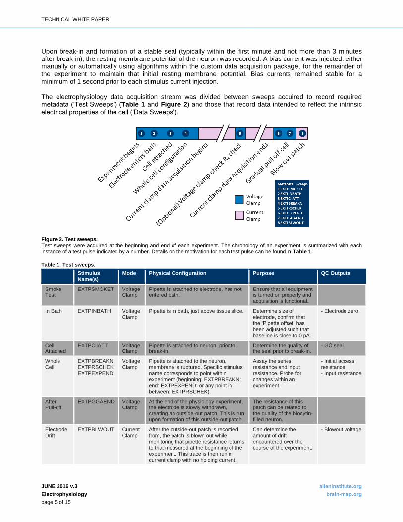
Upon break-in and formation of a stable seal (typically within the first minute and not more than 3 minutes after break-in), the resting membrane potential of the neuron was recorded. A bias current was injected, either manually or automatically using algorithms within the custom data acquisition package, for the remainder of the experiment to maintain that initial resting membrane potential. Bias currents remained stable for a minimum of 1 second prior to each stimulus current injection. The electrophysiology data acquisition stream was divided between sweeps acquired to record required metadata (‘Test Sweeps’) (Table 1 and Figure 2) and those that record data intended to reflect the intrinsic electrical properties of the cell (‘Data Sweeps’).

Figure 2. Test sweeps. Test sweeps were acquired at the beginning and end of each experiment. The chronology of an experiment is summarized with each instance of a test pulse indicated by a number. Details on the motivation for each test pulse can be found in Table 1.

Table 1. Test sweeps.

Stimulus Name(s)

Mode Physical Configuration Purpose QC Outputs

Smoke Test

EXTPSMOKET Voltage Clamp

Pipette is attached to electrode, has not entered bath.

Ensure that all equipment is turned on properly and acquisition is functional.

In Bath EXTPINBATH Voltage Clamp

Pipette is in bath, just above tissue slice. Determine size of electrode, confirm that the ‘Pipette offset’ has been adjusted such that baseline is close to 0 pA.

- Electrode zero

Cell Attached

EXTPCllATT Voltage Clamp

Pipette is attached to neuron, prior to break-in.

Determine the quality of the seal prior to break-in.

- GΩ seal

Whole Cell

EXTPBREAKN EXTPRSCHEK EXTPEXPEND

Voltage Clamp

Pipette is attached to the neuron, membrane is ruptured. Specific stimulus name corresponds to point within experiment (beginning: EXTPBREAKN; end: EXTPEXPEND; or any point in between: EXTPRSCHEK).

Assay the series resistance and input resistance. Probe for changes within an experiment.

- Initial access resistance - Input resistance

After Pull-off

EXTPGGAEND Voltage Clamp

At the end of the physiology experiment, the electrode is slowly withdrawn, creating an outside-out patch. This is run upon formation of this outside-out patch.

The resistance of this patch can be related to the quality of the biocytin-filled neuron.

Electrode Drift

EXTPBLWOUT Current Clamp

After the outside-out patch is recorded from, the patch is blown out while monitoring that pipette resistance returns to that measured at the beginning of the experiment. This trace is then run in current clamp with no holding current.

Can determine the amount of drift encountered over the course of the experiment.

- Blowout voltage




page 6 of 15

ELECTROPHYSIOLOGY STIMULI STRATEGY AND DETAILS Different sets of stimulation waveforms were used in order to (Table 2 and Figure 3): A. Interrogate intrinsic membrane mechanisms that underlie the input/output function of neurons A1. Linear and non-linear subthreshold properties A2. Action potential initiation and propagation

A3. Afterhyperpolarization/afterdepolarization

B. Understand aspects of neural response properties in vivo B1. Stimulation frequency dependence (theta vs. gamma) of spike initiation mechanisms B2. Ion channel states due to different resting potentials in vivo C. Construct and test computational models of varying complexity emulating the neural response to stereotyped stimuli C1. Generalized leaky-integrate-and-fire (GLIF) models

C2. Biophysically and morphologically realistic conductance-based compartmental models

Table 2. Goal per stimulus-set lookup table.

A1 A2 A3 B1 B2 C1 C2

Ramp X X X X

Long Square X X X

Short Square X X X

Short Square - Hold X X

Short Square - Triple X

Noise (1 & 2) X X

Ramp to Rheobase X X

Square Suprathreshold X X

Square Subthreshold X X

Note: Columns titled across the top row correspond to the goals described above.




page 7 of 15

Figure 3. Electrophysiology stimulus descriptions and details. The square 2 s suprathreshold and 0.5 ms subthreshold stimuli are further described in the Biophysical Model-perisomatic whitepaper located in “Documentation.”

Ramp

Long Square

Short Square

Noise 1 & 2

Square 0.5 ms Subthreshold

Description: Current injection of increasing intensity at a rate much slower than the time constant of the neuron. Details: Ramp of 25 pA per 1 second, terminated after a series of action potentials are acquired.

Short Square Hold -60mV Hold -70mV Hold -80mV

Short Square Triple

Noise Ramp to Rheobase

Square 2 s Suprathreshold

Description: Square pulse of a duration to allow the neuron to come to steady-state. Details: 1 s current injections from -110 pA (or -190 for some Pvalb neurons) to rheobase + 160 pA, in 20 pA increments.

Description: Square pulse brief enough to elicit a single action potential. Details: 3 ms current injections used to find the action potential threshold within 10 pA.

Description: Short pulse stimulus with stepped holding potentials. Details: Bias current brings the neuron to steady state potentials of -60 mV or -80 mV. If the neuron rests at -80 mV or -60 mV, the neuron is held at -70 mV.

Description: Three short pulse stimuli in rapid succession. Details: Three threshold stimuli of 3 ms duration are delivered at decreasing frequencies from ~140 Hz to ~30 Hz.

Description: Noise pulses offset with square current injections. Details: Pink noise generated from 2 seeds (1 & 2) scaled to three

amplitudes, 0.75, 1, and 1.5 times rheobase. Additional details can be found in the Appendix.

Description: Noise pulse offset with a ramp to rheobase current injection. Details: Noise with varying coefficients of variation, scaled to rheobase. Additional details can be found in the Appendix.

Description: Suprathreshold long square current injections to analyze

sustained action potential firing. Details: 2 s square current injections to rheobase + 40 pA and 80 pA. Additional details can be found in the Biophysical Models - perisomatic Technical White Paper.

Description: Brief subthreshold square current injections used to determine membrane capacitance for biophysical models. Details: 0.5 ms square current injections to +/- 200 pA. Additional

details can be found in the Biophysical Models - perisomatic Technical White Paper.

http://help.corp.alleninstitute.org/display/celltypes/Documentation




page 8 of 15

ELECTROPHYSIOLOGY DATA CURATION AND QUALITY EVALUATION Before data was subjected to additional analysis, the electrophysiology data underwent two sets of QC standards, at the cell and the sweep levels. Electrophysiology Data Qualification Gate: Cell Level For a recording to be included for analysis, the following criteria must be met:

Electrode must be ‘zeroed’ before recording. Measurement: Baseline of EXTPINBATH sweep must be 0 +/- 100 pA.

A GΩ seal must have been reached prior to break-in. Measurement: Steady state resistance in EXTPCllATT must be > 1.0 GΩ.

The initial access resistance must be < 20 MΩ or 15% of the Rinput. Measurement: Rinput and Raccess measured in EXTPBREAKN data pulse.

Electrode drift: The final voltage recording must be within 1 mV for every 10 minutes of data recording. Measurement: Final voltage measured with EXTPBLWOUT.

Electrophysiology Data Qualification Gate: Sweep Level For a single sweep within a recording to be included for analysis, the following criteria must be met:

Bridge balance setting must be < 20 MΩ or 15% of the Rinput. Bias current injection must be 0 +/- 100 pA. High frequency noise/patch instability RMS noise measurements in a short window (1.5 ms, to gauge

high frequency noise) and longer window (500 ms, to measure patch instability) must be less than 0.07 mV and 0.5 mV, respectively.

Voltage stability: The voltage immediately prior to the stimulus (measured over a 500 ms window) and the voltage measured at the end of the data pulse (measured over 500 ms) must be within 1 mV of each other. In a small number of sweeps from early experiments where the recovery period following a stimulus was not long enough for this to be an appropriate metric, a modified automated voltage stability measure was used–either shortening the final averaging window to 200 ms or fitting a linear regression to the final 1 second of data and determining if the membrane potential would return to baseline within 5 seconds.

Manual Electrophysiology Data Review At the beginning of every data sweep, a short test pulse was delivered to gauge whether the correct bridge balance setting was applied. Following every experiment, test pulses were checked by an independent observer and any sweeps that were deemed to have unsatisfactory bridge balance compensation (existence of a clear DC offset, relative to the test pulse from the first data trace, indicative of an increased access resistance) were failed from the data set. Electrophysiology Data Quality Assessment – Cell Health

The current QC criteria (described above) are based on typical metrics of stable electrophysiology recordings. Currently, other features of electrophysiology recordings, that may be indicative of cell health, are not being utilized to exclude data. These include excitability that may be considered abnormal, such as the inability to sustain firing at modest levels of current injection, as well as subthreshold and suprathreshold properties that may change during the course of a recording, due to dialysis of critical intracellular components, plasticity due to the preceding stimulus sets, or a combination of these factors. Neurons exhibiting these behaviors are being analyzed for cross-modal indicators of cell health, and internal investigations are underway to better understand the observed changes in excitability. In the future, data quality standards and curation metrics will evolve, and may include classification based on these results.




page 9 of 15

WHOLE-CELL ELECTROPHYSIOLOGY FEATURE ANALYSIS Electrophysiological data collected from individual whole-cell recordings consisted of high temporal resolution time series of membrane potential (in current-clamp mode) and trans-membrane current measurements (in voltage-clamp mode). For the Allen Cell Types Database, the data were primarily collected in current-clamp mode to determine the basic subthreshold and suprathreshold electrical behavior of various cell types. As different types of cells fire action potentials of various shapes and with a range of firing patterns (McCormick et al., 1986; Ascoli et al., 2008), in addition to responding in different ways to subthreshold stimulation, it is useful to characterize the basic features of these responses in a consistent way. Here we describe the specific analyses of electrophysiological data that were used to calculate the specific features of suprathreshold and subthreshold responses of the recorded cells. Action Potential Identification The first step in feature analysis was to identify if and when action potentials occurred during a recorded electrophysiological sweep. Only sweeps that passed sweep-level quality control were analyzed. The time derivative of the voltage trace (dV/dt) was used to initially detect action potentials. To produce this derivative, the voltage trace was smoothed with a digital four-pole Bessel filter with a cutoff frequency of 10 kHz, and the point-by-point difference was calculated and divided by the time interval between points. Putative action potential events were identified where the derivative trace exceed 20 mV/ms and where the time derivative returned below 0 mV/ms between consecutive events. For each of these events, the maximum voltage before the next event was identified as the peak of the putative action potential. Next, the maximum dV/dt was identified in the interval between the time of the initial detected event and the time of the peak voltage. Then, the time of the action potential threshold was first estimated by finding the point before the peak where the dV/dt was 5% of the maximum dV/dt (note this initial estimate was refined after the action potential detection phase-see below). With these initial estimates of action potential threshold and peak, several criteria were applied to rule out events that were not action potentials. If the time between the threshold and the peak exceeded 2 ms, the putative action potential was rejected. Similarly, if the difference between the threshold voltage and the peak was less than 2 mV, or if the absolute peak was less than –30 mV, the putative action potential was also rejected. This was to avoid treating brief, occasional voltage transients as action potentials, while still reliably detecting small action potentials that could be evoked by continuous, strong stimulation of certain types of cells. Single Action Potential Features Once the list of action potentials was refined, specific features of each action potential were calculated (Figure 4). First, the estimate of the threshold voltage was refined by finding the point where the dV/dt matched 5% of the average maximal dV/dt across all action potentials in a given sweep. This average was used instead of the per-action potential maximum dV/dt because some short action potentials evoked by long, strong stimuli had significantly lower maximum dV/dt values that led to the identified threshold voltage being too hyperpolarized. This method based on a fraction of maximum dV/dt can produce more consistent estimates of threshold across the cells of the same type compared to one based on an absolute dV/dt level (Jackson et al., 2004), and it can also be reliably applied across responses to a variety of stimuli. The time of threshold, threshold voltage, and level of injected current at threshold were recorded for each action potential. The time of the action potential was defined as the time of the action potential threshold. Several other features were also calculated for every action potential. Minimum and maximum values were calculated from the original voltage trace, except those calculated from dV/dt trace, which was generated by smoothing and differentiation as described above. The term “trough” has been used here to describe features of the action potential after the action potential rather than the term “after-hyperpolarization” since in many cases the membrane potential did not hyperpolarize below the baseline membrane potential. For most of the following values, both a voltage value and time value were extracted.




page 10 of 15

Action potential peak: Maximum value of the membrane potential during the action potential (i.e. between the action potential’s threshold and the time of the next action potential, or end of the response). Action potential trough: Minimum value of the membrane potential in the interval between the peak and the time of the next action potential. Action potential fast trough: Minimum value of the membrane potential in the interval lasting 5 ms after the peak. Action potential slow trough: Minimum value of the membrane potential in the interval from 5 ms after the peak until the time of the next action potential. If the time between the peak and the next action potential was less than 5 ms, this value was identical to the fast trough. Time of the slow trough: Ratio of the time interval between the action potential peak and the slow trough and the time interval between the action potential peak and the next action potential. Action potential height: The action potential height was defined as the difference between the action potential peak and the action potential trough. Action potential full width: The action potential full width was defined as the width at half-height. The points in the voltage trace on either side of the peak that matched half the action potential height were identified, and the width was defined as the time interval between these points. Action potential peak upstroke: The maximum value of dV/dt between the action potential threshold and the action potential peak. Action potential peak downstroke: The minimum value of dV/dt between the action potential peak and the action potential trough. Upstroke/downstroke ratio: The ratio between the absolute values of the action potential peak upstroke and the action potential peak downstroke.

Figure 4. Illustration of single action potential features. Action potential evoked by a long square stimulus with various features identified. See text for feature definitions.




page 11 of 15

Action Potential Train Features In addition to single action potential features, several features were calculated based on trains of action potentials (see Figure 5), which were often evoked by long current step stimuli. As action potential times are accessible in the Neurodata Without Borders (NWB) files (a standard file format for neurophysiology) available for download, spike train features other than those listed here can also be calculated by end users. Interspike interval (ISI): Difference in time between the time of an action potential and the time of the next consecutive action potential. First ISI: The ISI between the first two spikes evoked by a stimulus. Average ISI: The mean value of all interspike intervals in a sweep. ISI coefficient of variation: The coefficient of variation (CV, or standard deviation divided by the mean) of all interspike intervals in a sweep. Average firing rate: The number of spikes during a stimulus period divided by the duration of the stimulus period. Latency: Time between the start of the stimulus until the time of the first spike evoked by a stimulus. Adaptation index: The rate at which firing speeds up or slows down during a stimulus, defined as:

1

𝑁 − 1∑

𝐼𝑆𝐼𝑛+1 − 𝐼𝑆𝐼𝑛𝐼𝑆𝐼𝑛+1 + 𝐼𝑆𝐼𝑛

𝑁−1

𝑛=1

where N is the number of ISIs in the sweep. Delay: A spike train was defined as having a delayed start to firing if the latency was greater than the average ISI (reported as a true/false value). Burst: A spike train was defined as having a burst if its first two ISIs were both less than or equal to 5 ms (reported as a true/false value). Pause: A spike train was defined as having a pause if any ISI was more than 3 times the duration of the ISIs immediately before and after it (i.e., at least two spikes on average were “skipped”) (reported as a true/false value).

http://help.corp.alleninstitute.org/display/celltypes/API




page 12 of 15

Figure 5. Illustration of action potential train features. A. Sweep illustration of features such as latency, first ISI, and other ISIs. More complex features are calculated based on combinations of these features. B. Examples of sweeps containing a delay (top) and pauses (bottom).

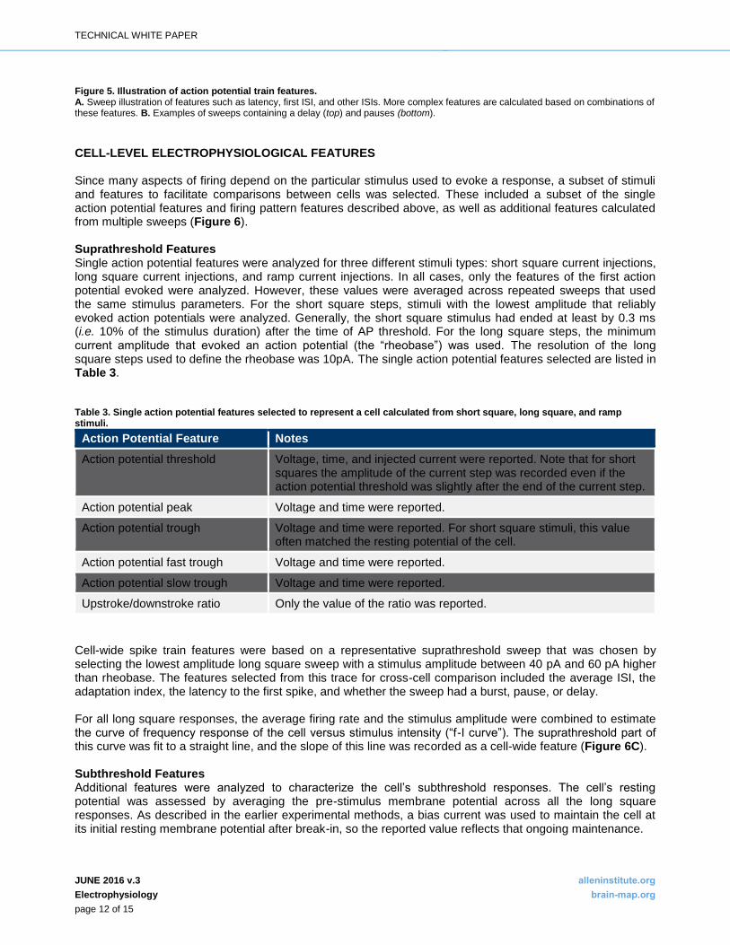
CELL-LEVEL ELECTROPHYSIOLOGICAL FEATURES Since many aspects of firing depend on the particular stimulus used to evoke a response, a subset of stimuli and features to facilitate comparisons between cells was selected. These included a subset of the single action potential features and firing pattern features described above, as well as additional features calculated from multiple sweeps (Figure 6). Suprathreshold Features Single action potential features were analyzed for three different stimuli types: short square current injections, long square current injections, and ramp current injections. In all cases, only the features of the first action potential evoked were analyzed. However, these values were averaged across repeated sweeps that used the same stimulus parameters. For the short square steps, stimuli with the lowest amplitude that reliably evoked action potentials were analyzed. Generally, the short square stimulus had ended at least by 0.3 ms (i.e. 10% of the stimulus duration) after the time of AP threshold. For the long square steps, the minimum current amplitude that evoked an action potential (the “rheobase”) was used. The resolution of the long square steps used to define the rheobase was 10pA. The single action potential features selected are listed in Table 3. Table 3. Single action potential features selected to represent a cell calculated from short square, long square, and ramp stimuli.

Action Potential Feature Notes

Action potential threshold Voltage, time, and injected current were reported. Note that for short squares the amplitude of the current step was recorded even if the action potential threshold was slightly after the end of the current step.

Action potential peak Voltage and time were reported.

Action potential trough Voltage and time were reported. For short square stimuli, this value often matched the resting potential of the cell.

Action potential fast trough Voltage and time were reported.

Action potential slow trough Voltage and time were reported.

Upstroke/downstroke ratio Only the value of the ratio was reported.

Cell-wide spike train features were based on a representative suprathreshold sweep that was chosen by selecting the lowest amplitude long square sweep with a stimulus amplitude between 40 pA and 60 pA higher than rheobase. The features selected from this trace for cross-cell comparison included the average ISI, the adaptation index, the latency to the first spike, and whether the sweep had a burst, pause, or delay. For all long square responses, the average firing rate and the stimulus amplitude were combined to estimate the curve of frequency response of the cell versus stimulus intensity (“f-I curve”). The suprathreshold part of this curve was fit to a straight line, and the slope of this line was recorded as a cell-wide feature (Figure 6C). Subthreshold Features Additional features were analyzed to characterize the cell’s subthreshold responses. The cell’s resting potential was assessed by averaging the pre-stimulus membrane potential across all the long square responses. As described in the earlier experimental methods, a bias current was used to maintain the cell at its initial resting membrane potential after break-in, so the reported value reflects that ongoing maintenance.




page 13 of 15

Other features made use of long square sweeps with negative current amplitudes that did not exceed 100 pA in magnitude (Figure 6A). The minimum membrane potentials during these responses were measured, and a linear fit was performed on these values and their respective stimulus amplitudes. The slope of the resulting fit was used as the estimate of the input resistance of the cell. In addition, these responses were fit with a single exponential curve between 10% of the maximum voltage deflection (in the hyperpolarizing direction) and the minimum membrane potential during the response. The time constants of these fits were averaged across steps to estimate the membrane time constant of the cell. The response to a negative-going current step in which the minimum membrane potential was closest to -100 mV was selected for analysis of the membrane “sag” that can occur due to hyperpolarization-activated cationic currents (Figure 6B). The difference in the resting potential between the minimum value and the steady-state value was divided by the peak deflection during the stimulus to calculate a sag fraction that varied from 0 (no sag) to 1 (complete return back to the resting potential). In some cells, it was difficult to hyperpolarize the cells to -100 mV due to their low input resistances, so in all cases the membrane potential at which the sag was evaluated was also reported. This value, as well as the baseline membrane potential before the stimulus (which varies across cells) should be incorporated into any analyses of the reported sag values by end users of the data.

Figure 6. Illustration of cell-wide features calculated across multiple sweeps. A. Illustration of features calculated from a series of subthreshold steps. The minimum values of the voltage are identified (middle, red dots), plotted versus the injected current, and fit with a line (left, red line) to estimate the input resistance. The baseline potential is shown by the dotted gray line on the leftmost plot. Single exponential fits (blue lines, middle) are made to these steps, and the time constants are plotted versus the injected current (right) and averaged (right, blue line). The voltage scale in the middle is the same as the right, and stimulus steps were one second long. B. Example of calculation of the sag, which equaled the return to steady state divided by the peak deflection. C. Illustration of an “f-I curve” along with the linear fit to the suprathreshold component that yielded the f-I curve slope feature. Data in panels A and B are from the same cell; data in C are from a different cell.

API ACCESS TO FEATURES

The data and computed features can be accessed via an application programmatic interface (API).

REFERENCES

http://help.corp.alleninstitute.org/display/celltypes/API




page 14 of 15

Ascoli GA, Alonso-Nanclares L, Anderson SA, Barrionuevo G, Benavides-Piccione R, Burkhalter A, Buzsáki G, Cauli B, Defelipe J, Fairén A, Feldmeyer D, Fishell G, Fregnac Y, Freund TF, Gardner D, Gardner EP, Goldberg JH, Helmstaedter M, Hestrin S, Karube F, Kisvárday ZF, Lambolez B, Lewis DA, Marin O, Markram H, Muñoz A, Packer A, Petersen CC, Rockland KS, Rossier J, Rudy B, Somogyi P, Staiger JF, Tamas G, Thomson AM, Toledo-Rodriguez M, Wang Y, West DC, Yuste R (2008) Petilla terminology: nomenclature of features of GABAergic interneurons of the cerebral cortex. Nature Reviews Neuroscience 9:557-568. Dong HW (2008) Allen Reference Atlas: A Digital Color Brain Atlas of the C57BL/6J Male Mouse. Hoboken, NJ: John Wiley & Sons. Jackson AC, Yao GL, Bean BP (2004) Mechanism of spontaneous firing in dorsomedial suprachiasmatic nucleus neurons. Journal of Neuroscience 24:7985-7998. McCormick DA, Connors BW, Lighthall JW, Prince DA (1985) Comparative electrophysiology of pyramidal and sparsely spiny stellate neurons of the neocortex. Journal of Neurophysiology 54:782–806. Neher E (1992) Correction for liquid junction potentials in patch clamp experiments. Methods Enzymology 207:123-131. Zhao S, Ting JT, Atallah HE, Qiu L, Tan J, Gloss B, Augustine GJ, Deisseroth K, Luo M, Graybiel AM, Feng G (2011) Cell type–specific channelrhodopsin-2 transgenic mice for optogenetic dissection of neural circuitry function. Nature Methods 8:745-752.




page 15 of 15

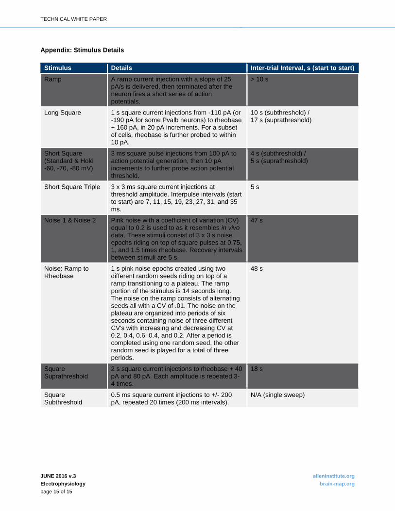
Appendix: Stimulus Details

Stimulus Details Inter-trial Interval, s (start to start)

Ramp A ramp current injection with a slope of 25 pA/s is delivered, then terminated after the neuron fires a short series of action potentials.

> 10 s

Long Square 1 s square current injections from -110 pA (or -190 pA for some Pvalb neurons) to rheobase + 160 pA, in 20 pA increments. For a subset of cells, rheobase is further probed to within 10 pA.

10 s (subthreshold) / 17 s (suprathreshold)

Short Square (Standard & Hold -60, -70, -80 mV)

3 ms square pulse injections from 100 pA to action potential generation, then 10 pA increments to further probe action potential threshold.

4 s (subthreshold) / 5 s (suprathreshold)

Short Square Triple 3 x 3 ms square current injections at threshold amplitude. Interpulse intervals (start to start) are 7, 11, 15, 19, 23, 27, 31, and 35 ms.

5 s

Noise 1 & Noise 2 Pink noise with a coefficient of variation (CV) equal to 0.2 is used to as it resembles in vivo data. These stimuli consist of 3 x 3 s noise epochs riding on top of square pulses at 0.75, 1, and 1.5 times rheobase. Recovery intervals between stimuli are 5 s.

47 s

Noise: Ramp to Rheobase

1 s pink noise epochs created using two different random seeds riding on top of a ramp transitioning to a plateau. The ramp portion of the stimulus is 14 seconds long. The noise on the ramp consists of alternating seeds all with a CV of .01. The noise on the plateau are organized into periods of six seconds containing noise of three different CV's with increasing and decreasing CV at 0.2, 0.4, 0.6, 0.4, and 0.2. After a period is completed using one random seed, the other random seed is played for a total of three periods.

48 s

Square Suprathreshold

2 s square current injections to rheobase + 40 pA and 80 pA. Each amplitude is repeated 3-4 times.

18 s

Square Subthreshold

0.5 ms square current injections to +/- 200 pA, repeated 20 times (200 ms intervals).

N/A (single sweep)

allen cell types database - help

Documents