alphaview software user guide - university of south florida · alphaview software user guide...
TRANSCRIPT

page 1
Formerly Cell Biosciences
AlphaView Software User Guide
Copyright © 2011 ProteinSimple. All rights reserved.
ProteinSimple3040 Oakmead Village DriveSanta Clara, CA 95051Toll-free: (888) 607-9692Tel: (408) 510-5500Fax: (408) 510-5599email: [email protected]: www.proteinsimple.com
AlphaView Software User Guide

AlphaView Software User Guide
P/N 94-13934-00
Revision 3a, July 2011
For research use only. Not for use in diagnostic procedures
Patents and Trademarks Automatic Image Capture (AIC) and digital ProteomeChip technology are covered by U.S. Patent Nos 6,995,901, 6,909,459, 6,853,454, 6,271,042, 7,166,202, and other issued and pending patents in the U.S. and other countries. ProteinSimple, the ProteinSimple logo, the Alpha Innotech logo, Protein Forest, the Protein Forest logo, the AIC logo, AlphaCal, AlphaImager, AlphaPart11View, AlphaQuant, AlphaSnap, AlphaSpec, AlphaUV, AlphaView, ChemiGlow, Chromalight, dPC, digital ProteomeChip, FluorChem, MSRAT, MultiImage, NanoPro, the intertwined helix design, iWB, ProteomeChip, red, SpectraPlex, Xpedition, XplorBright, and XplorUV are trademarks or registered trademarks of ProteinSimple. Other marks appearing in these materi-als are marks of their respective owners.
AlphaView Software User Guide

page i
Table of Contents
Chapter 1:Introduction . . . . . . . . . . . . . . . . . . . . . . . . . . . . . . 1
Introducing AlphaView. . . . . . . . . . . . . . . . . . . . . . . . . . . 2
Mouse Functions . . . . . . . . . . . . . . . . . . . . . . . . . . . 2
Starting AlphaView Software. . . . . . . . . . . . . . . . . . 2
System Information . . . . . . . . . . . . . . . . . . . . . . . . . 2
About This Manual . . . . . . . . . . . . . . . . . . . . . . . . . . . . . 3
Customer Service and Technical Support. . . . . . . . . . . . 4
Chapter 2:Getting Started—Basic Imaging Functions . . 5
Basic Imaging Functions . . . . . . . . . . . . . . . . . . . . . . . . . 6
Contrast Adjustments . . . . . . . . . . . . . . . . . . . . . . . . . . . 6
Using the Contrast Adjustments Tools for Grayscale Images . . . . . . . . . . . . . . . . . . . . . . . . . . . . . . . . . . . 7
Multicolor Image Display . . . . . . . . . . . . . . . . . . .13
Automatic Enhancement . . . . . . . . . . . . . . . . . . .16
Imaging Tools. . . . . . . . . . . . . . . . . . . . . . . . . . . . . . . . .17
Tool Bar . . . . . . . . . . . . . . . . . . . . . . . . . . . . . . . . .17
Compare View . . . . . . . . . . . . . . . . . . . . . . . . . . . .19
Tool Box . . . . . . . . . . . . . . . . . . . . . . . . . . . . . . . . .22
Status Bar . . . . . . . . . . . . . . . . . . . . . . . . . . . . . . .22
Chapter 3:Drop-Down Menus . . . . . . . . . . . . . . . . . . . . . . . 23
Main Menu . . . . . . . . . . . . . . . . . . . . . . . . . . . . . . . . . .24
File Menu. . . . . . . . . . . . . . . . . . . . . . . . . . . . . . . . . . . . 24
File > Open Menu . . . . . . . . . . . . . . . . . . . . . . . . 24
File > Save/Load Analysis . . . . . . . . . . . . . . . . . . . 26
File > Close Menu. . . . . . . . . . . . . . . . . . . . . . . . . 26
File Save, Save As, Save Modified, and Save All Menus . . . . . . . . . . . . . . . . . . . . . . . . . . . . . . . . . . 26
Print . . . . . . . . . . . . . . . . . . . . . . . . . . . . . . . . . . . . 28
Printer Setup . . . . . . . . . . . . . . . . . . . . . . . . . . . . . 28
Exit Function . . . . . . . . . . . . . . . . . . . . . . . . . . . . . 29
Edit Menu . . . . . . . . . . . . . . . . . . . . . . . . . . . . . . . . . . . 30
Edit Activation . . . . . . . . . . . . . . . . . . . . . . . . . . . . 30
Copy and Crop . . . . . . . . . . . . . . . . . . . . . . . . . . . 31
Reset and Clear Options . . . . . . . . . . . . . . . . . . . 31
Image Menu . . . . . . . . . . . . . . . . . . . . . . . . . . . . . . . . . 31
Overlay . . . . . . . . . . . . . . . . . . . . . . . . . . . . . . . . . . 32
Extract Channels. . . . . . . . . . . . . . . . . . . . . . . . . . 32
Channel Viewer . . . . . . . . . . . . . . . . . . . . . . . . . . . 32
Equalize . . . . . . . . . . . . . . . . . . . . . . . . . . . . . . . . . 33
Arithmetic . . . . . . . . . . . . . . . . . . . . . . . . . . . . . . . 33
Conversion . . . . . . . . . . . . . . . . . . . . . . . . . . . . . . . 34
Flat Field Calibrate - Manual . . . . . . . . . . . . . . . . 35
Register Channels . . . . . . . . . . . . . . . . . . . . . . . . . 35
Resize Image . . . . . . . . . . . . . . . . . . . . . . . . . . . . . 36
Image Information. . . . . . . . . . . . . . . . . . . . . . . . . 37
Setup Menu. . . . . . . . . . . . . . . . . . . . . . . . . . . . . . . . . . 37
AlphaView Software User Guide

page ii
Print Info . . . . . . . . . . . . . . . . . . . . . . . . . . . . . . . . .38
Print Mode . . . . . . . . . . . . . . . . . . . . . . . . . . . . . . .39
Print Date. . . . . . . . . . . . . . . . . . . . . . . . . . . . . . . .39
Preferences. . . . . . . . . . . . . . . . . . . . . . . . . . . . . . .39
Overlay Menu . . . . . . . . . . . . . . . . . . . . . . . . . . . . . . . .42
Load Overlay . . . . . . . . . . . . . . . . . . . . . . . . . . . . .42
Save Overlay . . . . . . . . . . . . . . . . . . . . . . . . . . . . .42
Show Annotation . . . . . . . . . . . . . . . . . . . . . . . . . .43
Utilities Menu . . . . . . . . . . . . . . . . . . . . . . . . . . . . . . . .43
Notepad. . . . . . . . . . . . . . . . . . . . . . . . . . . . . . . . .44
Explorer . . . . . . . . . . . . . . . . . . . . . . . . . . . . . . . . .44
View Menu. . . . . . . . . . . . . . . . . . . . . . . . . . . . . . . . . . .45
Default Tools Position . . . . . . . . . . . . . . . . . . . . . .46
Zoom Functions. . . . . . . . . . . . . . . . . . . . . . . . . . .47
Window Menu. . . . . . . . . . . . . . . . . . . . . . . . . . . . . . . .47
Help Menu . . . . . . . . . . . . . . . . . . . . . . . . . . . . . . . . . .48
Chapter 4:Image Enhancement Tools . . . . . . . . . . . . . . . 49
Tool Box Enhancement Tab. . . . . . . . . . . . . . . . . . . . .50
Zoom . . . . . . . . . . . . . . . . . . . . . . . . . . . . . . . . . . . . . . .50
Histogram . . . . . . . . . . . . . . . . . . . . . . . . . . . . . . . . . . .51
Rotate-Flip . . . . . . . . . . . . . . . . . . . . . . . . . . . . . . . . . . .53
Annotate . . . . . . . . . . . . . . . . . . . . . . . . . . . . . . . . . . . .54
Object Attributes . . . . . . . . . . . . . . . . . . . . . . . . . .55
Drawing Tools . . . . . . . . . . . . . . . . . . . . . . . . . . . .59
Editing Tools. . . . . . . . . . . . . . . . . . . . . . . . . . . . . .61
False Color . . . . . . . . . . . . . . . . . . . . . . . . . . . . . . . . . . .63
Gray Scale (Palette 0) . . . . . . . . . . . . . . . . . . . . . .64
High–Low (Palette 1) . . . . . . . . . . . . . . . . . . . . . .64
Other Palettes . . . . . . . . . . . . . . . . . . . . . . . . . . . .64
Filter . . . . . . . . . . . . . . . . . . . . . . . . . . . . . . . . . . . . . . . . 66
General Information . . . . . . . . . . . . . . . . . . . . . . . 67
Sharpening Filters . . . . . . . . . . . . . . . . . . . . . . . . . 68
Noise Filters . . . . . . . . . . . . . . . . . . . . . . . . . . . . . . 68
Despeckle Filters . . . . . . . . . . . . . . . . . . . . . . . . . . 68
3-D (Contour) Filters . . . . . . . . . . . . . . . . . . . . . . . 69
Smoothing Filters . . . . . . . . . . . . . . . . . . . . . . . . . . 70
Edge Filters . . . . . . . . . . . . . . . . . . . . . . . . . . . . . . 70
Horizontal Edge Filter . . . . . . . . . . . . . . . . . . . . . . 70
Vertical Edge Filter . . . . . . . . . . . . . . . . . . . . . . . . 70
Custom Filter . . . . . . . . . . . . . . . . . . . . . . . . . . . . . 71
Undo Button . . . . . . . . . . . . . . . . . . . . . . . . . . . . . 71
Examples of Filter Results . . . . . . . . . . . . . . . . . . 71
Movie Mode . . . . . . . . . . . . . . . . . . . . . . . . . . . . . . . . . 71
Chapter 5:Image Analysis Tools . . . . . . . . . . . . . . . . . . . . . 73
Tool Box Analysis Tools Tab. . . . . . . . . . . . . . . . . . . . . 74
Molecular Weight Determination . . . . . . . . . . . . . . . . 74
Entering Known Molecular Weights for Markers . . . . . . . . . . . . . . . . . . . . . . . . . . . . . . . . . 76
Determining Molecular Weights of Unknown Bands . . . . . . . . . . . . . . . . . . . . . . . . . . . . . . . . . . . 77
Using the Molecular Weight Standards Library. . 79
Special Functions . . . . . . . . . . . . . . . . . . . . . . . . . . 81
The Graph Tool . . . . . . . . . . . . . . . . . . . . . . . . . . . 82
Colony Count. . . . . . . . . . . . . . . . . . . . . . . . . . . . . . . . . 83
Editing Tools . . . . . . . . . . . . . . . . . . . . . . . . . . . . . 87
Spot Count Data . . . . . . . . . . . . . . . . . . . . . . . . . . 89
Multiplex Band Analysis . . . . . . . . . . . . . . . . . . . . . . . . 90
Creating an Object Area of Interest. . . . . . . . . . . 90
AlphaView Software User Guide
page iii
Magic Wand and AutoSpot (Single Channel Only) . . . . . . . . . . . . . . . . . . . . . .92
Manipulating Objects . . . . . . . . . . . . . . . . . . . . . .96
Multiplex Band Analysis Measurements . . . . . . .97
Mass Standard Calibration Curves for Quantitative PCR . . . . . . . . . . . . . . . . . . . . . . . . 108
Lane Profile . . . . . . . . . . . . . . . . . . . . . . . . . . . . . . . . 114
Profile Path Width . . . . . . . . . . . . . . . . . . . . . . . 114
Auto Lane Detection Using an Area of Interest115
Manual Lane Detection . . . . . . . . . . . . . . . . . . 115
Bands Darker than Background Option. . . . . . 117
Image Analysis–Detect Bands . . . . . . . . . . . . . 117
Viewing Results . . . . . . . . . . . . . . . . . . . . . . . . . 117
Gel Smiling Correction . . . . . . . . . . . . . . . . . . . . 131
Molecular Weight Tab . . . . . . . . . . . . . . . . . . . 135
Mass Standards . . . . . . . . . . . . . . . . . . . . . . . . . 139
Advanced Lane Profile Options. . . . . . . . . . . . . 144
Common Features . . . . . . . . . . . . . . . . . . . . . . . 154
Additional Analysis Tools. . . . . . . . . . . . . . . . . . . . . . 158
The Ruler Function. . . . . . . . . . . . . . . . . . . . . . . 159
The Scoring Function . . . . . . . . . . . . . . . . . . . . . 160
Manual Count . . . . . . . . . . . . . . . . . . . . . . . . . . 162
Analyzing Arrays . . . . . . . . . . . . . . . . . . . . . . . . 164
Lane Profile - Advanced . . . . . . . . . . . . . . . . . . 168
Common Export Result Feature . . . . . . . . . . . . 168
Appendix A:AlphaView Molecular Weight Library Files.171
List of Standards . . . . . . . . . . . . . . . . . . . . . . . . . . . . 172
Appendix B:Data Description Tables . . . . . . . . . . . . . . . . . .175
Single Channel Columns . . . . . . . . . . . . . . . . . . . . . . .176
Multichannel Columns . . . . . . . . . . . . . . . . . . . . . . . .177
Appendix C:Data Interpretation . . . . . . . . . . . . . . . . . . . . . . .181
Loading Controls . . . . . . . . . . . . . . . . . . . . . . . . . . . . .182
Appendix D:Fully Worked Examples of Multicolor Band Analysis . . . . . . . . . . . . . . . . . . . . . . . . . . . . . . . . . .185
Example 1: Phosphorylation . . . . . . . . . . . . . . . . . . .186
Example 2: Quantitation Across Color Channels . . .192
AlphaView Software User Guide

page iv
AlphaView Software User Guide

page 1
Chapter 1:
Introduction
Chapter Overview• Introducing AlphaView
• About This Manual
• Customer Service and Technical Support
AlphaView Software User Guide

page 2 Chapter 1: Introduction
Introducing AlphaViewAlphaView® provides the utmost ease of use while offering comprehensive and versatile tools for capturing, analyzing, and annotating images. With a simple to use graphical user interface coupled with new and improved features, ProteinSimple has pioneered the most intuitive image capture and analysis software available.
AlphaView’s new and improved features include multiple image viewing, the ability to save analyses, and an enhanced movie mode. With our suite of analysis tools, you can perform molecular weight calculations, Rf determination, lane profile densitometry, multiplex band analysis, microtiter plate reading, object distance measuring, gel scoring, and automatic colony counting.
In addition, AlphaView’s image optimization tools can adjust contrast automatically or manually, convert images from positive to negative using digital filters, apply false color, and utilize many other techniques to clarify difficult-to-see portions of the image. Notes, labels, arrows, lines, and other drawing tools can be recorded directly onto the image using AlphaView’s annotation features. Annotations are superimposed on the image upon hard copy printing and can either be saved as a template file or as part of the image itself. All AlphaView features are accessible via convenient on-screen buttons and menus in an intuitive interface.
Images can be printed using a 256-level gray scale thermal printer or any printer with a Windows® driver. The low-cost, high-quality prints are ideal for lab notebook records or publication.
Mouse Functions
The system comes packaged with a two-button mouse. The left button activates functions and makes selec-tions when using the software. In some cases, the right mouse button can recall or reactivate the function that was most recently assigned to the left mouse button.
Starting AlphaView Software
To start AlphaView software, double-click the AlphaView software icon on the Windows desktop.
System Information
To display system information, click Help > About. This option accesses a pop-up box (see Figure 1-1).
AlphaView Software User Guide

About This Manual page 3
Figure 1-1: System Information
This box shows the software version number. Use the information specific to your instrument and software when calling ProteinSimple for technical support and software upgrades.
To close the box, click on the OK button.
About This ManualThis manual uses different fonts to indicate certain conditions:
• Bold text indicates the name of a button, a menu, or a function found in a menu.
• Courier text indicates an entry that is typed.
• Letters or words found between < > refer to keys on the keyboard.
• NOTE indicates key points and useful hints.
• CAUTION and !WARNING! statements indicate actions that may either harm the system or user, or affect the data quality.
• Icons or buttons to be pushed are placed next to their respective descriptions in the text.
AlphaView Software User Guide

page 4 Chapter 1: Introduction
Customer Service and Technical Support Telephone(408) 510-5500 (888) 607-9692 (toll free)
Fax(408) 510-5599
Webwww.proteinsimple.com
AddressProteinSimple 3040 Oakmead Village Drive Santa Clara, CA 95051USA
AlphaView Software User Guide

page 5
Chapter 2:
Getting Started—Basic Imaging Functions
Chapter Overview• Basic Imaging Functions
• Contrast Adjustments
• Imaging Tools
AlphaView Software User Guide

page 6 Chapter 2: Getting Started—Basic Imaging Functions
Basic Imaging FunctionsWhen the system computer is powered up, you can click on the AlphaView icon on the desktop to automat-ically open the AlphaView software. The following screen (Figure 2-1) displays:
Figure 2-1: AlphaView Screen—Displaying the Image Area and Display Controls
AlphaView software has four main control areas:
• Contrast Adjustments for image adjustment
• Enhancement Tools for image enhancement
• Analysis Tools for image analysis
Contrast AdjustmentsThe Contrast Adjustments window allows for the best visualization possible of a sample utilizing the black, white, and gamma adjustments, as well as, image reverse and auto contrast.
AlphaView Software User Guide
Contrast Adjustments page 7
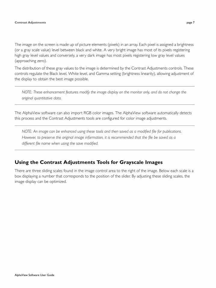
The image on the screen is made up of picture elements (pixels) in an array. Each pixel is assigned a brightness (or a gray scale value) level between black and white. A very bright image has most of its pixels registering high gray level values and conversely, a very dark image has most pixels registering low gray level values (approaching zero).
The distribution of these gray values to the image is determined by the Contrast Adjustments controls. These controls regulate the Black level, White level, and Gamma setting (brightness linearity), allowing adjustment of the display to obtain the best image possible.
NOTE: These enhancement features modify the image display on the monitor only, and do not change the original quantitative data.
The AlphaView software can also import RGB color images. The AlphaView software automatically detects this process and the Contrast Adjustments tools are configured for color image adjustments.
NOTE: An image can be enhanced using these tools and then saved as a modified file for publications. However, to preserve the original image information, it is recommended that the file be saved as a different file name when using the save modified.
Using the Contrast Adjustments Tools for Grayscale Images
There are three sliding scales found in the image control area to the right of the image. Below each scale is a box displaying a number that corresponds to the position of the slider. By adjusting these sliding scales, the image display can be optimized.
AlphaView Software User Guide
page 8 Chapter 2: Getting Started—Basic Imaging Functions
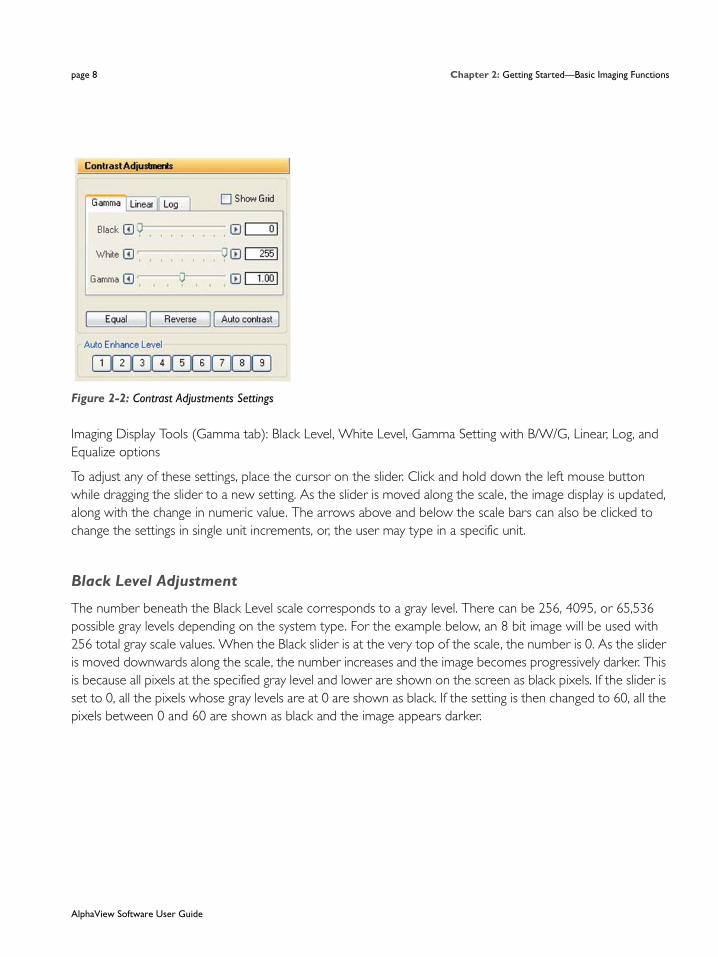
Figure 2-2: Contrast Adjustments Settings
Imaging Display Tools (Gamma tab): Black Level, White Level, Gamma Setting with B/W/G, Linear, Log, and Equalize options
To adjust any of these settings, place the cursor on the slider. Click and hold down the left mouse button while dragging the slider to a new setting. As the slider is moved along the scale, the image display is updated, along with the change in numeric value. The arrows above and below the scale bars can also be clicked to change the settings in single unit increments, or, the user may type in a specific unit.
Black Level Adjustment
The number beneath the Black Level scale corresponds to a gray level. There can be 256, 4095, or 65,536 possible gray levels depending on the system type. For the example below, an 8 bit image will be used with 256 total gray scale values. When the Black slider is at the very top of the scale, the number is 0. As the slider is moved downwards along the scale, the number increases and the image becomes progressively darker. This is because all pixels at the specified gray level and lower are shown on the screen as black pixels. If the slider is set to 0, all the pixels whose gray levels are at 0 are shown as black. If the setting is then changed to 60, all the pixels between 0 and 60 are shown as black and the image appears darker.
AlphaView Software User Guide

Contrast Adjustments page 9
Figure 2-3: Black Level Adjustment Example
White Level Adjustment
The number beneath the White Level scale also corresponds to a gray scale value. When the slider is at the very bottom of the scale, this number is 255. As the slider is moved upwards along the scale, the number decreases and the image becomes progressively lighter. This is because all pixels at the specified gray level value and above are shown on the screen as white pixels. For example, if the slider is set to 150, all the pixels between 150 and 255 are shown as white and the image appears lighter.
Figure 2-4: White Level Adjustment Example
Gamma Setting Adjustment
Changing the Gamma setting affects the image brightness by adjusting the linearity of the image on the screen and printouts, but does not affect quantitative data.
The camera sees objects linearly while the human eye does not. When the Gamma setting is set to a value of 1, the image is displayed as the camera sees it. This, however, is different from what the human eye detects. By adjusting the Gamma setting, the user can make the image on the screen correspond to what is seen when he/she looks directly at the object. We recommend a Gamma setting of 0.55 for best visual representation.
AlphaView Software User Guide

page 10 Chapter 2: Getting Started—Basic Imaging Functions
Figure 2-5: Gamma Setting Adjustment Example
The Auto Contrast Selection
The Auto Contrast feature will automatically scale the black and white values of an image to more tightly fit the gray scale intensity profiles (histogram). This selection will use different black and white values for different images depending upon their unique histograms. A more dramatic visual change will take place for low light level images (such as chemiluminescence) where smaller portions of the histogram are used. This selection can be turned on or off and will adjust differently for each image.
The Reverse Button
The Reverse button inverts the gray levels of the displayed image, converting a positive image to negative, or vice versa. For instance, an image with black bands on a white background is converted into an image with white bands on a black background by simply clicking the Reverse button. Clicking the button a second time returns the image to its original form.
Figure 2-6: Original Image vs. Reversed Image
AlphaView Software User Guide

Contrast Adjustments page 11
NOTE: Reversing an image changes the way it is displayed on the screen, but does not change the quantitative data. For example, the bands in the above gel have the same density, regardless of whether the gel is displayed as white bands on a black background or black bands on a light background. For information on reversing pixel values, see Chapter 5, “Image Analysis Tools“.
The Equal Button
The Equal button flattens the image to show all pixel values in the original image. Equal automatically adjusts the image display for maximum contrast which is beneficial for faint band detection.
Figure 2-7: Original and Equal Image
Making Linear, Log, or Equal Adjustments
Figure 2-8 shows an original image of film using default BWG settings.
Figure 2-8: Original Image of Film with Default BWG Settings
AlphaView Software User Guide

page 12 Chapter 2: Getting Started—Basic Imaging Functions
Figure 2-9 shows the image of film with linear Contrast Adjustments selected. The Linear tab provides mini-mum and maximum adjustment tools from 0 to 100%. Linear stretches the grayscale range of the displayed image to the system dynamic range of 0-65,535 grayscales.
Figure 2-9: Contrast Adjustments—Linear Tab Settings
Figure 2-10 shows the image of film with log the Contrast Adjustments selected the log provides minimum and maximum adjustment tools from 0 to 100%. The Log performs a logarithmic adjustment to the grayscale range of the displayed image.
Figure 2-10: Contrast Adjustments—Log Tab
Figure 2-11 shows the image of film with equal Contrast Adjustments selected. The Equal option automati-cally adjusts the image display for maximum contrast which is beneficial for faint band detection.
AlphaView Software User Guide

Contrast Adjustments page 13
Figure 2-11: Contrast Adjustments—Image of Film with Equal Contrast Adjustment
Multicolor Image Display
Channel Viewer
The Channel Viewer performs a preliminary review of a composite display of a multichannel image to view each channel separately in the context of the composite image. While each channel may also be displayed as a single channel using the Contrast Adjustments window, the Channel Viewer provides a convenient tool to explore the image in the composite display mode.
NOTE: The Channel Viewer is only active when selecting a multichannel image.
Select Channel Viewer to open a display window capable of showing each channel independently. Hold down the left mouse button on the Channel Viewer window to select and drag the window to any position on the image. An average of each channels intensity (Red, Green and Blue) is displayed for the region in the window.
AlphaView Software User Guide

page 14 Chapter 2: Getting Started—Basic Imaging Functions
Figure 2-12: Channel Viewer
The Channel Viewer is useful for scanning a composite image. A region of the composite image is displayed along with a separate display of each underlying channel.
Contrast Adjustments
Figure 2-13: Contrast Adjustments Window
The Red, Green and Blue buttons select the channel, and the Display Composite toggles the display between the color composite image and one of the single color channels. The three sliding scales adjust the black level, while level, and gamma.
AlphaView Software User Guide

Contrast Adjustments page 15
Multichannel (Composite) Selection
When a multichannel image is active, the Contrast Adjustments window allows the displayed image as a color composite of the component channels. Multichannel images acquired with the auto contrast option selected will have the Black, White and Gamma levels optimized independently for each channel and each channel will have a different combination of settings. Multichannel images acquired with the auto contrast option unselected will have the Black, White, and Gamma levels at the default values of 0, 65535 and 0.45 for each channel, respectively.
Use the Contrast Adjustments to optimize the display to enhance the features of interest in the image. Contrast adjustment tools modify the image display on the monitor only, and do not change the original quantitative data.
Adjust the scales by moving the slider, clicking on an increment arrow, or by typing a number in the value box followed by Enter on the keyboard.
To adjust the contrast of a three-color image, begin by selecting “Display Composite” (this is the default selection after acquiring a three-color image). Next, select the Red channel selector. Set the Black level to 0, and the White level to 65535. To reduce the normal background observed in the Red channel, slowly increase the black level. Once the Red background level appears visually Reduced, use the Gamma selector to increase the intensity of the Red bands. Repeat this protocol for the Green channel and Blue channel.
Single Channel Selection
When Display Composite is checked, the image display shows all three channels as a composite image. An single channel can be shown independent of the other color channels by selecting (clicking) the appropriate color channel then de-selection (clicking) of the display composite button. Moving the sliders will now change only the display settings of the actively selected color channel.
AlphaView Software User Guide

page 16 Chapter 2: Getting Started—Basic Imaging Functions
Figure 2-14: Multichannel Image
Multichannel image with default contrast settings (bottom image) and with settings optimized for each channel (top image).
Contrast adjustments do not affect the raw data, but only change the visual appearance of the image. Performing data analysis on a contrast-adjusted image provides the same result as on a non-contrast adjusted image.
Automatic Enhancement
Figure 2-15: Automatic Enhance Levels
This function is ideal for new or inexperienced users of the system since it offers 9 levels of automatic image enhancement of the black, white, and gamma levels simultaneously. For an inexperienced user, in can be diffi-cult to adjust each black, white, and gamma buttons to their respective optimal positions. By clicking on one of the nine Auto Enhance Level buttons, the image is optimized according to a unique level. Button 1 will make the image ‘darker’. Each increasing button click will ‘lighten’ up the image until button 9 is pressed which will make the image the ‘lightest’ possible.
To undo any Auto Enhance Levels, just press on the Reset button on the main interface.
AlphaView Software User Guide

Imaging Tools page 17
Figure 2-16: Image Levels and Enhance Tool Examples
Imaging Tools
Tool Bar
The Tool Bar window provides intuitive icons for the most common functions in AlphaView.
Figure 2-17: AlphaView Tool Bar
Table 2-1: Tool Bar Icon Descriptions
Icon Description
The Navigator icon starts the AlphaNavigator wizard.
The Open icon functions identically to the File Open function in the upper menu bar. This function is used to open previously saved images. Detailed instructions are available in Chapter 3, “Drop-Down Menus“.
AlphaView Software User Guide

page 18 Chapter 2: Getting Started—Basic Imaging Functions
The Save and Save All icons function identically to the File > Save and File > Save All functions in the upper menu bar. This function is used to save captured images to the desired storage medium.
Once an image is displayed, it can be printed on the default printer by clicking the Print icon in the Tool Bar window display. Most printers can be configured through the Windows operating system to be the default printer. Refer to your Windows operating manual for more informa-tion on installing a default printer.
The Zoom Out and Zoom In icons provide easy zooming ability while you are active in image enhancement or analysis functions providing increased versatility. Detailed instructions are avail-able in Chapter 4, “Image Enhancement Tools“ as this function is also available in the Tool Box, Enhancement Tools.
Assists the user to zoom in on a selected area, the average pixel is displayed.
The Fit in Screen icon adjusts zoom factor to fit image in available screen area.
The Image Drag icon is useful for to pan with a zoomed image. To activate this function, click on the icon and move the mouse cursor to the image. The cursor will have changed to a small hand. Click the left mouse button and drag to move the image. When you are done, you can click the Image Drag icon again to deactivate it.
The Saturation icon allows for a quick image display of saturation. Completely saturation black regions (gray scale 0) will turn green and saturated white regions (i.e. gray scale 255, 4095, 65,535) will turn red. This is a useful tool to check for linearity of an image before analysis occurs. Saturation is a feature that is most important during the acquisition stages and is thoroughly detailed in the acquisition features of the system manuals.
The Image Overlay icon creates an RGB image from three grayscale images. Select the images for the Red, Green and Blue channels in the selection window.
The Extract Channels icon is available when a multichannel image is active. Extract channels produces a separate image for each channel.
The Channel Viewer icon is available when a multichannel image is active. The Channel Viewer opens a window that displays the multicolor image and each corresponding channel separately. The window may be moved around the image by simply dragging the window. The average Red, Green and Blue intensities in the window are also displayed.
Clicking Reset returns the image to the system defaults as specified in the active default file. This is detailed later in Chapter 3, “Drop-Down Menus“.
Icon Description
AlphaView Software User Guide

Imaging Tools page 19
NOTE: The Status Bar always displays the image zoom setting in real time.
NOTE: Image Drag is only active when the image is zoomed in beyond 1X (greater than 100%). The icon is grayed out in other zoom modes.
Compare View
Two or more images can be opened in compare view. To open compare view, click on the Compare View icon.
If only two images are opened in the tab view, images will directly open in compare view. If more than two images are opened in tab view then a dialog box pops up, through which image can be selected to open in compare view.
Clear removes any overlays currently displayed on the image. This function can be useful if annotations or other displays obscure parts of the image.
Saves the analysis.
Loads an analysis.
The Notepad icon opens up a dialog box to allow the user to quickly track experimental conditions, comments, and any other details to be saved as an electronic copy for future reference. Detailed instructions are available in Chapter 3, “Drop-Down Menus“ as this Notepad function is duplicated in the Utilities function in the upper header bar.
The Open File Explorer opens windows file browser
The Compare Image icon allows comparing two or more images in compare view.
Icon Description
AlphaView Software User Guide
page 20 Chapter 2: Getting Started—Basic Imaging Functions
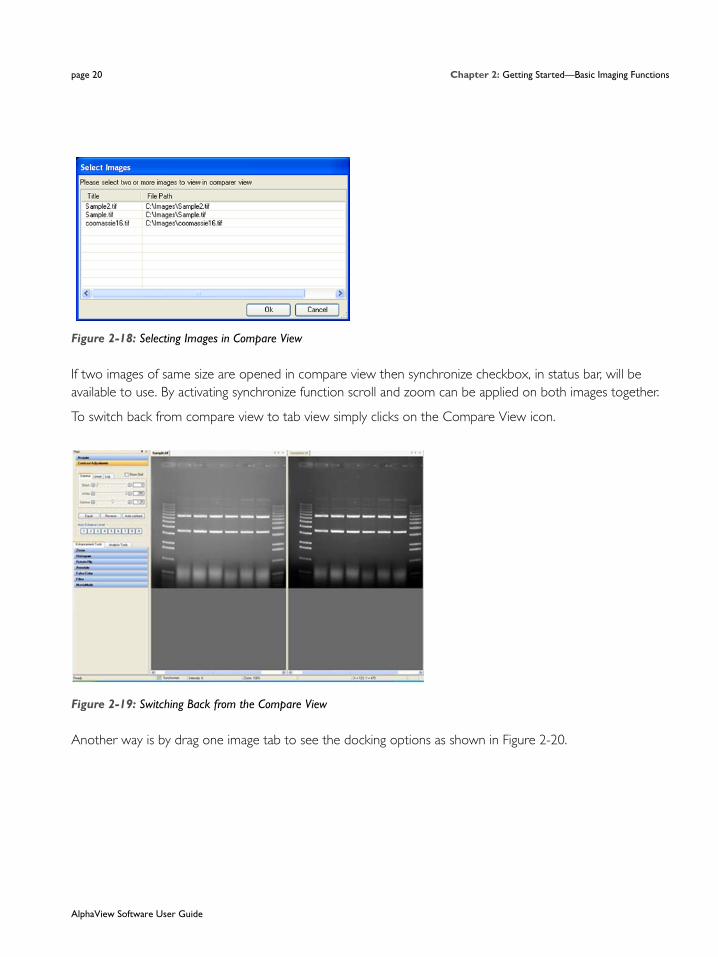
Figure 2-18: Selecting Images in Compare View
If two images of same size are opened in compare view then synchronize checkbox, in status bar, will be available to use. By activating synchronize function scroll and zoom can be applied on both images together.
To switch back from compare view to tab view simply clicks on the Compare View icon.
Figure 2-19: Switching Back from the Compare View
Another way is by drag one image tab to see the docking options as shown in Figure 2-20.
AlphaView Software User Guide

Imaging Tools page 21
Figure 2-20: How to Enter Compare View
After selecting appropriate place, when you drop the image tab, compare view will be opened.
Figure 2-21: Compare View
AlphaView Software User Guide

page 22 Chapter 2: Getting Started—Basic Imaging Functions
Tool Box
The Tool Box window contains an intuitive interface for performing all image enhancement and analysis functions.
Figure 2-22: Tool Box
The Enhancement Tools option contains the controls for enhancing and adjusting the image. This includes software filtering, false colors, zoom factors, and other unique features. The Analysis Tools contain the controls for quantitative analysis including gel smiling corrections, band matching, Lane Profile densitometry, multiplex band analysis, molecular weight calculations, colony counting, and arrays. Both the Enhancement Tools and the Analysis Tools are detailed in Chapter 4, “Image Enhancement Tools“ and Chapter 5, “Image Analysis Tools“, respectively.
Status Bar
The Status Bar is located on the bottom of the monitor and provides a real time display of the mouse cursor x, y position, the image zoom factor, and the grayscale intensity at the mouse cursor x, y position.
Figure 2-23: Status Bar
AlphaView Software User Guide
page 23
Chapter 3:
Drop-Down Menus
Chapter Overview• Main Menu
• File Menu
• Edit Menu
• Image Menu
• Setup Menu
• Overlay Menu
• Utilities Menu
• View Menu
• Window Menu
• Help Menu
AlphaView Software User Guide

page 24 Chapter 3: Drop-Down Menus
Main MenuAcross the top of the screen is a Windows menu bar containing several system operation functions. These include file saving and loading, edit, image, setup, overlay, file utilities, view, window and help functions.
Figure 3-1: AlphaView Drop-Down Menu Bar
File MenuUse this menu to save an image as a file, retrieve a previously saved image, select different printers, print an image, close an image or exit the software.
Figure 3-2: File Pull-Down Menu
File > Open Menu
This function opens the following image formats: .fcz, .png, .tif, .jpg and .bmp.
AlphaView Software User Guide

File Menu page 25
Figure 3-3: File > Open Dialog Box
Select Open from the File menu. The file type selection will default to show only .tif or .fcz files. To open other file formats, select the File Type box and select All image files:
Select the file of interest and click Open.
NOTE: FluorChem E and FluorChem M image files are provided in .fcz or .png formats only. Image files
from all other ProteinSimple FluorChem and AlphaImager systems are provided in .tif format.
AlphaView Software User Guide

page 26 Chapter 3: Drop-Down Menus
File > Save/Load Analysis
You can use Save/Load analysis feature from file drop-down menu, to save all your work and then load it back for later use.
NOTE: The load analysis menu item can only be accessed when the user opens any the analysis tools. If the image opened has an analysis saved, the item will be activated.
Figure 3-4: Save/Load Analysis Feature
File > Close Menu
This function closes the image currently displayed on the screen.
File Save, Save As, Save Modified, and Save All Menus
Save allows original images to be saved in several different formats. Save As allows images that have previously been saved to be saved in a different location or as a different file type without affecting the original image. Save Modified saves the image as a 8-bit color image with annotations burned into the image. Save All saves all images in .tif format only.
AlphaView has the ability to save files in several formats; see Figure 3-5.
AlphaView Software User Guide

File Menu page 27
Figure 3-5: File > Save As Dialog Box
Enter a new file name in the text box adjacent to the File Name prompt. Next, choose a file type from the Save As type list.
AlphaView will automatically give the appropriate 3-character extension. AlphaView will also create a file with the same base name and a .STP extension. This setup file saves information specific to this file, such as Black Level, White Level, Gamma Setting and 1D-Multi template placement. If the file is accessed later, these set-tings will be recalled.
File TypesTIFF is the default file format for AlphaView files. TIFF is an acronym for “tagged image file format” and was developed as a flexible and machine-independent graphic file format. Saving as a TIFF file will allow users to double-click TIFF files from Windows Explorer and automatically launch the application on any machine that has AlphaView loaded on it. Please refer to “Preferences” on page 39 for information on how to customize the default file type.
FCZ files are a proprietary zipped file format generated by FluorChem E and FluorChem M systems. Each file contains acquisition and user-entered image information along with a16-bit PNG file for the image data acquired for each channel. When FCZ files are opened in AlphaView software, this embedded PNG file opens automatically.
BMP, PNG, and JPG are additional graphic file formats which may be useful when saving an image for desktop publishing. These file formats can be imported directly into many Macintosh® and PC programs.
AlphaView Software User Guide

page 28 Chapter 3: Drop-Down Menus
NOTE: Do not use these formats to save images that will be analyzed later, since pixel data can be lost or altered when saving files in these formats.
NOTE: Not all file types can be saved as a 16-bit file. AlphaView software allows 8-bit TIFF images to be saved as BMP, JPG or PNG format and vice versa. 16-bit TIFF images can be converted into 8-bit TIFF, BMP, JPG or PNG format images.
Original versus Modified Files
An Original image file is one in which the data is saved in an unaltered form. This option should be selected if the image will be analyzed later. If the Black level, White level, or Gamma settings have been adjusted, the new values are saved but the pixel values are not altered. When this file is opened at a later time, AlphaView will display it with the values that were displayed when the image was saved, however, it is still possible to revert to the original raw image file by selecting Reset on the Tool Bar.
Annotation information cannot be saved with the Original image option. It can, however, be saved as an Overlay. Please refer to “Overlay” on page 32 for more information.
If the image was saved as an original file using an older system, some distortion may occur when viewing it in desktop publishing or word processing programs. If this occurs, save a copy of the image in the modified for-mat before importing it into another software package.
An image that is saved as a modified file permanently retains the changes to the image’s Black level, White level, and Gamma setting. Annotations and any filtering performed are also saved with the image, replacing original image information with the new information.
NOTE: If the image is saved as a Modified file it is converted to an 8-bit image.
This function sends the image to the default printer specified in Print Setup.
Printer Setup
This function displays a dialog box in which the settings for the parallel printer are specified. When all the pertinent printing preferences have been specified, click on the OK button. If you purchased a printer with AlphaView, this will be preset from the factory.
AlphaView Software User Guide
File Menu page 29
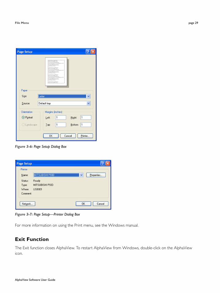
Figure 3-6: Page Setup Dialog Box
Figure 3-7: Page Setup—Printer Dialog Box
For more information on using the Print menu, see the Windows manual.
Exit Function
The Exit function closes AlphaView. To restart AlphaView from Windows, double-click on the AlphaView icon.
AlphaView Software User Guide

page 30 Chapter 3: Drop-Down Menus
Edit MenuThe Edit menu provides the ability to copy, crop, reset and remove any annotations or filters that have been added to the original image.
Figure 3-8: Edit Pull-Down Menu
Edit Activation
To activate the Copy and Crop functionality, place a check mark next to Edit Activation. This will turn the mouse cursor into a + sign that will allow you to highlight the region of interest for the image. After Edit Activation is highlighted, the desired area of interest is drawn using the mouse.
Figure 3-9: Ready to Crop or Copy
AlphaView Software User Guide

Image Menu page 31
Once this is completed, you can select either the Copy or Crop function in the Edit menu options.
Copy and Crop
Copy will copy the desired area of interest into the Windows Clipboard and allow you to paste into any desktop publishing package (i.e. Word, Excel, Adobe Photoshop, etc.).
Crop will display just the region of interest as the active window in the AlphaView interface.
Figure 3-10: AlphaView Interface—Sample Crop 1
Reset and Clear Options
The Reset option configures the Black, White, and Gamma settings to default settings. The Clear option removes any annotations that are present on the image.
Image MenuThe Image menu provides the ability to perform a variety of image processing functions.
AlphaView Software User Guide
page 32 Chapter 3: Drop-Down Menus
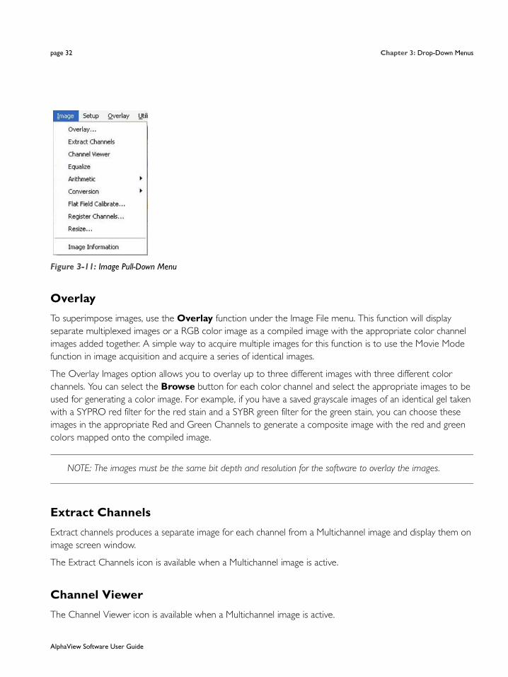
Figure 3-11: Image Pull-Down Menu
Overlay
To superimpose images, use the Overlay function under the Image File menu. This function will display separate multiplexed images or a RGB color image as a compiled image with the appropriate color channel images added together. A simple way to acquire multiple images for this function is to use the Movie Mode function in image acquisition and acquire a series of identical images.
The Overlay Images option allows you to overlay up to three different images with three different color channels. You can select the Browse button for each color channel and select the appropriate images to be used for generating a color image. For example, if you have a saved grayscale images of an identical gel taken with a SYPRO red filter for the red stain and a SYBR green filter for the green stain, you can choose these images in the appropriate Red and Green Channels to generate a composite image with the red and green colors mapped onto the compiled image.
NOTE: The images must be the same bit depth and resolution for the software to overlay the images.
Extract Channels
Extract channels produces a separate image for each channel from a Multichannel image and display them on image screen window.
The Extract Channels icon is available when a Multichannel image is active.
Channel Viewer
The Channel Viewer icon is available when a Multichannel image is active.
AlphaView Software User Guide
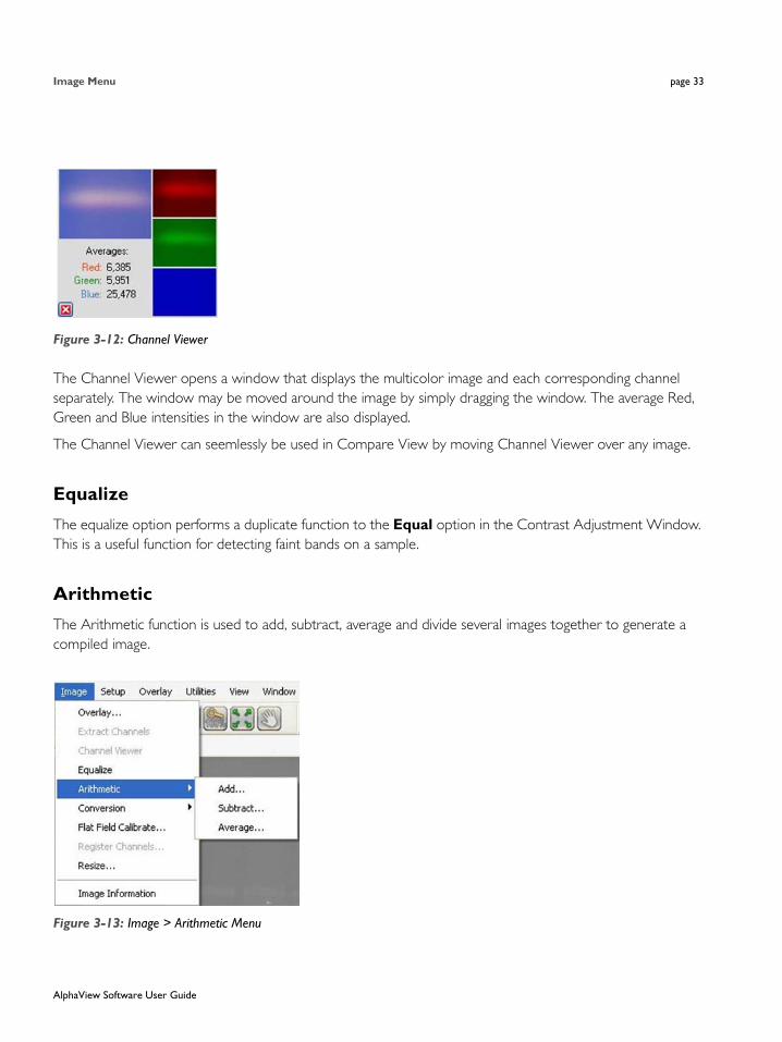
Image Menu page 33
Figure 3-12: Channel Viewer
The Channel Viewer opens a window that displays the multicolor image and each corresponding channel separately. The window may be moved around the image by simply dragging the window. The average Red, Green and Blue intensities in the window are also displayed.
The Channel Viewer can seemlessly be used in Compare View by moving Channel Viewer over any image.
Equalize
The equalize option performs a duplicate function to the Equal option in the Contrast Adjustment Window. This is a useful function for detecting faint bands on a sample.
Arithmetic
The Arithmetic function is used to add, subtract, average and divide several images together to generate a compiled image.
Figure 3-13: Image > Arithmetic Menu
AlphaView Software User Guide

page 34 Chapter 3: Drop-Down Menus
To average a set of images together open one of the images in the set and then select ‘Average a Set…’ under the Image pull-down menu. A prompt will appear allowing the user to select all of the images that for the set. It is possible to browse the directories looking on the network drives and removable media if necessary. Once all of the images have been selected click on the open button to finish the image set. The resulting image is an average of all of the images together. This is a useful function for extending the dynamic range on a set of sim-ilar images by allowing bright spots and faint spots to be seen on the same image.
The other functions are adding, subtracting and dividing images together. Adding together images is frequently used for colorimetric markers run together with chemiluminescent samples. Subtracting images is often used to remove noise from a sample by running dark images first and subtracting them out of the final image. The most common application for quotient is for those technical users who run their own flat field corrections. This can be done using the Flat Field Calibrate selection under the Image pull down menu which will be described in detail later in this section.
All three of these arithmetic functions are performed by opening the main image that will be adjusted. Next select the appropriate arithmetic function under the image pull down menu. Then select the image that is to be added, subtracted or divided from the original image and select open. The dialog box will disappear and the resultant image will appear.
NOTE: Images that have been arithmetically altered are ideal for publications and documentation, how-ever, they are strongly not recommended for analysis as the pixel values have been adjusted.
Conversion
Because AlphaView can generate 16-bit files, the conversion option is useful when an image is to be imported into a program that only accepts 8-bit images. Choosing this option will convert a 16-bit image into an 8-bit image.
A 48-bit color image can be converted into a 16 bit grayscale image by simply averaging the RGB values for each pixel.
AlphaView Software User Guide
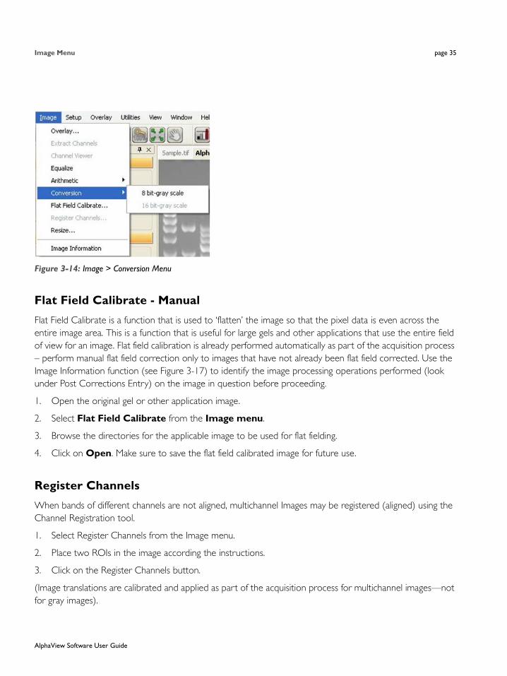
Image Menu page 35
Figure 3-14: Image > Conversion Menu
Flat Field Calibrate - Manual
Flat Field Calibrate is a function that is used to ‘flatten’ the image so that the pixel data is even across the entire image area. This is a function that is useful for large gels and other applications that use the entire field of view for an image. Flat field calibration is already performed automatically as part of the acquisition process – perform manual flat field correction only to images that have not already been flat field corrected. Use the Image Information function (see Figure 3-17) to identify the image processing operations performed (look under Post Corrections Entry) on the image in question before proceeding.
1. Open the original gel or other application image.
2. Select Flat Field Calibrate from the Image menu.
3. Browse the directories for the applicable image to be used for flat fielding.
4. Click on Open. Make sure to save the flat field calibrated image for future use.
Register Channels
When bands of different channels are not aligned, multichannel Images may be registered (aligned) using the Channel Registration tool.
1. Select Register Channels from the Image menu.
2. Place two ROIs in the image according the instructions.
3. Click on the Register Channels button.
(Image translations are calibrated and applied as part of the acquisition process for multichannel images—not for gray images).
AlphaView Software User Guide

page 36 Chapter 3: Drop-Down Menus
Figure 3-15: Channel Registration
Resize Image
The Resize function is to resize an image to a specific dimension for use in graphical presentations. You have the option to ‘Preserve aspect ratio’ to avoid image dimensional distortion, or you can deactivate this function and configure the image resolution to the desired width and height dimensions.
Figure 3-16: Resize Image Dialog Box
AlphaView Software User Guide

Setup Menu page 37
NOTE: It is recommended that you DO NOT perform quantitative analysis on resized images.
Image Information
The Image Information function provides a dialog box with all detailed image properties. To remove this dialog box from the screen, click OK.
Figure 3-17: Image Information Dialog Box
Setup MenuThis menu customizes the system settings by allowing users to save default parameter preferences and customize the software settings.
AlphaView Software User Guide

page 38 Chapter 3: Drop-Down Menus
Figure 3-18: Setup Pull-Down Menu
Print Info
Figure 3-19: Setup > Print Info Menu
When printing an image, basic image information is included on the print. This includes the exposure time, the Black level, White level, and Gamma setting, the date and time the image file was generated, an image ID number, and the name of the file to which the image is stored.
To print this information at the top of the print, choose Top from this menu. To print at the bottom of the print, choose Bottom.
NOTE: Printing image information at the top or bottom of a print may obscure a small portion of the image. To print the image with no information on it, choose Off.
AlphaView Software User Guide

Setup Menu page 39
Print Mode
AlphaView software provides custom printing options.
Figure 3-20: Setup > Print Mode Menu
Printing can be achieved in three different methods:
• Full Image—Prints the original image. Does not print zoomed images or images overlaid with data screens.
• Screen Dump—Prints the imaging area. Well suited for printing images overlaid with data screens and/or graphs, zoomed images, etc.
• Image Window—Prints the highlighted window.
Print Date
Under the Setup menu there is a selection labeled “Print Info”. This allows the user to change the format in which the date is printed. The choices are MM/DD/YYYY and DD/MM/YYYY.
Preferences
In order to change the preferences of the system, you will need to log in. This is enforced only on data altering tool tabs such as image acquire, cabinet settings, and auto enhancement. To login, enter the word master for both the user name and password.
Figure 3-21: User Login Dialog Box
AlphaView Software User Guide

page 40 Chapter 3: Drop-Down Menus
There are five tabs in the Preferences menu:
NOTE: The Image Acquire and Cabinet Settings tabs are not active the AlphaView Stand Alone software version.
• General—Configures prompts and file saving/opening formats.
Figure 3-22: Preferences—General Tab
• Auto Enhancements—Used to customize the Auto Enhance Levels located in the Image Enhancement tool box.
AlphaView Software User Guide

Setup Menu page 41
Figure 3-23: Preferences—Auto Enhancement Tab
To make changes to the preferences, select your change by typing in a new value or select/de-select the appropriate box with a check mark and then select apply. Some settings may require that the software be re-started for the change to take effect.
• Analysis Tools—Used to show/hide additional image analysis tools. Any change in the settings will require software be re-started for the change to take effect.
Figure 3-24: Preferences—Analysis Tools Tab
AlphaView Software User Guide

page 42 Chapter 3: Drop-Down Menus
Overlay MenuThe Overlay menu provides a means of saving and retrieving annotation overlays. This is especially useful when a standard gel format is run repeatedly. Lane numbers, molecular weight marker sizes, and other pertinent information can be stored as an Overlay file and retrieved at a later date. This eliminates the need to re-enter the information each time a new image is captured.
Figure 3-25: Overlay Pull-Down Menu
An overlay is any set of annotations (text, boxes, arrows, etc.) that have been drawn on the image. They can be saved as a group and opened later. If repetitive samples are being imaged, an overlay eliminates the need to re-enter the same information (such as lane numbers, standard sizes, etc.) continually.
Load Overlay
The Load Overlay function allows Overlay files to be retrieved and applied to the image currently displayed.
Opening an Overlay after an image has been captured places the annotations on top of the image. They can be stored as part of the image by saving the file as a modified file. Please refer to “File Save, Save As, Save Modified, and Save All Menus” on page 26 for more information.
Select the name of the file to be loaded. (If necessary, change the directory or drive.) The file name is then highlighted in the list and appears in the text box below the Filename prompt.
Once the file has been selected, click on the OK button to load the file. (Alternatively, double-click on the file name.) The dialog box disappears and the annotations in the selected file appear on the image.
To dismiss the dialog box without loading annotations, click on the CANCEL button.
Save Overlay
Once annotations have been made, select Overlay > Save Overlay.
AlphaView Software User Guide

Utilities Menu page 43
Figure 3-26: Save Overlay File Selection Dialog Box
Enter a new file name in the text box below the File Name prompt. AlphaView will automatically give the appropriate 3-character extension.
The current directory is the one in which the new overlay file will be saved. If necessary, change the directory or drive as described in Section 3.1.
Once a name has been entered and the appropriate directory has been accessed, click the SAVE button to save the overlay file.
Show Annotation
To displays or hides annotations in Analysis modules.
Utilities MenuA number of functions are now handled by Windows programs. To access many of these programs while in AlphaView, open the Utilities menu and select the program of choice.
AlphaView Software User Guide

page 44 Chapter 3: Drop-Down Menus
Figure 3-27: Utilities Pull-Down Menu
Notepad
The Notepad is a blank screen that allows the user to make notes about the experiment and save them as an ASCII file. The Notepad is useful for saving any imaging comments or experimental conditions with the saved image for future reference.
Figure 3-28: Notepad Display Window
Explorer
Windows Explorer allows access to files and other information saved on the local machine or the network, if applicable.
AlphaView Software User Guide

View Menu page 45
Figure 3-29: Windows Explorer Window
View MenuThe View menu provides the ability to control the display of the on-screen control tools as well as provide image enhancement abilities.
Figure 3-30: View Pull-Down Menu
AlphaView Software User Guide

page 46 Chapter 3: Drop-Down Menus
Default Tools Position
Four (4) main control windows exist within AlphaView: Tool Bar, Contrast Adjustment, Tool Box, and Status Bar :
Figure 3-31: Tool Bar
Figure 3-32: Contrast Adjustments Window
Figure 3-33: ToolBox Window
Figure 3-34: Status Bar
AlphaView Software User Guide

Window Menu page 47
These control windows automatically open when AlphaView is launched for additional ease of use and to generate a common ‘look and feel’. Since these items are ‘floating’ tools, you can click on Default Tools Position to move all tools to the default locations for more intuitive operation. Lastly, except for the status bar, it is possible to select and move any of the other windows to a custom location.
Zoom Functions
Additional options provide the ability to Zoom In and Zoom Out on the image, Zoom to 1X and to Fit to Screen.
NOTE: Zoom In and Zoom Out are duplicate functions for the Zoom In and Zoom Out icons in the ToolBar and the Zoom options in the Enhancement Tools.
Window MenuThe Window menu provides the ability to navigate from one image window to next image window. It also allows user to close all documents.
Figure 3-35: Window Pull-Down Menu
AlphaView Software User Guide

page 48 Chapter 3: Drop-Down Menus
Help Menu
Figure 3-36: Help Pull-Down Menu
Complete instructions on how to use the software along with detailed explanations of all features are avail-able from the AlphaView Help option of the Help menu.
To display system information, select the About option in the Help menu. This button accesses a pop-up box (see Figure 3-37), which shows the system serial number and software version number. Use this information when contacting ProteinSimple for technical support, software upgrades, etc.
Figure 3-37: AlphaView—About Help Display
To close the box, click on the OK button.
AlphaView Software User Guide

page 49
Chapter 4:
Image Enhancement Tools
Chapter Overview• Tool Box Enhancement Tab
• Zoom
• Histogram
• Rotate-Flip
• Annotate
• False Color
• Filter
• Movie Mode
AlphaView Software User Guide

page 50 Chapter 4: Image Enhancement Tools
Tool Box Enhancement TabImage enhancement tools are contained within the Tool Box as indicated. This tool set allows the user to zoom the image, rotate-flip the image, show the image histogram, perform automatic image enhancement, annotate on the image, display false colors, apply software filters, and activate the Movie function.
NOTE: Many image enhancement tools do not function with multichannel images.
Figure 4-1: Tool Box
Zoom
Figure 4-2: Zoom Tool
The Zoom tool function magnifies an image, making details easier to see, and allows movement around the magnified image.
AlphaView Software User Guide
Histogram page 51
An image can be displayed ¼x, ½x, 1x, 2x, 4x, or 8x larger than the original display by clicking on the appropriate buttons. To return to the original magnification, click on the 1X button.
When an image is magnified, only part of it can be displayed on the screen at any one time. To see different parts of the magnified image, use the green Pan Control box. The outer box shows a thumbnail of the entire image while the inner green box represents the portion currently displayed on the screen.
To view different regions of a magnified image, move the cursor into the inner box. Click and hold down the left mouse button. The cursor changes to a hand; use it to drag the green box until the desired region of the image appears on the screen.
Alternatively, use the scroll bars in the image window to move the image up or down, and left or right.
On-screen Zoom tools are also available located on the main Tool Bar. This function duplicates the Zoom tool in the Tool Box, and also allows for Image Drag to easily pan the image during any analysis functions located in “Zoom” on page 50 (in the Analysis Tools option).
Image Drag icon in ToolBar
Zoom Icons in ToolBar
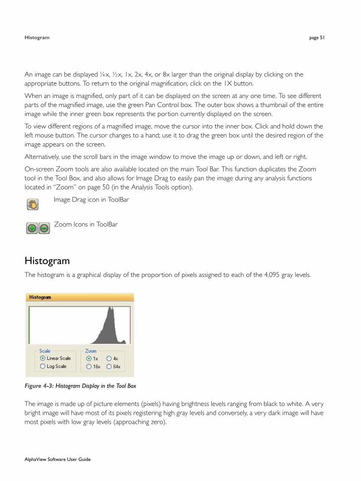
HistogramThe histogram is a graphical display of the proportion of pixels assigned to each of the 4,095 gray levels.
Figure 4-3: Histogram Display in the Tool Box
The image is made up of picture elements (pixels) having brightness levels ranging from black to white. A very bright image will have most of its pixels registering high gray levels and conversely, a very dark image will have most pixels with low gray levels (approaching zero).
AlphaView Software User Guide

page 52 Chapter 4: Image Enhancement Tools
The histogram is displayed in the lower left corner of the screen, below the image window. The horizontal axis represents the gray scale range: black at the left end and white at the right end, with levels of gray in between. The number of pixels registering a particular gray level determines the height of each bar along the axis.
A Coomassie blue-stained protein gel visualized with a white light box has a histogram reflecting mostly bright pixels:
Figure 4-4: Histogram of a Typical Coomassie Gel
Most of the pixels are found in the light portion of this histogram. The dark bands represent a small number of pixels and include a variety of gray values, and therefore do not show up as a single peak.
The histogram function is particularly useful to verify that an image spans the maximum range of gray levels. When an image is to be used for analysis, it is especially important that the gray level range be as large as possible. If an image does not include most of the gray levels, we recommend repeating the image capturing process.
AlphaView Software User Guide
Rotate-Flip page 53
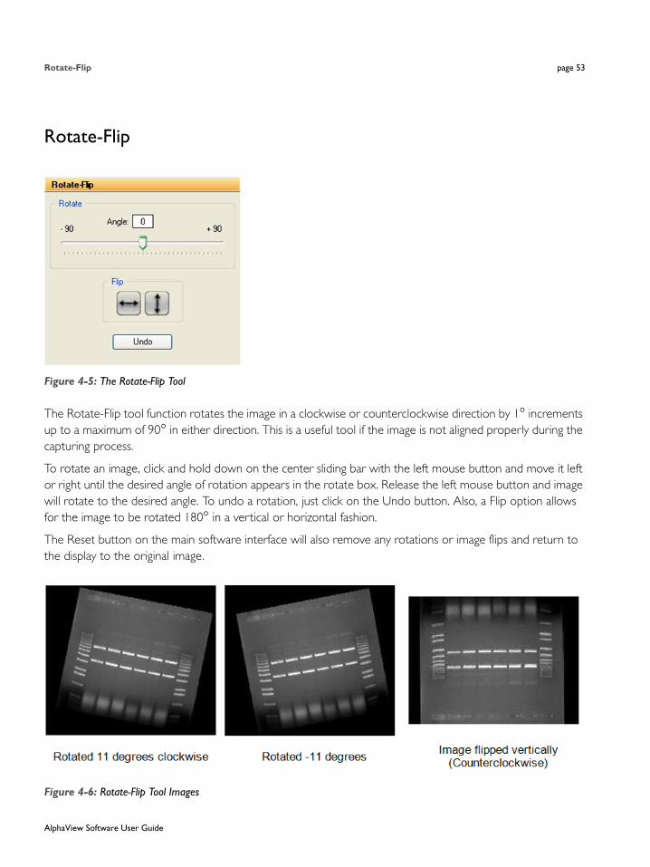
Rotate-Flip
Figure 4-5: The Rotate-Flip Tool
The Rotate-Flip tool function rotates the image in a clockwise or counterclockwise direction by 1° increments up to a maximum of 90° in either direction. This is a useful tool if the image is not aligned properly during the capturing process.
To rotate an image, click and hold down on the center sliding bar with the left mouse button and move it left or right until the desired angle of rotation appears in the rotate box. Release the left mouse button and image will rotate to the desired angle. To undo a rotation, just click on the Undo button. Also, a Flip option allows for the image to be rotated 180° in a vertical or horizontal fashion.
The Reset button on the main software interface will also remove any rotations or image flips and return to the display to the original image.
Figure 4-6: Rotate-Flip Tool Images
AlphaView Software User Guide

page 54 Chapter 4: Image Enhancement Tools
Figure 4-7: Rotate-Flip Tool Controls
AnnotateThe annotation tools include a number of different options for adding text (including Greek symbols), drawing arrows and otherwise marking an image.
NOTE: These tools are for annotation only. For information on drawing objects for quantitation purposes, see Chapter 5, “Image Analysis Tools“.
AlphaView Software User Guide
Annotate page 55
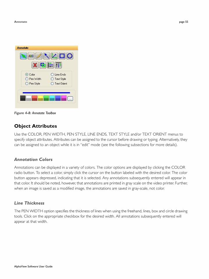
Figure 4-8: Annotate Toolbox
Object Attributes
Use the COLOR, PEN WIDTH, PEN STYLE, LINE ENDS, TEXT STYLE and/or TEXT ORIENT menus to specify object attributes. Attributes can be assigned to the cursor before drawing or typing. Alternatively, they can be assigned to an object while it is in “edit” mode (see the following subsections for more details).
Annotation Colors
Annotations can be displayed in a variety of colors. The color options are displayed by clicking the COLOR radio button. To select a color, simply click the cursor on the button labeled with the desired color. The color button appears depressed, indicating that it is selected. Any annotations subsequently entered will appear in that color. It should be noted, however, that annotations are printed in gray scale on the video printer. Further, when an image is saved as a modified image, the annotations are saved in gray-scale, not color.
Line Thickness
The PEN WIDTH option specifies the thickness of lines when using the freehand, lines, box and circle drawing tools. Click on the appropriate checkbox for the desired width. All annotations subsequently entered will appear at that width.
AlphaView Software User Guide

page 56 Chapter 4: Image Enhancement Tools
Figure 4-9: Pen Width Selection Tools
Line Types
The PEN STYLE option specifies the style of lines when using the freehand, lines, box and circle drawing tools. Click on the appropriate checkbox for the desired style. All annotations subsequently entered will appear in that style.
NOTE: These pen styles only work with a thin line (see the “Line Thickness” section).
Figure 4-10: Pen Style Selection Tools
AlphaView Software User Guide

Annotate page 57
Arrows and Straight LinesThe LINE ENDS option specifies the style of the ends of straight lines (no arrow, single arrow or double arrow). Click on the appropriate checkbox for the desired style.
NOTE: These line ends work with any line thickness.
Figure 4-11: Line Ends Selection Tools
Text Background and Font
The TEXT STYLE option specifies the style of text. Click on the appropriate checkbox to show text with or without a background. An opaque background is useful if annotations will be made on an image that has wide variations in gray scale. By using an opaque background, text will not be “lost” in the background of the image.
AlphaView Software User Guide

page 58 Chapter 4: Image Enhancement Tools
Figure 4-12: Text Style Selection Tools
This is also the window in which specific font is chosen. When the Set Font button is depressed, a selection box appears, from which text style can be chosen.
Figure 4-13: Font Selection Dialog Box
NOTE: To choose Greek symbols (such as α, β, λ, π, and θ) choose the Symbol font: a b c d e f g h i j k l m n o p q r s t u v w x y zαβχδεφγηιϕκλμνοπθρστυϖωξψζ
AlphaView Software User Guide

Annotate page 59
Text Orientation
In the TEXT ORIENT window, select whether text should be oriented vertically, horizontally, or at an angle (in 15° increments).
Figure 4-14: Text Orient Selection Tools
NOTE: Only rotate fonts that are True Type (indicated by TT in front of the name); other fonts (such as Courier and Fixedsys) do not re-scale properly, giving unpredictable results.
Drawing Tools
Once the object attributes have been defined, click the cursor on any of the drawing tool buttons to assign the function associated with that button to the mouse. The cursor will change from an arrow to a cross, indicating that AlphaView is in “drawing” mode.
After selecting a drawing tool, move the cursor to the correct position on the image to begin drawing. Press and hold the left mouse button and move the mouse to the end point of the object to be drawn. Release the left button, and the object should appear.
Boxes will appear at the corners of the new object and the cursor will revert to an arrow, indicating that AlphaView is now in “edit” mode. At this point, the object can be resized or repositioned. The color, pen thickness, line type, etc. can also be changed, simply by clicking on the desired choice (as described in “Object Attributes,” starting on page 55).
AlphaView Software User Guide

page 60 Chapter 4: Image Enhancement Tools
To draw another object, click the right mouse button to return to “draw” mode, or click on one of the drawing tool icons.
Table 4-1: Drawing Tool Icon Descriptions
Icon Description
The selection tool, allows the user to select all drawing for further operations, such as vertical alignment.
The button labeled with an "ABC" adds text to the image. Place the cursor at the location on the image where the left edge of the text should appear. Click the left mouse button and begin typing. To place another piece of text, click where it should be placed. Once all text is entered, click on the right mouse button. To edit text, double-click on it. An edit window will appear, in which changes can be made. To change fonts, see “Text Background and Font,” starting on page 57.
The button labeled with a pencil icon allows the user to draw lines freehand. After clicking on the pencil, move the cursor to the correct position on the image to begin drawing. Press and hold the left mouse button. Using the mouse, move the cursor as if it were a pencil. When finished drawing, release the mouse button.
The button labeled with a diagonal line and arrow, draws arrows and straight lines. After clicking on the button, move the cursor to the position on the image where the line should begin. Press and hold the left mouse button. Using the mouse, move the cursor to the other end point of the line then release the mouse button. The arrow can be adjusted by clicking on one of the boxes at the end (the other will serve as an anchor point) or by clicking in the middle to drag the entire arrow.
The button labeled with angles and arrows on its side is a line drawing tool, very similar to the one described above. The significant difference is that this tool limits the angle that the line can be drawn to increments of 45°.
The button labeled with a square draws a rectangle or square of any size on the image. After clicking on the button, move the cursor to the position that should correspond to one of the cor-ners of the rectangle. Press and hold the left mouse button. Using the mouse, move the cursor to enlarge the rectangle. When it reaches the desired size, release the left mouse button.
The button labeled with a circle draws a circle of any size. After clicking on the button, move the cursor to the position on the image where the circle should be started. Press and hold the left mouse button. Using the mouse, move the cursor to enlarge the circle. When the circle reaches the desired size, release the left mouse button.
AlphaView Software User Guide

Annotate page 61
Hint: to draw a perfect circle around a portion of an image, first visualize a square surrounding the area of interest. Position the mouse in the upper left hand corner of the square. Click and drag the mouse down across the area of interest at a 45° angle until the circle encloses the area of interest.
Sample Annotations
Figure 4-15: Sample Annotations
Annotated image showing: freehand drawings, lines with various characteristics, circles, squares, text with various characteristics
Editing Tools
When the cursor is in “edit” mode, it can be clicked on an object to select it.
NOTE: The cursor can be toggled between “edit” and “drawing” modes by clicking the right mouse button.
When an object is selected, small square boxes appear at the corners. Selected objects can be resized, copied, deleted or moved:
• To resize an object, click on one of the gray boxes at the corners of its perimeter and drag the box until the object reaches the desired size.
AlphaView Software User Guide

page 62 Chapter 4: Image Enhancement Tools
• To copy an object, use the Copy tool.
• To delete an object, use the Cut tool or the Eraser.
• To move an object, click within its boundary and drag it into the desired location.
To select more than one object, outline them with the mouse; any objects that fall completely within the outline drawn will be selected.
NOTE: The entire object must be enclosed by the cursor’s movement in order to be selected.
Figure 4-16: A Selected Object
AlphaView Software User Guide

False Color page 63
Table 4-2: Editing Tools
False ColorThese tools consist of eleven pre-defined color palettes that can be applied to an image. To select a palette, simply click on one of the four buttons labeled Gray Palette, High-Low, Next or Previous.
Icon Description
Once an object or group of objects has been selected, clicking on the Cut tool deletes it from the image.
The Copy tool makes an exact copy of the selected object. The new object becomes the selected object, and can be repositioned by placing the cursor within the object’s boundary and moving it to the desired location.
The Horizontal Alignment tool aligns annotations in a straight horizontal line. This is especially useful for labeling lanes, etc. To use this tool, draw text on the image, select it, click the Horizontal Alignment tool, then deselect the text. The text will now be aligned in a straight line across the image.
The Vertical Alignment tool aligns annotations in a straight vertical line. This is especially useful for labeling markers, etc. To use this tool, draw text on the image, select it, click the Vertical Align-ment tool, then deselect the text. The text will now be aligned in a straight line down the image.
AlphaView Software User Guide

page 64 Chapter 4: Image Enhancement Tools
Figure 4-17: False Color Selection Box
When a palette is selected, its range of colors is displayed to the left of the palette buttons and automatically applied to the image. To apply a different palette to the image, click Next or Previous.
NOTE: Changes in Black level, White level, and Gamma setting can alter the effect of each of the palettes, and can enhance the results produced.
Gray Scale (Palette 0)
This is the default or standard gray scale, consisting of different gray levels, ranging from black to white.
High–Low (Palette 1)
This is a modified gray scale palette in which black is replaced with green, and white is replaced with red. Over- and under-exposed areas of the image are thus shown as green or red, while areas within the linear range of the CCD chip are shown in gray scale. The Saturation Palette is especially useful during quantitation, as areas outside the linear range of the instrument do not give accurate quantitative information. This palette allows the user to avoid those areas during quantitative analysis.
This palette can also be accessed by clicking the Show Saturation checkbox in the Camera Setup and Preview function (accessible by clicking on the Camera icon in the Tool Bar window)
Other Palettes
These are color substitution palettes in which the gray levels are translated into different color ranges. These palettes can be useful to help distinguish features and highlight details on an image.
AlphaView Software User Guide

False Color page 65
• Palette 2 maps the gray scale levels to a red/green/blue palette. Values of 0 are mapped to red; saturated to blue, and values in between to green.
• Palette 3 maps the gray scale levels to a red/green/blue palette. Values of 0 are mapped to blue; saturated to green, and values in between to red.
• Palette 4 maps the gray scale levels to a red/green/blue palette. Values of 0 are mapped to green; saturated to red, and values in between to blue.
• Palette 5 maps the gray scale levels to a cyan/magenta/yellow palette. Values of 0 are mapped to cyan; saturated to yellow, and values in between to magenta.
• Palette 6 maps the gray scale levels to a cyan/magenta/yellow palette. Values of 0 are mapped to yellow; saturated to magenta, and values in between to cyan.
• Palette 7 maps the gray scale levels to a cyan/magenta/yellow palette. Values of 0 are mapped to magenta; saturated to cyan, and values in between to yellow.
• Palette 8 maps the gray scale levels to shades of red palette. This palette may be useful when viewing red color images.
• Palette 9 maps the gray scale levels to a red palette. Values of 0 are mapped to dark red; saturated to white, and values in between to shades of red.
• Palette 10 maps the gray scale levels to shades of blue palette. This palette may be useful when viewing blue color images.
• Palette 11 maps the gray scale levels to a blue palette. Values of 0 are mapped to dark blue; saturated to white, and values in between to shades of blue. This palette may be useful when printing an image of a Coomassie-stained protein gel onto a color printer.
• Palette 12 maps the gray scale levels to shades of green palette. This palette may be useful when viewing green color images.
• Palette 13 maps the gray scale levels to a green palette. Values of 0 are mapped to dark green; saturated to white, and values in between to shades of green. This palette may be useful when printing an image of a SYBR Green I-stained protein gel onto a color printer.
• Palette 14 maps the gray scale levels to an orange palette. Values of 0 are mapped to dark orange; saturated to white, and values in between to shades of orange. This palette may be useful when printing an image of an EtBr-stained gel onto a color printer.
AlphaView Software User Guide

page 66 Chapter 4: Image Enhancement Tools
Filter
Figure 4-18: Filters Toolbox with 3-D (Contour) Selected
AlphaView includes a variety of enhancement filters that can improve the appearance of an image. Some filters sharpen detail, others smooth and reduce random noise. Still others help visualize edges and separate closely spaced bands or objects. Depending upon the unique characteristics of an image, the results of each filtering operation vary. Assess the characteristics of the image and then select the filter designed to minimize its imperfections.
When an image is filtered, the original image information is replaced with the results of the filtering operation. As a result, the original image information is altered. To avoid losing the original image, save it as an original TIFF file before applying a filter.
When the FILTERS button is selected, a pop-up box appears. If the desired filter is not shown, choose MORE to display more filters. One or many filters can be applied to a single image.
Figure 4-19: Filters Toolbox with Sharpen Highlighted
AlphaView Software User Guide

Filter page 67
Figure 4-20: Filters Toolbox with More Selected
General Information
To enhance an image, filters change the value assigned to each pixel. The new value assigned to a pixel is determined based on the values of the other pixels in its local vicinity (or “neighborhood”). The neighborhood is a two-dimensional matrix of pixel values, where each dimension has an odd number of elements. The “pixel of interest” is the one at the center of the neighborhood. This is the pixel whose old value is being replaced with a new one as the result of the filtering algorithm.
The pixels in a neighborhood provide information about the brightness trend. This information is important to the filtering process. The brightness trend is also referred to as the “spatial frequency.” Images with high spatial frequency content contain large, closely spaced changes in pixel values. For example, on a black and white checkerboard, the smaller the squares, the higher the frequency content.
Images with low spatial frequency content (for example, images of clouds) contain large areas of slowly changing pixel values.
Most of the filter options available (with the exception of the Noise filters) use a weighted summation process to determine the value assigned to the pixel of interest. Each pixel in a 3x3 neighborhood is multiplied by a “convolution kernel” having the same dimensions. The resulting sum is assigned to the pixel of interest.
AlphaView Software User Guide

page 68 Chapter 4: Image Enhancement Tools
Each element of the convolution kernel is a weighting factor, also called a “convolution coefficient.” The size and arrangement of these weighting factors determine the type of transformation the image will undergo. Changing a weighting factor influences the overall sum and, therefore, affects the value given to the pixel of interest.
Sharpening Filters
These filters can increase image sharpness and provide edge enhancement. However image noise may be enhanced as well. These filters accentuate the high-frequency details of an image while leaving the low-frequency content intact. High frequency portions of the image get brighter while low frequency portions become black.
Sharpen level 9 (high) has the largest effect on the image. Sharpen level 5 has an intermediate effect. Sharpen 1 (low) has the most subtle effect on the image. 9 different sharpening levels are available for optimization of the image.
Noise Filters
This filtering process uses the values of the pixels contained in the area surrounding a pixel to determine the new value given to the pixel of interest. The noise filter sorts the pixels in the neighborhood into ascending order and picks the middle or median pixel value as the new value for the pixel of interest. Three levels of noise reduction are available.
Despeckle Filters
The despeckle filter is a type of smoothing filter based on data rejection. Pixels in the neighborhood (usually the adjacent pixels) are used as a data set upon which the average and standard deviation of the set are calculated. If the pixel of interest (the center of the neighborhood) is different from the neighborhood average (either greater or lesser) by a threshold (a multiple of the standard deviation) it is replaced by the average value.
The effect of the filter is to “smooth” pixels that are much different from their neighbors. Artifacts such as hot pixels, cosmic rays etc. are commonly rejected by this type of filter. The filter strength is controlled by the threshold factor. For large factors very little data is rejected as only very large deviations are required for rejection, where as, low thresholds result in more smoothing. (For example, setting #1 results in outliers of 1 standard deviation greater or lesser than the neighborhood average to be corrected for, setting #2 results in outliers of 2.5 standard deviations to be corrected for and setting #3 results in outliers of 5 standard devia-tions to be corrected for.)
These filters are particularly effective in eliminating random noise contained in an image and produce less blurring than the noise filters.
AlphaView Software User Guide

Filter page 69
3-D (Contour) Filters
These filters are particularly useful for visualizing faint bands. They produce a “3-D” effect, defining edges and making details easier to see.
3-D level 9 (high) has the largest effect on the image. 3-D level 5 has an intermediate effect 3-D level 1 (low) has the least effect on the image. Nine different 3-D levels are available for optimization of the image.
In addition, 3-D allows the user to control the ‘direction’ of the 3-D shadowing effect. Once the level is refined, just click on a direction arrow to visualize the shadowing adjustment. The default shadow direction is in the lower right hand corner direction and 9 different directions are available.
Figure 4-21: 3D Image Examples
Figure 4-22: 3D Image Controls
AlphaView Software User Guide

page 70 Chapter 4: Image Enhancement Tools
Smoothing Filters
These filters are very useful for reducing the visual noise present in an image. When a smoothing filter is applied to an image, rapid changes in intensity are averaged out with the remaining pixels in the neighborhood, thereby decreasing the high frequency content. The visual result is a slight smoothing of the image because sharp pixel transitions are averaged with their surroundings.
Smooth High has the largest effect on the image. Smooth Med has an intermediate effect. Smooth Low has the most subtle effect on the image.
Edge Filters
These filters use Laplacian enhancement to highlight edges, regardless of direction. All edge-enhancement operations attenuate the low frequencies of the image. Regions of constant intensity or linearly increasing intensity become black as a result of these transformations, and regions of rapidly changing intensity values are highlighted.
NOTE: The White level may need to be adjusted after using the Edge filters in order to see the result of this filtering process.
Horizontal Edge Filter
This filter brightens horizontal edges. This can be useful in pinpointing bands on a gel. The horizontal edge filter (Horz. Edge) enhances image edges by shifting an image vertically by one pixel and then subtracting the shifted image from the original. In an area of constant pixel intensity, the subtraction yields black pixel values. At an edge, which is an area with large changes in intensity, the subtraction yields light-colored pixel values. The larger the difference in intensities, the lighter the resultant pixels.
NOTE: After applying the horizontal edge filter the entire image may appear black, and might require reducing the White level in order to better visualize the results.
Vertical Edge Filter
This filter (Vert. Edge) brightens vertical edges using the approach described for the horizontal edge filter (see above), except that the image is shifted horizontally before the shifted image is subtracted from the original. In this case, the vertical edges produce light-colored pixel values. As in the horizontal edge filter, it may be nec-essary to adjust the White level in order to better visualize the results of this filtering process.
AlphaView Software User Guide

Movie Mode page 71
Custom Filter
This function allows the use of customized filters. Using the weighting factors of the other filters as a frame of reference, experiment with new weighting factor values.
Undo Button
The upper right button is labeled Undo. This reverses the last filtering process applied to an image. To revert the image to its original state after multiple filters have been applied, press the Reset button on the main interface.
Examples of Filter Results
Figure 4-23: Examples of Filter Results
Movie ModeTo open and play existing movies, click on the Movie Mode tab in the Enhancement Tools.
AlphaView Software User Guide

page 72 Chapter 4: Image Enhancement Tools
Figure 4-24: Movie Mode In the Enhancement Tools
Click the Open button to open and play a previously recorded movie. To record a movie, click on the Record button. This will launch the Camera Setup and Preview window.
AlphaView Software User Guide

page 73
Chapter 5:
Image Analysis Tools
Chapter Overview• Tool Box Analysis Tools Tab
• Molecular Weight Determination
• Colony Count
• Multiplex Band Analysis
• Lane Profile
• Additional Analysis Tools
AlphaView Software User Guide

page 74 Chapter 5: Image Analysis Tools
Tool Box Analysis Tools TabDefault image analysis tools are contained within the Tool Box as indicated. This tool set allows the user to perform molecular weight determinations, automatic counting of colonies and cells, multiplex band analysis and lane profile densitometry.
Figure 5-1: Default Analysis Tools in the ToolBox
Molecular Weight DeterminationThe Molecular Weight button (in Tool Box, Analysis Tools) opens a set of tools for entering the values of known molecular weight markers and determining the molecular weights of unknown bands on the image. When the Molecular Weight button is selected, a function box appears in the area to the lower left of the screen, and a data box appears on the image. (If the data window obscures part of the image containing bands of interest, it can be moved.)
AlphaView Software User Guide
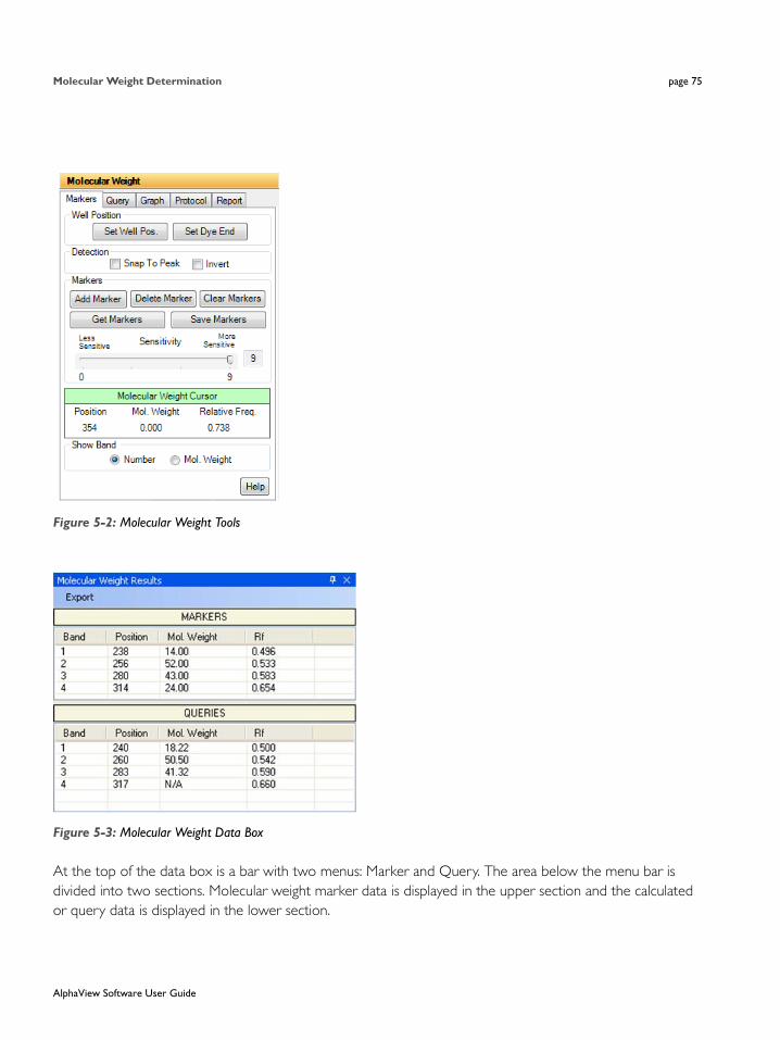
Molecular Weight Determination page 75
Figure 5-2: Molecular Weight Tools
Figure 5-3: Molecular Weight Data Box
At the top of the data box is a bar with two menus: Marker and Query. The area below the menu bar is divided into two sections. Molecular weight marker data is displayed in the upper section and the calculated or query data is displayed in the lower section.
AlphaView Software User Guide

page 76 Chapter 5: Image Analysis Tools
Entering Known Molecular Weights for Markers
An unlimited number of molecular weight standards can be defined, either all in one lane, or in multiple lanes. To input markers, open the Marker menu and select Add Marker.
NOTE: To enter standards from previously-saved files, see “Applying a Set of Saved Markers” on page 79.
Notice that the cursor flashes and has a short, horizontal line associated with it. Move the cursor to the lane containing the molecular weight standards. Beginning at the top of the lane, position the cursor so the horizontal line is aligned with the band.
If the Snap to Peak function has been activated, the cursor jumps to the highest pixel value in the band as the cursor approaches it. If bands are so tightly spaced that the line is not coinciding with the band, turn off Snap to Peak and place the marker on the band manually.
When the horizontal line is positioned correctly, click the left mouse button. A dialog box appears requesting the band's molecular weight. Using the numeric keypad in the dialog box (or the numbers on the keyboard), enter the known molecular weight. Alternatively, enter the value using the keyboard.
After entering the molecular weight, press either the OK button in the dialog box (or the <Enter> key on the keyboard). The dialog box disappears, the number of the band appears on the image, and the band's data is added to the Markers section of the data box. The horizontal red line remains, indicating that the cursor is ready to select the next band as described above.
After entering the value for the last marker, click the Add Markers Complete button instead of OK. This will deactivate the value-entering function and will return the cursor to its normal mode. (To reactivate the value-entering function, select Add Marker from the menu again, or click the right mouse button.)
The Molecular Weight Data Box
The data box is located near the top of the image. Initially, no values are displayed in the data box. When a molecular weight value is assigned to a band, the following information is displayed in the data box:
• Band numbers are assigned beginning with the first band, continuing in the order selected.
• The position corresponds to the band's location along the y-axis, ranging from 0 to 1030.
• The value displayed under the Molecular Weight. heading is the molecular weight value entered for a known and or the value calculated for an unknown band.
• The Rf value for each band is also displayed. Unless otherwise specified, AlphaView assumes the origin (Rf value = 0.00) is located at the top of the screen, and dye front (Rf value = 1.00) is at the bottom of the screen. Using these points as a frame of reference, AlphaView calculates Rf values for the interme-diate bands.
AlphaView Software User Guide

Molecular Weight Determination page 77
Figure 5-4: Molecular Weight Marker and Query Data
If the data box obscures part of the image, it can be resized or moved using Windows functions, or it can be hidden using the Hide Data checkbox.
Repositioning and Deleting Markers
Marker band indicators can be repositioned simply by positioning the cursor, clicking, and dragging the line to the desired location.
To delete a molecular weight marker, point the cursor at the appropriate marker band and click the left mouse button. This highlights the band in question by putting a red box around it. (Alternatively, clicking in the data table highlights the marker’s information and selects the band on the image.)
Click on the Delete Marker function in the Marker menu. The marker is deleted, as is the band's data in the marker data table. Markers entered after the deleted bands are renumbered on the image and the data table.
To delete all the markers and start over, select the Clear Markers function in the Marker menu.
Determining Molecular Weights of Unknown Bands
After marker values are entered, the molecular weight of any unknown band can be determined.
AlphaView Software User Guide

page 78 Chapter 5: Image Analysis Tools
Manually Selecting Bands
To indicate unknown bands manually, select the Add Band function from the Query menu. Just as in Add Marker above, a line will appear attached to the cursor. Point the cursor at the band of interest and click the mouse button. The molecular weight of the band is automatically calculated and displayed in the Queries section of the data box.
To select a second band, click the right mouse button and the cursor line will reappear. Repeat this procedure for all bands for which molecular weights is to be determined.
NOTE: The molecular weight markers appear in blue while the queries appear in green.
The molecular weight of a band is calculated based on the graph of the known marker bands.
NOTE: If a query band lies outside of the markers, it will be extrapolated in “Least Squares Fit” mode or given a value of “N/A” in “Point-to-Point” mode. For more information, see “The Graph Tool” on page 82.
Automatic Band Finding
AlphaView includes an algorithm for automatically finding bands in query lanes. To use this function, select Auto Query from the Query menu. A yellow vertical line will appear attached to the cursor. Position the line over the lane of interest and click the left mouse button. The bands in the lanes will be selected automatically, and their data will appear in the Data box.
Repositioning and Deleting Bands
Bands can be repositioned simply by positioning the cursor, clicking, and dragging the band to the desired location.
To delete an unknown band indicator, point the cursor at the band and click the left mouse button. The band in question is highlighted. (Alternatively, clicking in the data table highlights the band’s information and selects it on the image.)
Click on the Delete Band function in the Query menu. The band will be deleted, as will the band's data in the query data table. Bands entered after the one deleted are renumbered on the image and the data table.
To delete all the queried bands, select the Clear Queries function in the Query menu.
AlphaView Software User Guide

Molecular Weight Determination page 79
Using the Molecular Weight Standards Library
AlphaView contains a library of DNA and protein molecular weight standards. Additional sets of markers can also be added to this library for later access. For a complete list of pre-loaded files and the band sizes in each, see Appendix A, “AlphaView Molecular Weight Library Files“.
Applying a Set of Saved Markers
From the Marker menu in the data box, select Get Markers from File. A dialog box appears.
Figure 5-5: Get Markers from the Open Molecular Weight File Dialog Box
Using the left mouse button, click on the name of the file to be loaded. That name is then highlighted in the list and appears in the text box below the File Name: prompt.
The current directory path is shown beneath the Folders heading. Below this is a graphical depiction of the path, and the sub-directories of the current directory. If the file of interest is in a different directory than the one open, double-click on the appropriate folder icon.
Once the file has been selected, click on the OK button to load the file. (Alternatively, double-click on the file name.) The dialog box disappears and a new dialog box appears.
AlphaView Software User Guide

page 80 Chapter 5: Image Analysis Tools
Figure 5-6: Load Markers Auto Load Dialog Box
This box gives the file name selected, as well as the number of markers contained within the file. It also give the user the option of auto-loading the file.
• If Yes is selected, a vertical line will appear attached to the cursor. Place the vertical line in the marker lane on the gel, and click. AlphaView will automatically search for the markers in the lane. In the above example, the brightest 7 bands in the lane would be selected, and the values for Boe II’s 100 bp DNA marker ladder would be assigned to the bands.
• If No is selected, AlphaView will display a cursor with a red line attached. Text in the upper right-hand corner of the image window will tell the user how many markers have been entered, and the value of the next marker to be entered.
Figure 5-7: Manual Load Dialog
To begin entering markers, move the cursor to the top band in the lane and align the horizontal line with the band. Click the left mouse button. Notice that the position for that band is added to the markers data table.
Move the cursor to the next band, click the left mouse button again to assign the next value in the series. Repeat this process until the values of all the marker bands are assigned.
To quit this function before all markers have been placed, click the right mouse button.
Adding a Set of Molecular Weight Markers to the Library
If the same set of molecular weight markers will be run repeatedly, there is no need to enter values on each new image. Instead, save the molecular weight values in a file and apply them to the marker lane of any subsequent images.
To save a set of molecular weight standards, click on Write Markers to File in the Marker menu after the marker values have been entered.
AlphaView Software User Guide

Molecular Weight Determination page 81
Following Windows conventions (255 characters or less), enter a new file name in the text box below the File Name: prompt. AlphaView will automatically give the appropriate 3-character extension.
The current directory path is shown beneath the Directories heading. Below this is a graphical depiction of the path, and the sub-directories of the current directory. If the file is to be saved in a different directory than the one open, double-click on the appropriate folder icon.
Alternate disk drives can be accessed using the Drives heading.
Once a name has been entered and the appropriate directory has been accessed, click OK. All of the marker values that are currently in the Data window will be saved to this new file. To access them in the future, follow the steps in “Applying a Set of Saved Markers” on page 79.
Special Functions
Snap to Peak
This feature makes it easier to place the cursor on a band. If the Snap to Peak function has been activated, the cursor jumps to the highest pixel value in the band as the cursor approaches it.
If bands are so tightly spaced that the line is not coinciding with the band, turn off Snap to Peak and place the marker on the band manually.
If the cursor is jumping to areas between bands instead of the bands themselves, check to see that the Bands Darker than Background checkbox is properly set.
Calculating Rf Values
To obtain accurate Rf values, specify the location of the wells (i.e., origin) and the dye front using the functions Set Well Pos./Start and Set Dye Front/End both found in the Marker menu.
To designate the location of the wells, point the cursor at Set Well Pos./Start. Position the cursor so it is point-ing anywhere along the wells and click the left mouse button. A horizontal bar appears, defining the location of the origin. By clicking and dragging, the bar can be moved for better positioning.
Repeat this procedure using Set Dye Front/End to indicate the location of the dye front.
Once the origin and dye front have been defined, they are used to calculate the Rf values of any bands that are added. If dye fronts are not assigned, AlphaView uses the top and bottom of the image as the boundaries for calculating Rf values.
AlphaView Software User Guide

page 82 Chapter 5: Image Analysis Tools
The Molecular Weight Cursor Box
Figure 5-8: Molecular Weight Cursor Box
The Molecular Weight Cursor box, found in the Molecular Weight toolbox, reports the location on the y-axis, the molecular weight and the Rf value of the current position of the cursor. These data are updated as the cursor is moved. This information can be helpful for positioning the cursor in a precise location, or for a quick estimate of a band’s size.
The Graph Tool
The Graph function is found in the lower left corner of the Molecular Weight tools box.
Figure 5-9: Molecular Weight Tools
AlphaView Software User Guide

Colony Count page 83
Clicking in the Graph box displays the semi-log graph of the molecular weight data that is used to calculate the molecular weights of unknown bands. (To remove the graph window from the display, click on the Graph checkbox a second time.) The x-axis corresponds to the band's vertical location on the screen, and the y-axis is a log representation of molecular weight. By clicking on the appropriate button, the data can be toggled between a least squares fit and a point-to-point fit.
Figure 5-10: Example of Point-to-Point and Least Squares Fit Graph
The graph is useful to verify that the molecular weight data is entered correctly, and can help determine the most linear region of the molecular weight standards. Further, if a query band is clicked, its position will be shown on the graph by dashed lines (in Figure 5-10).
Colony CountThe Colony Count tools in the Tool Box, Analysis Tools make it easy to count the number of objects on an image, such as colonies on a Petri dish or viral plaques.
Click on the Colony Count. The following sets of tools will be displayed in the lower left of the screen.
AlphaView Software User Guide

page 84 Chapter 5: Image Analysis Tools
Figure 5-11: Colony Count Tools
Figure 5-12: Sample with Two Types of Objects
When two types of objects are counted, the objects are highlighted in different colors. They can also be marked on the image using a “+” or an “X”.
Follow these three steps to perform an automatic colony count:
1. Define and Position Area(s) of Interest
AlphaView Software User Guide

Colony Count page 85
There are three drawing tools with which areas of interest can be designated. Click on the desired AOI (Area of Interest) button in the toolbox to define areas on the image containing the objects to be counted.
Figure 5-13: Colony Count Tools
Circles: This is the most appropriate choice for counting colonies on a Petri dish. After clicking on the button in the toolbox labeled with a circle, move the cursor into the image area to the edge of the Petri dish. Click the left mouse button and move the cursor to open the circle. When the circle corresponds to the perimeter of the Petri dish, release the mouse. The circle has “handles” around it, and can be moved or re-sized at this point.
Hint: To draw a perfect circle around a portion of an image, first visualize a square surrounding the area of interest. Position the mouse in the upper left hand corner of the square. Click and drag the mouse down across the area of interest at a 45° angle until the circle encloses the area of interest.
Rectangles: After clicking on the button in the toolbox labeled with a square, move to one of the four corners of the region to be enclosed. Click the left mouse button and move the cursor to the corner diagonally oppo-site.
AlphaView Software User Guide

page 86 Chapter 5: Image Analysis Tools
NOTE: The box that opens as the cursor moves. Release the left mouse button when the box has reached the desired size. The rectangle has “handles” around it, and can be moved or re-sized at this point.
Freehand Drawings: To draw a freehand object, select the freehand icon; the mouse will change to a pencil. Draw an object of the desired size and shape. When the mouse is released, the start and end points of the object will be connected.
Manipulating Areas of Interest: Areas of interest can be moved, copied and deleted. To perform any of these functions, an area must first be selected by clicking on it or dragging the cursor around it. Its color changes to gray, indicating that it is active. More than one area of interest can be selected at any given time.
To move an area of interest click on the selected area. While holding down the left mouse button, drag the area to the desired location.
To delete an area of interest click on the cut button in the toolbox (designated by a pair of scissors). The selected area of interest is removed and any other areas of interest are renumbered accordingly.
To copy a selected area of interest, click on the copy button (found next to the cut button). A second copy of the area of interest appears overlapping the first one. Click and drag the copy to the desired location.
2. Set the Density Thresholds
The objects counted by the automatic counting routine are based on the difference in the gray levels of the objects as compared to the background (e.g., the colonies on the petri dish are either darker or lighter than the surrounding area). The density thresholds define the gray levels that are recognized by the counting routine.
To set the density threshold, click and drag the sliders. As the sliders are moved, the regions of the image that fall within the gray scale range are highlighted in the image area. Adjust the slider positions until the objects to be counted are highlighted. The numbers next to the Min and Max settings change to reflect the positions of the sliders. These numbers represent the minimum and maximum gray scale values that are currently being detected. Any object whose gray level falls between these two numbers will be counted.
If there are two sets of objects to count, click on the second colony count button (next to the Count button) and adjust the density threshold so the second set of objects are highlighted.
3. Count the Objects
When the density threshold settings and size settings are satisfactory, click on the Count button. If two types of objects are to be counted, click the second colony count button and click Count again. The counts are shown for each area of interest and the totals are given in an colony count display window on the image.
AlphaView Software User Guide

Colony Count page 87
Figure 5-14: Colony Count Sample Results for an AOI
Editing Tools
After the objects have been automatically counted, AlphaView will automatically open the Edit Tools functions. If editing is necessary, these tools manually override decisions made by the automatic counter.
Figure 5-15: Colony Count Editing Tools
Displaying Spots
Spots are displayed as red (or green) numbers on the image. These can be changed to symbols (“+” or “x”) by holding the <shift> key and clicking the right mouse button. Repeat to return to numbers.
Spots can be hidden from view by checking the Hide Spots checkbox.
AlphaView Software User Guide
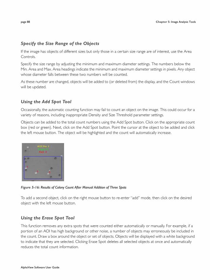
page 88 Chapter 5: Image Analysis Tools
Specify the Size Range of the Objects
If the image has objects of different sizes but only those in a certain size range are of interest, use the Area Controls.
Specify the size range by adjusting the minimum and maximum diameter settings. The numbers below the Min. Area and Max. Area headings indicate the minimum and maximum diameter settings in pixels. Any object whose diameter falls between these two numbers will be counted.
As these number are changed, objects will be added to (or deleted from) the display, and the Count windows will be updated.
Using the Add Spot Tool
Occasionally, the automatic counting function may fail to count an object on the image. This could occur for a variety of reasons, including inappropriate Density and Size Threshold parameter settings.
Objects can be added to the total count numbers using the Add Spot button. Click on the appropriate count box (red or green). Next, click on the Add Spot button. Point the cursor at the object to be added and click the left mouse button. The object will be highlighted and the count will automatically increase.
Figure 5-16: Results of Colony Count After Manual Addition of Three Spots
To add a second object, click on the right mouse button to re-enter “add” mode, then click on the desired object with the left mouse button.
Using the Erase Spot Tool
This function removes any extra spots that were counted either automatically or manually. For example, if a portion of an AOI has high background or other noise, a number of objects may erroneously be included in the count. Draw a box around the object or set of objects. Objects will be displayed with a white background to indicate that they are selected. Clicking Erase Spot deletes all selected objects at once and automatically reduces the total count information.
AlphaView Software User Guide

Colony Count page 89
Spot Count Data
When AlphaView opens, the Colony Count data box is hidden. To display spot count data, click the checkbox to deselect Hide Data. The following data window will appear:
Figure 5-17: Colony Count Data Window Showing AOI Summary Data
This window shows the summary data for the Area(s) of interest (AZ). This includes the threshold values that were set for each count type, the number of objects found for each count type, and the total pixels in all of the spots.
To see specific details on each spot, click View > Spot Details. Figure 5-18 displays an example of what displays:
Figure 5-18: Selecting the Colony Count Data Window to Show Individual Spot Details
The data table gives the individual spot number, the AOI in which it was counted, its coordinates, the pixel sum value for each spot, the area (number of pixels) for each spot, and the % contribution to the total.
AlphaView Software User Guide

page 90 Chapter 5: Image Analysis Tools
NOTE: Manually-added spots show areas of 1 pixel.
Multiplex Band AnalysisIn the ToolBox, Analysis Tools, a tab labeled Multiplex Band Analysis opens a set of tools with which the density of bands, spots or other objects can be measured. A two dimensional area of interest (or Object) is created and the density is obtained through the corresponding pixel intensity values.
Figure 5-19: Multiplex Band Analysis - Single and Multichannel Regional Tab
Creating an Object Area of Interest
Object Boxes:
An area of interest can be created in several ways. The user can manually draw an area of interest through the three OBJECT buttons. Objects can be enclosed with a box (rectangle), ellipse, or freehand drawing. Select the one that most closely corresponds to the shape of the objects on the image.
AlphaView Software User Guide
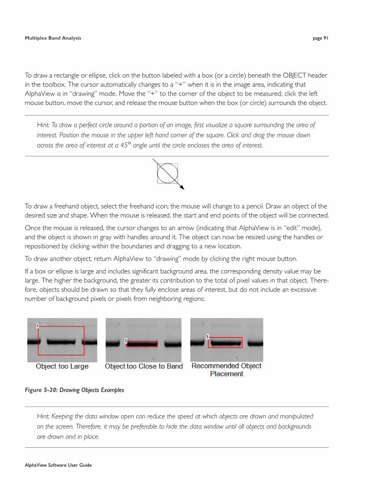
Multiplex Band Analysis page 91
To draw a rectangle or ellipse, click on the button labeled with a box (or a circle) beneath the OBJECT header in the toolbox. The cursor automatically changes to a “+” when it is in the image area, indicating that AlphaView is in “drawing” mode. Move the “+” to the corner of the object to be measured, click the left mouse button, move the cursor, and release the mouse button when the box (or circle) surrounds the object.
Hint: To draw a perfect circle around a portion of an image, first visualize a square surrounding the area of interest. Position the mouse in the upper left hand corner of the square. Click and drag the mouse down across the area of interest at a 45° angle until the circle encloses the area of interest.
To draw a freehand object, select the freehand icon; the mouse will change to a pencil. Draw an object of the desired size and shape. When the mouse is released, the start and end points of the object will be connected.
Once the mouse is released, the cursor changes to an arrow (indicating that AlphaView is in “edit” mode), and the object is shown in gray with handles around it. The object can now be resized using the handles or repositioned by clicking within the boundaries and dragging to a new location.
To draw another object, return AlphaView to “drawing” mode by clicking the right mouse button.
If a box or ellipse is large and includes significant background area, the corresponding density value may be large. The higher the background, the greater its contribution to the total of pixel values in that object. There-fore, objects should be drawn so that they fully enclose areas of interest, but do not include an excessive number of background pixels or pixels from neighboring regions:
Figure 5-20: Drawing Objects Examples
Hint: Keeping the data window open can reduce the speed at which objects are drawn and manipulated
on the screen. Therefore, it may be preferable to hide the data window until all objects and backgrounds are drawn and in place.
AlphaView Software User Guide

page 92 Chapter 5: Image Analysis Tools
Hint: Accurate Local Background Correction method requires the object box to contain a few pixel values that are true representations of the background level. If the object is too small and the band fills the object box then local background correction will result in significant errors.
Magic Wand and AutoSpot (Single Channel Only)
These two selections are automated detection features designed to recognize sample in an image and draw Object boxes around it. They are found under the Auto Detect heading in the main Multiplex Band Analysis tab. Once an object is created the dimensions can be altered and the background subtracted similar to manually drawn objects.
Figure 5-21: Magic Wand and AutoSpot Tools
Magic Wand
Selecting Magic Wand will activate a wand like symbol and the following data table:
Figure 5-22: Magic Wand Parameter Window
AlphaView Software User Guide

Multiplex Band Analysis page 93
The tip of the wand should be centrally positioned over the sample spot on the image and then simply click the mouse. The software will use either an “edge detection” algorithm to trace an area of interest around the spot or draw a box around the sample. A right mouse click will reactivate the wand icon for another selec-tion.
Magic Wand Sensitivity
The Magic Wand Sensitivity slide bar will alter the parameter for how much of the spot will be detected. The slide bar ranges from 0 to 100. The smaller the number the less of the spot the software will define. The greater the sensitivity number the more of the object the software will find.
HINT: Selecting a brighter pixel within the band (or spot) will have magic wand draw a tighter area of inter-est. Correspondingly, a less intense pixel will draw a larger perimeter around the selected spot.
Spot Type
Under the Spot Type heading the Bright Spots selection should be checked if the image contains bright spots on a dark background (e.g. ethidium bromide stained fluorescent gels and chemiluminescent blots). The Dark Spots selection should be made when the sample contains dark sample on a light background (example: film, Coomassie blue protein gels). The software should automatically determine this selection, but some manual intervention may be necessary. Remember as in all portions of AlphaView software if the image has been reversed (negative image) using the Reverse selection on the Contrast Adjustment window the Dark Spot selection should not be made. Reverse is a visual alteration only and does not affect the original image capture data. (e.g. a chemiluminescent blot is captured using the Reverse mode in order for it to appear as film, the correct selection is still Bright Spots).
Outline Type
Border Outline will use the edge detection methods to determine the spot area. Box Outline is the default setting and will draw a box shape around the sample usually including a significant portion of background. User preference and image particulars will determine which outline type is best.
AlphaView Software User Guide
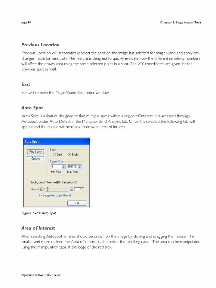
page 94 Chapter 5: Image Analysis Tools
Previous Location
Previous Location will automatically select the spot on the image last selected for magic wand and apply any changes made for sensitivity. This feature is designed to quickly evaluate how the different sensitivity numbers will affect the drawn area using the same selected point in a spot. The X,Y coordinates are given for the previous spot as well.
Exit
Exit will remove the Magic Wand Parameter window.
Auto Spot
Auto Spot is a feature designed to find multiple spots within a region of interest. It is accessed through AutoSpot under Auto Detect in the Multiplex Band Analysis tab. Once it is selected the following tab will appear and the cursor will be ready to draw an area of interest.
Figure 5-23: Auto Spot
Area of Interest
After selecting AutoSpot an area should be drawn on the image by clicking and dragging the mouse. The smaller and more defined the Area of Interest is, the better the resulting data. The area can be manipulated using the manipulation tabs at the edge of the red box.
AlphaView Software User Guide

Multiplex Band Analysis page 95
Options
The Options selection allows either a box outline to be drawn around the spots or a border outline. The box outline is the default setting and will include more of a background in the drawn area than the border outline. User preference and image particulars will determine which outline type is best for sensitivity can also be adjusted by sliding the bars for normal spots (<98% saturation) and for saturated spots (>98% saturation).
Figure 5-24: Auto Spot Options
Bright Spot vs Dark Spot
The Bright Spots selection should be checked if the image contains bright spots on a dark background (e.g. ethidium bromide stained fluorescent gels and chemiluminescent blots). The Dark Spots selection should be made when the sample contains dark sample on a light background (film, commassie blue protein gels etc.). The software should automatically determine this selection, but the user may have to override it if the software incorrectly evaluates an image. Remember as in all portions of AlphaView software if the image has been reversed (negative image) using the Reverse selection on the Contrast Adjustment window the Dark Spot selection should not be made. Reverse is a visual alteration only and does not effect the original image capture data. (EG if a chemiluminescent blot is captured using the Reverse mode in order for it to appear as film, the correct selection is still Bright Spots).
Find Spots
The Find Spot button is selected once the correct area of interest is drawn and the Bright Spot/Dark Spot selection is correctly made. A green outline will be drawn around the detected spots.
AlphaView Software User Guide
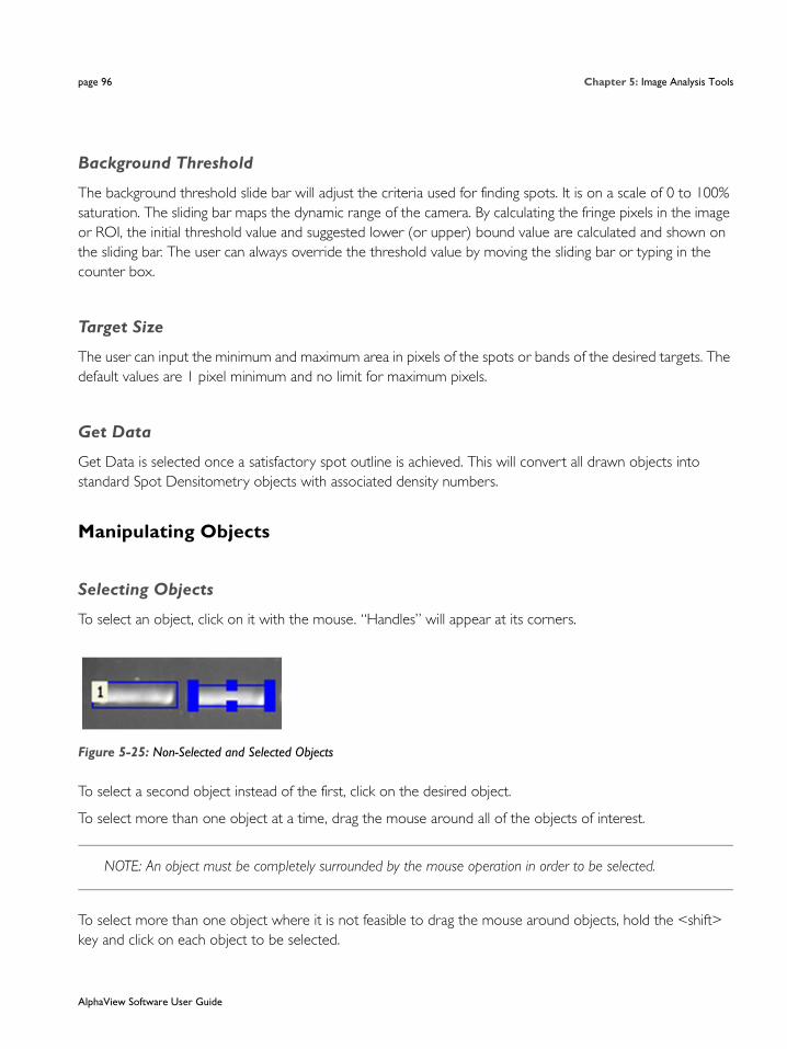
page 96 Chapter 5: Image Analysis Tools
Background Threshold
The background threshold slide bar will adjust the criteria used for finding spots. It is on a scale of 0 to 100% saturation. The sliding bar maps the dynamic range of the camera. By calculating the fringe pixels in the image or ROI, the initial threshold value and suggested lower (or upper) bound value are calculated and shown on the sliding bar. The user can always override the threshold value by moving the sliding bar or typing in the counter box.
Target Size
The user can input the minimum and maximum area in pixels of the spots or bands of the desired targets. The default values are 1 pixel minimum and no limit for maximum pixels.
Get Data
Get Data is selected once a satisfactory spot outline is achieved. This will convert all drawn objects into standard Spot Densitometry objects with associated density numbers.
Manipulating Objects
Selecting Objects
To select an object, click on it with the mouse. “Handles” will appear at its corners.
Figure 5-25: Non-Selected and Selected Objects
To select a second object instead of the first, click on the desired object.
To select more than one object at a time, drag the mouse around all of the objects of interest.
NOTE: An object must be completely surrounded by the mouse operation in order to be selected.
To select more than one object where it is not feasible to drag the mouse around objects, hold the <shift> key and click on each object to be selected.
AlphaView Software User Guide
Multiplex Band Analysis page 97
To de-select an object, click the left mouse button outside of the selected object. The handles disappear, indicating that the object is no longer selected.
Copying Objects
To draw boxes or ellipses enclosing the same number of data points, use the Copy function.
First, draw or select an object of the desired shape and size as described above. Next, click on the Copy but-ton in the toolbox. A duplicate of the selected object will appear on the screen. This object can then be moved to the desired position.
To make multiple copies of an object, continue to click on the Copy button until the desired number of copies is displayed.
Moving Objects
An object can be moved to fine-tune its position simply by clicking on it, holding down the left mouse button and dragging it to the desired location.
Deleting Objects
To remove an object or set of objects, select the object(s). Select the Delete button on keyboard. All the selected objects are removed from the image window and their associated data is cleared from the data window.
Multiplex Band Analysis Measurements
As objects are drawn, their density data is automatically calculated and displayed in a data window. Any time an object is drawn or detected, the data in the window are updated. If the Multiplex Band Analysis Results window obscures a region of interest, resize and/or move it following Windows conventions.
AlphaView Software User Guide
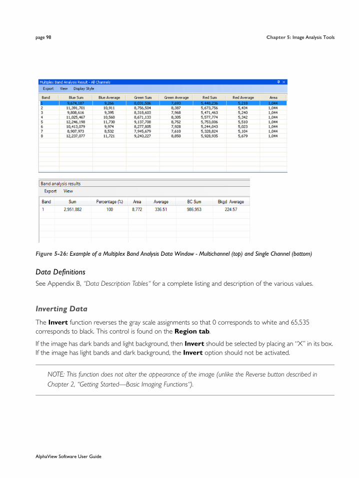
page 98 Chapter 5: Image Analysis Tools
Figure 5-26: Example of a Multiplex Band Analysis Data Window - Multichannel (top) and Single Channel (bottom)
Data DefinitionsSee Appendix B, “Data Description Tables“ for a complete listing and description of the various values.
Inverting Data
The Invert function reverses the gray scale assignments so that 0 corresponds to white and 65,535 corresponds to black. This control is found on the Region tab.
If the image has dark bands and light background, then Invert should be selected by placing an “X” in its box. If the image has light bands and dark background, the Invert option should not be activated.
NOTE: This function does not alter the appearance of the image (unlike the Reverse button described in Chapter 2, “Getting Started—Basic Imaging Functions“).
AlphaView Software User Guide

Multiplex Band Analysis page 99
Background Tab–Calculating Background Values
Figure 5-27: Background Tab
Background subtraction is an important part of image densitometry analysis. The Background tab is used to subtract the background in the image from the regions of interest. The background is unwanted signal in the region arising from the fluorescence detection chemistry, the membrane and quality of the sample itself. Because fluorescence detection is extremely sensitive, high background levels in the image can be a common problem, especially in the early stages of protocol development. Fluorescence protocols require careful attention to cleanliness and sample handling to minimize background problems.
Regional Background Background region applied to all object regions. Place a background region in an area of the image representative of the background level for all channels. The image contrast display should be adjusted to so that the variations in the background can be seen so that the background region(s) may be placed in an area best representative of the background.
NOTE: More than one background region can be used and the average pixel level of all the background regions is applied. The data table is automatically updated with Background Corrected (BC) values.
AlphaView Software User Guide

page 100 Chapter 5: Image Analysis Tools
Multi-Regional Background Background region applied to a subset of object regions. A second (or third) background region can then be applied to a second (or third) subset of object regions. Each subset of object regions is corrected by the linked background region to account for differences in background level across an image.
Local Background Background region applied using the average of the 10 lowest pixels in a band region. The regions should be slightly larger than the bands to use properly apply this method of background correction. The data table is automatically updated with the Background corrected intensity values.
None (No Background)If no background calculation method has been selected, the background value in the data window (BACK) is reported as zero (0). Recommendation: No Background or Manual Background is suggested for AutoSpot, Magic Wand (only the border outlines though) or any object where little if any background is included in the object area of interest.
Background Link/Unlink Tool
Link Background Applied in conjunction with Multi-Regional Background to link a background region to a subset of object regions. First place a background region in an area of the image representative of the background specific to the subset of object regions. Draw a rectangle by left clicking on the image and dragging to include the desired subset of bands and a single background region to be linked. Alternatively use Ctrl left click to select multiple regions and the specific background region. Then select the Link Background button. The data table is updated with Background corrected values.
Unlink Background Tool Used to unlink the background regions from the band subsets.
Figure 5-28: Unlink Background Tool
B1 (background) and data box 2 (region) are selected and Linked as shown.
When using the region and multiregional background correction methods there are two points to consider. First, note that a background region applied to a multichannel image extracts and applies the background values on each channel using the respective background and region values for that channel. For a three chan-
AlphaView Software User Guide

Multiplex Band Analysis page 101
nel image, for example, Blue, Green and Red background values are extracted and applied to the Blue, Green Red channel object regions respectively. Second, note that the background correction is automatically adjusted for any differences in area between the background and object regions as f006Fllows.
Data Definitions
For regions with different area the relevant quantities are adjusted for the relative region area to obtain accurate corrected values. For example if local background correction is used the “area” is 10 pixels for the background region. When this value is used to correct a data region the actual value used is scaled such that the 10 pixel area appears to be the same area as the data region. In this way regions with different areas are accurately accounted for in all calculations.
Figure 5-29: Multichannel Image with Regional Background
A multichannel image with regional background applied. The background values from a single region are extracted and applied to each of the three channels respectively.
Background Corrected (BC) Average: Background Corrected Average = (Region Average–Bkgd Region Average)
Background Corrected (BC) Sum: Background Corrected Sum = (BC region Average*Region Area)
AlphaView Software User Guide

page 102 Chapter 5: Image Analysis Tools
Figure 5-30: Band Correct Values
The data table showing the respective Background Corrected (BC) Average values for each channel after regional background correction.
NOTE: The Signal/Noise ratio is greater than 3 (indicating a significant signal level) for regions 17 to 24 in the Blue channel, regions 2-8 and regions 17-24 in the Green channel and for regions 9 to 16 in the Red channel corresponding to the visible bands in the image. Be aware that the actual biological variation (best seen by observing the signals from replicate samples) will be much greater than the signal/noise ratios from the image data.
Control Tab
The Control tab is used to apply loading controls and a positive control to the data.
NOTE: While the background regions are not displayed in the control tab the background corrected data values are maintained in the Data Table and are used in the calculations.
AlphaView Software User Guide
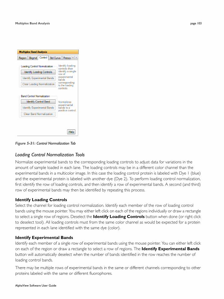
Multiplex Band Analysis page 103
Figure 5-31: Control Normalization Tab
Loading Control Normalization ToolsNormalize experimental bands to the corresponding loading controls to adjust data for variations in the amount of sample loaded in each lane. The loading controls may be in a different color channel than the experimental bands in a multicolor image. In this case the loading control protein is labeled with Dye 1 (blue) and the experimental protein is labeled with another dye (Dye 2). To perform loading control normalization, first identify the row of loading controls, and then identify a row of experimental bands. A second (and third) row of experimental bands may then be identified by repeating this process.
Identify Loading Controls Select the channel for loading control normalization. Identify each member of the row of loading control bands using the mouse pointer. You may either left click on each of the regions individually or draw a rectangle to select a single row of regions. Deselect the Identify Loading Controls button when done (or right click to deselect tool). All loading controls must from the same color channel as would be expected for a protein represented in each lane identified with the same dye (color).
Identify Experimental Bands Identify each member of a single row of experimental bands using the mouse pointer. You can either left click on each of the region or draw a rectangle to select a row of regions. The Identify Experimental Bands button will automatically deselect when the number of bands identified in the row reaches the number of loading control bands.
There may be multiple rows of experimental bands in the same or different channels corresponding to other proteins labeled with the same or different fluorophores.
AlphaView Software User Guide
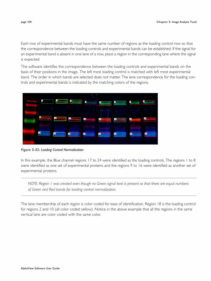
page 104 Chapter 5: Image Analysis Tools
Each row of experimental bands must have the same number of regions as the loading control row so that the correspondence between the loading controls and experimental bands can be established. If the signal for an experimental band is absent in one lane of a row, place a region in the corresponding lane where the signal is expected.
The software identifies the correspondence between the loading controls and experimental bands on the basis of their positions in the image. The left most loading control is matched with left most experimental band. The order in which bands are selected does not matter. The lane correspondence for the loading con-trols and experimental bands is indicated by the matching colors of the regions.
Figure 5-32: Loading Control Normalization
In this example, the Blue channel regions 17 to 24 were identified as the loading controls. The regions 1 to 8 were identified as one set of experimental proteins and the regions 9 to 16 were identified as another set of experimental proteins.
NOTE: Region 1 was created even though no Green signal level is present so that there are equal numbers of Green and Red bands for loading control normalization.
The lane membership of each region is color coded for ease of identification. Region 18 is the loading control for regions 2 and 10 (all color coded yellow). Notice in the above example that all the regions in the same vertical lane are color coded with the same color.
AlphaView Software User Guide
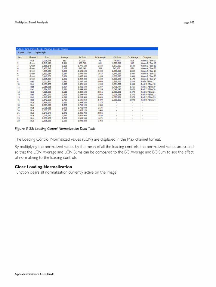
Multiplex Band Analysis page 105
Figure 5-33: Loading Control Normalization Data Table
The Loading Control Normalized values (LCN) are displayed in the Max channel format.
By multiplying the normalized values by the mean of all the loading controls, the normalized values are scaled so that the LCN Average and LCN Sums can be compared to the BC Average and BC Sum to see the effect of normalizing to the loading controls.
Clear Loading NormalizationFunction clears all normalization currently active on the image.
AlphaView Software User Guide

page 106 Chapter 5: Image Analysis Tools
Data Definitions
Band Control Normalization Normalize regions of experimental bands to a reference band control. First select the channel and identify the region for the positive control and then identify the regions for the experimental bands. The control band and the corresponding experimental bands must be in the same channel. Multiple groups of positive controls and experimental bands may be identified and each set may be in a distinct channel.
Identify Control Band Identify the control band using the mouse pointer. Select the Identify Experimental Bands tool to identify the experimental bands to be normalized to this control band. Bands can be selected
You can either left click on each of the regions or draw a rectangle to select a row of regions. Deselect the Identify Experimental Bands or right click when done.
Figure 5-34: Band Control Normalization
In this example, region 2 in the Green channel was selected as a control band and regions 3 to 8 were selected as the associated experimental bands. Then region 9 was selected as a control band in the Red channel and regions 10-16 were selected as the associated experimental bands.
LCN Sum Loading Control Normalized Sum = (LCN Average* Area)
LCN Average Loading Control Normalized Average = (BC Average of Experimental Band/BC Average of corresponding Loading control) * mean of all loading controls
LC Regions Specifies the channel and region number used for each Experimental Band and corresponding Loading Control, (e.g. Red1/ Green 12)
AlphaView Software User Guide

Multiplex Band Analysis page 107
NOTE: Regions outlines are dashed to indicate the corresponding control and experimental bands.
After identifying the control and experimental bands the Data table is updated with four additional columns, PCN Sum, PCN Average, PC Regions and Fold Change (PCN Positive Control Normalized). The control band is assigned a PCN Average value of 100 and the normalized experimental bands are adjusted to this value in PCN average column.
Figure 5-35: Band Control Normalization Data Table
In this example, region 2 in the Green channel corresponds to a negative control band and Region 9 in the Red channel corresponds to a negative control band. The PCN average values for regions 3 to 8 show the sig-nal level relative to the control band and regions 10 to 16 show the signal level relative to the control band.
If a loading control has been applied to all selected bands then the loading control normalized LCN average values are used in the PCN calculation. If loading control normalization has not been done then the BC values are used and if no background correction has been applied then the Average values are used.
Data Definitions
PCN Sum Positive Control Normalized Sum= (PCN Average *Area)
PCN Average Positive Control Normalized Average = (LCN Average of experimental band / LCN Average of control band) *100
AlphaView Software User Guide
page 108 Chapter 5: Image Analysis Tools
NOTE: In the Data table there are columns available for Blue/Green, Blue/Red, etc. These columns display the ratio of the indicated channel Sums (or BC Sums) for that region and are intended for analysis of dual labeled bands or spots as may encountered in dot blots. These ratios are somewhat arbitrary as they depend on the relative exposure times of the channels. Do not confuse these ratios with the LC regions or BC regions which indicate which regions are selected as control and experimental bands respectively.
See Appendix D, “Fully Worked Examples of Multicolor Band Analysis“ for a detailed example of analysis of a phosphorylation study using multicolor western methods using loading controls and Band controls.
Mass Standard Calibration Curves for Quantitative PCR
The button in the Multiplex Band Analysis toolbox labeled Std Curve opens a set of tools that create a calibration curve for applications such as quantitative PCR and Western Blot band quantization. The calibration curve functions allow quantization of the bands on a gel based on a set of standards. A minimum of two standard bands must be input, but the accuracy of the calibration curve increases as the number of stan-dard bands and their range of values increase.
Defining the Bands as Objects
Before generating a standard curve, define the bands using the object drawing tools in the Multiplex Band Analysis toolbox. As described in “Selecting Objects” on page 96, the size of an object can influence the pixel sum value. Therefore, we recommend using the same sized box, ellipse or freehand drawing when defining a standard curve. (For instructions, see “Copying Objects” on page 97.)
Specifying the Quantization Units
Once the objects are defined, click on the Std Curve tab. The Standard Curve Toolbox will appear in which the results should be reported (e.g. ng, μL, pg, %) in the Enter units box
PC Regions Specifies the channel and region number used for each Experimental Band and corre-sponding Band Control, (e.g. Red1/ Red 6)
Fold Change Fold Change of experimental band relative to control. If LCN Average experimental band > LCN Average control band then fold change = LCN average experimental / LCN average control. If LCN Average of the experimental band < LCN Average of control, then fold change = (-1) * 1/ (LCN average experimental / LCN average.
AlphaView Software User Guide

Multiplex Band Analysis page 109
Figure 5-36: Standard Curve Tab
Designating the Standard Bands
Select Add Items and select the color channel (in Figure 5-36, the Red channel has been selected) and select the appropriate regions created using the object drawing tool. Continue to select regions until all regions used for standard curve calculation are listed. For each band whose value (in Figure 5-36, the Red background cor-rected average is selected) is known enter the concentration in the last column as shown in Figure 5-37.
Figure 5-37: Standard Curve Input for Known Concentration (expressed in nanograms)
In the Band/Sum/concentration box displayed, enter the value for the band. When the value is inserted, click on the OK button. The band number changes from white to green, indicating that it is now a standard (see Figure 5-38).
AlphaView Software User Guide

page 110 Chapter 5: Image Analysis Tools
Figure 5-38: The Standard Curve spreadsheet
Once a second value has been entered, a curve is displayed. The points corresponding to the standard bands are labeled in green. Points for the unknown objects on the image are displayed on the standard curve based on their selected values. These are labeled in white. Enter values for each band whose amount is known. As more standard points are added, the calculated values of the unknown points may change. The relevant values for the best fit curve and the corresponding equation, along with the coefficient of correlation, is displayed.
Figure 5-39: Standard Curve - Green spots are the entered standard values, yellow spots are quantified unknown values.
NOTE: Cubic spline and point-to-point curves have no equation nor r2 value. These values are displayed only for linear regression and log linear regression fit models.
To remove a band from the set of standards, click on it again. The band number changes from green back to white, indicating that it is no longer a standard. To de-select all the standard points at once, click on the Remove Items button in the toolbox.
To change the value of a standard band, click on it once in the spreadsheet. Insert the new value and select Enter on the keyboard to input the value. The value will be updated in the graph with a new value calculated for any unknown band if appropriate.
AlphaView Software User Guide

Multiplex Band Analysis page 111
Displaying the Curve
If the box displaying the standard curve obscures a part of the image, it can be resized using Windows oper-ating system functions. It can be hidden from view by clicking the Graph checkbox in the Standard Curve tool-box.
Quantization Values of Unknown Bands
As the values for the standard bands have been entered, the quantization values of the unknown bands are automatically calculated. The calculated values of the unknowns are automatically updated in the spreadsheet. It is possible that the graph display may need to be refreshed after changes in standards values, adding/deleting regions, etc. To refresh the graph display simply uncheck and recheck the graph control checkbox on the Std Curve tab.
NOTE: The graph is based on a several different graph equations (shown in the Toolbar).
Figure 5-40: Multiplex Band Analysis Data Box
The third column in the data box contains values for the standards (entered by the user) highlighted in green, and the values for the unknown bands (calculated based on the curve). The heading of this column reflects the units entered as in Specifying the Quantization Units above.
Standards have an “s” next to the object number, and are highlighted in green to differentiate them from unknown bands.
Values that are outside the range defined by the standards are not quantified and simply have a dash entered in the corresponding column.
Quantization Values of Unknown Bands across Color Channels
A specially constructed control sample (Color Channel Normalization Control – or CCN) is required to make quantitative comparisons between different color channels in a multicolor image. One such sample is a mixture of a single type of protein or appropriate size (similar in size to the other proteins of interest) that has three different fluorescent labels. The GE DIGE minimal dye labeling kit can be used to label aliquots of the
AlphaView Software User Guide
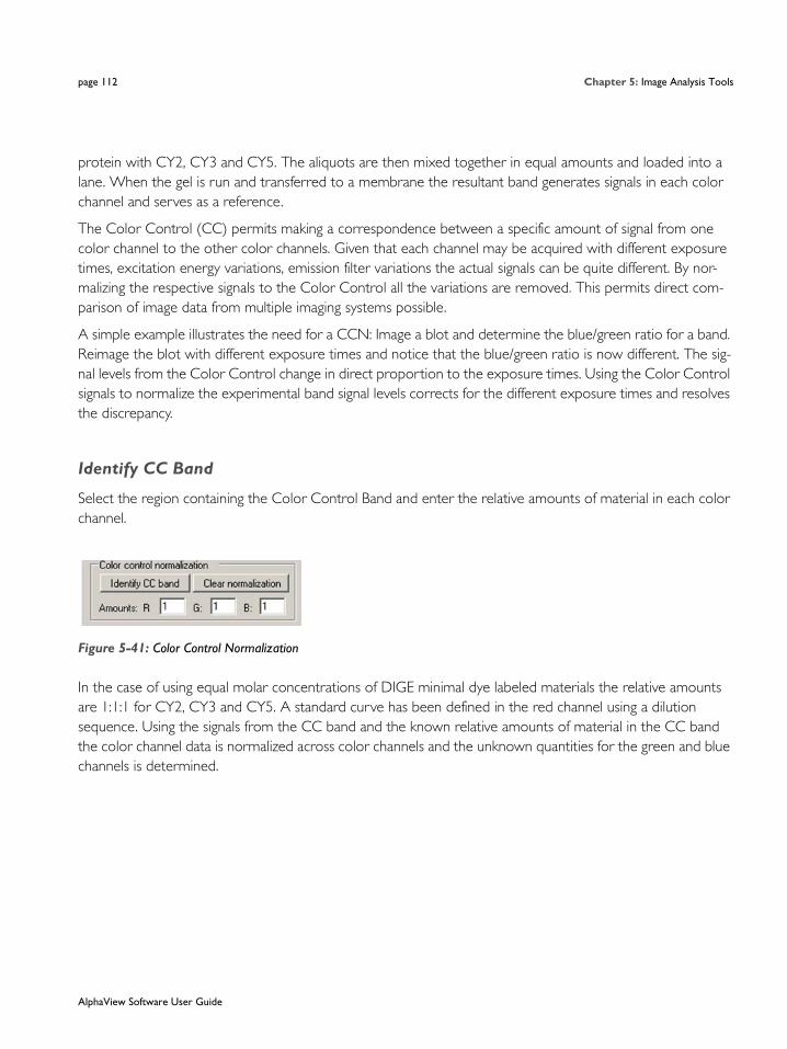
page 112 Chapter 5: Image Analysis Tools
protein with CY2, CY3 and CY5. The aliquots are then mixed together in equal amounts and loaded into a lane. When the gel is run and transferred to a membrane the resultant band generates signals in each color channel and serves as a reference.
The Color Control (CC) permits making a correspondence between a specific amount of signal from one color channel to the other color channels. Given that each channel may be acquired with different exposure times, excitation energy variations, emission filter variations the actual signals can be quite different. By nor-malizing the respective signals to the Color Control all the variations are removed. This permits direct com-parison of image data from multiple imaging systems possible.
A simple example illustrates the need for a CCN: Image a blot and determine the blue/green ratio for a band. Reimage the blot with different exposure times and notice that the blue/green ratio is now different. The sig-nal levels from the Color Control change in direct proportion to the exposure times. Using the Color Control signals to normalize the experimental band signal levels corrects for the different exposure times and resolves the discrepancy.
Identify CC Band
Select the region containing the Color Control Band and enter the relative amounts of material in each color channel.
Figure 5-41: Color Control Normalization
In the case of using equal molar concentrations of DIGE minimal dye labeled materials the relative amounts are 1:1:1 for CY2, CY3 and CY5. A standard curve has been defined in the red channel using a dilution sequence. Using the signals from the CC band and the known relative amounts of material in the CC band the color channel data is normalized across color channels and the unknown quantities for the green and blue channels is determined.
AlphaView Software User Guide

Multiplex Band Analysis page 113
Figure 5-42: Band Analysis Results - All Channels
In Figure 5-42, band 4 now shows ng quantities for each color channel. These quantities are also shown on the standard curve graph.
Figure 5-43: Standard Curve
See Appendix D, “Fully Worked Examples of Multicolor Band Analysis“ for a detailed analysis shown use of CCN to determine the amount of phosphorylated versus non-phosphorylated protein isoforms.
AlphaView Software User Guide

page 114 Chapter 5: Image Analysis Tools
Lane ProfileThe Lane Profile option in the Analysis Tools tab of the ToolBox accesses a set of densitometry and molecular weight determination tools with which bands on a gel can be automatically analyzed in a lane for-mat.
When Lane Profile is selected, the Lanes tab is displayed with the following functions:
Figure 5-44: Lane Profile Lanes Tab
Profile Path Width
The Profile Path Width is the area from which the pixel density is measured. The default setting is 10. To adjust the setting, click on the up or down arrows or enter a value and hit the enter button on the keyboard.
The density values for Lane Profile graphs are determined by the average pixel density between the blue lines on the template.
A Profile Path Width that is too narrow may not include enough information and can result in a noisy graph. By contrast, a Profile Path Width that is too wide can incorporate background pixels that will reduce the pixel average and dilute the actual data.
AlphaView Software User Guide
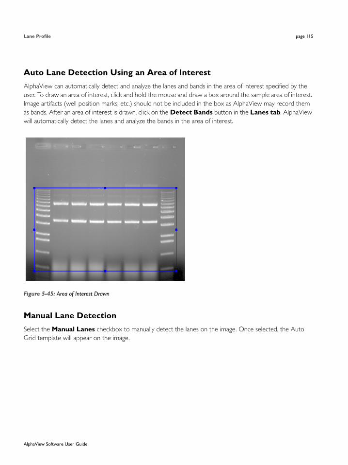
Lane Profile page 115
Auto Lane Detection Using an Area of Interest
AlphaView can automatically detect and analyze the lanes and bands in the area of interest specified by the user. To draw an area of interest, click and hold the mouse and draw a box around the sample area of interest. Image artifacts (well position marks, etc.) should not be included in the box as AlphaView may record them as bands. After an area of interest is drawn, click on the Detect Bands button in the Lanes tab. AlphaView will automatically detect the lanes and analyze the bands in the area of interest.
Figure 5-45: Area of Interest Drawn
Manual Lane Detection
Select the Manual Lanes checkbox to manually detect the lanes on the image. Once selected, the Auto Grid template will appear on the image.
AlphaView Software User Guide

page 116 Chapter 5: Image Analysis Tools
Figure 5-46: Lane Profile Auto Grid Template
Setting Up the Lane Profile Template
Red lines in the Auto Grid template indicate borders of adjacent lanes. Green lines define the Profile Path Width.
Manual Lanes BoxSelect the Number of Lanes up to a maximum of 24 lanes. When the number of lanes is adjusted, the template displayed on the image is updated accordingly.
If the lanes on the gel are horizontally oriented (sideways) the image can be rotated. To change the orienta-tion of the image to coincide with the template, click on the Enhancement Tools tab in the Toolbox and select the Rotate-Flip option. Click and drag the rotation bar +/- 90 degrees until the desired orientation is reached.
After specifying the correct number of lanes and changing the image orientation, adjust the outside borders of the template until they frame the lanes to be scanned. To do this, first click on the template. Next, select any of the blue boxes along the outside border of the template and drag it until the desired size is reached. Adjust the template until the border of the template frames the lanes to be scanned and the red lines lie between each of the lanes.
If the lanes of the gel are not perfectly straight, click the Skewing checkbox in the Manual Lanes box. The template will display four blue boxes, one at each corner of the template. Click and drag the blue boxes as needed until the template is positioned properly over the skewed lanes.
AlphaView Software User Guide

Lane Profile page 117
Figure 5-47: Skewed Lane Profile Template Properly Aligned on a Gel
Profile Path WidthAdjust the Profile Path Width value as needed. The path width should not exceed the band edges and cannot extend beyond the red lane borders. As this value is changed, the template displayed on the image updates accordingly.
Bands Darker than Background Option
Select the Bands darker than background checkbox if the image being analyzed has dark bands/signal on a white background which are usually colorimetric gels. The Bands darker than background option is only necessary when the actual sample has signals that are visible by the naked eye, for example Coomassie Blue stained gels, Silver stained gels, and pieces of autorad film.
Image Analysis–Detect Bands
Select the Detect Bands button to automatically measure and calculate the densities of each lane. To have AlphaView detect all bands in the image automatically select Detect Bands immediately after opening an image. Otherwise, select Detect Bands after drawing an area of interest or after the Manual Lane settings and template have been adjusted.
Viewing Results
Once the Detect Bands button is selected, AlphaView automatically analyzes the image, detects the peaks for each lane, integrates the area under each peak, displays results and moves to the Bands tab.
AlphaView Software User Guide

page 118 Chapter 5: Image Analysis Tools
Figure 5-48: Lane Profile Bands Tab
Peak integration adjustments that can be made manually will be described in detail later in this section. The Analyzed Image and the Lane Profile Results windows are displayed.
Analyzed Image
Individual bands will be identified by number on the analyzed image. When a lane is selected in the image its borders will turn pink. The corresponding lane data will be displayed in the Lane Profile Results windows.
AlphaView Software User Guide

Lane Profile page 119
Figure 5-49: Analyzed Image
Lane Profile Results Windows
The following results windows will also be displayed after the image is analyzed. These windows can be resized or docked by the user if desired:
• Data Table (middle). The Data Table displays peak information for each lane in the image.
• Lane Graphs (lower left). This area displays a graph for each lane.
• Active Graph (lower right). The active graph displays peak numbers and integration data for the lane selected.
To view data and the Active Graph for a lane, select a lane either from Analyzed Image or from the Lane Graphs. To view peak data for a specific band, select the band in the Analyzed Image or the peak from the Active Graph. The corresponding data will be highlighted in the Data Table. AlphaView uses the following color-coding to indicate what data is being displayed:
• The lane graph that is currently selected will be grey.
• The data for the currently selected lane will be highlighted in yellow in the Data Table.
• The data for the currently selected band or peak will be highlighted in dark yellow in the Data Table, and the peak fill in the Active Graph will also be dark yellow.
AlphaView Software User Guide

page 120 Chapter 5: Image Analysis Tools
Figure 5-50: Results showing Color Coding in Data Table (top), Lane Graph (lower left) and Active Graph (lower right)
Lane Graph DisplayGraphs representing all Analyzed Image lanes are shown in this area. After band detection, Lane 1 will be selected by default and its corresponding peak data will also be displayed in the Data Table and Active Graph. To view data for a different lane simply click on its lane graph.
When the image contains many lanes, there may be too many graphs in the Lane Graph display to see rea-sonable detail. To reduce this view to only four lane graphs, select the Options menu directly above the Data Table and deselect Show All Lanes.
Figure 5-51: Deselecting Show All Lanes
AlphaView Software User Guide

Lane Profile page 121
Active GraphThe Active Graph is shown in the lower right. The x-axis represents the distance (in pixels) from the top of the area of interest drawn or the Auto Grid template used. The y-axis represents the average pixel intensity across the width of the scan.
NOTE: Active Graphs are shown without axes in order to show as much detail as possible in a small win-dow. To show the graph’s axes, choose Show Axes from the Show Single Lanes option in the Options menu located above the Data Table.
Data TableOnce a peak is defined, its integration data and associated information are displayed in the Data Table. The data table is updated automatically when peaks are added or deleted, when peak boundaries are redefined, or if the background value is reset.
Figure 5-52: Example Data Table
The Data Table contains the following columns of data:
• LANE indicates the lane number where the peak is located.
• PEAK is the number assigned to each peak on the graph.
• DISTANCE is the migration distance (in pixels) for each peak as measured from the top of the region used for data analysis.
• WIDTH and HEIGHT are the calculated peak width and peak height.
• AREA is the integrated pixel intensity for the area under each peak and can be used to represent band intensity.
AlphaView Software User Guide
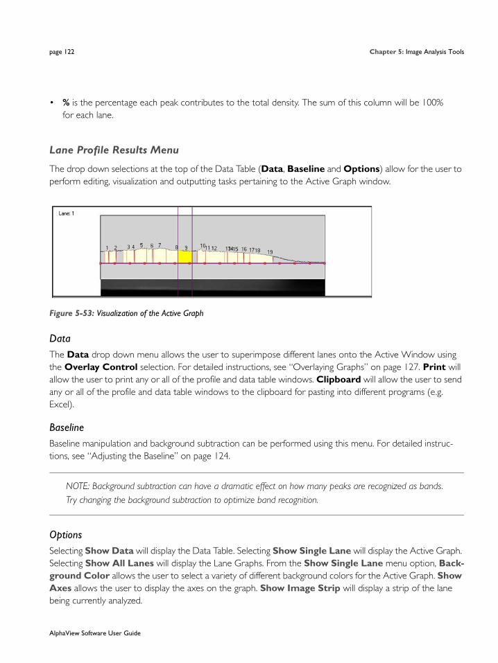
page 122 Chapter 5: Image Analysis Tools
• % is the percentage each peak contributes to the total density. The sum of this column will be 100% for each lane.
Lane Profile Results Menu
The drop down selections at the top of the Data Table (Data, Baseline and Options) allow for the user to perform editing, visualization and outputting tasks pertaining to the Active Graph window.
Figure 5-53: Visualization of the Active Graph
DataThe Data drop down menu allows the user to superimpose different lanes onto the Active Window using the Overlay Control selection. For detailed instructions, see “Overlaying Graphs” on page 127. Print will allow the user to print any or all of the profile and data table windows. Clipboard will allow the user to send any or all of the profile and data table windows to the clipboard for pasting into different programs (e.g. Excel).
BaselineBaseline manipulation and background subtraction can be performed using this menu. For detailed instruc-tions, see “Adjusting the Baseline” on page 124.
NOTE: Background subtraction can have a dramatic effect on how many peaks are recognized as bands. Try changing the background subtraction to optimize band recognition.
OptionsSelecting Show Data will display the Data Table. Selecting Show Single Lane will display the Active Graph. Selecting Show All Lanes will display the Lane Graphs. From the Show Single Lane menu option, Back-ground Color allows the user to select a variety of different background colors for the Active Graph. Show Axes allows the user to display the axes on the graph. Show Image Strip will display a strip of the lane being currently analyzed.
AlphaView Software User Guide

Lane Profile page 123
Figure 5-54: Options > Show Single Lane Menu
Editing Peaks
Editing Peak BoundariesThe boundaries of existing peaks can be readjusted to make the peaks wider or narrower. To adjust either peak boundary, click on the peak to select it. Next, point the cursor at the vertical boundary line, hold down the left mouse button and drag the line to the desired location. When it is in place, release the mouse button.
The data table is automatically updated to reflect any adjustments. Both the peak and the data in the data table will be blue to indicate that this is a user-defined (vs. automatically detected) peak.
Visualizing Peak PlacementsTo determine exactly where a peak is located relative to the original image, it is often helpful to see the graph and the gel image in the same orientation. The Show Strip function (found in the Options menu) displays the area of the gel that has been defined as a lane across the length of the x-axis.
Figure 5-55: Graph With Show Strip Selected
NOTE: If Show Strip fails to show a portion of the image, check that the appropriate driver for the VGA card is selected.
AlphaView Software User Guide
page 124 Chapter 5: Image Analysis Tools
Adjusting the Baseline
As a default, the baseline value is set to Auto Base. As the baseline is adjusted, the values for all peaks are updated to reflect the new baseline.
All of the following functions are found in the Baseline menu under Background Subtraction:
Auto BaseThis method breaks the red line defining the left boundary of the lane into sixteen regions, and outputs sixteen points which reflect the average backgrounds across those sixteen regions. The user can manipulate the 16 points by clicking and dragging. The user may also designate more points than the 16 and manipulate those in the same fashion.
Intra-LaneThis method uses the lower of the two values at the edges of the lane along its travel as the background. If the section of the image is used is wider than the bands, then this is a very effective way of removing co-migrating material from your measurements. This method should only be used if the bands are completely enclosed. This is because when the edges of your lane area intersect any of your bands, band material will be consid-ered as background, severely affecting your results.
Rubber BandThis method can be thought of as stretching a rubber band underneath the lane profile. This option does not work well if the values at the ends of the intensity profile are lower than the rest of the intensity pixels. We do not recommend this method for images with poorly separated bands.
Minimum ProfileThis method takes the lowest value on the profile of each lane as the background for that lane. We do not recommend this method for lanes where the beginning or end of the lane is the lowest point as this is dependent on where the lane boundary was placed when it was defined. This can be hard to repeat between analysis of the same gel.
Valley to ValleyThis method requires that you have performed band detection first. The background is taken as the line between the edges of the bands in the lane. You enter a value (see “Set Parameters” on page 125) of maximum slope in the accompanying entry box to avoid situations where the edge between overlapping bands, which is not at the background intensity, causes the background to climb too high.
AlphaView Software User Guide
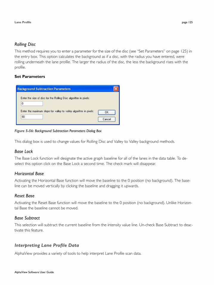
Lane Profile page 125
Rolling DiscThis method requires you to enter a parameter for the size of the disc (see “Set Parameters” on page 125) in the entry box. This option calculates the background as if a disc, with the radius you have entered, were rolling underneath the lane profile. The larger the radius of the disc, the less the background rises with the profile.
Set Parameters
Figure 5-56: Background Subtraction Parameters Dialog Box
This dialog box is used to change values for Rolling Disc and Valley to Valley background methods.
Base LockThe Base Lock function will designate the active graph baseline for all of the lanes in the data table. To de-select this option click on the Base Lock a second time. The check mark will disappear.
Horizontal BaseActivating the Horizontal Base function will move the baseline to the 0 position (no background). The base-line can be moved vertically by clicking the baseline and dragging it upwards.
Reset BaseActivating the Reset Base function will move the baseline to the 0 position (no background). Unlike Horizon-tal Base the baseline cannot be moved.
Base SubtractThis selection will subtract the current baseline from the intensity value line. Un-check Base Subtract to deac-tivate this feature.
Interpreting Lane Profile Data
AlphaView provides a variety of tools to help interpret Lane Profile scan data.
AlphaView Software User Guide

page 126 Chapter 5: Image Analysis Tools
V. LineTypically, the peaks on a graph correspond to the bands in a lane. The V. Line tool located in the Lane Graph Display can help determine if the peaks on two different graphs represent bands at the same molecular weight position (i.e. the same distance from the top of the gel).
To compare peaks on different graphs, roll the mouse over the Lane Graphs. A vertical line which can be scrolled across the graphs will appear. The intensity value at the point where the V. Line crosses the graph will be displayed.
Figure 5-57: V.Line Tool Intensity Display
Alternatively, the V. Line can also display hash marks which is a useful tool for comparing peak heights. To toggle between displaying intensity values and hash marks when using the V. Line, click the right mouse but-ton.
Figure 5-58: V.Line Tool Hash Marks Display
NOTE: The hash marks are most useful when only four graphs are shown so that enough detail is dis-played. To change the Lane Graph display, select the Options menu which is directly above the Data Table and deselect Show All Lanes.
AlphaView Software User Guide

Lane Profile page 127
Overlaying GraphsWhen comparing the bands in one lane with those in another it is often convenient to display the graphs so that one is superimposed over another. After clicking on a graph so that it is enlarged in the image area, select the Overlay Control function (from the Data menu) to display the Lane Overlay Control dialog box. In this dialog box, specify the lane(s) whose graph(s) should be superimposed and the color and line pattern in which they should be displayed.
• The first column in the dialog box contains the numbers of the graphs which can be superimposed.
• The second column reports whether or not the graph of a particular lane is currently superimposed. These ON/OFF settings toggle back and forth by clicking on them.
• The colored bar in the third column indicates the color in which a graph will be displayed when it is superimposed. To select a color option, click on the color bar until the desired color is shown.
• The last column in the dialog box specifies the pattern of the line when the graph is superimposed. To select a pattern, click on the current pattern until the desired pattern is shown.
It is especially important to choose different patterns if the graphs will be printed, as differ-ent colors cannot be distinguished using a gray scale printer.
When the selections have been made, click on the DONE button to dismiss the dialog box and superimpose the selected graph(s). (If no graphs have been selected, the dialog box is simply dismissed.)
Figure 5-59: Three Graphs Overlaid
To turn all graph superimposing off, select the Deselect All button at the bottom of the dialog box.
Bands Tab Overview
Several lane editing and viewing options appear in the Bands tab. Each will be explained in detail in this sec-tion.
AlphaView Software User Guide

page 128 Chapter 5: Image Analysis Tools
Figure 5-60: Lane Editing Features
Add LaneThis option allows an additional lane to be placed on the image. To add a lane, select the Add Lane button and place the mouse on the image. A plus sign cursor with a new lane grid will display on the image where lanes can be added. Roll the mouse over the image to move the cursor to the desired position. When the desired position is reached, click the mouse to drop the lane on the image. To add more lanes, move the cur-sor to another position on the image and click to add the next new lane. Continue until all new lanes are added. Click the Add Lane button again to exit the editing mode. The Data Table will readjust accordingly, adding the lane and calculating results for the bands within the lane.
Delete LaneThis option allows lanes to be deleted. To delete a lane, select the Delete Lane button and place the mouse on the image. A cursor will display on the image. Place the cursor anywhere on the lane to be deleted, then click the mouse to delete the lane. Continue until all desired lanes are deleted. Click the Delete Lane but-ton again to exit the editing mode. To delete lanes when not in editing mode, simply click on the lane and select the Delete key on the keyboard. The Data Table will readjust to remove the deleted lane data.
Move PathThis feature allows for the horizontal manipulation of the center line in each of the found bands. To do this, click on the Move Path button. To move the path over a band, position the cursor over the band centroid, then click and drag to move the path. To move a lane path, position the cursor over an area in a lane without bands, then click and drag to move the lane path. To skew an entire lane path, click on the round end point of
AlphaView Software User Guide

Lane Profile page 129
the path at the top or bottom of the lane, then click and drag the lane to skew it to the desired position. Click the Move Path button again to exit the editing mode. The integrated area of each band will be updated in the Data Table as the curve is refigured to match the pixels surrounding the centroid mark.
Add BandThis option allows bands to be added. To add a band, select the Add Band button and place the mouse on the image. A plus sign cursor will display on the image. Place the cursor on the band of interest, then click the mouse to add the band. Continue until all new bands are added. Click the Add Band button again to exit the editing mode. The Data Table will readjust accordingly, and results for the new bands will be displayed.
Delete BandsThis option allows bands to be deleted. To delete a band, select the Delete Band button and place the mouse on the image. A cursor will display on the image. Place the cursor on the band of interest, then click the mouse to delete it. Continue until all bands of interest are deleted. Click the Delete Band button again to exit the editing mode. To delete bands when not in editing mode, simply click on the band and select the Delete key on the keyboard. The Data Table will readjust accordingly, and results for the deleted bands will be removed.
Band Filter - Adjusting Peak Detection ParametersThe parameters in the Band Filter box on the Bands tab allow adjustment of the automatic peak finder parameters.
Figure 5-61: Band Filter Parameters
There are three attributes that determine whether or not the automatic peak finder recognizes a region of the graph as a peak: Minimum Area, Minimum Height and Minimum Width. To apply minimum peak find attributes to the analyzed image, select the appropriate checkbox. Either enter a value or click on the arrow(s) to adjust the setting. If a value is entered manually, hit the Enter key on the keyboard to apply the changes. If a minimum peak find attribute will not be used, deselect its checkbox.
As each setting is adjusted, the automatic peak finder rescans the graph and defines the peaks based on the new settings. A peak is recognized only if it meets the criteria defined in the minimum peak attribute settings.
AlphaView Software User Guide

page 130 Chapter 5: Image Analysis Tools
NOTE: Using the Minimum Width control setting is the quickest way to regulate the number of peaks detected by the automatic peak finder.
Figure 5-62: Minimum Width is 10
Figure 5-63: Minimum Width is 17
Display OptionsThese features allow the user to change the visual display of the lanes and bands on the analyzed image. To access the dialog box select the Display Options button from the Bands tab.
• The Lane Property box provides the following options:
• Show Center Line: displays the vertical line which runs through the center of each of the bands.
• Show Lane Boundary: displays the perimeter of each of the lanes found in the gel (selected by default).
• Show Profile Boundary: displays the profile path width in each of the lanes (selected by default).
• Names: the selected radio button will display the lane name by number (Numerical) or by letter (Character).
• Under Band Representation, the Cross selection designates bands with a cross symbol. The Box selec-tion will display a two-dimensional box around each of the bands.
• Show Band Properties turns the band property display on/off. The Band Property value to be dis-played is selected under Band Property.
AlphaView Software User Guide

Lane Profile page 131
• The Band Name Property box allows the user to select what value to display as the bands property. The choices are Position (from top to bottom) in Numerals, Position (from top to bottom) in Charac-ters, Relative Front, Adjusted Relative Front, Molecular Weight Standard or Molecular Weight Calcu-lated.
Figure 5-64: Display Options
Gel Smiling Correction
Options on the Curves tab allows the user to adjust for gel smiling or curvature. Using these tools will increase the accuracy of molecular weight calculations and automatic band matching. After gel smiling adjust-ments have been applied, a new column of data will be generated with an Adjusted Rf. The Rf values reported are relative values from 0 to 1 where 0 is the origin and 1 is the lane front without correction for gel smiling as commonly occurs in gel electrophoresis. The Adjusted Rf is the corrected value.
Suggestions
The software calculates Adjusted Rf based on the band’s position relative to the nearest gel smiling curve. When the band lies between two curves with different curvatures, a weighting is applied where greater weight is given to the nearest gel smiling curve. For the most accurate calculations, enough curves should be added to properly mimic the curvature of the sample. We also suggest placing at least one curve above the top band and below the bottom band in a lane. If these curves are added, the software will use the lane origin and front as the first and last curves which are assumed to be straight.
AlphaView Software User Guide
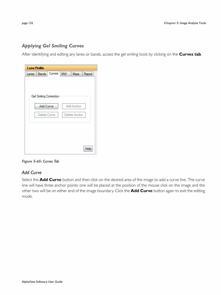
page 132 Chapter 5: Image Analysis Tools
Applying Gel Smiling Curves
After identifying and editing any lanes or bands, access the gel smiling tools by clicking on the Curves tab.
Figure 5-65: Curves Tab
Add CurveSelect the Add Curve button and then click on the desired area of the image to add a curve line. The curve line will have three anchor points: one will be placed at the position of the mouse click on the image and the other two will be on either end of the image boundary. Click the Add Curve button again to exit the editing mode.
AlphaView Software User Guide

Lane Profile page 133
Figure 5-66: Curve Line Added to the Image
To create the curve, click on any of the three yellow plus sign (+) anchors on the curve line and drag it to the desired position. When an anchor has been selected, it will change from a plus sign to a square.
Figure 5-67: Curve After Using Anchors to Adjust the Line
Once a curve has been added, the Adj. Rf values will update in the Data Table, and the following other Gel Smiling options are enabled:
AlphaView Software User Guide

page 134 Chapter 5: Image Analysis Tools
Figure 5-68: Curve Options
Adding and Deleting AnchorsAnchor points can be added by selecting the Add Anchor button. Roll the mouse to the area of the curve where the new anchor should be placed. The cursor will change to a plus sign in areas where an anchor can be added. Click on the curve to add the anchor. Click the Add Anchor button again to exit the editing mode.
Additionally, anchor points can be deleted by selecting the Delete Anchor button. Click once on an existing anchor to delete it. Click the Delete Anchor button again to exit the editing mode. To delete anchors when not in editing mode, simply click on the anchor and select the Delete key on the keyboard.
Delete CurveA curve can be deleted by selecting the Delete Curve button. Click on an existing curve to delete it. Click the Delete Curve button again to exit the editing mode. To delete curves when not in editing mode, simply click on the curve and select the Delete key on the keyboard.
Additional Gel Smiling CurvesAdd enough curves to properly mimic the curvature of the sample. The more curves applied, the more accu-rate calculations will be for molecular weight and band matching. After the initial curve is applied the software will attempt to mimic the curvature of the surrounding curves when new curves are applied. This results in less editing of the additional curves.
AlphaView Software User Guide
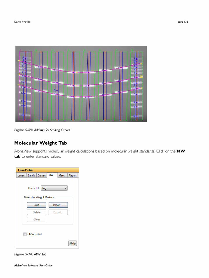
Lane Profile page 135
Figure 5-69: Adding Gel Smiling Curves
Molecular Weight Tab
AlphaView supports molecular weight calculations based on molecular weight standards. Click on the MW tab to enter standard values.
Figure 5-70: MW Tab
AlphaView Software User Guide

page 136 Chapter 5: Image Analysis Tools
Curve Fit
From the Curve Fit drop-down menu, select the molecular weight standards curve fitting option. The fit options are: log, linear, point to point fit, cubic spline and quadratic.
Import
To apply an existing set of molecular weight standard values select the Import button and select the desired *.mwm file.
NOTE: A set of preconfigured molecular weight standards files (*.mwm files) are installed with AlphaView software.
The molecular weight standards file can either be auto loaded or manually loaded.
Auto Load requires the user to select a lane to apply the molecular weight standard file. After the *.mwm file is selected, select YES to Auto Load. Roll the mouse over the image, the cursor will be a yellow line. When the yellow line is over the desired standard lane, click on the lane. AlphaView will automatically identify each band in the lane and associate it with a molecular weight standard in the imported file.
Figure 5-71: Molecular Weight Auto Load
Manual load requires the individual bands in a lane to be correlated manually with the standards in the imported file. After the *.mwm file is selected, select NO for Manual Load. Move the cursor to the first band of interest in a lane and click. Text at the top of the image will indicate how many molecular weight stan-dards are yet to be identified with a band selection, and what the molecular weight is. Continue to click on bands to identify molecular weight standards until all have been identified.
AlphaView Software User Guide

Lane Profile page 137
Figure 5-72: Molecular Weight Manual Load
Add Molecular Weight Marker
To identify a band as a molecular weight marker, select the Add button. Click on the first band in the known standard lane of the image. Enter the marker weight in the dialog box, then click OK.
Figure 5-73: Add Molecular Weight Dialog Box
Continue adding markers until all bands are identified. Click the Add button again to exit the editing mode.
Delete Molecular Weight Marker
To delete a molecular weight marker, select the Delete button. Move the cursor to the band in the image and click to delete it. Click the Delete button again to exit the editing mode.
AlphaView Software User Guide

page 138 Chapter 5: Image Analysis Tools
Clear Molecular Weight Markers
To clear all molecular weight markers in a lane, select the Clear button. Roll the mouse over the image. The cursor will be a yellow line. When the yellow line is over the desired lane, click on the lane. Once this is done, all molecular weight marker information in the lane will be removed. Click the Clear button again to exit the editing mode.
Molecular Weight Standards Results Display
After molecular weight standards have been identified, they will be color coded green in the Data Table. The curve fit used to calculate results will also be displayed below the Data Table.
Figure 5-74: Molecular Weight Standards Results Display
The calculated molecular weight for each band in the sample will now be displayed in the Calc MW column in the Data Table:
Figure 5-75: Calculated Sample Molecular Weight
Export
The set of molecular weight standards used for analysis can be saved for future use. To do this, click the Export button. A save dialog box will appear. Enter the name of the file and change the directory location if desired. If there are molecular weight standards in more than one lane, a lane must first be selected. To do this, roll the mouse over the image and move the yellow line cursor to the lane that contains the markers of interest. Click on the lane and save the file.
AlphaView Software User Guide

Lane Profile page 139
Show Molecular Weight Standard Curve
Select the Show Curve checkbox to display the molecular weight standards curve as calculated by the soft-ware. When this box is checked, the plot will be displayed in the lower right hand corner of the software win-dow.
Figure 5-76: Molecular Weight Standard Curve
Mass Standards
AlphaView supports mass calculations based on mass standards. Click on the Mass tab to enter individual mass standards or apply the total mass for a molecular ladder.
AlphaView Software User Guide
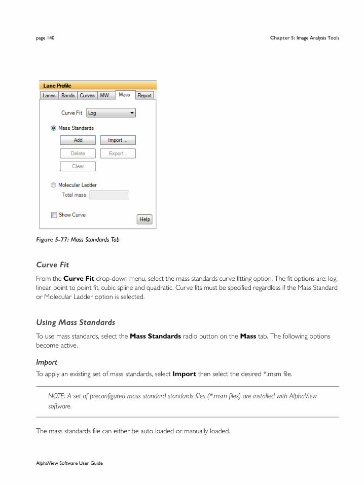
page 140 Chapter 5: Image Analysis Tools
Figure 5-77: Mass Standards Tab
Curve Fit
From the Curve Fit drop-down menu, select the mass standards curve fitting option. The fit options are: log, linear, point to point fit, cubic spline and quadratic. Curve fits must be specified regardless if the Mass Standard or Molecular Ladder option is selected.
Using Mass Standards
To use mass standards, select the Mass Standards radio button on the Mass tab. The following options become active.
ImportTo apply an existing set of mass standards, select Import then select the desired *.msm file.
NOTE: A set of preconfigured mass standard standards files (*.msm files) are installed with AlphaView software.
The mass standards file can either be auto loaded or manually loaded.
AlphaView Software User Guide
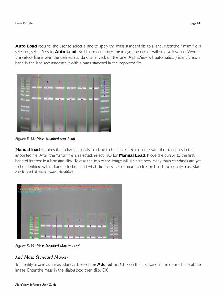
Lane Profile page 141
Auto Load requires the user to select a lane to apply the mass standard file to a lane. After the *.msm file is selected, select YES to Auto Load. Roll the mouse over the image, the cursor will be a yellow line. When the yellow line is over the desired standard lane, click on the lane. AlphaView will automatically identify each band in the lane and associate it with a mass standard in the imported file.
Figure 5-78: Mass Standard Auto Load
Manual load requires the individual bands in a lane to be correlated manually with the standards in the imported file. After the *.msm file is selected, select NO for Manual Load. Move the cursor to the first band of interest in a lane and click. Text at the top of the image will indicate how many mass standards are yet to be identified with a band selection, and what the mass is. Continue to click on bands to identify mass stan-dards until all have been identified.
Figure 5-79: Mass Standard Manual Load
Add Mass Standard MarkerTo identify a band as a mass standard, select the Add button. Click on the first band in the desired lane of the image. Enter the mass in the dialog box, then click OK.
AlphaView Software User Guide
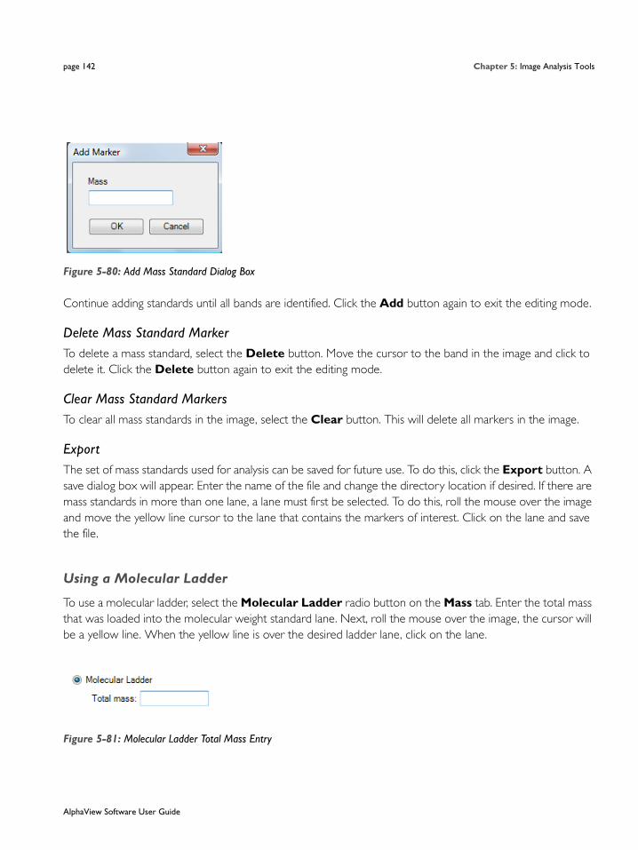
page 142 Chapter 5: Image Analysis Tools
Figure 5-80: Add Mass Standard Dialog Box
Continue adding standards until all bands are identified. Click the Add button again to exit the editing mode.
Delete Mass Standard MarkerTo delete a mass standard, select the Delete button. Move the cursor to the band in the image and click to delete it. Click the Delete button again to exit the editing mode.
Clear Mass Standard MarkersTo clear all mass standards in the image, select the Clear button. This will delete all markers in the image.
ExportThe set of mass standards used for analysis can be saved for future use. To do this, click the Export button. A save dialog box will appear. Enter the name of the file and change the directory location if desired. If there are mass standards in more than one lane, a lane must first be selected. To do this, roll the mouse over the image and move the yellow line cursor to the lane that contains the markers of interest. Click on the lane and save the file.
Using a Molecular Ladder
To use a molecular ladder, select the Molecular Ladder radio button on the Mass tab. Enter the total mass that was loaded into the molecular weight standard lane. Next, roll the mouse over the image, the cursor will be a yellow line. When the yellow line is over the desired ladder lane, click on the lane.
Figure 5-81: Molecular Ladder Total Mass Entry
AlphaView Software User Guide

Lane Profile page 143
Mass Standards Results DisplayAfter mass standards have been identified, they will be color coded green in the Data Table. The curve fit used to calculate results will also be displayed below the Data Table.
Figure 5-82: Mass Standards Results Display
The calculated mass for each band in the sample will now be displayed in the Calc. Mass column in the Data Table:
Figure 5-83: Calculated Sample Mass
Show Mass Standards CurveSelect the Show Curve checkbox to display the mass standards curve as calculated by the software. When this box is checked, the plot will be displayed in the lower right hand corner of the software window.
Figure 5-84: Mass Standard Curve
AlphaView Software User Guide

page 144 Chapter 5: Image Analysis Tools
Advanced Lane Profile Options
Lane Profile also includes two advanced options: Band Scoring and Band Matching. To view these options, they must be selected in Preferences. To do this, select Setup and Preferences from the Main Menu. Go to the Analysis Tools tab and select the Lane Profile - Advanced checkbox and click Apply.
Figure 5-85: Preferences Analysis Tools Tab
Lane Profile will now display two new tabs for each of the advanced options.
Band Scoring Tab
To perform band scoring, select the Scoring tab.
AlphaView Software User Guide

Lane Profile page 145
Figure 5-86: Band Scoring Tab
Lane #’s to score: Choose the lanes to score by highlighting the lanes to be included.
Score based on: Select the parameter to base the scoring on. The choices are Area, Mass, and Height. The Area and Height are calculated automatically in Lane Profile. In order to use the Mass as the scoring parameter the user must calculate the Mass of every band by applying a Mass Standard. This can be done sep-arately or in conjunction with MW calculations.
Select Scoring Method: Select the scoring method of interest. The choices are: Present/Absent; High/Medium/Low/Absent; % of control; and Quantity.
• Present/Absent: this method is used as a qualitative measurement for review. The researcher is interested in whether or not a lane has a specific band of interest based on some criteria (area, mass, or height).
• Additional Criteria: When choosing Present/Absent as the scoring method the user must enter a value for determining the presence or absence. The value is a percent. When the value of an unknown band falls below that percentage value it is classified as Absent, when it exceeds the value it is classified as Present.
• High/Medium/Low/Absent: This method is used to classify bands into groups based on Area, Mass, or Height. The researcher will determine break points for each classification (high, medium, low, and absent). The software will place each band into one of these classifications depending on the user entered criteria.
AlphaView Software User Guide

page 146 Chapter 5: Image Analysis Tools
• Additional Criteria: When choosing the High/Medium/Low/Absent method the user must enter in values to use as break points for each of these classifications. The values entered are percentages of the reference band based on the parameter chosen in the “score based on” field.
Figure 5-87: Band Scoring - Select Scoring Method
Band Matching, Similarity Matrix, and Dendrograms
AlphaView provides features for matching bands between lanes. The resultant data can then be used to gen-erate similarity matrices and/or dendrograms. Band matching features are accessible under the Analysis menu within Lane Profile’s Auto Lane feature.
Prerequisites for Band MatchingPrior to performing band matching, a number of steps must be followed:
1. Lanes and Bands must be detected and edited through the Auto Lane feature.
2. If Molecular Weights are to be calculated, molecular weight markers must be loaded prior to band matching. For more information, please refer to “Molecular Weight Tab” on page 135.
3. (Optional) A new Gel Smiling tool has been added to AlphaView. This tool allows the user to adjust the software’s calculations for M.W., Adj. Rf, and Band Matching by drawing the shape of the gel smile or cur-vature. Applying the Gel Smiling tool will aid in the accuracy of automatically matching bands and will result in less user edits afterwards. Refer to the section on Gel Smiling tool for further instructions.
AlphaView Software User Guide

Lane Profile page 147
Band Matching Band Matching dialog window is accessible through the Analysis menu on the Auto Lane’s Profile and Data window. Select Band Matching from the Analysis menu.
Figure 5-88: Band Matching Tab
Functionality is provided for both Automatic and Manual band matching. Each will be explained in detail.
NOTE: These are not exclusive. After Automatic Band Matching has been performed the user is able to use the Manual matching features to edit or correct the automatic findings.
Automatic Band Matching
Matching Metric
Select either Adjusted Rf Matching or Generic Rf Matching as the matching metric.
• Adjusted Rf Matching: When Adjusted Rf Matching is selected the software will match bands based on the data values in the Adjusted Rf column of the Profile and Data window. These values result from the gel smile/curvature rather than the absolute vertical Rf value. Adjusted Rf is calculated based on the addition of M.W. markers and/or the Rf Curve lines which serve to correct the Generic Rf values for gel smiling.
AlphaView Software User Guide

page 148 Chapter 5: Image Analysis Tools
• Generic Rf Matching: When Generic Rf Matching is selected the software will match bands based on the data values in the Rf column of the Profile and Data window. These values are the relative Rf calculated vertically where the origin of the lane is set to zero and the lane front is set to 1. Gel smiling or curvature is not adjusted for in this selection.
Matching Reference
Select a lane to serve as the matching reference. It is advised that you choose a lane that either contains most of the bands of interest or spans the range of bands of interest while also containing many of the bands of interest. This will reduce the amount of effort required for post match edits.
Matching Tolerance
Enter a value to be used as the matching tolerance. The tolerance is converted into the amount of displace-ment two bands may have and still be matched by the software. The larger the tolerance value the larger the range the software will use for matching. The valid range is 0-10%. A value of 1-5% typically works best. A lower percentage works well for tightly spaced bands.
Auto Match
After selecting a matching metric, reference, and tolerance click the Auto Match button for the software to perform auto matching. When matching has been completed the Display Results and Generate Dendrogram buttons will become active. Refer to the appropriate sections below for a description of Similarity Results and Dendrogram creation.
Editing Match Results
Following Automatic band matching the user may need to manually edit or correct some matches. The tools under Manual Matching can be used for this purpose. Refer to the section below on Manual Matching for a description of each tool.
Manual Band Matching
Manual band matching tools are useful for quickly matching lanes with only a few bands or for manual edits and corrections to Automatic Band Matching results.
AlphaView Software User Guide

Lane Profile page 149
Figure 5-89: Band Matching Tab
New Band Type
Select the New Band Type tool by clicking the New Band Type button. A Band Type is a band with a unique Rf. or Adj. Rf. Value. Each band within a lane will be part of a band type and no two bands within a lane can be of the same band type.
After selecting the New Band Type tool, click on a band to draw a band type line. Repeat this process of selecting the tool and clicking a band until a band for each unique band type has been selected.
Deleting a Band Type
To delete a band type, select the Delete Band Type button and click on a band type line.
Adding Bands to a Band Type
Select the Plus Band tool by clicking the Plus Band button. Click on a band type line to select it, the line will be highlighted in yellow. Now click on a band that belongs to this band type. Repeat this process for all bands belonging to this band type. Then repeat the process for each band type until all bands have been identified as belonging to a band type.
Removing Bands from a Band Type
Select the Minus Band tool by clicking on the Minus Band button. Click on a band type line to select it, the line will be highlighted in yellow. Now click on the band that you would like to remove from the selected band type.
AlphaView Software User Guide
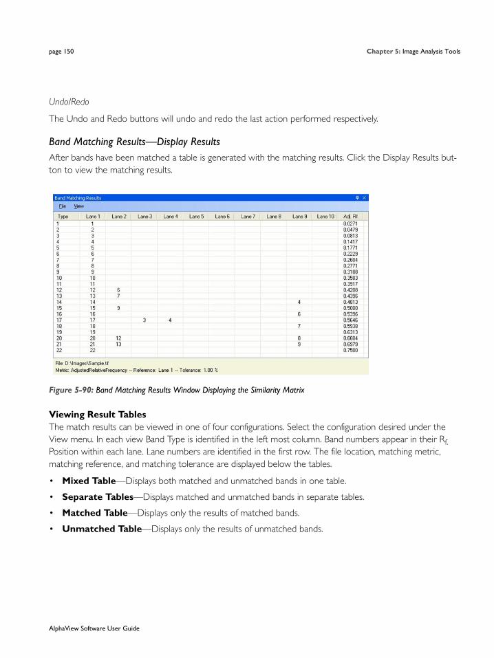
page 150 Chapter 5: Image Analysis Tools
Undo/Redo
The Undo and Redo buttons will undo and redo the last action performed respectively.
Band Matching Results—Display ResultsAfter bands have been matched a table is generated with the matching results. Click the Display Results but-ton to view the matching results.
Figure 5-90: Band Matching Results Window Displaying the Similarity Matrix
Viewing Result TablesThe match results can be viewed in one of four configurations. Select the configuration desired under the View menu. In each view Band Type is identified in the left most column. Band numbers appear in their Rf. Position within each lane. Lane numbers are identified in the first row. The file location, matching metric, matching reference, and matching tolerance are displayed below the tables.
• Mixed Table—Displays both matched and unmatched bands in one table.
• Separate Tables—Displays matched and unmatched bands in separate tables.
• Matched Table—Displays only the results of matched bands.
• Unmatched Table—Displays only the results of unmatched bands.
AlphaView Software User Guide
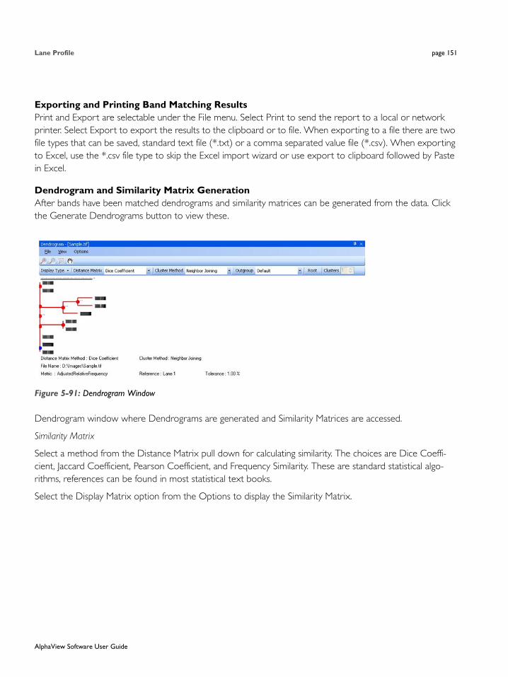
Lane Profile page 151
Exporting and Printing Band Matching ResultsPrint and Export are selectable under the File menu. Select Print to send the report to a local or network printer. Select Export to export the results to the clipboard or to file. When exporting to a file there are two file types that can be saved, standard text file (*.txt) or a comma separated value file (*.csv). When exporting to Excel, use the *.csv file type to skip the Excel import wizard or use export to clipboard followed by Paste in Excel.
Dendrogram and Similarity Matrix GenerationAfter bands have been matched dendrograms and similarity matrices can be generated from the data. Click the Generate Dendrograms button to view these.
Figure 5-91: Dendrogram Window
Dendrogram window where Dendrograms are generated and Similarity Matrices are accessed.
Similarity Matrix
Select a method from the Distance Matrix pull down for calculating similarity. The choices are Dice Coeffi-cient, Jaccard Coefficient, Pearson Coefficient, and Frequency Similarity. These are standard statistical algo-rithms, references can be found in most statistical text books.
Select the Display Matrix option from the Options to display the Similarity Matrix.
AlphaView Software User Guide

page 152 Chapter 5: Image Analysis Tools
Figure 5-92: Similarity Matrix
The similarity matrix is a graphical display of the similarity between lanes.
Exporting and Printing the Similarity Matrix
Print and Export are selectable under the File menu. Select Print to send the report to a local or network printer. Select Export to export the results to the clipboard or to file. When exporting to a file there are two file types that can be saved, standard text file (*.txt) or a comma separated value file (*.csv). When exporting to Excel, use the *.csv file type to skip the Excel import wizard or use export to clipboard followed by Paste in Excel.
DendrogramsThe dendrogram window is accessed by clicking the Generate Dendrograms button in the Band Matching dia-log.
Figure 5-93: Dendrograms
AlphaView Software User Guide
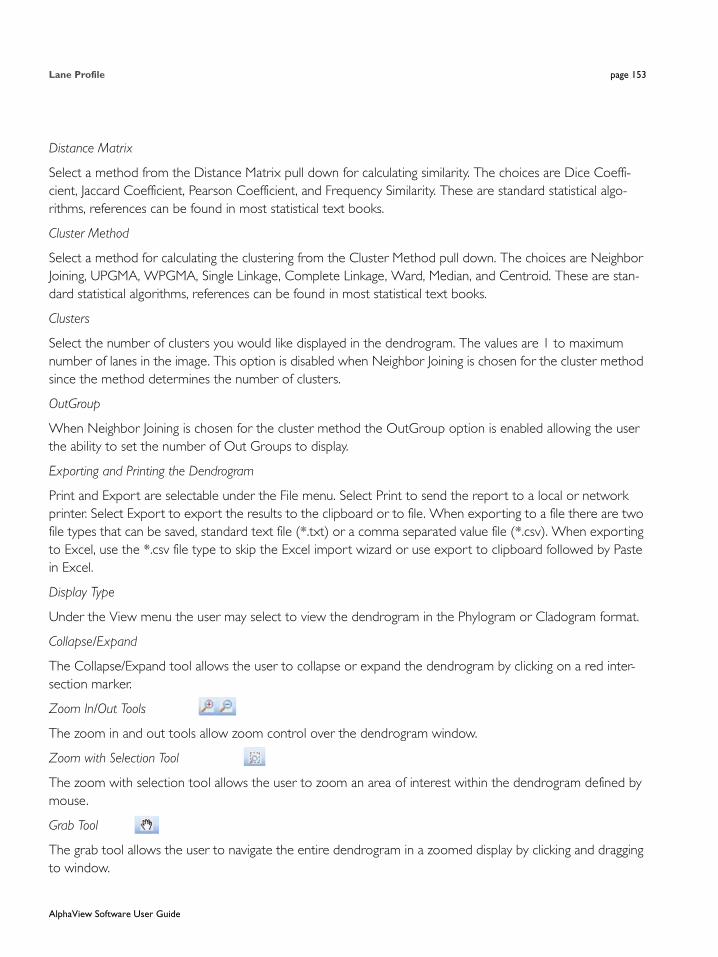
Lane Profile page 153
Distance Matrix
Select a method from the Distance Matrix pull down for calculating similarity. The choices are Dice Coeffi-cient, Jaccard Coefficient, Pearson Coefficient, and Frequency Similarity. These are standard statistical algo-rithms, references can be found in most statistical text books.
Cluster Method
Select a method for calculating the clustering from the Cluster Method pull down. The choices are Neighbor Joining, UPGMA, WPGMA, Single Linkage, Complete Linkage, Ward, Median, and Centroid. These are stan-dard statistical algorithms, references can be found in most statistical text books.
Clusters
Select the number of clusters you would like displayed in the dendrogram. The values are 1 to maximum number of lanes in the image. This option is disabled when Neighbor Joining is chosen for the cluster method since the method determines the number of clusters.
OutGroup
When Neighbor Joining is chosen for the cluster method the OutGroup option is enabled allowing the user the ability to set the number of Out Groups to display.
Exporting and Printing the Dendrogram
Print and Export are selectable under the File menu. Select Print to send the report to a local or network printer. Select Export to export the results to the clipboard or to file. When exporting to a file there are two file types that can be saved, standard text file (*.txt) or a comma separated value file (*.csv). When exporting to Excel, use the *.csv file type to skip the Excel import wizard or use export to clipboard followed by Paste in Excel.
Display Type
Under the View menu the user may select to view the dendrogram in the Phylogram or Cladogram format.
Collapse/Expand
The Collapse/Expand tool allows the user to collapse or expand the dendrogram by clicking on a red inter-section marker.
Zoom In/Out Tools
The zoom in and out tools allow zoom control over the dendrogram window.
Zoom with Selection Tool
The zoom with selection tool allows the user to zoom an area of interest within the dendrogram defined by mouse.
Grab Tool
The grab tool allows the user to navigate the entire dendrogram in a zoomed display by clicking and dragging to window.
AlphaView Software User Guide

page 154 Chapter 5: Image Analysis Tools
Common Features
Default analysis tool has three common features namely, Protocol, Report, and Export Results.
Protocol
Figure 5-94: Protocol Tab
The Protocol tab is used to save and load protocols for use on replicate blots.
Saving a protocol differs from saving an analysis in that protocols may be used on images other than the orig-inal image while a saved analysis is available for loading only on the original image.
NOTE: An analysis may be saved at anytime by using the file drop down menu.
Figure 5-95: Saving an Analysis
AlphaView Software User Guide

Lane Profile page 155
A protocol or analysis contains all band and background regions created with the loading controls, band con-trols and standard curve settings used. A protocol or analysis may be saved at any point in the analysis work-flow.
Report
Using Report Tab, user can generate reports based on analysis data. Reports offers different options to cus-tomize the report, which can be saved on file as an Html Format (*.html) or Rich Text Format (*.rtf). User can also take print of report.
Reports also allows user to save report settings/configuration as template or can modify existing templates.
FormattingFormatting tab allows user to format reports before saving or sending it to printer.
User can create new report or select existing report template to create a report using the drop down list. If no report template is defined/saved, it will be disabled.
Choose image that will be part of report with the image size. 1/4 is the default image size.
Also choose different information (Data sheet, Graph, Acquisition information) that will be part of report.
Report settings/configuration can be saved using Save button, in case of new or Save as in case of modifying an existing report template.
Figure 5-96: Report – Formatting Tab
AlphaView Software User Guide
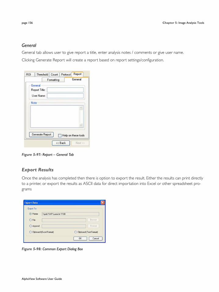
page 156 Chapter 5: Image Analysis Tools
GeneralGeneral tab allows user to give report a title, enter analysis notes / comments or give user name.
Clicking Generate Report will create a report based on report settings/configuration.
Figure 5-97: Report – General Tab
Export Results
Once the analysis has completed then there is option to export the result. Either the results can print directly to a printer, or export the results as ASCII data for direct importation into Excel or other spreadsheet pro-grams
Figure 5-98: Common Export Dialog Box
AlphaView Software User Guide

Lane Profile page 157
Sending Data to a PrinterTo send the data directly to the Video Printer or Default Printer, click on the Export button and click in the circle next to appropriate printer.
Sending Data to a FileIf you would like to take the data from the system and import it into another computer, the data can be saved to a diskette or network which will allow you to open the data file on a separate workstation connected to the network.
Click on the Export button and then on the File option. Specify the path and file name to send the data file. The data is saved as an ASCII file and can be imported into most spreadsheet programs. ASCII is a very common file format output option for numerical data.
Appending Data to a Same FileExport dialog also allows you to append data to an existing exported file.
NOTE: This feature is applicable to AutoCount and Array analysis modules.
Sending Data to a Spreadsheet ProgramTo send the data results to Excel or other spreadsheet programs, click on the Export button, click on the clip-board option, then click on OK. If you have Excel or another spreadsheet program loaded on the system and running in the background, you can simply press the ALT and TAB keys simultaneously to move into the spreadsheet program. You can then import the data directly to the desired spreadsheet from clipboard.
NOTE: The spreadsheet program must be installed on the computer in order to export the data to that program.
When the appropriate export source has been selected, click on the OK button to send the data.
Exporting Quantitative Data Lane ProfileThe exporting of Lane Profile is similar to what has been defined above with some extra feature.
The Lane Profile has following window to export data.
AlphaView Software User Guide

page 158 Chapter 5: Image Analysis Tools
Figure 5-99: Lane Profile Export Dialog Box
Output LaneThis option allows user to export what type of data to be exported. Selecting All Lanes will export all lanes data or selecting Current Lane will only export current lane data.
To send the data, click on the OK button.
Additional Analysis Tools
Figure 5-100: Additional Analysis Tools in the ToolBox
Additional image analysis tools can be activated to show up under the tool box as shown here. To activate these tools:
1. Go to Setup> Preferences > Analysis tools tab.
2. Select tools to show.
AlphaView Software User Guide

Additional Analysis Tools page 159
Figure 5-101: Preferences—Analysis Tools Tab
This tool set allows the user to perform ruler measurements, gel scoring, manual counting of colonies and cells, and perform high density array analysis.
The Ruler Function
The Ruler function allows the user to create a scale based on a standard and to measure distances from a set origin to a chosen location.
Figure 5-102: The Ruler Tools and Ruler Toolbox
AlphaView Software User Guide

page 160 Chapter 5: Image Analysis Tools
Using the Ruler Function
To access the Ruler function, click on ToolBox, Analysis Tools and then on Ruler. A line with a box at each end and a circle with a cross in it will appear on the screen.
Before any measurements can be obtained, a standard scale must be established. The scale that is created will serve as the standard for all measurements. Therefore, it is advisable to draw the scale line according to some standard measurement within the image (such as a ruler).
Using the mouse, click and drag one end of the line and then the other end into position. Once the line is in position, click in the Scale Length box and type the length of the standard. Press <enter> to save this value.
Distance is measured from the origin (designated by the circle with a cross in it) to the mouse location. Place the origin marker appropriately, and then move the mouse. The distance will be constantly updated in the Distance box.
To hide the scale and origin, click on the Hide Origin Scale checkbox.
Cartesian CoordinatesThe Ruler function can also be used to create a Cartesian coordinate system. The origin icon has default val-ues (0.000, 0.000). These can be changed by clicking on the Origin box, typing in new values, and clicking <enter>.
Once the origin is placed on the screen in its desired location, the relative coordinates of the mouse at any location are shown at the right-hand side of the screen. In the example above, the cursor is 0.747 inches to the right of the origin and 1.071 inches below. To hide the coordinates, click on the Hide Coordinates checkbox.
The Scoring Function
The Scoring function is designed for gene expression applications to check for presence or absence of specific samples. The scoring function can be used for a quick manual identification of several different sample types. The software allows for up to three different scores on a gel, blot, or microtiter plate.
To score an image, click on the Scoring button in Toolbox 4. Define the appropriate number of rows and col-umns of your image by using the appropriate controls. You can also define the amount of spacing between your rows and columns to compensate for any variations between lanes or wells.
AlphaView Software User Guide

Additional Analysis Tools page 161
Figure 5-103: Scoring Controls
Once you have selected the number of rows and columns to be displayed, you may adjust the template to fit your image. Use the left button on the mouse to click, hold, and drag the outside borders of the template so they frame the lanes or wells to be scored. Clicking, holding, and dragging on or within any border moves the entire template. Clicking on the blue corners surrounding the template resizes it.
Figure 5-104: Scoring Image with Template Positioned
Scoring the Sample
Three different scoring options are available: score with a positive, negative, or positive / negative. The soft-ware will display an “X” if you have a positive sample or three “–“ signs arranged in a vertical fashion if you score with a negative. Nothing will appear if you score with a positive/negative. You may use the right and left mouse buttons to determine different scores. The right mouse button will score the sample with an “X”. The left mouse button will score the sample with three “-“ signs vertically arranged.
AlphaView Software User Guide

page 162 Chapter 5: Image Analysis Tools
Figure 5-105: Scoring for positives (+), negatives (-), and positive / negative (nothing)
For faster scoring, you may look at the entire image and visually determine whether the samples are primarily positive, negative, or positive / negative. By clicking on the All +, All -, or All +/- boxes, all of the samples on the image will have either an “X”, three “-”, or nothing depending on the button you clicked.
Figure 5-106: Image after All+ button pressed vs. Image after All+ button Pressed and Individual Sample Scoring
Figure 5-107: Output and Scoring Options
Manual Count
Click on Manual Count. The following sets of tools will be displayed in the lower left of the screen. Some samples are extremely difficult to count because of their shape, size, or lack of intensity variation from the background. To accurately count these samples, we have developed the manual counting feature within our software. To manually count the objects in an image, click on Manual Count in Tool Box, Analysis Tools. You may use either a green x or a red +. If you are only counting one type of sample, you may simply use the x which is the default to begin counting in the software.
AlphaView Software User Guide

Additional Analysis Tools page 163
Figure 5-108: Manual Count Tools
Placing Markers to Count
Point the cursor at an object to be counted and click the left mouse button. An “x” is placed over the object, ensuring that the same object will not be mistakenly counted twice. In the toolbox, the number in the Count box automatically increases by 1. Click on all of the objects of this type or color to be counted.
To count objects of another type or color (such as white vs. blue colonies in a β-gal assay), use right mouse button to click on each object as above.
Figure 5-109: Section of an Image After Manual Counting and Corresponding Data
Erasing and Hiding Count Markers
To erase a marker that has been manually placed, click on the marker on the image. It will disappear and the count will be reduced by one.
The Sensitivity indicator determines how close the cursor must be to a marker in order to delete it. Higher numbers allow the user to click further away from the marker to delete it; however, if Sensitivity is set too high, it will be impossible to place markers on spots that are close together.
AlphaView Software User Guide
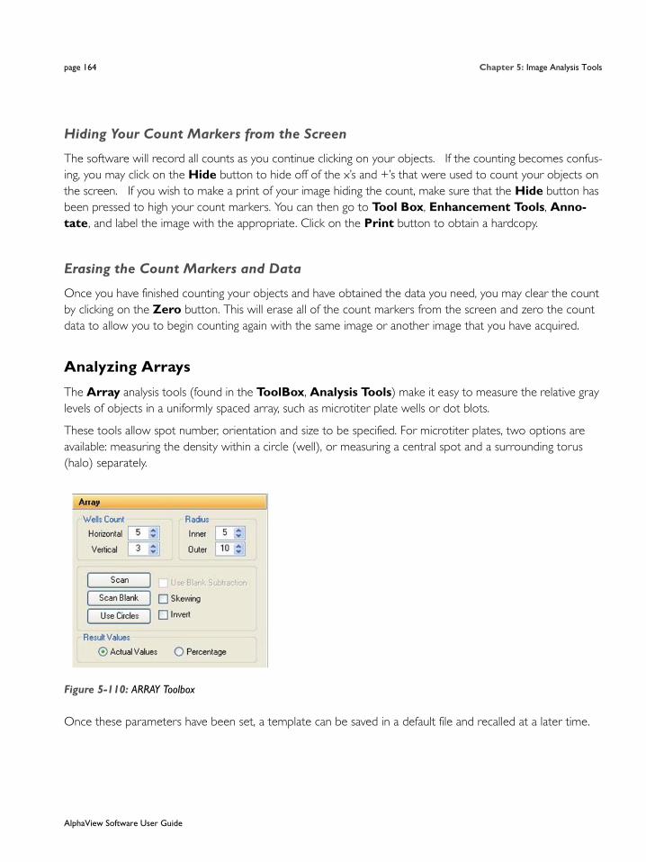
page 164 Chapter 5: Image Analysis Tools
Hiding Your Count Markers from the Screen
The software will record all counts as you continue clicking on your objects. If the counting becomes confus-ing, you may click on the Hide button to hide off of the x’s and +’s that were used to count your objects on the screen. If you wish to make a print of your image hiding the count, make sure that the Hide button has been pressed to high your count markers. You can then go to Tool Box, Enhancement Tools, Anno-tate, and label the image with the appropriate. Click on the Print button to obtain a hardcopy.
Erasing the Count Markers and Data
Once you have finished counting your objects and have obtained the data you need, you may clear the count by clicking on the Zero button. This will erase all of the count markers from the screen and zero the count data to allow you to begin counting again with the same image or another image that you have acquired.
Analyzing Arrays
The Array analysis tools (found in the ToolBox, Analysis Tools) make it easy to measure the relative gray levels of objects in a uniformly spaced array, such as microtiter plate wells or dot blots.
These tools allow spot number, orientation and size to be specified. For microtiter plates, two options are available: measuring the density within a circle (well), or measuring a central spot and a surrounding torus (halo) separately.
Figure 5-110: ARRAY Toolbox
Once these parameters have been set, a template can be saved in a default file and recalled at a later time.
AlphaView Software User Guide

Additional Analysis Tools page 165
Setting Up an Array Template
To access the Array tools, open ToolBox, Analysis Tools and click on the Array button. A template is displayed on the image, depicting the layout of the objects to be measured. Up to 10,000 objects in a 100x100 array can be measured. (The default is an array of 96 circles, arranged in 8 rows of 12.)
Figure 5-111: ARRAY Template
The tool box work area displays a number of buttons and controls for specifying the number of objects, along with their orientation and sizes.
Analyze Arrays with Circles or Squares
Figure 5-112: Array Dialog Box
AlphaView Software User Guide

page 166 Chapter 5: Image Analysis Tools
The controls labeled Hori. Wells and Ver. Wells let the number of horizontal and vertical objects be set (to a maximum of 100 and 100, respectively). The controls labeled Center and Outer let the size of the center and outer circles be set. Click on an arrow to increase or decrease the number of objects per row or column, or the size of the objects. As the number and size are adjusted, the template displayed over the image is updated to reflect the changes.
Aligning the Template
Once the number of objects has been set, adjust the placement of the template.
If the image of the sample is not parallel with the template, the template can be realigned by adjusting the green line so it is parallel to the top edge of the sample. Place the cursor on the box at either end of the line. Hold the left mouse button down and drag the line until it is parallel to the image.
Next, adjust the placement of the template so the objects coincide with the areas of interest on the image. Move the cursor to any of the square “handles” on the outside of the template. Hold down the left mouse button and drag the handles until the template is properly positioned.
If the image is not perfectly rectangular, the template can be skewed by clicking the Skewing checkbox.
Figure 5-113: A Skewed Template
AlphaView Software User Guide

Additional Analysis Tools page 167
Specifying the Areas to Be Measured
For microtiter plate analysis, the toolbox controls labeled Center and Outer specify the size of the inner circle and outer torus scanned to measure each well. The number in the center of each of these controls indicates the diameter of the circles. Click on an arrow to increase or decrease the diameters. As the number is adjusted, the objects on the template grow larger or smaller, reflecting the changes.
When specifying the size of the area to be measured, exclude shadows or other imaging artifacts. Depending upon the lighting conditions when the image was captured, there may be a crescent-shaped shadow obscur-ing part of the bottom of the wells, especially those near the edge of the microtiter plate. We recommend decreasing the size of the sampling area so that these regions are not included.
To measure the total density within each object, reduce the Center value to zero (0) and adjust the Outer value until the objects on the screen are slightly smaller than the areas of interest on the image. Reposition the corner objects using the mouse until the objects are properly aligned over the objects.
Measuring Density
Once the objects are sized and positioned correctly, click on the Scan button in the tool box. The density values will be calculated and displayed under each object.
The values are the average pixel values within the object, adjusted to a scale of 0 to 100. (0 corresponding to black pixel values, and 100 corresponding to white pixel values.)
If both a center and an outer circle have been specified, two values are displayed. The upper value corre-sponds to the inner circle and the lower value corresponds to the torus.
The Invert Box
The Invert function reverses the relative density assignments so that 0 corresponds to white and 100 corre-sponds to black. If the image has dark areas of interest on a light background, then Invert should be selected by placing an “X” in its box. (If the image has light areas of interest on a dark background, the Invert option should not be activated.) Unlike the Reverse option described in “The Reverse Button” on page 10, this function does not alter the appearance of the image.
Removing Background Using the Scan Blank Function
Since a microtiter plate is not completely transparent, it contributes to the density measured when samples are scanned. A non-uniform light source also affects the density measured. To ensure that the density mea-sured is attributable only to the sample in the wells, scan a “blank” before scanning samples.
Load an image of a clean, unused microtiter plate and align the objects as described above. Once the array has been set up, click on the Scan Blank button. The average pixel gray value for each object (and torus) is measured and set to zero (0).
AlphaView Software User Guide

page 168 Chapter 5: Image Analysis Tools
Now, when samples are scanned, the gray value of the blank is subtracted from that of the sample before it is scaled. This ensures that the density reported only reflects the sample in each well.
When Scan Blank has been selected, the background values obtained apply to all subsequent scans. To indi-cate that a background is being applied, the Scan Blank button changes to read Clear Blank. To turn off this background subtraction function, simply click on Clear Blank.
Lane Profile - Advanced
When the Lane Profile - Advanced checkbox is selected, Band Scoring and Band Matching tabs are added to the Lane Profile options in the Analysis Tools tab of the Toolbox. For complete details, please see “Advanced Lane Profile Options” on page 144.
Common Export Result Feature
Once the analysis has completed then there is option to export the result. Either the results can print directly to a printer, or export the results as ASCII data for direct importation into Excel or other spreadsheet pro-grams
Figure 5-114: Common Export Dialog Box
Sending Data to a PrinterTo send the data directly to the Video Printer or Default Printer, click on the Export button and click in the circle next to appropriate printer.
Sending Data to a FileIf you would like to take the data from the system and import it into another computer, the data can be saved to a diskette or network which will allow you to open the data file on a separate workstation connected to the network.
Click on the Export button and then on the File option. Specify the path and file name to send the data file. The data is saved as an ASCII file and can be imported into most spreadsheet programs. ASCII is a very common file format output option for numerical data.
AlphaView Software User Guide

Additional Analysis Tools page 169
Appending Data to a Same FileExport dialog also allows you to append data to an existing exported file.
NOTE: This feature is applicable to AutoCount and Array analysis modules.
Sending Data to a Spreadsheet ProgramTo send the data results to Excel or other spreadsheet programs, click on the Export button, click on the clip-board option, then click on OK. If you have Excel or another spreadsheet program loaded on the system and running in the background, you can simply press the ALT and TAB keys simultaneously to move into the spreadsheet program. You can then import the data directly to the desired spreadsheet from clipboard.
NOTE: The spreadsheet program must be installed on the computer in order to export the data to that program.
When the appropriate export source has been selected, click on the OK button to send the data.
AlphaView Software User Guide

page 170 Chapter 5: Image Analysis Tools
AlphaView Software User Guide

page 171
Appendix A:
AlphaView Molecular Weight Library Files
Appendix Overview• List of Standards
AlphaView Software User Guide

page 172 Appendix A: AlphaView Molecular Weight Library Files
List of StandardsA library including the following DNA, RNA and protein molecular weight standards has been incorporated into AlphaView.
Values of size standards are given in base pairs.
Table A-1: AlphaQuant Standards
AlphaQuant 1
AlphaQuant 2
AlphaQuant 3
AlphaQuant 4
AlphaQuant 5
AlphaQuant 6
AlphaQuant 7
10000 2000 5000 1000 500 2000 5000
8000 1800 4500 800 400 1000 3000
6000 1600 4000 700 300 500 2000
5000 1400 3500 600 250 250 1000
4000 1200 3000 500 200 100 500
3000 1000 2500 400 175
2500 800 2000 300 150
2000 700 1500 200 125
1500 600 1000 100 100
1000 500 700 75
800 400 500 50
600 300 25
400 200
200 100
50
AlphaView Software User Guide

List of Standards page 173
Table A-2: DNA Sizing Standards
DNA Size Standards (in bp)
HINDIII PHIX174 BRL10BP BRL50BP BRL100BP PRO100BP BRL123BP BRL1KB BRLHIMW
23130 1353 200 500 1500 1500 4182 12216 48502
9416 1078 190 450 1400 1000 4059 11198 38416
6557 872 180 400 1300 900 3936 10180 33498
4361 603 170 350 1200 800 3813 9162 29942
2322 310 160 300 1100 700 3690 8144 24776
2027 281 150 250 1000 600 3567 7126 22621
564 271 140 200 900 500 3444 6108 19399
125 234 130 150 800 400 3321 5090 17057
194 120 100 700 300 3198 4072 15004
118 110 50 600 200 3075 3054 12220
72 100 500 100 2952 2036 10086
90 400 2829 1636 8612
80 300 2706 1018 8271
70 200 2583 517
60 100 2460 396
50 2337 344
40 2214 298
30 2091 220
20 1968 201
10 1845 154
1722 134
1599 75
1476
1353
1230
AlphaView Software User Guide

page 174 Appendix A: AlphaView Molecular Weight Library Files
Table A-3: RNA and Protein Standards
HINDIII PHIX174 BRL10BP BRL50BP BRL100BP PRO100BP BRL123BP BRL1KB BRLHIMW
1107
984
861
738
615
492
369
246
123
RNA Size Standards Protein Markers (in kD)
BRLRNA1 BRLRNA2 BRLPROT1 BRLPROT2 BRLPROT3 BRL10KD NOVEXM12 SIG-MAHMW
SIG-MAPMW
1770 9490 87.0 200.0 43.0 200 200.0 205 190
1520 7460 60.0 97.4 29.0 120 116.3 116 108
1280 4400 53.0 68.0 18.4 110 97.4 97 89
780 2370 46.0 43.0 14.3 100 66.3 84 77
530 1350 40.0 29.0 6.2 90 55.4 66 61
400 240 34.0 18.4 3.0 80 36.5 55 41
280 29.0 14.3 70 31.0 45 36
155 27.0 60 21.5 36
21.0 50 14.4
15.0 40 6.0
6.5 30 3.5
20 2.5
10
DNA Size Standards (in bp)
AlphaView Software User Guide
page 175
Appendix B:
Data Description Tables
Appendix Overview• Single Channel Columns
• Multichannel Columns
AlphaView Software User Guide

page 176 Appendix B: Data Description Tables
Single Channel Columns
Region Tab
Band Band Identifying Number
Sum Sum of all pixel gray levels in Band
Percentage (%) Percentage Sum =(Sum/ Total of all Band Sums)*100
Area Area of Band Region in pixels
Average Average pixel level of Band = (Sum/Area)
X Y Position XY position of Band Region centroid
SD Pixel Levels Standard Deviation of pixel gray levels in Band
Background Tab
BC Sum Background Corrected Sum = (BC Average *Area)
BC Average Background Corrected Average = (Average – Bkgd Average)
Note Subtracting the Bkgd Average from the Average accounts for differences in area
Bkgd Sum Sum of all pixel gray levels in Background Region
Bkgd Area Area of Background Region
Bkgd Average Average pixel level of Background region = (Bkgd Sum /Bkgd area)
Bkgd XY X Y position of Background region
Bkgd SD Standard deviation of pixel gray levels in background region
Signal/Noise Signal to Noise ratio of the band region = (Average– Bkgd Average) /Bkgd SD
Control Tab
LCN Sum Loading Control Normalized Sum = (LCN Average* Area)
LCN Average Loading Control Normalized Average = (BC Average of Experimental Band/BC Aver-age of corresponding Loading control) * mean of all loading controls.
NOTE: If a background correction has not been applied, Average is used.
AlphaView Software User Guide
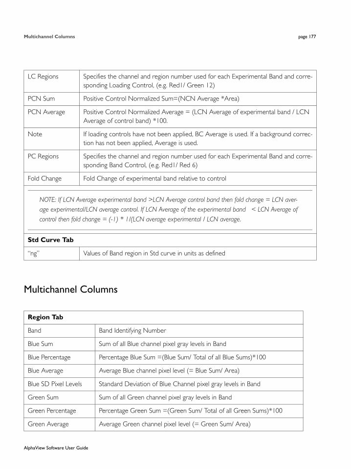
Multichannel Columns page 177
Multichannel Columns
LC Regions Specifies the channel and region number used for each Experimental Band and corre-sponding Loading Control, (e.g. Red1/ Green 12)
PCN Sum Positive Control Normalized Sum=(NCN Average *Area)
PCN Average Positive Control Normalized Average = (LCN Average of experimental band / LCN Average of control band) *100.
Note If loading controls have not been applied, BC Average is used. If a background correc-tion has not been applied, Average is used.
PC Regions Specifies the channel and region number used for each Experimental Band and corre-sponding Band Control, (e.g. Red1/ Red 6)
Fold Change Fold Change of experimental band relative to control
NOTE: If LCN Average experimental band >LCN Average control band then fold change = LCN aver-age experimental/LCN average control. If LCN Average of the experimental band < LCN Average of control then fold change = (-1) * 1/(LCN average experimental / LCN average.
Std Curve Tab
“ng” Values of Band region in Std curve in units as defined
Region Tab
Band Band Identifying Number
Blue Sum Sum of all Blue channel pixel gray levels in Band
Blue Percentage Percentage Blue Sum =(Blue Sum/ Total of all Blue Sums)*100
Blue Average Average Blue channel pixel level (= Blue Sum/ Area)
Blue SD Pixel Levels Standard Deviation of Blue Channel pixel gray levels in Band
Green Sum Sum of all Green channel pixel gray levels in Band
Green Percentage Percentage Green Sum =(Green Sum/ Total of all Green Sums)*100
Green Average Average Green channel pixel level (= Green Sum/ Area)
AlphaView Software User Guide
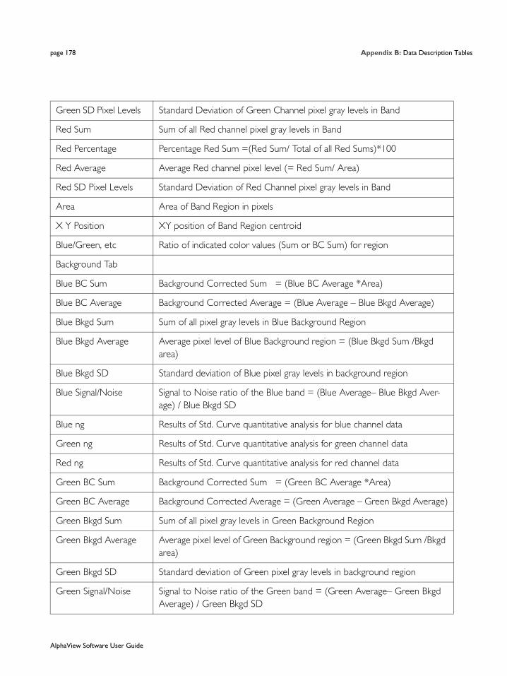
page 178 Appendix B: Data Description Tables
Green SD Pixel Levels Standard Deviation of Green Channel pixel gray levels in Band
Red Sum Sum of all Red channel pixel gray levels in Band
Red Percentage Percentage Red Sum =(Red Sum/ Total of all Red Sums)*100
Red Average Average Red channel pixel level (= Red Sum/ Area)
Red SD Pixel Levels Standard Deviation of Red Channel pixel gray levels in Band
Area Area of Band Region in pixels
X Y Position XY position of Band Region centroid
Blue/Green, etc Ratio of indicated color values (Sum or BC Sum) for region
Background Tab
Blue BC Sum Background Corrected Sum = (Blue BC Average *Area)
Blue BC Average Background Corrected Average = (Blue Average – Blue Bkgd Average)
Blue Bkgd Sum Sum of all pixel gray levels in Blue Background Region
Blue Bkgd Average Average pixel level of Blue Background region = (Blue Bkgd Sum /Bkgd area)
Blue Bkgd SD Standard deviation of Blue pixel gray levels in background region
Blue Signal/Noise Signal to Noise ratio of the Blue band = (Blue Average– Blue Bkgd Aver-age) / Blue Bkgd SD
Blue ng Results of Std. Curve quantitative analysis for blue channel data
Green ng Results of Std. Curve quantitative analysis for green channel data
Red ng Results of Std. Curve quantitative analysis for red channel data
Green BC Sum Background Corrected Sum = (Green BC Average *Area)
Green BC Average Background Corrected Average = (Green Average – Green Bkgd Average)
Green Bkgd Sum Sum of all pixel gray levels in Green Background Region
Green Bkgd Average Average pixel level of Green Background region = (Green Bkgd Sum /Bkgd area)
Green Bkgd SD Standard deviation of Green pixel gray levels in background region
Green Signal/Noise Signal to Noise ratio of the Green band = (Green Average– Green Bkgd Average) / Green Bkgd SD
AlphaView Software User Guide

Multichannel Columns page 179
Red BC Sum Background Corrected Sum = (Red BC Average *Area)
Red BC Average Background Corrected Average = (Red Average – Red Bkgd Average)
Red Bkgd Sum Sum of all pixel gray levels in Red Background Region
Red Bkgd Average Average pixel level of Red Background region = (Red Bkgd Sum /Bkgd area)
Red Bkgd SD Standard deviation of Red pixel gray levels in background region
Red Signal/Noise Signal to Noise ratio of the Red band = (Red Average– Red Bkgd Average) / Red Bkgd SD
Bkgd Area Area of Background Region
Bkgd XY X Y position of Background region
Control Tab
LCN Sum Loading Control Normalized Sum = (LCN Average* Area)
LCN Average Loading Control Normalized Average = (BC Average of Experimental Band/BC Average of corresponding Loading control) * mean of all loading controls.
LC Regions Specifies the channel and region number used for each Experimental Band and corresponding Loading Control, (e.g. Red1/ Green 12)
PCN Sum Positive Control Normalized Sum=(NCN Average *Area)
PCN Average Positive Control Normalized Average = (LCN Average of experimental band / LCN Average of control band) *100.
PC Regions Specifies the channel and region number used for each Experimental Band and corresponding Band Control, (e.g. Red1/ Red 6)
Fold Change Fold Change of experimental band relative to control
NOTE: If LCN Average experimental band > LCN Average control band then fold change = LCN average experimental / LCN average control. If LCN Average of the experimental band < LCN Average of control then fold change = (-1) * 1/(LCN average experimental / LCN average.
AlphaView Software User Guide

page 180 Appendix B: Data Description Tables
AlphaView Software User Guide

page 181
Appendix C:
Data Interpretation
Appendix Overview• Loading Controls
AlphaView Software User Guide

page 182 Appendix C: Data Interpretation
Loading ControlsIn a typical Western blot experiment, the expression levels of one or more experimental proteins are analyzed to determine the effects of various treatments or conditions. The appropriate controls must be included on westerns blots as a number of factors can influence the proper interpretation of the signal levels extracted from multicolor images especially when comparing signal levels from different color channels.
A loading control is a protein that is unaffected by the treatments and whose signal level can be used to normalize the signal levels of the experimental proteins for differences in the amounts of sample loaded in each lane. An untreated sample should also be included to provide a negative (untreated) control for each experimental protein. Alternatively a positive or reference control sample may be included to provide a control.
Consider the case in which the loading control protein is labeled with Cy2 (Blue channel), and two experimental proteins are labeled with Cy3 (Green channel) and Cy5 (Red channel) respectively. An untreated sample is included with a number of treated samples. The objective is to determine the effects of the treatments on the expression levels of experimental proteins and to determine the relative responses of one experimental protein to the other. It is assumed that replicates will be analyzed to provide significance.
First create regions for the experimental bands and loading controls and subtract background as described above. Then perform the loading control normalization to adjust the signal levels for the Cy3 bands and Cy5 bands for differences in the amount of sample loaded per lane.
NOTE: The loading control is in the Blue channel and the experimental proteins are in the Green and Red channels, respectively. The reason that the loading controls and experimental proteins may be in different color channels is that the relative difference between channels is factored out during the loading control normalization calculation.
For Green channel signals (g1, g2 and g3) and Red channel signals (r1, r2 and r3) and Blue channels signals (b1, b2 and b3) where the values correspond to BC Sums, the results after loading control normalization are:
(g1/b1)*bm, (g2/b2)*bm, (g3/b3)*bm
(r1/b1)*bm, (r2/b2)*bm, (r3/b3)*bm
bm: mean of the Blue loading controls.
Now consider that the Blue signal level doubles relative to the Red and Green signal levels, now the ratios are:
(g1/2b1)*2bm, (g2/2b2)*2bm, (g3/2b3)2*bm
(r1/2b1)*2bm, (r2/2b2)*2bm, (r3/2b3)*2bm
The twos (2) factor out, so the relative change in Blue to Green and Red signal levels does not effect the loading control normalization.
AlphaView Software User Guide
Loading Controls page 183
NOTE: Even without multiplying by the mean of the loading controls the relative values of the Red/Green bands would still factor out.
Next perform band control normalization for both the Cy3 Green bands and Cy5 Red bands.
Use the Cy3 Green negative control to normalize the Cy3 experimental bands and use the Cy5 Red negative control to normalize the Cy5 bands.
NOTE: Band normalization uses the loading control normalized values.
The band control normalized data provides the relative change in expression level of each Cy3 labeled exper-imental protein relative to the its untreated control and the relative change in expression level of each Cy5 labeled experimental protein relative to its untreated control. The relative changes of the Cy3 protein to the Cy5 labeled protein is then determined by comparing the changes of each to its respective control.
For example consider that the Cy3 band in lane 3 is decreased by 2 fold relative to its untreated control and the Cy5 band in lane 3 is increased by 3 fold relative to its untreated control. This yields a relative change of the Cy3 band in lane 3 the to the Cy 5 band in lane 3 as a decrease of 6 fold.
NOTE: Comparing the Red signal levels to the Green signal levels directly is only valid for the conditions of that single blot. Replicate blots, or even a second image of the same blot, may have different relative Red and Green signals levels due to different labeling conditions, reagent concentrations, exposures times, or photo bleaching effects.
When analyzing replicate multicolor blots it is good practice to acquire images at exactly the same acquisition settings. In cases where this may lead to less than optimum images for subsequent replicates due to changes in sample loading, labeling or other experimental factors, follow the data analysis procedure described above to compare the data from replicates.
NOTE: In the Data table there are columns available for Blue/Green, Blue/Red, etc. These columns display the ratio of the indicated channel Sums (or BC Sums) for that region and are intended for analysis of dual labeled bands or spots as may encountered in dot blots or macroarrays. These raw ratios are somewhat arbitrary as they depend on the relative exposure times of the channels but do provide the relative values of the channel signal levels for that region. Do not confuse these ratios with the LC regions or PC regions which indicate which regions are selected as control and experimental bands respectively.
AlphaView Software User Guide

page 184 Appendix C: Data Interpretation
AlphaView Software User Guide

page 185
Appendix D:
Fully Worked Examples of Multicolor Band Analysis
Appendix Overview• Example 1: Phosphorylation
• Example 2: Quantitation Across Color Channels
AlphaView Software User Guide

page 186 Appendix D: Fully Worked Examples of Multicolor Band Analysis
Example 1: PhosphorylationThe samples are a time course study that monitors the up/down regulation of phosphorylation following treatment. Red and blue channel signals are detected as overlapping bands in this example. The red channel represents signals from an antibody that only binds the phospho-specific forms of a protein (pX=background corrected average from the red channel data). Blue channel data represents the signal from an antibody that binds all isoforms (phosphorylated and nonphosphorylated) of the protein (X+pX=background corrected blue channel data) and is referred to as the total protein signal.
In this case the total protein signal can be used as a loading control. The blue channel data represents total protein (X+pX), while the red channel data represents only phospho-specific protein. By designating the blue channel data as a loading control and the red channel data as the experimental sample, an LCN for the phos-pho-specific protein is calculated as LCN=pX/(X+pX)Lane N.
Lane 1 contains the untreated reference sample and the ratio of pX/(X+pX) in this lane is used as a baseline reference (Baseline= pX/(X+pX)Lane 1). So, the ratio of phospho-protein to total protein in the untreated reference sample represents the Baseline. All other lanes (except the lane with markers) are used to calculate the ratio pX/(X+pX)Lane N relative to the Baseline.
The band control normalization tool is used to determine Fold Change The red channel of lane 1 is designated as the band control, while the red channel of the other lanes is designated for experimental bands. Since the red channel of these bands have already been subjected to LCN normalization, this provides a Fold Change determination with the following relationship:
Fold Change = pX/(X+pX)Lane N / pX/(X+pX)Lane 1
The Fold Change in phospho-specific protein is calculated relative to the Baseline expression levels.
Figure D-1 shows a portion of the image that contains the primary bands.
Figure D-1: Section of Blot Showing the Primary Bands of Interest
In Figure D-1, Lane 1 contains the untreated reference sample. The ratio of pX (red channel data) to X+pX (blue channel data) serves as the Baseline level of phosphorylation. In this case, phosphorylation does not greatly impact molecular weight, so phospho- and non-phospho bands overlap on the blot.
AlphaView Software User Guide

Example 1: Phosphorylation page 187
Figure D-2: Launch AlphaView v3.0 (or later) and Open the “phosphor.tif ” Image
Open the Analysis tab. Select Multiplex Band Analysis. Select Protocol tab and Load Protocol. Browse to the “phospho1.sda” protocol.
Figure D-3: Open Analysis Load Protocol
AlphaView Software User Guide
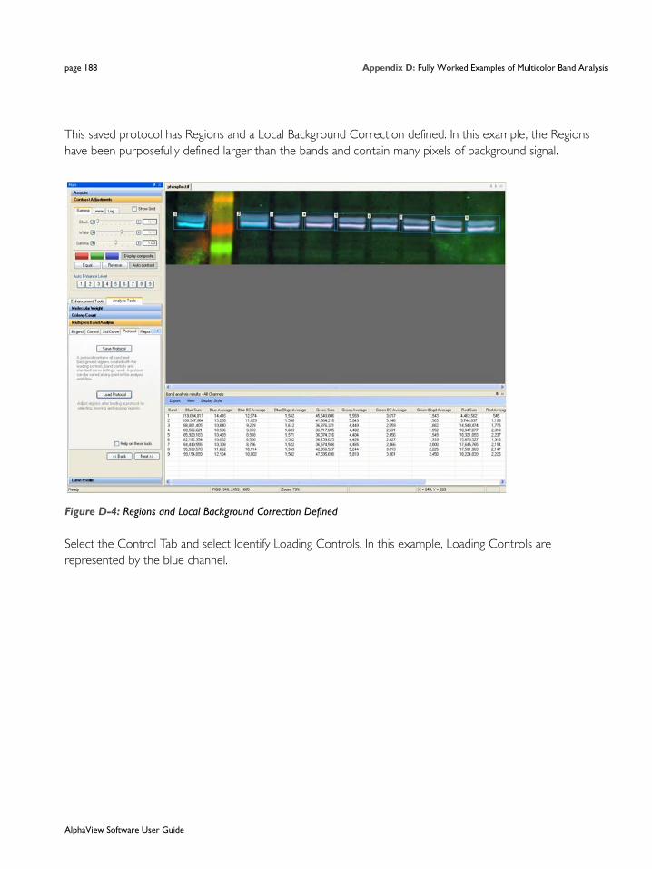
page 188 Appendix D: Fully Worked Examples of Multicolor Band Analysis
This saved protocol has Regions and a Local Background Correction defined. In this example, the Regions have been purposefully defined larger than the bands and contain many pixels of background signal.
Figure D-4: Regions and Local Background Correction Defined
Select the Control Tab and select Identify Loading Controls. In this example, Loading Controls are represented by the blue channel.
AlphaView Software User Guide

Example 1: Phosphorylation page 189
Figure D-5: Identify Loading Controls Select Channel
Select the Blue channel and then select all Regions to identify them as Loading Controls.
AlphaView Software User Guide

page 190 Appendix D: Fully Worked Examples of Multicolor Band Analysis
Figure D-6: Blue Channel Loading Controls
Click the Identify Loading Controls button to de-activate the selection tool. Notice the data columns in the data table show the blue and red values for the background-corrected average (BC Average); Local Background correction was pre-defined for this protocol.
The data table also displays the Loading Control Normalized data (LCN Avg)
NOTE: All Blue LCN Avg values are identical. This is expected, because the Blue channel is designated as the Loading Control, and the calculation for the Loading Control determines the mean intensity for all Loading Controls. In this example the Blue Loading Control values are calculated from the Blue BC Avg, which represents total protein (X+pX) for each lane. Ideally identical quantities of total protein are loaded in each lane, but in reality slight variations in loading usually occur from lane to lane.
NOTE: The Red LCN Avg is calculated: Red BC Avg * Blue LCN Avg/Blue BC Average, using the respective values for the band of interest (e.g. for band #1: Red LCN Avg = 298*9998/12874=231.
The Red LCN Avg values now represent the pX/(X+pX) ratio for each corresponding band.
AlphaView Software User Guide

Example 1: Phosphorylation page 191
In this example it is not necessary to designate separate experimental bands. The defined Control bands function as experimental bands without explicitly being defined as such.
Select Identify Control Band from the Band Control Normalization section and select the red channel of region #1 (primary band of lane 1), which represents the untreated sample.
Figure D-7: Red Channel Region 1Selection
Select Identify Experimental Bands and select regions 2-9. De-activate this tool by pressing Identify Experimental Bands or right-clicking.
NOTE: The data column Fold Change is populated. The Fold Change column represents up/down regula-tion in phosphorylated protein relative to baseline levels of phosphorylation in the reference sample (Lane 1).
The Fold Change value is calculated using the Red LCN Avg values for each band compared to the Red LCN Avg value for the control band (band #1) (e.g. for band #2: Fold Change = Red LCN AvgBand #2 / Red LCN AvgControl Band #1 = 792/231=3.42).
AlphaView Software User Guide

page 192 Appendix D: Fully Worked Examples of Multicolor Band Analysis
Recall that Red LCN Avg = Red BC Avg *Blue LCN Avg/Blue BC Average for each band, and recall that Red BC Avg = pX, Blue BC Avg=(X+pX).
When the value for Fold Change is calculated: Red LCN AvgBand #2/Red LCN AvgBand #1 the following substitution can be made:
Fold Change = pXBand #2*Blue LCN Avg/(X+pX)Band#2 / pXBand #1*Blue LCN Avg/(X+pX)Band#1 and notice the value Blue LCN Avg cancels, leaving the desired result.
Fold ChangeBand#2 = , which is the level of phosphorylation relative to the total amount of protein for band #2 compared to the baseline level of phosphorylation relative to the total amount of protein for Band # (the untreated sample).
Repeat the above for the other bands to complete the analysis.
The data table can be exported and Microsoft Excel utilized to prepare graphs.
Figure D-8: Phosphorylation Response Chart
Example 2: Quantitation Across Color ChannelsIn this example the multicolor blot includes a dilution series in the red channel and a treatment course indicating expression level changes for a phosphorylated isoform in the green channel. There is also a specially constructed control sample that serves as a loading control, as well as a control for color channel normalization (Color Control). In this example, the goal is to determine the absolute concentration of the phosphorylated isoform (green signal) using the dilution series in the red channel as a standard curve.
AlphaView Software User Guide

Example 2: Quantitation Across Color Channels page 193
The Color Control is constructed using equi-molar concentrations of a reference protein that has been separately labeled with the GE DIGE minimal dye labeling kit using CY2, CY3 and CY5 dyes. Therefore, the Color Control has a known quantity of material in all three color channels (in this case the relative ratios are 1:1:1). This Color Control permits direct comparison of the red, green and blue channel data when the corresponding signals are normalized to the Color Control signals; this process is termed Color Control Normalization or CCN.
Following the steps in the above Example #1, launch AlphaView and open the image “Quant.tif ”. Then, open the Multiplex Band Analysis module and load the protocol “quant.sda”.
Figure D-9: Quantitation Across Color Channels
In Figure D-9, bands 1–6 are the Color Control bands serving as loading controls. Any color channel can be used to perform the Loading Control Normalization.
Bands 7–12 of green channel data represent the signal from the phospho-specific antibody, with band 7 being the reference sample not subject to treatment.
Bands 13–18 of red channel data represent the dilution series with the following amounts of protein from left to right 0, 0.4, 1.1, 3.3, 10, and 30 (nanograms).
Select the Background tab and select Local Background.
AlphaView Software User Guide

page 194 Appendix D: Fully Worked Examples of Multicolor Band Analysis
Select the Control Tab and Identify Loading Controls by choosing the blue channel and selecting bands 1–6. De-activate the Loading Control tool by selecting the Identify Loading Controls button (or right mouse click).
Select Identify Experimental Bands and select bands 7–12. The Identify Experimental Bands feature is automatically de-activated if the number of experimental bands matches the number of control bands.
Press the Identify Experimental Bands button again and select bands 13–18.
Figure D-10: Quantitation Loading Control Normalized Values
NOTE: The data table shows the Loading Control Normalized (LCN) values for all bands and all color
channels.
Use the Band Control Normalization tool to determine the Fold Change in the phosphorylated samples relative to Band 7.
Select Identify Control Band in the Band Control Normalization section and select the green channel and Band 7.
Select Identify Experiment Bands, and select bands 8–12. Fold Change values are populated in the data table.
AlphaView Software User Guide

Example 2: Quantitation Across Color Channels page 195
Figure D-11: Band Analysis Results—All Channels
Select the Std Curve tab to construct a quantitative curve. Select Add Items..., and select the red channel. Select bands 13–18. Band 18 has a concentration of 0ng. De-activate the Add Items… tool by selecting Add Items… again.
Figure D-12: Multiplex Band Analysis
AlphaView Software User Guide

page 196 Appendix D: Fully Worked Examples of Multicolor Band Analysis
In the Std Curve data table, enter the known concentrations of protein for each standard. Select an appropriate Curve Fitting model and select an appropriate Y axis parameter (LCN Avg is preferable in this example). Once the known concentrations are entered, the curve fit is calculated and a graph plotted.
Figure D-13: Calculated Curve Fit and Graph
In Figure D-13, the known concentrations appear in the table of the Std Curve section, as well as in the results data table. A new column appears in the results data table displaying the calculated concentrations for the Experimental bands for the red channel. The standard concentrations are highlighted in green and the band number is marked with an “s” for Standard.
To determine the concentrations of phosphorylated protein (the green signal in bands 7–12), use the signals for the Color Control bands to make cross-channel calibrations of the mass standards.
Select Identify CC Band in the Color Control Normalization section and select band 1. In the Amounts section of Color Control Normalization, enter values for Red, Green and Blue. In this example an equi-molar ratio of 1:1:1 is represented.
AlphaView Software User Guide

Example 2: Quantitation Across Color Channels page 197
Figure D-14: Green Channel Phosphorylated Protein (Green ng)
In Figure D-14, the values in the results data table display the nanogram concentrations of phosphorylated protein (represented by the green channel data) in the column labeled Green ng. Hover the mouse pointer over the column Green ng for Band 7, and the tool tip displays the band number and the data value. The value for Band 8 displays a “-“ indicating the concentration is outside the range defined by the known concentrations used from the red channel data to construct the mass standard curve. Only values within the defined range are accurately quantified.
AlphaView Software User Guide

page 198 Appendix D: Fully Worked Examples of Multicolor Band Analysis
AlphaView Software User Guide