alternate direction implicit method for a stochastic … ait...stochastic local volatility model...
TRANSCRIPT
Stochastic Local Volatility ModelAlternate Direction Implicit Scheme: ADI
ResultsConclusion
Alternate Direction Implicit Method for aStochastic Local Volatility Model:
High Performance Computing Platforms Comparison
Zaid AIT HADDOUManchester Business School
May 15, 2013HPCFinance conference
Tampere
1 / 41

Stochastic Local Volatility ModelAlternate Direction Implicit Scheme: ADI
ResultsConclusion
Outline
1 Stochastic Local Volatility ModelWhy a Stochastic Local Volatility Model ?SLV CalibrationLeverage Function CalibrationOption Pricing
2 Alternate Direction Implicit Scheme: ADIWhat is ADI ?Simple Implementation of the ADI SchemeADI for Heston PDETridiagonal Systems Solvers
3 ResultsVolatility & Leverage FunctionCall Options PriceExperimental EnvironmentCUDA ImplementationPlatform Comparison
4 Conclusion
2 / 41
Stochastic Local Volatility ModelAlternate Direction Implicit Scheme: ADI
ResultsConclusion
Why a Stochastic Local Volatility Model ?SLV CalibrationLeverage Function CalibrationOption Pricing
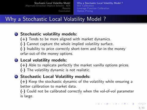
Why a Stochastic Local Volatility Model ?
1 Stochastic volatility models:(+) Tends to be more aligned with market dynamics.(-) Cannot capture the whole implied volatility surface.(-) Inability to price correctly short-term and far-in-the moneyorfar-out-of-the money options.
2 Local volatility models:(+) Able to replicate perfectly the market vanilla options prices.(-) The volatility dynamic is not realistic.
3 Stochastic Local Volatility models:(+) Keep the stochastic dynamic of the volatility while ensuring abetter calibration to market data.(-) Could not be calibrated correctly when the vol-of-vol parameteris large.
3 / 41

Stochastic Local Volatility ModelAlternate Direction Implicit Scheme: ADI
ResultsConclusion
Why a Stochastic Local Volatility Model ?SLV CalibrationLeverage Function CalibrationOption Pricing
Why a Stochastic Local Volatility Model ?
1 SLV model:
SLV is a combination of a Local & Stochastic Volatility model
Implemented SLV
dSt = rStdt + L(St , t)√νtStdW
1t (1)
dνt = k(θ − νt) + ξ√νtdW
2t (2)
dW 1t .dW
2t = ρdt
L(St , t): is the leverage function and it represents theweight of local volatility in the model.
4 / 41
Stochastic Local Volatility ModelAlternate Direction Implicit Scheme: ADI
ResultsConclusion
Why a Stochastic Local Volatility Model ?SLV CalibrationLeverage Function CalibrationOption Pricing
SLV Calibration
Two steps calibration:
1 Find the stochastic parameters of the pure Heston model tomatch given market implied volatility data.
2 Calibrate the leverage function L(St , t) to the local volatilitysurface.
5 / 41
Stochastic Local Volatility ModelAlternate Direction Implicit Scheme: ADI
ResultsConclusion
Why a Stochastic Local Volatility Model ?SLV CalibrationLeverage Function CalibrationOption Pricing
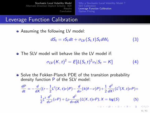
Leverage Function Calibration
Assuming the following LV model:
dSt = rStdt + σLV (St,t)StdWt (3)
The SLV model will behave like the LV model if:
σLV (K , t)2 = E [L(St,t)2νt |St = K ] (4)
Solve the Fokker-Planck PDE of the transition probabilitydensity function P of the SLV model:
dP
dt= − d
dX((r− 1
2L2(X , t)ν)P)− d
dν(k(θ−ν)P)+
1
2
d2
dX 2(L2(X , t)νP)+
1
2ξ2 d2
dν2(νP) + ξρ
d2
dνdX(L(X , t)νP);X = log(S) (5)
6 / 41

Stochastic Local Volatility ModelAlternate Direction Implicit Scheme: ADI
ResultsConclusion
Why a Stochastic Local Volatility Model ?SLV CalibrationLeverage Function CalibrationOption Pricing
Leverage Function Calibration
Figure : Initial probability distribution for the forward Fokker-Planck PDE
7 / 41
Stochastic Local Volatility ModelAlternate Direction Implicit Scheme: ADI
ResultsConclusion
Why a Stochastic Local Volatility Model ?SLV CalibrationLeverage Function CalibrationOption Pricing
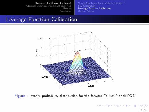
Leverage Function Calibration
Figure : Interim probability distribution for the forward Fokker-Planck PDE
8 / 41
Stochastic Local Volatility ModelAlternate Direction Implicit Scheme: ADI
ResultsConclusion
Why a Stochastic Local Volatility Model ?SLV CalibrationLeverage Function CalibrationOption Pricing
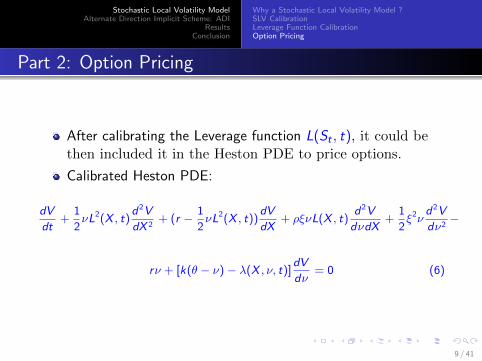
Part 2: Option Pricing
After calibrating the Leverage function L(St , t), it could bethen included it in the Heston PDE to price options.
Calibrated Heston PDE:
dV
dt+
1
2νL2(X , t)
d2V
dX 2+ (r − 1
2νL2(X , t))
dV
dX+ ρξνL(X , t)
d2V
dνdX+
1
2ξ2ν
d2V
dν2−
rν + [k(θ − ν) − λ(X , ν, t)]dV
dν= 0 (6)
9 / 41
Stochastic Local Volatility ModelAlternate Direction Implicit Scheme: ADI
ResultsConclusion
What is ADI ?Simple Implementation of the ADI SchemeADI for Heston PDETridiagonal Systems Solvers
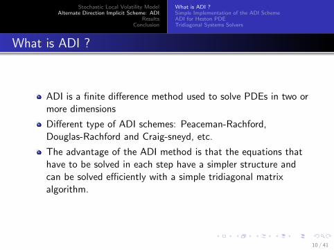
What is ADI ?
ADI is a finite difference method used to solve PDEs in two ormore dimensions
Different type of ADI schemes: Peaceman-Rachford,Douglas-Rachford and Craig-sneyd, etc.
The advantage of the ADI method is that the equations thathave to be solved in each step have a simpler structure andcan be solved efficiently with a simple tridiagonal matrixalgorithm.
10 / 41
Stochastic Local Volatility ModelAlternate Direction Implicit Scheme: ADI
ResultsConclusion
What is ADI ?Simple Implementation of the ADI SchemeADI for Heston PDETridiagonal Systems Solvers
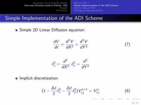
Simple Implementation of the ADI Scheme
Simple 2D Linear Diffusion equation:
dV
dt=
d2V
dX 2+
d2V
dY 2(7)
δ2x =
d2
dX 2; δ2
y =d2
dY 2
Implicit discretization:
(1− ∆t
2δ2x −
∆t
2δ2y )V n+1
i ,j = V ni ,j (8)
11 / 41
Stochastic Local Volatility ModelAlternate Direction Implicit Scheme: ADI
ResultsConclusion
What is ADI ?Simple Implementation of the ADI SchemeADI for Heston PDETridiagonal Systems Solvers
Simple Implementation of the ADI Scheme
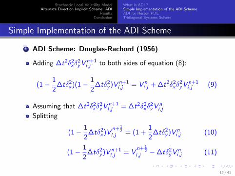
1 ADI Scheme: Douglas-Rachord (1956)
Adding ∆t2δ2xδ
2yV
n+1i ,j to both sides of equation (8):
(1− 1
2∆tδ2
x)(1− 1
2∆tδ2
y )V n+1i ,j = V n
i ,j + ∆t2δ2xδ
2yV
n+1i ,j (9)
Assuming that ∆t2δ2xδ
2yV
n+1i ,j = ∆t2δ2
xδ2yV
ni ,j
Splitting
(1− 1
2∆tδ2
x)Vn+ 1
2i ,j = (1 +
1
2∆tδ2
y )V ni ,j (10)
(1− 1
2∆tδ2
y )V n+1i ,j = V
n+ 12
i ,j −∆tδ2yV
ni ,j (11)
12 / 41

Stochastic Local Volatility ModelAlternate Direction Implicit Scheme: ADI
ResultsConclusion
What is ADI ?Simple Implementation of the ADI SchemeADI for Heston PDETridiagonal Systems Solvers
ADI for Heston PDE
Using Crank Nicolson discretization instead of its implicitcounterpart.
Following the same logic explained in the previous example:
(1− 1
2∆tA1)V
n+ 12
i ,j = (1 + A0 +1
2∆tA1 +
1
2∆tA2)V n
i ,j (12)
(1− 1
2∆tA2)V n+1
i ,j = Vn+ 1
2i ,j − 1
2∆tA2V
ni .j (13)
We deal with the mixed derivative term A0 only explicitly.
13 / 41
Stochastic Local Volatility ModelAlternate Direction Implicit Scheme: ADI
ResultsConclusion
What is ADI ?Simple Implementation of the ADI SchemeADI for Heston PDETridiagonal Systems Solvers
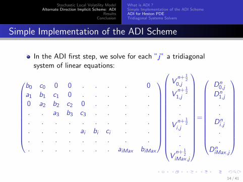
Simple Implementation of the ADI Scheme
In the ADI first step, we solve for each ”j” a tridiagonalsystem of linear equations:
b0 c0 0 0 . . . . 0a1 b1 c1 0 . . . . .0 a2 b2 c2 0 . . . .. . a3 b3 c3 . . . .. . . . . . . . .. . . . ai bi ci . .. . . . . . . . .. . . . . . . aiMax biMax
Vn+ 1
20,j
Vn+ 1
21,j
.
.
Vn+ 1
2i ,j
.
.
Vn+ 1
2iMax ,j
=
Dn0,j
Dn1,j
.
.Dni ,j
.
.DniMax ,j
14 / 41
Stochastic Local Volatility ModelAlternate Direction Implicit Scheme: ADI
ResultsConclusion
What is ADI ?Simple Implementation of the ADI SchemeADI for Heston PDETridiagonal Systems Solvers
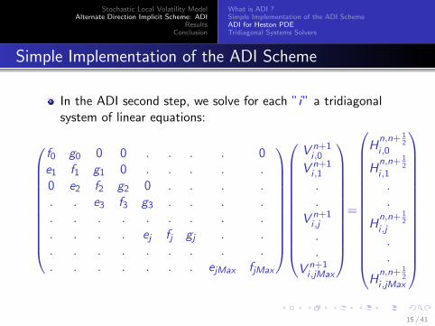
Simple Implementation of the ADI Scheme
In the ADI second step, we solve for each ”i” a tridiagonalsystem of linear equations:
f0 g0 0 0 . . . . 0e1 f1 g1 0 . . . . .0 e2 f2 g2 0 . . . .. . e3 f3 g3 . . . .. . . . . . . . .. . . . ej fj gj . .. . . . . . . . .. . . . . . . ejMax fjMax
V n+1i ,0
V n+1i ,1
.
.
V n+1i ,j
.
.
V n+1i ,jMax
=
Hn,n+ 1
2i ,0
Hn,n+ 1
2i ,1
.
.
Hn,n+ 1
2i ,j
.
.
Hn,n+ 1
2i ,jMax
15 / 41

Stochastic Local Volatility ModelAlternate Direction Implicit Scheme: ADI
ResultsConclusion
What is ADI ?Simple Implementation of the ADI SchemeADI for Heston PDETridiagonal Systems Solvers
Thomas algorithm
1 Thomas algorithm:
Forward elimination:
c′i =
cibi
; i = 1
ci
bi − c′i−1ai
; i = 2, 3, ..., n − 1(14)
d′i =
dibi
; i = 1
di − d′i−1ai
bi − c′i−1ai
; i = 2, 3, ..., n − 1(15)
16 / 41

Stochastic Local Volatility ModelAlternate Direction Implicit Scheme: ADI
ResultsConclusion
What is ADI ?Simple Implementation of the ADI SchemeADI for Heston PDETridiagonal Systems Solvers
Thomas algorithm
1 Thomas algorithm:
Backward substitution:
Vn = d
′n
Vi = d′i − c
′iVi+1
(16)
1 Characteristics:
Complexity O(N).The fastest serial algorithm.
17 / 41
Stochastic Local Volatility ModelAlternate Direction Implicit Scheme: ADI
ResultsConclusion
What is ADI ?Simple Implementation of the ADI SchemeADI for Heston PDETridiagonal Systems Solvers
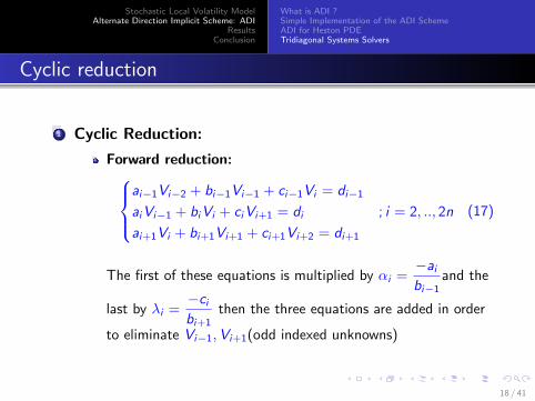
Cyclic reduction
1 Cyclic Reduction:
Forward reduction:ai−1Vi−2 + bi−1Vi−1 + ci−1Vi = di−1
aiVi−1 + biVi + ciVi+1 = di ; i = 2, .., 2n
ai+1Vi + bi+1Vi+1 + ci+1Vi+2 = di+1
(17)
The first of these equations is multiplied by αi =−aibi−1
and the
last by λi =−cibi+1
then the three equations are added in order
to eliminate Vi−1,Vi+1(odd indexed unknowns)
18 / 41

Stochastic Local Volatility ModelAlternate Direction Implicit Scheme: ADI
ResultsConclusion
What is ADI ?Simple Implementation of the ADI SchemeADI for Heston PDETridiagonal Systems Solvers
Cyclic reduction
1 Cyclic Reduction:
Forward reduction:
a(1)i Vi−2 + b
(1)i Vi + c
(1)i Vi+2 = y
(1)i ; i = 2, .., 2n (18)
Backward substitution:We use the even-indexed unknowns found through the forwardreduction in order to solve all odd-indexed unknowns.
2 Characteristics:
Complexity O(N)Each step of the CR algorithm could be parallelized.
19 / 41
Stochastic Local Volatility ModelAlternate Direction Implicit Scheme: ADI
ResultsConclusion
What is ADI ?Simple Implementation of the ADI SchemeADI for Heston PDETridiagonal Systems Solvers
Cyclic reduction
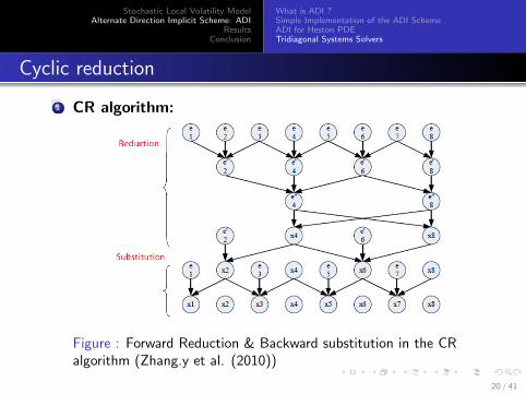
1 CR algorithm:
Figure : Forward Reduction & Backward substitution in the CRalgorithm (Zhang.y et al. (2010))
20 / 41
Stochastic Local Volatility ModelAlternate Direction Implicit Scheme: ADI
ResultsConclusion
What is ADI ?Simple Implementation of the ADI SchemeADI for Heston PDETridiagonal Systems Solvers
Parallel cyclic reduction
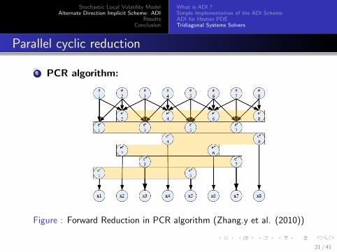
1 PCR algorithm:
Figure : Forward Reduction in PCR algorithm (Zhang.y et al. (2010))
21 / 41

Stochastic Local Volatility ModelAlternate Direction Implicit Scheme: ADI
ResultsConclusion
Volatility & Leverage FunctionCall Options PriceExperimental EnvironmentCUDA ImplementationPlatform Comparison
Market Implied Volatility Surface
Figure : Implied Volatility Surface
22 / 41

Stochastic Local Volatility ModelAlternate Direction Implicit Scheme: ADI
ResultsConclusion
Volatility & Leverage FunctionCall Options PriceExperimental EnvironmentCUDA ImplementationPlatform Comparison
Volatility curves (T=0.5 year)
Figure : Market volatility, Heston implied volatility and Local volatilitycurves for T=0.5
23 / 41

Stochastic Local Volatility ModelAlternate Direction Implicit Scheme: ADI
ResultsConclusion
Volatility & Leverage FunctionCall Options PriceExperimental EnvironmentCUDA ImplementationPlatform Comparison
Leverage function surface
Figure : Leverage function surface
24 / 41

Stochastic Local Volatility ModelAlternate Direction Implicit Scheme: ADI
ResultsConclusion
Volatility & Leverage FunctionCall Options PriceExperimental EnvironmentCUDA ImplementationPlatform Comparison
Call options pricing error
V0 ξ k θ S0 ρ r T
0.0713 0.4 1 0.2 120 0.3874 0.02 0.5
Table : Heston Parameters
Strike LV Heston SLV market price
180 0.0338 0.1532 0.0383 1.0665
100 0.0013 0.1648 0.0183 23.3577
Table : Pricing error according to different models
25 / 41
Stochastic Local Volatility ModelAlternate Direction Implicit Scheme: ADI
ResultsConclusion
Volatility & Leverage FunctionCall Options PriceExperimental EnvironmentCUDA ImplementationPlatform Comparison
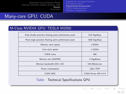
Many-core GPU: CUDA
M-Class NVIDIA GPU: TESLA M2050
Peak double precision floating point performance peak 515 Gigaflops
Peak single precision floating point performance peak 1030 Gigaflops
Memory clock speed 1.55GHz
Core clock speed 1.15GHz
CUDA cores 448
Memory size (GDDR5) 3 GigaBytes
Memory bandwidth (ECC off) 148 GBytes/sec
Power consumption 225w TDP
CUDA SDK CUDA Driver API 4.2.9
Table : Technical Specifications GPU
26 / 41
Stochastic Local Volatility ModelAlternate Direction Implicit Scheme: ADI
ResultsConclusion
Volatility & Leverage FunctionCall Options PriceExperimental EnvironmentCUDA ImplementationPlatform Comparison
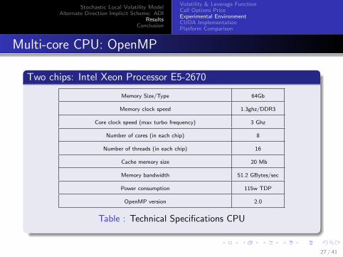
Multi-core CPU: OpenMP
Two chips: Intel Xeon Processor E5-2670
Memory Size/Type 64Gb
Memory clock speed 1.3ghz/DDR3
Core clock speed (max turbo frequency) 3 Ghz
Number of cores (in each chip) 8
Number of threads (in each chip) 16
Cache memory size 20 Mb
Memory bandwidth 51.2 GBytes/sec
Power consumption 115w TDP
OpenMP version 2.0
Table : Technical Specifications CPU
27 / 41

Stochastic Local Volatility ModelAlternate Direction Implicit Scheme: ADI
ResultsConclusion
Volatility & Leverage FunctionCall Options PriceExperimental EnvironmentCUDA ImplementationPlatform Comparison
GPU implementation: Method 1
1 First method on GPU: Thomas-CUDA
All data arrays are stored linearly on the GPU global memory.Two kernels (each kernel solve one ADI step)Each thread build and solve one tridiagonal system usingThomas algorithm.The Transfer of the results from the GPU to the CPU happensonce after completing the time iterations.
2 Charasteristics:
Very easy to implement.Global memory is slow.For 2D ADI most GPU cores are idle.
28 / 41

Stochastic Local Volatility ModelAlternate Direction Implicit Scheme: ADI
ResultsConclusion
Volatility & Leverage FunctionCall Options PriceExperimental EnvironmentCUDA ImplementationPlatform Comparison
GPU implementation: Method 2
1 Second method on GPU: PCR-CUDA
The lower, main and upper diagonals of the tridiagonal systemare all stored linearly in the GPU shared memory.Two kernels (each kernel solve one ADI step)Each tridiagonal system is solved and built by all the blockthreads using the PCR algorithm.The transfer of the results from the GPU to the CPU happensonce after completing the time iterations.
2 Charasteristics:
Harder to implement.Shared memory is fast.For 2D ADI, quite good use of GPU cores.
29 / 41
Stochastic Local Volatility ModelAlternate Direction Implicit Scheme: ADI
ResultsConclusion
Volatility & Leverage FunctionCall Options PriceExperimental EnvironmentCUDA ImplementationPlatform Comparison
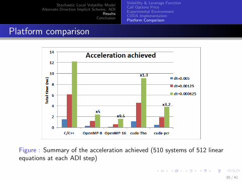
Platform comparison
Figure : Summary of the acceleration achieved (510 systems of 512 linearequations at each ADI step)
30 / 41
Stochastic Local Volatility ModelAlternate Direction Implicit Scheme: ADI
ResultsConclusion
Volatility & Leverage FunctionCall Options PriceExperimental EnvironmentCUDA ImplementationPlatform Comparison
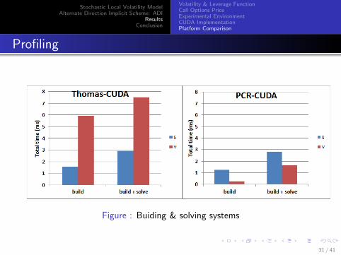
Profiling
Figure : Buiding & solving systems
31 / 41

Stochastic Local Volatility ModelAlternate Direction Implicit Scheme: ADI
ResultsConclusion
Volatility & Leverage FunctionCall Options PriceExperimental EnvironmentCUDA ImplementationPlatform Comparison
Profiling
1 First Method: Thomas-CUDA
Poor performance in the V direction due to uncoalescedglobal memory access.
2 Second method: PCR-CUDA
Poor performance in the S direction due to uncoalescedglobal memory access.
32 / 41

Stochastic Local Volatility ModelAlternate Direction Implicit Scheme: ADI
ResultsConclusion
Volatility & Leverage FunctionCall Options PriceExperimental EnvironmentCUDA ImplementationPlatform Comparison
Global memory access
coalesced global memory access:
Figure : Coalesced memory access
Uncoalesced global memory access:
Figure : Uncoalesced memory access
33 / 41

Stochastic Local Volatility ModelAlternate Direction Implicit Scheme: ADI
ResultsConclusion
Volatility & Leverage FunctionCall Options PriceExperimental EnvironmentCUDA ImplementationPlatform Comparison
Profiling: Memory Optimization
Figure : Building systems optimization
34 / 41
Stochastic Local Volatility ModelAlternate Direction Implicit Scheme: ADI
ResultsConclusion
Volatility & Leverage FunctionCall Options PriceExperimental EnvironmentCUDA ImplementationPlatform Comparison
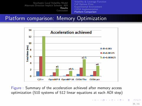
Platform comparison: Memory Optimization
Figure : Summary of the acceleration achieved after memory accessoptimization (510 systems of 512 linear equations at each ADI step)
35 / 41
Stochastic Local Volatility ModelAlternate Direction Implicit Scheme: ADI
ResultsConclusion
Conclusion
SLV models could be a good alternative for SV and LV models.
Calibration is not stable for large vol-of-vol
There are several sources that lead to inaccurate pricing in theSLV model using ADI:
Choice of the boundary conditionsApproximating the leverage function while solving the forwardKolmogorov PDE with ADI.
36 / 41

Stochastic Local Volatility ModelAlternate Direction Implicit Scheme: ADI
ResultsConclusion
Conclusion
Of course ! the GPU codes could still be optimized.
Coalesced global memory access is very important foroptimization.
GPU become much more competitive as we increase thedensity of the grids.
CUDA code requires a reasonable programming effort tooptimize performance !
OpenMP is very easy to implement !
37 / 41
Stochastic Local Volatility ModelAlternate Direction Implicit Scheme: ADI
ResultsConclusion
Questions ?
Thank you for your attention
38 / 41
Stochastic Local Volatility ModelAlternate Direction Implicit Scheme: ADI
ResultsConclusion
References
“Tridiagonal solvers on the GPU and applications to fluid simulation”Nikolai Sakharnykh, GTC 2009
“Fast tridiagonal solvers on the GPU” Y. Zhang, J. Cohen, J.D. Owens,PPoPP 2010
“High performance finite difference PDE solvers on GPUs.” D. Egloff,http://download.quantalea.net/fdm gpu.pdf, Feb. 2010
“Foreign exchange option pricing: A Practitioner’s guide”,IAIN J. Clark,Wiley finance. 2010
“Calibrating and Pricing with Stochastic-Local Volatility Model” Tian. Y,Z. Zili, K. Fima, H. Kais
“On the Numerical solution of heat conduction problems in two and threespace variables”,J. Douglas, JR., H. H. Rachford, JR.
39 / 41

Stochastic Local Volatility ModelAlternate Direction Implicit Scheme: ADI
ResultsConclusion
Acknowledgement
Zaid ait Haddou is a Marie Curie fellow at the University ofManchester. The research leading to these results has receivedfunding from the European Community’s Seventh FrameworkProgramme FP7-PEOPLE-ITN-2008 under grant agreement numberPITN-GA-2009-237984.I would like to thank NAG, advice and technical support, and ChrisArmstrong and Jacques Du Toit (both from NAG) for povidingcodes and for many helpful comments and suggestions.My deepest gratitude goes also to my supervisor Prof. Ser-HuangPoon, in Manchester Business School, for her precious help andunderstanding during the whole project.Furthermore, I would like to acknowledge with much appreciationthe help provided by Mr. Erik Vynkier and also for having me onemonth in SWIP office in Edinburgh.I would like to also thank Mr. Daniel egloff for his technical helpand for providing the PCR solver CUDA code.
40 / 41

Stochastic Local Volatility ModelAlternate Direction Implicit Scheme: ADI
ResultsConclusion
Appendix
ADI for Heston PDE:
A0 corresponds to the mixed derivative term, A1 the spatialderivatives in S direction and A2 the spatial derivatives in Vdirection.
A0 =1
2∆tρσVjSiδsv (19)
A1 =1
2∆t[VjS
2i δss + rSδs − r ] (20)
A2 =1
2∆t[σVjδvv + [k(θ − Vj)− λ(Si ,Vj , t)]δv − r ] (21)
41 / 41