alternating direction algorithms for -problems
TRANSCRIPT

ALTERNATING DIRECTION ALGORITHMS FOR `1-PROBLEMS
IN COMPRESSIVE SENSING
JUNFENG YANG∗ AND YIN ZHANG †
CAAM TR09-37 (REVISED JUNE 6, 2010)
Abstract. In this paper, we propose and study the use of alternating direction algorithms for several `1-norm minimization
problems arising from sparse solution recovery in compressive sensing, including the basis pursuit problem, the basis-pursuit
denoising problems of both unconstrained and constrained forms, as well as others. We present and investigate two classes of
algorithms derived from either the primal or the dual form of `1-problems. The construction of the algorithms consists of two
main steps: (1) to reformulate an `1-problem into one having blockwise separable objective functions by adding new variables
and constraints; and (2) to apply an exact or inexact alternating direction method to the augmented Lagrangian function of the
resulting problem. The derived alternating direction algorithms can be regarded as first-order primal-dual algorithms because
both primal and dual variables are updated at every iteration. Convergence properties of these algorithms are established or
restated when they already exist. Extensive numerical experiments are performed, using randomized partial Walsh-Hadamard
sensing matrices, to demonstrate the versatility and effectiveness of the proposed approach. Moreover, we present numerical
results to emphasize two practically important but perhaps overlooked points: (i) that algorithm speed should be evaluated
relative to appropriate solution accuracy; and (ii) that when erroneous measurements possibly exist, the `1-fidelity should
generally be preferable to the `2-one.
Key words. Compressive sensing, `1-minimization, primal, dual, augmented Lagrangian function, alternating direction
method
AMS subject classifications. 65F22, 65J22, 65K10, 90C25, 90C06
1. Introduction. In the last few years, algorithms for finding sparse solutions of underdetermined
linear systems have been intensively studied, largely because solving such problems constitutes a critical
step in an emerging methodology in digital signal processing — compressive sensing or sampling (CS). In
CS, a digital signal is encoded as inner products between the signal and a set of random (or random-like)
vectors where the number of such inner products, or linear measurements, can be significantly fewer than the
length of the signal. On the other hand, the decoding process requires finding a sparse solution, either exact
or approximate, to an underdetermined linear system. What makes such a scheme work is sparsity; i.e., the
original signal must have a sparse or compressible representation under some known basis. Throughout this
paper we will allow all involved quantities (signals, acquired data and encoding matrices) to be complex.
Let x ∈ Cn be an original signal that we wish to capture. Without loss of generality, we assume that x is
sparse under the canonical basis, i.e., the number of nonzero components in x, denoted by ‖x‖0, is far fewer
than its length. Instead of sampling x directly, in CS one first obtains a set of linear measurements
b = Ax ∈ Cm, (1.1)
where A ∈ Cm×n (m < n) is an encoding matrix. The original signal x is then reconstructed from the
underdetermined linear system Ax = b via certain reconstruction technique. Basic CS theory presented in
[9, 11, 17] states that it is extremely probable to reconstruct x accurately or even exactly from b provided
that x is sufficiently sparse (or compressible) relative to the number of measurements, and the encoding
matrix A possesses certain desirable attributes.
∗Department of Mathematics, Nanjing University, 22 Hankou Road, Nanjing, 210093, P.R. China ([email protected]).†Department of Computational and Applied Mathematics, Rice University, 6100 Main Street, MS-134, Houston, Texas,
77005, U.S.A. ([email protected]).
1
2 J.-F. Yang and Y. Zhang
In the rest of this section, we briefly review the essential ingredients of the CS decoding process and
some existing methods for the relevant optimization problems, summarize our main contributions in this
paper, and describe the notation and organization of the paper.
1.1. Signal Decoding in CS. To make CS successful, two ingredients must be addressed carefully.
First, a sensing matrix A must be designed so that the compressed measurement b = Ax contains enough
information for a successful recovery of x. Second, an efficient, stable and robust reconstruction algorithm
must be available for recovering x from A and b. In the present paper, we will only concentrate on the second
aspect.
In order to recover the sparse signal x from the underdetermined system (1.1), one could naturally
consider seeking among all solutions of (1.1) the sparsest one, i.e., solving
minx∈Cn‖x‖0 : Ax = b, (1.2)
where ‖x‖0 is the number of nonzeros in x. Indeed, with overwhelming probability decoder (1.2) can recover
sparse signals exactly from a very limited number of random measurements (see e.g., [3]). Unfortunately,
this `0-problem is combinatorial and generally computationally intractable. A fundamental decoding model
in CS is the so-called basis pursuit (BP) problem [14]:
minx∈Cn‖x‖1 : Ax = b. (1.3)
Minimizing the `1-norm in (1.3) plays a central role in promoting solution sparsity. In fact, problem (1.3)
shares common solutions with (1.2) under some favorable conditions (see, for example, [18]). When b contains
noise, or when x is not exactly sparse but only compressible, as are the cases in most practical applications,
certain relaxation to the equality constraint in (1.3) is desirable. In such situations, common relaxations to
(1.3) include the constrained basis pursuit denoising (BPδ) problem [14]:
minx∈Cn‖x‖1 : ‖Ax− b‖2 ≤ δ, (1.4)
and its variants including the unconstrained basis pursuit denoising (QPµ) problem
minx∈Cn
‖x‖1 +1
2µ‖Ax− b‖22, (1.5)
where δ, µ > 0 are parameters. From optimization theory, it is well known that problems (1.4) and (1.5) are
equivalent in the sense that solving one will determine a parameter value in the other so that the two share
the same solution. As δ and µ approach zero, both BPδ and QPµ converge to (1.3). In this paper, we also
consider the use of an `1/`1 model of the form
minx∈Cn
‖x‖1 +1
ν‖Ax− b‖1, (1.6)
whenever b might contain erroneous measurements. It is well known that unlike (1.5) where squared `2-norm
fidelity is used, the `1-norm fidelity term makes (1.6) an exact penalty method in the sense that it reduces
to (1.3) when ν > 0 is less than some threshold.
It is worth noting that problems (1.3), (1.4), (1.5) and (1.6) all have their “nonnegative counterparts”
where the signal x is real and nonnegative. These nonnegative counterparts will be briefly considered later.
Finally, we mention that aside from `1-related decoders, there exist alternative decoding techniques such as
greedy algorithms (e.g., [51]) which, however, are not a subject of concern in this paper.

Alternating Direction Algorithms for `1-Problems in Compressive Sensing 3
1.2. Some existing methods. In the last few years, numerous algorithms have been proposed and
studied for solving the aforementioned `1-problems arising in CS. Although these problems are convex pro-
grams with relatively simple structures (e.g., the basis pursuit problem is a linear program when x is real),
they do demand dedicated algorithms because standard methods, such as interior-point algorithms for linear
and quadratic programming, are simply too inefficient on them. This is the consequence of several factors,
most prominently the fact that the data matrix A is totally dense while the solution is sparse. Clearly,
the existing standard algorithms were not designed to handle such a feature. Another noteworthy structure
is that encoding matrices in CS are often formed by randomly taking a subset of rows from orthonormal
transform matrices, such as DCT (discrete cosine transform), DFT (discrete Fourier transform) or DWHT
(discrete Walsh-Hadamard transform) matrices. Such encoding matrices do not require storage and enable
fast matrix-vector multiplications. As a result, first-order algorithms that are able to take advantage of such
a special feature lead to better performance and are highly desirable. In this paper we derive algorithms
that take advantage of the structure (AA∗ = I), and our numerical experiments are focused on randomized
partial transform sensing matrices.
One of the earliest first-order methods applied to solving (1.5) is the gradient projection method sug-
gested in [24] by Figueiredo, Nowak and Wright, where the authors reformulated (1.5) as a box-constrained
quadratic program and implemented a gradient projection method with line search. To date, the most widely
studied class of first-order methods for solving (1.5) is variants of the iterative shrinkage/thresholding (IST)
method, which was first proposed for wavelet-based image deconvolution (see [40, 16, 23], for example) and
then independently discovered and analyzed by many others (for example [21, 47, 48, 15]). In [32] and [33],
Hale, Yin and Zhang derived the IST algorithm from an operator splitting framework and combined it with
a continuation strategy. The resulting algorithm, which is named fixed-point continuation (FPC), is also
accelerated via a non-monotone line search with Barzilai-Borwein steplength [4]. A similar sparse reconstruc-
tion algorithm called SpaRSA was also studied by Wright, Nowak and Figueiredo in [56]. Recently, Beck
and Teboulle proposed a fast IST algorithm (FISTA) in [5], which attains the same optimal convergence in
function values as Nesterov’s multi-step gradient method [39] for minimizing composite convex functions.
Lately, Yun and Toh also studied a block coordinate gradient descent (CGD) method in [61] for solving (1.5).
There exist also algorithms for solving constrained `1-problems (1.3) and (1.4). Bregman iterations,
proposed in [41] and now known to be equivalent to the augmented Lagrangian method, were applied to
the basis pursuit problem by Yin, Osher, Goldfarb and Darbon in [58]. In the same paper, a linearized
Bregman method was also suggested and analyzed subsequently in [7, 8, 59]. In [25], Friedlander and Van
den Berg proposed a spectral projection gradient method (SPGL1), where (1.4) is solved by a root-finding
framework applied to a sequence of LASSO problems [50]. Moreover, based on a smoothing technique studied
by Nesterov in [38], a first-order algorithm called NESTA was proposed by Becker, Bobin and Candes in [6]
for solving (1.4).
1.3. Contributions. After years of intensive research on `1-problem solving, it would appear that most
relevant algorithmic ideas have been either tried or, in many cases, re-discovered. Yet interestingly, until
very recently the classic idea of alternating direction method (ADM) had not, to the best of our knowledge,
been seriously investigated.
The main contributions of this paper are to introduce the ADM approach to the area of solving `1-
problems in CS (as well as solving similar problems in image and signal processing), and to demonstrate
its usefulness as a versatile and powerful algorithmic approach. From the ADM framework we have derived
first-order primal-dual algorithms for models (1.3)-(1.6) and their nonnegative counterparts where signals

4 J.-F. Yang and Y. Zhang
are real and nonnegative. For each model, an ADM algorithm can be derived based on either the primal
or the dual. Since the dual-based algorithms appear to be slightly more efficient when sensing matrices
are orthonormal, we have implemented them in a Matlab package called YALL1 (short for Your ALgorithm
for L1). Currently, YALL1 [62] can effectively solve eight different `1-problems: models (1.3)-(1.6) and their
nonnegative counterparts, where signals can be real (and possibly nonnegative) or complex, and orthonormal
sparsifying bases and weights are also permitted in the `1-regularization term which takes the more general
form ‖Wx‖w,1 ,∑ni=1 wi|(Wx)i| for any W ∈ Cn×n with W ∗W = I and w ∈ Rn with w ≥ 0.
In this paper, we present extensive computational results to document the numerical performance of the
proposed ADM algorithms in comparison to several state-of-the-art algorithms for solving `1-problems under
various situations, including FPC, SpaRSA, FISTA and CGD for solving (1.5), and SPGL1 and NESTA for
solving (1.3) and (1.4). As by-products, we also address a couple of related issues of practical importance;
i.e., choices of optimization models and proper evaluation of algorithm speed.
1.4. Notation. We let ‖ · ‖ be the `2-norm and PΩ(·) be the orthogonal projection operator onto a
closed convex set Ω under the `2-norm. Superscripts “>” and “∗” denote, respectively, the transpose and
the conjugate transpose operators for real and complex quantities. We let Re(·) and | · | be, respectively, the
real part and the magnitude of a complex quantity, which are applied component-wise to complex vectors.
Further notation will be introduced wherever it occurs.
1.5. Organization. This paper is organized as follows. In Section 2, we first review the basic idea of
the classic ADM framework and then derive alternating direction algorithms for solving (1.3), (1.4) and (1.5).
We also establish convergence of the primal-based algorithms, while that of the dual-based algorithms follows
from classic results in the literature when sensing matrices have orthonormal rows. In Section 3, we illustrate
how to reduce model (1.6) to (1.3) and present numerical results to compare the behavior of model (1.6)
to that of models (1.4) and (1.5) under various scenarios of data noise. In Section 4, we first re-emphasize
the sometimes overlooked common sense on appropriate evaluations of algorithm speed, and then present
extensive numerical results on the performance of the proposed ADM algorithms in comparison to several
state-of-the-art algorithms. Finally, we conclude the paper in Section 5 and discuss several extensions of the
ADM approach to other `1-like problems.
2. ADM-based first-order primal-dual algorithms. In this section, based on the classic ADM
technique, we propose first-order primal-dual algorithms that update both primal and dual variables at each
iteration for the solution of `1-problems. We start with a brief review on a general framework of ADM.
2.1. General framework of ADM. Let f(x) : Rm → R and g(y) : Rn → R be convex functions,
A ∈ Rp×m, B ∈ Rp×n and b ∈ Rp. We consider the structured convex optimization problem
minx,yf(x) + g(y) : Ax+By = b , (2.1)
where the variables x and y appear separately in the objective, and are coupled only in the constraint. The
augmented Lagrangian function of this problem is given by
LA(x, y, λ) = f(x) + g(y)− λ>(Ax+By − b) +β
2‖Ax+By − b‖2, (2.2)
where λ ∈ Rp is a Lagrangian multiplier and β > 0 is a penalty parameter. The classic augmented Lagrangian
method [36, 43] iterates as follows: given λk ∈ Rp,(xk+1, yk+1)← arg minx,y LA(x, y, λk),
λk+1 ← λk − γβ(Axk+1 +Byk+1 − b),(2.3)
Alternating Direction Algorithms for `1-Problems in Compressive Sensing 5
where γ ∈ (0, 2) guarantees convergence, as long as the subproblem is solved to an increasingly high accuracy
at every iteration [45]. However, an accurate, joint minimization with respect to both x and y can become
costly. In contrast, ADM utilizes the separability structure in (2.1) and replaces the joint minimization by
two simpler subproblems. Specifically, ADM minimizes LA(x, y, λ) with respect to x and y separately via a
Gauss-Seidel type iteration. After just one sweep of alternating minimization with respect to x and y, the
multiplier λ is updated immediately. In short, given (yk, λk), ADM iterates as followsxk+1 ← arg minx LA(x, yk, λk),
yk+1 ← arg miny LA(xk+1, y, λk),
λk+1 ← λk − γβ(Axk+1 +Byk+1 − b).(2.4)
In the above, the domains for the variables x and y are assumed to be Rm and Rn, respectively, but the
derivation will be the same if these domains are replaced by closed convex sets X ⊂ Rm and Y ⊂ Rn,
respectively. In that case, the minimization problems in (2.4) will be over the sets X and Y , respectively.
The basic idea of ADM goes back to the work of Glowinski and Marocco [30] and Gabay and Mercier
[27]. Let θ1(·) and θ2(·) be convex functionals, and A be a continuous linear operator. The authors of [27]
considered minimizing an energy function of the form
minuθ1(u) + θ2(Au).
By introducing an auxiliary variable v, the above problem was equivalently transformed to
minu,vθ1(u) + θ2(v) : Au− v = 0 ,
which has the form of (2.1) and to which the ADM approach was applied. Subsequently, ADM was studied
extensively in optimization and variational analysis. In [29], ADM is interpreted as the Douglas-Rachford
splitting method [19] applied to a dual problem. The equivalence between ADM and a proximal point method
is shown in [20]. The works applying ADM to convex programming and variational inequalities include
[52, 26, 35], to mention just a few. Moreover, ADM has been extended to allowing inexact minimization (see
[20, 34], for example).
In (2.4), a steplength γ > 0 is attached to the update of λ. Under certain technical assumptions,
convergence of ADM with a steplength γ ∈ (0, (√
5 + 1)/2) was established in [28, 29] in the context
of variational inequality. The shrinkage in the permitted range from (0, 2) in the augmented Lagrangian
method to (0, (√
5 + 1)/2) in ADM is related to relaxing the exact minimization of LA(x, y, λk) with respect
to (x, y) to merely one round of alternating minimization.
Interestingly, the ADM approach was not widely utilized in the field of image and signal processing
(including compressive sensing) until very recently when a burst of works applying ADM techniques appeared
in 2009, including our ADM-based `1-solver package YALL1 ([62], published online in April 2009) and a
number of ADM-related papers (see [22, 57, 31, 42, 1, 2], for example). The rest of the paper is to present
the derivation and performance of the proposed ADM algorithms for solving the `1-models (1.3)-(1.6) and
their nonnegative counterparts, many of which have been implemented in YALL1.
2.2. Applying ADM to primal problems. In this subsection, we apply ADM to primal `1-problems
(1.4) and (1.5). First, we introduce auxiliary variables to reformulate these problems into the form of (2.1).
Then, we apply alternating minimization to the corresponding augmented Lagrangian functions, either
exactly or approximately, to obtain ADM-like algorithms.

6 J.-F. Yang and Y. Zhang
With an auxiliary variable r ∈ Cm, problem (1.5) is clearly equivalent to
minx∈Cn, r∈Cm
‖x‖1 +
1
2µ‖r‖2 : Ax+ r = b
, (2.5)
that has an augmented Lagrangian subproblem of the form
minx∈Cn, r∈Cm
‖x‖1 +
1
2µ‖r‖2 −Re(y∗(Ax+ r − b)) +
β
2‖Ax+ r − b‖2
, (2.6)
where y ∈ Cm is a multiplier and β > 0 is a penalty parameter. Given (xk, yk), we obtain (rk+1, xk+1, yk+1)
by applying alternating minimization to (2.6). First, it is easy to show that, for x = xk and y = yk fixed,
the minimizer of (2.6) with respect to r is given by
rk+1 =µβ
1 + µβ
(yk/β − (Axk − b)
). (2.7)
Second, for r = rk+1 and y = yk fixed, simple manipulation shows that the minimization of (2.6) with
respect to x is equivalent to
minx∈Cn
‖x‖1 +β
2‖Ax+ rk+1 − b− yk/β‖2, (2.8)
which itself is in the form of (1.5). However, instead of solving (2.8) exactly, we approximate it by
minx∈Cn
‖x‖1 + β
(Re((gk)∗(x− xk)) +
1
2τ‖x− xk‖2
), (2.9)
where τ > 0 is a proximal parameter and
gk , A∗(Axk + rk+1 − b− yk/β) (2.10)
is the gradient of the quadratic term in (2.8) at x = xk excluding the multiplication by β. The solution of
(2.9) is given explicitly by (see e.g., [15, 32])
xk+1 = Shrink
(xk − τgk, τ
β
), max
|xk − τgk| − τ
β, 0
xk − τgk
|xk − τgk|, (2.11)
where all the operations are performed component-wise and 0 ∗ 00 = 0 is assumed. When the quantities in-
volved are all real, the set of component-wise operation defined in (2.11) is well-known as the one-dimensional
shrinkage (or soft thresholding). Finally, we update the multiplier y by
yk+1 = yk − γβ(Axk+1 + rk+1 − b), (2.12)
where γ > 0 is a constant. In short, ADM applied to (1.5) produces the iteration:rk+1 = µβ
1+µβ
(yk/β − (Axk − b)
),
xk+1 = Shrink(xk − τgk, τβ
),
yk+1 = yk − γβ(Axk+1 + rk+1 − b).
(2.13)
We note that (2.13) is an inexact ADM because the x-subproblem is solved approximately. The convergence
of (2.13) is not covered by the analysis given in [20] where each ADM subproblem is required to be solved
more and more accurately as the algorithm proceeds. On the other hand, the analysis in [34] does cover the

Alternating Direction Algorithms for `1-Problems in Compressive Sensing 7
convergence of (2.13) but only for the case γ = 1. A more general convergence result for (2.13) is established
below that allows γ > 1.
Theorem 2.1. Let τ, γ > 0 satisfy τλmax + γ < 2, where λmax denotes the maximum eigenvalue of
A∗A. For any fixed β > 0, the sequence (rk, xk, yk) generated by (2.13) from any starting point (x0, y0)
converges to (r, x, y), where (r, x) is a solution of (2.5).
Proof. The proof is given in Appendix A.
A similar alternating minimization idea can also be applied to problem (1.4), which is equivalent to
minx∈Cn, r∈Cm
‖x‖1 : Ax+ r = b, ‖r‖ ≤ δ , (2.14)
and has an augmented Lagrangian subproblem of the form
minx∈Cn, r∈Cm
‖x‖1 −Re(y∗(Ax+ r − b)) +
β
2‖Ax+ r − b‖2 : ‖r‖ ≤ δ
. (2.15)
Similar to the derivation of (2.13), applying inexact alternating minimization to (2.15) yields the following
iteration scheme: rk+1 = PBδ
(yk/β − (Axk − b)
),
xk+1 = Shrink(xk − τgk, τ/β),
yk+1 = yk − γβ(Axk+1 + rk+1 − b),(2.16)
where gk is defined as in (2.10), and PBδ is the orthogonal projection (in Euclidean norm) onto the set
Bδ , ξ ∈ Cm : ‖ξ‖ ≤ δ. This algorithm also has a similar convergence result as (2.13).
Theorem 2.2. Let τ, γ > 0 satisfy τλmax + γ < 2, where λmax denotes the maximum eigenvalue of
A∗A. For any fixed β > 0, the sequence (rk, xk, yk) generated by (2.16) from any starting point (x0, y0)
converges to (r, x, y), where (r, x) solves (2.14).
The proof of Theorem 2.2 is similar to that of Theorem 2.1, and thus is omitted.
We point out that, when µ = δ = 0, both (2.13) and (2.16) reduce toxk+1 = Shrink
(xk − τA∗(Axk − b− yk/β), τ/β
),
yk+1 = yk − γβ(Axk+1 − b).(2.17)
It is easy to show that xk+1 given in (2.17) is a solution of
minx‖x‖1 −Re((yk)∗(Ax− b)) +
β
2τ‖x− (xk − τA∗(Axk − b))‖2, (2.18)
which approximates at xk the augmented Lagrangian subproblem of (1.3):
minx‖x‖1 −Re((yk)∗(Ax− b)) +
β
2‖Ax− b‖2
by linearizing 12‖Ax−b‖
2 and adding a proximal term. Therefore, (2.17) is an inexact augmented Lagrangian
algorithm for the basis pursuit problem (1.3). The only difference between (2.17) and the linearized Bregman
method proposed in [58] lies in the updating of the multiplier. The advantage of (2.17) is that it solves (1.3),
while the linearized Bregman method solves a penalty approximation of (1.3), see e.g., [59]. We have the
following convergence result for the iteration scheme (2.17).
Theorem 2.3. Let τ, γ > 0 satisfy τλmax +γ < 2, where λmax denotes the maximum eigenvalue of A∗A.
For any fixed β > 0, the sequence (xk, yk) generated by (2.17) from any starting point (x0, y0) converges
to (x, y), where x is a solution of (1.3).

8 J.-F. Yang and Y. Zhang
Proof. A sketch of proof of this theorem is given in Appendix B.
Since we applied the ADM idea to the primal problems (1.3), (1.4) and (1.5), we name the resulting
algorithms (2.13), (2.16) and (2.17) primal-based ADMs or PADMs in short. In fact, these algorithms are
really of primal-dual nature because both the primal and the dual variables are updated at each and every
iteration. In addition, these are obviously first-order algorithms.
2.3. Applying ADM to dual problems. Similarly, we can apply the ADM idea to the dual problems
of (1.4) and (1.5), resulting in equally simple yet more efficient algorithms when the sensing matrix A
has orthonormal rows. Throughout this subsection, we will make the assumption that the rows of A are
orthonormal, i.e., AA∗ = I. At the end of this section, we will extend the derived algorithms to matrices
with non-orthonormal rows.
Simple computation shows that the dual of (1.5) or equivalently (2.5) is given by
maxy∈Cm
minx∈Cn,r∈Cm
‖x‖1 +
1
2µ‖r‖2 −Re(y∗(Ax+ r − b))
= maxy∈Cm
Re(b∗y)− µ
2‖y‖2 + min
x∈Cn(‖x‖1 −Re(y∗Ax)) +
1
2µminr∈Cm
‖r − µy‖2
= maxy∈Cm
Re(b∗y)− µ
2‖y‖2 : A∗y ∈ B∞1
, (2.19)
where B∞1 , ξ ∈ Cn : ‖ξ‖∞ ≤ 1. By introducing z ∈ Cn, (2.19) is equivalently transformed to
maxy∈Cm
fd(y) , Re(b∗y)− µ
2‖y‖2 : z −A∗y = 0, z ∈ B∞1
, (2.20)
which has an augmented Lagrangian subproblem of the form
miny∈Cm,z∈Cn
−Re(b∗y) +
µ
2‖y‖2 −Re(x∗(z −A∗y)) +
β
2‖z −A∗y‖2, z ∈ B∞1
, (2.21)
where x ∈ Cn is a multiplier (in fact, the primal variable) and β > 0 is a penalty parameter. Now we apply
the ADM scheme to (2.20). First, it is easy to show that, for x = xk and y = yk fixed, the minimizer zk+1
of (2.21) with respect to z is given explicitly by
zk+1 = PB∞1(A∗yk + xk/β), (2.22)
where, as in the rest of the paper, P represent an orthogonal projection (in Euclidean norm) onto a closed
convex set denoted by the subscript. Second, for x = xk and z = zk+1 fixed, the minimization of (2.21) with
respect to y is a least squares problem and the corresponding normal equations are
(µI + βAA∗)y = βAzk+1 − (Axk − b). (2.23)
Under the assumption AA∗ = I, the solution yk+1 of (2.23) is given by
yk+1 =β
µ+ β
(Azk+1 − (Axk − b)/β
). (2.24)
Finally, we update x as follows
xk+1 = xk − γβ(zk+1 −A∗yk+1), (2.25)
where γ ∈ (0, (√
5 + 1)/2). Thus, the ADM scheme for (2.20) is as follows:zk+1 = PB∞1
(A∗yk + xk/β),
yk+1 = βµ+β
(Azk+1 − (Axk − b)/β
),
xk+1 = xk − γβ(zk+1 −A∗yk+1).
(2.26)
Alternating Direction Algorithms for `1-Problems in Compressive Sensing 9
Similarly, the ADM technique can also be applied to the dual of (1.4) given by
maxy∈Cm
b∗y − δ‖y‖ : A∗y ∈ B∞1 , (2.27)
and produces the iteration schemezk+1 = PB∞1
(A∗yk + xk/β),
yk+1 = S(Azk+1 − (Axk − b)/β, δ/β
),
xk+1 = xk − γβ(zk+1 −A∗yk+1),
(2.28)
where S(v, δ/β) , v − PBδ/β (v) with Bδ/β being the Euclidian ball in Cm with radius δ/β.
Under the assumption AA∗ = I, (2.26) is an exact ADM in the sense that each subproblem is solved
exactly. From convergence results in [28, 29], for any β > 0 and γ ∈ (0, (√
5+1)/2), the sequence (xk, yk, zk)generated by (2.26) from any starting point (x0, y0) converges to (x, y, z), which solves the primal-dual pair
(1.5) and (2.20). Similar arguments apply to (2.28) and the primal-dual pair (1.4) and (2.27).
Derived from the dual problems, we name the algorithms (2.26) and (2.28) dual-based ADMs or simply
DADMs. Again we note these are in fact first-order primal-dual algorithms.
It is easy to show that the dual of (1.3) is given by
maxy∈Cm
Re(b∗y) : A∗y ∈ B∞1 , (2.29)
which is a special case of (2.19) and (2.27) with µ = δ = 0. Therefore, both (2.26) and (2.28) can be applied
to solve (1.3). Specifically, when µ = δ = 0, both (2.26) and (2.28) reduce tozk+1 = PB∞1
(A∗yk + xk/β),
yk+1 = Azk+1 − (Axk − b)/β,xk+1 = xk − γβ(zk+1 −A∗yk+1).
(2.30)
We note that the last equality in (2.19) holds if and only if r = µy. Therefore, the primal-dual residues
and the duality gap between (2.5) and (2.20) can be defined byrp , Ax+ r − b ≡ Ax+ µy − b,rd , A∗y − z,∆ , fd(y)− fp(x, r) ≡ Re(b∗y)− µ‖y‖2 − ‖x‖1.
(2.31)
In computation, algorithm (2.26) can be terminated by
Res , max‖rp‖/‖b‖, ‖rd‖/
√m, ∆/fp(x, r)
≤ ε (2.32)
where ε > 0 is a stopping tolerance for the relative optimality residue.
When AA∗ 6= I, the solution of (2.23) could be costly. In this case, we take a steepest descent step in
the y direction and obtain the following iteration scheme:zk+1 = PB∞1
(A∗yk + xk/β),
yk+1 = yk − α∗kgk,xk+1 = xk − γβ(zk+1 −A∗yk+1),
(2.33)
where gk and α∗k are given by
gk = µyk +Axk − b+ βA(A∗yk − zk+1) and α∗k =(gk)∗gk
(gk)∗ (µI + βAA∗) gk. (2.34)
10 J.-F. Yang and Y. Zhang
In our experiments, algorithm (2.33) converges very well for random matrices where AA∗ 6= I, although its
convergence remains an issue of further research. Similar arguments apply to (2.27).
The ADM idea can also be easily applied to `1-problems for recovering real and nonnegative signals. As
an example, we consider model (1.5) plus nonnegativity constraints:
minx∈Rn
‖x‖1 +
1
2µ‖Ax− b‖2 : x ≥ 0
, (2.35)
where (A, b) can remain complex, e.g., A being a partial Fourier matrix. A similar derivation as for (2.19)
shows that a dual problem of (2.35) is equivalent to
maxy∈Cm
Re(b∗y)− µ
2‖y‖2 : z −A∗y = 0, z ∈ F
, (2.36)
where F , z ∈ Cn : Re(z) ≤ 1. The only difference between (2.36) and (2.20) lies in the changing of
constraints on z from z ∈ B∞1 to z ∈ F . Applying the ADM idea to (2.36) yields an iterative algorithm with
the same updating formulae as (2.26) except the computation for zk+1 is replaced by
zk+1 = PF (A∗yk + xk/β). (2.37)
It is clear that the projection onto F is trivial. The same procedure applies to the dual problems of other
`1-problems with nonnegativity constraints as well. Currently, with simple optional parameter settings, our
Matlab package YALL1 [62] can be applied to models (1.3)-(1.6) and their nonnegative counterparts.
3. Choice of denoising models. In this section, we make a digression to emphasize an important
issue in choosing denoising models in CS. In practical applications, measured data are usually contaminated
by noise of different kinds or combinations. To date, the most widely used denoising models in CS are (1.4)
and its variants that use the `2-fidelity, implicitly assuming that the noise is Gaussian. In this section, we
aim to demonstrate that the model (1.6) with `1-fidelity is capable of handing several noise scenarios.
First, it is easy to observe that (1.6) can be reformulated into the form of the basis pursuit model (1.3).
Clearly, (1.6) is equivalent to minx,r ν‖x‖1 + ‖r‖1 : Ax+ r = b, which can be rewritten into
minx‖x‖1 : Ax = b, where A =
[A νI]√1 + ν2
, b =νb√
1 + ν2, x =
(νx
r
).
Moreover, we note that AA∗ = I whenever AA∗ = I, allowing model (1.6) to be effectively solved by the
ADM scheme (2.17) or (2.30).
In the following we provide evidence to show that model (1.6) can potentially be dramatically better than
(1.4) whenever the observed data may contain large measurement errors (see also [55]). We conducted a set
of experiments comparing `2-fidelity based models with (1.6) on random problems with n = 1000, m = 300
and ‖x‖0 = 60, using the solver YALL1 [62] that implements the dual ADMs described in Subsection 2.3. In
our experiments, each model is solved for a sequence of parameter values (δ, µ and ν in (1.4), (1.5) and (1.6)
respectively) varying in (0, 1). The simulation of data acquisition is given by b = Ax+ pW + pI ≡ bW + pI ,
where matrix A is random Gaussian with its rows orthonormalized by QR factorization, pW and pI represents
white and impulsive noise, respectively, and bW is the data containing white noise only. White noise is
generated appropriately so that data b attains a desired signal-to-noise ratio (SNR), while impulsive noise
values are set to ±1 at random positions of b that is always scaled so that ‖b‖∞ = 1. The SNR of bW is
defined as SNR(bW ) = 20 log10(‖bW −E(bW )‖/‖pW ‖), where E(bW ) represents the mean value of bW . The
severity of impulsive noise is measured by percentage. For a computed solution x, its relative error to x is
Alternating Direction Algorithms for `1-Problems in Compressive Sensing 11
defined as RelErr(x) = ‖x− x‖/‖x‖ × 100%. For notational convenience, we will use BPν to refer to model
(1.4) with δ replaced by ν in the figures and discussions of this section.
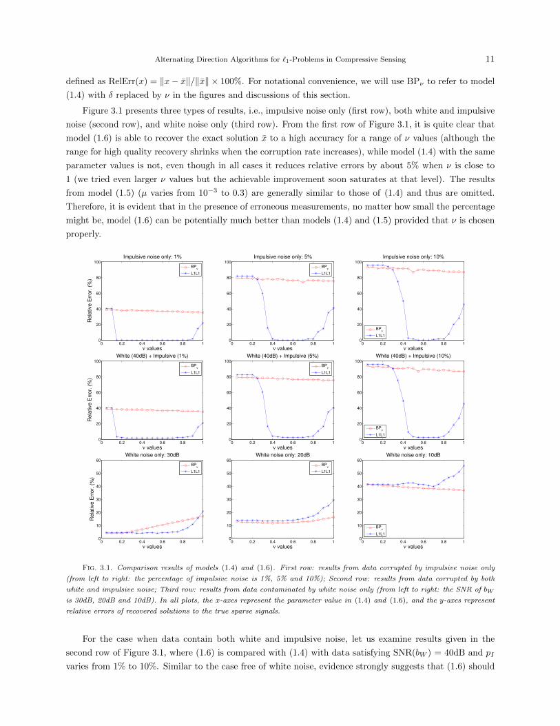
Figure 3.1 presents three types of results, i.e., impulsive noise only (first row), both white and impulsive
noise (second row), and white noise only (third row). From the first row of Figure 3.1, it is quite clear that
model (1.6) is able to recover the exact solution x to a high accuracy for a range of ν values (although the
range for high quality recovery shrinks when the corruption rate increases), while model (1.4) with the same
parameter values is not, even though in all cases it reduces relative errors by about 5% when ν is close to
1 (we tried even larger ν values but the achievable improvement soon saturates at that level). The results
from model (1.5) (µ varies from 10−3 to 0.3) are generally similar to those of (1.4) and thus are omitted.
Therefore, it is evident that in the presence of erroneous measurements, no matter how small the percentage
might be, model (1.6) can be potentially much better than models (1.4) and (1.5) provided that ν is chosen
properly.
0 0.2 0.4 0.6 0.8 10
20
40
60
80
100
ν values
Rela
tive E
rror.
(%
)
Impulsive noise only: 1%
BPν
L1L1
0 0.2 0.4 0.6 0.8 10
20
40
60
80
100
ν values
Impulsive noise only: 5%
BPν
L1L1
0 0.2 0.4 0.6 0.8 10
20
40
60
80
100
ν values
Impulsive noise only: 10%
BPν
L1L1
0 0.2 0.4 0.6 0.8 10
20
40
60
80
100
ν values
Rela
tive E
rror.
(%
)
White (40dB) + Impulsive (1%)
BPν
L1L1
0 0.2 0.4 0.6 0.8 10
20
40
60
80
100
ν values
White (40dB) + Impulsive (5%)
BPν
L1L1
0 0.2 0.4 0.6 0.8 10
20
40
60
80
100
ν values
White (40dB) + Impulsive (10%)
BPν
L1L1
0 0.2 0.4 0.6 0.8 10
10
20
30
40
50
60
ν values
Rela
tive E
rror.
(%
)
White noise only: 30dB
BPν
L1L1
0 0.2 0.4 0.6 0.8 10
10
20
30
40
50
60
ν values
White noise only: 20dB
BPν
L1L1
0 0.2 0.4 0.6 0.8 10
10
20
30
40
50
60
ν values
White noise only: 10dB
BPν
L1L1
Fig. 3.1. Comparison results of models (1.4) and (1.6). First row: results from data corrupted by impulsive noise only
(from left to right: the percentage of impulsive noise is 1%, 5% and 10%); Second row: results from data corrupted by both
white and impulsive noise; Third row: results from data contaminated by white noise only (from left to right: the SNR of bW
is 30dB, 20dB and 10dB). In all plots, the x-axes represent the parameter value in (1.4) and (1.6), and the y-axes represent
relative errors of recovered solutions to the true sparse signals.
For the case when data contain both white and impulsive noise, let us examine results given in the
second row of Figure 3.1, where (1.6) is compared with (1.4) with data satisfying SNR(bW ) = 40dB and pI
varies from 1% to 10%. Similar to the case free of white noise, evidence strongly suggests that (1.6) should

12 J.-F. Yang and Y. Zhang
be the model of choice whenever there might be erroneous measurements or impulsive noise in data even in
the presence of white noise. We did not present the results of (1.5) since they are similar to those of (1.4).
We also tested higher white noise levels and obtained similar results except the quality of reconstruction
deteriorates.
Is model (1.6) still appropriate without impulsive noise? The bottom row of Figure 3.1 contains results
obtained from data with only white noise of SNR(bW ) = 30dB, 20dB and 10dB, respectively. Loosely
speaking, these three types of data can be characterized as good, fair and poor, respectively. As can be seen
from the left plot, on good data (1.4) offers no improvement whatsoever to the basis pursuit model (ν = 0)
as ν decreases. On the contrary, it starts to degrade the quality of solution once ν > 0.25. On the other
hand, model (1.6) essentially does no harm until ν > 0.7. From the middle plot, it can be seen that on fair
data both models start to degrade the quality of solution after ν > 0.7, while the rate of degradation is faster
for model (1.6). Only in the case of poor data (the right plot), model (1.4) always offers better solution
quality than model (1.6). However, for poor data the recovered solution quality is always poor. At ν = 1,
the relative error for model (1.4) is about 38%, representing a less than 5% improvement over the relative
error 42% at ν = 0.05, while the best error attained from model (1.6) is about 40%. The results of (1.5) are
generally similar to those of (1.4) provided that model parameters are selected properly.
The sum of the computational evidence suggests the following three guidelines, at least for random
problems of the type tested here: (i) whenever data may contain erroneous measurements or impulsive
noise, `1-fidelity used by model (1.6) should naturally be preferred over the `2-one used by model (1.4) and
its variants; (ii) without impulsive noise, `1-fidelity basically does no harm to solution quality, as long as
data do not contain a large amount of white noise and ν remains reasonably small; and (iii) when data
are contaminated by a large amount of white noise, then `2-fidelity should be preferred. In the last case,
however, high-quality recovery should not be expected regardless what model is used.
4. Numerical results. In this section, we compare the proposed ADM algorithms, referred to as
PADM and DADM corresponding to the primal- and dual-based algorithms, respectively, with several state-
of-the-art algorithms. In Section 4.1, we give numerical results to emphasize a simple yet often overlooked
point that algorithm speed should be evaluated relative to solution accuracy. In Section 4.2, we describe
our experiment settings, including parameter choices, stopping rules and the generation of problem data
under the MATLAB environment. In Section 4.3, we compare PADM and DADM with FPC-BB [32, 33] — a
fixed-point continuation method with a non-monotone line search based on the Barzilai and Borwein (BB)
steplength [4], SpaRSA [56] — a reconstruction algorithm designed for more general regularizers than the
`1-regularizer, FISTA [5] — a fast IST algorithm that attains an optimal convergence rate in function values,
and CGD [61] — a block coordinate gradient descent method for minimizing `1-regularized convex smooth
function. In Section 4.4 we compare PADM and DADM with SPGL1 [25] — a spectral projected gradient
algorithm for (1.4), and NESTA [6] — a first-order algorithm based on Nesterov’s smoothing technique [38].
We also compare DADM with SPGL1 on the basis pursuit problem in Section 4.5. All experiments were
performed under Windows Vista Premium and MATLAB v7.8 (R2009a) running on a Lenovo laptop with an
Intel Core 2 Duo CPU at 1.8 GHz and 2 GB of memory.
4.1. Relative error versus optimality. In algorithm assessment, the speed of an algorithm is often
taken as an important criterion. However, speed is a relative concept and should be measured in company
with appropriate accuracy, which clearly varies with situation and application. A relevant question here is
what accuracy is reasonable for solving compressive sensing problems, especially when data are noisy as is
the case in most real applications. To address this question, we solved (1.3) with noiseless data and (1.5)
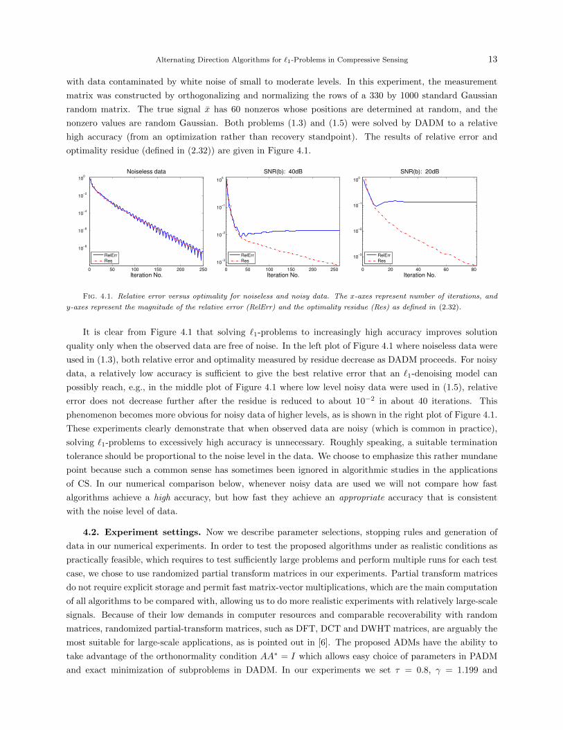
Alternating Direction Algorithms for `1-Problems in Compressive Sensing 13
with data contaminated by white noise of small to moderate levels. In this experiment, the measurement
matrix was constructed by orthogonalizing and normalizing the rows of a 330 by 1000 standard Gaussian
random matrix. The true signal x has 60 nonzeros whose positions are determined at random, and the
nonzero values are random Gaussian. Both problems (1.3) and (1.5) were solved by DADM to a relative
high accuracy (from an optimization rather than recovery standpoint). The results of relative error and
optimality residue (defined in (2.32)) are given in Figure 4.1.
0 50 100 150 200 250
10−8
10−6
10−4
10−2
100
Iteration No.
Noiseless data
RelErr
Res
0 50 100 150 200 250
10−3
10−2
10−1
100
Iteration No.
SNR(b): 40dB
RelErr
Res
0 20 40 60 80
10−3
10−2
10−1
100
Iteration No.
SNR(b): 20dB
RelErr
Res
Fig. 4.1. Relative error versus optimality for noiseless and noisy data. The x-axes represent number of iterations, and
y-axes represent the magnitude of the relative error (RelErr) and the optimality residue (Res) as defined in (2.32).
It is clear from Figure 4.1 that solving `1-problems to increasingly high accuracy improves solution
quality only when the observed data are free of noise. In the left plot of Figure 4.1 where noiseless data were
used in (1.3), both relative error and optimality measured by residue decrease as DADM proceeds. For noisy
data, a relatively low accuracy is sufficient to give the best relative error that an `1-denoising model can
possibly reach, e.g., in the middle plot of Figure 4.1 where low level noisy data were used in (1.5), relative
error does not decrease further after the residue is reduced to about 10−2 in about 40 iterations. This
phenomenon becomes more obvious for noisy data of higher levels, as is shown in the right plot of Figure 4.1.
These experiments clearly demonstrate that when observed data are noisy (which is common in practice),
solving `1-problems to excessively high accuracy is unnecessary. Roughly speaking, a suitable termination
tolerance should be proportional to the noise level in the data. We choose to emphasize this rather mundane
point because such a common sense has sometimes been ignored in algorithmic studies in the applications
of CS. In our numerical comparison below, whenever noisy data are used we will not compare how fast
algorithms achieve a high accuracy, but how fast they achieve an appropriate accuracy that is consistent
with the noise level of data.
4.2. Experiment settings. Now we describe parameter selections, stopping rules and generation of
data in our numerical experiments. In order to test the proposed algorithms under as realistic conditions as
practically feasible, which requires to test sufficiently large problems and perform multiple runs for each test
case, we chose to use randomized partial transform matrices in our experiments. Partial transform matrices
do not require explicit storage and permit fast matrix-vector multiplications, which are the main computation
of all algorithms to be compared with, allowing us to do more realistic experiments with relatively large-scale
signals. Because of their low demands in computer resources and comparable recoverability with random
matrices, randomized partial-transform matrices, such as DFT, DCT and DWHT matrices, are arguably the
most suitable for large-scale applications, as is pointed out in [6]. The proposed ADMs have the ability to
take advantage of the orthonormality condition AA∗ = I which allows easy choice of parameters in PADM
and exact minimization of subproblems in DADM. In our experiments we set τ = 0.8, γ = 1.199 and
14 J.-F. Yang and Y. Zhang
β = 2m/‖b‖1 in (2.13) and (2.16), which guarantee the convergence of PADM given that λmax(A∗A) = 1,
and also work quite well in practice (although suitably larger τ and γ seem accelerate convergence most
of the time). For DADM, we used the default settings in YALL1, i.e., γ = 1.618 and β = ‖b‖1/m. As
described in subsection 4.1, high accuracy is not always necessary in CS problems with noisy data. Thus,
when comparing with other algorithms, we simply terminated PADM and DADM when relative change of
two consecutive iterates becomes small, i.e.,
RelChg ,‖xk+1 − xk‖‖xk‖
< ε, (4.1)
where ε > 0 is a tolerance, although more complicated stopping rules, such as the one based on optimality
conditions defined in (2.32), are possible. Parametric settings of FPC-BB, SpaRSA, FISTA, CGD, SPGL1
and NESTA will be specified when we discuss individual experiments.
In all experiments, we generated data b by MATLAB scripts b = A*xbar + sigma*randn(m,1), where A
is a randomized partial Walsh-Hadamard transform matrix whose rows are randomly chosen and columns
randomly permuted, xbar represents a sparse signal that we wish to recover, and sigma is the standard
deviation of additive Gaussian noise. Specifically, the Walsh-Hadamard transform matrix of order 2j is
defined recursively by
H20 = [1] , H21 =
[1 1
1 −1
], . . . ,H2j =
[H2j−1 H2j−1
H2j−1 −H2j−1
].
It can be shown that H2jH>2j = 2jI. In our experiments, encoding matrix A contains random selected rows
from 2j/2H2j , where 2j/2 is a normalization factor. A fast Walsh-Hadamard transform is implemented in
C language with a MATLAB mex-interface available to all codes compared. In all tests, we set n = 8192 and
tested various combinations of m and p (the number of nonzero components in xbar). In all the test results
given below, we used the zero vector as the starting point for all algorithms unless otherwise specified.
4.3. Comparison with FPC-BB, SpaRSA, FISTA and CGD. In this subsection, we present
comparison results of PADM and DADM with FPC-BB [32, 33], SpaRSA [56], FISTA [5] and CGD [61],
all of which were developed in the last two years for solving (1.5). In this test, we used random Gaussian
spikes as xbar, i.e., the location of nonzeros are selected uniformly at random while the values of the
nonzero components are i.i.d. standard Gaussian. The standard deviation of additive noise sigma and the
model parameter µ in (1.5) are, respectively, set to 10−3 and 10−4. Since different algorithms use different
stopping criteria, it is rather difficult to compare their relative performance completely fairly. Therefore, we
present two classes of comparison results. In the first class of results, we run all the algorithms for about
1000 iterations by adjusting their stopping rules. Then we examine how relative errors and function values
decrease as each algorithm proceeds. In the second class of results, we terminate the ADM algorithms by
(4.1), while the stopping rules used for other algorithms in comparison will be specified below.
Since FPC-BB implements continuation on the regularization parameter but not on stopping tolerance,
we set all parameters as default except in the last step of continuation we let xtol = 10−5 and gtol = 0.02,
which is more stringent than the default setting xtol = 10−4 and gtol = 0.2 because the latter usually
produces solutions of lower quality than that of other algorithms in comparison. For SpaRSA, we used its
monotonic variant, set continuation steps to 20 and terminated it when the relative change in function value
falls below 10−7. The FISTA algorithm [5] is a modification of the well-known IST algorithm [23, 40, 16].
Started at x0, FISTA iterates as follows xk+1 = Shrink(yk − τA∗(Ayk − b), τ/µ
), where τ > 0 is a parameter,
Alternating Direction Algorithms for `1-Problems in Compressive Sensing 15
and
yk =
x0, if k = 0;
xk + tk−1−1tk
(xk − xk−1), otherwise,where tk =
1, if k = 0;1+√
1+4t2k−1
2 , otherwise.
It is shown in [5] that FISTA attains an optimal convergence rate O(1/k2) in decreasing the function value,
where k is the iteration counter. We set τ ≡ 1 in the implementation of FISTA. For the comparison with
CGD, we used its continuation variant (the code CGD cont in the MATLAB package of CGD) and set all
parameters as default except setting the initial µ value to be max(0.01‖A>b‖∞, 2µ) which works better than
the default setting in our tests when µ is small.
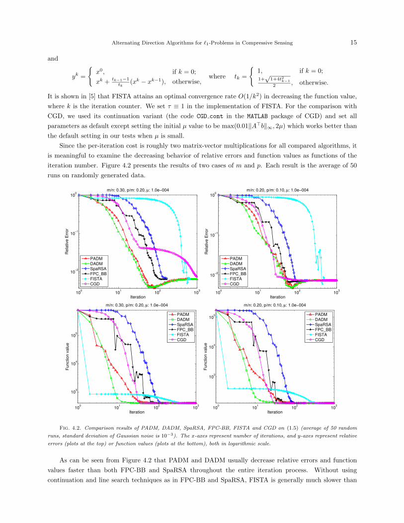
Since the per-iteration cost is roughly two matrix-vector multiplications for all compared algorithms, it
is meaningful to examine the decreasing behavior of relative errors and function values as functions of the
iteration number. Figure 4.2 presents the results of two cases of m and p. Each result is the average of 50
runs on randomly generated data.
100
101
102
103
10−2
10−1
100
Iteration
Re
lative
Err
or
m/n: 0.30, p/m: 0.20, µ: 1.0e−004
PADMDADMSpaRSAFPC_BBFISTACGD
100
101
102
103
10−2
10−1
100
Iteration
Re
lative
Err
or
m/n: 0.20, p/m: 0.10, µ: 1.0e−004
PADMDADMSpaRSAFPC_BBFISTACGD
100
101
102
103
103
104
105
Iteration
Fu
nctio
n v
alu
e
m/n: 0.30, p/m: 0.20, µ: 1.0e−004
PADMDADMSpaRSAFPC_BBFISTACGD
100
101
102
103
103
104
105
Iteration
Fu
nctio
n v
alu
e
m/n: 0.20, p/m: 0.10, µ: 1.0e−004
PADMDADMSpaRSAFPC_BBFISTACGD
Fig. 4.2. Comparison results of PADM, DADM, SpaRSA, FPC-BB, FISTA and CGD on (1.5) (average of 50 random
runs, standard deviation of Gaussian noise is 10−3). The x-axes represent number of iterations, and y-axes represent relative
errors (plots at the top) or function values (plots at the bottom), both in logarithmic scale.
As can be seen from Figure 4.2 that PADM and DADM usually decrease relative errors and function
values faster than both FPC-BB and SpaRSA throughout the entire iteration process. Without using
continuation and line search techniques as in FPC-BB and SpaRSA, FISTA is generally much slower than

16 J.-F. Yang and Y. Zhang
others. In this set of experiments FISTA decreased function values faster at the very beginning, but fell
behind eventually. On the other hand, It was the slowest in decreasing relative errors almost throughout the
entire iteration process. We have found that the slow convergence of FISTA becomes even more pronounced
when µ is smaller. On the first test set represented by the first column of Figure 4.2, both ADMs converge
faster than CGD in decreasing both the relative error and the function value throughout the iteration process.
On the second test set represented by the second column of Figure 4.2, CGD performed more competitively.
However, CGD appeared to be sensitive to the choice of starting points. To demonstrate this, we tested
the algorithms with another starting point x0 = A>b with all the other settings unchanged. The results
for relative errors are given in Figure 4.3. By comparing 4.3 with the first row of Figures 4.2, we observe
that all algorithms exhibited consistent patterns of convergence except CGD whose convergence is slower for
x0 = A>b than for x0 = 0.
100
101
102
103
10−2
10−1
Iteration
Re
lative
Err
or
m/n: 0.30, p/m: 0.20, µ: 1.0e−004
PADMDADMSpaRSAFPC_BBFISTACGD
100
101
102
103
10−2
10−1
Iteration
Re
lative
Err
or
m/n: 0.20, p/m: 0.10, µ: 1.0e−004
PADMDADMSpaRSAFPC_BBFISTACGD
Fig. 4.3. Comparison results of PADM, DADM, SpaRSA, FPC-BB, FISTA and CGD on (1.5) (average of 50 random
runs; standard deviation of Gaussian noise is 10−3; and the common initial point for all algorithms is A>b). The x-axes
represent number of iterations, and y-axes represent relative errors, both in logarithmic scale.
It is worth noting that within no more than 100 iterations PADM and DADM reached lowest relative
errors and then started to increase them, which reflects a property of model (1.5) rather than that of the
algorithms given the fact that the function value kept decreasing. It is also clear that all algorithms eventually
attained nearly equal relative errors and function values at the end. We point out that the performance
of SpaRSA, FPC-BB, FISTA and CGD is significantly affected by the value of µ. In general, model (1.5)
becomes more and more difficult for continuation-based algorithms (SpaRSA, FPC-BB and CGD) as µ
decreases, while the performance of ADMs is essentially unaffected, which can be well justified by the fact
that µ can be set to 0 in both (2.13) and (2.26) in which case both algorithms solve the basis pursuit model
(1.3).
In addition to the results presented in Figure 4.2, we also experimented on other combinations of (m, p)
with noisy data and observed similar phenomenon. As is the case in Figure 4.2, the relative error produced
by the ADM algorithms tends to eventually increase after the initial decrease when problem (1.5) is solved
to high accuracy. This implies, as suggested in Section 4.1, that it is unnecessary to run the ADMs to a
higher accuracy than what is warranted by the accuracy of the underlying data, though this is a difficult
issue in practice since data accuracy is usually not precisely known.
Next we compare PADM and DADM with FPC-BB and SpaRSA for various combinations of (m, p),

Alternating Direction Algorithms for `1-Problems in Compressive Sensing 17
while keeping the noise level at sigma = 1e-3 and the model parameter at µ = 10−4. Here we do not include
results for FISTA and CGD because they have been found to be less competitive on this set of tests. As
is mentioned earlier, without continuation and line search techniques, FISTA is much slower than ADM
algorithms. On the other hand, most of times CGD is slower in terms of decreasing relative errors, as is
indicated by Figures 4.2 and 4.3.
We set all parameters as default in FPC-BB and use the same setting as before for SpaRSA except
it is terminated when relative change in function values falls below 10−4. We set the stopping tolerance
to ε = 2 × 10⁻³ in (4.1) for PADM and DADM. The above stopping rules were selected so that all four
algorithms attain more or less the same level of relative errors upon termination. For each fixed pair (m, p),
we take the average of 50 runs on random instances. Detailed results including iteration number (Iter) and
relative error to the true sparse signal (RelErr) are given in Table 4.1.
Table 4.1
Comparison results on (1.5) (sigma = 10−3, µ = 10−4, average of 50 runs).
n = 8192 PADM DADM SpaRSA FPC-BB
m/n p/m Iter RelErr Iter RelErr Iter RelErr Iter RelErr
0.3 0.1 38.9 6.70E-3 36.4 5.91E-3 103.6 5.61E-3 56.1 5.80E-3
0.3 0.2 50.2 6.52E-3 46.6 5.49E-3 141.3 7.25E-3 94.3 7.66E-3
0.2 0.1 57.2 7.17E-3 54.3 6.25E-3 114.5 7.53E-3 70.5 7.64E-3
0.2 0.2 63.1 8.54E-3 56.1 8.43E-3 180.0 1.68E-2 124.4 2.52E-2
0.1 0.1 85.5 1.17E-2 81.3 1.10E-2 135.6 1.27E-2 84.1 1.35E-2
0.1 0.2 125.4 9.70E-2 105.1 8.99E-2 214.4 1.60E-1 126.4 2.00E-1
Average 70.0 — 63.3 — 148.2 — 92.6 —
As can be seen from Table 4.1, in most cases PADM and DADM obtained smaller or comparable relative
errors in fewer numbers of iterations than FPC-BB and SpaRSA. This is particularly evident for the case
(m/n, p/m) = (0.2, 0.2) where both PADM and DADM obtained notably smaller relative errors, while taking
far fewer iterations than FPC-BB and SpaRSA. At the bottom of Table 4.1, we calculate the average numbers
of iterations required by the four algorithms.
We also tried more stringent stopping rules for the algorithms compared. Specifically, we tried xtol=10−5
and gtol=0.02 in FPC-BB, and terminated SpaRSA when the relative change in the function value falls
below 10−7. The resulting relative errors either remained roughly the same as those presented in Table 4.1
or were just slightly better, while the iteration number required by FPC-BB increased about 50% and that
required by SpaRSA increased more than 100%. For the ADMs, we have found that smaller tolerance values
(say ε = 5× 10⁻⁴) do not necessarily or consistently improve relative error results, while also increasing the
required number of iterations.
4.4. Comparison with SPGL1 and NESTA. In this subsection, we compare PADM and DADM
with SPGL1 and NESTA for solving model (1.4). As before, xbar consists of random Gaussian spikes, and
the standard deviation of additive noise is sigma = 10−3. The model parameter δ in (1.4) was set to be the
2-norm of additive noise (the ideal case). As in the previous experiment, we performed two sets of tests. In
the first set, we ran all compared algorithms for about 400 iterations by adjusting their stopping tolerance
values, while leaving all other parameters to their default values. Figure 4.4 presents average results on 50
random problems, where two combinations of m and p are used. The resulting relative error and residue in
fidelity (i.e., ‖Ax− b‖) are plotted as functions of iterations.
18 J.-F. Yang and Y. Zhang
100
101
102
10−2
10−1
100
Iteration
Re
lative
Err
or
m/n: 0.30, p/m: 0.20,
PADMDADM
SPGL1NESTA
100
101
102
10−1
100
Iteration
Re
lative
Err
or
m/n: 0.20, p/m: 0.20,
PADMDADM
SPGL1NESTA
100
101
102
10−1
100
101
Iteration
Re
sid
ue
: ||A
x−
b|| 2
m/n: 0.30, p/m: 0.20,
PADMDADM
SPGL1NESTA
100
101
102
10−1
100
Iteration
Re
sid
ue
: ||A
x−
b|| 2
m/n: 0.20, p/m: 0.20,
PADMDADM
SPGL1NESTA
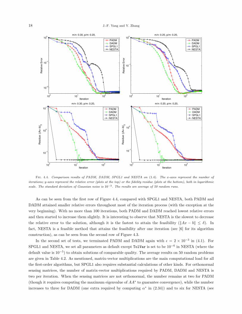
Fig. 4.4. Comparison results of PADM, DADM, SPGL1 and NESTA on (1.4). The x-axes represent the number of
iterations; y-axes represent the relative error (plots at the top) or the fidelity residue (plots at the bottom), both in logarithmic
scale. The standard deviation of Gaussian noise is 10−3. The results are average of 50 random runs.
As can be seen from the first row of Figure 4.4, compared with SPGL1 and NESTA, both PADM and
DADM attained smaller relative errors throughout most of the iteration process (with the exception at the
very beginning). With no more than 100 iterations, both PADM and DADM reached lowest relative errors
and then started to increase them slightly. It is interesting to observe that NESTA is the slowest to decrease
the relative error to the solution, although it is the fastest to attain the feasibility (‖Ax − b‖ ≤ δ). In
fact, NESTA is a feasible method that attains the feasibility after one iteration (see [6] for its algorithm
construction), as can be seen from the second row of Figure 4.3.
In the second set of tests, we terminated PADM and DADM again with ε = 2 × 10⁻³ in (4.1). For
SPGL1 and NESTA, we set all parameters as default except TolVar is set to be 10−6 in NESTA (where the
default value is 10−5) to obtain solutions of comparable quality. The average results on 50 random problems
are given in Table 4.2. As mentioned, matrix-vector multiplications are the main computational load for all
the first-order algorithms, but SPGL1 also requires substantial calculations of other kinds. For orthonormal
sensing matrices, the number of matrix-vector multiplications required by PADM, DADM and NESTA is
two per iteration. When the sensing matrices are not orthonormal, the number remains at two for PADM
(though it requires computing the maximum eigenvalue of AA∗ to guarantee convergence), while the number
increases to three for DADM (one extra required by computing α∗ in (2.34)) and to six for NESTA (see

Alternating Direction Algorithms for `1-Problems in Compressive Sensing 19
[6]). On the other hand, the number required by SPGL1 can vary from iteration to iteration. To accurately
reflect the computational costs consumed by the three algorithms, instead of iteration numbers we present in
Table 4.2 the number of matrix-vector multiplications, denoted by #AAt that includes both A*x and A’*y.
Table 4.2
Comparison results on (1.4) (sigma = 10−3, δ = norm(noise), average of 50 runs).
n = 8192 PADM DADM SPGL1 NESTA
m/n p/m #AAt RelErr #AAt RelErr #AAt RelErr #AAt RelErr
0.3 0.1 82.0 5.82E-3 74.6 7.64E-3 97.7 5.31E-3 297.2 5.74E-3
0.3 0.2 95.6 8.28E-3 90.0 7.36E-3 199.3 7.07E-3 304.3 8.18E-3
0.2 0.1 108.4 7.59E-3 101.0 8.76E-3 149.7 7.46E-3 332.5 6.99E-3
0.2 0.2 120.8 1.04E-2 108.6 1.06E-2 168.2 1.21E-2 336.9 5.77E-2
0.1 0.1 155.7 1.52E-2 149.4 1.42E-2 171.9 1.29E-2 340.6 1.72E-2
0.1 0.2 181.2 8.96E-2 187.8 8.22E-2 184.0 1.13E-1 363.4 3.10E-1
Average 124.0 — 118.6 — 161.8 — 329.2 —
As can be seen from Table 4.2, compared with SGPL1 and NESTA, both PADM and DADM obtained
solutions of comparable quality within smaller numbers of matrix-vector multiplications. At the bottom of
Table 4.2, we present the average numbers of matrix-vector multiplications required by the four algorithms.
4.5. Comparison with SPGL1 on basis pursuit problems. In this subsection, we compare DADM
with SPGL1 on the basis pursuit problem (1.3). The relative performance of PADM and DADM has been
illustrated in the previous comparisons, and DADM is slightly more efficient than PADM. Therefore, we
only present results of DADM. We point out that NESTA can also solve (1.3) by setting δ = 0. However, as
is observable from results in Figure 4.4 and Table 4.2, NESTA is the slowest in decreasing the relative error.
Thus, we only compare DADM with SPGL1. For basis pursuit problems data b is supposed to be noiseless
and higher accuracy optimization should lead to higher-quality solutions. Thus, we terminated DADM with
a stringent stopping tolerance of ε = 10−6 in (4.1). All parameters in SPGL1 are set to be default values.
Detailed comparison results are given in Table 4.3, where, besides relative error (RelErr) and the number of
matrix-vector multiplications (#AAt), the relative residue RelRes = ‖Ax−b‖/‖b‖ and CPU time in seconds
are also given. The results for m/n = 0.1 and p/m = 0.2 are not included in Table 4.3 since both algorithms
failed to recover accurate solutions.
Table 4.3
Comparison results on (1.3) (b is noiseless; stopping rule: ε = 10−6 in (4.1); average of 50 runs).
n = 8192 DADM SPGL1
m/n p/m RelErr RelRes CPU #AAt RelErr RelRes CPU #AAt
0.3 0.1 7.29E-5 4.41E-16 0.44 258.8 1.55E-5 9.19E-6 0.39 114.9
0.3 0.2 7.70E-5 4.65E-16 0.78 431.4 2.50E-5 6.77E-6 1.11 333.4
0.2 0.1 4.26E-5 4.54E-16 0.66 388.2 3.39E-5 1.51E-5 0.45 146.7
0.2 0.2 7.04E-5 4.85E-16 1.15 681.8 1.40E-4 1.03E-5 2.50 791.0
0.1 0.1 4.17E-5 4.86E-16 1.11 698.2 1.25E-4 3.26E-5 0.64 207.9
Average — — 0.83 491.7 — — 1.02 318.8
We observe that when measurements are noiseless and a highly accurate solution is demanded, the
20 J.-F. Yang and Y. Zhang
ADM algorithms can sometimes be slower than SPGL1. Indeed, Table 4.3 shows that DADM is slower
than SPGL1 in two cases (i.e., (m/n, p/m) = (0.3, 0.1) and (0.2, 0.1)) while at the same time getting lower
accuracy. On the other hand, it is considerably faster than SPGL1 in the case (m/n, p/m) = (0.2, 0.2) while
getting higher accuracy. The average CPU time and number of matrix-vector multiplications required by
the two algorithms are presented in the last row of Table 4.3. We note that since SPGL1 requires some
non-trivial calculations other than matrix-vector multiplications, a smaller #AAt number by SPGL1 does
not necessarily lead to a shorter CPU time. We also comment that the relative residue results of DADM are
always numerically zero because when AA∗ = I the sequence xk generated by DADM, applied to (1.3),
satisfies Axk+1 − b = (1− γ)(Axk − b) and thus ‖Ax− b‖ decreases fairly quickly for γ = 1.618.
4.6. Summary. We provided supporting evidence to emphasize that algorithm speed should be eval-
uated relative to solution accuracy. With noisy measurements, solving `1-problems to excessively high
accuracy is generally unnecessary. In practice, it is more relevant to evaluate the speed of an algorithm
based on how fast it achieves an appropriate accuracy consistent with noise levels in data.
We presented extensive experimental results to compare the proposed ADM algorithms with state-of-
the-art algorithms FPC-BB, SpaRSA, FISTA, CGD, SPGL1 and NESTA, using partial Walsh-Hadamard
sensing matrices. Our numerical results show that the proposed algorithms are efficient and robust. In
particular, the ADM algorithms can generally reduce relative errors faster than all other tested algorithms.
This observation is based not only on results presented here using partial Walsh-Hadamard sensing matrices
and Gaussian spike signals, but also on unreported results using other types of sensing matrices (partial
DFT, DCT and Gaussian random matrices) and sparse signals. In practice, however, since relative errors
cannot be measured directly and do not seem to have predictable correlations with observable quantities such
as fidelity residue, it remains practically elusive to take the full advantage of such a favorable property of
the ADM algorithms. Nevertheless, even with unnecessarily stringent tolerance values, the proposed ADM
algorithms are still competitive with other state-of-the-art algorithms.
Our test results also indicate that the dual-based ADMs are generally more efficient than the primal-
based ones. One plausible explanation is that when A is orthonormal, the dual-based algorithms are exact
ADMs, while the primal-based ones are inexact which solve some subproblems approximately. The dual-
based ADMs have been implemented in a MATLAB package called YALL1 [62], which can solve eight different
`1-models including (1.3)-(1.6) and their nonnegative counterparts.
5. Concluding remarks. We proposed to solve `1-problems arising from compressive sensing by first-
order primal-dual algorithms derived from the classic ADM framework utilizing the augmented Lagrangian
function and alternating minimization idea. This ADM approach is applicable to numerous `1-problems
including, but not limited to, the models (1.3)-(1.6) and their nonnegative counterparts. When applied to
the `1-problems, the per-iteration cost of these algorithms is dominated by two matrix-vector multiplications.
Extensive experimental results show that the proposed ADM algorithms, especially the dual-based ones,
perform at least competitively with several state-of-the-art algorithms. On various classes of test problems
with noisy data, the proposed ADM algorithms have unmistakably exhibited the following advantages over
competing algorithms in comparison: (i) they converge well without the help of a continuation or a line search
technique; (ii) their performance is insensitive to changes in model, starting point and algorithm parameters;
and (iii) they demonstrate a notable ability to quickly decrease the relative error to true solutions. Although
the ADM algorithms are not necessarily the fastest in reaching an extremely high accuracy when observed
data are noiseless, they are arguably the fastest in reaching the best achievable level of accuracy when data
contain a nontrivial level of noise. However, to take the full advantage of the ADMs one needs appropriate

Alternating Direction Algorithms for `1-Problems in Compressive Sensing 21
stopping tolerance values which can be difficult to estimate in practice.
The most influential feature of the ADM approach is perhaps its great versatility and its seemingly
universal effectiveness for a wide range of optimization problems in signal, image and data analysis, particular
those involving `1-like regularizations such as nuclear-norm (sum of singular values) regularization in matrix
rank minimization like the matrix completion problem [44, 10, 12], or the total variation (TV) regularization
[46] widely used in image processing. While the nuclear-norm is just an extension of the `1-norm to the matrix
case, the TV regularization can be converted to `1-regularization after introducing a splitting variable [53, 57].
Therefore, the ADM approach is applicable to both nuclear-norm and TV regularized problems (in either
primal or dual form) in a rather straightforward manner so that the derivations and discussions are largely
analogous to those for `1-problems as presented in this paper. Recently, the ADM has also been applied to
TV-based image reconstruction in [22, 57, 49, 37] and to semi-definite programming in [54]. A more recent
application of the ADM approach is to the problem of decomposing a given matrix into a sum of a low-rank
matrix and a sparse matrix simultaneously using `1-norm and nuclear-norm regularizations (see [13]). An
ADM scheme has been proposed and studied for this problem in [60].
Although the ADM approach is classic and its convergence properties have been well studied, its remark-
able effectiveness in signal and image reconstruction problems involving `1-like regularizations has just been
recognized very recently. These fruitful new applications bring new research issues, such as convergence of
certain inexact ADM schemes and optimal choices of algorithm parameters, that should be interesting for
further investigations.
Acknowledgments. We are grateful to two anonymous referees for their valuable comments and sug-
gestions which have helped improve the paper. The first author would like to thank Prof. Bingsheng He of
Nanjing University and Dr. Wotao Yin of Rice University for their helpful discussions. The work of Junfeng
Yang was supported in part by the Natural Science Foundation of China grant NSFC-10971095 and the
Natural Science Foundation of Jiangsu Province BK2008255. The work of Yin Zhang was supported in part
by NSF DMS-0811188 and ONR grant N00014-08-1-1101.
REFERENCES
[1] M. V. Afonso, J. Bioucas-Dias, and M. Figueiredo, Fast image recovery using variable splitting and constrained optimiza-
tion, Available at: http://arxiv.org/abs/0910.4887, 2009.
[2] M. V. Afonso, J. Bioucas-Dias, and M. Figueiredo, A fast algorithm for the constrained formulation of compressive image
reconstruction and other linear inverse problems, Available at http://arxiv.org/abs/0909.3947v1, 2009.
[3] D. Baron, M. Duarte, S. Sarvotham, M. B. Wakin, and R. G. Baraniuk, Distributed compressed sensing, Available at:
http://dsp.rice.edu/cs/DCS112005.pdf.
[4] J. Barzilai, and J. Borwein, Two point step size gradient methods, IMA J Numer. Anal., vol. 8, pp. 141–148, 1988.
[5] A. Beck, and M. Teboulle, A fast iterative shrinkage-thresholding algorithm for linear inverse problems, SIAM J. Imag.
Sci., vol. 2, no. 1, pp. 183–202, 2009.
[6] S. Becker, J. Bobin, and E. Candes, NESTA: A fast and accurate first-order method for sparse recovery, Technical Report,
California Institute of Technology, April, 2009.
[7] J. Cai, S. Osher, and Z. Shen, Linearized Bregman iterations for compressive sensing, UCLA CAM TR08–06.
[8] J. Cai, S. Osher, and Z. Shen, Convergence of the linearized Bregman iteration for `1-norm minimization, UCLA CAM
TR08–52.
[9] E. Candes, J. Romberg, and T. Tao, Stable signal recovery from incomplete and inaccurate information, Commun. Pure
Appl. Math., vol. 59, pp. 1207-1233, 2005.
[10] E. Candes and B. Recht, Exact matrix completion via convex optimization, Submitted, 2008.
[11] E. Candes, J. Romberg, and T. Tao, Robust uncertainty principles: Exact signal reconstruction from highly incomplete
frequency information, IEEE Trans. Inform. Theory, vol. 52, no. 2, pp. 489–509, 2006.

22 J.-F. Yang and Y. Zhang
[12] E. Candes and T. Tao, The power of convex relaxation: Near-optimal matrix completion, Submitted, 2009.
[13] V. Chandrasekaran, S. Sanghavi, P. A. Parrilo, and A. S. Willsky, Rank Sparsity incoherence for matrix decomposition,
http://arxiv.org/abs/0906.2220.
[14] S. S. Chen, D. L. Donoho, and M. A. Saunders, Atomic decomposition by basis pursuit, SIAM J. Sci. Comput., vol. 20,
pp. 33–61, 1998.
[15] I. Daubechies, M. Defriese and C. De Mol, An iterative thresholding algorithm for linear inverse problems with a sparsity
constraint, Commun. Pure Appl. Math., vol. LVII, pp. 1413–1457, 2004.
[16] C. De Mol, and M. Defrise, A note on wavelet-based inversion algorithms, Contemp. Math., 313, pp. 85–96, 2002.
[17] D. Donoho, Compressed sensing, IEEE Trans. Inform. Theory, vol. 52, no. 4, pp. 1289–1306, 2006.
[18] D. Donoho, For most large underdetermined systems of linear equations, the minimal `1-norm solution is also the sparsest
solution, Commun. Pure Appl. Math., vol. 59, no. 7, pp. 907–934, 2006.
[19] J. Douglas, and H. Rachford, On the numerical solution of heat conduction problems in two and three space variables,
Trans. Am. Math. Soc., vol. 82, pp. 421439, 1956.
[20] J. Eckstein, and D. Bertsekas, On the Douglas-Rachford splitting method and the proximal point algorithm for maximal
monotone operators, Math. Program., vol. 55, pp. 293–318, 1992.
[21] M. Elad, Why simple shrinkage is still relevant for redundant representations? IEEE Trans. Inform. Theory, vol. 52, no.
12, pp. 5559–5569, 2006.
[22] E. Esser, Applications of Lagrangian-Based Alternating Direction Methods and Connections to Split Bregman, CAM
Report TR09-31, UCLA, 2009.
[23] M. Figueiredo and R. Nowak, An EM algorithm for wavelet-based image restoration, IEEE Trans. Imag. Process., vol. 12,
no. 8, pp. 906–916, 2003.
[24] M. Figueiredo, R. Nowak, and S. J. Wright, Gradient projection for sparse reconstruction: application to compressed
sensing and other inverse problems, IEEE J. Sel. Top. Signa., vol. 1, pp. 586–597, 2007.
[25] M. Friedlander, and E. Van den Berg, Probing the pareto frontier for basis pursuit solutions, SIAM J. Sci. Comput., vol.
31, no. 2, pp. 890–912, 2008.
[26] M. Fukushima, Application of the alternating direction method of multipliers to separable convex programming, Comput.
Optim. Appl., vol. 1, pp. 93–111, 1992.
[27] D. Gabay, and B. Mercier, A dual algorithm for the solution of nonlinear variational problems via finite-element approx-
imations, Comp. Math. Appl., vol. 2, pp. 17-40, 1976.
[28] R. Glowinski, Numerical methods for nonlinear variational problems, Springer-Verlag, New York, Berlin, Heidelberg,
Tokyo, 1984.
[29] R. Glowinski, and P. Le Tallec, Augmented Lagrangian and operator splitting methods in nonlinear mechanics, SIAM
1989.
[30] R. Glowinski, and A. Marrocco, Sur lapproximation par elements finis dordre un, et la resolution par penalisation-dualite
dune classe de problemes de Dirichlet nonlineaires, Rev. Francaise dAut. Inf. Rech. Oper., R-2, pp. 41-76, 1975.
[31] T. Goldstein, and S. Osher, The split Bregman method for l1 regularized problems, SIAM J. Imag. Sci., vol. 2, no. 2, pp.
323–343, 2009.
[32] E. Hale, W. Yin, and Y. Zhang, Fixed-point continuation for `1-minimization: methodology and convergence, SIAM J.
Optim., vol. 19, no. 3, pp. 1107–1130, 2008.
[33] E. Hale, W. Yin, and Y. Zhang, Fixed-point continuation applied to compressed sensing: implementation and numerical
experiments, J Comput. Math., vol. 28, no. 2, pp. 170–194, 2010.
[34] B. He, L. Liao, D. Han, and H. Yang, A new inexact alternating directions method for monotone variational inequalities,
Math. Progam., Ser. A, vol. 92, pp. 103–118, 2002.
[35] B. He, and H. Yang, Some convergence properties of a method of multipliers for linearly constrained monotone variational
inequalities, Oper. Res. Lett., vol. 23, pp. 151–161, 1998.
[36] M. R. Hestenes, Multiplier and gradient methods, J. Optimiz. Theory App., vol. 4, pp. 303–320, 1969.
[37] C. Li, W. Yin, and Y. Zhang, User’s Guide for TVAL3: TV Minimization by Augmented Lagrangian and Alternating
Direction Algorithms, CAAM Report, 2009.
[38] Y. Nesterov, Smooth minimization of non-smooth functions, Math. Program., Serie A, vol. 103, pp. 127–152, 2005.
[39] Y. Nesterov, Gradient methods for minimizing composite objective function, CORE Discussion Paper 2007/76, 2007.
[40] R. Nowak, and M. Figueiredo, Fast wavelet-based image deconvolution using the EM algorithm, in Proceedings of the
35th Asilomar Conference on Signals, Systems and Computers, vol. 1, pp. 371–375, 2001.
[41] S. Osher, M. Burger, D. Goldfarb, J. Xu, and W. Yin, An iterated regularization method for total variation-based image
restoration, Multiscale Model. Sim., vol. 4, pp. 460–489, 2005.
Alternating Direction Algorithms for `1-Problems in Compressive Sensing 23
[42] G. Plonka and J. Ma, Curvelet-wavelet regularized split Bregman iteration for compressed sensing, International Journal
of Wavelets, Multiresolution and Information Processing, to appear, 2010.
[43] M. J. D. Powell, A method for nonlinear constraints in minimization problems, in Optimization, R. Fletcher, ed., Academic
Press, New York, NY, pp. 283–298, 1969.
[44] B. Recht, M. Fazel, and P. Parrilo, Guaranteed minimum rank solutions of matrix equations via nuclear norm minimiza-
tion, SIAM Rev., to appear, 2010.
[45] R. T. Rockafellar, The multiplier method of Hestenes and Powell applied to convex programming, J. Optimiz. Theory
App., vol. 12, pp. 555–562, 1973.
[46] L. Rudin, S. Osher and E. Fatemi, Nonlinear total variation based noise removal algorithms, Physica D, vol. 60, pp.
259–268, 1992.
[47] J.-L. Starck, E. Candes, and D. Donoho, Astronomical image representation by the curvelet transform, Astron. Astrophys.,
vol. 398, pp. 785–800, 2003.
[48] J.-L. Starck, M. Nguyen, and F. Murtagh, Wavelets and curvelets for image deconvolution: a combined approach, Signal
Process., vol. 83, pp. 2279–2283, 2003.
[49] M. Tao, J.-F. Yang, and B. He, Alternating direction algorithms for total variation deconvolution in image reconstruction,
Optimization Online, 2009.
[50] R. Tibshirani, Regression shrinkage and selection via the Lasso, J. Roy. Statist. Soc., Ser. B., vol. 58, pp. 267-288, 1996.
[51] J. A. Tropp, and A. C. Gilbert, Signal recovery from random measurements via orthogonal matching pursuit, IEEE Trans.
Inform. Theory, vol. 53, no. 12, pp. 4655-4666, 2007.
[52] P. Tseng, Applications of a splitting algorithm to decomposition in convex programming and variational inequalities,
SIAM J. Control Optim., vol. 29, no. 1, pp. 119–138, 1991.
[53] Y. Wang, J.-F. Yang, W. Yin, and Y. Zhang, A new alteranting minimization alrorithm for total variation image recon-
struction, SIAM J. Imag. Sci., vol. 1, pp. 948–951, 2008.
[54] Z. Wen, W. Yin, and D. Goldfarb, Alternating direction augmented Lagrangian methods for semidefinite programming,
Technical Report, IEOR, Columbia University, 2009.
[55] J. Wright, and Y. Ma, Dense error correction via `1-minimization, submitted to IEEE Trans. Inform. theory, 2008.
[56] S. Wright, R. Nowak, and M. Figueiredo, Sparse reconstruction by separable approximation, in Proceedings of the Inter-
national Conference on Acoustics, Speech, and Signal Processing, October 2008.
[57] J.-F. Yang, Y. Zhang, and W. Yin, A fast alternating direction method for TVL1-L2 signal reconstruction from partial
Fourier data, IEEE J. Sel. Top. Signa., Special Issue on Compressive Sensing, vol. 4, no. 2, pp. 288–297, 2010.
[58] W. Yin, S. Osher, D. Goldfarb, and J. Darbon, Bregman iterative algorithms for `1-minimization with applications to
compressed sensing, SIAM J. Imag. Sci., vol. 1, no. 1, pp. 143–168, 2008.
[59] W. Yin, The linearized Bregman method: reviews, analysis, and generalizations, CAAM TR09–02, Rice University.
[60] X. Yuan, and J.-F. Yang, Sparse and low-rank matrix decomposition via alternating direction methods, submitted, 2009.
[61] S. Yun, and K-C Toh, A coordinate gradient descent method for `1-regularized convex minimization, submitted, 2009.
[62] Y. Zhang, J.-F. Yang, and W. Yin, Your ALgorithm for L1, Available at: http://yall1.blogs.rice.edu/
Appendix A. Proof of Theorem 2.1.
Proof. Let (r, x) be any solution of (2.5). From optimization theory, there exists y ∈ Cm such that the
following conditions are satisfied:
r/µ− y = 0, A∗y ∈ ∂‖x‖1 and Ax+ r = b. (A.1)
For convenience, we let r , rk+1, x , xk+1 and y , yk−β(Axk+1 + rk+1− b). For x = xk and y = yk fixed,
the minimizer rk+1 of (2.6) with respect to r satisfies
rk+1/µ+ β(Axk + rk+1 − b− yk/β) = 0. (A.2)
Following the definitions of r, x and y, (A.2) can be rewritten as r/µ − y + βA(xk − x) = 0. Further
considering r/µ− y = 0, we have y − y − βA(xk − x) = (r − r)/µ, and thus
(r − r)∗(y − y − βA(xk − x)
)= ‖r − r‖2/µ ≥ 0. (A.3)
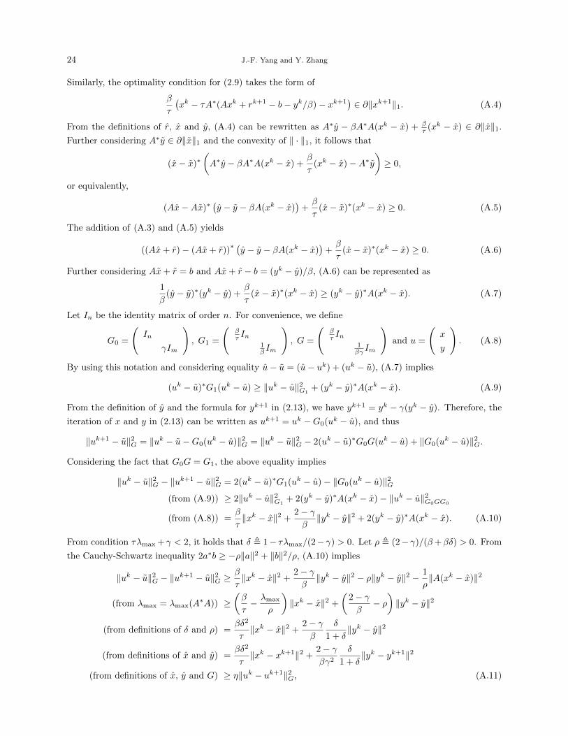
24 J.-F. Yang and Y. Zhang
Similarly, the optimality condition for (2.9) takes the form of
β
τ
(xk − τA∗(Axk + rk+1 − b− yk/β)− xk+1
)∈ ∂‖xk+1‖1. (A.4)
From the definitions of r, x and y, (A.4) can be rewritten as A∗y − βA∗A(xk − x) + βτ (xk − x) ∈ ∂‖x‖1.
Further considering A∗y ∈ ∂‖x‖1 and the convexity of ‖ · ‖1, it follows that
(x− x)∗(A∗y − βA∗A(xk − x) +
β
τ(xk − x)−A∗y
)≥ 0,
or equivalently,
(Ax−Ax)∗(y − y − βA(xk − x)
)+β
τ(x− x)∗(xk − x) ≥ 0. (A.5)
The addition of (A.3) and (A.5) yields
((Ax+ r)− (Ax+ r))∗ (y − y − βA(xk − x)
)+β
τ(x− x)∗(xk − x) ≥ 0. (A.6)
Further considering Ax+ r = b and Ax+ r − b = (yk − y)/β, (A.6) can be represented as
1
β(y − y)∗(yk − y) +
β
τ(x− x)∗(xk − x) ≥ (yk − y)∗A(xk − x). (A.7)
Let In be the identity matrix of order n. For convenience, we define
G0 =
(In
γIm
), G1 =
(βτ In
1β Im
), G =
(βτ In
1βγ Im
)and u =
(x
y
). (A.8)
By using this notation and considering equality u− u = (u− uk) + (uk − u), (A.7) implies
(uk − u)∗G1(uk − u) ≥ ‖uk − u‖2G1+ (yk − y)∗A(xk − x). (A.9)
From the definition of y and the formula for yk+1 in (2.13), we have yk+1 = yk − γ(yk − y). Therefore, the
iteration of x and y in (2.13) can be written as uk+1 = uk −G0(uk − u), and thus
‖uk+1 − u‖2G = ‖uk − u−G0(uk − u)‖2G = ‖uk − u‖2G − 2(uk − u)∗G0G(uk − u) + ‖G0(uk − u)‖2G.
Considering the fact that G0G = G1, the above equality implies
‖uk − u‖2G − ‖uk+1 − u‖2G = 2(uk − u)∗G1(uk − u)− ‖G0(uk − u)‖2G(from (A.9)) ≥ 2‖uk − u‖2G1
+ 2(yk − y)∗A(xk − x)− ‖uk − u‖2G0GG0
(from (A.8)) =β
τ‖xk − x‖2 +
2− γβ‖yk − y‖2 + 2(yk − y)∗A(xk − x). (A.10)
From condition τλmax + γ < 2, it holds that δ , 1− τλmax/(2− γ) > 0. Let ρ , (2− γ)/(β+βδ) > 0. From
the Cauchy-Schwartz inequality 2a∗b ≥ −ρ‖a‖2 + ‖b‖2/ρ, (A.10) implies
‖uk − u‖2G − ‖uk+1 − u‖2G ≥β
τ‖xk − x‖2 +
2− γβ‖yk − y‖2 − ρ‖yk − y‖2 − 1
ρ‖A(xk − x)‖2
(from λmax = λmax(A∗A)) ≥(β
τ− λmax
ρ
)‖xk − x‖2 +
(2− γβ− ρ)‖yk − y‖2
(from definitions of δ and ρ) =βδ2
τ‖xk − x‖2 +
2− γβ
δ
1 + δ‖yk − y‖2
(from definitions of x and y) =βδ2
τ‖xk − xk+1‖2 +
2− γβγ2
δ
1 + δ‖yk − yk+1‖2
(from definitions of x, y and G) ≥ η‖uk − uk+1‖2G, (A.11)
Alternating Direction Algorithms for `1-Problems in Compressive Sensing 25
where η , min(δ2, δ(2−γ)
γ(1+δ)
)> 0. It follows from (A.11) that
(a) ‖uk − uk+1‖G → 0;
(b) uk lies in a compact region;
(c) ‖uk − u‖2G is monotonically non-increasing and thus converges.
From (a), there hold xk−xk+1 → 0 and yk−yk+1 → 0. From yk = yk−1−γβ(Axk+rk−b) and yk−1−yk → 0,
it follows that Axk + rk − b → 0. From (b), uk has a subsequence ukj that converges to u? = (x?; y?),
i.e., xkj → x? and ykj → y?. From the iteration formula (2.7), we have
rk =µβ
1 + µβ
(yk
β−(Axk − b
)+yk−1 − yk
β+A
(xk − xk−1
)).
Taking into consideration xkj → x?, ykj → y?, xk−xk+1 → 0 and yk−yk+1 → 0, the above equality implies
rkj → r? ,µβ
1 + µβ
(y?
β− (Ax? − b)
), j →∞.
Therefore, (r?, x?, y?) is a limit point of (rk, xk, yk). Next we show that (r?, x?, y?) satisfies the optimality
conditions for (2.5). First, from (2.12) and (2.7), we have
yk+1 = yk − γβ(Axk+1 + rk+1 − b) = yk − γβ(Axk+1 − b+
µβ
1 + µβ
(yk
β− (Axk − b)
)),
which is equivalent to
yk − yk+1
γβ+A(xk − xk+1) =
1
1 + µβ
(Axk − b+ µyk
). (A.12)
By taking the limit of (A.12) over kj , it follows that
Ax? − b+ µy? = 0. (A.13)
Second, from the definition of r?, it holds
r?/µ− y? =β
1 + µβ
(y?
β− (Ax? − b)
)− y? =
β
1 + µβ(b−Ax? − µy?) = 0, (A.14)
where the last equality comes from (A.13). Finally, (A.4) can be represented as
β
τ
((I − τA∗A)(xk − xk+1)− τA∗(Axk+1 + rk+1 − b− yk/β)
)∈ ∂‖xk+1‖1. (A.15)
Since xkj → x? and xk+1 − xk → 0, we have xkj+1 = xkj + (xkj+1 − xkj ) → x?. By taking the limit of
(A.15) over kj and further considering Axk + rk− b→ 0, it follows that A∗y? ∈ ∂‖x?‖1, which together with
equations (A.13) and (A.14) imply that (r?, x?, y?) satisfies the optimality conditions for (2.5), i.e.,
r?/µ− y? = 0, A∗y? ∈ ∂‖x?‖1 and Ax? + r? = b. (A.16)
Therefore, we have shown that any limit point of (rk, xk, yk) is an optimal solution of (2.5). Since (A.11)
holds for any optimal solution of (2.5), by letting u = (x, y) = (x?, y?) at the beginning and considering (c),
we get the convergence of uk and thus that of (rk, xk, yk).
Appendix B. Proof of Theorem 2.3.

26 J.-F. Yang and Y. Zhang
Proof. Suppose (x, y) satisfies the optimality conditions for (1.3), i.e., A∗y ∈ ∂‖x‖1 and Ax = b. Let
x , xk+1 and y , yk − β(Axk+1 − b). The optimality condition for (2.18) takes the form of
β
τ
(xk − τA∗(Axk − b− yk/β)− xk+1
)∈ ∂‖xk+1‖1. (B.1)
From the definitions of x and y, (B.1) can be rewritten as A∗y−βA∗A(xk− x)+ βτ (xk− x) ∈ ∂‖x‖1. Further
considering A∗y ∈ ∂‖x‖1 and the convexity of ‖ · ‖1, it follows that
(x− x)∗(A∗y − βA∗A(xk − x) +
β
τ(xk − x)−A∗y
)≥ 0,
or equivalently,
(Ax−Ax)∗(y − y − βA(xk − x)
)+β
τ(x− x)∗(xk − x) ≥ 0. (B.2)
Further considering Ax = b and Ax− b = (yk − y)/β, (B.2) can be represented as
1
β(y − y)∗(yk − y) +
β
τ(x− x)∗(xk − x) ≥ (yk − y)∗A(xk − x),
which is the key inequality for the convergence of (xk, yk). By using the same notation as defined in (A.8)
and similar discussions as in Appendix A, we can prove that
(a) ‖uk − uk+1‖G → 0;
(b) uk lies in a compact region;
(c) ‖uk − u‖2G is monotonically non-increasing and thus converges.
From (a), there hold xk − xk+1 → 0 and yk − yk+1 → 0. From (b), uk has a subsequence ukj that
converges to u? = (x?; y?), i.e., xkj → x? and ykj → y?. Since xkj → x? and ykj−1−ykj = γβ(Axkj−b)→ 0,
it holds Ax? = b. By taking the limit of (B.1) over kj and considering xkj+1 = (xkj+1 − xkj ) + xkj → x?, it
follows that A∗y? ∈ ∂‖x?‖1. Therefore, we have shown that (x?, y?) satisfies the optimality conditions for
(1.3). Since the above discussions apply to any solution u of (1.3), by letting u = (x, y) = (x?, y?) at the
beginning and considering (c), we get the convergence of uk and thus that of (xk, yk).