Alternative Methods for Solving

Heterogeneous Firm Models

Stephen J. Terry∗

April 9, 2014

Abstract

This paper implements and compares four alternative techniques for the solution of het-erogeneous agents business cycle models within the lumpy capital adjustment framework. Thewidespread Krusell Smith algorithm consistently delivers high accuracy and economic impli-cations quantitatively similar to other bounded rationality, projection-based approaches, but itdoes so at the cost of high computational intensity. The Parametrized Distributions and ExplicitAggregation methods yield important speed gains but reduced accuracy. The conceptually dis-tinct Projection plus Perturbation method implies qualitatively similar economic results, evenmore dramatic reductions in computational cost, as well as an important scalability of the ag-gregate state space. A code package implementing each solution method is available online.

Keywords: Heterogeneous Agents, Computational Methods, Lumpy InvestmentJEL: C63, E22, E32

∗stephenjamesterry@gmail.com, Stanford University, Department of Economics, 579 Serra Mall, Stanford, CA94305. All of the code used to produce the results in this paper can be found at Stephen Terry’s website: https:

//sites.google.com/site/stephenjamesterry/. This research was supported by a Bradley dissertation fellowshipfrom the Stanford Institute for Economic Policy Research. This paper was improved by comments from BrentBundick, Itay Saporta-Eksten, and Nick Bloom. A portion of this research was completed as a visitor at the FederalReserve Bank of Richmond, but this paper does not necessarily reflect the views of the Federal Reserve Bank ofRichmond or the Federal Reserve System.

1

1 Introduction

Heterogeneous agent business cycle models offer the attractive possibility of combining a fully

fledged business cycle structure with rich, testable implications for the cross-section of consumer or

firm behavior. However, such frameworks, with seminal examples given by the incomplete markets

model of Krusell and Smith (1998) and the heterogeneous firms model of Khan and Thomas (2008),

pose several practical challenges for researchers. First, their solution and simulation are computa-

tionally intensive. Second, the traditional solution techniques used for these models, such as the

Krusell Smith (KS) algorithm, rely on bounded rationality and aggregation assumptions and must

be evaluated ex-post for the internal consistency of these assumptions. To help guide researchers

around these issues in the practical solution of the incomplete markets model, many papers provide

alternative solution techniques and computational strategies.1 These advances profitably improve

the speed and accuracy of solutions of the incomplete markets model, but the literature lacks a

comprehensive analysis of their applicability to the heterogeneous firms context, which encompasses

a fundamentally different economic and computational environment.2

This paper seeks to provide such a comparison of solution techniques specifically targeted to-

wards the solution of the heterogeneous firms model. The Khan and Thomas (2008) model is a

natural framework on which to base such a comparison because of the large number of papers using

a similar underlying structure.3 The heterogeneous firms framework here combines aggregate un-

certainty in the form of aggregate productivity shocks together with lumpy capital adjustment costs

and a rich cross-sectional distribution of idiosyncratic productivity shocks and capital holdings. I

adapt four existing algorithms to the heterogeneous firms structure, implementing each solution

technique and comparing them along multiple dimensions: their simulated business cycle moments,

cross-sectional investment rate distributions, impulse response functions, internal accuracy, as well

as the computational burden posed by each algorithm. I implement the following four algorithms:

1. the traditional KS approach as first adapted by Khan and Thomas (2008),

2. the Parametrized Distributions (PARAM) algorithm due to Algan et al. (2008, 2010a),

3. the Explicit Aggregation (XPA) method of Den Haan and Rendahl (2010) as first adapted

by Sunakawa (2012),

1See, among others, Algan et al. (2010b), Algan et al. (2008, 2010a), Den Haan and Rendahl (2010), Den Haan(2010b), Maliar et al. (2010), Reiter (2010c), and Young (2010).

2In particular, the heterogeneous firms model requires a discrete investment choice by agents and use of Bellmanequations rather than Euler equations (as in the incomplete markets model) to characterize optimal policies. Theincomplete markets model can also be solved very efficiently at the microeconomic level through use of the EndogenousGrid Points method of Carroll (2006), while such a technique is unavailable for the lumpy investment problem offirms in the heterogeneous firms model.

3See, among others, Gourio and Kashyap (2007), Bloom et al. (2012), Khan and Thomas (2013), Bachmann andBayer (2013), Bachmann and Ma (2012), Bachmann et al. (2013), with earlier work in Khan and Thomas (2003)and Thomas (2002). A complementary literature in heterogeneous agent state-dependent pricing models, typicallydependent on the KS algorithm for solutions, includes papers by Vavra (2014), Klenow and Willis (2007), Knotek(2010), Knotek and Terry (2008), and many others.

2

4. and the Projection plus Perturbation (REITER) solution technique of Reiter (2009).

A quick word about the choice of these four techniques for comparison is in order. The KS

approach is a natural and important choice because of its wide use in the heterogeneous firms

literature to date. The PARAM algorithm is attractive both because it has been studied com-

prehensively in the context of the incomplete markets model but also because it bears conceptual

similarity to another approach, the Backward Induction algorithm of Reiter (2010c). The XPA

approach has been studied previously as a solution method for the heterogeneous firms model in

Sunakawa (2012), and for comparability I rely on that paper’s adaptation of the original Den Haan

and Rendahl (2010) technique.4 Finally, the REITER approach is an important addition to the

algorithms considered here because it is conceptually distinct. The REITER method relies upon a

linear perturbation approach in aggregates together with a rich, discretized projection problem at

the microeconomic level to solve an approximation to the rational expectations equilibrium. For

each solution method, code is readily available online.5

Three main conclusions can be drawn from the comparisons in this paper. First, the KS

algorithm compares very favorably with the other solution techniques considered here. The KS

routine offers a high degree of internal accuracy and delivers economic implications well in line

with those of the other bounded rationality projection-based solution methods. This result should

be interpreted as a favorable robustness check to the large number of papers relying on the KS

algorithm in the heterogeneous firms context, including the original work by Khan and Thomas

(2008). However, these advantages do come at the cost of fairly high computational intensity within

both model solution and simulation steps.

Second, the other two bounded rationality solution techniques based on an approximation of the

aggregate state space and projection methods, PARAM and XPA, both afford important speed gains

relative to KS by avoiding simulation within the solution routine itself. As pointed out by Sunakawa

(2012), these speed gains can open up the possibility of new applications for heterogeneous firms

models, and the business cycle moments, micro-level investment rate distribution, and simulated

impulse responses to productivity shocks are closely in line with those delivered by the KS algorithm.

However, reduced computational burden comes at the cost of less internal accuracy for both the

PARAM and XPA approaches. Furthermore, although model solution time is reduced by use of

these algorithms, simulation for calculation of business cycle moments or impulse response analysis

remains costly.

Third, the REITER approach stands apart from the KS, PARAM, and XPA algorithms for

several reasons. The method is based on an alternative equilibrium concept, i.e. a perturba-

4There are several differences between my work and Sunakawa (2012), however. While that paper usefully drawsout a potential application of speed gains from the XPA algorithm in structural estimation of the aggregate technologyprocess, I focus here instead on a comparison of the solution techniques themselves. Also, my implementation of theXPA approach uses a bias-correction step within the forecasting structure based on a steady-state solution of themodel which is different from the approach in Sunakawa (2012).

5See https://sites.google.com/site/stephenjamesterry/.

3

tion approximation to the full rational expectations equilibrium.6 The resulting solution to the

heterogeneous firms model delivers qualitatively similar economic results as the traditional KS al-

gorithm, although the aggregate dynamics do systematically differ in some ways discussed in more

detail below. In practical terms, the use of perturbation methods delivers speed gains far above

those achieved by either the PARAM or XPA algorithms. Perhaps more significantly, however,

the REITER approach offers scalability of the macroeconomic complexity of heterogeneous agents

models by providing a means for inclusion of a richer aggregate state space than would be currently

tractable using a projection-based approach subject to the curse of dimensionality.

Section 2 lays out the model and calibration, a direct simplification of Khan and Thomas

(2008). Section 3 provides a brief overview of each of the four solution techniques implemented

in the paper. In Section 4, I compare the resulting simulations, impulse responses, accuracy, and

time requirements of each solution method. In an example in Section 5, I extend the baseline

model to include two additional aggregate state variables using the REITER method. Section 6

concludes. Appendix A contains detailed explanations of the solution algorithms as applied to the

heterogeneous firms model, Appendix B contains some practical details on their numerical imple-

mentation as well as additional accuracy checks and figures, Appendix C discusses the simulation

technique used to generate nonlinear impulse responses, and Appendix D discusses an extension to

the aggregate state space of the model solved using the REITER approach.

2 Model and Calibration

The model solved in this code is a simplified version of the model presented and solved in Khan

and Thomas (2008). The simplification involves only the removal of maintenance investment and

trend investment growth, but crucially maintains aggregate uncertainty, the discrete nature of the

investment decision, and idiosyncratic productivity shocks at the microeconomic level. Interested

readers can find much more detail on the assumptions underlying this economic structure in Khan

and Thomas (2008).

2.1 Households

A unit mass continuum of identical households trade a complete set of state-contingent claims, own a

unit mass distribution of firms, and have flow utility given by U(C, 1−N) = log(C)+φ(1−N), φ > 0.

C represents aggregate consumption, and N represents aggregate labor supply. For our purposes,

there are two implications of the household problem from Khan and Thomas (2008) of importance

for the solution of the model. First, firm value maximization is equivalent to maximization of

6Interestingly, in a projection-based solution technique distinct from the projection plus perturbation approachby Reiter (2009, 2010a,b), Gordon (2011) also discusses a means of solving an approximation to the full rationalexpectations equilibrium of the incomplete markets model with the cross-sectional distribution as a state variable,using a dramatically reduced Smolyak grid for the projection routine. Note also that although Reiter (2009) and thispaper’s analysis use a linear perturbation, higher-order approximations of the same equilibrium system are possible,as suggested by Reiter (2010b).

4

dividends weighted by a marginal utility price p. Second, household labor supply optimality and

linear disutility of labor imply a trivial relationship between the wage and price p:

p =1

C(A,µ), w(A,µ) =

φ

p(A,µ).

Above, prices and wages are written in terms of an aggregate state (A,µ) including aggregate

productivity A and a cross-sectional distribution µ of capital and productivity, both of which are

discussed in more detail below.

2.2 Firms

In each period there is a distribution of firms µ(z, k) over idiosyncratic productivity and capital

levels z and k.7 Individual firms are subject to both idiosyncratic and aggregate productivity

shocks, which are exogenous and are assumed to follow independent AR(1) processes in logs:

log(A′) = ρA log(A) + σAεA, log(z′) = ρz log(z) + σzεz

where innovations to both processes are iid N(0, 1). The state vector for an individual firm is given

by (z, k;A,µ), which contains both the idiosyncratic states for that firm as well as an aggregate

state including productivity and all distributional information. Firms also receive a random draw

of fixed capital adjustment costs in each period, discussed below. Conditional upon idiosyncratic

productivity and capital (z, k), a firm that chooses labor input n produces output given by the

decreasing returns to scale technology y(z, k, n,A) = zAkαnν , where α+ ν < 1.

In a rational expectations equilibrium there is a known transition mapping Γµ tracking the

evolution of the cross-sectional distribution, as well as a mapping Γp from the aggregate state to

the marginal utility of the representative household-owner p:

µ′ = Γµ(µ,A), p = Γp(µ,A).

Recall that the wage is a function of the household marginal utility given linear labor disutility, so

that these two aggregate mappings fully characterize the aggregate structure of the economy from

the perspective of an individual firm. Then, in each period, a firm receives a stochastic draw of a

fixed capital adjustment cost ξ, given in units of labor. The firm value function V , adjusted by the

marginal utility of the representative households, is therefore given by

V (z, k;A,µ) = EξV (z, k, ξ;A,µ).

Once a firm receives a draw of a stochastic adjustment cost ξ ∼ G(ξ), the firm faces a choice

between paying the capital adjustment cost or not adjusting the capital stock

V (z, k, ξ;A,µ) = max{−ξp(A,µ)w(A,µ) + V A(z, k;A,µ), V NA(z, k;A,µ)

},

7Note that although I use the term “firm” throughout the paper for simplicity, such models are typically disciplinedby the use of establishment data at the microeconomic level, treating individual establishments as separately operatingbusiness units for the purposes of the model. However, for a recent treatment of a heterogeneous firms structurecentering on the distinction between establishments and firms, see Kehrig and Vincent (2013).

5

where the value upon adjustment V A is given by optimization over investment and labor

V A(z, k;A,µ) = maxk′,n

{p(A,µ)

(zAkαnν − k′ + (1− δ)k − w(A,µ)n

)+ βEΓµ,z′,A′V (z′, k′;A′, µ′)

}.

If a firm chooses not to adjust its capital stock, then it must face a dynamic return V NA which

involves optimization of only the labor input n holding capital levels fixed at the (depreciated) level

from last period:

V NA(z, k;A,µ) = maxn

{p(A,µ) (zAkαnν − w(A,µ)n) + βEΓµ,z′,A′V (z′, (1− δ)k;A′, µ′)

}.

The trivial nature of the discrete choice problem leads to a cutoff rule for capital investment, such

that firms adjust their capital stock if and only if the adjustment cost draw ξ is less than a cutoff

level

ξ∗(z, k;A,µ) =V A(z, k;A,µ)− V NA(z, k;A,µ)

φ,

where the numerator reflects the gains from capital adjustment relative to inaction and the denom-

inator’s adjustment by labor disutility φ is required to convert from marginal-utility to labor units.

Further the distribution of lumpy capital adjustment costs is assumed to be given by G(ξ) = U(0, ξ),

where ξ > 0 indexes the level of the adjustment friction in the economy.

2.3 Equilibrium

An equilibrium represents a set of firm value functions V , V, V A, V NA, firm policies and adjustment

thresholds k′, n, ξ∗, prices p(A,µ), w(A,µ), and mappings Γµ,Γp such that

• Firm capital adjustment choices and policies conditional upon adjustment satisfy the Bellman

equations defining V, V A, V NA above, and therefore firm capital transitions are given by

k′(z, k, ξ;A,µ) =

{k′(z, k;A,µ), ξ < ξ∗(z, k;A,µ)

(1− δ)k, ξ ≥ ξ∗(z, k;A,µ).

• The distributional transition rule used in the calculation of expectations above by firms is

consistent with the aggregate evolution of the distributional state

Γµ(z′, k′) =

∫ ∫ ∫IA(z, k)dµ(z, k)dG(ξ)dΦ(εz)

A(z′, k′, ξ, εz;A,µ) = {(z, k)|k′(z, k, ξ;A,µ) = k′, z′ = ρzz + σzεz},Φ(x) = P(εz ≤ x)

• Aggregate output, investment, and labor are consistent with the current distribution µ and

firm policies:

Y (A,µ) =

∫ ∫zAkαn(z, k, ξ;A,µ)νdµ(z, k)dG(ξ)

I(A,µ) =

∫ ∫(k′(z, k, ξ;A,µ)− (1− δ)k)dµ(z, k)dG(ξ)

N(A,µ) =

∫ ∫n(z, k, ξ;A,µ)dµ(z, k)dG(ξ) +

∫ ∫ ξ∗(z,k;A,µ)

0dG(ξ)dµ(z, k)

6

• Aggregate consumption satisfies the resource constraint

C(A,µ) = Y (A,µ)− I(A,µ).

• The households are on their optimality schedules for savings and labor supply decisions, i.e.

the first order conditions defining marginal utility and wages hold, and the price mapping is

consistent

p(A,µ) = Γp(A,µ) =1

C(A,µ), w(A,µ) =

φ

p(A,µ).

• Aggregate productivity follows the assumed AR(1) process in logs.

2.4 Calibration

The parameter choices used in the solution method comparison below are those chosen by Khan and

Thomas (2008). The parameter choices reflect an annual frequency and positive levels of capital

adjustment costs at the firm level, as summarized in Table 1. Given that this paper is concerned

with the comparison of numerical solution techniques, and that the model is a simplified version of

the original structure, these parameter choices should be taken as purely illustrative.

Table 1: Model Calibration

Parameter Role Value Parameter Role Value

α Capital elasticity 0.256 ν Labor elasticity 0.640β Discount rate 0.977 φ Labor disutility 2.4δ Capital depreciation 0.069 ρA Aggregate persistence 0.859σA Aggregate volatility 0.014 ρz Idiosyncratic persistence 0.859σz Idiosyncratic volatility 0.022 ξ Capital adjustment costs 0.0083

Note: The calibration above is based on Khan and Thomas (2008), Table I, reflecting an annual calibration of theheterogeneous firms model with nonconvex capital adjustment costs.

3 Solution Methods Overview

3.1 Krusell Smith Algorithm

Khan and Thomas (2008) in the original exposition of the heterogeneous firms model use the first

algorithm considered here, the KS approach. Their algorithm extends the one proposed in Krusell

and Smith (1998) for use in the incomplete markets model and bases the general equilibrium

components of the solution on a bounded rationality approach.

When solving their dynamic problem, firms approximate the intractable distribution µ(z, k)

over idiosyncratic productivity and capital with some moments m. In practice, m is chosen to

simply be the mean aggregate level of capital K. Given this approximation, two sets of forecast

rules provide expectations for firms of both the aggregate level of consumption and the evolution

of aggregate capital itself. Therefore, the intractable state vector (z, k;A,µ) for the firm problem

7

discussed above is replaced by (z, k;A,m), and the transition and price mappings are replaced by

forecast rules m′ = Γm and p = Γp. In practice, the forecast rules are assumed to take a loglinear

form conditional upon aggregate productivity, although the algorithm allows for more flexibility in

theory.

Solution of the model involves repeated simulation to obtain a fixed point on the forecast

mappings for firms. First, a particular set forecast rules is assumed, allowing for the creation of

value functions for the idiosyncratic firm problems using the simplified state space (z, k;A,m).

Then, given the idiosyncratic firm value functions, the model is simulated. Throughout this paper

unless otherwise noted, aggregate and productivity shocks in the KS method, as well as the PARAM

and XPA techniques, are discretized using the Markov chain approximation process of Tauchen

(1986). Also, unless otherwise noted, simulation of the cross-sectional distribution of productivity

and idiosyncratic capital makes use of the nonstochastic or histogram-based approach in Young

(2010) rather than relying on simulation of individual firms. This histogram-based simulation

technique avoids the sampling error associated with individual firm simulation and in practice is

less computationally burdensome. In each period, market-clearing consumption must be found

by repeated reoptimization of firm policies given a guessed price level, the currently simulated

histogram of firm states, and continuation values and expectations as dictated by the firm values

computed using the current forecast rule guess. Finally, after simulation is complete, the forecast

rules are updated on the simulated aggregates. The entire process repeats until a fixed point is

achieved in the forecast rules. Further details on the KS solution algorithm, as well the practical

choices surrounding the numerical solution of the model can be found in Appendixes A and B.

3.2 Parametrized Distributions Algorithm

The PARAM algorithm is based on the work of Algan et al. (2008, 2010a), which was done in the

context of the incomplete markets model, and the solution technique bears heavy resemblance to

the Backward Induction algorithm of Reiter (2010c). To my knowledge, this paper represents the

first application of the PARAM algorithm to a version of the Khan and Thomas (2008) model.

The PARAM approach, like the KS method, relies upon a bounded rationality assumption, the

replacement of the cross-sectional distribution µ(z, k) with a set of moments m in the dynamic

problem of an individual firm.

However, and contrasting with the KS assumption of forecast rules Γm and Γp for the aggregate

moments and prices, the PARAM approach instead relies upon a set of “reference moments” mref ,

equal to the higher-order centered moments of the cross-sectional distribution of firm capital, con-

ditional upon idiosyncratic productivity. The moments m included in the approximate state for

firm dynamic problems are either a subset of or implied by the reference moments mref , and they

can be drawn from a steady-state solution of the model with no aggregate uncertainty if solution

of the model without simulation is desired.

Solution of the model involves value function iteration with the simplified state space of (z, k;A,m).

8

Given a guess for the firm value function which can be used in construction of the continuation

value in the firm Bellman equations, optimization and calculation of the next iteration of the

value function requires calculation of two objects: market-clearing price p(A,m) for construction of

current-period returns, and next-period moments m′ for input into continuation values. Both p and

m′ can be computed within the value function iteration step quite naturally by using fixed point

iteration. After guessing values for (p,m′), firm policies are computable, and implied aggregates

can be obtained by integrating over the cross-sectional distribution of firm-level productivity and

capital (z, k). Such integration is the key step within the PARAM algorithm and is performed

numerically using flexible exponential functional forms for the density of the model which exactly

match the aggregate moments m together with the higher-order reference moments in the cross-

section. Iteration on prices and next-period moments continues until a fixed point is achieved, at

which point the next value function iteration step is taken. Once the value function converges, the

model is solved.

Note that crucially the PARAM approach does not require simulation and therefore leads to

large time savings relative to the KS algorithm’s solution. However, if desired, new values for

reference moments can be computed from simulation and updated until an outside fixed point is

achieved, similar to the KS technique. In either case, however, simulation in each period requires

a fixed-point iteration routine over market-clearing prices and next-period moments, similar to the

process within the model solution step and involving integration over parametrized cross-sectional

densities. See Appendix A for further details on the PARAM algorithm, as well as the functional

forms used for the assumed cross-sectional densities.8

3.3 Explicit Aggregation Algorithm

The XPA solution method relies upon the techniques suggested by Den Haan and Rendahl (2010),

as first adapted and applied to the heterogeneous firms model by Sunakawa (2012). The algorithm

is essentially identical to the KS method, also making use of a bounded rationality assumption

replacing the aggregate state space (A,µ) with an approximation based on moments (A,m) and

using forecasting rules Γm and Γp for the aggregate moments and prices.

However, there is one main difference between the two techniques. XPA replaces the simulation

step of the KS routine with an aggregation across a fixed cross-sectional distribution which is made

feasible through the substitution of aggregate states into idiosyncratic policies. In other words,

once value functions and policies are obtained based on a simplified state space of (z, k;A,m)

and the posited forecast rules, market-clearing prices are obtained by integrating policies over the

constant exogenous ergodic distribution of z and ignoring heterogeneity in idiosyncratic capital

k. Afterwards, the forecast rules can be updated from the moments and prices generated in this

manner until a fixed point is achieved.

8The algorithm laid out in Appendix A, as well as the code posted online, allows for use of fixed steady-statereference moments and alternatively for updating of these moments through simulation. I use only the former in thispaper, because doing so by itself already yields economic implications similar to the KS and XPA techniques.

9

As the original work by Den Haan and Rendahl (2010) noted, substitution of aggregate states

into idiosyncratic policies creates a Jensen’s inequality-type bias in the forecast system (and hence

the resulting aggregate solution) which can be ameliorated in a straightforward way by use of

information from the steady-state solution.9 Importantly, however, avoiding simulation within the

solution step also allows for large time savings, as emphasized and put to interesting practical use

for structural estimation of technology shocks by Sunakawa (2012).

3.4 Projection plus Perturbation Algorithm

The REITER algorithm is based on the work of Reiter (2009) in the context of the incomplete

markets model. The REITER approach has gained traction recently in the analysis of models

with nonconvex costs and heterogeneity, being used in Costain and Nakov (2011) and Reiter et al.

(2009). To my knowledge, this paper is the first application of the approach to a version of the

Khan and Thomas (2008) model by itself, although it should be noted that Reiter et al. (2009)

analyzes a similar sticky-capital environment with the addition of a New Keynesian sticky-price

structure.

The REITER solution method departs in two important ways from the KS, PARAM, and XPA

approaches. First, and importantly, the algorithm solves an approximation to the full, rational

expectations equilibrium of the model rather than relying upon a bounded rationality assumption

to reduce the state space using a set of moments. Therefore, the REITER method can be used as a

check on the bounded rationality assumptions of the KS, PARAM, and XPA algorithms. Second,

the REITER method relies upon linear perturbation of the model around the steady-state of a

model with no aggregate uncertainty, although it still preserves idiosyncratic nonlinearity through

a discretization of the firm-level problem. By contrast, the methods considered so far have relied

upon global solution techniques, conditional on their bounded rationality assumptions. Importantly,

such a perturbation approach leads to drastically reduced computational requirements, although of

course the global nature of the other solutions must serve as a useful cross-check for large simulated

fluctuations away from the steady-state solution.

The REITER approach relies upon three steps. The first step imposes almost trivial compu-

tational cost: the solution of a steady-state model with no aggregate uncertainty but maintaining

micro-level nonlinearity, using a discretization or histogram for idiosyncratic states (z, k). Then,

the second step writes the full, discretized rational expectations equilibrium as the solution to a

system of nonlinear equations F . The system is a function of current and lagged values of a large

endogenous vector Xt, as well as some exogenous aggregate shocks εt. In the application to the het-

erogeneous firms model, the endogenous vector includes aggregate productivity, the cross-sectional

histogram weights on each idiosyncratic point, firm values at a set of discrete points, as well as some

implied model aggregates including price, output, investment, and labor. Therefore, the system F

9In particular, the forecast rules can be adjusted so that they are consistent with a fixed point at the steady-statelevels of capital and price.

10

must take into account Bellman equations, distributional transitions, and equilibrium conditions.

The third step involves the application of standard techniques for the solution of dynamic linear

rational expectations systems, such as the method of Sims (2002) or Christiano (2002), to the

solution of the heterogeneous firms model. Through numerical differentiation, the system F can

be written as a linear approximation around the steady-state solution of the model, and then the

standard methods for the solution of linear models may be applied. Further discussions of the

details of the REITER solution method can be found in Appendix A.

4 Comparing Solutions

This section compares the four alternative solutions to the heterogeneous firms model along multiple

dimensions: reported business cycle aggregate series and moments, impulse response functions to

an aggregate productivity shock, microeconomic moments of investment rates, internal accuracy

and diagnostic statistics, and finally a comparison of computational time. Unless otherwise noted,

comparisons across methods are conducted with comparable levels of computational intensity, i.e.

the projection grid ranges and densities do not vary across methods, similar interpolation and

optimization techniques are used when solving Bellman equations, and of course random exogenous

shocks are held constant during simulation across methods.10 Specific details about the numerical

choices made are available in Appendix B. Appendix C contains details on the procedure used to

simulate impulse responses in the nonlinear discretized models.

4.1 Unconditional Simulation: Business Cycle Moments and Micro Investment

To begin the comparison, Figure 1 plots a representative 100-period portion of larger 2000-period

simulation of the solutions from each technique, displaying log aggregate output, investment, la-

bor input, exogenous productivity, and market-clearing price. For strict comparability we must

maintain identical driving processes across the discretized aggregate productivity series of the KS,

PARAM, and XPA methods and the REITER linearized solution, which by contrast takes contin-

uous local shocks to aggregate productivity. To accomplish this, a set of continuous productivity

shocks duplicating the discretized aggregate productivity process were trivially computed and input

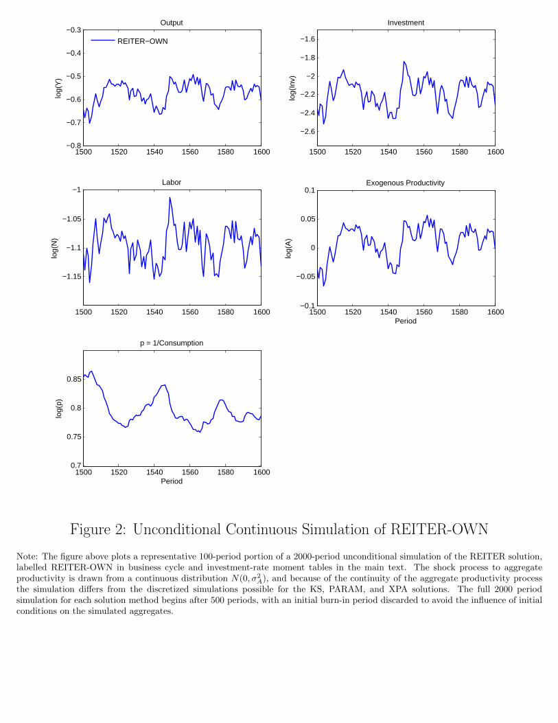
into the REITER solution to produce Figure 1. Figure 2, by contrast, displays business cycle ag-

gregates from a representative portion of a distinct unconditional simulation, with identical length,

of the REITER solution based on continuous exogenous productivity shocks drawn from N(0, σ2A),

which is labelled REITER-OWN in discussion of business cycle moments below.

10The exception to this rule is a higher density of the discretized cross-sectional distribution of capital used whensolving the REITER method. The linearization of the equilibrium centers crucially around this distribution and isslightly more sensitive to grid size than the projection-based KS, PARAM, or XPA methods. Since accuracy statisticsare not directly compared between the REITER method and other methods, and since notwithstanding the highergrid size the REITER method simulation times are still substantially lower than for other techniques, as discussedbelow, the difference does not affect the qualitative conclusions of the paper. More details are available in AppendixB.

11

Table 2: Unconditional Simulation Differences

Method Output Investment Labor Price

Mean % Difference from KS

PARAM -0.2760 -0.6892 -0.1144 0.1751XPA 0.0053 0.2849 0.0079 0.0118

REITER -0.1736 0.0710 -0.1219 0.0527

Note: Mean percentage differences between the business cycle simulations for the PARAM, XPA, and REITERsolutions over a 2000-period unconditional simulation, relative to an analogous KS simulation are reported in thistable, with columns representing the average value of 100(log(Xmethod

t ) − log(XKSt )) for each solution method and

series Xt. The exogenous aggregate productivity process reflects a Markov chain discretized using the Tauchen(1986) procedure and is held constant across solution methods during the simulation. To achieve this, an identicalsimulated discretized productivity process is input directly into the KS, PARAM, and XPA solutions, while a seriesof continuous aggregate shocks exactly replicating the discretized productivity process is input into the REITERsolution. For each method, the full 2000 period simulation for each solution method begins after 500 periods, withan initial burn-in period discarded to avoid the influence of initial conditions on the simulated aggregates.

Although the simulated fluctuations are quite similar across solution methods in Figure 1, a few

patterns are immediately visible to the naked eye. First, mean differences between the simulated

aggregates appear small. This result is confirmed by Table 2, which reports average differences

between each series and a KS method baseline of well under 0.7% in magnitude throughout the

simulation. However, and especially for the price and labor series, there appear to be some differ-

ences in volatility between the projection-based solutions KS, PARAM, and XPA and the linearized

REITER method. In particular, the REITER-simulated price (labor) series are slightly less (more)

volatile than the other three simulations, a fact that is reflected in the business cycle moments

available in Tables 3 and 4.

Table 3: HP-Filtered Volatilities

Method Output Investment Labor Productivity Price

KS (0.02526) 3.9313 0.6937 0.5740 0.3780PARAM (0.023778) 3.7041 0.6518 0.6098 0.4371

XPA ( 0.023928) 3.7098 0.6538 0.6060 0.4380REITER (0.026462) 3.7757 0.8774 0.5479 0.2372

REITER - OWN (0.024431) 3.7909 0.8748 0.5499 0.2448

Note: The business cycle volatility moments of the KS, PARAM, XPA, and REITER solutions over a 2000-periodunconditional simulation are reported in this table in the first four rows. The first column reports, in parentheses,the standard deviation of the HP-filtered log aggregate output series. The second through fifth columns reportthe ratio of the standard deviation of the aggregate HP-filtered log investment, labor, exogenous productivity, andprice series to the output standard deviation in the first row. Following Khan and Thomas (2008), the HP-filter usessmoothing parameter 100. In the first four rows, the exogenous aggregate productivity process reflects a Markov chaindiscretized using the Tauchen (1986) procedure and is held constant across solution methods during the simulation.To achieve this, an identical simulated discretized productivity process is input directly into the KS, PARAM, andXPA solutions, while a series of continuous aggregate shocks exactly replicating the discretized productivity processis input into the REITER solution. In the fifth row, analogous moments from a continuous shock simulation forthe REITER solution is reported, labelled “REITER-OWN.” For each case, the full 2000 period simulation for eachsolution method begins after 500 periods, with an initial burn-in period discarded to avoid the influence of initialconditions on the simulated aggregates.

12

The standard set of HP-filtered business cycle volatilities and ratios in Table 3 reveals broadly

similar and familiar variability of aggregate output, as well as relative volatilities of productivity,

across all four solution methods.11 Furthermore, for all series, flow investment is at least several

times more volatile than output, with the volatility of consumption (equal to that of price, given the

log transformation of p = 1C used here) smallest due to the smoothing effects of general equilibrium.

Importantly, however, as noted above, the REITER solution delivers higher variability of labor

as well as lower variability of prices or consumption than the projection-based techniques. This

phenomenon is not due to the use of discrete shocks with the linearized REITER solution, as

the same conclusion can be drawn from the moments of the REITER-OWN simulation based on

continuous shocks. Rather, the moderate price-dampening appears to be an implication of the use

of local perturbation techniques rather than projection in the aggregate state space.

Business cycle correlations with output reported in Table 4 reveal a similar message: broad

similarities among the KS, PARAM, and XPA methods, with a bit less (more) comovement of price

(labor) with aggregate output in the REITER simulations. As I will argue below, the perturbation

approach of the REITER technique offers attractive scalability of the complexity of the aggregate

state space, but the potential for differences in macroeconomic volatilities relative to the KS method

in the heterogeneous firms context should be kept in mind by researchers using the technique.

Table 4: HP-Filtered Correlation with Output

Method Output Investment Labor Productivity Price

KS 1.0000 0.9779 0.9660 0.9999 -0.8806PARAM 1.0000 0.9734 0.9481 0.9974 -0.8811

XPA 1.0000 0.9702 0.9434 0.9962 -0.8709REITER 1.0000 0.9845 0.9769 0.9952 -0.5921

REITER-OWN 1.0000 0.9845 0.9751 0.9953 -0.5919

Note: The business cycle correlations for the KS, PARAM, XPA, and REITER solutions over a 2000-period uncon-ditional simulation are reported in this table in the first four rows. The first column reports the correlation of theHP-filtered log aggregate output series with itself, 1. The second through fifth columns report the correlation of theaggregate HP-filtered log investment, labor, exogenous productivity, and price series with the filtered output series.Following Khan and Thomas (2008), the HP-filter is performed with smoothing parameter 100. In the first fourrows, the exogenous aggregate productivity process reflects the Markov chain discretized using the Tauchen (1986)procedure and is held constant across solution methods during the simulation. To achieve this, an identical simulateddiscretized productivity process is input directly into the KS, PARAM, and XPA solutions, while a series of contin-uous aggregate shocks exactly replicating the discretized productivity process is input into the REITER solution. Inthe fifth row, analogous moments from a continuous shock simulation for the REITER solution is reported, labelled“REITER-OWN.” For each case, the full 2000 period simulation for each solution method begins after 500 periods,with an initial burn-in period discarded to avoid the influence of initial conditions on the simulated aggregates.

One important advantage of the heterogeneous agents approach is the possibility of disciplin-

ing the parametrization of a model with evidence from the micro-level distribution of investment

11Comparison of Tables 3 and 4 here to Table IV of Khan and Thomas (2008) will reveal some moderate quantitativedifferences between the business cycle moments of this paper’s KS simulation and their “GE lumpy” model. Given theremoval of maintenance investment for expositional clarity, and the distinct discretizations of aggregate productivity,we would not expect identical results. Therefore, it should be emphasized that the correct analysis of the results inthis paper is based on relative comparisons across methods, rather than direct comparison with Khan and Thomas(2008).

13

rates. A number of cross-sectional moments can be computed for each period of the unconditional

simulation of the model within each solution method, based directly on the Young (2010)-style

simulated histograms for the KS and XPA solutions, the parametrized cross-sectional densities and

coefficients of the PARAM method, and the endogenous discretized vector of histogram weights

available directly from the REITER simulation. Here, we focus on the moments analyzed by Khan

and Thomas (2008), including the prevalence of inaction, large positive or negative investment

“spikes,” and the overall likelihood of positive or negative investment. Table 5 reports the mean

levels of these statistics, together with the first and second moments of the investment-rate dis-

tribution. Comfortingly, the methods deliver broadly similar implications for the cross-section of

investment, although the cross-sectional dispersion of investment rates is lower for the REITER

solution.12 Around three-quarters of firms are inactive in each period, with around one-fifth of firms

exhibiting both positive investment spikes or positive investment overall. Much smaller proportions

of observations see negative investment spikes or rates.13

Table 5: Microeconomic Investment-Rate Moments

KS PARAM XPA REITER REITER-OWN

Simulated Mean Valueik 0.0891 0.0887 0.0903 0.0797 0.0364

σ(ik

)0.2224 0.2247 0.2290 0.0939 0.0624

P( ik = 0) 0.7348 0.7411 0.7405 0.7706 0.7169P( ik ≥ 0.2) 0.1904 0.1982 0.1906 0.1628 0.0904

P( ik ≤ −0.2) 0.0234 0.0255 0.0245 0.0101 0.0472P( ik > 0) 0.2209 0.2167 0.2152 0.1925 0.1196P( ik < 0) 0.0443 0.0423 0.0443 0.0397 0.0755

Note: The rows of the table above report the mean value, across periods, of the indicated microeconomic momentof the cross-sectional distribution of investment rates i

kfrom a 2000-period unconditional simulation of the KS,

PARAM, XPA, and REITER methods. The first row reports the level of investment rates, the second row thecross-sectional standard deviation of investment rates, the third column the probability of investment inaction, thefourth (fifth) columns the probability of positive (negative) investment spikes larger in magnitude than 20%, andthe sixth (seventh) columns the probability of strictly positive (negative) investment rates. The first four columnsreport values from simulations based on identical discretized aggregate productivity processes, while the fifth column,labelled REITER-OWN reports a distinct simulation with continuous aggregate productivity shocks input into theREITER solution. In all columns, the full 2000 period simulation for each solution method begins after 500 periods,with an initial burn-in period discarded to avoid the influence of initial conditions on the simulated aggregates.

12The one exception to this pattern is the REITER-OWN simulation, which is subject to a distinct simulationof continuously varying aggregate productivity shocks, and is not directly comparable to the discretized aggregateproductivity simulation used to produce the other microeconomic moments in the first four columns of the table.

13It’s important to note that, as opposed to the model in Khan and Thomas (2008) which allows for costlessmaintenance investment, the simplified structure here results in higher levels of investment inaction and lower levelsof negative investment, because firms do not have a low-cost option for engaging in small adjustments to their capitalstock. Consistently across solution methods, the environment here therefore delivers moments broadly similar tothose of the “Traditional Model” of Table II in Khan and Thomas (2008).

14

4.2 Impulse Response Functions

Now we turn to a comparison of the heterogeneous firms solutions based on conditional responses,

or impulse response analysis, rather than unconditional simulations. At this point, some concrete

decisions must inevitably be made about the manner in which to simulate the underlying object

of interest, i.e. the average change in the forecast of a given series in response to a shock to

aggregate productivity of a certain size. Two considerations will always face a researcher working

with nonlinear discretized models like those considered here. First, given the nonlinear structure of

the KS, PARAM, and XPA solutions, the average conditional response to a shock will depend both

upon initial conditions and upon the size of the shock. Second, we may wish to consider a shock

scaled to a certain average size, such as the calibrated standard deviation of the underlying true

aggregate productivity process, but a discrete Markov chain only admits discrete innovations in the

aggregate productivity series. Neither challenge is present with a linearized solution such as that

available for the REITER method, since in that case a classical impulse response is computable

directly from the coefficients defining the model solution, and the local linearity guarantees that

for small perturbations the impulse response scales directly with shock size.

Table 6: IRF Simulation Differences

Method Output Investment Labor Price

Mean % Difference from KS

PARAM -0.1093 -0.3188 -0.0853 0.0248XPA -0.1035 -0.2742 -0.0550 0.0533

REITER -0.0413 0.3062 0.0905 0.1354

Note: Mean percentage differences between the impulse response simulations for the PARAM, XPA, and REITERsolutions, relative to an analogous KS impulse response simulation are reported in this table, with entries representingthe average percentage value of xmethodt − xKSt for each solution method method and impulse response xmethodt ,averaged over the post-shock period. The exogenous aggregate productivity impulse response is simulated as suggestedby Koop et al. (1996), discussed in more detail in Appendix C, and involves the computing the average log differencebetween 2000 independent simulations of 50-period length, with and without positive productivity shocks.

To create an approximation to the average conditional response in our context, we therefore

simulate the “generalized nonlinear impulse responses” of Koop et al. (1996), although for simplic-

ity we refer to these simply as “impulse responses.” The details of this approach are contained

in Appendix C, but a brief overview is in order here. The approach relies upon a large number

of pairs of simulations, with one “shock” simulation and one “no shock simulation.” Within each

pair, the two simulations are run under identical exogenous shock processes, with one difference.

At a designated period after some initialization range, we impose a positive shock to aggregate

productivity in the shock simulation, allowing the aggregates to evolve as normal afterwards. The

average percentage difference, across simulation pairs, between the shocked and no shock simula-

tions provides a reasonable approximation to the average innovation to a given series in response

to a productivity shock.

15

To generate a flexibly-sized aggregate shock using discretized productivity, we simply convexify

the shock arrival within each simulation pair described above, imposing a shock only with a prob-

ability calculated to generate any desired average change in aggregate productivity. The details of

this additional modification, as well as Figure C1 comparing the virtually identical linearized and

simulated impulse responses for the REITER method are again available in Appendix C.

Figure 3 plots the impulse response to a one-standard deviation (1.4%) average positive ag-

gregate productivity shock for aggregate output, investment, labor, and price. The responses are

qualitatively identical: an increase in aggregate productivity leads immediately to a jump in output,

labor, and investment, together with an increase in consumption (reduction in price) that dissipates

more gradually than the other series. Unsurprisingly, investment responds most strongly, with more

moderate responses from other aggregates. Table 6 reports mean percentage differences between

the conditional responses in the KS case and the PARAM, XPA, and REITER simulations, reveal-

ing little difference on average, all under a third of a percent in magnitude. Unsurprisingly, given

the unconditional business cycle patterns considered above, the price (labor) response is smaller

(stronger) for the REITER method than for the projection based KS, PARAM, and XPA methods.

4.3 Accuracy Statistics

As described above, firms making investment choices in the bounded rationality KS, PARAM,

and XPA solution techniques must rely upon the simplified aggregate state space (A,K) to form

expectations both about market-clearing prices today p, as well as the aggregate capital level in

the next period K ′. In the case of the KS and XPA solutions, firms make use of explicit log linear

forecast rules for both quantities, conditional upon the discretized aggregate productivity state

today. The PARAM method does not make available an explicit forecast rule, but PARAM does

endogenously generate within the solution step a mapping over some projection grid on (A,K)

to clearing levels of (p,K ′), as discussed in more detail in Appendix A. By linearly interpolating

this mapping we can generate a forecast system for price and aggregate capital from the PARAM

solution.

There are several metrics commonly used in the heterogeneous agents literature to evaluate

the internal accuracy of the expectations embedded in bounded rationality forecasting rules. For

each forecast system, it is natural to compare several horizons of forecasts to gauge their inter-

nal accuracy, and the one-step ahead forecast accuracy is commonly evaluated using the R2 of

the regressions, as in Khan and Thomas (2008) or the original Krusell and Smith (1998) analysis.

Similarly, the root mean squared error (RMSE) in percentage terms, can be computed from the

one-step ahead capital and current-period price forecast rules. Both the R2 and RMSE statistics

are reported in Appendix B in Table B2, conditional upon the realized discretized level of aggregate

productivity A and based on the same common-across-methods 2000-period unconditional simu-

lation of the aggregate productivity process used above for the comparison of business-cycle and

micro-level investment moments. Appendix Figure B2 provides a comparison plot.

16

Table 7: Accuracy Statistics for Forecast Rules

Max DH, K ′ Mean DH, K ′ Max DH p Mean DH p

KS 0.6199 0.1909 0.2155 0.0411PARAM 2.5986 0.4657 1.6889 0.2851

XPA 3.7564 0.7417 1.5376 0.3008

Note: The table above reports internal accuracy statistics based on unconditional simulations for the three solutionmethods with explicit forecast mappings from the approximate aggregate state (A,K) to realized next-period capitalK′ (the first two columns) and to market-clearing prices p (the final two columns). The first two columns reportthe maximum and mean Den Haan (2010a) statistic for aggregate capital K′, i.e. the maximum and mean values,in 100 times log differences, between a capital series based purely on iteration forward of the forecast system andthe realized simulated values. The third and fourth columns reflect analogous statistics for the market clearingprice p. The exogenous aggregate productivity process reflects a Markov chain discretized using the Tauchen (1986)procedure and is held constant across solution methods during the simulation. To achieve this, an identical simulateddiscretized productivity process is input directly into the KS, PARAM, and XPA solutions, while a series of continuousaggregate shocks exactly replicating the discretized productivity process is input into the REITER solution. For eachmethod, the full 2000 period simulation for each solution method begins after 500 periods, with an initial burn-inperiod discarded to avoid the influence of initial conditions on the simulated aggregates. The exogenous productivitysimulation used for calculation of the DH statistics are distinct from the simulation used within the model-solutionstep of any algorithm.

The R2 and RMSE measures are widespread and therefore important forecast accuracy statis-

tics. However, Den Haan (2010a) emphasizes that forecast series which “correct” errors within the

forecast system by substitution of realized aggregate capital series into the regression each period

can be a weak tool for identification of the accumulation of forecast errors over time. Therefore,

Table 7 reports the maximum Den Haan (DH) statistic and mean DH statistic over the simulations.

These statistics rely after initialization only on forward iteration of the forecasts themselves through

the forecasting system and are equal to the maximum and mean differences between realizations

and the iterated forecast values, in percentage terms.

Two messages clearly emerge from the results in Table 7. First, the KS method delivers the

most consistently accurate results by any metric, with maximum DH errors around half a percent

or lower for both capital and price at an extended horizon, as well as even smaller average DH

statistics for both series. As can be seen in Appendix Table B2, R2 measures very near 1 also result

from the KS solution, a result which was emphasized by Khan and Thomas (2008). Clearly, the

absolute levels of these errors are dependent upon the exact density of the aggregate state space

projection grid chosen in this paper (see details on that in Appendix B), and we would like internal

accuracy to deliver errors far smaller than these KS results. However, given a fixed projection grid,

as considered here, we can conclude that the relative accuracy of the KS method is substantially

higher than that of the PARAM or XPA solutions. A second result also becomes apparent from

Table 7: overall, although the accuracy of both the PARAM and XPA methods is comparable, the

PARAM method appears to deliver slightly more accurate internal expectations. Maximum and

mean DH statistics reflect generally superior capital forecasting performance from PARAM, with

about the same level of accuracy for price forecasts. As can be seen in Appendix Table B2, the

RMSE and R2 metrics do also indicate reduced forecast accuracy for the XPA approach relative to

the PARAM solution, especially for extreme values of aggregate productivity.

17

A final note is in order concerning the REITER solution method. Since it is based upon an

approximation to the rational expectations equilibrium of the model, there is no directly compa-

rable notion of forecast accuracy for that solution technique. However, as suggested by Reiter

(2009), we can increase the density of the underlying discretization of the cross-sectional distri-

bution substantially (by one-third in the case considered here), and compare the maximum and

mean simulated difference between market-clearing aggregate price series in the baseline REITER

discretization and the higher density approximation. Those statistics, only very roughly analogous

to the price DH statistics reported in Table 7, are 0.1830(0.0466%) for the max (mean) differences.

The baseline REITER price simulation, together with the same series generated using the denser

grid, are plotted in Appendix Figure B1.

4.4 Computational Time

A final explicit comparison of the solution techniques involves computational time. Although run-

time comparisons inevitably depend upon the efficiency and choices made when coding the solution

methods, as well as the specific language or software used and the details of the numerical approach,

a few considerations help to allay those concerns in this case. The projection-based solution KS,

PARAM, and XPA solutions techniques used here, as well as the code solving the model with no

aggregate uncertainty, were all written in Fortran by the same researcher, liberally parallelizing

when possible and executing the programs on the same hardware. Then, using the model with

no aggregate uncertainty from Fortran as an input, the REITER method was implemented by nu-

merically differentiating the equilibrium system described in Appendix A around the steady-state

and solving the resulting linear system in MATLAB using the standard method of Sims (2002).14

We should therefore feel comfortable in at least relative comparisons of computational time across

methods, which are reported in Table 8.

Table 8: Computational Time

Time (in seconds) Solution Unconditional Simulation IRF Simulation

KS 6209 518 44950PARAM 277 1090 77994

XPA 252 471 42236REITER 654 0.5 33.9

Note: The quantities above refer to the runtime on a six-core 3.33GHz Dell Precision T3500 with 24 GB of RAM. ofmodel solution and simulation code in parallelized Fortran (KS, PARAM, and XPA methods) as well as Fortran andMATLAB (REITER method). All of the code used to produced these results can be found on Stephen Terry’s website.“Solution” refers to the time required for calculation of a forecast rule fixed point (KS and XPA), completion of valuefunction iteration (PARAM), or calculation of the linearized model solution representation (REITER). Unconditionalsimulation refers to the time required for unconditional simulation of a 2000-period economy with identical exogenousaggregate shocks across solution methods and an initial simulation range before 500 periods discarded. IRF simulationrefers to the time required for simulation of a conditional impulse response function to an aggregate productivityshock using the method of Koop et al. (1996), with a simulation length of 50 years, 2000 replications, and shocks held

14In particular, the linear solution step uses the gensys software from Chris Sims’ website.

18

constant across solution methods. All models are solved using comparable idiosyncratic and aggregate grids, identicalBellman equation or policy iteration tolerances, and identical forecast rule initial conditions, with the exception ofthe REITER method, which is solved using a denser cross-sectional grid. See Appendix B for details.

Within the model solution step, the KS algorithm takes approximately 20 times as long as the

PARAM or XPA techniques, due to the necessity of repeated model simulation to find a forecasting

system fixed point. By avoiding simulation, each of those two alternative approaches reduces time

within the model solution step substantially. Although the steady-state solution with no aggregate

uncertainty, an initial input into the REITER method, can be solved within a couple of seconds, the

numerical differentiation and solution of the resulting linear system take a bit more time. Overall,

for the numerical choices made here, the REITER solution takes approximately two and a half

times as long as the XPA method.

Simulation speeds fall into two distinct groups. The bounded rationality projection-based KS,

PARAM, and XPA approaches are costly to simulate but take around the same amount of time.

Each approach requires iteration on either the market-clearing price (KS, XPA), or the price, next

period’s capital stock, and the approximating coefficients of a simulated cross-sectional density

(PARAM). Although the PARAM technique takes the most time within this group for simulation,

costs are roughly comparable. By contrast, once a linear representation of the equilibrium is

obtained in the REITER solution step, simulation is virtually costless, about 1000 times faster than

the next-quickest XPA approach for the unconditional simulation. A similar ratio is evident for the

much longer repeated simulations of impulse response analysis: the REITER method dominates

in simulation time by about three orders of magnitude.15 The increased simulation speed, as well

as the availability of linearized impulses responses, opens the door for expansion of the aggregate

state space within the REITER approach, considered next.

5 Extending the Aggregate State Space: A Simple Example

Perhaps the most significant conceptual contribution of the REITER approach is the scalability

it offers. By relying on perturbations of the model in aggregates, it is possible to simultaneously

simulate fully nonlinear micro-level behavior together with a rich aggregate structure. By avoiding

the curse of dimensionality inherent in the KS, PARAM, and XPA methods, it is also possible at

low cost to add a rich set of aggregate shocks and states which can offer a connection between the

traditional representative agent approach within macroeconomics and the micro-founded heteroge-

neous agents literature. A recent and important example of such a connection is McKay and Reis

(2013), which integrates the incomplete markets model, a New Keynesian structure, and nontrivial

fiscal policy dynamics to study the implications of fiscal transfers for output dynamics. Similarly,

Reiter et al. (2009) have applied their method to a structure with sticky capital and sticky invest-

ment choices for firms within a New Keynesian environment, and Costain and Nakov (2011) have

15As emphasized by McKay (2013), the easy and fast manipulability of the linearized equilibrium from the REITERsolution opens the door to the application of full-information estimation techniques for heterogeneous agent models,an intriguing possibility.

19

studied the dynamics of a rich state-dependent pricing model using the REITER method.16

As a concrete example within the heterogeneous firms model, with details deferred to Appendix

D, I illustrate how at essentially no additional computational cost or complexity it is possible to

add two demand or preference shocks, one to the rate of time-preference and one to labor disutility,

within the simplified Khan and Thomas (2008) framework. It is clear that adding two additional

aggregate states is computationally quite burdensome within the bounded rationality projection-

based KS, PARAM, or XPA approaches due to the curse of dimensionality.17 Adding the full

richness of some large representative agent models in terms of shocks and equilibrium interactions

would become even more infeasible. In Figure 5 I plot the linearized impulse response of this

extended model to a positive time-preference or demand shock, somewhat arbitrarily scaled to

equal the magnitude of the aggregate productivity shock at 1.4%. Unsurprisingly, the demand

shock delivers increased consumption but reductions in investment, output, and labor. While such

dynamics leading to a lack of comovement are not necessarily empirically plausible, the REITER

method is obviously capable of generating nontrivially richer aggregate dynamics with essentially

the same computational burden. Impulse responses to the other two aggregate shocks are deferred

to Appendix D.

6 Conclusion

By comparing the KS, PARAM, XPA, and REITER solution methods along the dimension of busi-

ness cycle and micro-level investment moments, conditional impulse responses, internal accuracy,

and runtime, we are able to draw a more complete picture of the tradeoffs among solution tech-

niques available for the heterogeneous firms model. Overall, the KS algorithm is time consuming

but internally extremely accurate and robust. The related XPA and PARAM algorithms deliver

less internal accuracy, quantitatively similar economic implications to the KS approach, but large

within-solution step speed gains by avoiding the KS algorithm’s dependence upon simulation within

the model solution step. Quantitatively and conceptually, these three algorithms based on bounded

rationality, approximation of the aggregate state space, and global projection techniques generally

deliver similar conclusions, and this paper can be interpreted as a favorable robustness check for

the long literature using the KS method in heterogeneous firms contexts.

By contrast, with a conceptually different rational expectations equilibrium concept, yet still

qualitatively similar economic conclusions, even more dramatic time savings, and an important

scalability, the REITER method offers an alternative to the other three methods considered that

can potentially serve as a useful link between the representative agent and heterogeneous agent

16Note that when the discretization of the cross-sectional distribution is too dense, or the aggregate dynamics toorich, to handle with standard linear solution techniques, Reiter (2010a) provides an overview of model reductiontechniques which can be used to solve a smaller system of linear equations with dynamics similar to those of theoriginal, larger system. Such model reduction is implemented by McKay and Reis (2013).

17Of course, although quite costly, such expanded analysis may still be feasible. See Bloom et al. (2012), Khanand Thomas (2013), and Bachmann and Ma (2012), among others, for KS method approaches with richer aggregatestate spaces.

20

business cycle literatures by allowing for an extremely rich aggregate state space within the context

of a fully specified nonlinear microeconomic set of distributions and policies.

An interesting set of recently proposed solution techniques, omitted from this paper’s compari-

son but potentially extremely useful in future as a means of efficiently solving a global projection-

based approximation to a full rational expectations heterogeneous agents equilibrium are presented

in Gordon (2011) and Judd et al. (2012). In Gordon (2011), the use of sparse Smolyak projec-

tion grids allows for the solution of models with the full cross-sectional distribution within the

state space but still potentially subject to extreme calibrations or shocks. In Judd et al. (2012) a

simulation-based reduction of the size of a projection grid is proposed that naturally might allow

for the incorporation of a full discretized distribution within the aggregate state space of a het-

erogeneous agents model. Possible application of the Gordon (2011) method to the heterogeneous

firms context and the general application of the Judd et al. (2012) projection grid simplification

technique to heterogeneous agents frameworks like the incomplete markets model are the subject

of ongoing work.

References

Algan, Yann, Olivier Allais, and Wouter J Den Haan (2008), “Solving heterogeneous-agent modelswith parameterized cross-sectional distributions.” Journal of Economic Dynamics and Control,32, 875–908.

Algan, Yann, Olivier Allais, and Wouter J Den Haan (2010a), “Solving the incomplete marketsmodel with aggregate uncertainty using parameterized cross-sectional distributions.” Journal ofEconomic Dynamics and Control, 34, 59–68.

Algan, Yann, Olivier Allais, Wouter J Den Haan, and Pontus Rendahl (2010b), “Solving and simu-lating models with heterogeneous agents and aggregate uncertainty.” Handbook of ComputationalEconomics.

Bachmann, Rudiger and Christian Bayer (2013), “Wait-and-see business cycles?” Journal of Mon-etary Economics, 60, 704–719.

Bachmann, Rudiger, Ricardo J Caballero, and Eduardo MRA Engel (2013), “Aggregate impli-cations of lumpy investment: new evidence and a dsge model.” American Economic Journal:Macroeconomics, 5, 29–67.

Bachmann, Rudiger and Lin Ma (2012), “Lumpy investment, lumpy inventories.” Working paper.

Bloom, Nicholas, Max Floetotto, Nir Jaimovich, Itay Saporta-Eksten, and Stephen J Terry (2012),“Really uncertain business cycles.” Working paper.

Carroll, Christopher D (2006), “The method of endogenous gridpoints for solving dynamic stochas-tic optimization problems.” Economics letters, 91, 312–320.

Christiano, Lawrence J (2002), “Solving dynamic equilibrium models by a method of undeterminedcoefficients.” Computational Economics, 20, 21–55.

21

Costain, James and Anton Nakov (2011), “Distributional dynamics under smoothly state-dependentpricing.” Journal of Monetary Economics, 58, 646–665.

Den Haan, Wouter J (2010a), “Assessing the accuracy of the aggregate law of motion in modelswith heterogeneous agents.” Journal of Economic Dynamics and Control, 34, 79–99.

Den Haan, Wouter J (2010b), “Comparison of solutions to the incomplete markets model withaggregate uncertainty.” Journal of Economic Dynamics and Control, 34, 4–27.

Den Haan, Wouter J and Pontus Rendahl (2010), “Solving the incomplete markets model withaggregate uncertainty using explicit aggregation.” Journal of Economic Dynamics and Control,34, 69–78.

Gordon, Grey (2011), “Computing dynamic heterogeneous-agent economies: Tracking the distri-bution.” Working paper.

Gourio, Francois and Anil K Kashyap (2007), “Investment spikes: New facts and a general equi-librium exploration.” Journal of Monetary Economics, 54, 1–22.

Judd, Kenneth L, Lilia Maliar, and Serguei Maliar (2012), “Merging simulation and projectionapproaches to solve high-dimensional problems.” Working paper.

Kehrig, Matthias and Nicolas Vincent (2013), “Financial frictions and investment dynamics inmulti-plant firms.” US Census Bureau Center for Economic Studies Paper No. CES-WP-56.

Khan, Aubhik and Julia K Thomas (2003), “Nonconvex factor adjustments in equilibrium businesscycle models: do nonlinearities matter?” Journal of monetary economics, 50, 331–360.

Khan, Aubhik and Julia K Thomas (2008), “Idiosyncratic shocks and the role of nonconvexities inplant and aggregate investment dynamics.” Econometrica, 76, 395–436.

Khan, Aubhik and Julia K Thomas (2013), “Credit shocks and aggregate fluctuations in an economywith production heterogeneity.” Journal of Political Economy, 121, 1055–1107.

Klenow, Peter J and Jonathan L Willis (2007), “Sticky information and sticky prices.” Journal ofMonetary Economics, 54, 79–99.

Knotek, Edward (2010), “A tale of two rigidities: Sticky prices in a sticky-information environ-ment.” Journal of Money, Credit and Banking, 42, 1543–1564.

Knotek, Edward and Stephen J Terry (2008), “Alternative methods of solving state-dependentpricing models.” Working paper.

Koop, Gary, M Hashem Pesaran, and Simon M Potter (1996), “Impulse response analysis in non-linear multivariate models.” Journal of Econometrics, 74, 119–147.

Krusell, Per and Anthony A Smith, Jr (1998), “Income and wealth heterogeneity in the macroe-conomy.” Journal of Political Economy, 106, 867–896.

Maliar, Lilia, Serguei Maliar, and Fernando Valli (2010), “Solving the incomplete markets modelwith aggregate uncertainty using the krusell–smith algorithm.” Journal of Economic Dynamicsand Control, 34, 42–49.

22

McKay, Alisdair (2013), “Idiosyncratic risk, insurance, and aggregate consumption dynamics: alikelihood perspective.” Working paper.

McKay, Alisdair and Ricardo Reis (2013), “The role of automatic stabilizers in the us businesscycle.” Working paper.

Reiter, Michael (2009), “Solving heterogeneous-agent models by projection and perturbation.”Journal of Economic Dynamics and Control, 33, 649–665.

Reiter, Michael (2010a), “Approximate and almost-exact aggregation in dynamic stochasticheterogeneous-agent models.” Working paper.

Reiter, Michael (2010b), “Nonlinear solution of heterogeneous agent models by approximate aggre-gation.” Working paper.

Reiter, Michael (2010c), “Solving the incomplete markets model with aggregate uncertainty bybackward induction.” Journal of Economic Dynamics and Control, 34, 28–35.

Reiter, Michael, Tommy Sveen, and Lutz Weinke (2009), “Lumpy investment and state-dependentpricing in general equilibrium.” Working paper.

Sims, Christopher A (2002), “Solving linear rational expectations models.” Computational eco-nomics, 20, 1–20.

Sunakawa, Takeki (2012), “Applying the explicit aggregation algorithm to discrete choiceeconomies: With an application to estimating the aggregate technology shock process.” Workingpaper.

Tauchen, George (1986), “Finite state markov-chain approximations to univariate and vector au-toregressions.” Economics letters, 20, 177–181.

Thomas, Julia K (2002), “Is lumpy investment relevant for the business cycle?” Journal of PoliticalEconomy, 110, 508–534.

Vavra, Joseph (2014), “Inflation dynamics and time-varying volatility: New evidence and an ssinterpretation.” The Quarterly Journal of Economics, 129, 215–258.

Young, Eric R (2010), “Solving the incomplete markets model with aggregate uncertainty usingthe krusell–smith algorithm and non-stochastic simulations.” Journal of Economic Dynamics andControl, 34, 36–41.

23

1500 1520 1540 1560 1580 1600−0.8

−0.7

−0.6

−0.5

−0.4

−0.3Output

log(

Y)

REITERXPAPARAMKS

1500 1520 1540 1560 1580 1600

−2.6

−2.4

−2.2

−2

−1.8

−1.6

Investment

log(

Inv)

1500 1520 1540 1560 1580 1600

−1.15

−1.1

−1.05

−1Labor

log(

N)

1500 1520 1540 1560 1580 1600−0.1

−0.05

0

0.05

0.1Exogenous Productivity

Period

log(

A)

1500 1520 1540 1560 1580 16000.7

0.75

0.8

0.85

p = 1/Consumption

Period

log(

p)

Student Version of MATLABFigure 1: Unconditional Simulation Comparison

Note: The figure above plots a representative 100-period portion of a 2000-period unconditional simulation of the KS, PARAM, XPA,and REITER solutions. The KS solution is in black, the XPA in red, the PARAM in green, and the REITER in blue. The exogenousaggregate productivity process reflects a Markov chain discretized using the Tauchen (1986) procedure and is held constant acrosssolution methods during the simulation. To achieve this, an identical simulated discretized productivity process is input directly intothe KS, PARAM, and XPA solutions, while a series of continuous aggregate shocks exactly replicating the discretized productivityprocess is input into the REITER solution. The full 2000 period simulation for each solution method begins after 500 periods, withan initial burn-in period discarded to avoid the influence of initial conditions on the simulated aggregates.

1500 1520 1540 1560 1580 1600−0.8

−0.7

−0.6

−0.5

−0.4

−0.3Output

log(

Y)

REITER−OWN

1500 1520 1540 1560 1580 1600

−2.6

−2.4

−2.2

−2

−1.8

−1.6

Investment

log(

Inv)

1500 1520 1540 1560 1580 1600

−1.15

−1.1

−1.05

−1Labor

log(

N)

1500 1520 1540 1560 1580 1600−0.1

−0.05

0

0.05

0.1Exogenous Productivity

Period

log(

A)

1500 1520 1540 1560 1580 16000.7

0.75

0.8

0.85

p = 1/Consumption

Period

log(

p)

Student Version of MATLABFigure 2: Unconditional Continuous Simulation of REITER-OWN

Note: The figure above plots a representative 100-period portion of a 2000-period unconditional simulation of the REITER solution,labelled REITER-OWN in business cycle and investment-rate moment tables in the main text. The shock process to aggregateproductivity is drawn from a continuous distribution N(0, σ2

A), and because of the continuity of the aggregate productivity processthe simulation differs from the discretized simulations possible for the KS, PARAM, and XPA solutions. The full 2000 periodsimulation for each solution method begins after 500 periods, with an initial burn-in period discarded to avoid the influence of initialconditions on the simulated aggregates.

1 5 10 15 20−3

−2

−1

0

1

2

3Output

% R

espo

nse

REITERXPAPARAMKS

1 5 10 15 20−15

−10

−5

0

5

10

15Investment

% R

espo

nse

1 5 10 15 20−3

−2

−1

0

1

2

3Labor

% R

espo

nse

1 5 10 15 20−3

−2

−1

0

1

2

3Exogenous Productivity

Period

% R

espo

nse

1 5 10 15 20−3

−2

−1

0

1

2

3p = 1/Consumption

Period

% R

espo

nse

Student Version of MATLABFigure 3: Impulse Response, Productivity Shock

Note: Simulated impulse responses to an aggregate productivity shocks for the KS, PARAM, XPA, and REITER series are plottedabove, in percentages. The KS solution is in black, the XPA in red, the PARAM in green, and the REITER in blue. The exogenousaggregate productivity impulse response is simulated as suggested by Koop et al. (1996) and discussed in more detail in Appendix C.The simulation consists of 2000 independent simulations of 50-period length, with and without imposed productivity shocks whichoccur during a period labelled 1 above. In one simulation, a positive shock to aggregate productivity with mean equal to one-standarddeviation of the aggregate productivity shock process occurs, while in another simulation with otherwise identical exogenous series,no aggregate productivity innovation occurs. The reported series xmethod

t is the mean of 100(log(Xshockt ) − log(Xnoshock

t )) acrosssimulations, for each series Xt and solution method method.

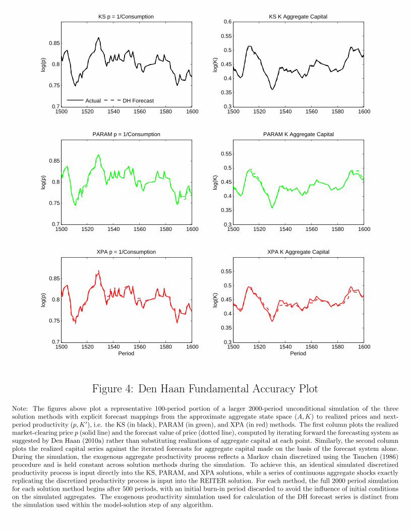
1500 1520 1540 1560 1580 16000.7

0.75

0.8

0.85

KS p = 1/Consumption

log(

p)

Actual DH Forecast

1500 1520 1540 1560 1580 16000.3

0.35

0.4

0.45

0.5

0.55

0.6KS K Aggregate Capital

log(

K)

1500 1520 1540 1560 1580 16000.7

0.75

0.8

0.85

PARAM p = 1/Consumption

log(

p)

1500 1520 1540 1560 1580 16000.3

0.35

0.4

0.45

0.5

0.55

PARAM K Aggregate Capital

log(

K)

1500 1520 1540 1560 1580 16000.7

0.75

0.8

0.85

XPA p = 1/Consumption

Period

log(

p)

1500 1520 1540 1560 1580 16000.3

0.35

0.4

0.45

0.5

0.55

XPA K Aggregate Capital

Period

log(

K)

Student Version of MATLABFigure 4: Den Haan Fundamental Accuracy Plot

Note: The figures above plot a representative 100-period portion of a larger 2000-period unconditional simulation of the threesolution methods with explicit forecast mappings from the approximate aggregate state space (A,K) to realized prices and next-period productivity (p,K ′), i.e. the KS (in black), PARAM (in green), and XPA (in red) methods. The first column plots the realizedmarket-clearing price p (solid line) and the forecast value of price (dotted line), computed by iterating forward the forecasting system assuggested by Den Haan (2010a) rather than substituting realizations of aggregate capital at each point. Similarly, the second columnplots the realized capital series against the iterated forecasts for aggregate capital made on the basis of the forecast system alone.During the simulation, the exogenous aggregate productivity process reflects a Markov chain discretized using the Tauchen (1986)procedure and is held constant across solution methods during the simulation. To achieve this, an identical simulated discretizedproductivity process is input directly into the KS, PARAM, and XPA solutions, while a series of continuous aggregate shocks exactlyreplicating the discretized productivity process is input into the REITER solution. For each method, the full 2000 period simulationfor each solution method begins after 500 periods, with an initial burn-in period discarded to avoid the influence of initial conditionson the simulated aggregates. The exogenous productivity simulation used for calculation of the DH forecast series is distinct fromthe simulation used within the model-solution step of any algorithm.

1 5 10 15 20−3

−2

−1

0

1

2

3Output

% R

espo

nse

REITER−EXTENDED

1 5 10 15 20−15

−10

−5

0

5

10

15Investment

% R

espo

nse

1 5 10 15 20−3

−2

−1

0

1

2

3Labor

% R

espo

nse

1 5 10 15 20−3

−2

−1

0

1

2

3Exogenous Productivity

% R

espo

nse

1 5 10 15 20−3

−2

−1

0

1

2

3p = 1/Consumption

% R

espo

nse

1 5 10 15 20−3

−2

−1

0

1

2

3Exogenous Demand

Period

% R

espo

nse

1 5 10 15 20−3

−2

−1

0

1

2

3Exogenous Labor Disutility

Period

% R

espo

nse

Student Version of MATLABFigure 5: Impulse Response, Demand Shock in Extended Model

Note: The figure above plots the linearized impulse response function to a positive shock to the aggregate demand series Dt in theextension of the heterogeneous firms model augmented with aggregate demand and labor preference shocks. These impulse responsesare computed after solving the extended model using the REITER technique and are therefore labelled REITER-EXTENDED. Giventhe endogenous variables Xt of the linearized system describing the economy, a solution Xt −XSS = A(Xt−1 −XSS) + Bεt of themodel trivially yields impulse responses At−1B representing the economy’s local response to each aggregate shock in the vector εt.The impulse response here is scaled by the assumed standard deviation of innovations to the aggregate demand series, with theexogenous shocked series itself plotted in the right hand side of the third row.

A Solution Methods

This section describes the equilibrium of the model with no aggregate uncertainty, as well as the detailsof the KS, PARAM, XPA, and REITER solution methods. To maintain generality, the bulk of the sectionfocuses on describing the algorithms or equilibrium concepts themselves. Therefore, some practical numericalissues involved in the solution techniques are mentioned in passing, but most numerical details (on grid sizes,optimization algorithms, etc) are deferred to a listing in Appendix B.

A.1 No Aggregate Uncertainty Model

The equilibrium definition of the steady-state model or model with no aggregate uncertainty is identical to theequilibrium with aggregate uncertainty discussed in the main text with constant aggregate productivity A.Unless otherwise specified, the steady-state model will be solved with A = 1. With a constant aggregate statespace, individual firm states are given by the far smaller state space (z, k), and solution of the no aggregateuncertainty model simply involves repeatedly guessing values of the market-clearing price or consumption,computing an ergodic cross-sectional distribution µ(z, k) based on the price-implied policies and adjustmentthresholds, and then checking consistency with the guessed price level. In the code available for this paper,the price clearing is performed using bisection, and calculation of an ergodic cross-sectional distributiongiven a price level follows the nonstochastic or histogram-based approach of Young (2010). In turn, thisapproach requires a projection grid for value functions, a denser simulation grid for idiosyncratic capital,and a discretized productivity process at the idiosyncratic level. For completeness, the equilibrium equationsare listed below:

V A(z, k) = maxk′,n

{p

(Azkαnν − k′ + (1− δ)k − φ

pn

)+ βEz′V (z′, k′)

}V NA(z, k) = max

n

{p

(Azkαnν − φ

pn

)+ βEz′V (z′, (1− δ)k)

}

V (z, k) = −φ∫ ξ∗(z,k)

0

ξdG(ξ) +G(ξ∗(z, k))V A(z, k) + [1−G(ξ∗(z, k))]V NA(z, k)

ξ∗(z, k) =V A(z, k)− V NA(z, k)

φ

1

p=

∫ ∫Azkαn(z, k, ξ)νdµ(z, k)dG(ξ)−

∫ ∫(k′(z, k, ξ)− (1− δ)k)dµ(z, k)dG(ξ),

where we have that policies for labor have a closed-form and capital policies follow a threshold rule,given optimal policies k

′∗(z, k) from V A(z, k):

k′(z, k, ξ) =

{k′∗(z, k), ξ ≤ ξ∗(z, k)

(1− δ)k, ξ > ξ∗(z, k),

and that µ(z, k) is the ergodic distribution implied by a discretization as in Young (2010) together withapplication of the capital policies, adjustment cost thresholds, and idiosyncratic productivity transitions.Once the equilibrium is obtained, it is trivial to compute aggregate capital as K =

∫kdµ(z, k).

A.2 Krusell Smith (KS)

The KS solution method used in the paper, following Khan and Thomas (2008) assumes that the set ofapproximating moments m in the aggregate state space of the model is equal to the mean or aggregatecapital level K. Further, the solution method discretizes idiosyncratic and aggregate productivity processesfollowing Tauchen (1986). Conditional upon a discretized level of aggregate productivity A, the forecastrules for price and next period’s aggregate capital level take a loglinear form:

log(p) = αp(A) + βp(A) log(K)

24

log(K ′) = αK(A) + βK(A) log(K).

Recall that from the household problem this yields a forecast wage level w = φp . Given these choices, the

solution algorithm works as follows. First, guess an initial forecast rule system Γ(1) = (α(1)p , β

(1)p , α

(1)K , β

(1)K ).

Then, before the solution iteration takes place, draw a large number T of exogenous aggregate productivityvalues based on the discretized Markov chain for A. Finally, in iteration s = 1, 2, ... do the following

1. Given forecast rule system Γ(s), solve the following system of equations via projection on some grid ofstates (z, k;A,K)

V A(s)(z, k;A,K) = maxk′,n

{p(s)(A,K)

(zAkαnν − k′ + (1− δ)k − w(s)(A,K)n

)+βEz′,A′V(s)(z

′, k′;A′, K ′(s))

}.

V NA(s) (z, k;A,K) = maxn

{p(s)(A,K)

(zAkαnν − w(s)(A,K)n

)+ βEz′,A′V(s)(z

′, (1− δ)k;A′, K ′(s))}

ξ∗(s)(z, k;A,K) =V A(s)(z, k;A,K)− V NA(s) (z, k;A,K)

φ,

V(s)(z, k;A,K) =−φ∫ ξ∗(s)(z,k;A,K)

0 ξdG(ξ) +G(ξ∗(s)(z, k;A,K)

)V A(s)(z, k;A,K)

+(

1−G(ξ∗(s)(z, k;A,K)

))V NA(s) (z, k;A,K)

which determines value function V(s)(z, k;A,K). Note that expectations are computed via summationover the appropriate portion of the discretized transition matrices Πz and ΠA for idiosyncratic andaggregate productivity, respectively, and that the solution to the Bellman equations can be achievedwith policy iteration, Howard acceleration of the Bellman equations, and continuous univariate op-timization techniques in next period’s capital level k′, such as Brent optimization or golden sectionsearch.

2. Given the value function solution from step 1, simulate the model. Simulation follows the nonstochasticapproach of Young (2010), and requires initialization of the cross-sectional distribution of capital andproductivity µ(z, k) over a dense, discrete grid of (zi, kj) with nd points for discretized capital. Ineach period t, market-clearing prices pt must be determined without reference to the forecast pricelevel p(s) (which appear only through embedded expectations in the continuation value). The priceclearing algorithm, for a given guessed price value p requires calculation of the excess demand or errorfunction, which is done as follows:

• Compute new capital and adjustment cutoff thresholds at each point on the dense simulationgrid (zi, kj) through

V A(zi, kj) = maxk′,n

{p(ziAk

αj n

ν − k′ + (1− δ)kj − φpn)

+βEz′,A′V(s)(z′, k′, ;A′, K ′(s))

}

V NA(zi, kj) = maxn

{p

(ziAk

αj n

ν − φ

pn

)+ βEz′,A′V(s)(z

′, (1− δ)kj , ;A′, K ′(s))}

ξ∗(zi, kj) =V A(zi, kj)− V NA(zi, kj)

φ

where the optimization over labor is a static problem which yields an analytical reduced-formfor the right hand side expressions which can be optimized in capital k′ alone. Let optimal laborand capital policies conditional upon adjustment be given by n∗(zi, kj) and k

′∗(zi, kj). We havesuppressed dependence on the aggregate states (A,K) for the moment, which is constant throughthe market-clearing process.

25

• Compute implied output, investment, consumption, and labor from

Y =∑zi,kj

µt(zi, kj)y(zi, kj), y(zi, kj) = ziAkαj n∗(zi, kj)

ν

I =∑zi,kj

µt(zi, kj)[G(ξ∗(zi, kj))(k

′∗(zi, kj)− (1− δ)kj)]

C = Y − I

N =∑zi,kj

µt(zi, kj)

(n∗(zi, kj) +

∫ ξ∗(zi,kj)

0

ξdG(ξ)

)

• Define the excess demand function or clearing error as 1p − C

• If excess demand is suitably small, the clearing algorithm stops. If not, repeat with an updatedvalue of p, using any preferred method such as bisection.

• With market clearing price pt in hand (as well as Yt, It, Ct, Nt), update the discretized distributionµt+1(zi, kj) for the next period. Based on Young (2010), distributional transitions are calculatedthrough linear interpolation of capital policies and use of the idiosyncratic productivity transitionmatrix

µt+1(zi′ , kj′) =∑zi

∑kj

Πzii′µt(zi, kj)

[ωa(i, j, j′)I(k′∗(zi, kj) ∈ [kj′−1, kj′+1])

+ωna(i, j, j′)I(kj ∈ [kj′−1, kj′+1])

]

ωa(i, j, j′) =

G (ξ∗(zi, kj))

(k′∗(zi,kj)−kj′kj′+1−kj′

)k′∗(zi, kj) ∈ [kj′ , kj′+1], 1 < j′ < nd

G (ξ∗(zi, kj)) k′∗(zi, kj) ≥ knd , j′ = nd

G (ξ∗(zi, kj)) k′∗(zi, kj) ≤ k1, j

′ = 1

ωna(i, j, j′) =

[1−G (ξ∗(zi, kj))]

(kj−kj′−1

kj′−kj′−1

)kj ∈ [kj′−1, kj′ ], 1 < j′ < nd

[1−G (ξ∗(zi, kj))] kj ≥ knd , j′ = nd[1−G (ξ∗(zi, kj))] kj ≤ k1, j

′ = 1

where above kj = max((1− δ)kj , k1) is the non-adjustment next-period capital stock. Also, withµt+1 in hand, next period’s simulated capital stock is computable as

Kt+1 =∑zi,kj

µt+1(zi, kj)kj .

• Continue to simulate period t+ 1.

3. With the simulation from periods 1 to T completed given forecast rules Γ(s), discard some number Tergof periods as initialization, and update the forecast rules based on OLS regressions. Run the loglinearOLS regressions of realized prices pt on aggregate capital stocks Kt and realized next-period capitalstocks Kt+1 on current stocks Kt, where new coefficients (αp, βp, αK , βK) are obtained separatelyfor each level of aggregate productivity, and compute forecast rule errors as the maximum absolutedifference between assumed coefficients Γ(s) and the new estimated values. If the coefficients have

converged to an acceptable tolerance, the model is solved. If not, then update Γ(s+1) using dampened

fixed-point iteration (i.e. set Γ(s+1) equal to a weighted average of Γ(s) and the newly estimatedcoefficients), then continue to solution iteration s+ 1.

26

A.3 Parametrized Distributions (PARAM)

This is a discussion of the computational algorithm due to Algan et al. (2008, 2010a) (henceforth AADH)which relies upon higher-order reference moments, as well as assumed functional forms for the cross-sectionaldistribution of idiosyncratic capital and productivity µ(z, k) in the solution of the model.

Just as in the KS algorithm, we first must discretize the aggregate and idiosyncratic productivity pro-cesses following Tauchen (1986). Let the number of idiosyncratic (aggregate) productivity points be givenby nz(nA). Then, prior to the solution of the model, we first determine a set of aggregate moments m to beincluded in the aggregate state space. Here, this will be the singleton of aggregate capital, the cross-sectionalmean K. Together with aggregate productivity, (A,K) therefore forms the aggregate state. Then, deter-mine a set of reference moments mref used to help pin down the shape of the cross-sectional distributionof idiosyncratic capital and productivity. Here, this will be the first nMnz centered moments of the capitaldistribution conditional upon each value of idiosyncratic productivity. Also, compute the exogenous ergodicdistribution of idiosyncratic productivity πz for future use.

The reference moments are needed in this algorithm because, together with the aggregate capital state,they jointly determine the coefficients of the flexible exponential function form for the approximation toµ(zi, k) at discretized levels of zi:

P (k, ρzi) = ρzi0 exp

{ρzi1 (k −mzi

1 ) + ρzi2[(k −mzi

1 )2 −mzi2

]+...+ ρzinM

[(k −mzi

1 )nM −mzinM

] }.

As discussed in AADH, a well-behaved convex minimization problem which is laid out below yieldsa mapping between the nznM moments of the cross-sectional distribution and coefficient vectors ρzi , i =1, ..., nz, because the first-order conditions of this problem are identical to the moment conditions settingdistributional and reference moments equal to each other. We assume when manipulating or integrating thisdistribution that idiosyncratic capital lies in the bounds [k, k].

To solve the model, start with an initial constant guess for these reference moments, from the distributionin the steady-state model with no aggregate uncertainty. If desired, simulation can later provide a setof reference moments which vary with the level of aggregate productivity, or these steady-state referencemoments themselves can be held fixed. Although we will outline both the repeated simulation and simulation-free approaches below, the results reported in the paper hold the reference moments at their steady-statelevels. Finally, another option is also to use a regression forecast system from (A,K) → mref , althoughfollowing AADH we forego that approach here.

1. Iterate over the reference moments or the reference moment forecasting system, which yields a constantor variable mapping (A,K)→ mref .

(a) Loop over the aggregate states (A,K), on the discretized grid for A and some projection grid forK.

• For each (A,K) and implied mref (A,K), choose distributional coefficientsρziA,K,1, ..., ρ

ziA,K,nM

, i = 1, ..., nz to solve

minρziA,K ,i=1,...,nz

nz∑i=1

∫ k

k

P (k, ρziA,K)dk,

noting that the constants ρzia,K,0 are irrelevant for the minimization and are simply chosento ensure integration to 1. This is a well-behaved convex minimization problem and theintegral can be computed via any standard quadrature rule. Here and throughout, integralsare computed via Simpson’s rule. It is important to note that any rule with fixed nodesand weights is preferable to adaptive methods because fixed rules contribute to stabilityin the minimization problem above. The minimization is implemented in this paper usinga robust and quick quasi-Newton routine with symmetric rank-one (SR1) updating of theapproximation to the inverse Hessian.

(b) Iterate over V(s)(z, k; a,K) to convergence.

27

• Loop over the aggregate states (A,K). For each (A,K), use any nonlinear equation systemsolver in p,K ′ to obtain p(A,K) and K ′(A,K). The method used in this paper is dampenedfixed-point iteration in the pair p,K ′.

– For each value of p,K ′, evaluate on the discretized grid for z and some spline projectiongrid for k the following equations:

V A(s+1)(z, k;A,K) = maxk′,n

{p(zAkαnν − k′ + (1− δ)k − φ

pn)

+βEz′,A′V(s)(z′, k′;A′,K ′)

}

V NA(s+1)(z, k;A,K) = maxn

{p

(zAkαnν − φ

pn

)+ βEz′,A′V(s)(z

′, (1− δ)k;A′,K ′)

}

ξ∗(z, k;A,K) =V A(s+1)(z, k;A,K)− V NA(s+1)(z, k;A,K)

φ

V(s+1)(z, k;A,K) =−φ∫ ξ∗(z,k;A,K)

0ξdG(ξ) +G(ξ∗(z, k;A,K))V A(s+1)(z, k;A,K)

+ (1−G(ξ∗(z, k;A,K)))V NA(s+1)(z, k;A,K)

– Then, compute the errors to the system of equations in p and K ′ given by

1

p=

nz∑i=1

πzi

∫ k

k

[zAkαn(zi, k;A,K)ν

−G(ξ∗(zi, k;A,K))(k′(zi, k;A,K)− (1− δ)k)

]P (k, ρziA,K)dk

K ′ =

nz∑i=1

πzi

∫ k

k

[G(ξ∗(zi, k;A,K))k′(zi, k;A,K)

+(1−G(ξ∗(zi, k;A,K)))(1− δ)k

]P (k, ρziA,K)dk,

where above the calculation requires the ability to compute n(zi, k;A,K), k′(zi, k;A,K),and ξ∗(zi, k;A,K) at a set of Simpson integration nodes in k. These can be computed byrecalculation of the right hand sides of the Bellman equations above at the quadraturenodes in k, and this task is simplified by noting that capital policies depend only onidiosyncratic productivity and that the labor demand optimization is static and canbe obtained in closed-form. Also, the densities P (k, ρziA,K) must be evaluated usingmoments which reflect both the reference moments for higher order terms but also thecurrent mean level of aggregate capital. Therefore, the first moments of capital used inthe construction of P (k, ρziA,K) are linearly shifted to deliver consistency with K as thecurrent aggregate shape.

• Error on the value function iteration is given by ||V(s+1) − V(s)||, which can be defined asdesired. The solution used in this paper is based on the max absolute percentage difference.If the value function has converged, exit the value function iteration process. If not, goiteration s+ 1.

(c) At this point, a decision must be made. If the reference moments used in the solution are to beheld fixed at their steady-state values, the model is now solved. However, if the reference momentsare to be updated with simulation, then simulation must be performed as part of the solutionitself. In either case, simulation proceeds as follows, noting that a set of exogenous productivitydraws At for T periods have been made outside of the solution loop. Given converged valuesV , simulate the economy for a large number of periods, in each period imposing market clearingto obtain p,K ′. For each period, do the following, taking advantage of the functional formsassumed for the cross-sectional density.

• Start period t with a set of coefficients ρzit and moments mt (the first nznM moments of theidiosyncratic capital density conditional upon idiosyncratic productivity) which jointly pindown the cross-sectional density in (z,K) for the period. Then using the value function fromabove and the same fixed point iteration approach, compute the equilibrium p,K ′ consistentwith both the value function and the cross-sectional distributions for the current period.

28

• Compute the value of all reference moments for the next period t + 1. These are higher-order centered moments of the cross-sectional distribution of capital next period, and canbe computed directly via quadrature, given the policies and cross-sectional distributioncoefficients of period t.

• Now that the reference moments are set for period t + 1, along with the aggregate capitalstate, compute the coefficients of the cross-sectional distribution associated with period t+1using the exact same minimization step as above.

(d) After simulation is completed for all T periods, and a certain number Terg of initial periods arediscarded, you have two options. If the reference moments are held constant at their steady-state values, you simply have an unconditional simulation of the model. If a fixed-point on thereference moments is desired, then update the reference moments in the outer loop now. The ap-propriate method depends on your assumptions for the reference moments. If you have assumedone unconditional constant set of reference moments not varying with aggregates, compute theunconditional average of each reference moment over the simulation. If you have assumed refer-ence moments which vary with aggregate productivity, then compute the conditional average ofeach reference moment on the value of aggregate productivity. If you have assumed a referencemoment forecasting system, update this system with OLS. Return to step (a) if the referencemoments have not converged based on some criterion, say max absolute difference.

A.4 Explicit Aggregation (XPA)

First discretize the aggregate productivity process A and solve the steady-state model for each aggregateproductivity value Ak, k = 1, ..., nA. For each level, save values of equilibrium price and capital stockspSS(Ak),KSS(Ak). Also, discretize the idiosyncratic productivity process and store the exogenous ergodicdistribution πz of discretized idiosyncratic productivity for future use.

Set up the aggregate state space to include (A,K) and posit forecast rules for market-clearing pricesand next-period capital identical to the KS case. Then, solve the model exactly as in the case of the KSalgorithm, with two modifications:

(2’) Replace KS simulation step (2) with an “explicit aggregation” step. In particular, loop over aggregatestates (A,K), where A varies over its discretized grid and K varies over the same projection grid usedto compute the value functions.

• At each point (A,K), compute market-clearing prices via a solution routine like bisection overprice p, with implied output, investment, consumption, and next-period aggregate capital givena guess p defined by

Y =∑zi

πiy(zi,K), y(zi,K) = ziAKαn∗(zi,K)ν

I =∑zi

πi

[G(ξ∗(zi,K))(k

′∗(zi,K)− (1− δ)K)]

C = Y − I

K ′ =∑zi

πi

[G(ξ∗(zi,K))k

′∗(zi,K) + (1− [G(ξ∗(zi,K)))(1− δ)K)]

with clearing error given as before by 1p − C.

• Note that the end of this iteration generates a dataset (A,K) → (p,K ′) as (A,K) varies overthe discretization and projection grids.

(3’) Replace KS update step (3) with a forecast update rule step using the dataset defined by explicitaggregation step (2’).

29

• First, update the current vector of forecast rule coefficients Γ(s) by estimating

(αp(A), βp(A), αK(A), βK(A)) with OLS on the explicit aggregation dataset, segmented by dis-cretized value of A.

• Then, define a vector of nA bias correction terms

xBiasp (A) = αp(A) + βp(A) log(KSS(A))− log(pSS(A))

xBiasK (A) = αK(A) + βK(A) log(KSS(A))− log(KSS(A))

and adjust the new forecast rule coefficients’ constant terms with

αp(A)← αp(A)− xBiasp (A)

αK(A)← αK(A)− xBiasK (A).

• Then, check the estimated coefficients against the old coefficients Γ(s). If they are within sometolerance according to max absolute deviations, the model is solved and exit the routine. If theforecast rules have not converged, use dampened fixed-point iteration to update the forecast rulesystem Γ(s+1) based on rule (s) and the newly estimated system.

Note that the differencing off of xBias(A) is an attempt to correct for the Jensen’s inequality bias inducedby substitution of aggregate states into idiosyncratic policies. The bias results from lack of variation in thecross-section of idiosyncratic capital when recovering market-clearing prices and next-period capital stocks.However, the steady-state model prices and capital stocks do incorporate cross-sectional integration over adistribution of idiosyncratic capital presumably similar to the distributions within the model with aggregateuncertainty. The modification by the term xBias(A) requires that the estimated forecast system be able toexactly reproduce as a fixed point the steady-state prices and aggregate capital stocks pSS(A) and KSS(A),conditional upon aggregate productivity.

Note also that after the model is solved, simulation is completed exactly as in the KS algorithm, usingthe Young (2010) nonstochastic or histogram-based approach, and requiring market-clearing in each periodwith integration over the full cross-sectional distribution of idiosyncratic capital.

A.5 Projection Plus Perturbation (REITER)

The REITER solution method is based on three steps, and provides a perturbation approximation to thefull rational expectations equilibrium. The first step is to solve the steady-state version of the model, withno aggregate uncertainty and aggregate productivity held fixed at a value of A = 1. The steady-statesolution is identical to the one used, for example, as an input into the PARAM solution. The second stepis to set up a system of nonlinear equations defining the model’s equilibrium, which is covered in the firstsubsection below. The final step is to linearize and solve the system using standard numerical differentiationand solution techniques, covered in the second subsection below.

A.5.1 Nonlinear System of Equations in the Discretized Model

We first establish a grid of nz idiosyncratic productivity points and a Markov transition matrix Πzij =P(zt+1 = zj |zt = zi) following Tauchen (1986). Then, we establish a grid of nk idiosyncratic capital stocknodes ki, which will function as knot points for cubic spline interpolation of the value functions. Finally, adenser simulation grid of nd idiosyncratic points will be used to store the distribution. We then have thefollowing equations, which are to be linearized around the zero-aggregate uncertainty steady-state of themodel.

V At−1(zi, kj) = maxk′

pt−1 (f(At−1, zi, kj , wt−1)− k′ + (1− δ)kj) + β∑zi′

Πzii′Vt(zi′ , k′)

+ ηAt,i,j

30

f(At−1, zi, kj , wt−1) = (1− ν)

(ν

wt−1

) ν1−ν

(At−1zi)1

1−ν kα

1−νj

V NAt−1 (zi, kj) = pt−1f(At−1, zi, kj , wt−1) + β∑zi′

Πzii′Vt(zi′ , kj) + ηNAt,i,j

kj = max((1− δ)kj , k1)

Vt−1(zi, kj) = −φ∫ ξ∗t−1(zi,kj)

0ξdG(ξ) +G

(ξ∗t−1(zi, kj)

)V At−1(zi, kj)

+[1−G

(ξ∗t−1(zi, kj)

)]V NAt−1 (zi, kj)

ξ∗t−1(zi, kj) =V At−1(zi, kj)− V NAt−1 (zi, kj)

φ

µt(zi′ , kj′) =∑zi

∑kj

Πzii′µt−1(zi, kj)

[ωa(i, j, j′)I(k′(zi, kj) ∈ [kj′−1, kj′+1])

+ωna(i, j, j′)I(kj ∈ [kj′−1, kj′+1])

]

ωa(i, j, j′) =

G(ξ∗t−1(zi, kj)

) (k′(zi,kj)−kj′kj′+1−kj′

)k′(zi, kj) ∈ [kj′ , kj′+1], 1 < j′ < nd

G(ξ∗t−1(zi, kj)

)k′(zi, kj) ≥ knd , j′ = nd

G(ξ∗t−1(zi, kj)

)k′(zi, kj) ≤ k1, j

′ = 1

ωna(i, j, j′) =

[1−G

(ξ∗t−1(zi, kj)

)] ( kj−kj′−1

kj′−kj′−1

)kj ∈ [kj′−1, kj′ ], 1 < j′ < nd[

1−G(ξ∗t−1(zi, kj)

)]kj ≥ knd , j′ = nd[

1−G(ξ∗t−1(zi, kj)

)]kj ≤ k1, j

′ = 1

1

pt−1=∑zi

∑kj

µt−1(zi, kj)[y(At−1, zi, kj , wt−1)−G

(ξ∗t−1(zi, kj)

)(k′(zi, kj)− (1− δ)kj)

]wt−1 =

φ

pt−1

Yt−1 =∑zi

∑kj

µt−1(zi, kj)y(At−1, zi, kj , wt−1)

y(At−1, zi, kj , wt−1) =

(ν

wt−1

) ν1−ν

(At−1zi)1

1−ν kα

1−νj

It−1 =∑zi

∑kj

µt−1(zi, kj)G(ξ∗t−1(zi, kj)

)(k′(zi, kj)− (1− δ)kj)

Nt−1 =∑zi

∑kj

µt−1(zi, kj)

[n(At−1, zi, kj , wt−1) +

∫ ξ∗t−1(zi,kj)

0

ξdG(ξ)

]

n(At−1, zi, kj , wt−1) =

(ν

wt−1

) 11−ν

(At−1zi)1

1−ν kα

1−νj

log(At) = ρA log(At−1) + εt, εt ∼iid N(0, σ2A)

Together, the above system represents a total of ns = 3nznk +nznd + 5 equations in the ns× 1 vector ofendogenous variables Xt =

((V At )′, (V NAt )′, V ′t , µ

′t, log(pt), log(Yt), log(It), log(Nt), log(At)

)′, together with

the exogenous shock process εt. We write this nonlinear rational expectations system corresponding to thediscretized model as F (Xt, Xt−1, ηt, εt) = 0, where F (·) is the left hand side minus the right hand side ofeach of the ns equations above. Note that we know this equation is satisfied exactly at the steady-statevalue of Xt = Xt−1 = XSS and ηt = 0, εt = 0 corresponding to no aggregate uncertainty and At = 1. Thevectors Xt are ns × 1 while the vector ηt is nη × 1, where nη = 2nznk.

31

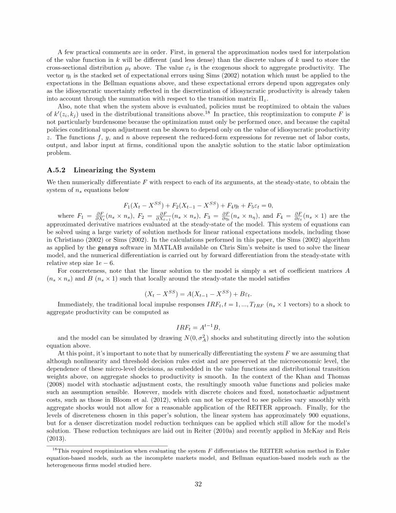
A few practical comments are in order. First, in general the approximation nodes used for interpolationof the value function in k will be different (and less dense) than the discrete values of k used to store thecross-sectional distribution µt above. The value εt is the exogenous shock to aggregate productivity. Thevector ηt is the stacked set of expectational errors using Sims (2002) notation which must be applied to theexpectations in the Bellman equations above, and these expectational errors depend upon aggregates onlyas the idiosyncratic uncertainty reflected in the discretization of idiosyncratic productivity is already takeninto account through the summation with respect to the transition matrix Πz.

Also, note that when the system above is evaluated, policies must be reoptimized to obtain the valuesof k′(zi, kj) used in the distributional transitions above.18 In practice, this reoptimization to compute F isnot particularly burdensome because the optimization must only be performed once, and because the capitalpolicies conditional upon adjustment can be shown to depend only on the value of idiosyncratic productivityz. The functions f , y, and n above represent the reduced-form expressions for revenue net of labor costs,output, and labor input at firms, conditional upon the analytic solution to the static labor optimizationproblem.

A.5.2 Linearizing the System

We then numerically differentiate F with respect to each of its arguments, at the steady-state, to obtain thesystem of ns equations below

F1(Xt −XSS) + F2(Xt−1 −XSS) + F4ηt + F5εt = 0,

where F1 = ∂F∂Xt

(ns × ns), F2 = ∂F∂Xt−1

(ns × ns), F3 = ∂F∂ηt

(ns × nη), and F4 = ∂F∂εt

(ns × 1) are the

approximated derivative matrices evaluated at the steady-state of the model. This system of equations canbe solved using a large variety of solution methods for linear rational expectations models, including thosein Christiano (2002) or Sims (2002). In the calculations performed in this paper, the Sims (2002) algorithmas applied by the gensys software in MATLAB available on Chris Sim’s website is used to solve the linearmodel, and the numerical differentiation is carried out by forward differentiation from the steady-state withrelative step size 1e− 6.

For concreteness, note that the linear solution to the model is simply a set of coefficient matrices A(ns × ns) and B (ns × 1) such that locally around the steady-state the model satisfies

(Xt −XSS) = A(Xt−1 −XSS) +Bεt.

Immediately, the traditional local impulse responses IRFt, t = 1, ..., TIRF (ns × 1 vectors) to a shock toaggregate productivity can be computed as

IRFt = At−1B,

and the model can be simulated by drawing N(0, σ2A) shocks and substituting directly into the solution

equation above.At this point, it’s important to note that by numerically differentiating the system F we are assuming that

although nonlinearity and threshold decision rules exist and are preserved at the microeconomic level, thedependence of these micro-level decisions, as embedded in the value functions and distributional transitionweights above, on aggregate shocks to productivity is smooth. In the context of the Khan and Thomas(2008) model with stochastic adjustment costs, the resultingly smooth value functions and policies makesuch an assumption sensible. However, models with discrete choices and fixed, nonstochastic adjustmentcosts, such as those in Bloom et al. (2012), which can not be expected to see policies vary smoothly withaggregate shocks would not allow for a reasonable application of the REITER approach. Finally, for thelevels of discreteness chosen in this paper’s solution, the linear system has approximately 900 equations,but for a denser discretization model reduction techniques can be applied which still allow for the model’ssolution. These reduction techniques are laid out in Reiter (2010a) and recently applied in McKay and Reis(2013).

18This required reoptimization when evaluating the system F differentiates the REITER solution method in Eulerequation-based models, such as the incomplete markets model, and Bellman equation-based models such as theheterogeneous firms model studied here.

32

B General Numerical Choices and Additional Accuracy Statistics

To complement the general discussion of each solution algorithm, it is also useful to list some practical choicesmade in the projection, optimization, and discretization of the model, with further information available inTable B1.

Table B1: Some Choices for the Numerical Solutions

Object Value Type or Location Usedk nodes for V spline interpolation 10 Loglinear [0.1,8.0]k points for KS, XPA distribution histogram 50 Loglinear [0.1,8.0]k points for REITER distribution histogram 150 Loglinear [0.1,8.0]K points for V linear interpolation 10 Linear [1.25,2.0]A points in discretization 5 Loglinear [0.94,1.0562]z points in discretization 5 Loglinear [0.9176,1.0897]V or k′, ξ∗ tolerance 0.0001 All methodsForecast rule coefficient tolerance 0.001 KS, XPA methodsHoward accelerations 50 All methods but PARAMNumber of reference moments 4 PARAM method densitiesQuadrature nodes in k 36 PARAM method integrationNondiscarded simulation periods T − Terg 2000 All methodsNumber of IRF simulations 2000 All methodsIRF simulations length 50 All methodsIRF shock period 25 All methods

Note: The table above indicates specific methods, tolerances, grid sizes and densities, and simulation lengths usedin the numerical implementation of the solution techniques discussed in the paper. The code used to produce theresults in this paper is available on Stephen Terry’s website.

• The mean or aggregate level of capital K is used as the approximating moment m for the cross-sectional distribution µ(z, k) for the three solution methods requiring such an approximation (KS,PARAM, and XPA).

• In all solution techniques, idiosyncratic and aggregate productivity processes z and A are discretizedaccording to Tauchen (1986) and along grids spanning two standard deviations of the unconditionalprocess standard deviation around the process steady-state.19

• Value functions are approximated as cubic splines in idiosyncratic capital k with a natural splineendpoint condition, and using linear interpolation in aggregate capital K. For the KS, XPA, andno-aggregate uncertainty models, the firm problem is solved using policy iteration with Howard accel-eration of the value function, while in the PARAM method value function iteration is performed.

• The idiosyncratic capital policies within the Bellman equations are determined using Brent opti-mization (KS, XPA, PARAM, and no aggregate uncertainty), or golden section search (REITERdifferentiation).

• Price-clearing is performed during simulation using bisection (XPA, no aggregate uncertainty) orhybrid bisection/inverse quadratic interpolation (KS). Within the model solution step, joint searchfor clearing price and next period aggregate capital is performed using dampened fixed point iteration(PARAM).

• Minimization of the density-based objective determining distributional coefficients during simulationand solution of the PARAM model is performed using a standard quasi-Newton algorithm with sym-metric rank-one (SR1) updates to the inverse Hessian approximation.

19For the REITER method, the aggregate productivity process A must take on continuous values within the solutionprocess, but when simulating we use both the discretized process as well as separately consider the continuouslysimulated shocks.

33

• Within the PARAM solution, integration over the cross-sectional densities is performed using standardSimpson quadrature rules.

Table B2: Additional Accuracy Statistics for Forecast Rules

Statistic K ′, KS K ′, XPA K ′, PARAM p, KS p, XPA, p, PARAMRMSE, A = A1 0.0182 0.5506 0.1257 0.0122 0.8911 0.0501RMSE, A = A2 0.0337 0.2081 0.0903 0.0247 0.1832 0.0607RMSE, A = A3 0.0486 0.3535 0.1007 0.0430 0.1230 0.0663RMSE, A = A4 0.0613 0.3804 0.1899 0.0604 0.2732 0.1211RMSE, A = A5 0.0792 0.4256 0.3090 0.0883 0.7054 0.2010

R2, A = A1 0.9999 0.9350 0.9973 0.9999 -0.1915 0.9977R2, A = A2 0.9999 0.9910 0.9988 0.9997 0.9777 0.9981R2, A = A3 0.9998 0.9670 0.9981 0.9993 0.9916 0.9977R2, A = A4 0.9996 0.9604 0.9912 0.9984 0.9468 0.9910R2, A = A5 0.9992 0.9575 0.9692 0.9959 0.3850 0.9696

Note: The table above reports internal accuracy statistics based on unconditional simulations for the three solutionmethods with explicit forecast mappings from the approximate aggregate state (A,K) to realized next-period capitalK′ (the first three columns) and to market-clearing prices p (the final three columns). The first five rows representthe root mean squared error, in 100 times logs, between the forecasts of one-period ahead capital and current priceand realized values, conditional upon the current discretized value of aggregate productivity A1, ..., A5. The final fiverows represent the R2 of each forecast regression, conditional upon the current value of aggregate productivity. Theexogenous aggregate productivity process reflects a Markov chain discretized using the Tauchen (1986) procedure andis held constant across solution methods during the simulation. To achieve this, an identical simulated discretizedproductivity process is input directly into the KS, PARAM, and XPA solutions, while a series of continuous aggregateshocks exactly replicating the discretized productivity process is input into the REITER solution. For each method,the full 2000 period simulation for each solution method begins after 500 periods, with an initial burn-in perioddiscarded to avoid the influence of initial conditions on the simulated aggregates. The exogenous productivitysimulation used for calculation of the accuracy statistics are distinct from the simulation used within the model-solution step of any algorithm.

C Simulated Impulse Responses with Nonlinear Models

As noted in the main text, nonlinear impulse response analysis must take into account variation in the initialconditions and size of the imposed shocks, and following Koop et al. (1996) we take the following approachto compute the average conditional response to a one-standard deviation aggregate productivity shock:

1. Fix a large number N of simulations, a per-simulation length TIRF , and a shock-period Tshock.

2. Independently draw exogenous uit ∼ U(0, 1) shocks for each period t of each simulation i, as well asone “shock occurrence” si ∼ U(0, 1) draw for each simulation i.

3. For each simulation i, based on comparison of the shocks uit with the entries of the cumulated transitionmatrix of discretized aggregate productivity, create two versions of simulated aggregate productivityseries Ashockit and Anoshocksit , which are identical until the shock-period for t < Tshock. In the shockperiod Tshock for each simulation, compare the shock occurrence draw si for simulation i with thecutoff thresholds s defined below. If si ≤ s, set AshockiTshock

= AnA, where nA is the highest level of the

discretized aggregate productivity process, and then allow Ashockit to transit normally based on uit fort > Tshock. If si > s, allow Ashockit to transit normally based on uit for all periods t ≥ Tshock. In eithercase, allow Anoshocksit to transit normally based on uit for all t ≥ Tshock.

4. Simulate any aggregate series of interest X twice, using both Ashockit and Anoshockit exogenous processes.The impulse responses xt of series X in period t to an aggregate productivity shock in period Tshockis given by

xt = 1001

N

N∑i=1

log

(Xshockit

Xnoshockit

).

34

To obtain an average percentage innovation in aggregate productivity which equals σA exactly, we choosethe shock threshold s to solve

σA = s

nA∑k=1

πAk (log(AnA)− log(Ak)) ,

where πA is the ergodic distribution of the discretized aggregate productivity process A.As noted in Appendix B, to compute the impulse responses plotted in the main text, we set TIRF = 50,

Tshock = 25, and N = 2000, and we hold exogenous draws uit, si constant across simulation methods. Wealso set nA = 5.

One final comment is in order regarding the REITER solution method. Because the REITER approachyields a linearized solution, the simulation-based analysis of Koop et al. (1996) is unnecessary. Althoughfor completeness and comparability we perform the simulation-based impulse response with the REITERmethod, a much simpler alternative, invariant to shock scaling or initial conditions, is available. In particular,when writing the REITER solution as Xt = AXt−1 + BεAt, where Xt is the endogenous vector defined inAppendix A and εAt is a continuous shock to aggregate productivity εAt ∼ N(0, σ2

A), the linear impulseresponse is given by

xREITER−LINt = At−1B,

which is a vector of responses of each endogenous variable to an innovation in εAt. Figure C1 plots thesimulated impulse response and the linearized version immediately computable from the solution matrices,unsurprisingly confirming that they are virtually identical.

D Adding Aggregate Complexity with the REITER Method

To add a persistent demand or preference shock Dt as well as a labor disutility process DNt to the baseline

heterogeneous firms context considered here, replace the household objective based on maximization of

E0

∞∑t=0

βtU(Ct, 1−Nt)

with maximization of the alternative

E0

∞∑t=0

βtDtU∗(Ct, Nt, D

Nt ),

U∗(Ct, Nt, DNt ) = log(Ct)− φDN

t Nt

log(Dt) = ρD log(Dt−1) + σDεDt

log(DNt ) = ρN log(DN

t−1) + σNεNt .

First order conditions for the modified problem immediately reveal that firms owned by householdssubject to the shocks Dt and DN

t will value dividend flows at the rate ptDt where pt = 1Ct

, and equilibrium

wages are given by wt =φDNtpt

. By replacing price pt and wage wt with the formulas above in the system

F from the REITER discussion of Appendix A, and adding the evolution equations for Dt and DNt , we

immediately obtain a system with two more endogenous variables and two more exogenous shock processes,which can be linearized and solved using numerical differentiation and the solution technique of Sims (2002),exactly as in the baseline REITER method.

The impulse responses from this model are computed using the somewhat arbitrary choices of ρD =ρN = 0.859, identical to the persistence of aggregate productivity, scaled by the standard deviations σD =σN = 0.014, also equal to baseline aggregate productivity volatility. The main text displays the response to ademand shock Dt, while Appendix Figures D1 and D2 plot local impulse responses to aggregate productivityand labor disutility shocks, respectively.

35

1500 1510 1520 1530 1540 1550 1560 1570 1580 1590 16000.7

0.72

0.74

0.76

0.78

0.8

0.82

0.84

0.86

0.88

Period

log(

p), p

= 1

/Con

sum

ptio

n

REITER Baseline REITER Higher Density

Student Version of MATLABFigure B1: REITER Price Dynamics, Baseline and Denser Discretization

Note: The figure above plots a representative 100-period portion of a larger 2000-period unconditional simulation of the marketclearing price series pt obtained by applying the REITER solution method with two histogram grid densities: 150 grid points (solidline) and 200 grid points (dotted line). For each method, the full 2000 period simulation for each solution method begins after 500periods, with an initial burn-in period discarded to avoid the influence of initial conditions on the simulated aggregates.

1500 1520 1540 1560 1580 16000.7

0.75

0.8

0.85

KS p = 1/Consumption

log(

p)

Actual Forecast

1500 1520 1540 1560 1580 16000.3

0.35

0.4

0.45

0.5

0.55

0.6KS K Aggregate Capital

log(

K)

1500 1520 1540 1560 1580 16000.7

0.75

0.8

0.85

PARAM p = 1/Consumption

log(

p)

1500 1520 1540 1560 1580 16000.3

0.35

0.4

0.45

0.5

0.55

PARAM K Aggregate Capital

log(

K)

1500 1520 1540 1560 1580 16000.7

0.75

0.8

0.85

XPA p = 1/Consumption

log(

p)

Period1500 1520 1540 1560 1580 1600

0.3

0.35

0.4

0.45

0.5

0.55

XPA K Aggregate Capital

log(

K)

Period

Student Version of MATLABFigure B2: Realizations vs. One-Period Ahead Forecasts

Note: The figures above plot a representative 100-period portion of a larger 2000-period unconditional simulation of the threesolution methods with explicit forecast mappings from the approximate aggregate state space (A,K) to realized prices and next-period productivity (p,K ′), i.e. the KS (in black), PARAM (in green), and XPA (in red) methods. The first column plots therealized market-clearing price p (solid line) and the forecast value of price (dotted line), given the currently realized value of (A,K).The second column plots the realized capital series (solid line) against the one-period ahead forecasts (dotted line) made on thebasis of (A,K). During the simulation, the exogenous aggregate productivity process reflects a Markov chain discretized using theTauchen (1986) procedure and is held constant across solution methods during the simulation. To achieve this, an identical simulateddiscretized productivity process is input directly into the KS, PARAM, and XPA solutions, while a series of continuous aggregateshocks exactly replicating the discretized productivity process is input into the REITER solution. For each method, the full 2000period simulation for each solution method begins after 500 periods, with an initial burn-in period discarded to avoid the influenceof initial conditions on the simulated aggregates.

1 5 10 15 20−3

−2

−1

0

1

2

3Output

% R

espo

nse

REITERREITER−LIN

1 5 10 15 20−15

−10

−5

0

5

10

15Investment

% R

espo

nse

1 5 10 15 20−3

−2

−1

0

1

2

3Labor

% R

espo

nse

1 5 10 15 20−3

−2

−1

0

1

2

3Exogenous Productivity

Period

% R

espo

nse

1 5 10 15 20−3

−2

−1

0

1

2

3p = 1/Consumption

Period

% R

espo

nse

Student Version of MATLABFigure C1: Impulse Response, Linear vs. Simulation-Based

Note: The figure above plots the linearized impulse response function (in dotted lines, labelled REITER-LIN) to a positive shockto the aggregate productivity series At in the baseline REITER solution of the heterogeneous firms model. Given the endogenousvariables Xt of the linearized system describing the economy, a solution Xt −XSS = A(Xt−1 −XSS) + BεAt of the model triviallyyields impulse responses At−1B representing the economy’s local response to the aggregate productivity shock εAt. The impulseresponse here is scaled by the assumed standard deviation of innovations to the aggregate productivity series, with the exogenousshocked series itself plotted in the right hand side of the second row. In solid lines labelled REITER, the figure plots analogous impulseresponses computed as suggested by Koop et al. (1996), based on 2000 repeated simulations of a discretized aggregate productivityprocess of 50-period length each, with and without imposed productivity shocks at the period labelled 1 above. The REITER-LINresponses should be interpreted as 100 times log deviations from steady-states, while the REITER responses are equal to 100 timesaverage log differences between the shocked and unshocked simulations.

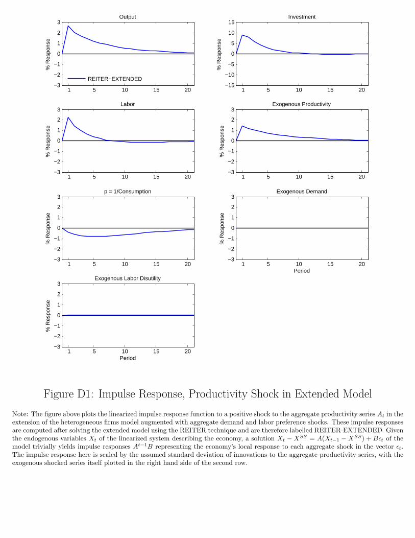
1 5 10 15 20−3

−2

−1

0

1

2

3Output

% R

espo

nse

REITER−EXTENDED

1 5 10 15 20−15

−10

−5

0

5

10

15Investment

% R

espo

nse

1 5 10 15 20−3

−2

−1

0

1

2

3Labor

% R

espo

nse

1 5 10 15 20−3

−2

−1

0

1

2

3Exogenous Productivity

% R

espo

nse

1 5 10 15 20−3

−2

−1

0

1

2

3p = 1/Consumption

% R

espo

nse

1 5 10 15 20−3

−2

−1

0

1

2

3Exogenous Demand

Period

% R

espo

nse

1 5 10 15 20−3

−2

−1

0

1

2

3Exogenous Labor Disutility

Period

% R

espo

nse

Student Version of MATLABFigure D1: Impulse Response, Productivity Shock in Extended Model

Note: The figure above plots the linearized impulse response function to a positive shock to the aggregate productivity series At in theextension of the heterogeneous firms model augmented with aggregate demand and labor preference shocks. These impulse responsesare computed after solving the extended model using the REITER technique and are therefore labelled REITER-EXTENDED. Giventhe endogenous variables Xt of the linearized system describing the economy, a solution Xt −XSS = A(Xt−1 −XSS) + Bεt of themodel trivially yields impulse responses At−1B representing the economy’s local response to each aggregate shock in the vector εt.The impulse response here is scaled by the assumed standard deviation of innovations to the aggregate productivity series, with theexogenous shocked series itself plotted in the right hand side of the second row.

1 5 10 15 20−3

−2

−1

0

1

2

3Output

% R

espo

nse

REITER−EXTENDED

1 5 10 15 20−15

−10

−5

0

5

10

15Investment

% R

espo

nse

1 5 10 15 20−3

−2

−1

0

1

2

3Labor

% R

espo

nse

1 5 10 15 20−3

−2

−1

0

1

2

3Exogenous Productivity

% R

espo

nse

1 5 10 15 20−3

−2

−1

0

1

2

3p = 1/Consumption

% R

espo

nse

1 5 10 15 20−3

−2

−1

0

1

2

3Exogenous Demand

Period

% R

espo

nse

1 5 10 15 20−3

−2

−1

0

1

2

3Exogenous Labor Disutility

Period

% R

espo

nse

Student Version of MATLABFigure D2: Impulse Response, Labor Preference Shock in Extended Model

Note: The figure above plots the linearized impulse response function to a positive shock to the labor disutility series DNt in the

extension of the heterogeneous firms model augmented with aggregate demand and labor preference shocks. These impulse responsesare computed after solving the extended model using the REITER technique and are therefore labelled REITER-EXTENDED. Giventhe endogenous variables Xt of the linearized system describing the economy, a solution Xt −XSS = A(Xt−1 −XSS) + Bεt of themodel trivially yields impulse responses At−1B representing the economy’s local response to each aggregate shock in the vector εt.The impulse response here is scaled by the assumed standard deviation of innovations to the labor disutility series, with the exogenousshocked series itself plotted in the left hand side of the fourth row.