altimeter data assimilation
TRANSCRIPT
Altimeter Data Assimilation
Wave Group Leader, Meteo-France Marine and Oceanography Section PI OST missions (Topex, Jason-1, Jason2) PI Envisat, SARAL Altika missions Member of mission's group CFOSAT Member of JCOMM ETWS
• Introduction • Data Quality Control/Data Preparation • Data assimilation techniques used in wave models • Impact studies
Outline
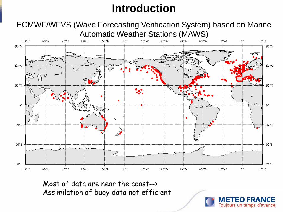
Introduction ECMWF/WFVS (Wave Forecasting Verification System) based on Marine
Automatic Weather Stations (MAWS)
Most of data are near the coast--> Assimilation of buoy data not efficient
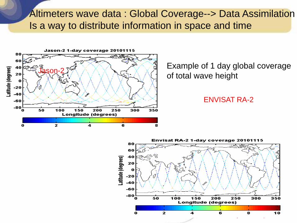
Jason-2
ENVISAT RA-2
Altimeters wave data : Global Coverage--> Data Assimilation Is a way to distribute information in space and time
Example of 1 day global coverage of total wave height
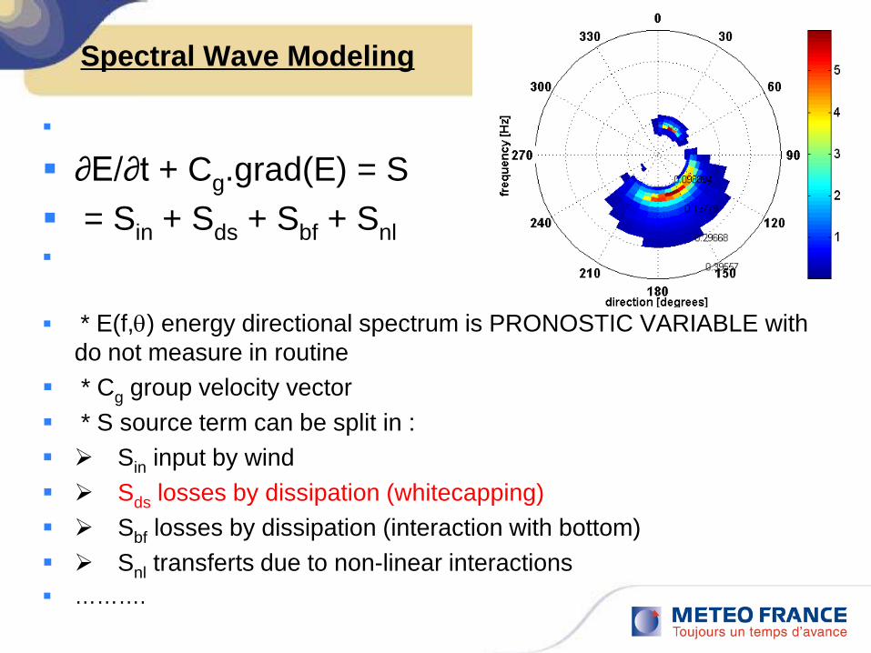
Spectral Wave Modeling
∂E/∂t + Cg.grad(E) = S = Sin + Sds + Sbf + Snl * E(f,θ) energy directional spectrum is PRONOSTIC VARIABLE with
do not measure in routine * Cg group velocity vector * S source term can be split in : Sin input by wind Sds losses by dissipation (whitecapping) Sbf losses by dissipation (interaction with bottom) Snl transferts due to non-linear interactions ……….
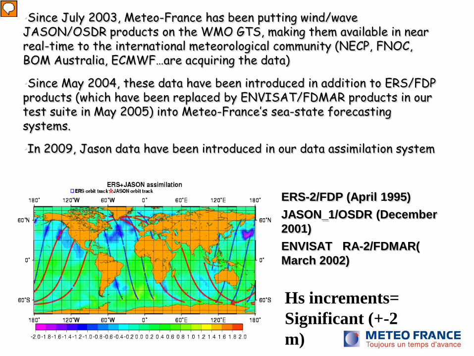
• ERS-2/FDP (April 1995) • JASON_1/OSDR (December
2001) • ENVISAT RA-2/FDMAR(
March 2002)
•Since July 2003, Meteo-France has been putting wind/wave JASON/OSDR products on the WMO GTS, making them available in near real-time to the international meteorological community (NECP, FNOC, BOM Australia, ECMWF…are acquiring the data)
•Since May 2004, these data have been introduced in addition to ERS/FDP products (which have been replaced by ENVISAT/FDMAR products in our test suite in May 2005) into Meteo-France’s sea-state forecasting systems.
•In 2009, Jason data have been introduced in our data assimilation system
Hs increments= Significant (+-2 m)
•Thomas J. 1988, QJRMS
•Janssen et al. 1989, JGR
•Lionnelo et al. 1992, JGR
•Lefèvre J.M., 1992, Proceeding of the 4th International Worshop on wave hincasting and Forecating QJRMS.
•Lemeur and Lefèvre 1995, Proceedings of Atelier de Modelisation de l'Atmosphère
•Greenslade 2001, JMS
•Skandrani and Lefèvre 2004, Marine Geodesy
•Greenslade and Young 2004, JGR : 2005 JAOS
Data Assimilation Techniques for wave forecasting : Background
Some work related to Spectral wave data (Buoys, SAR, RAR) OI -Voorips et al., 1997
-Aouf and al. Lefevre, 2006 JAOT, 2008 proceeding of ESAR/SEASAR
….. -Variational techniques : 2DVAR (x,y), 3DVAR (x,y,t) - De la Heras and Janssen 1992, JGR
- De Valk 1994, in Komen 1994
- Voorips and de valk 1997
Note : 3DVAR for waves similar to 4DVAR for atmosphere
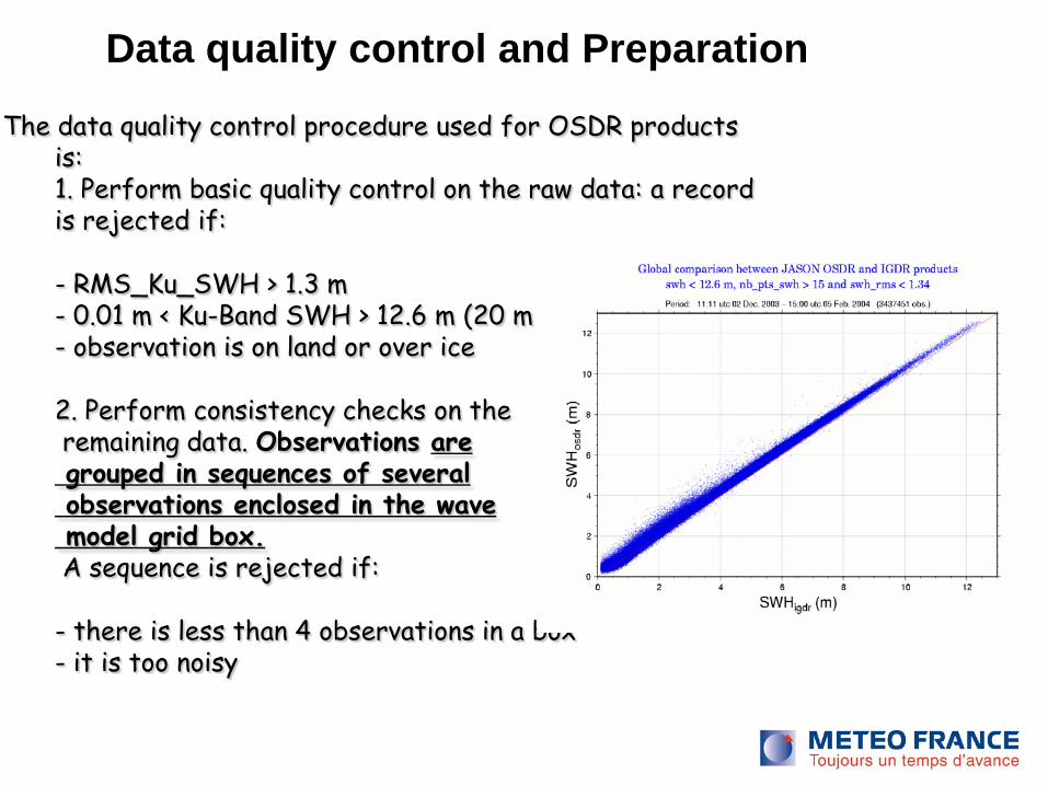
The data quality control procedure used for OSDR products is: 1. Perform basic quality control on the raw data: a record is rejected if:
- RMS_Ku_SWH > 1.3 m - 0.01 m < Ku-Band SWH > 12.6 m (20 m for others) - observation is on land or over ice
2. Perform consistency checks on the remaining data. Observations are grouped in sequences of several observations enclosed in the wave model grid box. A sequence is rejected if:
- there is less than 4 observations in a box - it is too noisy
Data quality control and Preparation
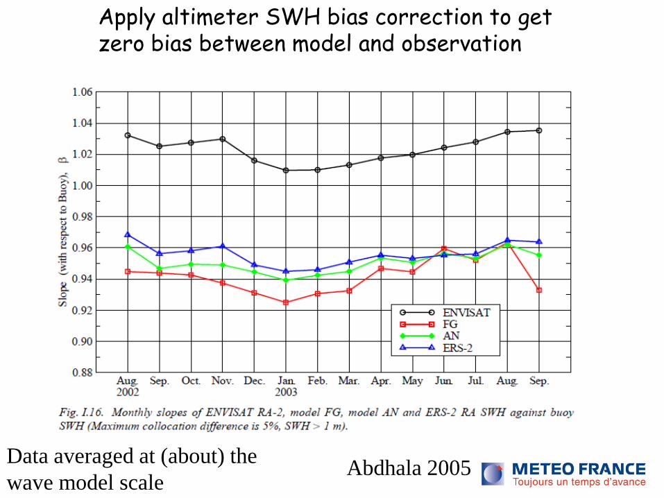
Abdhala 2005 Data averaged at (about) the wave model scale
Apply altimeter SWH bias correction to get zero bias between model and observation
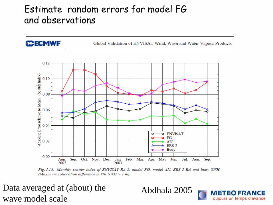
Abdhala 2005 Data averaged at (about) the wave model scale
Estimate random errors for model FG and observations
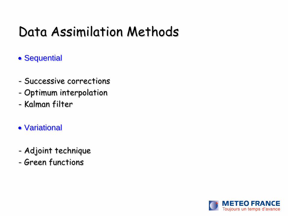
Data Assimilation Methods • Sequential - Successive corrections - Optimum interpolation - Kalman filter • Variational - Adjoint technique - Green functions
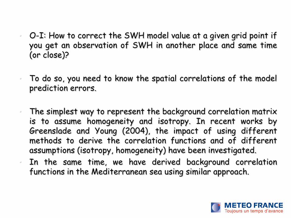
• O-I: How to correct the SWH model value at a given grid point if you get an observation of SWH in another place and same time (or close)?
• To do so, you need to know the spatial correlations of the model
prediction errors. • The simplest way to represent the background correlation matrix
is to assume homogeneity and isotropy. In recent works by Greenslade and Young (2004), the impact of using different methods to derive the correlation functions and of different assumptions (isotropy, homogeneity) have been investigated.
• In the same time, we have derived background correlation functions in the Mediterranean sea using similar approach.
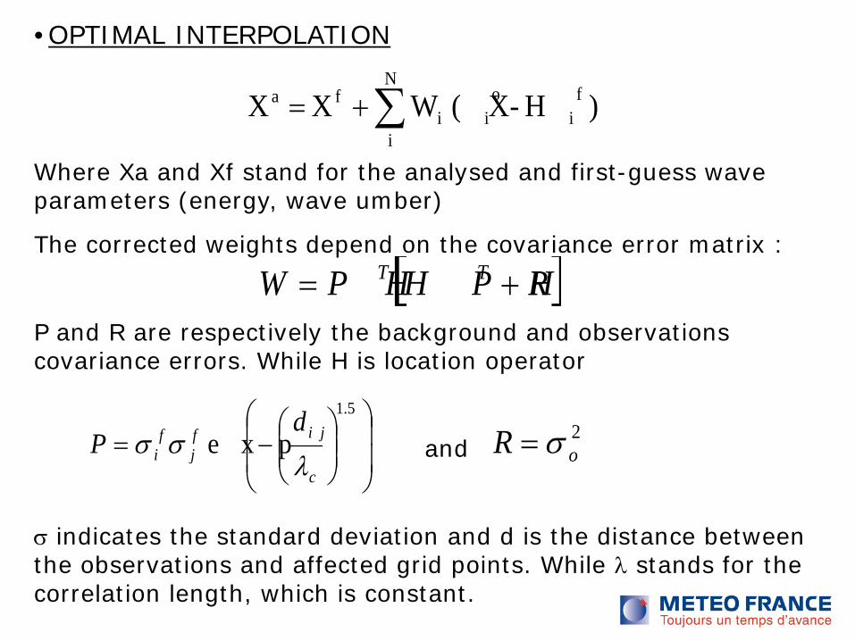
•OPTIMAL INTERPOLATION
Where Xa and Xf stand for the analysed and first-guess wave parameters (energy, wave umber)
The corrected weights depend on the covariance error matrix :
P and R are respectively the background and observations covariance errors. While H is location operator
and
σ indicates the standard deviation and d is the distance between the observations and affected grid points. While λ stands for the correlation length, which is constant.
∑+=N
i
fi
oii
fa )H-( X W X X
[ ]RH P HP HW TT +=
−=
5.1
e x pc
i jfj
fi
dP
λσσ 2
oR σ=
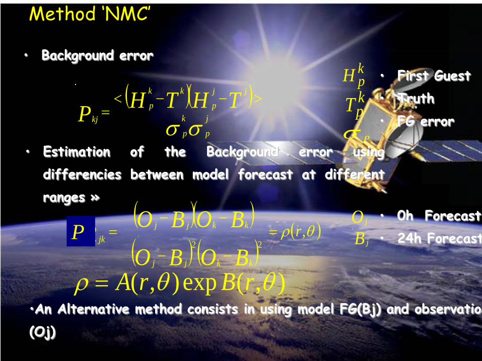
Method ‘NMC’
• Background error
( )( )σσ j
p
k
p
jjp
kkp
kjTHTHP
>−−<=
kpH
σ p
( )( )( ) ( )
( )θρ ,22
r
BOBOBOBOR
kkjj
kkjjjk =
−−
−−=
),(exp),( θθρ rBrA=
• First Guest • Truth • FG error
kpT
• Estimation of the Background error using differencies between model forecast at different ranges »
O j
B j
• 0h Forecast • 24h Forecast
•An Alternative method consists in using model FG(Bj) and observation (Oj)
P
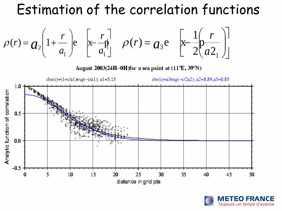
Estimation of the correlation functions
−=
13 22
1e x p)(arr aρ
−
+=
112 e x p1)(
ar
arr aρ
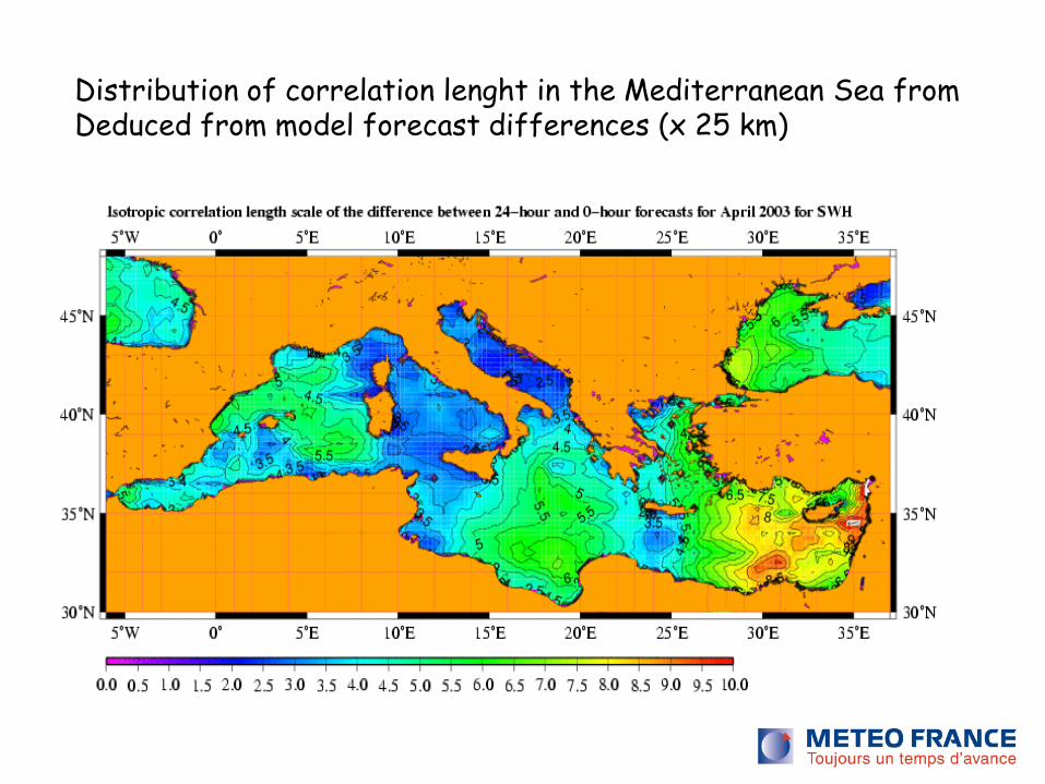
Distribution of correlation lenght in the Mediterranean Sea from Deduced from model forecast differences (x 25 km)
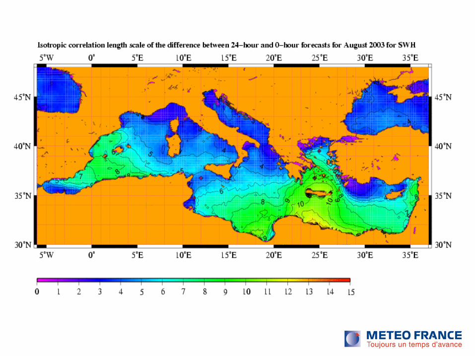

• Not homogenous as at global scale by Greenslade and Young (2004) but with smaller scales : average value around 100 km for the Medit and 300 km for Global with NMC
• Seasonally dependant : larger values in summer
In the Mediterranean Sea We have found the correlation functions to be:
Next Step – Update the Spectrum
Fa(f,θ)=A Fp(Bf,θ) B is very important, you have to shift the spectrum in the frequency space if the totel energy is changed (waves become longer as they growth !)
A and B coefficients are processed in different ways depending on wether wind sea is found in the guess spectrum or not.
If wind sea is dominant, dimensionless relations (Kidaigorodskii 62)
and a computed dimensionless growth curve (depending on the wave model used) are used to estimate A and B
If Swell is dominant, A and B are processed in such a way that the
average steepness is conserved : s=Ekm2/4pi2
This method relies on 3 main assumptions -the ratio windSea/Swell is correct -the duration of the wind sea is correct -the wind direction is correct
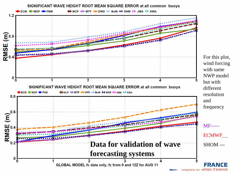
For this plot, wind forcing with same NWP model but with different resolution and frequency
MF-----
ECMWF__
SHOM --- Data for validation of wave forecasting systems
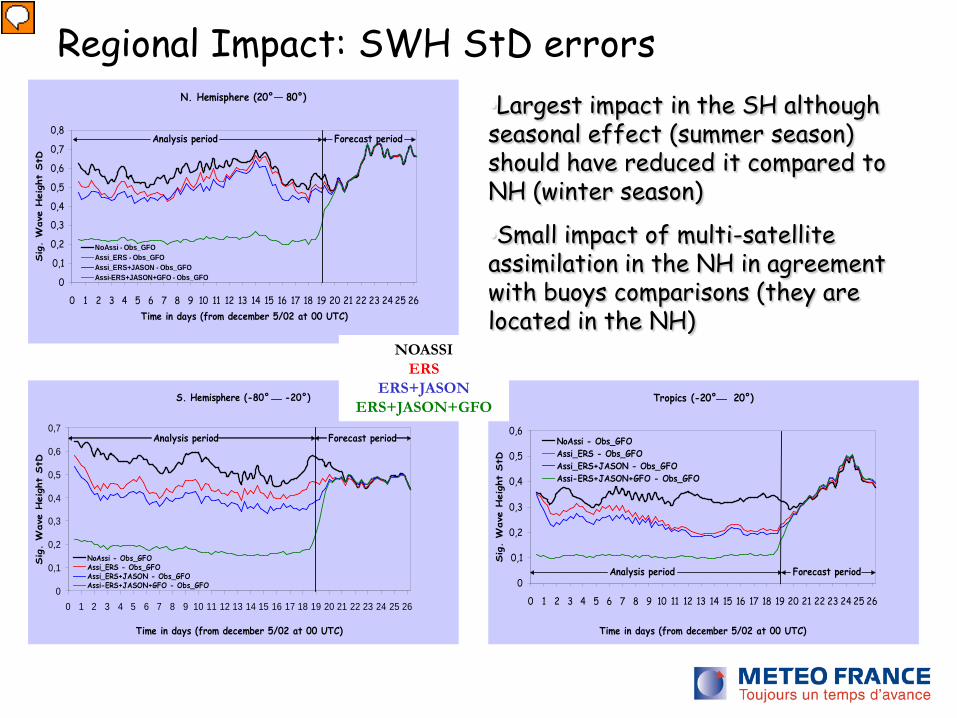
Regional Impact: SWH StD errors N. Hemisphere (20° 80°)
0
0,1
0,2
0,3
0,4
0,5
0,6
0,7
0,8
0 1 2 3 4 5 6 7 8 9 10 11 12 13 14 15 16 17 18 19 20 21 22 23 24 25 26Time in days (from december 5/02 at 00 UTC)
Sig. W
ave
Heigh
t StD
NoAssi - Obs_GFOAssi_ERS - Obs_GFOAssi_ERS+JASON - Obs_GFOAssi-ERS+JASON+GFO - Obs_GFO
Analysis period Forecast period
Tropics (-20° 20°)
0
0,1
0,2
0,3
0,4
0,5
0,6
0 1 2 3 4 5 6 7 8 9 10 11 12 13 14 15 16 17 18 19 20 21 22 23 24 25 26
Time in days (from december 5/02 at 00 UTC)
Sig. W
ave
Heigh
t StD
NoAssi - Obs_GFOAssi_ERS - Obs_GFOAssi_ERS+JASON - Obs_GFOAssi-ERS+JASON+GFO - Obs_GFO
Analysis period Forecast period
S. Hemisphere (-80° -20°)
0
0,1
0,2
0,3
0,4
0,5
0,6
0,7
0 1 2 3 4 5 6 7 8 9 10 11 12 13 14 15 16 17 18 19 20 21 22 23 24 25 26
Time in days (from december 5/02 at 00 UTC)
Sig. W
ave
Heigh
t StD
NoAssi - Obs_GFOAssi_ERS - Obs_GFOAssi_ERS+JASON - Obs_GFOAssi-ERS+JASON+GFO - Obs_GFO
Analysis period Forecast period
•Largest impact in the SH although seasonal effect (summer season) should have reduced it compared to NH (winter season)
•Small impact of multi-satellite assimilation in the NH in agreement with buoys comparisons (they are located in the NH)
NOASSI ERS
ERS+JASON ERS+JASON+GFO
NWS assimilating RA data - ECMWF - Meteo-France - FNMOC NWS implementing RA data assimilation - NOAA NWS having assimilate RA data in the past -MetOffice -BOM -KNMI
Operational Wave Data Assimilation
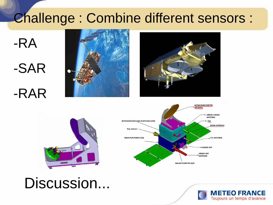
Challenge : Combine different sensors :
-RA
-SAR
-RAR
Discussion...