The AMath and DAMath

Special Functions

Reference Manual

and

Implementation Notes

Version 2.19

Including Complex Functions

Wolfgang Ehrhardt

March 2018

Copyright c© 2009-2018 Wolfgang Ehrhardt

This electronic manual (”work”) is distributed under the terms and conditions of the”Creative Commons license Attribution - Noncommercial - No Derivative Works 3.0”1.This is not a license, but a human-readable summary of the full license from:

http://creativecommons.org/licenses/by-nc-nd/3.0/

You are free to copy, distribute and transmit this manual under the following conditions:

• Attribution. You must attribute the work in the manner specified by the author orlicensor (but not in any way that suggests that they endorse you or your use of thework)

• Noncommercial. You may not use this work for commercial purposes.

• No Derivative Works. You may not alter, transform, or build upon this work.

With the understanding that:

• Any of the above conditions can be waived if you get permission from the copyrightholder.

• Where the work or any of its elements is in the public domain under applicable law,that status is in no way affected by the license.

• In no way are any of the following rights affected by the license:

– Your fair dealing or fair use rights, or other applicable copyright exceptions andlimitations;

– The author’s moral rights;

– Rights other persons may have either in the work itself or in how the work isused, such as publicity or privacy rights.

For any reuse or distribution, you must make clear to others the license terms of this work.The best way to do this is with a link to the URL given above.

1 The license type may change in future versions of this text.

2

Contents

1 Introduction 13

2 AMath and DAMath 142.1 AMath functions . . . . . . . . . . . . . . . . . . . . . . . . . . . . . . . . 142.2 DAMath functions and special functions . . . . . . . . . . . . . . . . . . . 15

2.2.1 DAMath functions . . . . . . . . . . . . . . . . . . . . . . . . . . . 152.2.2 DAMath special functions . . . . . . . . . . . . . . . . . . . . . . . 15

3 Special functions 163.1 Bessel functions and related . . . . . . . . . . . . . . . . . . . . . . . . . . 17

3.1.1 Bessel functions of integer order . . . . . . . . . . . . . . . . . . . 173.1.1.1 J0(x) . . . . . . . . . . . . . . . . . . . . . . . . . . . . . 173.1.1.2 J1(x) . . . . . . . . . . . . . . . . . . . . . . . . . . . . . 173.1.1.3 Jn(x) . . . . . . . . . . . . . . . . . . . . . . . . . . . . . 173.1.1.4 Y0(x) . . . . . . . . . . . . . . . . . . . . . . . . . . . . . 183.1.1.5 Y1(x) . . . . . . . . . . . . . . . . . . . . . . . . . . . . . 183.1.1.6 Yn(x) . . . . . . . . . . . . . . . . . . . . . . . . . . . . . 18

3.1.2 Modified Bessel functions of integer order . . . . . . . . . . . . . . 193.1.2.1 I0(x) . . . . . . . . . . . . . . . . . . . . . . . . . . . . . 193.1.2.2 Exponentially scaled I0,e(x) . . . . . . . . . . . . . . . . 193.1.2.3 I1(x) . . . . . . . . . . . . . . . . . . . . . . . . . . . . . 193.1.2.4 Exponentially scaled I1,e(x) . . . . . . . . . . . . . . . . 193.1.2.5 In(x) . . . . . . . . . . . . . . . . . . . . . . . . . . . . . 203.1.2.6 K0(x) . . . . . . . . . . . . . . . . . . . . . . . . . . . . . 203.1.2.7 Exponentially scaled K0,e(x) . . . . . . . . . . . . . . . . 203.1.2.8 K1(x) . . . . . . . . . . . . . . . . . . . . . . . . . . . . . 203.1.2.9 Exponentially scaled K1,e(x) . . . . . . . . . . . . . . . . 203.1.2.10 Kn(x) . . . . . . . . . . . . . . . . . . . . . . . . . . . . . 21

3.1.3 Bessel functions of real order . . . . . . . . . . . . . . . . . . . . . 213.1.3.1 Jν(x) . . . . . . . . . . . . . . . . . . . . . . . . . . . . . 223.1.3.2 Yν(x) . . . . . . . . . . . . . . . . . . . . . . . . . . . . . 223.1.3.3 Bessel Λν(x) . . . . . . . . . . . . . . . . . . . . . . . . . 23

3.1.4 Modified Bessel functions of real order . . . . . . . . . . . . . . . . 233.1.4.1 Iν(x) . . . . . . . . . . . . . . . . . . . . . . . . . . . . . 233.1.4.2 Exponentially scaled Iν,e(x) . . . . . . . . . . . . . . . . 243.1.4.3 Kν(x) . . . . . . . . . . . . . . . . . . . . . . . . . . . . . 243.1.4.4 Exponentially scaled Kν,e(x) . . . . . . . . . . . . . . . . 24

3.1.5 Airy functions . . . . . . . . . . . . . . . . . . . . . . . . . . . . . 24

3

3.1.5.1 Airy Ai(x) . . . . . . . . . . . . . . . . . . . . . . . . . . 253.1.5.2 Airy Bi(x) . . . . . . . . . . . . . . . . . . . . . . . . . . 253.1.5.3 Airy Ai’(x) . . . . . . . . . . . . . . . . . . . . . . . . . . 263.1.5.4 Airy Bi’(x) . . . . . . . . . . . . . . . . . . . . . . . . . . 263.1.5.5 Scaled Airy Ais(x) . . . . . . . . . . . . . . . . . . . . . . 263.1.5.6 Scaled Airy Bis(x) . . . . . . . . . . . . . . . . . . . . . . 263.1.5.7 Airy Gi(x) . . . . . . . . . . . . . . . . . . . . . . . . . . 273.1.5.8 Airy Hi(x) . . . . . . . . . . . . . . . . . . . . . . . . . . 27

3.1.6 Kelvin functions . . . . . . . . . . . . . . . . . . . . . . . . . . . . 273.1.6.1 Kelvin functions ber(x) and bei(x) . . . . . . . . . . . . . 293.1.6.2 Kelvin functions ker(x) and kei(x) . . . . . . . . . . . . . 293.1.6.3 Kelvin function ber(x) . . . . . . . . . . . . . . . . . . . . 293.1.6.4 Kelvin function bei(x) . . . . . . . . . . . . . . . . . . . . 293.1.6.5 Kelvin function ker(x) . . . . . . . . . . . . . . . . . . . . 293.1.6.6 Kelvin function kei(x) . . . . . . . . . . . . . . . . . . . . 29

3.1.7 Spherical Bessel functions . . . . . . . . . . . . . . . . . . . . . . . 303.1.7.1 Spherical Bessel function jn(x) . . . . . . . . . . . . . . . 303.1.7.2 Spherical Bessel function yn(x) . . . . . . . . . . . . . . 303.1.7.3 Modified spherical Bessel function in(x) . . . . . . . . . . 303.1.7.4 Exponentially scaled in,e(x) . . . . . . . . . . . . . . . . 303.1.7.5 Modified spherical Bessel function kn(x) . . . . . . . . . 313.1.7.6 Exponentially scaled kn,e(x) . . . . . . . . . . . . . . . . 31

3.1.8 Struve functions . . . . . . . . . . . . . . . . . . . . . . . . . . . . 313.1.8.1 Struve H0(x) . . . . . . . . . . . . . . . . . . . . . . . . . 323.1.8.2 Struve H1(x) . . . . . . . . . . . . . . . . . . . . . . . . . 323.1.8.3 Struve function Hν(x) . . . . . . . . . . . . . . . . . . . . 323.1.8.4 Modified Struve function Lν(x) . . . . . . . . . . . . . . 323.1.8.5 Struve L0(x) . . . . . . . . . . . . . . . . . . . . . . . . . 333.1.8.6 Struve L1(x) . . . . . . . . . . . . . . . . . . . . . . . . . 33

3.2 Elliptic integrals, elliptic and theta functions . . . . . . . . . . . . . . . . 343.2.1 Legendre style elliptic integrals . . . . . . . . . . . . . . . . . . . . 34

3.2.1.1 Complete elliptic integral of the 1st kind . . . . . . . . . 343.2.1.2 Complete elliptic integral of the 2nd kind . . . . . . . . . 343.2.1.3 Complete elliptic integral of the 3rd kind . . . . . . . . . 343.2.1.4 Complete elliptic integral B(k) . . . . . . . . . . . . . . . 353.2.1.5 Complete elliptic integral D(k) . . . . . . . . . . . . . . . 353.2.1.6 Legendre elliptic integral of the 1st kind . . . . . . . . . . 353.2.1.7 Legendre elliptic integral of the 2nd kind . . . . . . . . . 363.2.1.8 Legendre elliptic integral of the 3rd kind . . . . . . . . . 363.2.1.9 Legendre elliptic integral B(ϕ,k) . . . . . . . . . . . . . . 373.2.1.10 Legendre elliptic integral D(ϕ,k) . . . . . . . . . . . . . 37

3.2.2 Carlson style elliptic integrals . . . . . . . . . . . . . . . . . . . . . 383.2.2.1 Degenerate elliptic integral RC . . . . . . . . . . . . . . . 383.2.2.2 Integral of the 1st kind RF . . . . . . . . . . . . . . . . . 383.2.2.3 Integral of the 2nd kind RD . . . . . . . . . . . . . . . . 383.2.2.4 Integral of the 2nd kind RG . . . . . . . . . . . . . . . . 393.2.2.5 Integral of the 3rd kind RJ . . . . . . . . . . . . . . . . . 39

3.2.3 Bulirsch style elliptic integrals . . . . . . . . . . . . . . . . . . . . 393.2.3.1 Complete integral of the 1st kind cel1 . . . . . . . . . . . 393.2.3.2 Complete integral of the 2nd kind cel2 . . . . . . . . . . . 40

4

3.2.3.3 General complete integral cel . . . . . . . . . . . . . . . . 403.2.3.4 Incomplete integral of the 1st kind el1 . . . . . . . . . . . 403.2.3.5 Incomplete integral of the 2nd kind el2 . . . . . . . . . . 403.2.3.6 Incomplete integral of the 3rd kind el3 . . . . . . . . . . . 41

3.2.4 Maple style elliptic integrals . . . . . . . . . . . . . . . . . . . . . . 413.2.4.1 Complete integral of the 1st kind EllipticK . . . . . . . . 413.2.4.2 Complete integral of the 1st kind for imaginary modulus 413.2.4.3 Complementary complete integral of the 1st kind . . . . . 423.2.4.4 Complete integral of the 2nd kind EllipticEC . . . . . . . 423.2.4.5 Complete integral of the 2nd kind for imaginary modulus 423.2.4.6 Complementary complete integral of the 2nd kind . . . . 433.2.4.7 Complete integral of the 3rd kind EllipticPiC . . . . . . . 433.2.4.8 Complementary complete integral of the 3rd kind . . . . 433.2.4.9 Incomplete integral of the 1st kind EllipticF . . . . . . . 433.2.4.10 Incomplete integral of the 2nd kind EllipticE . . . . . . . 443.2.4.11 Incomplete integral of the 3rd kind EllipticPi . . . . . . . 44

3.2.5 Heuman’s Lambda function . . . . . . . . . . . . . . . . . . . . . . 443.2.6 Jacobi Zeta function . . . . . . . . . . . . . . . . . . . . . . . . . . 453.2.7 Elliptic modulus . . . . . . . . . . . . . . . . . . . . . . . . . . . . 453.2.8 Elliptic nome . . . . . . . . . . . . . . . . . . . . . . . . . . . . . . 453.2.9 Jacobi amplitude . . . . . . . . . . . . . . . . . . . . . . . . . . . . 463.2.10 Jacobi elliptic functions . . . . . . . . . . . . . . . . . . . . . . . . 46

3.2.10.1 Jacobi elliptic function sn . . . . . . . . . . . . . . . . . . 463.2.10.2 Jacobi elliptic function cn . . . . . . . . . . . . . . . . . . 473.2.10.3 Jacobi elliptic function dn . . . . . . . . . . . . . . . . . . 473.2.10.4 Jacobi elliptic function nc . . . . . . . . . . . . . . . . . . 473.2.10.5 Jacobi elliptic function sc . . . . . . . . . . . . . . . . . . 473.2.10.6 Jacobi elliptic function dc . . . . . . . . . . . . . . . . . . 473.2.10.7 Jacobi elliptic function nd . . . . . . . . . . . . . . . . . . 473.2.10.8 Jacobi elliptic function sd . . . . . . . . . . . . . . . . . . 473.2.10.9 Jacobi elliptic function cd . . . . . . . . . . . . . . . . . . 483.2.10.10 Jacobi elliptic function ns . . . . . . . . . . . . . . . . . . 483.2.10.11 Jacobi elliptic function cs . . . . . . . . . . . . . . . . . . 483.2.10.12 Jacobi elliptic function ds . . . . . . . . . . . . . . . . . . 48

3.2.11 Inverse Jacobi elliptic functions . . . . . . . . . . . . . . . . . . . . 483.2.11.1 Inverse Jacobi elliptic function arcsn . . . . . . . . . . . . 493.2.11.2 Inverse Jacobi elliptic function arccn . . . . . . . . . . . . 493.2.11.3 Inverse Jacobi elliptic function arcdn . . . . . . . . . . . 493.2.11.4 Inverse Jacobi elliptic function arccd . . . . . . . . . . . . 503.2.11.5 Inverse Jacobi elliptic function arcsd . . . . . . . . . . . . 503.2.11.6 Inverse Jacobi elliptic function arcnd . . . . . . . . . . . 503.2.11.7 Inverse Jacobi elliptic function arcdc . . . . . . . . . . . . 513.2.11.8 Inverse Jacobi elliptic function arcnc . . . . . . . . . . . . 513.2.11.9 Inverse Jacobi elliptic function arcsc . . . . . . . . . . . . 513.2.11.10 Inverse Jacobi elliptic function arcns . . . . . . . . . . . . 513.2.11.11 Inverse Jacobi elliptic function arcds . . . . . . . . . . . . 523.2.11.12 Inverse Jacobi elliptic function arccs . . . . . . . . . . . . 52

3.2.12 Jacobi theta functions . . . . . . . . . . . . . . . . . . . . . . . . . 523.2.13 Jacobi theta functions at zero . . . . . . . . . . . . . . . . . . . . . 53

3.2.13.1 Jacobi theta1p(q) . . . . . . . . . . . . . . . . . . . . . . 54

5

3.2.13.2 Jacobi theta2(q) . . . . . . . . . . . . . . . . . . . . . . . 543.2.13.3 Jacobi theta3(q) . . . . . . . . . . . . . . . . . . . . . . . 543.2.13.4 Jacobi theta4(q) . . . . . . . . . . . . . . . . . . . . . . . 54

3.2.14 Lemniscate functions . . . . . . . . . . . . . . . . . . . . . . . . . . 553.2.14.1 sin lemn (x) . . . . . . . . . . . . . . . . . . . . . . . . . 553.2.14.2 cos lemn (x) . . . . . . . . . . . . . . . . . . . . . . . . . 55

3.3 Error function and related . . . . . . . . . . . . . . . . . . . . . . . . . . . 563.3.1 Dawson’s integral . . . . . . . . . . . . . . . . . . . . . . . . . . . . 563.3.2 Generalized Dawson integral . . . . . . . . . . . . . . . . . . . . . 563.3.3 Error function erf . . . . . . . . . . . . . . . . . . . . . . . . . . . . 563.3.4 Generalized error function erfg . . . . . . . . . . . . . . . . . . . . 573.3.5 Complementary error function erfc . . . . . . . . . . . . . . . . . . 573.3.6 Exponentially scaled complementary error function . . . . . . . . . 573.3.7 Scaled repeated integrals of erfc . . . . . . . . . . . . . . . . . . . . 583.3.8 Imaginary error function erfi . . . . . . . . . . . . . . . . . . . . . 583.3.9 Difference of error functions erfh(x,h) . . . . . . . . . . . . . . . . 593.3.10 Difference of error functions erf2(x1,x2) . . . . . . . . . . . . . . . 593.3.11 Inverse error functions . . . . . . . . . . . . . . . . . . . . . . . . . 59

3.3.11.1 Inverse of erf . . . . . . . . . . . . . . . . . . . . . . . . . 593.3.11.2 Inverse of erfc . . . . . . . . . . . . . . . . . . . . . . . . 593.3.11.3 Inverse of erfce . . . . . . . . . . . . . . . . . . . . . . . . 603.3.11.4 Inverse of erfi . . . . . . . . . . . . . . . . . . . . . . . . . 60

3.3.12 Probability functions . . . . . . . . . . . . . . . . . . . . . . . . . . 603.3.12.1 P(x) . . . . . . . . . . . . . . . . . . . . . . . . . . . . . . 603.3.12.2 Q(x) . . . . . . . . . . . . . . . . . . . . . . . . . . . . . . 603.3.12.3 Z(x) . . . . . . . . . . . . . . . . . . . . . . . . . . . . . . 61

3.3.13 Expint3 . . . . . . . . . . . . . . . . . . . . . . . . . . . . . . . . . 613.3.14 Fresnel integrals . . . . . . . . . . . . . . . . . . . . . . . . . . . . 613.3.15 Fresnel auxiliary functions . . . . . . . . . . . . . . . . . . . . . . . 623.3.16 Goodwin-Staton integral . . . . . . . . . . . . . . . . . . . . . . . . 623.3.17 Marcum Q functions . . . . . . . . . . . . . . . . . . . . . . . . . . 623.3.18 Owen’s T function . . . . . . . . . . . . . . . . . . . . . . . . . . . 63

3.4 Exponential integrals and related . . . . . . . . . . . . . . . . . . . . . . . 643.4.1 Hyperbolic cosine integral Chi . . . . . . . . . . . . . . . . . . . . 643.4.2 Cosine integral Ci . . . . . . . . . . . . . . . . . . . . . . . . . . . 643.4.3 Entire cosine integral Cin . . . . . . . . . . . . . . . . . . . . . . . 643.4.4 Entire hyperbolic cosine integral Cinh . . . . . . . . . . . . . . . . 653.4.5 Exponential integral E1 . . . . . . . . . . . . . . . . . . . . . . . . 653.4.6 Scaled exponential integral E1 . . . . . . . . . . . . . . . . . . . . 653.4.7 Exponential integral Ei . . . . . . . . . . . . . . . . . . . . . . . . 653.4.8 Scaled exponential integral Ei(x) . . . . . . . . . . . . . . . . . . . 663.4.9 Scaled exponential integral Ei(x2) . . . . . . . . . . . . . . . . . . 663.4.10 Inverse of the exponential integral Ei . . . . . . . . . . . . . . . . . 663.4.11 Entire exponential integral Ein . . . . . . . . . . . . . . . . . . . . 663.4.12 Exponential integrals En . . . . . . . . . . . . . . . . . . . . . . . . 673.4.13 Generalized exponential integrals Ep . . . . . . . . . . . . . . . . . 673.4.14 Logarithmic integral li . . . . . . . . . . . . . . . . . . . . . . . . . 683.4.15 Inverse of the logarithmic integral . . . . . . . . . . . . . . . . . . 683.4.16 Hyperbolic sine integral Shi . . . . . . . . . . . . . . . . . . . . . . 693.4.17 Sine integral Si . . . . . . . . . . . . . . . . . . . . . . . . . . . . . 69

6

3.4.18 Shifted sine integral si . . . . . . . . . . . . . . . . . . . . . . . . . 693.5 Gamma function and related . . . . . . . . . . . . . . . . . . . . . . . . . 70

3.5.1 Gamma functions . . . . . . . . . . . . . . . . . . . . . . . . . . . . 703.5.1.1 Gamma function Γ(x) . . . . . . . . . . . . . . . . . . . . 703.5.1.2 Gamma function Γ(1 + x)− 1 . . . . . . . . . . . . . . . 713.5.1.3 Inverse of Γ . . . . . . . . . . . . . . . . . . . . . . . . . . 713.5.1.4 Temme’s regulated gamma function Γ∗(x) . . . . . . . . 713.5.1.5 Logarithm of the gamma function . . . . . . . . . . . . . 713.5.1.6 Inverse of lnΓ . . . . . . . . . . . . . . . . . . . . . . . . 723.5.1.7 Logarithm of Γ(1 + x) . . . . . . . . . . . . . . . . . . . 723.5.1.8 Reciprocal gamma function . . . . . . . . . . . . . . . . . 723.5.1.9 Sign of gamma function . . . . . . . . . . . . . . . . . . . 723.5.1.10 Logarithm and sign of gamma function . . . . . . . . . . 72

3.5.2 Incomplete gamma functions . . . . . . . . . . . . . . . . . . . . . 733.5.2.1 Normalised incomplete gamma functions . . . . . . . . . 733.5.2.2 Non-normalised incomplete gamma functions . . . . . . . 743.5.2.3 Tricomi’s entire incomplete gamma function . . . . . . . 743.5.2.4 Inverse normalised incomplete gamma functions . . . . . 75

3.5.3 Beta functions . . . . . . . . . . . . . . . . . . . . . . . . . . . . . 763.5.3.1 Beta function B(x,y) . . . . . . . . . . . . . . . . . . . . . 763.5.3.2 Logarithm of the beta function . . . . . . . . . . . . . . . 763.5.3.3 Normalised incomplete beta function . . . . . . . . . . . 773.5.3.4 Non-normalised incomplete beta function . . . . . . . . . 773.5.3.5 Inverse normalised incomplete beta function . . . . . . . 78

3.5.4 Factorials, Pochhammer symbol, binomial coefficient . . . . . . . . 783.5.4.1 Factorial . . . . . . . . . . . . . . . . . . . . . . . . . . . 783.5.4.2 Double factorial . . . . . . . . . . . . . . . . . . . . . . . 783.5.4.3 Logarithm of factorials . . . . . . . . . . . . . . . . . . . 783.5.4.4 Binomial coefficient . . . . . . . . . . . . . . . . . . . . . 793.5.4.5 Pochhammer symbol . . . . . . . . . . . . . . . . . . . . 793.5.4.6 Relative Pochhammer symbol . . . . . . . . . . . . . . . 80

3.5.5 Ratio of gamma functions . . . . . . . . . . . . . . . . . . . . . . . 803.5.6 Psi and polygamma functions . . . . . . . . . . . . . . . . . . . . . 80

3.5.6.1 Digamma function ψ(x) . . . . . . . . . . . . . . . . . . . 803.5.6.2 Trigamma function ψ′(x) . . . . . . . . . . . . . . . . . . 813.5.6.3 Tetragamma function ψ′′(x) . . . . . . . . . . . . . . . . 813.5.6.4 Pentagamma function ψ′′′(x) . . . . . . . . . . . . . . . . 813.5.6.5 Polygamma function ψ(n)(x) . . . . . . . . . . . . . . . . 813.5.6.6 Inverse digamma function ψ−1(y) . . . . . . . . . . . . . 823.5.6.7 Bateman function G(x) . . . . . . . . . . . . . . . . . . . 83

3.6 Zeta functions, polylogarithms, and related . . . . . . . . . . . . . . . . . 843.6.1 Riemann zeta functions . . . . . . . . . . . . . . . . . . . . . . . . 84

3.6.1.1 Riemann ζ(s) function . . . . . . . . . . . . . . . . . . . 843.6.1.2 Riemann ζ(n) for integer arguments . . . . . . . . . . . . 843.6.1.3 Riemann ζ(1 + x) . . . . . . . . . . . . . . . . . . . . . . 853.6.1.4 Riemann ζ(s)− 1 . . . . . . . . . . . . . . . . . . . . . . 85

3.6.2 Prime zeta function . . . . . . . . . . . . . . . . . . . . . . . . . . 853.6.3 Dirichlet eta functions . . . . . . . . . . . . . . . . . . . . . . . . . 86

3.6.3.1 Dirichlet eta function . . . . . . . . . . . . . . . . . . . . 86

7

3.6.3.2 Dirichlet eta function for integer arguments . . . . . . . . 863.6.3.3 Dirichlet η(s)− 1 . . . . . . . . . . . . . . . . . . . . . . 86

3.6.4 Dirichlet beta function . . . . . . . . . . . . . . . . . . . . . . . . . 863.6.5 Dirichlet lambda function . . . . . . . . . . . . . . . . . . . . . . . 873.6.6 Hurwitz zeta function . . . . . . . . . . . . . . . . . . . . . . . . . 873.6.7 Bose-Einstein integrals of real order . . . . . . . . . . . . . . . . . 883.6.8 Fermi-Dirac integrals . . . . . . . . . . . . . . . . . . . . . . . . . . 88

3.6.8.1 Fermi-Dirac integrals of real order . . . . . . . . . . . . . 883.6.8.2 Fermi-Dirac integrals of integer order . . . . . . . . . . . 893.6.8.3 Fermi-Dirac integral F−1/2(x) . . . . . . . . . . . . . . . 893.6.8.4 Fermi-Dirac integral F1/2(x) . . . . . . . . . . . . . . . . 893.6.8.5 Fermi-Dirac integral F3/2(x) . . . . . . . . . . . . . . . . 893.6.8.6 Fermi-Dirac integral F5/2(x) . . . . . . . . . . . . . . . . 89

3.6.9 Legendre’s Chi-function . . . . . . . . . . . . . . . . . . . . . . . . 903.6.10 Lerch’s transcendent . . . . . . . . . . . . . . . . . . . . . . . . . . 903.6.11 Polylogarithms of integer order . . . . . . . . . . . . . . . . . . . . 913.6.12 Polylogarithms of real order . . . . . . . . . . . . . . . . . . . . . . 923.6.13 Dilogarithm function . . . . . . . . . . . . . . . . . . . . . . . . . . 933.6.14 Trilogarithm function . . . . . . . . . . . . . . . . . . . . . . . . . 933.6.15 Clausen function Cl2(x) . . . . . . . . . . . . . . . . . . . . . . . . 943.6.16 Inverse-tangent integral Ti2(x) . . . . . . . . . . . . . . . . . . . . 943.6.17 Inverse-tangent integral of real order . . . . . . . . . . . . . . . . . 953.6.18 Lobachevsky’s log-cos integral . . . . . . . . . . . . . . . . . . . . . 953.6.19 Lobachevsky’s log-sin integral . . . . . . . . . . . . . . . . . . . . . 953.6.20 Harmonic number function Hx . . . . . . . . . . . . . . . . . . . . 963.6.21 Generalized harmonic number function H(r)

x . . . . . . . . . . . . . 963.7 Orthogonal polynomials and Legendre functions . . . . . . . . . . . . . . . 97

3.7.1 Chebyshev polynomials of the first kind . . . . . . . . . . . . . . . 973.7.2 Chebyshev polynomials of the second kind . . . . . . . . . . . . . . 973.7.3 Chebyshev polynomials of the third kind . . . . . . . . . . . . . . . 983.7.4 Chebyshev polynomials of the fourth kind . . . . . . . . . . . . . . 983.7.5 Chebyshev function of the first kind . . . . . . . . . . . . . . . . . 993.7.6 Gegenbauer (ultraspherical) polynomials . . . . . . . . . . . . . . . 993.7.7 Hermite polynomials Hn . . . . . . . . . . . . . . . . . . . . . . . . 993.7.8 Hermite polynomials Hen . . . . . . . . . . . . . . . . . . . . . . . 1003.7.9 Jacobi polynomials . . . . . . . . . . . . . . . . . . . . . . . . . . . 1003.7.10 Generalized Laguerre polynomials . . . . . . . . . . . . . . . . . . 1003.7.11 Laguerre polynomials . . . . . . . . . . . . . . . . . . . . . . . . . 1013.7.12 Associated Laguerre polynomials . . . . . . . . . . . . . . . . . . . 1013.7.13 Legendre polynomials / functions . . . . . . . . . . . . . . . . . . . 1013.7.14 Associated Legendre polynomials / functions . . . . . . . . . . . . 1023.7.15 Legendre functions of the second kind . . . . . . . . . . . . . . . . 1023.7.16 Associated Legendre functions of the second kind . . . . . . . . . . 1033.7.17 Spherical harmonic functions . . . . . . . . . . . . . . . . . . . . . 1033.7.18 Some toroidal harmonic functions . . . . . . . . . . . . . . . . . . . 1043.7.19 Zernike radial polynomials . . . . . . . . . . . . . . . . . . . . . . . 105

3.8 Hypergeometric functions and related . . . . . . . . . . . . . . . . . . . . 1063.8.1 Gauss hypergeometric function F(a,b;c;x) . . . . . . . . . . . . . . 1063.8.2 Regularized Gauss hypergeometric function . . . . . . . . . . . . . 1073.8.3 Kummer’s confluent hypergeometric function M(a,b,x) . . . . . . . 107

8

3.8.4 Regularized Kummer function . . . . . . . . . . . . . . . . . . . . . 1083.8.5 Tricomi’s confluent hypergeometric function U(a,b,x) . . . . . . . . 1083.8.6 Confluent hypergeometric limit function 0F1(b,x) . . . . . . . . . 1093.8.7 Regularized confluent hypergeometric limit function . . . . . . . . 1103.8.8 Whittaker M function . . . . . . . . . . . . . . . . . . . . . . . . . 1103.8.9 Whittaker W function . . . . . . . . . . . . . . . . . . . . . . . . . 1113.8.10 Parabolic cylinder functions . . . . . . . . . . . . . . . . . . . . . . 111

3.8.10.1 Parabolic cylinder function Dν(x) . . . . . . . . . . . . . 1113.8.10.2 Parabolic cylinder function U(a,x) . . . . . . . . . . . . 1113.8.10.3 Parabolic cylinder function V(a,x) . . . . . . . . . . . . 1123.8.10.4 Hermite function Hν(x) . . . . . . . . . . . . . . . . . . . 113

3.9 Statistical distributions . . . . . . . . . . . . . . . . . . . . . . . . . . . . 1143.9.1 Erlang, geometric, and Pascal distributions . . . . . . . . . . . . . 1143.9.2 Beta distribution . . . . . . . . . . . . . . . . . . . . . . . . . . . . 1143.9.3 Binomial distribution . . . . . . . . . . . . . . . . . . . . . . . . . 1153.9.4 Cauchy distribution . . . . . . . . . . . . . . . . . . . . . . . . . . 1153.9.5 Chi distribution . . . . . . . . . . . . . . . . . . . . . . . . . . . . 1153.9.6 Chi-square distribution . . . . . . . . . . . . . . . . . . . . . . . . 1163.9.7 Exponential distribution . . . . . . . . . . . . . . . . . . . . . . . . 1163.9.8 Extreme Value Type I distribution . . . . . . . . . . . . . . . . . . 1163.9.9 F-distribution . . . . . . . . . . . . . . . . . . . . . . . . . . . . . . 1173.9.10 Gamma distribution . . . . . . . . . . . . . . . . . . . . . . . . . . 1173.9.11 Hypergeometric distribution . . . . . . . . . . . . . . . . . . . . . . 1173.9.12 Inverse gamma distribution . . . . . . . . . . . . . . . . . . . . . . 1183.9.13 Kumaraswamy distribution . . . . . . . . . . . . . . . . . . . . . . 1183.9.14 Kolmogorov distribution . . . . . . . . . . . . . . . . . . . . . . . . 1193.9.15 Laplace distribution . . . . . . . . . . . . . . . . . . . . . . . . . . 1193.9.16 Levy distribution . . . . . . . . . . . . . . . . . . . . . . . . . . . . 1193.9.17 Logarithmic (series) distribution . . . . . . . . . . . . . . . . . . . 1203.9.18 Logistic distribution . . . . . . . . . . . . . . . . . . . . . . . . . . 1203.9.19 Log-normal distribution . . . . . . . . . . . . . . . . . . . . . . . . 1203.9.20 Maxwell distribution . . . . . . . . . . . . . . . . . . . . . . . . . . 1213.9.21 Moyal distribution . . . . . . . . . . . . . . . . . . . . . . . . . . . 1213.9.22 Nakagami distribution . . . . . . . . . . . . . . . . . . . . . . . . . 1213.9.23 Negative binomial distribution . . . . . . . . . . . . . . . . . . . . 1223.9.24 Normal (Gaussian) distribution . . . . . . . . . . . . . . . . . . . . 1223.9.25 Pareto distribution . . . . . . . . . . . . . . . . . . . . . . . . . . . 1233.9.26 Poisson distribution . . . . . . . . . . . . . . . . . . . . . . . . . . 1233.9.27 Rayleigh distribution . . . . . . . . . . . . . . . . . . . . . . . . . . 1233.9.28 Standard normal distribution . . . . . . . . . . . . . . . . . . . . . 1243.9.29 t-distribution . . . . . . . . . . . . . . . . . . . . . . . . . . . . . . 1243.9.30 Triangular distribution . . . . . . . . . . . . . . . . . . . . . . . . . 1243.9.31 Uniform distribution . . . . . . . . . . . . . . . . . . . . . . . . . . 1253.9.32 Wald or inverse Gaussian distribution . . . . . . . . . . . . . . . . 1253.9.33 Weibull distribution . . . . . . . . . . . . . . . . . . . . . . . . . . 1263.9.34 Zipf distribution . . . . . . . . . . . . . . . . . . . . . . . . . . . . 126

3.10 Other special functions . . . . . . . . . . . . . . . . . . . . . . . . . . . . . 1273.10.1 Arithmetic-geometric mean . . . . . . . . . . . . . . . . . . . . . . 1273.10.2 Bernoulli numbers . . . . . . . . . . . . . . . . . . . . . . . . . . . 1273.10.3 Bernoulli polynomials . . . . . . . . . . . . . . . . . . . . . . . . . 128

9

3.10.4 Bring radical . . . . . . . . . . . . . . . . . . . . . . . . . . . . . . 1283.10.5 Catalan function C(x) . . . . . . . . . . . . . . . . . . . . . . . . . 1293.10.6 Debye functions . . . . . . . . . . . . . . . . . . . . . . . . . . . . . 1293.10.7 Dedekind eta function for imaginary arguments . . . . . . . . . . . 1293.10.8 Einstein functions . . . . . . . . . . . . . . . . . . . . . . . . . . . 1303.10.9 Euler numbers . . . . . . . . . . . . . . . . . . . . . . . . . . . . . 1303.10.10Fibonacci polynomials . . . . . . . . . . . . . . . . . . . . . . . . . 1303.10.11Fibonacci function . . . . . . . . . . . . . . . . . . . . . . . . . . . 1313.10.12 Integral of cos powers . . . . . . . . . . . . . . . . . . . . . . . . . 1313.10.13 Integral of sin powers . . . . . . . . . . . . . . . . . . . . . . . . . 1323.10.14Lambert W functions . . . . . . . . . . . . . . . . . . . . . . . . . 1323.10.15Langevin function L(x) . . . . . . . . . . . . . . . . . . . . . . . . 1333.10.16 Inverse Langevin function . . . . . . . . . . . . . . . . . . . . . . . 1333.10.17Lucas polynomials . . . . . . . . . . . . . . . . . . . . . . . . . . . 1333.10.18q-Pochhammer Euler function . . . . . . . . . . . . . . . . . . . . . 1343.10.19Riemann prime counting function R(x) . . . . . . . . . . . . . . . 1343.10.20 Inverse of Riemann R(x) . . . . . . . . . . . . . . . . . . . . . . . . 1353.10.21Rogers-Ramanujan continued fraction . . . . . . . . . . . . . . . . 1353.10.22Solutions of Kepler’s equation . . . . . . . . . . . . . . . . . . . . . 1353.10.23Transport integrals . . . . . . . . . . . . . . . . . . . . . . . . . . . 1363.10.24Wright ω function . . . . . . . . . . . . . . . . . . . . . . . . . . . 136

4 Complex functions 1374.1 Complex arithmetic and basic functions . . . . . . . . . . . . . . . . . . . 137

4.1.1 Internal square root . . . . . . . . . . . . . . . . . . . . . . . . . . 1374.1.2 abs(z) . . . . . . . . . . . . . . . . . . . . . . . . . . . . . . . . . . 1384.1.3 add(x,y) . . . . . . . . . . . . . . . . . . . . . . . . . . . . . . . . . 1384.1.4 arg(z) . . . . . . . . . . . . . . . . . . . . . . . . . . . . . . . . . . 1384.1.5 cis(x) . . . . . . . . . . . . . . . . . . . . . . . . . . . . . . . . . . 1384.1.6 conj(z) . . . . . . . . . . . . . . . . . . . . . . . . . . . . . . . . . . 1384.1.7 div(x,y) . . . . . . . . . . . . . . . . . . . . . . . . . . . . . . . . . 1384.1.8 inv(z) . . . . . . . . . . . . . . . . . . . . . . . . . . . . . . . . . . 1394.1.9 mul(x,y) . . . . . . . . . . . . . . . . . . . . . . . . . . . . . . . . . 1394.1.10 neg(z) . . . . . . . . . . . . . . . . . . . . . . . . . . . . . . . . . . 1394.1.11 polar(z,r,theta) . . . . . . . . . . . . . . . . . . . . . . . . . . . . . 1394.1.12 poly(z,a,n) . . . . . . . . . . . . . . . . . . . . . . . . . . . . . . . 1394.1.13 polyr(z,a,n) . . . . . . . . . . . . . . . . . . . . . . . . . . . . . . . 1394.1.14 rdivc(x,y) . . . . . . . . . . . . . . . . . . . . . . . . . . . . . . . . 1394.1.15 set(x,y) . . . . . . . . . . . . . . . . . . . . . . . . . . . . . . . . . 1404.1.16 sgn(z) . . . . . . . . . . . . . . . . . . . . . . . . . . . . . . . . . . 1404.1.17 sqr(z) . . . . . . . . . . . . . . . . . . . . . . . . . . . . . . . . . . 1404.1.18 sqrt(z) . . . . . . . . . . . . . . . . . . . . . . . . . . . . . . . . . . 1404.1.19 sqrt1mz2(z) . . . . . . . . . . . . . . . . . . . . . . . . . . . . . . . 1404.1.20 sub(x,y) . . . . . . . . . . . . . . . . . . . . . . . . . . . . . . . . . 140

4.2 Complex transcendental functions . . . . . . . . . . . . . . . . . . . . . . 1404.2.1 agm(x,y) . . . . . . . . . . . . . . . . . . . . . . . . . . . . . . . . 1414.2.2 agm1(z) . . . . . . . . . . . . . . . . . . . . . . . . . . . . . . . . . 1414.2.3 arccos(z) . . . . . . . . . . . . . . . . . . . . . . . . . . . . . . . . 1414.2.4 arccosh(z) . . . . . . . . . . . . . . . . . . . . . . . . . . . . . . . . 1424.2.5 arccot(z) . . . . . . . . . . . . . . . . . . . . . . . . . . . . . . . . 142

10

4.2.6 arccotc(z) . . . . . . . . . . . . . . . . . . . . . . . . . . . . . . . . 1424.2.7 arccoth(z) . . . . . . . . . . . . . . . . . . . . . . . . . . . . . . . . 1424.2.8 arccothc(z) . . . . . . . . . . . . . . . . . . . . . . . . . . . . . . . 1434.2.9 arccsc(z) . . . . . . . . . . . . . . . . . . . . . . . . . . . . . . . . . 1434.2.10 arccsch(z) . . . . . . . . . . . . . . . . . . . . . . . . . . . . . . . . 1434.2.11 arcsec(z) . . . . . . . . . . . . . . . . . . . . . . . . . . . . . . . . . 1434.2.12 arcsech(z) . . . . . . . . . . . . . . . . . . . . . . . . . . . . . . . . 1444.2.13 arcsin(z) . . . . . . . . . . . . . . . . . . . . . . . . . . . . . . . . . 1444.2.14 arcsinh(z) . . . . . . . . . . . . . . . . . . . . . . . . . . . . . . . . 1444.2.15 arctan(z) . . . . . . . . . . . . . . . . . . . . . . . . . . . . . . . . 1444.2.16 arctanh(z) . . . . . . . . . . . . . . . . . . . . . . . . . . . . . . . . 1444.2.17 cbrt(z) . . . . . . . . . . . . . . . . . . . . . . . . . . . . . . . . . . 1454.2.18 cos(z) . . . . . . . . . . . . . . . . . . . . . . . . . . . . . . . . . . 1454.2.19 cosh(z) . . . . . . . . . . . . . . . . . . . . . . . . . . . . . . . . . 1454.2.20 cot(z) . . . . . . . . . . . . . . . . . . . . . . . . . . . . . . . . . . 1454.2.21 coth(z) . . . . . . . . . . . . . . . . . . . . . . . . . . . . . . . . . 1464.2.22 csc(z) . . . . . . . . . . . . . . . . . . . . . . . . . . . . . . . . . . 1464.2.23 csch(z) . . . . . . . . . . . . . . . . . . . . . . . . . . . . . . . . . . 1464.2.24 dilog(z) . . . . . . . . . . . . . . . . . . . . . . . . . . . . . . . . . 1464.2.25 ellck(k) . . . . . . . . . . . . . . . . . . . . . . . . . . . . . . . . . 1474.2.26 elle(k) . . . . . . . . . . . . . . . . . . . . . . . . . . . . . . . . . . 1474.2.27 ellk(k) . . . . . . . . . . . . . . . . . . . . . . . . . . . . . . . . . . 1484.2.28 ellke(k) . . . . . . . . . . . . . . . . . . . . . . . . . . . . . . . . . 1484.2.29 erf(z) . . . . . . . . . . . . . . . . . . . . . . . . . . . . . . . . . . 1484.2.30 erfc(z) . . . . . . . . . . . . . . . . . . . . . . . . . . . . . . . . . . 1484.2.31 exp(z) . . . . . . . . . . . . . . . . . . . . . . . . . . . . . . . . . . 1494.2.32 exp2(z) . . . . . . . . . . . . . . . . . . . . . . . . . . . . . . . . . 1494.2.33 exp10(z) . . . . . . . . . . . . . . . . . . . . . . . . . . . . . . . . . 1494.2.34 expm1(z) . . . . . . . . . . . . . . . . . . . . . . . . . . . . . . . . 1494.2.35 gamma(z) . . . . . . . . . . . . . . . . . . . . . . . . . . . . . . . . 1504.2.36 LambertW(k,z) . . . . . . . . . . . . . . . . . . . . . . . . . . . . . 1504.2.37 ln(z) . . . . . . . . . . . . . . . . . . . . . . . . . . . . . . . . . . . 1504.2.38 ln1p(z) . . . . . . . . . . . . . . . . . . . . . . . . . . . . . . . . . 1514.2.39 lnGamma(z) . . . . . . . . . . . . . . . . . . . . . . . . . . . . . . 1514.2.40 log10(z) . . . . . . . . . . . . . . . . . . . . . . . . . . . . . . . . . 1524.2.41 logbase(b,z) . . . . . . . . . . . . . . . . . . . . . . . . . . . . . . . 1524.2.42 nroot(z,n) . . . . . . . . . . . . . . . . . . . . . . . . . . . . . . . . 1524.2.43 nroot1(z,n) . . . . . . . . . . . . . . . . . . . . . . . . . . . . . . . 1524.2.44 pow(z,a) . . . . . . . . . . . . . . . . . . . . . . . . . . . . . . . . . 1524.2.45 powx(z,x) . . . . . . . . . . . . . . . . . . . . . . . . . . . . . . . . 1524.2.46 psi(z) . . . . . . . . . . . . . . . . . . . . . . . . . . . . . . . . . . 1534.2.47 sec(z) . . . . . . . . . . . . . . . . . . . . . . . . . . . . . . . . . . 1534.2.48 sech(z) . . . . . . . . . . . . . . . . . . . . . . . . . . . . . . . . . . 1534.2.49 sin(z) . . . . . . . . . . . . . . . . . . . . . . . . . . . . . . . . . . 1534.2.50 sinh(z) . . . . . . . . . . . . . . . . . . . . . . . . . . . . . . . . . . 1534.2.51 sncndn(z,k) . . . . . . . . . . . . . . . . . . . . . . . . . . . . . . . 1544.2.52 surd(z,n) . . . . . . . . . . . . . . . . . . . . . . . . . . . . . . . . 1544.2.53 tan(z) . . . . . . . . . . . . . . . . . . . . . . . . . . . . . . . . . . 1544.2.54 tanh(z) . . . . . . . . . . . . . . . . . . . . . . . . . . . . . . . . . 154

11

A Licenses 156A.1 Boost . . . . . . . . . . . . . . . . . . . . . . . . . . . . . . . . . . . . . . 156A.2 Cephes . . . . . . . . . . . . . . . . . . . . . . . . . . . . . . . . . . . . . . 157A.3 FDLIBM . . . . . . . . . . . . . . . . . . . . . . . . . . . . . . . . . . . . 157A.4 SLATEC . . . . . . . . . . . . . . . . . . . . . . . . . . . . . . . . . . . . . 157

Bibliography 158

12

Chapter 1

Introduction

The AMath package contains Pascal/Delphi open source code for accurate mathematicalmethods without using multi precision arithmetic. The accurate implementation of specialfunctions needs versions of certain elementary mathematical functions that are moreaccurate than those supplied by Delphi and (Free-)Pascal, especially sin, cos, and power.Please note that the high accuracy can only be achieved with the rmNearest roundingmode; it decreases if other modes are used.

The main parts of the package are the AMath, AMTools, AMCmplx, and theSpecial Functions units. The units and basic test programs can be compiled with theusual Pascal (BP 7; VP 2.1; FPC 1.0, 2.0, 2.2, 2.4, 2.6, 3.x) and Delphi (2..7, 9, 10, 12, 17,18, 25) versions.1

The DAMath package has mathematical functions and methods for double precisioncompatible with 64-bit systems without extended precision or 387-FPU. With a fewexceptions all AMath double precision functions have DAMath counterparts, which inmost cases are not mentioned separately in this manual.

This manual describes the AMath Special and Complex Functions with additionalimplementation notes and formulas. For the other AMath functions and tools see theAMath HTML introduction at http://www.wolfgang-ehrhardt.de/amath_functions.html.

The latest version of this document is always available from the author’s home page athttp://www.wolfgang-ehrhardt.de.

The bibliography lists the general references items, but there are some special addi-tional references of limited scope in the Pascal units, see e.g. procedure sincosPix2 inSFBasic.pas.

The LATEX text is written with MiKTEX V2.4/2.8 and TEXstudio V2.2.

1 Delphi versions 19 ... 24 should work but are not tested.

13

Chapter 2

AMath and DAMath

2.1 AMath functions

The AMath unit implements accurate mathematical functions, it makes many routinesof Delphi’s math unit available to other supported Pascal versions and fixes bugs andinaccuracies of Delphi.

The elementary mathematical functions include: exponential, logarithmic, trigono-metric, hyperbolic, inverse circular and hyperbolic functions. Then there are polynomial,vector, statistic operations as well as floating point and FPU control functions.

All standard elementary transcendental functions with one argument have peak relativeerrors less than 2.2E-19, values for power(x,y) are 2.1E-19 (for |x|, |y| < 1000) and 3.4E-19(for |x|, |y| < 2000).

The RTL trigonometric functions are accurate for arguments x with |x| ≤ π/4, the(Intel) FPU supports arguments |x| ≤ 262π (but with varying accuracy). AMath usestwo types of trigonometric range reductions:

The Cody/Waite style type is used for |x| ≤ 239 and is based on the Cephes [7] routinesin sinl.c.

The Payne/Hanek style range reduction is used for large arguments |x| > 239, or ifthe Cody/Waite reduced argument is very close to a multiple of π/2. The Payne/Hanekreduction is described e.g. in [6] and the AMath implementation is a Pascal translationof the FDLIBM [5] C function kernel rem pio2.

The power function power(x, y) = xy = exp(y lnx) is based on [7, powl.c]: FollowingCody and Waite, the Cephes function uses a lookup table of 32 entries and pseudo extendedprecision arithmetic to obtain several extra bits of accuracy in both the logarithm and theexponential. AMath uses a table size of 512 entries resulting in about four additionalbits of accuracy; the tables are calculated with MPArith.1

The following less common notations from the AMath unit are used in this man-ual: The Euler constant EulerGamma = γ = 0.5772156649..., the largest finite extendednumber MaxExtended ∼ 216384 = 1.189731E+4932, the smallest positive normalised ex-tended number MinExtended = 2−16382 = 3.362103E-4932, ln MaxExt = ln(MaxExtended),ln MinExt = ln(MinExtended), the machine epsilons for extended eps x = 2−63 =1.084202E-19 and double eps d = 2−52 = 2.220446E-16, further some accuracy improvedfunctions: expm1(x) = exp(x) − 1, expx2(x) = exp(x · |x|), ln1p(x) = ln(1 + x), andpowm1(x, y) = xy − 1.

1 The table with 1024 entries gives nearly full accuracy, but requires about 15 KB.

14

2.2 DAMath functions and special functions

2.2.1 DAMath functions

The DAMath units implement accurate mathematical functions and methods for doubleprecision without using multi precision arithmetic or assembler. The main purpose is tomake the AMath functions available for 64-bit systems without Extended Precision or387-FPU, but they can be used with 32-bit systems. The units assume IEEE-754 53-bitdouble precision (binary64) and rounding to nearest; since Aug. 2017 there is the separateunit DFPU with 64-bit/ARM compatible rounding / precision control functions basedon the compiler’s math unit.

The DAMath unit provides the double precision accurate mathematical functions: ex-ponential, logarithmic, trigonometric, hyperbolic, inverse circular and hyperbolic functions;and there are the polynomial, vector, statistic operations and floating point functions.

DAMath uses the system functions abs, arctan, frac, int, ln, and trunc (includingpossible bugs for 32-bit). Because FreePascal (versions ≤ 2.6.4; Target OS: Win64 for x64)looses up to 13 of the 53 bits for exp, DAMath implements its own exp function. Systemsin(x) and cos(x) are used for |x| ≤ π/4, Payne/Hanek range reduction is performed if|x| > 230.

On Win7/64 the 64-bit DAMath one argument elementary transcendental functionsand power have peak relative errors < 2 eps d (about 4.4E-16), the RMS values are < 0.6eps d.

2.2.2 DAMath special functions

The DAMath based double precision special functions are derived from the AMathimplementations, the interfaced functions in the SpecFunD unit have the same names asthe AMath double functions, the descriptions and implementation notes from Chapter 3are essentially valid etc. The following list shows some internal differences:

• The internal functions are pre-fixed with sfd , the unit names start with sd, e.g.sdBessel vs. sfBessel.

• Constants, arguments, and function value ranges are adjusted to the double precisiontarget.

• Hex/extended constructs are replaced by hex/double (partly recalculated).

• Most polynomial and rational approximations are kept, resulting in slightly sub-optimal implementations (optimal double precision approximations are usually verydifferent).

• Chebyshev approximations are easily adjusted to double precision!

• The relative errors of the DAMath special functions are usually larger (especiallyon 64-bit systems) than those of the corresponding AMath double functions (whichare often correctly rounded due to the internal extended precision calculations).

15

Chapter 3

Special functions

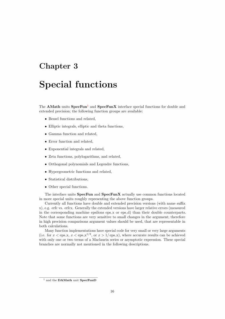
The AMath units SpecFun1 and SpecFunX interface special functions for double andextended precision; the following function groups are available:

• Bessel functions and related,

• Elliptic integrals, elliptic and theta functions,

• Gamma function and related,

• Error function and related,

• Exponential integrals and related,

• Zeta functions, polylogarithms, and related,

• Orthogonal polynomials and Legendre functions,

• Hypergeometric functions and related,

• Statistical distributions,

• Other special functions.

The interface units SpecFun and SpecFunX actually use common functions locatedin more special units roughly representing the above function groups.

Currently all functions have double and extended precision versions (with name suffixx), e.g. erfc vs. erfcx. Generally the extended versions have larger relative errors (measuredin the corresponding machine epsilons eps x or eps d) than their double counterparts.Note that some functions are very sensitive to small changes in the argument; thereforein high precision comparisons argument values should be used, that are representable inboth calculations.

Many function implementations have special code for very small or very large arguments(i.e. for x < eps x, x < eps x1/2, or x > 1/ eps x), where accurate results can be achievedwith only one or two terms of a Maclaurin series or asymptotic expression. These specialbranches are normally not mentioned in the following descriptions.

1 and the DAMath unit SpecFunD

16

3.1 Bessel functions and related

The unit sfBessel contains the common code for the Bessel and related functions.Note that the Bessel functions Jν(x), Yν(x) and some other related functions have an

infinite number of irrational real roots. Except in special cases the AMath functions canhave large relative errors for arguments x near these zeros and only absolute accuracy isachievable; generally the absolute errors have magnitudes of a few eps x.

3.1.1 Bessel functions of integer order

There are some internal routines for the Bessel functions of integer order:

procedure bess_m0p0 (x : extended ; var m0 , p0 : extended ) ;

The procedure returns the modulus M0(x) and phase θ0(x) of J0(x) and Y0(x), for |x| ≥ 9(cf. Abramowitz and Stegun [1, 9.2.17 – 9.2.31]), the results are computed with tworational approximations from Cephes [7, file j0l.c].

procedure bess_m1p1 (x : extended ; var m1 , p1 : extended ) ;

The procedure returns the modulus M1(x) and phase θ1(x) of J1(x) and Y1(x), for |x| ≥ 9(cf. Abramowitz and Stegun [1, 9.2.17 – 9.2.31]), the results are computed with tworational approximations from Cephes [7, file j1l.c].

3.1.1.1 J0(x)

function bessel_j0 (x : double ) : double ;function bessel_j0x (x : extended ) : extended ;

These functions return J0(x), the Bessel function of the 1st kind, order zero. If |x| < 9 arational approximation from Cephes [7, file j0l.c] is used, for 9 ≤ |x| < 500 the commonfunction calls bess m0p0 and returns J0(x) = M0 cos θ0, otherwise the result is computedwith the internal asymptotic function for the real order bessj large(0, x).

3.1.1.2 J1(x)

function bessel_j1 (x : double ) : double ;function bessel_j1x (x : extended ) : extended ;

These functions return J1(x), the Bessel function of the 1st kind, order one. If |x| < 9 arational approximation from Cephes [7, file j1l.c] is used, for 9 ≤ |x| < 500 the commonfunction calls bess m1p1 and returns J1(x) = M1 cos θ1, otherwise the result is computedwith the internal asymptotic function for the real order bessj large(1, x).

3.1.1.3 Jn(x)

function bessel_jn (n : integer ; x : double ) : double ;function bessel_jnx (n : integer ; x : extended ) : extended ;

These functions return Jn(x), the Bessel function of the 1st kind, order n:

Jn(x) = ( 12x)

n∞∑

k=0

(−1)k ( 14x

2)k

k!(n+ k)!, J−n(x) = (−1)nJn(x),

see [30, 10.2.2]. Note: This routine is not suitable for large n or x, in these cases the realorder function Jν(x) with ν = n should be called. For n = 0, 1 the basic functions J0(x)

17

or J1(x) are returned. For x > n the forward recurrence formula

Jn+1(x) =2nxJn(x)− Jn−1(x)

is stable and the result is calculated with the starting values J0(x) and J1(x). For n ≥ xthe formula is unstable and the recurrence is applied in the backward direction. Startingwith Jn+1(x)/Jn(x), which is computed by a continued fraction algorithm2 (3.1), the finalresult is normalized with the value of J0(x).

3.1.1.4 Y0(x)

function bessel_y0 (x : double ) : double ;function bessel_y0x (x : extended ) : extended ;

These functions return Y0(x), the Bessel function of the 2nd kind, order zero for x > 0. Ifx < 9 two rational approximations from Cephes [7, file j0l.c] are used, for 9 ≤ x < 1600the common function calls bess m0p0 and returns Y0(x) = M0 sin θ0, otherwise the resultis computed with the internal asymptotic function for the real order bessy large(0, x).

3.1.1.5 Y1(x)

function bessel_y1 (x : double ) : double ;function bessel_y1x (x : extended ) : extended ;

These functions return Y1(x), the Bessel function of the 2nd kind, order one for x > 0. Ifx < 9 two rational approximations from Cephes [7, file j1l.c] are used, for 9 ≤ x < 1600the common function calls bess m1p1 and returns Y1(x) = M1 sin θ1, otherwise the resultis computed with the internal asymptotic function for the real order bessy large(1, x).

3.1.1.6 Yn(x)

function bessel_yn (n : integer ; x : double ) : double ;function bessel_ynx (n : integer ; x : extended ) : extended ;

These functions return Yn(x), the Bessel function of the 2nd kind, order n for x > 0,expressible for n ≥ 0 as (see [30, 10.8.1]):

Yn(x) = −( 12x)

−n

π

n−1∑k=0

(n− k − 1)!k!

( 14x

2)k +2π

ln( 12x)Jn(x)

−( 12x)

n

π

∞∑k=0

(ψ(k + 1) + ψ(n+ k + 1))(− 1

4x2)k

k!(n+ k)!

and with Y−n(x) = (−1)nYn(x) for negative n. Note: This routine is not suitable forlarge n or x, in these cases the real order function Yν(x) with ν = n should be called. Forn = 0, 1 the basic functions Y0(x) or Y1(x) are returned.

The forward recurrence formula is stable

Yn+1(x) =2nxYn(x)− Yn−1(x)

and is used to compute the result with the starting values Y0(x) and Y1(x).

2 See Press et al.[13, Ch. 5.5 and 6.5] for basic information.

18

3.1.2 Modified Bessel functions of integer order

All of the four basic modified Bessel functions of integer order I0, I1,K0,K1 have internalversions for small arguments.

function bess_i0_small (x : extended ) : extended ;

This routine computes the modified Bessel function I0(x) for |x| ≤ 3 using a Chebyshevapproximation from Fullerton [20, 14] (files dbesi0.f and dbsi0e.f).

function bess_i1_small (x : extended ) : extended ;

This routine computes the modified Bessel function I1(x) for |x| ≤ 3 using a Chebyshevapproximation from Fullerton [20, 14] (files dbesi1.f and dbsi1e.f).

function bess_k0_small (x : extended ) : extended ;

This routine computes the modified Bessel function K0(x) for 0 < x ≤ 2 using a Chebyshevapproximation from Fullerton [20, 14] (files dbesk0.f and dbsk0e.f).

function bess_k1_small (x : extended ) : extended ;

This routine computes the modified Bessel function K1(x) for 0 < x ≤ 2 using a Chebyshevapproximation from Fullerton [20, 14] (files dbesk1.f and dbsk1e.f).

3.1.2.1 I0(x)

function bessel_i0 (x : double ) : double ;function bessel_i0x (x : extended ) : extended ;

These functions compute I0(x), the modified Bessel function of the 1st kind, order 0. If|x| ≤ 3 the result is bess i0 small(x), otherwise e|x|I0,e(x) is returned.

3.1.2.2 Exponentially scaled I0,e(x)

function bessel_i0e (x : double ) : double ;function bessel_i0ex (x : extended ) : extended ;

These functions compute I0,e(x) = e−|x|I0(x), the exponentially scaled modified Besselfunction of the 1st kind, order 0. If |x| ≤ 3 the result is bess i0 small(x)e−|x|, otherwisetwo Chebyshev approximations from Fullerton [20, 14] (file dbsi0e.f) are used.

3.1.2.3 I1(x)

function bessel_i1 (x : double ) : double ;function bessel_i1x (x : extended ) : extended ;

These functions compute I1(x), the modified Bessel function of the 1st kind, order 1. If|x| ≤ 3 the result is bess i1 small(x), otherwise e|x|I1,e(x) is returned.

3.1.2.4 Exponentially scaled I1,e(x)

function bessel_i1e (x : double ) : double ;function bessel_i1ex (x : extended ) : extended ;

These functions compute I1,e(x) = e−|x|I1(x), the exponentially scaled modified Besselfunction of the 1st kind, order 1. If |x| ≤ 3 the result is bess i1 small(x)e−|x|, otherwisetwo Chebyshev approximations from Fullerton [20, 14] (file dbsi1e.f) are used.

19

3.1.2.5 In(x)

function bessel_in (n : integer ; x : double ) : double ;function bessel_inx (n : integer ; x : extended ) : extended ;

These functions calculate In(x), the modified Bessel function of the 1st kind, order n, seee.g. Olver et al. [30, 10.25.2]:

In(x) = ( 12x)

n∞∑

k=0

( 14x

2)k

k!(n+ k)!, In(−x) = (−1)nIn(x), I−n(x) = In(x).

For n = 0, 1 the basic functions I0(x) or I1(x) are returned. For 0 ≤ x ≤ 2 the powerseries is evaluated, otherwise the backward recurrence is used

In−1(x) =2nxIn(x) + In+1(x).

Starting values are computed from the continued fraction (3.2) with ν = n; the final resultis normalized with the value of I0(x).

3.1.2.6 K0(x)

function bessel_k0 (x : double ) : double ;function bessel_k0x (x : extended ) : extended ;

These functions calculate K0(x), the modified Bessel function of the 2nd kind, order zero,x > 0. If x ≤ 2 the result is bess k0 small(x), otherwise e−xK0,e(x) is returned.

3.1.2.7 Exponentially scaled K0,e(x)

function bessel_k0e (x : double ) : double ;function bessel_k0ex (x : extended ) : extended ;

These functions compute K0,e(x) = exK0(x), the exponentially scaled modified Besselfunction of the 2nd kind, order 0, x > 0. If x ≤ 2 the common function returnsbess k0 small(x)ex, otherwise two Chebyshev approximations from Fullerton [20, 14](file dbsk0e.f) are used.

3.1.2.8 K1(x)

function bessel_k1 (x : double ) : double ;function bessel_k1x (x : extended ) : extended ;

These functions calculate K1(x), the modified Bessel function of the 2nd kind, order one,x > 0. If x ≤ 2 the result is bess k1 small(x), otherwise e−xK1,e(x) is returned.

3.1.2.9 Exponentially scaled K1,e(x)

function bessel_k1e (x : double ) : double ;function bessel_k1ex (x : extended ) : extended ;

These functions compute K1,e(x) = exK1(x), the exponentially scaled modified Besselfunction of the 2nd kind, order one, x > 0. If x ≤ 2 the common function returnsbess k1 small(x)ex, otherwise two Chebyshev approximations from Fullerton [20, 14] (filedbsk1e.f) are used.

20

3.1.2.10 Kn(x)

function bessel_kn (n : integer ; x : double ) : double ;function bessel_knx (n : integer ; x : extended ) : extended ;

These functions return Kn(x), the modified Bessel function of the 2nd kind, order n forx > 0, expressible for n ≥ 0 as (see [30, 10.31.1]):

Kn(x) = 12 ( 1

2x)−n

n−1∑k=0

(n− k − 1)!k!

(− 14x

2)k + (−1)n+1 ln( 12x)In(x)

+ (−1)n+1 12 ( 1

2x)n∞∑

k=0

(ψ(k + 1) + ψ(n+ k + 1))( 14x

2)k

k!(n+ k)!

and with K−n(x) = Kn(x) for negative n. Note: This routine is not suitable for large nor x, in these cases the real order function Kν(x) with ν = n should be called. For n = 0, 1the basic functions K0(x) or K1(x) are returned. The forward recurrence formula is stable

Kn+1(x) =2nxKn(x) +Kn−1(x)

and is used to compute the result with the starting values K0(x) and K1(x).

3.1.3 Bessel functions of real order

First the internal functions are described; ν is written as v in the source code.

procedure h1v_large (v , x : extended ; var mv , tmx : extended ) ;

The procedure calculates the modulus Mν(x) and phase θν(x) of the Hankel functionH

(1)ν (x) = Jν(x)+iYν(x) for large x > 0 using the asymptotic expansions from Abramowitz

and Stegun [1, 9.2.28/9.2.29] with µ = 4ν2 :

M2ν ∼

2πx

(1 +

12µ− 1(2x)2

+1 · 32 · 4

(µ− 1)(µ− 9)(2x)4

+1 · 3 · 52 · 4 · 6

(µ− 1)(µ− 9)(µ− 25)(2x)6

· · ·)

θν ∼ x− ( 12ν + 1

4 )π +µ− 12(4x)

+(µ− 1)(µ− 25)

6(4x)3+

(µ− 1)(µ2 − 114µ+ 1073)5(4x)5

· · ·

The returned values are mv = Mν(x) and tmx = θν(x)− x.

function bessj_large (v , x : extended ) : extended ;

This function returns Jν(x) for large x > 0 with the modulus/phase asymptotic expansionh1v large and Jν(x) = Mν cos θν .

function bessy_large (v , x : extended ) : extended ;

This function returns Yν(x) for large x > 0 with the modulus/phase asymptotic expansionh1v large and Yν(x) = Mν sin θν .

procedure bessel_jy (v , x : extended ; BT : byte ; var Jv , Yv : extended ) ;

This procedure returns Jν(x) and/or Yν(x) depending on BT, it assumes x > 0 and|ν| < MaxLongint. (For x < 0 the functions Jν and Yν are in general complex; and Yν issingular for x = 0.)

bessel jy is a bit complicated and this description shows only the main implementationtopics, for the subtle parts the source code is the final reference.

21

If x is ’large’ (this depends on ν), the asymptotic expansions are used, and for ν < 0the functions are computed with the reflection formulas [13, 6.7.19]

J−ν(x) = cos(πν)Jν(x)− sin(πν)Yν(x),Y−ν(x) = sin(πν)Jν(x) + cos(πν)Yν(x).

The essential calculation method is described in Ch. 6.7 and the C function bessjyin Press et al.[13], some ideas are from the Boost [19] code in file bessel jy.hpp, functionbessel jy. Steed’s method for x ≥ 2 uses two continued fractions and the Wronskian relation

Jν(x)Y ′ν(x)− Yν(x)J ′ν(x) =2πx

to compute Jν , J ′ν , Yν , and Y ′ν simultaneously. The first continued fraction CF1 ([13, 6.7.2]and [1, 9.1.73]) evaluates

J ′νJν

=ν

x− Jν+1

Jν=ν

x− 1

2(ν + 1)/x −1

2(ν + 2)/x −· · · (3.1)

while the second CF2 from [13, 6.7.3] is complex

J ′ν + iY ′νJν + iYν

= − 12x

+ i+i

x

(1/2)2 − ν2

2(x+ i) +(2/2)2 − ν2

2(x+ 2i) +· · ·

If x < 2 Temme’s method [51] for evaluating Yν′ and Yν′+1 (with |ν′| ≤ 1/2) is usedtogether with the forward recurrence relation to get Yν(x). If Jν(x) is needed, it iscomputed with CF1 and the Wronskian.

3.1.3.1 Jν(x)

function bessel_jv (v , x : double ) : double ;function bessel_jvx (v , x : extended ) : extended ;

These functions return Jν(x), the Bessel function of the 1st kind, real order ν:

Jν(x) = ( 12x)

ν∞∑

k=0

(−1)k ( 14x

2)k

k!Γ(ν + k + 1),

see [30, 10.2.2], if x < 0 then ν must be an integer. The formula is used only for x < 1 orν > x2/4. If ν = n is an integer smaller than 200 then Jn(x) is returned. Otherwise theresult is computed with general procedure bessel jy.

3.1.3.2 Yν(x)

function bessel_yv (v , x : double ) : double ;function bessel_yvx (v , x : extended ) : extended ;

These functions return Yν(x), the Bessel function of the 2nd kind, real order ν, and x > 0;see [30, 10.2.3]:

Yν(x) =Jν(x) cos(νπ)− J−ν(x)

sin(νπ).

The result is computed with general procedure bessel jy, except in two special cases: Whenν = n is an integer smaller than 2000 then Yn(x) is returned, and if ν is a negativehalf-integer then Yν(x) = −J−ν(x) sin νπ (this may avoid the reflection formulas with bothfunctions, note | sin νπ| = 1 in this case).

22

3.1.3.3 Bessel Λν(x)

function bessel_lamda (v , x : double ) : double ;function bessel_lamdax (v , x : extended ) : extended ;

These functions return for x, ν ≥ 0 the Bessel Λν(x) function, defined by3

Λν(x) = Γ(ν + 1)Jν(x)(x/2)ν

=∞∑

k=0

(− 14x

2)k

k!(1 + ν)k

For x ≤ 0.002 the result is the sum of the first 3 terms, otherwise Jν is used.

3.1.4 Modified Bessel functions of real order

The internal functions are described first, they are similar to the unmodified.

procedure bessel_ik (v , x : extended ; CalcI , escale : boolean ;var Iv , Kv : extended ) ;

This procedure returns Iν(x) and/or Kν(x) depending on CalcI for x > 0, and |ν| <MaxLongint. If escale=true the values are exponentially scaled. For ν < 0 the functionsare computed with the reflection formulas [13, 6.7.40]

I−ν(x) = Iν(x) +2π

sin(πν)Kν(x),

K−ν(x) = Kν(x).

The Wronskian relation for the modified functions is ([13, 6.7.20])

Iν(x)K ′ν(x)−Kν(x)I ′ν(x) = − 1

x,

and the first continued fraction CF1 becomes (see [13, 6.7.21] and [30, 10.33.1]):

Iν+1

Iν=I ′νIν− ν

x=

12(ν + 1)/x+

12(ν + 2)/x +

· · · (3.2)

CF2 is a bit complicated and described in [13, 6.7.22–6.7.27].The forward recurrence for Kν is used, if x < 2 with a corresponding Temme normali-

sation [52] or CF2 otherwise.When Iν(x) shall be computed, this is done with an asymptotic expansion from [1,

9.7.1] or [30, 10.40.4] if x > 100 and 2ν < x1/2; otherwise CF1 and the Wronskian areused.

3.1.4.1 Iν(x)

function bessel_iv (v , x : double ) : double ;function bessel_ivx (v , x : extended ) : extended ;

These functions return Iν(x), the modified Bessel function of the 1st kind, real order ν,x ≥ 0 if ν is not an integer, defined as [30, 10.25.2]:

Iν(x) = ( 12x)

ν∞∑

k=0

( 14x

2)k

k!Γ(ν + k + 1)

3 See http://mathworld.wolfram.com/LambdaFunction.html

23

The common routine sfc iv handles the four special ν cases

Iν(x) =

I0(x) ν = 0,I1(x) |ν| = 1,sinh(x)/(xπ/2)1/2 ν = 1/2,cosh(x)/(xπ/2)1/2 ν = −1/2.

For other arguments the general procedure bessel ik is used.

3.1.4.2 Exponentially scaled Iν,e(x)

function bessel_ive (v , x : double ) : double ;function bessel_ivex (v , x : extended ) : extended ;

The functions return Iν,e(x) = Iν(x) exp(−|x|) the exponentially scaled modified Besselfunction of the 1st kind, real order ν, x ≥ 0 if ν is not an integer. When ν = 0 or |ν| = 1the integer order routines I0,e(x) or I1,e(x) are used, otherwise the result is computedwith the general procedure bessel ik.

3.1.4.3 Kν(x)

function bessel_kv (v , x : double ) : double ;function bessel_kvx (v , x : extended ) : extended ;

These functions return Kν(x), the modified Bessel function of the 2nd kind, real order ν,x > 0, defined as [30, 10.27.4]:

Kν(x) =π

2I−ν(x)− Iν(x)

sin(νπ)

If ν = n is an integer4 the integer order function Kn is used. For |ν| = 1/2 there is thespecial case exp(−x)(π/(2x))1/2, and otherwise the result is computed with the generalprocedure bessel ik.

3.1.4.4 Exponentially scaled Kν,e(x)

function bessel_kve (v , x : double ) : double ;function bessel_kvex (v , x : extended ) : extended ;

These functions return exKν(x), the exponentially scaled modified Bessel function of the2nd kind, real order ν, x > 0. When ν = 0 or |ν| = 1 the integer order routines K0,e(x) orK1,e(x) are used, for |ν| = 1/2 the value (π/(2x))1/2 is returned, otherwise the result iscomputed with the general procedure bessel ik.

3.1.5 Airy functions

In this section let z = (2/3)|x|3/2. For large negative x the Airy functions and the Scorerfunction Gi(x) have asymptotic expansions oscillating with cos(z + π/4) or sin(z + π/4),see Abramowitz and Stegun [1, 10.4.60, 10.4.64, 10.4.87]; therefore the phase informationbecomes totally unreliable for x < −(2/eps x)2/3 ≈ −0.7E13, and the relative errorincreases strongly for x less than the square root (≈ −2.6E6).

4 and less than MaxLongint

24

For x ≥ 0 the Airy functions can be defined by

Ai(x) =1π

√x

3K1/3(z),

Bi(x) =√x

3(I1/3(z) + I−1/3(z)

).

There are two parametrised internal functions that compute the Airy functions for smallarguments:

function Airy_small (x , f0 , f1 : extended ) : extended ;

This function returns Ai(x) or Bi(x) using Maclaurin series for ’small’ x. It evaluates thetwo series expansions from Olver et al. [30, 9.4.1/9.4.3]:

f0 ·(1 +

13!x3 +

1 · 46!

x6 +1 · 4 · 7

9!x9 + · · ·

)+ f1 ·

(x+

24!x4 +

2 · 57!

x7 +2 · 5 · 8

10!x10 + · · ·

)function AiryP_small (x , f0 , f1 : extended ) : extended ;

This function returns Ai′(x) or Bi′(x) using Maclaurin series for ’small’ x. It evaluates thetwo series expansions from Olver et al. [30, 9.4.2/9.4.4]:

f0 ·(1 +

23!x3 +

2 · 56!

x6 +2 · 5 · 8

9!x9 + · · ·

)+ f1 ·

( 12!x2 +

1 · 45!

x5 +1 · 4 · 7

8!x8 + · · ·

)3.1.5.1 Airy Ai(x)

function airy_ai (x : double ) : double ;function airy_aix (x : extended ) : extended ;

These functions calculate the Airy function Ai(x). Airy small(x, f0, f1) is returned for−2 ≤ x ≤ 1 with

f0 = Ai(0) = 3−2/3/Γ(2/3), f1 = Ai′(0) = −3−1/3/Γ(1/3).

For x > 1 the definition formula is evaluated

Ai(x) =1π

√x

3K1/3(z),

and for x < −2 the result is (cf. Press et al. [13, 6.7.46]):

Ai(x) = 12

√−x(J1/3(z)−

1√3Y1/3(z)

).

3.1.5.2 Airy Bi(x)

function airy_bi (x : double ) : double ;function airy_bix (x : extended ) : extended ;

These functions calculate the Airy function Bi(x). Airy small(x, f0, f1) is returned for−1 ≤ x ≤ 1 with

f0 = Bi(0) = 3−1/6/Γ(2/3), f1 = Bi′(0) = 31/6/Γ(1/3).

For x > 1 the formula from [13, 6.7.44] is used

Bi(x) =√x

(2√3I1/3(z) +

1πK1/3(z)

),

and for x < −1 the result is [13, 6.7.46]:

Bi(x) = − 12

√−x(

1√3J1/3(z) + Y1/3(z)

).

25

3.1.5.3 Airy Ai’(x)

function airy_aip (x : double ) : double ;function airy_aipx (x : extended ) : extended ;

These functions calculate the Airy function Ai′(x). AiryP small(x,Ai(0),Ai′(0)) is re-turned if −1 ≤ x ≤ 1. For x > 1 the formula from [13, 6.7.45] is used

Ai′(x) = − x

π√

3K2/3(z),

and for x < −1 the result is [13, 6.7.46]):

Ai′(x) = −x2

(J2/3(z) +

1√3Y2/3(z)

).

3.1.5.4 Airy Bi’(x)

function airy_bip (x : double ) : double ;function airy_bipx (x : extended ) : extended ;

These functions calculate the Airy function Bi′(x). AiryP small(x,Bi(0),Bi′(0)) is returnedif −1 ≤ x ≤ 1. For x > 1 the formula from [13, 6.7.45] is used

Bi′(x) = x

(2√3I2/3(z) +

1πK2/3(z)

),

and for x < −1 the result is [13, 6.7.46]:

Bi′(x) = −x2

(1√3J2/3(z)− Y2/3(z)

).

3.1.5.5 Scaled Airy Ais(x)

function airy_ais (x : double ) : double ;function airy_aisx (x : extended ) : extended ;

These functions return the scaled Airy function Ais(x), defined as Ais(x) = ez Ai(x) forx > 0 and Ais(x) = Ai(x) otherwise. For x ≤ 1 the common function sfc airy ais usesthe definition, if x ≥ 241 the asymptotic expression from [1, 10.4.59]

Ais(x) ∼12π−1/2x−1/4

is evaluated; otherwise bessel ik is called to the get the scaled Bessel functions.

3.1.5.6 Scaled Airy Bis(x)

function airy_bis (x : double ) : double ;function airy_bisx (x : extended ) : extended ;

These functions return the scaled Airy function Bis(x), defined as Bis(x) = e−z Bi(x) forx > 0 and Bis(x) = Bi(x) otherwise. For x ≤ 10−20 the common function sfc airy bisuses Bi(x), if x ≥ 241 the asymptotic expression from [1, 10.4.63]

Bis(x) ∼ π−1/2x−1/4

is evaluated; otherwise bessel ik is called to the get the scaled Bessel functions, wherethe K1/3(z) contribution is negligible if x > 12.

26

3.1.5.7 Airy Gi(x)

function airy_gi (x : double ) : double ;function airy_gix (x : extended ) : extended ;

These functions calculate the inhomogeneous Airy function Gi(x) (also called Scorerfunction), cf. [30, 9.12.19]:

Gi(x) =1π

∫ ∞

0

sin(xt− 1

3t3)

dt

The common function sfc airy gi uses Chebyshev approximations from MacLeod’sMISCFUN [22, function AIRYGI], and sfc airy bi instead of the in-line approximationsfor Bi(x).

3.1.5.8 Airy Hi(x)

function airy_hi (x : double ) : double ;function airy_hix (x : extended ) : extended ;

These functions calculate the inhomogeneous Airy function Hi(x) (also called Scorerfunction), cf. [30, 9.12.20]:

Hi(x) =1π

∫ ∞

0

exp(xt− 1

3t3)

dt

The common function sfc airy hi uses Chebyshev approximations from MacLeod’sMISCFUN [22, function AIRYHI], and sfc airy bi instead of the in-line approximationsfor Bi(x).

3.1.6 Kelvin functions

The Kelvin functions of general order ν can be defined as

berν(x) + ibeiν(x) = e+νπi/2Iν(xeπi/4)

kerν(x) + i keiν(x) = e−νπi/2Kν(xeπi/4)

see Abramowitz and Stegun [1, 9.9.1 and 9.9.2]. When ν = 0, suffices and brackets arenormally suppressed. These definitions show that the four functions ber, bei, ker, andkei are tightly related, e.g. in the implemented asymptotic expansion for say ber all fourfunctions are computed. Consequently there are some internal routines common to theKelvin functions:

function ber_sm (x : extended ) : extended ;

This function computes the Kelvin function berx = ber0(x) for 0 ≤ x < 20 with the seriesexpansion [1, 9.9.10]:

berx =∞∑

k=0

(−1)k ( 14x

2)2k

((2k)!)2

function bei_sm (x : extended ) : extended ;

This function computes the Kelvin function beix = bei0(x) for 0 ≤ x < 20 with the seriesexpansion [1, 9.9.10]:

beix =∞∑

k=0

(−1)k ( 14x

2)2k+1

((2k + 1)!)2

27

function ker_sm (x : extended ) : extended ;

This function computes the Kelvin function kerx = ker0(x) for 0 < x < 3 with the seriesexpansion [1, 9.9.12]:

kerx = − ln( 12x) berx+ 1

4π beix+∞∑

k=0

(−1)k ψ(2k + 1)((2k)!)2

( 14x

2)2k

or with the harmonic numbers Hk = ψ(k + 1) + γ

kerx = −(γ + ln( 12x)) berx+ 1

4π beix+∞∑

k=0

(−1)k H2k

((2k)!)2( 14x

2)2k

function kei_sm (x : extended ) : extended ;

This function computes the Kelvin function keix = kei0(x) for 0 < x < 3 with the seriesexpansion [1, 9.9.12]:

keix = − ln( 12x) beix− 1

4π berx+∞∑

k=0

(−1)k ψ(2k + 2)((2k + 1)!)2

( 14x

2)2k+1

= −(γ + ln( 12x)) beix− 1

4π berx+∞∑

k=0

(−1)k H2k+1

((2k + 1)!)2( 14x

2)2k+1

procedure kelvin_large (x : extended ; cb : boolean ;var br , bi , kr , ki : extended ) ;

This procedure computes all four Kelvin functions for x ≥ 20 using asymptotic expansionsfrom [1, 9.10.1 – 9.10.7]:

kerx =√π/(2x)e−x/

√2(

+ f0(−x) cosβ − g0(−x) sinβ),

keix =√π/(2x)e−x/

√2(− f0(−x) sinβ − g0(−x) cosβ

),

berx =ex/

√2

√2πx

(f0(x) cosα+ g0(x) sinα

)− 1π

keix,

beix =ex/

√2

√2πx

(f0(x) sinα− g0(x) cosα

)+

1π

kerx,

with α = x/√

2− 18π and β = α+ 1

4π and the auxiliary functions

f0(±x) ∼ 1 +∞∑

k=1

(∓1)k (−1)(−9) · · · (−(2k − 1)2)k!(8x)k

cos( 14kπ)

g0(±x) ∼ +∞∑

k=1

(∓1)k (−1)(−9) · · · (−(2k − 1)2)k!(8x)k

sin( 14kπ)

ker and kei are always calculated, ber and bei only if cb=true.

procedure ker_kei_med (x : extended ; var kr , ki : extended ) ;

This procedure bridges the gap 3 ≤ x ≤ 20 for ker and kei, basically it uses the asymptoticform but each of the functions f0 and g0 are evaluated with a Chebyshev approximation.

28

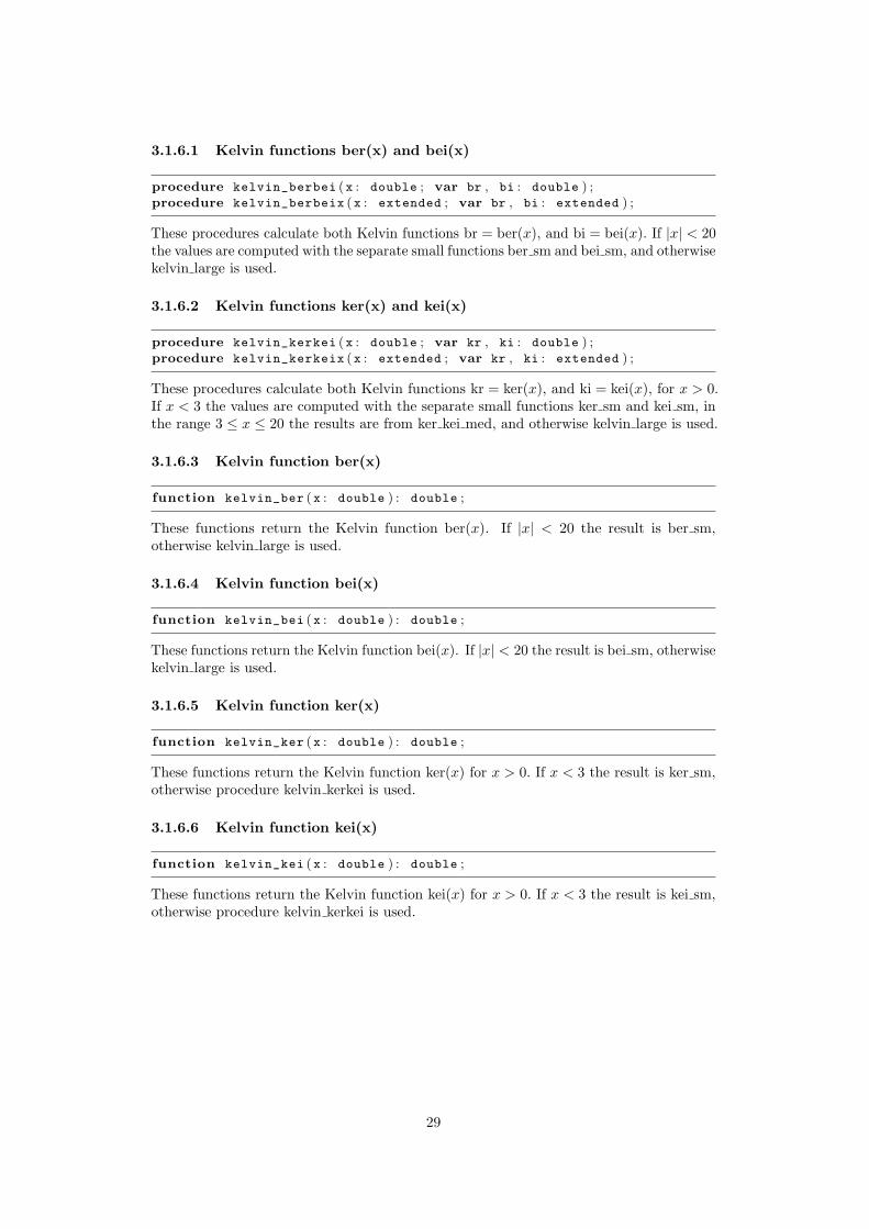
3.1.6.1 Kelvin functions ber(x) and bei(x)

procedure kelvin_berbei (x : double ; var br , bi : double ) ;procedure kelvin_berbeix (x : extended ; var br , bi : extended ) ;

These procedures calculate both Kelvin functions br = ber(x), and bi = bei(x). If |x| < 20the values are computed with the separate small functions ber sm and bei sm, and otherwisekelvin large is used.

3.1.6.2 Kelvin functions ker(x) and kei(x)

procedure kelvin_kerkei (x : double ; var kr , ki : double ) ;procedure kelvin_kerkeix (x : extended ; var kr , ki : extended ) ;

These procedures calculate both Kelvin functions kr = ker(x), and ki = kei(x), for x > 0.If x < 3 the values are computed with the separate small functions ker sm and kei sm, inthe range 3 ≤ x ≤ 20 the results are from ker kei med, and otherwise kelvin large is used.

3.1.6.3 Kelvin function ber(x)

function kelvin_ber (x : double ) : double ;

These functions return the Kelvin function ber(x). If |x| < 20 the result is ber sm,otherwise kelvin large is used.

3.1.6.4 Kelvin function bei(x)

function kelvin_bei (x : double ) : double ;

These functions return the Kelvin function bei(x). If |x| < 20 the result is bei sm, otherwisekelvin large is used.

3.1.6.5 Kelvin function ker(x)

function kelvin_ker (x : double ) : double ;

These functions return the Kelvin function ker(x) for x > 0. If x < 3 the result is ker sm,otherwise procedure kelvin kerkei is used.

3.1.6.6 Kelvin function kei(x)

function kelvin_kei (x : double ) : double ;

These functions return the Kelvin function kei(x) for x > 0. If x < 3 the result is kei sm,otherwise procedure kelvin kerkei is used.

29

3.1.7 Spherical Bessel functions

3.1.7.1 Spherical Bessel function jn(x)

function sph_bessel_jn (n : integer ; x : double ) : double ;function sph_bessel_jnx (n : integer ; x : extended ) : extended ;

These functions return jn(x), the spherical Bessel function of the 1st kind, order n. Exceptfor n = 0 where the value sinc(x) is used, the result is calculated just from the definition[1, 10.1.1]:

jn(x) =√

12π/x Jn+

12(x) (x ≥ 0), and jn(−x) = (−1)njn(x).

3.1.7.2 Spherical Bessel function yn(x)

function sph_bessel_yn (n : integer ; x : double ) : double ;function sph_bessel_ynx (n : integer ; x : extended ) : extended ;

These functions return yn(x), the spherical Bessel function of the 2nd kind, order n, x 6= 0.The result is calculated using the definition [1, 10.1.1]:

yn(x) =√

12π/x Yn+

12(x) (x > 0), and yn(−x) = (−1)n+1yn(x).

3.1.7.3 Modified spherical Bessel function in(x)

function sph_bessel_in (n : integer ; x : double ) : double ;function sph_bessel_inx (n : integer ; x : extended ) : extended ;

These functions compute in(x), the modified spherical Bessel function of the 1st (and2nd) kind, order n. Except for n = 0 where the value sinh(x)/x is returned, the result iscalculated just from the definition [1, 10.2.2] or [30, 10.47.7]

in(x) =√

12π/x In+

12(x) (x ≥ 0), and in(−x) = (−1)nin(x)

with the reflection formula from [30, 10.47.16]. Note that in is named i(1)n in the NIST

handbook [30] and restricted to n ≥ 0, the modified spherical Bessel function of the 2ndkind is then defined as

i(2)n (x) =√

12π/x I−n− 1

2(x),

which can be expressed by in, i.e.

i(1)n (x) = in(x), i(2)n (x) = i−n−1(x), (for n ≥ 0).

3.1.7.4 Exponentially scaled in,e(x)

function sph_bessel_ine (n : integer ; x : double ) : double ;function sph_bessel_inex (n : integer ; x : extended ) : extended ;

These functions return in(x) exp(−|x|), the exponentially scaled modified spherical Besselfunction of the 1st/2nd kind, order n. For n = 0 the result is

i0,e(x) = −expm1(−2|x|)2|x|

,

otherwise the common function sfc sph ine uses Iν,e(x), the exponentially scaled modifiedBessel function of the 1st kind:

in,e(x) =√

12π/x In+

12 ,e

(x) (x ≥ 0), and in,e(−x) = (−1)nin,e(x)

30

3.1.7.5 Modified spherical Bessel function kn(x)

function sph_bessel_kn (n : integer ; x : double ) : double ;function sph_bessel_knx (n : integer ; x : extended ) : extended ;

These functions return kn(x), the modified spherical Bessel function of the 3rd kind, ordern, x > 0. Except for n = 0 the result is calculated just from the definition [30, 10.47.9]:

k0(x) = 12πe−x

xand kn(x) =

√12π/x Kn+

12(x), (x > 0).

3.1.7.6 Exponentially scaled kn,e(x)

function sph_bessel_kne (n : integer ; x : double ) : double ;function sph_bessel_knex (n : integer ; x : extended ) : extended ;

These functions compute kn(x)ex, the exponentially scaled modified spherical Besselfunction of the 3rd kind. For n = 0 the result is π

2x , otherwise the common functionsfc sph kne returns

kn,e(x) =√

12π/x Kn+

12 ,e

(x) (x > 0).

3.1.8 Struve functions

For real ν, x the Struve functions Hν(x) and the modified Struve functions Lν(x) havethe power series expansions (see Abramowitz and Stegun [1, 12.1.3 and 12.2.1])5:

Hν(x) = ( 12x)

ν+1∞∑

k=0

(−1)k( 12x)

2k

Γ(k + 32 )Γ(k + ν + 3

2 )=

2(

12x)ν+1

√πΓ(ν + 3

2 )

∞∑k=0

(−1)k( 12x)

2k(32

)k

(ν + 3

2

)k

Lν(x) = ( 12x)

ν+1∞∑

k=0

( 12x)

2k

Γ(k + 32 )Γ(k + ν + 3

2 )=

2(

12x)ν+1

√πΓ(ν + 3

2 )

∞∑k=0

( 12x)

2k(32

)k

(ν + 3

2

)k

Hν(x) has the asymptotic expansion for large x > 0 [1, 12.1.29]:

Hν(x) ∼ Yν(x) +1π

∞∑k=0

Γ(k + 12 )

Γ(ν + 12 − k)( 1

2x)2k−ν+1

∼ Yν(x) +

(12x)ν−1

√πΓ(ν + 3

2 )

∞∑k=0

( 12 )k( 1

2 − ν)k

(− 4x2

)k

and the integral representation for x > 0 [1, 12.1.8]:

Hν(x) = Yν(x) +2( 1

2x)k

√πΓ(ν + 1

2 )

∫ ∞

0

e−xt(1 + t2)ν− 12 dt

Lν(x) has the asymptotic expansion for large x > 0 [1, 12.2.6]:

Lν(x) ∼ I−ν(x)− 1π

∞∑k=0

(−1)kΓ(k + 12 )

Γ(ν + 12 − k)( 1

2x)2k−ν+1

∼ I−ν(x)−(

12x)ν−1

√πΓ(ν + 3

2 )

∞∑k=0

( 12 )k( 1

2 − ν)k

(4x2

)k

5 For the sums with Pochhammer symbol see http://functions.wolfram.com/03.09.06.0027.01 forHν(x) and http://functions.wolfram.com/03.10.06.0028.01 for Lν(x).

31

3.1.8.1 Struve H0(x)

function struve_h0 (x : double ) : double ;function struve_h0x (x : extended ) : extended ;

These functions calculate H0(x), the Struve function of order 0. For x < 0 the resultis −H0(|x|). The common function sfc struve h0 uses two Chebyshev approximationsfrom [22, function STRVH0], one for x < 11 and the second together with a call to Y0(x)otherwise.6

3.1.8.2 Struve H1(x)

function struve_h1 (x : double ) : double ;function struve_h1x (x : extended ) : extended ;

These functions calculate H1(x), the Struve function of order 1. The common functionsfc struve h1 uses two Chebyshev approximations from [22, function STRVH1], one for|x| < 9 and the second together with a call to Y1(x) otherwise.

3.1.8.3 Struve function Hν(x)

function struve_h (v , x : double ) : double ;function struve_hx (v , x : extended ) : extended ;

These functions compute Hν(x), the Struve function of order ν7. Negative x are allowedonly for integer ν = n and then the reflection formula Hn(−x) = (−1)n+1Hn(x) is applied.

When ν = 0, 1 the basic functions H0(x) or H1(x) are returned and for negativehalf-integers H−n− 1

2(x) = Y−n− 1

2(x). For ν = 1

2 there is the special case [1, 12.1.16]:

H 12(x) =

(2πx

) 12

(1− cosx) =versx√xπ/2

The order ν = 12 is a border case: For ν > 1

2 the functions Hν(x) have no zero other thanx = 0, but when ν ≤ 1

2 there are an infinite number of irrational real roots8. And nearthese zeros only absolute accuracy is achievable, i.e. the AMath functions may have largerelative errors.

For x ≥ 0 the common function sfc struve h evaluates the power series for small x andthe asymptotic expansion for large x; in the medium range9 the integral representation isused with a custom version of the double-exponential integration routine from AMTools.

3.1.8.4 Modified Struve function Lν(x)

function struve_l (v , x : double ) : double ;function struve_lx (v , x : extended ) : extended ;

These functions return Lν(x), the modified Struve function of order ν. Negative x areallowed only for integer ν = n where the formula Ln(−x) = (−1)n+1Ln(x) is used.

6 The function in [22] has a third approximation instead of Y0.7 ν is written as v in the source code.8 Asymptotically for large x the functions look like a damped sin : Hν(x) ∼

q2

πxsin(x− (2ν + 1)π/4);

see http://functions.wolfram.com/03.09.06.0041.01 ff.9 The three ranges depend on x and ν.

32

For negative half-integers there is the relation L−n− 12(x) = In+ 1

2(x); the special cases

Lν(0) = 0, ν > −1, and ν = 12 (see [30, 11.4.7])

L 12(x) =

(2πx

) 12

(coshx− 1)

are handled separately, otherwise the common function sfc struve l evaluates the powerseries for small and medium x and the asymptotic expansion for large x.

3.1.8.5 Struve L0(x)

function struve_l0 (x : double ) : double ;function struve_l0x (x : extended ) : extended ;

These legacy routines return the Struve function L0(x), in the current implementationthey just call sfc struve l(0,x).

3.1.8.6 Struve L1(x)

function struve_l1 (x : double ) : double ;function struve_l1x (x : extended ) : extended ;

These legacy routines return the Struve function L1(x), in the current implementationthey just call sfc struve l(1,x).

33

3.2 Elliptic integrals, elliptic and theta functions

The Pascal unit sfEllInt implements the common code for the elliptic integrals, ellipticand theta functions.

3.2.1 Legendre style elliptic integrals

3.2.1.1 Complete elliptic integral of the 1st kind

function comp_ellint_1 (k : double ) : double ;function comp_ellint_1x (k : extended ) : extended ;

These functions compute the value of the complete elliptic integral of the first kind K(k)and the real part if |k| > 1.

K(k) =∫ π/2

0

dt√1− k2 sin2 t

.

The common function sfc EllipticK returns

K(k) =π/2

agm(1,√

1− k2),

where the AGM is performed in-line, see 3.10.1 for the algorithm. For |k| > 1 the firstformula of [30, 19.7.3] is used to to get <K(k) = K(1/k)/k.

3.2.1.2 Complete elliptic integral of the 2nd kind

function comp_ellint_2 (k : double ) : double ;function comp_ellint_2x (k : extended ) : extended ;

These functions compute the value of the complete elliptic integral of the second kind E(k)and the real part if |k| > 1.

E(k) =∫ π/2

0

√1− k2 sin2 t dt .

The common function sfc EllipticEC returns

E(k) = cel2(kc, 1, k2c )

For |k| > 1 the third formula of [30, 19.7.3] gives (with 3.2.1.4)

<E(1/k) = (1/k)(E(k)− k2

cK(k))

= kB(k) =⇒ <E(k) = B(1/k)/k

3.2.1.3 Complete elliptic integral of the 3rd kind

function comp_ellint_3 (nu , k : double ) : double ;function comp_ellint_3x (nu , k : extended ) : extended ;

These functions compute the value of the complete elliptic integral of the third kind Π(ν, k)with modulus |k| < 1, and parameter ν 6= 1

Π(ν, k) =∫ π/2

0

dt

(1− ν sin2 t)√

1− k2 sin2 t.

The common function sfc EllipticPiC returns

Π(ν, k) = cel(kc, 1− ν, 1, 1)

with kc =√

1− k2, cf. Bulirsch[11, 1.2.2].

34

3.2.1.4 Complete elliptic integral B(k)

function comp_ellint_b (k : double ) : double ;function comp_ellint_bx (k : extended ) : extended ;

These functions compute the value of the complete Legendre style elliptic integral B(k)with modulus |k| ≤ 1 :

B(k) =∫ π/2

0

cos2 t dt√1− k2 sin2 t

=E(k)− k2

cK(k)k2

.

For |k| < 2 · 10−5 two terms of the Maclaurin expansion computed with Maple are used

B(k) =14π

(1 +

18k2 +

364k4 +O(k6)

),

otherwise the common function sfc cel b returns

B(k) = cel2(kc, 1, 0)

with kc =√

1− k2, cf. Bulirsch[10, p.80].

3.2.1.5 Complete elliptic integral D(k)

function comp_ellint_d (k : double ) : double ;function comp_ellint_dx (k : extended ) : extended ;

These functions compute the value of the complete Legendre style elliptic integral D(k)with modulus |k| < 1 :

D(k) =∫ π/2

0

sin2 t dt√1− k2 sin2 t

=K(k)− E(k)

k2.

For |k| < 2 · 10−5 two terms of the Maclaurin expansion [30, 19.5.3] are used

D(k) =14π

(1 +

38k2 +

1564k4 +O(k6)

),

otherwise the common function sfc cel d returns

D(k) = cel2(kc, 0, 1)

with kc =√

1− k2, cf. Bulirsch[10, p.80].

3.2.1.6 Legendre elliptic integral of the 1st kind

function ellint_1 ( phi , k : double ) : double ;function ellint_1x ( phi , k : extended ) : extended ;

These functions compute the incomplete Legendre elliptic integral of the first kind

F (ϕ, k) =∫ ϕ

0

dt√1− k2 sin2 t

with |k sinϕ| ≤ 1. Obviously F (ϕ, k) = ϕ for k = 0; and if |k| = 1 and |ϕ| < π/2 thenF (ϕ, k) = arcgdϕ (see [30, 19.6.8]).

35

If |k| > 1 the common function sfc ellint 1 performs a reciprocal-modulus transfor-mation [30, 19.7.4]

F (ϕ, k) = F (arcsin(k sinϕ), 1/k) /k

= el1(tan (arcsin(k sinϕ)) , (1− 1/k2)1/2

)/k.

For |k| < 1 the argument ϕ is reduced mod π, i.e. ϕ = nπ + ϕ′ with |ϕ′| ≤ π/2. If|ϕ′| = π/2, i.e. ϕ is an odd multiple m of π/2, then F = mK(k). For |ϕ′| < π/2 theintegral is calculated with Bulirsch’s [10] el1:

F (ϕ, k) = el1(tanϕ′,√

1− k2).

And since F is quasi-periodic10 the total result is

F (ϕ, k) = 2nK(k) + el1(tanϕ′,√

1− k2).

3.2.1.7 Legendre elliptic integral of the 2nd kind

function ellint_2 ( phi , k : double ) : double ;function ellint_2x ( phi , k : extended ) : extended ;

These functions compute the incomplete Legendre elliptic integral of the second kind

E(ϕ, k) =∫ ϕ

0

√1− k2 sin2 t dt

with |k sinϕ| ≤ 1. Again E(ϕ, k) = ϕ for k = 0. If |k| > 1 the common functionsfc ellint 2 performs a reciprocal-modulus transformation [30, 19.7.4]. The right handside R(β, k) = (E(β, k) − k′2F (β, k))/k with k sinβ = sinϕ can be rewritten with thefunction

B(β, k) =∫ β

0

cos2 x(1− k2 sin2 x)1/2

dx

as R = kB(β, k). The B integral can be evaluated by a single call to the function el2 (orcel2 if β = π/2), see Bulirsch [10].

For |k| < 1 the argument ϕ is reduced mod π, i.e. ϕ = nπ + ϕ′ with |ϕ′| ≤ π/2. If|ϕ′| = π/2, i.e. ϕ is an odd multiple m of π/2, then E(ϕ, k) = mE(k). For |ϕ′| < π/2 theintegral is calculated with Bulirsch’s [10] el2:

E(ϕ, k) = el2(tanϕ′, kc, 1, k2c ), k2

c = 1− k2.

And since E(ϕ, k) is quasi-periodic the total result is

E(ϕ, k) = 2nE(k) + el2(tanϕ′, kc, 1, k2c ).

3.2.1.8 Legendre elliptic integral of the 3rd kind

function ellint_3 ( phi , nu , k : double ) : double ;function ellint_3x ( phi , nu , k : extended ) : extended ;

These functions compute the incomplete Legendre elliptic integral of the third kind

Π(ϕ, ν, k) =∫ ϕ

0

dt

(1− ν sin2 t)√

1− k2 sin2 t

10 See e.g. [30, 19.2.10]

36

with |k sinϕ| ≤ 1. If ν sin2 ϕ > 1 the Cauchy principal value of the integral is returned.The common function sfc ellint 3 handles the following special cases:

Π(ϕ, ν, k) =

0 ϕ = 0,ϕ ν = 0, k = 0,F (ϕ, k) ν = 0, k 6= 0,tanϕ ν = 1, k = 0.

If |k| > 1 the reciprocal-modulus transformation from [30, 19.7.4] gives

Π(ϕ, ν, k) = Π(arcsin(k sinϕ), ν/k2, 1/k)/k

= EllipticPi(k sinϕ, ν/k2, 1/k)/k

For |k| < 1 the argument ϕ is reduced mod π, i.e. ϕ = nπ + ϕ′ with |ϕ′| ≤ π/2.Using the quasi-periodicity of Π and the abbreviations s = sinϕ′ and c = cosϕ′, the totalintegral can be calculated with the complete integral Π(ν, k) and the Carlson functions,see [12, (4.3)]:

Π(ϕ, ν, k) = 2nΠ(ν, k) + sRF (c2, 1− k2s2, 1) +ν

3s3RJ(c2, 1− k2s2, 1, 1− νs2)

3.2.1.9 Legendre elliptic integral B(ϕ,k)

function ellint_b ( phi , k : double ) : double ;function ellint_bx ( phi , k : extended ) : extended ;

These functions compute the incomplete Legendre elliptic integral B(ϕ, k)

B(ϕ, k) =∫ ϕ

0

cos2 t dt√1− k2 sin2 t

=(E(ϕ, k)− k2

cF (ϕ, k))/k2.

with |k sinϕ| ≤ 1. For |k| > 1 and |ϕ| < π/2 the reciprocal-modulus transformation forE(ϕ, k) from [30, 19.7.4] gives

B(ϕ, k) = E(arcsin(k sinϕ), 1/k)/k.

If |k| < 1 the argument ϕ is reduced mod π, i.e. ϕ = nπ + ϕ′ with |ϕ′| ≤ π/2. Using thequasi-periodicity of B(ϕ, k) the total integral is evaluated with the complete integral B(k)and the Bulirsch function el2, see Bulirsch[10, p.80].

B(ϕ, k) = 2nB(k) + el2(tanϕ, kc, 1, 0)

3.2.1.10 Legendre elliptic integral D(ϕ,k)

function ellint_d ( phi , k : double ) : double ;function ellint_dx ( phi , k : extended ) : extended ;

These functions compute the incomplete Legendre elliptic integral D(ϕ, k)

D(ϕ, k) =∫ ϕ

0

sin2 t dt√1− k2 sin2 t

= (F (ϕ, k)− E(ϕ, k)) /k2.

with |k sinϕ| ≤ 1. For |k| > 1 and |ϕ| < π/2 the reciprocal-modulus transformations forF (ϕ, k) and E(ϕ, k) from [30, 19.7.4] give

D(ϕ, k) = D(arcsin(k sinϕ), 1/k)/k3.

37

If |k| < 1 the argument ϕ is reduced mod π, i.e. ϕ = nπ + ϕ′ with |ϕ′| ≤ π/2. Using thequasi-periodicity [30, 19.2.10] of D(ϕ, k) the total integral is evaluated with the completeintegral D(k) and the Carlson function RD, see [12, (4.4)]:

D(ϕ, k) = 2nD(k) +13(sinϕ′)3RD(cos2 ϕ′, 1− k2 sin2 ϕ′, 1)

3.2.2 Carlson style elliptic integrals

The Carlson style elliptic integrals are a complete alternative group to the classical Legendrestyle integrals. They are symmetric and the numerical calculation is usually performed byduplication as described in Carlson [12].

3.2.2.1 Degenerate elliptic integral RC

function ell_rc (x , y : double ) : double ;function ell_rcx (x , y : extended ) : extended ;

These functions compute Carlson’s degenerate elliptic integral RC for x ≥ 0, y 6= 0 :

RC(x, y) = RF (x, y, y) =12

∫ ∞

0

(t+ x)−1/2(t+ y)−1 dt.

If y < 0 the returned result is the Cauchy principal value

RC(x, y) =(

x

x− y

)1/2

RC(x− y,−y).

RC is calculated with Carlson’s [12] Algorithm 2, cf. Press et al. [13, 6.11], function rc.

3.2.2.2 Integral of the 1st kind RF

function ell_rf (x , y , z : double ) : double ;function ell_rfx (x , y , z : extended ) : extended ;

These functions return Carlson’s elliptic integral of the 1st kind

RF (x, y, z) =12

∫ ∞

0

((t+ x)(t+ y)(t+ z)

)−1/2 dt,

with x, y, z ≥ 0, at most one may be zero. RF is computed with Carlson’s [12] Algorithm 1(see also [13, 6.11], function rf). Note that Carlson’s original s6 error scaling does not giveaccurate results for extended precision11, therefore AMath scales the error with s4.5.

3.2.2.3 Integral of the 2nd kind RD

function ell_rd (x , y , z : double ) : double ;function ell_rdx (x , y , z : extended ) : extended ;

These functions return Carlson’s elliptic integral of the 2nd kind

RD(x, y, z) = RJ(x, y, z, z) =32

∫ ∞

0

((t+ x)(t+ y)

)−1/2(t+ z)−3/2 dt

with z > 0, x, y ≥ 0, at most one of x, y may be zero. RD is computed with Carlson’s [12]Algorithm 4 (see also [13, 6.11], function rd).

11 Also noticed in [19], function ellint rf.hpp: Boost uses s4.25.

38

3.2.2.4 Integral of the 2nd kind RG

function ell_rg (x , y , z : double ) : double ;function ell_rgx (x , y , z : extended ) : extended ;

These functions return Carlson’s completely symmetric elliptic integral of the 2nd kind

RG (x, y, z) =14

∫ ∞

0

1√t+ x

√t+ y

√t+ z

(x

t+ x+

y

t+ y+

z

t+ z

)tdt

from NIST [30, 19.23.7]. The common function sfc ell rg handles the special cases from[30, 19.20.4] and the asymptotic approximation [30, 19.27.4]. The connection formula [30,19.21.10] (assuming the ordering x ≥ z ≥ y to avoid cancellation)

2RG (x, y, z) = zRF (x, y, z)− 13 (x− z)(y − z)RD (x, y, z) +

√xy/z, z 6= 0

is used for z ≥ y > 0, and for y = 0 the relation to the complete Bulirsch function12

RG (x, 0, z) = 12

√x cel2

(z

x, 1,√z

x

)3.2.2.5 Integral of the 3rd kind RJ

function ell_rj (x , y , z , r : double ) : double ;function ell_rjx (x , y , z , r : extended ) : extended ;

These functions calculate Carlson’s elliptic integral of the 3rd kind

RJ(x, y, z, r) =32

∫ ∞

0

(t+ r)−1((t+ x)(t+ y)(t+ z)

)−1/2 dt

with x, y, z ≥ 0, at most one may be zero and r 6= 0. If r > 0 then RF is computed withCarlson’s [12] Algorithm 3 (see also [13, 6.11], function rj). For r < 0 the Cauchy principalvalue [12, 2.22] is returned.

3.2.3 Bulirsch style elliptic integrals

Bulirsch’s integrals are linear combinations of the Legendre integrals. They are computedwith algorithms based on the Bartky transformation and use the complementary moduluskc = k′ as input parameter for numerical stability reasons. They are described in a seriesof articles ([10, 11] and two others).

3.2.3.1 Complete integral of the 1st kind cel1

function cel1 ( kc : double ) : double ;function cel1x ( kc : extended ) : extended ;

These functions return Bulirsch’s complete elliptic integral of the first kind

cel1(kc) =∫ ∞

0

dt√(1 + t2)(1 + k2

c t2)

with the complementary modulus kc 6= 0. The common function sfc cel1 is a Pascal portof the ALGOL procedure cel1 in [10].

12 This follows from Carlson [67, (56)] E(k) = 2RG(0, 1− k2, 1) if E(k) is expressed with cel2.

39

3.2.3.2 Complete integral of the 2nd kind cel2

function cel2 (kc , a , b : double ) : double ;function cel2x (kc , a , b : extended ) : extended ;

These functions return Bulirsch’s complete elliptic integral of the second kind

cel2(kc, a, b) =∫ ∞

0

a+ bt2

(1 + t2)√

(1 + t2)(1 + k2c t

2)dt

with kc 6= 0. If ab ≥ 0 the common function sfc cel1 uses a Pascal port of the ALGOLprocedure cel2 in [10]. In order to achieve optimal accuracy with extended precision theintegral is evaluated as cel(kc, 1, a, b) for ab < 0.

3.2.3.3 General complete integral cel

function cel (kc , p , a , b : double ) : double ;function celx (kc , p , a , b : extended ) : extended ;

These functions evaluate Bulirsch’s general complete elliptic integral

cel(kc, p, a, b) =∫ ∞

0

a+ bt2

(1 + pt2)√

(1 + t2)(1 + k2c t

2)dt

with kc 6= 0. If p < 0 the Cauchy principle value is returned. The common functionsfc cel is a Pascal port of the ALGOL procedure cel in [11]. Every linear combination ofK(k) and E(k) or Π(ν, k) can be calculated with one call to cel, cf. [11, 1.2.2]:

λK(k) + µE(k) = cel(kc, 1, λ+ µ, λ+ µk2c ),

λK(k) + µΠ(ν, k) = cel(kc, 1− ν, λ+ µ, λ(1− ν) + µ).

3.2.3.4 Incomplete integral of the 1st kind el1

function el1 (x , kc : double ) : double ;function el1x (x , kc : extended ) : extended ;

These functions evaluate Bulirsch’s incomplete elliptic integral of the first kind

el1(x, kc) =∫ x

0

dt√(1 + t2)(1 + k2

c t2).

If kc = 0 the common function sfc el1 returns

el1(x, 0) = arcsinhx,

otherwise a Pascal port of the ALGOL procedure el1 from [10] is used.

3.2.3.5 Incomplete integral of the 2nd kind el2

function el2 (x , kc , a , b : double ) : double ;function el2x (x , kc , a , b : extended ) : extended ;

These functions evaluate Bulirsch’s incomplete elliptic integral of the second kind

el2(x, kc, a, b) =∫ x

0

a+ bt2

(1 + t2)√

(1 + t2)(1 + k2c t

2)dt.

If kc = 0 the common function sfc el2 returns

el2(x, 0, a, b) =(a− b)x√

1 + x2+ b arcsinhx,

otherwise a Pascal port of the ALGOL procedure el2 from [10] is used.

40

3.2.3.6 Incomplete integral of the 3rd kind el3

function el3 (x , kc , p : double ) : double ;function el3x (x , kc , p : extended ) : extended ;

These functions evaluate Bulirsch’s incomplete elliptic integral of the third kind

el3(x, kc, p) =∫ x

0

1 + t2

(1 + pt2)√

(1 + t2)(1 + k2c t

2)dt.

Bulirsch’s el3 in [11] replaces a former inadequate version, but it is still suboptimal;therefore the common function sfc el3 uses the Carlson form [12, 4.18]:

el3(x, kc, p) = xRF (1, 1 + k2cx

2, 1 + x2) + 13 (1− p)x3RJ(1, 1 + k2

cx2, 1 + x2, 1 + px2)

3.2.4 Maple style elliptic integrals

3.2.4.1 Complete integral of the 1st kind EllipticK

function EllipticK (k : double ) : double ;function EllipticKx (k : extended ) : extended ;

These functions compute the value of the complete elliptic integral of the first kind K(k)and the real part if |k| > 1.

EllipticK(k) =∫ 1

0

dt√(1− t2)(1− k2t2)

The common function sfc EllipticK returns

EllipticK(k) =π/2

agm(1,√

1− k2),

where the AGM is performed in-line, see 3.10.1 for the algorithm. For |k| > 1 the firstformula of [30, 19.7.3] is used to to get <K(k) = K(1/k)/k.

3.2.4.2 Complete integral of the 1st kind for imaginary modulus

function EllipticKim (k : double ) : double ;function EllipticKimx (k : extended ) : extended ;

These functions compute the complete elliptic integral of the first kind

EllipticKim(k) = K(ik) =∫ 1

0

dt√(1− t2)(1 + k2t2)

for the imaginary modulus ik with k ∈ R. The basic formula comes from the imaginary-modulus transformation [30, 19.7.5], which reduces in the complete case to

K(ik) =1√

1 + k2K

(k√

1 + k2

).

It is applied by the common function sfc EllipticKim for |k| < 1, for 1 ≤ |k| < 105 thecomplementary complete integral of the 1st kind K ′ is used (in order to avoid inaccuraciesfor the transformed argument near 1):

K(ik) =1√

1 + k2EllipticCK

(1√

1 + k2

),

41

and if |k| ≥ 105 the result is calculated with the asymptotic expansion

K(ik) =1|k|

(ln(4|k|) +

14k2

(1− ln(4|k|)

)+O(k−4)

).

3.2.4.3 Complementary complete integral of the 1st kind EllipticCK

function EllipticCK (k : double ) : double ;function EllipticCKx (k : extended ) : extended ;

These functions compute the complementary complete elliptic integral of the first kind

EllipticCK(k) = EllipticK(kc) =∫ 1

0

dt√(1− t2)(1− k2

c t2)

with k 6= 0. The common function sfc EllipticCK returns

EllipticCK(k) =π/2

agm(1, |k|).

3.2.4.4 Complete integral of the 2nd kind EllipticEC

function EllipticEC (k : double ) : double ;function EllipticECx (k : extended ) : extended ;

These functions compute the value of the complete elliptic integral of the second kind E(k)and the real part if |k| > 1.

EllipticEC(k) =∫ 1

0

√1− k2t2√1− t2

dt

The common function sfc EllipticEC returns for |k| ≤ 1

EllipticEC(k) = E(k) = cel2(kc, 1, k2c )

For |k| > 1 the third formula of [30, 19.7.3] gives (with 3.2.1.4)

<E(1/k) = (1/k)(E(k)− k2

cK(k))

= kB(k) =⇒ <E(k) = B(1/k)/k

3.2.4.5 Complete integral of the 2nd kind for imaginary modulus

function EllipticECim (k : double ) : double ;function EllipticECimx (k : extended ) : extended ;

These functions compute the complete elliptic integral of the second kind

EllipticECim(k) = E(ik) =∫ 1

0

√1 + k2t2√1− t2

dt

for the imaginary modulus ik with k ∈ R. The basic formula comes from the imaginary-modulus transformation [30, 19.7.5], which reduces in the complete case to

E(ik) =√

1 + k2 EllipticEC(

1√1 + k2

),

The common function sfc EllipticECim handles the special cases E(ik) ≈ π2 for |k| ≤

6.5 · 10−10 and E(ik) ≈ |k| for |k| ≥ 1.6 · 1010, otherwise the result is computed with thecomplete Bulirsch function of the 2nd kind

E(ik) = cel2(κc, 1, κ2

c

)/κc, κc =

1√1 + k2

·

42

3.2.4.6 Complementary complete integral of the 2nd kind EllipticCE

function EllipticCE (k : double ) : double ;function EllipticCEx (k : extended ) : extended ;

These functions compute the complementary complete elliptic integral of the second kind

EllipticCE(k) = EllipticEC(kc) =∫ 1

0

√1− k2

c t2

√1− t2

dt.

The common function sfc EllipticCE returns

EllipticCE = cel2(|k|, 1, k2

).

3.2.4.7 Complete integral of the 3rd kind EllipticPiC

function EllipticPiC (nu , k : double ) : double ;function EllipticPiCx (nu , k : extended ) : extended ;

These functions compute the value of complete elliptic integral of the third kind with|k| < 1, ν 6= 1

EllipticPiC(ν, k) =∫ 1

0

dt(1− νt2)

√(1− t2)(1− k2t2)

The common function sfc EllipticPiC returns (Bulirsch[11, 1.2.2]):

EllipticPiC(ν, k) = cel(√

1− k2, 1− ν, 1, 1)

3.2.4.8 Complementary complete integral of the 3rd kind EllipticCPi

function EllipticCPi (nu , k : double ) : double ;function EllipticCPix (nu , k : extended ) : extended ;

These functions compute the complementary complete elliptic integral of the third kindwith |k| 6= 0, ν 6= 1

EllipticCPi(ν, k) = EllipticPiC(ν, kc) =∫ 1

0

dt(1− νt2)

√(1− t2)(1− k2

c t2).

The common function sfc EllipticCPi returns

EllipticCPi(ν, k) = cel(k, 1− ν, 1, 1).

3.2.4.9 Incomplete integral of the 1st kind EllipticF

function EllipticF (z , k : double ) : double ;function EllipticFx (z , k : extended ) : extended ;

These functions compute the incomplete elliptic integral of the first kind with |z| ≤ 1 and|kz| ≤ 1

EllipticF(z, k) =∫ z

0

dt√(1− t2)(1− k2t2)

The common function sfc EllipticF returns arcsin z if k = 0, and

EllipticF(z, k) = el1(

z√1− z2

,√

1− k2

)for |k| ≤ 1. Otherwise the reciprocal-modulus transformation [30, 19.7.4] is used with arecursive call: EllipticF(z, k) = EllipticF(kz, 1/k)/k.

43

3.2.4.10 Incomplete integral of the 2nd kind EllipticE

function EllipticE (z , k : double ) : double ;function EllipticEx (z , k : extended ) : extended ;

These functions compute the incomplete elliptic integral of the second kind with |z| ≤ 1and |kz| ≤ 1

EllipticE(z, k) =∫ z

0

√1− k2t2√1− t2

dt.

The common function sfc EllipticE returns arcsin z if k = 0, z if |k| = 1. For |k| < 1the integral is computed as

EllipticE(z, k) = el2(

z√1− z2

, kc, 1, k2c

)with kc =

√1− k2, cf. Bulirsch[10] p.80, and for |k| > 1 the reciprocal-modulus transfor-

mation [30, 19.7.4] is used with a call to el2(., ., 1, 0).

3.2.4.11 Incomplete integral of the 3rd kind EllipticPi

function EllipticPi (z , nu , k : double ) : double ;function EllipticPix (z , nu , k : extended ) : extended ;

These functions return the incomplete elliptic integral of the third kind with |z| ≤ 1 and|kz| ≤ 1

EllipticPi(z, ν, k) =∫ z

0

dt(1− νt2)

√(1− t2)(1− k2t2)

The common function sfc EllipticPi computes the integral as a substitution ofCarlson integrals [12, 4.18] for el3 in the formula (1.1.3) of Bulirsch[11].

3.2.5 Heuman’s Lambda function

function heuman_lambda ( phi , k : double ) : double ;function heuman_lambdax ( phi , k : extended ) : extended ;

These functions compute Heuman’s Lambda function for |k| ≤ 1 (cf. Abramowitz andStegun [30, 17.4.39/17.4.40], where a slightly different notation is used)

Λ0(ϕ, k) =F (ϕ, k′)K(k′)

+2πK(k)Z(ϕ, k′)

=2π

(K(k)E(ϕ, k′)− (K(k)− E(k))F (ϕ, k′)

)The common function sfc hlambda returns zero for ϕ = 0 and 2ϕ/π for |k| = 1. Otherwiseϕ is reduced modulo π as ϕ = ϕ′ + nπ with |ϕ′| ≤ π/2. Since the Jacobi Zeta functionZ(ϕ, k) has period π and

F (ϕ+ nπ, k′) = 2nK(k′) + F (ϕ, k′),

Heuman’s function Λ0 is quasi-periodic with

Λ0(ϕ+ nπ, k) = 2n+ Λ0(ϕ, k).

If |ϕ′| = π/2, i.e. ϕ is an odd multiple m of π/2, then Λ0 = m. For |ϕ′| < π/2 the resultis calculated with a single call to the cel function, see Bulirsch [11, 1.2.3]:

Λ0(ϕ, k) = 2n+2π

√p sinϕ′ cel(kc, p, 1, k2

c ), p = 1 + k2 tan2 ϕ′.

44

3.2.6 Jacobi Zeta function

function jacobi_zeta ( phi , k : double ) : double ;function jacobi_zetax ( phi , k : extended ) : extended ;

These functions return the Jacobi Zeta function for |k| ≤ 1

Z(ϕ, k) = E(ϕ, k)− E(k)K(k)

F (ϕ, k).

Zeta is periodic13 Z(ϕ+ π, k) = Z(ϕ, k), Z(π/2, k) = 0, and for |k| = 1 we have14

Z(ϕ, k) = sinϕ, for |k| = 1, |ϕ| < π/2.

The common function sfc jzeta handles this special case, and for |k| < 1 it uses avariation of Bulirsch’s cel algorithm together with his formulas [11, 1.2.4.a] and

Z(ϕ, k) = k2 sinϕ cosϕK(k)

cel(kc, p, 0,√p), p = cos2 ϕ+ k2

c sin2 ϕ.

3.2.7 Elliptic modulus

function EllipticModulus (q : double ) : double ;function EllipticModulusx (q : extended ) : extended ;

These routines return the elliptic modulus k(q) as a function of the nome |q| ≤ 1. Themodulus k is often used as argument of elliptic integrals and Jacobi elliptic functions, thenome q is used with Jacobi theta functions. k(q) is explicitly given by

k(q) =θ2(q)2

θ3(q)2.

For |q| ≤ 0.125 the common function sfc ellmod uses a Chebyshev approximation fork(q)/(4q1/2) calculated with Maple. For |q| ≥ 0.8125 the result is 1.0 accurate to extendedprecision, otherwise k is computed with the theta functions.

3.2.8 Elliptic nome

function EllipticNome (k : double ) : double ;function EllipticNomex (k : extended ) : extended ;

These routines return the elliptic nome q(k) as a function of the modulus |k| < 1:

q(k) = exp(−πK

′(k)K(k)

)For |k| ≤ 0.125 the common function sfc ellnome uses a Chebyshev approximationcalculated with Maple, else if |k| < 0.99999999 the above formula is implemented, whereK ′/K is computed with two in-line AGM iterations. Otherwise the result is15

q(k) ≈ exp(π2

r

)(1− tπ2

2r2

(1 +

1332t

))with t = 1− k2, r = ln(t/16).

13 Cf. http://functions.wolfram.com/08.07.04.0010.0114 Cf. http://functions.wolfram.com/08.07.03.0002.0115 Cf. http://functions.wolfram.com/09.53.06.0003.01: AMath uses only the most significant

terms of the given expansion.

45

3.2.9 Jacobi amplitude

function jacobi_am (x , k : double ) : double ;function jacobi_amx (x , k : extended ) : extended ;

The Jacobi amplitude function am(x, k) for a given modulus k is the inverse function ofLegendre’s elliptic function of the first kind: am(F (x, k), k) = x. When |k| < 1, am(x, k)is a monotone quasi-periodic function [30, 22.16.2]

am(x+ 2K(k), k) = am(x, k) + π,

with the special case am(x, 0) = x. When |k| > 1, am(x, k) is periodic with period4K(1/k)/k, and if |k| = 1, then it is equal to the Gudermannian function am(x,±1) =gd(x).

The common function sfc jam handles the special cases, and for |k| > 1 it callssfc sncndn and returns16

am(x, k) = arctan2(sn(x, k), cn(x, k)

).

If k < 1 then x is decomposed as x = 2nK + z, with K = K(k), |z| ≤ K, and the result iscomputed from the quasi-periodicity

am(x, k) = arctan2(sn(z, k), cn(z, k)

)+ nπ.

3.2.10 Jacobi elliptic functions

procedure sncndn (x , mc : double ; var sn , cn , dn : double ) ;procedure sncndnx (x , mc : extended ; var sn , cn , dn : extended ) ;

These procedures return the Jacobi elliptic functions sn, cn,dn for argument x and com-plementary parameter mc, the implementation is based on Bulirsch’s [10] Algorithm 5 andhis ALGOL procedure sncndn. A convenient implicit definition of the functions is

x =∫ sn

0

dt√(1− t2)(1− k2t2)

, sn2 + cn2 = 1, k2 sn2 +dn2 = 1

with k2 = 1 − mc. The common function sfc sncndn computes all three functionsimultaneously by Gauß/AGM transformation; parameters mc < 0 are made positive byJacobi’s real transformation [1, 16.11].

There are a lot of equivalent definitions of the Jacobi elliptic functions, e.g. with theJacobi amplitude function (see e.g. Olver et al. [30, 22.16.11/12])

sn(x, k) = sin(am(x, k)), cn(x, k) = cos(am(x, k)),

or with Jacobi theta functions (cf. [30, 22.2]).

3.2.10.1 Jacobi elliptic function sn

function jacobi_sn (x , k : double ) : double ;function jacobi_snx (x , k : extended ) : extended ;

These functions return the Jacobi elliptic function sn(x, k). The common functionsfc jacobi sn calls sfc sncndn with mc = (1− k)(1 + k).

16 The calculation with arctan2 is slightly more accurate than arcsin(sn), and because sn and cn arecomputed simultaneously there is no time penalty.

46

3.2.10.2 Jacobi elliptic function cn

function jacobi_cn (x , k : double ) : double ;function jacobi_cnx (x , k : extended ) : extended ;

These functions return the Jacobi elliptic function cn(x, k). The common functionsfc jacobi cn calls sfc sncndn with mc = (1− k)(1 + k).

3.2.10.3 Jacobi elliptic function dn

function jacobi_dn (x , k : double ) : double ;function jacobi_dnx (x , k : extended ) : extended ;

These functions return the Jacobi elliptic function dn(x, k). The common functionsfc jacobi dn calls sfc sncndn with mc = (1− k)(1 + k).

3.2.10.4 Jacobi elliptic function nc

function jacobi_nc (x , k : double ) : double ;function jacobi_ncx (x , k : extended ) : extended ;

These functions return the Jacobi elliptic function nc(x, k). The common functionsfc jacobi nc calls sfc sncndn with mc = (1− k)(1 + k) and returns 1/cn.

3.2.10.5 Jacobi elliptic function sc

function jacobi_sc (x , k : double ) : double ;function jacobi_scx (x , k : extended ) : extended ;

These functions return the Jacobi elliptic function sc(x, k). The common functionsfc jacobi sc calls sfc sncndn with mc = (1− k)(1 + k) and returns sn/cn.

3.2.10.6 Jacobi elliptic function dc

function jacobi_dc (x , k : double ) : double ;function jacobi_dcx (x , k : extended ) : extended ;

These functions return the Jacobi elliptic function dc(x, k). The common functionsfc jacobi dc calls sfc sncndn with mc = (1− k)(1 + k) and returns dn/cn.

3.2.10.7 Jacobi elliptic function nd

function jacobi_nd (x , k : double ) : double ;function jacobi_ndx (x , k : extended ) : extended ;

These functions return the Jacobi elliptic function nd(x, k). The common functionsfc jacobi nd calls sfc sncndn with mc = (1− k)(1 + k) and returns 1/dn.

3.2.10.8 Jacobi elliptic function sd

function jacobi_sd (x , k : double ) : double ;function jacobi_sdx (x , k : extended ) : extended ;

These functions return the Jacobi elliptic function sd(x, k). The common functionsfc jacobi sd calls sfc sncndn with mc = (1− k)(1 + k) and returns sn/dn.

47

3.2.10.9 Jacobi elliptic function cd

function jacobi_cd (x , k : double ) : double ;function jacobi_cdx (x , k : extended ) : extended ;

These functions return the Jacobi elliptic function cd(x, k). The common functionsfc jacobi cd calls sfc sncndn with mc = (1− k)(1 + k) and returns cn/dn.

3.2.10.10 Jacobi elliptic function ns

function jacobi_ns (x , k : double ) : double ;function jacobi_nsx (x , k : extended ) : extended ;

These functions return the Jacobi elliptic function ns(x, k). The common functionsfc jacobi ns calls sfc sncndn with mc = (1− k)(1 + k) and returns 1/sn.

3.2.10.11 Jacobi elliptic function cs

function jacobi_cs (x , k : double ) : double ;function jacobi_csx (x , k : extended ) : extended ;

These functions return the Jacobi elliptic function cs(x, k). The common functionsfc jacobi cs calls sfc sncndn with mc = (1− k)(1 + k) and returns cn/sn.

3.2.10.12 Jacobi elliptic function ds

function jacobi_ds (x , k : double ) : double ;function jacobi_dsx (x , k : extended ) : extended ;

These functions return the Jacobi elliptic function dn(x, k). The common functionsfc jacobi ds calls sfc sncndn with mc = (1− k)(1 + k) and returns dn/sn.

3.2.11 Inverse Jacobi elliptic functions

The inverse Jacobi elliptic functions can be defined like the inverse trigonometric functions:e.g. if sn(y, k) = x then y = arcsn(x, k); they are multivalued and the AMath functionsreturn their principal values.

The functions can be represented as elliptic integrals [30, §22.15(ii)]17 and they arecomputed with the incomplete elliptic integral F (., k) using the table from Abramowitzand Stegun [1, p.596].

The standard range for k is 0 ≤ k ≤ 1. AMath forces k ≥ 0, and k > 1 is normallyhandled with the computation of F (., k), where the common function sfc ellint 1performs a reciprocal-modulus transformation [30, 19.7.4]; explicit formulas are given inthe fourth column of the table below. The third column lists the primary relations toF (., k) and inverse trigonometric functions; note that most of them are valid only forrestricted argument ranges, more complete specifications are given in the subsections ofthe specific functions.

17 The complete table is available on-line from http://dlmf.nist.gov/22.15#ii

48

arcsn(x, k)∫ x

0dt√

(1−t2)(1−k2t2)F(arcsin(x), k

)1k arcsn(kx, 1

k )

arccn(x, k)∫ 1

xdt√

(1−t2)(k2c+k2t2)

F(arccos(x), k

)1k arcdn(x, 1

k )

arcdn(x, k)∫ 1

xdt√

(1−t2)(t2−k2c)

F(arcsin(

√1−x2

k2 ), k)

1k arccn(x, 1

k )

arccd(x, k)∫ 1

xdt√

(1−t2)(1−k2t2)F(arcsin(

√1−x2

1−k2x2 ), k)

1k arcdc(x, 1

k )

arcsd(x, k)∫ x

0dt√

(1−k2ct2)(1+k2t2)

F(arcsin( x√

1+k2x2 ), k)

1k arcsc(kx, 1

k )

arcnd(x, k)∫ x

1dt√

(t2−1)(1−k2ct2)

F (arcsin(√

x2−1k2x2 ), k) 1

k arcnc(x, 1k )

arcdc(x, k)∫ x

1dt√

(t2−1)(t2−k2)F (arcsin(

√1−x2

k2−x2 ), k) 1k arccd(x, 1

k )

arcnc(x, k)∫ x

1dt√

(t2−1)(k2+k2ct2)

F (arcsec(x), k) 1k arcnd(x, 1

k )

arcsc(x, k)∫ x

0dt√

(1+t2)(1+k2ct2)

F (arctan(x), k) 1k arcsd(kx, 1

k )

arcns(x, k)∫∞

xdt√

(t2−1)(t2−k2)F (arccsc(x), k) 1

k arcns(xk ,

1k )

arcds(x, k)∫∞

xdt√

(t2+k2)(t2−k2c)

F (arcsin( 1√k2+x2 ), k) 1

k arccs(xk ,

1k )

arccs(x, k)∫∞

xdt√

(1+t2)(t2+k2c)

F (arccot(x), k) 1k arcds(x

k ,1k )

3.2.11.1 Inverse Jacobi elliptic function arcsn

function jacobi_arcsn (x , k : double ) : double ;function jacobi_arcsnx (x , k : extended ) : extended ;

These functions compute the inverse Jacobi elliptic function arcsn(x, k) for |x| ≤ 1 and|kx| ≤ 1. The common function sfc jacobi arcsn handles the special case arcsn(x, 1) =arctanh(x), otherwise it returns

arcsn(x, k) =∫ x

0

dt√(1− t2)(1− k2t2)

= F(arcsin(x), k

).

3.2.11.2 Inverse Jacobi elliptic function arccn

function jacobi_arccn (x , k : double ) : double ;function jacobi_arccnx (x , k : extended ) : extended ;

These functions compute the inverse Jacobi elliptic function arccn(x, k) for |x| < 1 if k ≤ 1,and x2 > 1− 1/k2 if k > 1. The common function sfc jacobi arccn handles the specialcase arccn(x, 1) = arcsech(x), otherwise it returns

arccn(x, k) =∫ 1

x

dt√(1− t2)(k2

c + k2t2)= F

(arcsin

( 1√1− x2

), k)

= F (arccos(x), k).

3.2.11.3 Inverse Jacobi elliptic function arcdn

function jacobi_arcdn (x , k : double ) : double ;function jacobi_arcdnx (x , k : extended ) : extended ;

These functions compute the inverse Jacobi elliptic function arcdn(x, k) for 0 ≤ x ≤ 1 andk2 + x2 > 1 if |k| < 1; and |x| ≤ 1 if |k| > 1. The common function sfc jacobi arcdn

49

handles the special case arcdn(x, 1) = arcsech(x), for x ≥ 0 it returns

arcdn(x, k) =∫ 1

x

dt√(1− t2)(t2 − k2

c )= F

(arcsin

(√1− x2

k2

), k

),

and for negative x and |k| > 1 the result is

arcdn(x, k) =2kK

(1k

)− arcdn(|x|, k).

3.2.11.4 Inverse Jacobi elliptic function arccd

function jacobi_arccd (x , k : double ) : double ;function jacobi_arccdx (x , k : extended ) : extended ;

These functions compute the inverse Jacobi elliptic function arccd(x, k) for |x| ≤ 1 if|k| < 1; and |x| ≥ 1 if |k| > 1. The common function sfc jacobi arccd handles thespecial cases arccd(0, k) = 0 and arccd(x, 0) = arccos(x) and the primary definition

arccd(x, k) =∫ 1

x

dt√(1− t2)(1− k2t2)

= F

(arcsin

(√1− x2

1− k2x2

), k

)is applied for 1/16 < x < 16; for other ranges the following relations are used:

arccd(x, k) = K(k)− arcsn(x, k),arccd(x, k) = arcdc(1/x, k) = arccd(1/x, 1/k)/k.

3.2.11.5 Inverse Jacobi elliptic function arcsd

function jacobi_arcsd (x , k : double ) : double ;function jacobi_arcsdx (x , k : extended ) : extended ;

These functions compute the inverse Jacobi elliptic function arcsd(x, k) for x ∈ R if |k| ≥ 1and |x| < 1/

√1− k2 otherwise. The common function sfc jacobi arcsd handles the

special case arcsd(x, 1) = arcsinh(x), otherwise it returns

arcsd(x, k) =∫ x

0

dt√(1− k2

c t2)(1 + k2t2)

= F

(arcsin

(x√

1 + k2x2

), k

)if |k| < 1. For |k| > 1 the reciprocal-modulus transformation gives

arcsd(x, k) = arcsc(kx, 1/k)/k = F(arctan(kx), 1/k

)/k.

3.2.11.6 Inverse Jacobi elliptic function arcnd

function jacobi_arcnd (x , k : double ) : double ;function jacobi_arcndx (x , k : extended ) : extended ;

These functions compute the inverse Jacobi elliptic function arcnd(x, k) for x ≥ 1 andx2 ≤ k2/(1− k2) if |k| < 1. The common function sfc jacobi arcnd handles the specialcase arcnd(x, 1) = arccosh(x), otherwise it returns

arcnd(x, k) =∫ x

1

dt√(t2 − 1)(1− k2

c t2)

= F

(arcsin

(√x2 − 1k2x2

), k

),

except if |k| > 1 and x > 2, where the reciprocal-modulus transformation gives

arcnd(x, k) = arcnc(x, 1/k)/k = F(arcsec(x), 1/k

)/k.

50

3.2.11.7 Inverse Jacobi elliptic function arcdc

function jacobi_arcdc (x , k : double ) : double ;function jacobi_arcdcx (x , k : extended ) : extended ;

These functions compute the inverse Jacobi elliptic function arcdc(x, k) for |x| ≥ 1 if|k| < 1; and |x| ≤ 1 if |k| > 1. The common function sfc jacobi arcdc handles thespecial cases arcdc(1, k) = 0 and arcdc(x, 0) = arcsec(x) and the primary definition

arcdc(x, k) =∫ x

1

dt√(t2 − 1)(t2 − k2)

= F

(arcsin

(√1− x2

k2 − x2

), k

)

is applied for 1/16 < |x| < 16; for |x| ≤ 1/16 (and |k| > 1)

arcdc(x, k) =(K(1/k)− arcsn(x, 1/k)

)/k

is used 18, and for |x| ≥ 16 the result is arcdc(x, k) = arccd(1/x, k).

3.2.11.8 Inverse Jacobi elliptic function arcnc

function jacobi_arcnc (x , k : double ) : double ;function jacobi_arcncx (x , k : extended ) : extended ;

These functions compute the inverse Jacobi elliptic function arcnc(x, k) for x ≥ 1, andx2 ≤ k2/(k2− 1) for |k| > 1. The common function sfc jacobi arcnc handles the specialcase arcnc(x, 1) = arccosh(x), otherwise it returns

arcnc(x, k) =∫ x

1

dt√(t2 − 1)(k2 + k2

c t2)

= F(arcsin

(√x2 − 1x2

), k)

= F (arcsec(x), k).

3.2.11.9 Inverse Jacobi elliptic function arcsc

function jacobi_arcsc (x , k : double ) : double ;function jacobi_arcscx (x , k : extended ) : extended ;

These functions compute the inverse Jacobi elliptic function arcsc(x, k) for x ∈ R if |k| ≤ 1and |x| ≤ 1/

√k2 − 1 if |k| > 1. The common function sfc jacobi arcsc handles the

special case arcsc(x, 1) = arcsinh(x), otherwise it returns

arcsc(x, k) =∫ x

0

dt√(1 + t2)(1 + k2

c t2)

= F(arcsin

( x√1 + x2

), k)

= F (arctan(x), k).

3.2.11.10 Inverse Jacobi elliptic function arcns

function jacobi_arcns (x , k : double ) : double ;function jacobi_arcnsx (x , k : extended ) : extended ;

These functions compute the inverse Jacobi elliptic function arcns(x, k) for |x| ≥ 1 if|k| < 1 and |x| ≥ |k| if |k| > 1. The common function sfc jacobi arcns handles thespecial case arcns(x, 1) = arccoth(x), otherwise it returns

arcns(x, k) =∫ ∞

x

dt√(t2 − 1)(t2 − k2)

= F (arcsin (1/x) , k) = F (arccsc(x), k).

18 see http://functions.wolfram.com/09.40.27.0012.01

51

3.2.11.11 Inverse Jacobi elliptic function arcds

function jacobi_arcds (x , k : double ) : double ;function jacobi_arcdsx (x , k : extended ) : extended ;

These functions compute the inverse Jacobi elliptic function arcds(x, k) for x ∈ R if |k| > 1and |x| ≥

√1− k2 if |k| < 1. The common function sfc jacobi arcds handles the special

case arcds(x, 1) = arccsch(x), for |k| < 1 the primary definition

arcds(x, k) =∫ ∞

x

dt√(t2 + k2)(t2 − k2

c )= F

(arcsin

(1√

k2 + x2

), k

)with sign extension is used, otherwise the reciprocal-modulus transformation gives

arcds(x, k) = arccs(x/k, 1/k)/k = F(arccot(x/k), 1/k

)/k.

3.2.11.12 Inverse Jacobi elliptic function arccs

function jacobi_arccs (x , k : double ) : double ;function jacobi_arccsx (x , k : extended ) : extended ;

These functions compute the inverse Jacobi elliptic function arccs(x, k) for x ∈ R if |k| < 1and |x| ≥

√k2 − 1 if |k| > 1. The common function sfc jacobi arccs handles the special

case arccs(x, 1) = arccsch(x), otherwise it returns

arccs(x, k) =∫ ∞

x

dt√(1 + t2)(t2 + k2

c )= F

(arcsin

(1√

1 + x2

), k

)= F (arccot(x), k).

3.2.12 Jacobi theta functions

function jacobi_theta (n : integer ; x , q : double ) : double ;function jacobi_thetax (n : integer ; x , q : extended ) : extended ;

These functions return the Jacobi theta functions θn(x, q) for n = 1..4 and 0 ≤ q < 1. Forall real x they are defined by the series (see Abramowitz and Stegun [1, 16.27] or Olveret al. [30, 20.2]):

θ1(x, q) = 2q1/4∞∑

k=0

(−1)kqk(k+1) sin(2k + 1)x

θ2(x, q) = 2q1/4∞∑

k=0

qk(k+1) cos(2k + 1)x

θ3(x, q) = 1 + 2∞∑

k=1

qk2cos 2kx

θ4(x, q) = 1 + 2∞∑

k=1

(−1)kqk2cos 2kx

With respect to x the functions are periodic with period 2π or π:

θ1,2(x+ π, q) = −θ1,2(x, q), θ3,4(x+ π, q) = θ3,4(x, q).

For q ≤ 0.25 the common function sfc jtheta computes the θn(x, q) with these series,otherwise the ”Transformations of Lattice Parameter” from Olver et al. [30, 20.7(viii)]

52

are used. For non-zero x these transformations become somewhat complicated, explicitexpressions can be found at the Wolfram function site19

θ1(x, q) = − 2√π√

− ln qe

4x2+π24 ln q

∞∑k=0

(−1)kek(k+1)π2

ln q sinh(

(2k + 1)πxln q

)and similar for the other θn. The transformed series used by AMath are:

θ1(x, q) = 2(−πp

)1/2

e(x2+π2/4)/p

∞∑k=0

(−1)kek(k+1)y sinh((2k + 1)w

)θ2(x, q) =

(−πp

)1/2

ex2/p(1 + 2

∞∑k=1

(−1)kek2y cosh(2kw))

θ3(x, q) =(−πp

)1/2

ex2/p(1 + 2

∞∑k=1

ek2y cosh(2kw))

θ4(x, q) = 2(−πp

)1/2

e(x2+π2/4)/p

∞∑k=0

ek(k+1)y cosh((2k + 1)w

),

with the definitions p = ln q, y = π2/ ln q, and w = π|x/ ln q|. In the actual calculationsonly three terms of the sums are used (this requires q & 0.25) and precautions are takento avoid overflow/underflow of the separate exp and sinh/cosh terms.

3.2.13 Jacobi theta functions at zero

This subsection documents how the Jacobi theta functions θi(q) = θi(0, q) for i = 2, 3, 4are computed in AMath; obviously θ1(q) ≡ 0, and therefore θ′1(q) = ∂θ1(z, q)/∂z|z=0 isprovided.

As described in the NIST handbook [30, 20.7(viii)] ”Transformations of Lattice Parame-ter”, the theta q series can be restricted to very small q, theoretically to 0 ≤ q ≤ exp(−π) =0.0432139 . . . for z = 0; see the example in [30, 20.14] ”Methods of Computation” forθ3(0.9).

In practice AMath uses the following transformations for q ≥ 0.1:

θ2(q) = (−π/ ln q)1/2 θ4(exp(π2/ ln q)

)θ3(q) = (−π/ ln q)1/2 θ3

(exp(π2/ ln q)

)θ4(q) = (−π/ ln q)1/2 θ2

(exp(π2/ ln q)

)Additionally for q < 0 the relation θ4(q) = θ3(−q) is applied. The transformation formulafor θ1 from [30, 20.7.30] implies that θ′1(q) has the functional equation

θ′1(q) = (−π/ ln q)3/2 θ′1(exp(π2/ ln q)

).

For the actual calculations the following q series are used internally for small q

θ′ (s)1 (q) = 2q1/4

∞∑n=0

(−1)n(2n+ 1)qn(n+1)

θ(s)2 (q) = 2q1/4

∞∑n=0

qn(n+1)

θ(s)3 (q) = 1 + 2

∞∑n=1

qn2

19 http://functions.wolfram.com/09.01.06.0042.01

53

Although these series are convergent for all |q| < 1 and are often used to compute thefunctions over the whole q range, the convergence of the transformed functions is muchbetter for q & 0.1.

3.2.13.1 Jacobi theta1p(q)

function theta1p (q : double ) : double ;function theta1px (q : extended ) : extended ;

These functions return θ′1(q) = ∂θ1(z, q)/∂z at z = 0 for 0 ≤ q < 1. The common functionsfc theta1p uses the q series to compute

θ′1(q) =

{θ′ (s)1 (q) q ≤ 0.1 ,

(−π/ ln q)3/2 θ′ (s)1

(exp(π2/ ln q)

)q > 0.1 .

For q ≥ 0.7 only one term of the series is needed, but special care is taken to avoidunderflow of partial results.

3.2.13.2 Jacobi theta2(q)

function theta2 (q : double ) : double ;function theta2x (q : extended ) : extended ;

These functions return θ2(q) = θ2(0, q) for 0 ≤ q < 1. The common function sfc theta2uses the q series to compute

θ2(q) =

{θ(s)2 (q) q ≤ 0.1 ,

(−π/ ln q)1/2 θ(s)3

(− exp(π2/ ln q)

)q > 0.1 .

3.2.13.3 Jacobi theta3(q)

function theta3 (q : double ) : double ;function theta3x (q : extended ) : extended ;

These functions return θ3(q) = θ3(0, q) for −1 < q < 1. The common function sfc theta3uses the q series to compute

θ3(q) =

θ4(−q) q < 0 ,θ(s)3 (q) 0 ≤ q ≤ 0.1 ,

(−π/ ln q)1/2 θ(s)3

(exp(π2/ ln q)

)q > 0.1 .

3.2.13.4 Jacobi theta4(q)

function theta4 (q : double ) : double ;function theta4x (q : extended ) : extended ;

These functions return θ4(q) = θ4(0, q) for −1 < q < 1. The common function sfc theta4uses the q series to compute

θ4(q) =

θ3(−q) q < 0 ,θ(s)3 (−q) 0 ≤ q ≤ 0.1 ,

(−π/ ln q)1/2 θ(s)2

(exp(π2/ ln q)

)q > 0.1 .

For q ≥ 0.7 only one term of the series is needed, but special care is taken to avoidunderflow of partial results.

54

3.2.14 Lemniscate functions

procedure sincos_lemn (x : double ; var sl , cl : double ) ;procedure sincos_lemnx (x : extended ; var sl , cl : extended ) ;

The lemniscate functions sl, cl or sin lemn and cos lemn were defined by Gauß and othersas inverses of a special elliptic integral, see e.g. Cox [69, section 3.B]:

x =

sl x∫0

dz√1− z4

, cl x = sl($

2− x),

$

2=

1∫0

dz√1− z4

,

where $ ≈ 2.62205755429211981 is the transcendental Gauß lemniscate constant. The func-tions have the real20 period 2$ = 2π/ agm(

√2, 1) = Γ( 1

4 )2/√

2π ≈ 5.24411510858423962,and can be expressed as Jacobi elliptic functions with modulus k = 1

2

√2

sin lemn(x) =√

22

sd

(x√

2,√

22

), cos lemn(x) = cn

(x√

2,√

22

).

Although AMath uses a Cody/Waite style range reduction the accuracy rapidlydecreases for arguments with full-bit mantissa21 and magnitudes greater than a few 2$due to rounding/truncations errors from the operations with

√2 and $.

For small |x| ≤ 1.75 · 10−5 the truncated Maclaurin series are used

slx = x− 110x

5 +O(x9), clx = 1− x2 + 12x

4 +O(x6),

otherwise the common procedure sfc lemn performs the range reduction, invokes thebasic procedure sfc sncndn 3.2.10 for the Jacobi elliptic functions with mc = 1/2, andcomputes sd from sn,dn.

3.2.14.1 sin lemn (x)

function sin_lemn (x : double ) : double ;function sin_lemnx (x : extended ) : extended ;

These functions return the lemniscate sine function sin lemn(x) with a call to the commonprocedure sfc lemn.

3.2.14.2 cos lemn (x)

function cos_lemn (x : double ) : double ;function cos_lemnx (x : extended ) : extended ;

These functions return the lemniscate cosine function cos lemn(x) with a call to the commonprocedure sfc lemn.

20 Substituting z = iz′ in the defining integral gives sl(ix) = i sl(x), which implies sl(x + 2i$) =i sl(x/i + 2$) = i sl(x/i) = sl(x), and therefore sl and cl are doubly periodic with periods 2$ and 2i$.

21 But the results are accurate e.g. for the large value x = 1012 with its 28 significant mantissa bits.

55

3.3 Error function and related

The Pascal unit sferf implements the common code for the error and related functions.

3.3.1 Dawson’s integral

x

function dawson (x : double ) : double ;function dawsonx (x : extended ) : extended ;

These functions return the value of Dawson’s integral defined by

F (x) = e−x2∫ x

0

et2dt.

The common function sfc dawson uses three Chebyshev approximations and is based onthe routines from Fullerton [14, 20] (file ddaws.f).

3.3.2 Generalized Dawson integral

function dawson2 (p , x : double ) : double ;function dawson2x (p , x : extended ) : extended ;

These functions calculate the value of the generalized Dawson integral F (p, x), defined forp ≥ 0, and x ≥ 0 by

F (p, x) = e−xp

∫ x

0

etp

dt.

For p=0 the common function sfc gendaw returns F (0, x) = x, for p = 1 the result isF (1, x) = −expm1(−x), otherwise the implementation is based on D. Dijkstra’s paper [48].In this section let z = xp and a = 1/p. For most (p, x) values the integral is computedwith the continued fraction [48, 2.6]

F (p, x) =ax

a+ z−1z

a+ 1 + z−2z

a+ 2 + z−· · · nz

a+ n+ z−· · · ,

for very large z one term of the asymptotic expansion [48, 2.5]

F (p, x) ∼ ax∞∑

n=0

(1− a)nz−n−1 ∼ a

xp−1, z = xp →∞

is used, and for very small z one term of the Taylor expansion [48, 2.4] gives F (p, x) = x.For x = 1 and very large or small p values, F (p, 1) is approximated based on expressionswith Kummer’s confluent hypergeometric M function:

F (p, 1) = e−1M(a, a+ 1, 1) = M(1, a+ 1,−1)

3.3.3 Error function erf

function erf (x : double ) : double ;function erfx (x : extended ) : extended ;

These functions compute the error function

erf x =2√π

∫ x

0

e−t2dt.

For |x| ≤ 1 two rational approximations from Cephes [7] are used (file ldouble/ndtrl.c),for |x| > 1 the result is erf x = 1− erfcx.

56

3.3.4 Generalized error function erfg

function erfg (p , x : double ) : double ;function erfgx (p , x : extended ) : extended ;

These functions compute the generalized error function22 defined for p, x ≥ 0 by

erfg(p, x) =∫ x

0

e−tp

dt.

The function expint3(x) in 3.3.13 is the special case erfg(3, x). Change of integrationvariable gives a relation to the non-normalised lower incomplete gamma function

erfg(p, x) =∫ x

0

e−tp

dt =1p

∫ xp

0

e−zz1p−1dz =

1pγ

(1p, xp

),

valid for p > 0. When p = 0 the common function sfc erfg returns e−1x and for p = 1the result is 1 − e−x = − expm1(−x). For large xp values Γ(1/p)/p = Γ(1 + 1/p) isreturned. Otherwise erfg(p, x) is calculated with the sfc igammal function; but a copyof the Temme/Gautschi code for the Taylor expansion of P (a, x) is used to avoid therounding/truncation errors introduced by scaling/rescaling with Γ(1/p) if (p < 1) and(1/p > xp + 0.25).

3.3.5 Complementary error function erfc

function erfc (x : double ) : double ;function erfcx (x : extended ) : extended ;

These functions compute the complementary error function

erfcx = 1− erf x =2√π

∫ ∞

x

e−t2dt.

For |x| < 1 the result is erfcx = 1 − erf x and for |x| ≥ 1 two rational approximationsfrom Cephes [7] are used (file ldouble/ndtrl.c).

3.3.6 Exponentially scaled complementary error function

function erfce (x : double ) : double ;function erfcex (x : extended ) : extended ;

These functions return erfce(x) = erfc(x) exp(x2), the exponentially scaled complementary

error function.23 If |x| ≤ 1 the result is (1 − erf x) exp(x2), and (accurate to extended

precision) 2 exp(x2)

if x < −6.5. For 1 < x ≤ 128 or −6.5 ≤ x < −1 two rationalapproximations from Cephes [7] are used (file ldouble/ndtrl.c), and for x > 128 thefunction is computed with an asymptotic expansion (where y = 1/(2x2)):

erfce(x) ∼(1− y + 3y2 − 15y3 + 105y4 − 945y5 +O(y6)

)/(x

√π)

22 Note that there are at least three other definitions of the generalized error function with differentscaling factors in front of the integral: Γ(p) in the French and Γ(p)/

√π in the English Wikipedia article,

p/Γ(1/p) in laser beam shaping articles etc. AMath uses the plain definition with factor 1 as implied inthe NIST handbook [30, 7.16].

23 This function is sometimes called ‘erfcx‘ in the literature; but because this would collide with theextended version of erfc, AMath uses the less common name ‘erfce‘.

57

3.3.7 Scaled repeated integrals of erfc

function inerfc (n : integer ; x : double ) : double ;function inerfcx (n : integer ; x : extended ) : extended ;

These functions compute the scaled repeated integrals of complementary error function,defined for n ≥ −1 using the awkward but standard notation [1, 7.2.1]

in erfcx =∫ ∞

x

in−1 erfc tdt =2√π

∫ ∞

x

(t− x)n

n!e−t2dt, (n = 0, 1, 2, . . .)

i−1 erfcx =2√πe−x2

, i0 erfcx = erfcx.

Following Gautschi [49] the scaled value ex2in erfcx is returned for x > 0. The common

function sfc inerfc handles the special cases n = 0,−1; for x > 0 and n > 2965 theresult is zero accurate to extended precision, and for x = 0 it is (cf.[1, 7.2.7]):

in erfc 0 =1

2nΓ(n2 + 1)

.

When x > 8.5 + 3.5/n the scaled repeated integral is approximated by the asymptoticexpansion (derived from [1, 7.2.14]):

ex2in erfcx ∼ 2√

π

∞∑m=0

(−1)m(2m+ n)!n!m!(2x)2m+n+1

In all other parameter cases the integral is computed with the recurrence formula

in erfcx = −xnin−1 erfcx+

12nin−2 erfcx,

see [1, 7.2.5]. For x < 0 it is stable in the forward direction. In the remaining cases forx > 0 it is normally used in the backward direction. If x > 0.5 the starting values aretaken from the continued fraction (if it converges fast enough) given by Olver et al. [30,7.18.13]

in erfcxin−1 erfcx

=1/2x+

(n+ 1)/2x+

(n+ 2)/2x+

· · · ,

otherwise a Miller-type backward recursion algorithm is attempted with the starting indexm = 10 + (

√n+ 23/x)2 > n; if this m is too large, the forward recurrence is used (and

may yield suboptimal accuracy).

3.3.8 Imaginary error function erfi

function erfi (x : double ) : double ;function erfix (x : extended ) : extended ;

These functions return the imaginary error function

erfi(x) =1i

erf(ix).

erfi is computed using the Dawson integral as

erfi(x) =2√πex2

dawson(x),

where ex2is evaluated with the AMath function expx2 in order to minimize error

amplification for large x.

58

3.3.9 Difference of error functions erfh(x,h)

function erfh (x , h : double ) : double ;function erfhx (x , h : extended ) : extended ;

These functions accurately compute the difference of error functions

erfh(x, h) = erf(x+ h)− erf(x− h) = erfc(x− h)− erfc(x+ h)

based on the FORTRAN function DAERF by DiDonato[70]. Excluding ten special cases,there are two main algorithms: The term-wise difference of the Maclaurin series

erfh(x, h) =2√π

∞∑n=0

(−1)n

n!(x+ h)2n+1 − (x+ h)2n+1

2n+ 1

for |x| ≤ 0.4, otherwise a Hermite polynomial expansion is used

erfh(x, h) =4h√πe−

12x2

∞∑n=0

e−12x2H2n(x)h2n

(2n+ 1)!

3.3.10 Difference of error functions erf2(x1,x2)

function erf2 (x1 , x2 : double ) : double ;function erf2x (x1 , x2 : extended ) : extended ;

These functions return the difference of error functions

erf2(x1, x2) = erf(x2)− erf(x1) = erfh(

12 (x2 + x1), 1

2 (x2 − x1))

3.3.11 Inverse error functions

3.3.11.1 Inverse of erf

function erf_inv (x : double ) : double ;function erf_invx (x : extended ) : extended ;

These functions return the functional inverse of erf, i.e.

erf(erfc inv(x)) = x, −1 < x < 1.

The common function sfc erf inv is based on the Boost [19] routine erfc inv in erf inv.hpp;it uses seven rational approximations.

3.3.11.2 Inverse of erfc

function erfc_inv (x : double ) : double ;function erfc_invx (x : extended ) : extended ;

These functions return the functional inverse of erfc, i.e.

erfc(erfc inv(x)) = x, 0 < x < 2.

The common function sfc erfc inv is based on the Boost [19] routine erfc inv inerf inv.hpp; it uses seven rational approximations.

59

3.3.11.3 Inverse of erfce

function erfce_inv (x : double ) : double ;function erfce_invx (x : extended ) : extended ;

These functions return the functional inverse of erfce for x > 0, i.e.

erfce(erfce inv(x)) = x, 0 < x <∞.

The common function sfc erfce inv uses Newton iterations with starting values derivedfrom the asymptotic expressions for erfce and a polynomial near x = 1.

3.3.11.4 Inverse of erfi

function erfi_inv (y : double ) : double ;function erfi_invx (y : extended ) : extended ;

These functions compute the functional inverse of the imaginary error function erfi, i.e.

erfi(erfi−1(y)) = y,

using Halley’s method. For small y the Maclaurin series24 is used

erfi−1(y) = z − 13z

3 + 730z

5 +O(z7), z =√π

2y ·

For large x there is25 erfi(x) ∼ ex2/(x

√π) and the starting value x0 is evaluated as

x−1 =√

ln(√π) + ln y

x0 =√

ln(x−1

√π) + ln y

3.3.12 Probability functions

The following subsections describe the implemented erf related Gaussian probabilityfunctions P,Q,Z from Abramowitz and Stegun [1, 26.2].

3.3.12.1 P(x)

function erf_p (x : double ) : double ;function erf_px (x : extended ) : extended ;

These functions return the integral P (x)

P (x) =1√2π

∫ x

−∞e−t2/2dt =

∫ x

−∞Z(t)dt =

12

(1 + erf

(x√2

))=

12

erfc(− x√

2

).

The common function sfc erf p is similar to erfc (3.3.5), but uses the accuracy improvedAMath function expmx2h to avoid error amplification when computing e−x2/2.

3.3.12.2 Q(x)

function erf_q (x : double ) : double ;function erf_qx (x : extended ) : extended ;

These functions return the integral Q(x) (see [1, 26.2.3/6 ])

Q(x) =1√2π

∫ ∞

x

e−t2/2dt =∫ ∞

x

Z(t)dt = P (−x).

24 https://en.wikipedia.org/wiki/Error_function#Inverse_functions25 http://functions.wolfram.com/06.28.06.0017.01

60

3.3.12.3 Z(x)

function erf_z (x : double ) : double ;function erf_zx (x : extended ) : extended ;

These functions compute the Gaussian density function Z(x) using the special accuracyimproved AMath function expmx2h:

Z(x) =1√2πe−x2/2 = expmx2h(x)/

√2π

3.3.13 Expint3

function expint3 (x : double ) : double ;function expint3x (x : extended ) : extended ;

These functions return for x > 0 the integral∫ x

0e−t3 dt. The function is a special case of

the generalized error function erfg (see 3.3.4), it is kept as a separate AMath routine forhistorical reasons and is computed with the incomplete γ function:

expint3(x) = erfg(3, x) =13γ(13, x3),

3.3.14 Fresnel integrals

procedure Fresnel (x : double ; var s , c : double ) ;function FresnelC (x : double ) : double ;function FresnelS (x : double ) : double ;procedure Fresnelx (x : extended ; var s , c : extended ) ;function FresnelCx (x : extended ) : extended ;function FresnelSx (x : extended ) : extended ;

These procedures and functions return the Fresnel integrals [30, 7.2.7(8)]

C(x) =∫ x

0

cos( 12πt

2)dt, C(−x) = −C(x),

S(x) =∫ x

0

sin( 12πt

2)dt, S(−x) = −S(x).

Since both functions are odd, only the results for positive arguments are computed, fornegative x the symmetry relations are used. For |x| < 1.5 the integrals are calculated withthe series [30, 7.6.4/6]

C(x) =∞∑

n=0

(−1)n(π2 )2n

(2n)!(4n+ 1)x4n+1,

S(x) =∞∑

n=0

(−1)n(π2 )2n+1

(2n+ 1)!(4n+ 3)x4n+3.

In the medium range 1.5 ≤ |x| < 50 a continued fraction algorithm is used; cf. Press et al.[13] (Ch. 6.9, function frenel).26 For larger |x| the values are computed with the auxiliaryfunctions [30, 7.5.3/4]

C(x) =12

+ f(x) sin( 12πx

2)− g(x) cos( 12πx

2),

S(x) =12− f(x) cos( 1

2πx2)− g(x) sin( 1

2πx2).

26 The continued fraction evaluates C(x)+iS(x) using the complex error function, the complex arithmeticis performed in-line in procedure fresnel cfrac, and the auxiliary functions f, g are computed.

61

3.3.15 Fresnel auxiliary functions

procedure FresnelFG (x : double ; var f , g : double ) ;function FresnelF (x : double ) : double ;function FresnelG (x : double ) : double ;procedure FresnelFGXx (x : extended ; var f , g : extended ) ;function FresnelFx (x : extended ) : extended ;function FresnelGx (x : extended ) : extended ;

These procedures and functions return the Fresnel auxiliary functions [30, 7.2.10/11]

f(x) =(

12− S(x)

)cos( 1

2πx2)−

(12− C(x)

)sin( 1

2πx2),

g(x) =(

12− C(x)

)cos( 1

2πx2) +

(12− S(x)

)sin( 1

2πx2).

For x < 1.527 the functions are calculated from this definition, for 1.5 ≤ x < 50 with thecontinued fraction and for x ≥ 50 with the asymptotic expansions [30, 7.12.2/3]

f(x) ∼ 1πx

∞∑n=0

(−1)n 1 · 3 · 5 · · · (4n− 1)(πx2)2n

,

g(x) ∼ 1π2x3

∞∑n=0

(−1)n 1 · 3 · 5 · · · (4n+ 1)(πx2)2n

.

3.3.16 Goodwin-Staton integral

function gsi (x : double ) : double ;function gsix (x : extended ) : extended ;

These functions return the Goodwin-Staton integral [30, 7.2.12/7.5.13]

G(x) = PV∫ ∞

0

e−t2

t+ xdt =

√πF (x)− 1

2e−x2

Ei(x2) x 6= 0,

where F (x) is the Dawson integral 3.3.1. For x > 0 the common function sfc gsi is basedon MacLeod’s MISCFUN [22] routine GOODST with two Chebyshev approximations; forx < 0 the second expression is used28.

3.3.17 Marcum Q functions

function MarcumQ (m : integer ; a , b : double ) : double ;function MarcumQx (m : integer ; a , b : extended ) : extended ;

These functions return the generalized Marcum Q function, defined for M > 0 as

QM (a, b) =∫ ∞

b

x(xa

)M−1

exp(−x

2 + a2

2

)IM−1 (ax) dx

The Marcum Q function is just Q1(a, b). QM can be expressed as a series of modifiedBessel functions Ik(ab) (see e.g. [71] for algorithms and Octave source):

27 Note that when x < 0 the functions f(x), g(x) are rapidly oscillating and the results becomeincreasingly inaccurate for large negative arguments.

28 See my Q/A at https://math.stackexchange.com/questions/2393377

62

QM (a, b) = exp(−a

2 + b2

2

) ∞∑k=1−M

(ab

)k

Ik (ab)

1−QM (a, b) = exp(−a

2 + b2

2

) ∞∑k=M

(b

a

)k

Ik (ab)

AMath computes the second sum if a ≥ b or M ≥ 50, both sums are evaluated withthe exponentially scaled Bessel functions 3.1.4.2. For M < 1 the relation QM (a, b) =1−Q1−M (b, a)29 is used.

3.3.18 Owen’s T function

function OwenT (h , a : double ) : double ;function OwenTx (h , a : extended ) : extended ;

These functions return Owen’s T function, defined for real h, a as

T (h, a) =12π

∫ a

0

e−12 h2(1+x2)

1 + x2dx, −∞ < h, a < +∞.

AMath computes the function with a Pascal translation of the Fortran algorithm publishedby Patefield and Tandy[72], additionally the following relations are used:

T (h, 0) = 0

T (h, 1) =12Q(h)

(1−Q(h)

)T (0, a) =

12π

arctan(a)

29 D. Morales-Jimenez et al., Connections between the Generalized Marcum Q-Function and aclass of Hypergeometric Functions, formula (2), https://arxiv.org/pdf/1303.5464

63

3.4 Exponential integrals and related

The Pascal unit sfExpInt implements the common code for the exponential integrals andrelated functions.

3.4.1 Hyperbolic cosine integral Chi

function chi (x : double ) : double ;function chix (x : extended ) : extended ;

These functions return the hyperbolic cosine integral for x > 0

Chi(x) = γ + ln(x) +∫ x

0

cosh(t)− 1t

dt,

and Chi(x) = Chi(−x) for x < 0. In the common function sfc chi the integral iscalculated using the relation [30, 6.5.4]

Chi(x) =12

(Ei(x)− E1(x)

), (x > 0).

3.4.2 Cosine integral Ci

function ci (x : double ) : double ;function cix (x : extended ) : extended ;

These functions return the cosine integral for x > 0

Ci(x) = −∫ ∞

x

cos(t)t

dt

= γ + ln(x) +∫ x

0

cos(t)− 1t

dt

= γ + ln(x)− Cin(x)

and Ci(x) = Ci(−x) for x < 0. The calculation is based on the routines of Fullerton [20](files dcin.f and d9sifg.f). A Chebyshev approximation is used for 0 < x ≤ 4 and for x > 4the function is given by

Ci(x) = f(x) sin(x)− g(x) cos(x)

Where the auxiliary functions f and g

f(x) = + Ci(x) sin(x)− si(x) cos(x),g(x) = −Ci(x) cos(x)− si(x) sin(x)

are computed with five Chebyshev approximations (for details see procedure auxfg in unitsfExpInt), si(x) is the shifted sine integral ssi (3.4.18).

3.4.3 Entire cosine integral Cin

function cin (x : double ) : double ;function cinx (x : extended ) : extended ;

These functions return the entire cosine integral defined by

Cin(x) =∫ x

0

1− cos(t)t

dt.

64

For 0 ≤ x ≤ 4 the function is computed with a Chebyshev approximation from Fullerton[20] (file dcin.f), for x > 4 it returns

Cin(x) =(g(x) cos(x)− f(x) sin(x)

)+ ln(x) + γ,

and for x < 0 the result is Cin(−x); with the auxiliary functions f and g from section3.4.2.

3.4.4 Entire hyperbolic cosine integral Cinh

function cinh (x : double ) : double ;function cinhx (x : extended ) : extended ;

These functions return the entire hyperbolic cosine integral defined by

Cinh(x) =∫ x

0

cosh(t)− 1t

dt,

For 0 ≤ x ≤ 3 the common function sfc cinh uses a Chebyshev approximation fromFullerton [20] (file dcinh.f), for x > 3 it returns Chi(x) − ln(x) − γ, and for x < 0 theresult is Cinh(−x).

3.4.5 Exponential integral E1

function e1 (x : double ) : double ;function e1x (x : extended ) : extended ;

These functions return the exponential integral E1(x) for x 6= 0

E1(x) =∫ ∞

1

e−xt

tdt

For x > 0 the common function sfc e1 is based on a Boost [19] routine from expint.hpp; ituses two rational approximations. For x < 0 the integral is calculated as E1(x) = −Ei(−x).

3.4.6 Scaled exponential integral E1

function e1s (x : double ) : double ;function e1sx (x : extended ) : extended ;

These functions return the scaled exponential integral e−xE1(x)30 for x 6= 0. When x > 0rational approximations from Boost [19] (expint.hpp) are used, and for x < 0 the result ise−xE1(x) = −eis(−x).

3.4.7 Exponential integral Ei

function ei (x : double ) : double ;function eix (x : extended ) : extended ;

These functions return the exponential integral Ei(x) for x 6= 0

Ei(x) = − PV∫ ∞

−x

e−t

tdt = PV

∫ x

−∞

et

tdt.

For x > 0 the common function sfc ei uses rational approximations from Boost [19](expint.hpp). The Boost code preserves the root at 0.37250741 . . . but is suboptimal forvery small x. If 0 < x < eps x, the approximation Ei(x) = γ + ln(x) is used in AMath.For x < 0 the integral is calculated as Ei(x) = −E1(−x).

30 Note that this function is the real part of the Tricomi function U(1, 1, x) from 3.8.5.

65

3.4.8 Scaled exponential integral Ei(x)

function eis (x : double ) : double ;function eisx (x : extended ) : extended ;

These functions return the scaled exponential integral e−x Ei(x) for x 6= 0. For −1 ≤x ≤ 100 the definition is used, if x < −1 the result is −e1s(−x), and otherwise AMathevaluates the asymptotic expansion [30, 6.12.2]

e−x Ei(x) ∼ 1x

∞∑k=0

k!xk, x→ +∞ (3.3)

3.4.9 Scaled exponential integral Ei(x2)

function eisx2 (x : double ) : double ;function eisx2x (x : extended ) : extended ;

These functions return the scaled exponential integral e−x2Ei(x2) for x 6= 0. For |x| ≤ 20

the definition and the AMath function expx2 are used, otherwise the result is computedwith the asymptotic expansion 3.3 and argument x2.

3.4.10 Inverse of the exponential integral Ei

function ei_inv (x : double ) : double ;function ei_invx (x : extended ) : extended ;

These functions return the functional inverse of the exponential integral, i.e. Ei(Ei−1(x)) =x for x ∈ R31. Ei−1 can be expressed with li−1 using the definition of li :

li(x) = Ei(lnx) =⇒ Ei(x) = li(ex) =⇒ Ei−1(x) = ln li−1(x)

For x < −43.1 the result is ex−γ accurate to extended precision, if x ≈ 0 the linear Taylorapproximation is used, otherwise the common function sfc ei inv returns ln li−1(x),where for x < −2 a subsequent Newton iteration is performed to give better accuracy.

3.4.11 Entire exponential integral Ein

function ein (x : double ) : double ;function einx (x : extended ) : extended ;

These functions return the entire exponential integral Ein(x)

Ein(x) =∫ x

0

1− e−t

tdt.

If |x| < 1/4 the common function sfc ein uses a Chebyshev approximation calculatedwith Maple V from the series [30, 6.6.4]:

Ein(x) =∞∑

n=1

(−1)n−1xn

n!n,

31 In the current implementation the maximum argument x is ≈ MaxExtended/ ln(MaxExtended), actually0.10477 · 104929 for the extended and 2.53631 · 10305 for the double version.

66

otherwise the function is computed as

Ein(x) =

ln(x) + γ x ≥ 45ln(x) + γ + E1(x) 1/4 < x < 45ln(−x) + γ − Ei(−x) −50 < x < −1/4−Ei(−x) x ≤ −50

The first and last cases are simplifications of the corresponding complete cases and areaccurate to extended precision.

3.4.12 Exponential integrals En

function en (n : longint ; x : double ) : double ;function enx (n : longint ; x : extended ) : extended ;

These functions return the exponential integrals of integer order

En(x) =∫ ∞

1

e−xt

tndt (n ≥ 0),

with x > 0 for n < 2, and x ≥ 0 for n ≥ 2. Special values are

En(0) =1

n− 1(n > 1),

E0(x) =e−x

x.

These special cases and E1(x) are handled separately in the common function sfc en. Ifn > 104 the result is calculated with the asymptotic expansion 3.4 for the generalizedintegral Ep. For x > 1 the continued fraction [1, 5.1.22]

En(x) = e−x

(1x+

n

1+1x+

n+ 11+

2x+

. . .

)is used, cf. the Cephes [7] function expn. For x ≤ 1 the convergence of the continuedfraction is not fast enough and the integral is computed with the series expansion (5.1.12)from [1]

En(x) =(−x)n−1

(n− 1)!

(− lnx+ ψ(n)

)−

∞∑′

m=0m6=n−1

(−x)m

(m− n+ 1)m!.

3.4.13 Generalized exponential integrals Ep

function gei (p , x : double ) : double ;function geix (p , x : extended ) : extended ;

These functions return the generalized exponential integrals of real order p ∈ R

Ep(x) = xp−1

∫ ∞

x

e−t

tpdt =

∫ ∞

1

e−xt

tpdt ,

with x > 0 for p ≤ 1, and x ≥ 0 for p > 1. If p is zero or a positive integer, the result iscomputed with the integer order function sfc en. For large p� 1 and with λ = x/p thereis the asymptotic expansion from Olver et al. [30, 8.20(ii)]:

Ep(λp) ∼e−λp

(λ+ 1)p

∞∑k=0

Ak(λ)(λ+ 1)2k

1pk

(3.4)

67

with A0(λ) = A1(λ) = 1; and for k > 1 the Ak(λ) are polynomials of degree k − 1:

A2(λ) = 1− 2λ, A3(λ) = 1− 8λ+ 6λ2, A4(λ) = 1− 22λ+ 58λ2 − 24λ3, . . .

The terms up to k = 4 are enough to give full precision for x ≥ 0 and p ≥ 104. If p > 0and x > 11390.2, then Ep(x) ≈ 0 to extended precision, otherwise the relations to theincomplete gamma functions are used (for large parameters in logarithmic form)

Ep(x) = xp−1Γ(1− p, x) = xp−1Q(1− p, x) Γ(1− p),

where the Legendre continued fraction 3.5 is used directly if possible in order to avoid thescaling and rescaling with large Γ(1− p) and xp−1 terms.

3.4.14 Logarithmic integral li

function li (x : double ) : double ;function lix (x : extended ) : extended ;

These functions return the logarithmic integral li(x) defined for x ≥ 0, x 6= 1 as

li(x) = PV∫ x

0

1ln(t)

dt (x 6= 1).

When x = 0 the result is zero, and if x 6= 0, the common function sfc li computesli(x) = Ei(lnx), where special care is taken to avoid inaccuracies for x > 6.

3.4.15 Inverse of the logarithmic integral

function li_inv (x : double ) : double ;function li_invx (x : extended ) : extended ;

These functions return li−1(x) the functional inverse of the logarithmic integral, i.e.li(li−1(x)) = x for x ∈ R. The common function sfc ali computes li−1(x) as the zero ofthe function f(z) = li(z)− x using Halley iterations

zn+1 = zn −f(zn)f ′(zn)

[1− f(zn)

f ′(zn)f ′′(zn)2f ′(zn)

]−1

= zn −∆n ln(zn)[1 +

∆n

2zn

]−1

where ∆n = f(zn) = li(zn) − x. At most 3 iterations32 are needed for all x with thefollowing starting values z0

z0 = z0(x) =

x lnx x > 3.51 + x 0.75 < x ≤ 3.51.45137 + 0.37251 · x −0.5 < x ≤ 0.751 + ex−γ −43.8 < x ≤ −0.5

For x ≤ −43.8 the result is 1 accurate to extended precision.

32 Iteration is terminated if the magnitude of the correction term is < zn+1(eps x/2)1/2, because dueto the cubic convergence the next change could be neglected.

68

3.4.16 Hyperbolic sine integral Shi

function shi (x : double ) : double ;function shix (x : extended ) : extended ;

These functions return the hyperbolic sine integral

Shi(x) =∫ x

0

sinh(t)t

dt.

For |x| ≤ 0.375 the common function sfc shi uses a Chebyshev approximation fromFullerton [20] (file dshi.f), for x > 0.375 it returns

Shi(x) =12(Ei(x) + E1(x)

),

and for x < 0 the result is −Shi(−x).

3.4.17 Sine integral Si

function si (x : double ) : double ;function six (x : extended ) : extended ;

These functions return the sine integral

Si(x) =∫ x

0

sin(t)t

dt.

For small |x| < 10−5 the first two terms x−x3/18 of the Maclaurin series give an accurateresult. If x > 4 the relation

Si(x) =π

2− f(x) cos(x)− g(x) sin(x)

is used, where the auxiliary functions f and g are defined in the Ci section 3.4.2. For x ≤ 4the integral is computed with a Chebyshev approximation from Fullerton [20] (file dsi.f),and for x < 0 the result is Si(x) = −Si(−x).

3.4.18 Shifted sine integral si

function ssi (x : double ) : double ;function ssix (x : extended ) : extended ;

These functions return the shifted sine integral

si(x) = Si(x)− 12π.

The evaluation is similar to that of Si, except that for |x − x0| < 0.25 a Chebyshevapproximation calculated with Maple V is used, where x0 = 1.92644766 . . . is the smallestpositive root of si.

69

3.5 Gamma function and related

The Pascal units sfGamma and sfGamma2 implement the common code for the gammaand related functions.

3.5.1 Gamma functions

At first some important internal routines of the unit sfGamma are described, which areused by the interfaced functions.

function sfc_gamma_medium (x : extended ) : extended ;

This function computes Γ(x) when |x| ≤ 13; it is based on the Cephes [7] function gammal.The recurrence formula Γ(x+ 1) = xΓ(x) is used to bring the argument into the interval[2, 3) where a rational approximation is used. If during this iteration an argument x is in[−1/32, 1/32] the function sfc gaminv small is called.

function sfc_gaminv_small (x : extended ) : extended ;

This function computes 1/Γ(x) for |x| ≤ 1/32. It uses two polynomial approximations, cf.Cephes [7] gammal.33

function stirf (x : extended ) : extended ;

This function computes Γ(x) for x > 13 using Stirling’s formula for x > 1024 and otherwisethe approximation

(2π)1/2xx−1/2e−x

(1 +

1xP

(1x

))where the polynomial is from Cephes [7] function stirf.

function sfc_lngcorr (x : extended ) : extended ;

This function returns the ln Γ correction term for x ≥ 8

ln Γ(x)−((x− 1/2) ln(x)− x+ ln

√2π)

and is computed with a polynomial approximation (Cephes [7], function lgaml).

function lngamma_small (x , xm1 , xm2 : extended ;useln1p : boolean ) : extended ;

This function returns ln Γ(x) for 0 < x < 8; the arguments xm1 = x− 1, and xm2 = x− 2are externally supplied for increased precision, useln1p should be true if xm1 is supposedto be more accurate than x− 1. The implementation is based on the Boost [19] functionlgamma small.hpp and uses three rational approximations.

3.5.1.1 Gamma function Γ(x)

function gamma (x : double ) : double ;function gammax (x : extended ) : extended ;

These functions compute the gamma function for x 6= 0,−1,−2, . . . defined by

Γ(x) =∫ ∞

0

tx−1e−t dt (x > 0),

and by analytic continuation if x < 0. When |x| ≤ 13 the common function sfc gammareturns sfc gamma medium(x), otherwise the result is calculated with the internal stirffunction and the reflection formula if x < 0

Γ(x)Γ(1− x) = π/ sin(πx)33 Label small in file ldouble/gammal.c

70

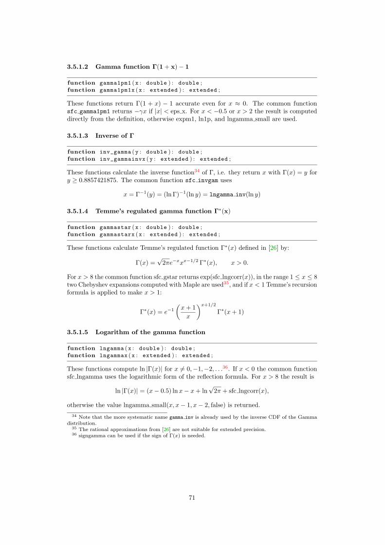
3.5.1.2 Gamma function Γ(1 + x)− 1

function gamma1pm1 (x : double ) : double ;function gamma1pm1x (x : extended ) : extended ;

These functions return Γ(1 + x) − 1 accurate even for x ≈ 0. The common functionsfc gamma1pm1 returns −γx if |x| < eps x. For x < −0.5 or x > 2 the result is computeddirectly from the definition, otherwise expm1, ln1p, and lngamma small are used.

3.5.1.3 Inverse of Γ

function inv_gamma (y : double ) : double ;function inv_gammainvx (y : extended ) : extended ;

These functions calculate the inverse function34 of Γ, i.e. they return x with Γ(x) = y fory ≥ 0.8857421875. The common function sfc invgam uses

x = Γ−1(y) = (ln Γ)−1(ln y) = lngamma inv(ln y)

3.5.1.4 Temme’s regulated gamma function Γ∗(x)

function gammastar (x : double ) : double ;function gammastarx (x : extended ) : extended ;

These functions calculate Temme’s regulated function Γ∗(x) defined in [26] by:

Γ(x) =√

2πe−xxx−1/2 Γ∗(x), x > 0.

For x > 8 the common function sfc gstar returns exp(sfc lngcorr(x)), in the range 1 ≤ x ≤ 8two Chebyshev expansions computed with Maple are used35, and if x < 1 Temme’s recursionformula is applied to make x > 1:

Γ∗(x) = e−1

(x+ 1x

)x+1/2

Γ∗(x+ 1)

3.5.1.5 Logarithm of the gamma function

function lngamma (x : double ) : double ;function lngammax (x : extended ) : extended ;

These functions compute ln |Γ(x)| for x 6= 0,−1,−2, . . .36. If x < 0 the common functionsfc lngamma uses the logarithmic form of the reflection formula. For x > 8 the result is

ln |Γ(x)| = (x− 0.5) lnx− x+ ln√

2π + sfc lngcorr(x),

otherwise the value lngamma small(x, x− 1, x− 2, false) is returned.

34 Note that the more systematic name gamma inv is already used by the inverse CDF of the Gammadistribution.

35 The rational approximations from [26] are not suitable for extended precision.36 signgamma can be used if the sign of Γ(x) is needed.

71

3.5.1.6 Inverse of lnΓ

function lngamma_inv (y : double ) : double ;function lngamma_invx (y : extended ) : extended ;

These functions calculate the inverse function of ln Γ, i.e. they return x = lngamma inv(y)with ln Γ(x) = y for y ≥ −0.12142 > ym (the minimum of ln Γ(x) for positive arguments),the result is greater than xm = 1.46163 . . . (the positive zero of the ψ function). Thecommon function sfc ilng computes the zero x > xm of the function f(x) = ln Γ(y)− xusing Newton’s method

xn+1 = xn −f(xn)f ′(xn)

= xn −ln Γ(xn)− y

ψ(xn),

where the starting values x0 are taken from four different cases.37

3.5.1.7 Logarithm of Γ(1 + x)

function lngamma1p (x : double ) : double ;function lngamma1px (x : extended ) : extended ;

These functions compute ln |Γ(1 + x)| with increased accuracy for x ≈ 0. For x < −1 orx > 7 the result is calculated as lngamma(1 + x) otherwise the value lngamma small(x+1, x, x− 1, true) is returned.

3.5.1.8 Reciprocal gamma function

function rgamma (x : double ) : double ;function rgammax (x : extended ) : extended ;

These routines calculate the reciprocal gamma function 1/Γ(x), which is an entire functionwith simple zeros at the points x = 0 and the negative integers. If |x| < 0.03125 thecommon function sfc rgamma returns sfc gaminv small(x), for x ∈ [−0.5, 8] the result iscomputed with the sfc gamma medium function just from the definition, and otherwise

1/Γ(x) = sign(Γ(x)

)exp

(− ln |Γ(x)|

).

3.5.1.9 Sign of gamma function

function signgamma (x : double ) : double ;function signgammax (x : extended ) : extended ;

These functions return the sign of Γ(x), which is +1 if x > 0 or if bxc is even, −1otherwise38.

3.5.1.10 Logarithm and sign of gamma function

function lngammas (x : double ; var s : integer ) : double ;function lngammasx (x : extended ; var s : integer ) : extended ;

These functions return ln |Γ(x)| using lngamma(x) and s is the sign of Γ(x).

37 E.g. for y ≥ 10 from a simplified inverted Stirling approximation.38 The sign is meaningless for x = 0 or negative integers.

72

3.5.2 Incomplete gamma functions

The incomplete gamma functions are defined as

γ(a, x) =∫ x

0

ta−1e−t dt a 6= 0,−1,−2, . . . ,

Γ(a, x) =∫ ∞

x

ta−1e−t dt,

or in their normalised forms

P (a, x) =γ(a, x)Γ(a)

Q(a, x) =Γ(a, x)Γ(a)

An important internal routine for the incomplete gamma code is:

function sfc_igprefix (a , x : extended ) : extended ;

This function returns e−xxa/Γ(a), which is the most sensible single term controlling therounding errors occurring in computation of the incomplete gamma functions, see [26,3.3]. It is implemented with the Lanczos sum from Boost[19] file gamma.hpp, functionregularised gamma prefix.

3.5.2.1 Normalised incomplete gamma functions

procedure incgamma (a , x : double ; var p , q : double ) ;procedure incgammax (a , x : extended ; var p , q : extended ) ;

These procedures simultaneously compute the normalised incomplete gamma functions

P (a, x) =1

Γ(a)

∫ x

0

ta−1e−t dt, Q(a, x) =1

Γ(a)

∫ ∞

x

ta−1e−t dt

for a ≥ 0 and x ≥ 0. The implementation of the common function sfc incgamma39 isheavily based on Temme’s paper and algorithms [26], except in the asymptotic case a ∼ xfor large a, where the algorithm from Boost[19] igamma large.hpp is used.40

function igammap (a , x : double ) : double ;function igammapx (a , x : extended ) : extended ;

These functions return the normalised lower incomplete gamma function P (a, x)

P (a, x) =1

Γ(a)

∫ x

0

ta−1e−t dt

for a ≥ 0 and x ≥ 0 using a call to sfc incgamma. If a = x = 0 then P = 0.5, otherwiseP = 0 if x = 0 and P = 1 if a = 0.

function igammaq (a , x : double ) : double ;function igammaqx (a , x : extended ) : extended ;

These functions return the normalised upper incomplete gamma function Q(a, x)

Q(a, x) =1

Γ(a)

∫ ∞

x

ta−1e−t dt

for a ≥ 0 and x ≥ 0 using a call to sfc incgamma. If a = x = 0 then Q = 0.5, otherwiseQ = 1 if x = 0 and Q = 0 if a = 0.

39 Actually in sfc incgamma ex where the prefix calculation is optional.40 Temme’s pqasymp with it’s ≈ 10 digit accuracy is not suitable for extended precision.

73

3.5.2.2 Non-normalised incomplete gamma functions

function igamma (a , x : double ) : double ;function igammax (a , x : extended ) : extended ;

These functions return the non-normalised upper incomplete gamma function

Γ(a, x) =∫ ∞

x

ta−1e−t dt

for x ≥ 0. Special cases are Γ(a, 0) = Γ(a) and Γ(0, x) = E1(x).If a < 0, the parameter ranges for the calculation are as follows: For x > 1/4 or

a ≤ −10000 the Legendre continued fraction from Abramowitz/Stegun [1, 6.5.31]

Γ(a, x) = e−xxa

(1x+

1− a

1+1x+

2− a

1+2x+

· · ·)

(3.5)

is computed using the Temme/Gautschi form [26, procedure qfraction]. If a ≥ −1/2 theTaylor expansion for Q(a, x) is used, and otherwise the recurrence relation from Olver etal. [30, 8.8.2]: Γ(a+ 1, x) = aΓ(a, x) + xae−x.

For a > 0 the result is just Γ(a, x) = Q(a, x)Γ(a), if Γ(a) will not overflow. For larger avalues the continued fraction is used if e−xxa will not overflow, otherwise the logarithmicform lnΓ(a, x) = lnQ(a, x) + lnΓ(a) is applied.

function igammal (a , x : double ) : double ;function igammalx (a , x : extended ) : extended ;

These functions return the non-normalised lower incomplete gamma function γ(a, x) forx ≥ 0 and a 6= 0,−1,−2, . . .

γ(a, x) =∫ x

0

ta−1e−t dt

The result is γ(a, x) = Γ(a)− Γ(a, x) or γ(a, x) = P (a, x)Γ(a) (or it’s logarithmic form)except if x < a− 1/4 or x < 4 and Γ(a) overflows: In this case the Taylor expansion forP (a, x) from [26, (5.5)] is used. At the zeros of γ(a, x) for a < 0 only absolute accuracy isachievable, if it is less than half of the precision debug mode warnings are available.

3.5.2.3 Tricomi’s entire incomplete gamma function

function igammat (a , x : double ) : double ;function igammatx (a , x : extended ) : extended ;

These functions return Tricomi’s entire incomplete gamma function γ∗, defined for a > 0by the integral [30, 8.2.7]

γ∗(a, x) =1

Γ(a)

∫ 1

0

ta−1e−tx dt, a > 0,

and by analytic continuation with Kummer’s confluent hypergeometric M function as anentire function of both arguments for all a, x

γ∗(a, x) = e−x M(1, a+ 1, x)Γ(a+ 1)

= e−x∞∑

n=0

xn

Γ(a+ n+ 1).

Special cases are γ∗(0, x) = 1, γ∗(a, 0) = 1/Γ(a + 1), and γ∗(−n, x) = xn, if −n is anegative integer. Otherwise there are the following relations to other incomplete gammafunctions (see Olver et. al [30, 8.2.6]):

γ∗(a, x) =x−a

Γ(a)γ(a, x) = x−aP (a, x).

74

The common function sfc git handles the special cases, and uses the full hypergeometricfunction sfc 1f1 if x < 0.

Some of the hard cases for x > 0 (where separate Γ(a) terms would over/underflow) arehandled with code snippets from SLATEC [14, 20, files dgamit.f, d9lgic.f]. When a > x+ 1or a < 0, x < 1 the result is computed with a simple Kummer series, and if a < 0, x ≥ 1the function is evaluated as

γ∗(a, x) =Γ(a)− Γ(a, x)

Γ(a)x−a.

At the non-trivial zeros of γ∗ (e.g. if the above numerator vanishes, similar for the otherparameter cases) only absolute accuracy is achievable; if it is less than half of the extendedprecision, sfc git can emit debug mode warnings.

3.5.2.4 Inverse normalised incomplete gamma functions

This section describes the procedures and functions for the functional inverses of thenormalised incomplete gamma functions; in AMath they are used for inverting thegamma and chi-square distributions. The classical reference is the article and FORTRANcode by A.R. DiDonato and A.H. Morris [27].

procedure incgamma_inv (a , p , q : double ; var x : double ;var ierr : integer ) ;

procedure incgamma_invx (a , p , q : extended ; var x : extended ;var ierr : integer ) ;

These procedures return the inverse normalised incomplete gamma function, i.e. theycalculate x with P (a, x) = p and Q(a, x) = q. The input parameters are a > 0, p ≥ 0,q ≥ 0, and p + q = 1. The output parameter ierr is ≥ 0 for success, and < 0 for inputerrors or iterations failures:

≥ 0 iteration count= -2 if a ≤ 0= -4 if p < 0, q < 0, or |p+ q − 1| > eps d= -6 if 10 iterations were performed= -7 iteration failed= -8 x is calculated with unknown accuracy

The common procedure sfc incgamma inv is divided into three parts: In the first partthe input parameters are checked; note that the condition p + q = 1 is evaluated as|p+ q−1| ≤ eps d because the parameters may be casts from double precision. The second(main) part is the sophisticated guessing of the initial value for x, and finally this value isimproved by Schroder or Newton iteration steps; note that the iteration count may bezero if the initial guess is good enough. In the AMath Pascal source code the originaltext and equations from DiDonato and Morris [27] are used for easy reference41.

function igamma_inv (a , p , q : double ) : double ;function igamma_invx (a , p , q : extended ) : extended ;

These functions return the inverse normalised incomplete gamma function, i.e. theycalculate x with P (a, x) = p and Q(a, x) = q. The input parameters are a > 0, p ≥ 0,q ≥ 0, and p+ q = 1. The routines finally use sfc incgamma inv and raise error conditionsinstead of returning negative error codes.

41 Together with the Boost[19] interpretation from igamma inverse.hpp

75

function igammap_inv (a , p : double ) : double ;function igammap_invx (a , p : extended ) : extended ;

These functions return the inverse normalised lower incomplete gamma function, i.e. theycalculate x with P (a, x) = p with a > 0, 0 ≤ p < 1 using sfc incgamma inv and raiseerror conditions instead of returning negative error codes.

function igammaq_inv (a , q : double ) : double ;function igammaq_invx (a , q : extended ) : extended ;

These functions return the inverse normalised upper incomplete gamma function, i.e. theycalculate x with Q(a, x) = q with a > 0, 0 < q ≤ 1, using sfc incgamma inv and raiseerror conditions instead of returning negative error codes.

3.5.3 Beta functions

An important internal routine for the incomplete beta function and related code is:

function sfc_ibetaprefix (a , b , x , y : extended ) : extended ;

This function returns xayb/B(a, b) using Lanczos approximation from the Boost[19] filebeta.hpp, function ibeta power terms.

3.5.3.1 Beta function B(x,y)

function beta (x , y : double ) : double ;function betax (x , y : extended ) : extended ;

These functions calculate the beta function, which is defined as

B(x, y) =Γ(x)Γ(y)Γ(x+ y)

·

If one argument is 1, the inverse of the other is returned. If both x, y > 0 then the commonfunction sfc beta uses the Lanczos expression from Boost [19, beta.hpp], otherwise whenx ≤ 0 or y ≤ 0 and x+ y is not an non-positive integer the result is computed as42

B(x, y) = signB(x, y) exp(lnbeta(x, y)).

Special considerations are needed if x + y actually is a non-positive integer: If x andy are no integers then B = 0. Since B(x, y) is symmetric, let x ≤ y. If y > 0 thenB(x, y) = Γ(y)/(x)y, otherwise the result is undefined.

3.5.3.2 Logarithm of the beta function

function lnbeta (x , y : double ) : double ;function lnbetax (x , y : extended ) : extended ;

These functions compute the logarithm of the beta function ln |B(x, y)| with x, y 6=0,−1,−2, . . . Since the function is symmetric, let x ≤ y. The implementation is based onthe SLATEC [14] routine dlbeta.f. Let s = x+ y. If x ≥ 8 then

ln |B(x, y)| = −0.5 ln y + ln√

2π + c1 + (x− 0.5) ln(x/s) + yln1p(−x/s)42 sign B(x, y) = sign Γ(x) signΓ(y)/ sign Γ(x + y)

76

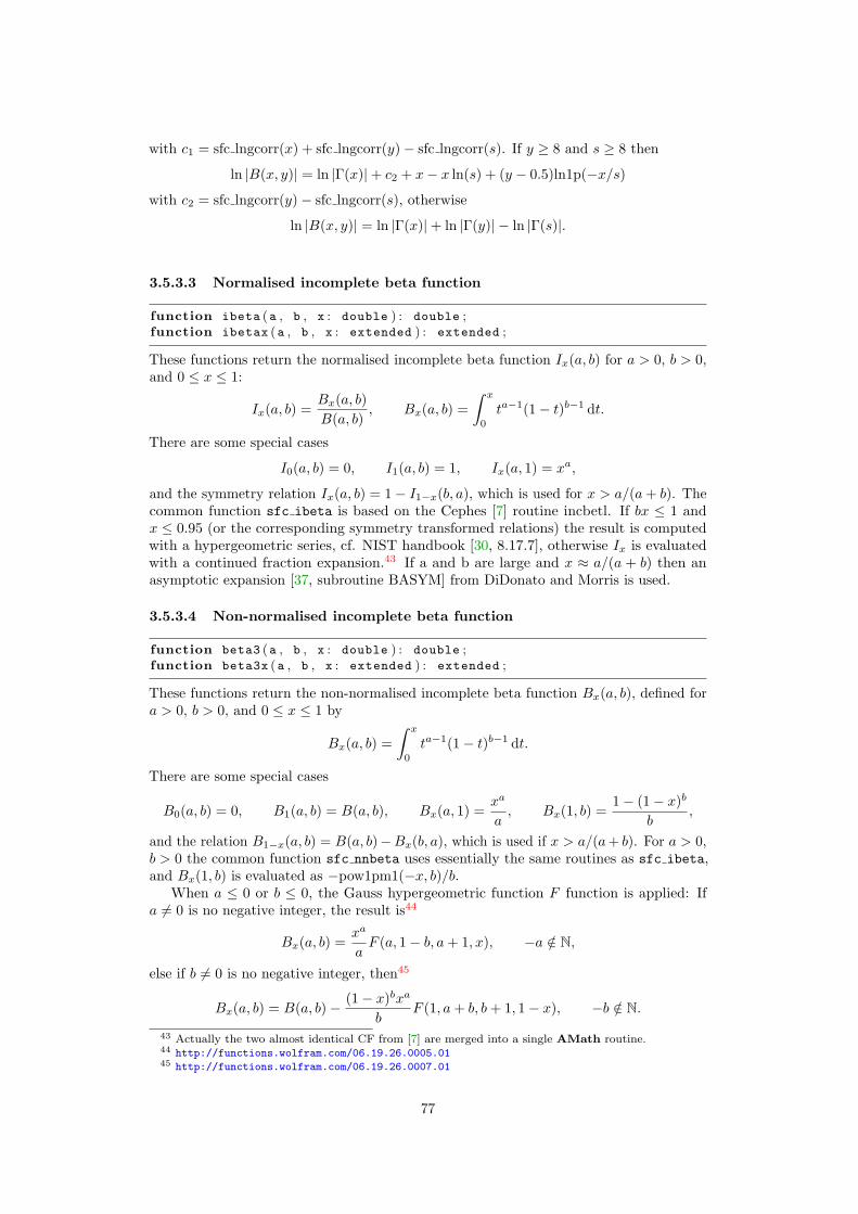
with c1 = sfc lngcorr(x) + sfc lngcorr(y)− sfc lngcorr(s). If y ≥ 8 and s ≥ 8 then

ln |B(x, y)| = ln |Γ(x)|+ c2 + x− x ln(s) + (y − 0.5)ln1p(−x/s)

with c2 = sfc lngcorr(y)− sfc lngcorr(s), otherwise

ln |B(x, y)| = ln |Γ(x)|+ ln |Γ(y)| − ln |Γ(s)|.

3.5.3.3 Normalised incomplete beta function

function ibeta (a , b , x : double ) : double ;function ibetax (a , b , x : extended ) : extended ;

These functions return the normalised incomplete beta function Ix(a, b) for a > 0, b > 0,and 0 ≤ x ≤ 1:

Ix(a, b) =Bx(a, b)B(a, b)

, Bx(a, b) =∫ x

0

ta−1(1− t)b−1 dt.

There are some special cases

I0(a, b) = 0, I1(a, b) = 1, Ix(a, 1) = xa,

and the symmetry relation Ix(a, b) = 1− I1−x(b, a), which is used for x > a/(a+ b). Thecommon function sfc ibeta is based on the Cephes [7] routine incbetl. If bx ≤ 1 andx ≤ 0.95 (or the corresponding symmetry transformed relations) the result is computedwith a hypergeometric series, cf. NIST handbook [30, 8.17.7], otherwise Ix is evaluatedwith a continued fraction expansion.43 If a and b are large and x ≈ a/(a + b) then anasymptotic expansion [37, subroutine BASYM] from DiDonato and Morris is used.

3.5.3.4 Non-normalised incomplete beta function

function beta3 (a , b , x : double ) : double ;function beta3x (a , b , x : extended ) : extended ;

These functions return the non-normalised incomplete beta function Bx(a, b), defined fora > 0, b > 0, and 0 ≤ x ≤ 1 by

Bx(a, b) =∫ x

0

ta−1(1− t)b−1 dt.

There are some special cases

B0(a, b) = 0, B1(a, b) = B(a, b), Bx(a, 1) =xa

a, Bx(1, b) =

1− (1− x)b

b,

and the relation B1−x(a, b) = B(a, b)−Bx(b, a), which is used if x > a/(a+ b). For a > 0,b > 0 the common function sfc nnbeta uses essentially the same routines as sfc ibeta,and Bx(1, b) is evaluated as −pow1pm1(−x, b)/b.

When a ≤ 0 or b ≤ 0, the Gauss hypergeometric function F function is applied: Ifa 6= 0 is no negative integer, the result is44

Bx(a, b) =xa

aF (a, 1− b, a+ 1, x), −a /∈ N,

else if b 6= 0 is no negative integer, then45

Bx(a, b) = B(a, b)− (1− x)bxa

bF (1, a+ b, b+ 1, 1− x), −b /∈ N.

43 Actually the two almost identical CF from [7] are merged into a single AMath routine.44 http://functions.wolfram.com/06.19.26.0005.0145 http://functions.wolfram.com/06.19.26.0007.01

77

3.5.3.5 Inverse normalised incomplete beta function

function ibeta_inv (a , b , y : double ) : double ;function ibeta_invx (a , b , y : extended ) : extended ;

These functions calculate the inverse of normalised incomplete beta function for a, b > 0and 0 ≤ y ≤ 1, i.e. they return x = ibeta inv(a, b, y) with Ix(a, b) = y. The commonfunction sfc ibeta inv is based on Cephes [7, ldouble/incbil.c], the result is computedwith Newton iterations or bisections using the starting value

√2 erfc−1(2y).

3.5.4 Factorials, Pochhammer symbol, binomial coefficient

3.5.4.1 Factorial

function fac (n : integer ) : double ;function facx (n : integer ) : extended ;

These functions return the factorial n! = n× (n− 1)× · · · × 2× 1. If n < 0 the result is∞, for n < 25 the value is taken from a table, and otherwise n! = Γ(n+ 1) is computedwith the stirf function.

3.5.4.2 Double factorial

function dfac (n : integer ) : double ;function dfacx (n : integer ) : extended ;

These functions return the double factorial n!!, for even n < 0 the result is ∞. For positiven the double factorial is defined as

n!! =

{1 · 3 · 5 · · ·n if n is odd,2 · 4 · 6 · · ·n if n is even.

The common function sfc dfac computes the result depending on one of the followingcases46 with integer k ≥ 0:

(2k)!! = 2kk!

(2k + 1)!! = (2k + 1)!/(2kk!) =2k+1

√π

Γ(k + 3

2

)(−2k − 1)!! = (−1)k/(2k − 1)!!

3.5.4.3 Logarithm of factorials

function lnfac (n : longint ) : double ;function lnfacx (n : longint ) : extended ;

These functions return ln(n!). If n < 0 the result is ∞, for n < 25 it is computed from atable, otherwise ln(n!) = sfc lngamma(n+ 1).

46 Γ is called explicitly for odd n > 25.

78

3.5.4.4 Binomial coefficient

function binomial (n , k : integer ) : double ;function binomialx (n , k : integer ) : extended ;

These functions return the binomial coefficient (”n choose k”) defined as(n

k

)=n(n− 1) · · · (n− k + 1)

k(k − 1) · · · (1)

for k ≥ 0. If n < 0 or k < 0 there are two non-trivial ranges: For n < 0 and k ≥ 0 thecoefficients are calculated with Knuth’s [32] identity 1.2.6 (17)(

n

k

)= (−1)k

(k − n− 1

k

)and for k ≤ n < 0 with [32, 1.2.6 (19)](

n

k

)= (−1)n−k

(−k − 1n− k

).

In the common function sfc binomial these cases are handled with recursive calls. In the’normal’ range 0 ≤ k ≤ n the result is calculated as n!/(n− k)!/k! if n < 1755, i.e. n! doesnot overflow. If k ≤ 400047 and a rough estimate shows that there will be no overflow thevalue is computed as a product of quotients as in the definition. Otherwise the lnbetafunction is used to return(

n

k

)=(k exp(lnbeta(k, n− k + 1))

)−1

.

The unusual complicated form is chosen to minimize overflow risk while maintainingreasonable accuracy. The table shows the RMS and peak relative errors calculated forrandom input samples:

Range (n) Samples RMS Peak (n,k)0.. 1000 20000 1.2087E-19 5.9631E-19 for (820,415)

1000.. 1700 20000 1.4733E-19 6.5052E-19 for (1678,331)1700.. 8000 20000 1.4177E-18 7.4801E-18 for (7185,4779)8000..16000 10000 2.0377E-16 1.2166E-15 for (14557,6857)

16000..32000 10000 1.8608E-16 1.2806E-15 for (18717,4636)

3.5.4.5 Pochhammer symbol

function pochhammer (a , x : double ) : double ;function pochhammerx (a , x : extended ) : extended ;

These functions return the Pochhammer symbol (a)x = Γ(a+ x)/Γ(a). In the special casethat x = n is a positive integer, (a)n = a(a+ 1)(a+ 2) · · · (a+n− 1) is often called ”risingfactorial”. By convention (a)0 = 1.

If a or a+ x are negative integers or zero special care must be taken: If only a is aninteger then the result is zero. If a+ x is also a negative integer the Pochhammer symbolis computed from the limiting form of the Γ reflection formula

(a)x = (−1)x Γ(1− a)Γ(1− a− x)

,

and otherwise the function is undefined. If a and a + x are no negative integers, (a)x

is calculated from the definition.The common function sfc pochhammer computes bothgamma function ratios with the gamma delta ratio function.

47 k is replaced by n− k if it is > n/2.

79

3.5.4.6 Relative Pochhammer symbol

function poch1 (a , x : double ) : double ;function poch1x (a , x : extended ) : extended ;

These functions compute the relative Pochhammer symbol defined as

poch1(a, x) =(a)x − 1

x,

accurate even for small x. The common function sfc poch1 is a translation of the routinedpoch1.f by Fullerton [14, 20].

If |x| is small, cancellation errors are avoided by using an expansion by Fields and Lukewith generalized Bernoulli polynomials. For x = 0 the value ψ(a) is returned, otherwisethe result is calculated from the definition.

3.5.5 Ratio of gamma functions

function gamma_delta_ratio (x , d : double ) : double ;function gamma_delta_ratiox (x , d : extended ) : extended ;

These functions compute Γ(x)/Γ(x+d), accurate even for |d| � |x|. If x > 0 and x+d > 0the Pascal code uses Lanczos sums and is based on the corresponding Boost [19] functionin gamma.hpp, the case x < 0 and x+ d < 0 is reduced to the former with a reflectionformula. If x and x+ d have different signs, the result is computed with calls to lngamma.

function gamma_ratio (x , y : double ) : double ;function gamma_ratiox (x , y : extended ) : extended ;

These routines return the gamma function ratio Γ(x)/Γ(y). The common function simplycalls gamma delta ratio(x, y − x).

3.5.6 Psi and polygamma functions

3.5.6.1 Digamma function ψ(x)

function psi (x : double ) : double ;function psix (x : extended ) : extended ;

These functions return the digamma or ψ function, which is defined as

ψ(x) = d(ln Γ(x))/dx = Γ′(x)/Γ(x), x 6= 0,−1,−2, . . .

For x > 12 the common function sfc psi evaluates digamma with the asymptotic expan-sion from Abramowitz and Stegun [1, 6.3.18]

ψ(x) ∼ lnx− 12x−

∞∑n=1

B2n

2nx2n

If x < 0 it is transformed to positive values with the reflection formula [1, 6.3.7]

ψ(1− x) = ψ(x) + π cotπx,

80

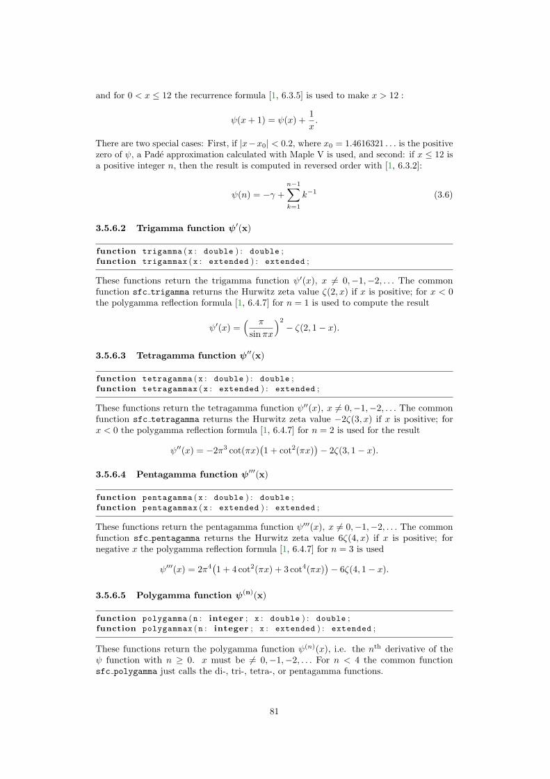
and for 0 < x ≤ 12 the recurrence formula [1, 6.3.5] is used to make x > 12 :

ψ(x+ 1) = ψ(x) +1x.

There are two special cases: First, if |x−x0| < 0.2, where x0 = 1.4616321 . . . is the positivezero of ψ, a Pade approximation calculated with Maple V is used, and second: if x ≤ 12 isa positive integer n, then the result is computed in reversed order with [1, 6.3.2]:

ψ(n) = −γ +n−1∑k=1

k−1 (3.6)

3.5.6.2 Trigamma function ψ′(x)

function trigamma (x : double ) : double ;function trigammax (x : extended ) : extended ;

These functions return the trigamma function ψ′(x), x 6= 0,−1,−2, . . . The commonfunction sfc trigamma returns the Hurwitz zeta value ζ(2, x) if x is positive; for x < 0the polygamma reflection formula [1, 6.4.7] for n = 1 is used to compute the result

ψ′(x) =( π

sinπx

)2

− ζ(2, 1− x).

3.5.6.3 Tetragamma function ψ′′(x)

function tetragamma (x : double ) : double ;function tetragammax (x : extended ) : extended ;

These functions return the tetragamma function ψ′′(x), x 6= 0,−1,−2, . . . The commonfunction sfc tetragamma returns the Hurwitz zeta value −2ζ(3, x) if x is positive; forx < 0 the polygamma reflection formula [1, 6.4.7] for n = 2 is used for the result

ψ′′(x) = −2π3 cot(πx)(1 + cot2(πx)

)− 2ζ(3, 1− x).

3.5.6.4 Pentagamma function ψ′′′(x)

function pentagamma (x : double ) : double ;function pentagammax (x : extended ) : extended ;

These functions return the pentagamma function ψ′′′(x), x 6= 0,−1,−2, . . . The commonfunction sfc pentagamma returns the Hurwitz zeta value 6ζ(4, x) if x is positive; fornegative x the polygamma reflection formula [1, 6.4.7] for n = 3 is used

ψ′′′(x) = 2π4(1 + 4 cot2(πx) + 3 cot4(πx)

)− 6ζ(4, 1− x).

3.5.6.5 Polygamma function ψ(n)(x)

function polygamma (n : integer ; x : double ) : double ;function polygammax (n : integer ; x : extended ) : extended ;

These functions return the polygamma function ψ(n)(x), i.e. the nth derivative of theψ function with n ≥ 0. x must be 6= 0,−1,−2, . . . For n < 4 the common functionsfc polygamma just calls the di-, tri-, tetra-, or pentagamma functions.

81

For x > 0 the result is calculated with the series expansion [1, 6.4.10]

ψ(n)(x) = (−1)n+1n!∞∑

k=0

(x+ k)−n−1 = (−1)n+1n! ζ(n+ 1, x). (3.7)

If the actual computed extended value ζ(n+ 1, x) of the Hurwitz zeta function is zero,the asymptotic formula [1, 6.4.11] is used:

ψ(n)(x) ∼ (−1)n−1

((n− 1)!xn

+n!

2xn+1+

∞∑k=1

B2k(2k + n− 1)!(2k)!x2k+n

)

In extreme parameter cases a term in the asymptotic formula can cause overflow(e.g. for polygamma(5000, 200) ≈ −0.149687668E4819) or there is no convergence withinreasonable limits (e.g. for polygamma(4000, 200) ≈ −0.69367177835736E3467); in thesesituations the series expansion (3.7) is evaluated in the form

ψ(n)(x) = (−1)n+1 Γ(n+ 1)xn+1

∞∑k=0

1(1 + k/x)n+1

.

For x < 0 the polygamma reflection formula [1, 6.4.7] is used

ψ(n)(1− x) + (−1)n+1ψ(n)(x) = (−1)nπdn

dxncot(πx) (3.8)

with pre-computed coefficients of the polynomials pn(cot(πx)) from the nth derivative ofcot(πx) if n ≤ 12 and for n ≥ 70 with a series for the RHS of 3.8

(−1)n

(1x

+∞∑

k=1

(1

x+ k+

1x− k

))(n)

= n!

(1

xn+1+

∞∑k=1

(1

(x+ k)n+1+

1(x− k)n+1

))

derived from Euler’s series for π cot(πx). For 12 < n < 70 the polynomials are used withdynamically computed coefficients, if the presumed convergence of the series is slow.

3.5.6.6 Inverse digamma function ψ−1(y)

function psi_inv (y : double ) : double ;function psi_invx (y : extended ) : extended ;

These routines return the functional inverse ψ−1(y) of the digamma function ψ fory ≤ ln(MaxExtended). The common function sfc ipsi computes the result x usingNewton’s root finding method for f(x) = ψ(x)− y with the trigamma function ψ′

xn+1 = xn −f(xn)f ′(xn)

= xn −ψ(xn)− y

ψ′(xn)·

The starting values x0 are taken from three different cases.

82

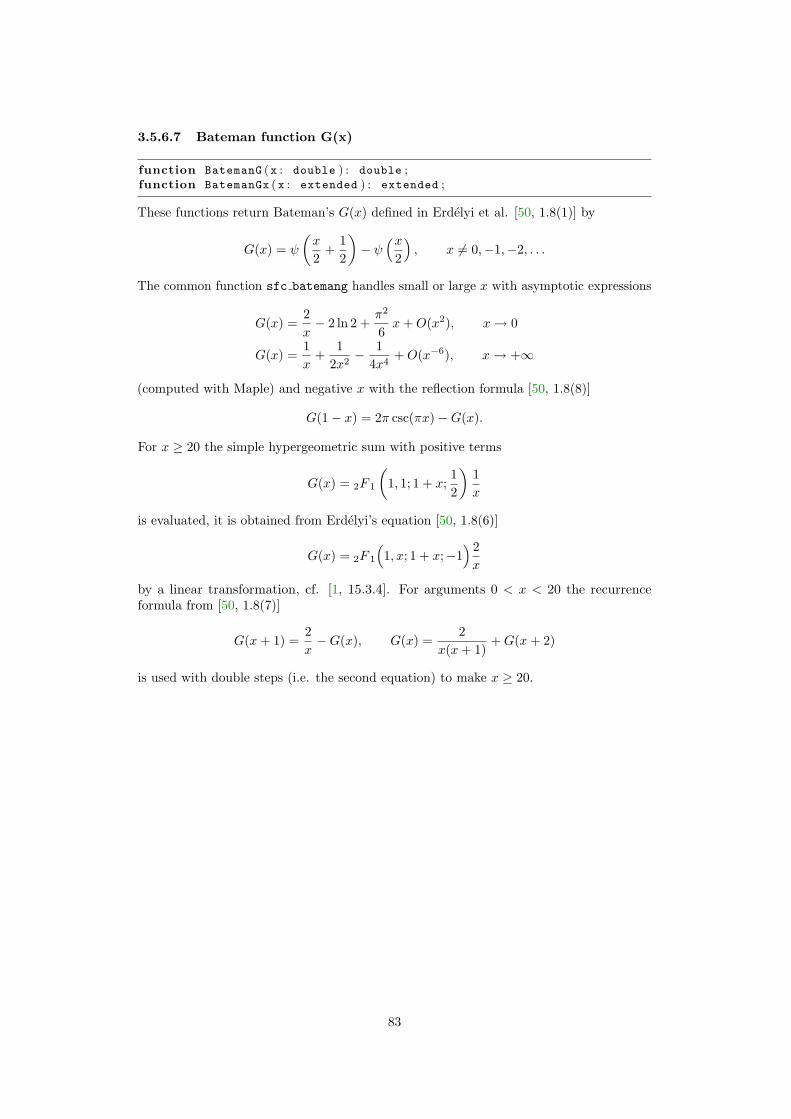
3.5.6.7 Bateman function G(x)

function BatemanG (x : double ) : double ;function BatemanGx (x : extended ) : extended ;

These functions return Bateman’s G(x) defined in Erdelyi et al. [50, 1.8(1)] by

G(x) = ψ

(x

2+

12

)− ψ

(x2

), x 6= 0,−1,−2, . . .

The common function sfc batemang handles small or large x with asymptotic expressions

G(x) =2x− 2 ln 2 +

π2

6x+O(x2), x→ 0

G(x) =1x

+1

2x2− 1

4x4+O(x−6), x→ +∞

(computed with Maple) and negative x with the reflection formula [50, 1.8(8)]

G(1− x) = 2π csc(πx)−G(x).

For x ≥ 20 the simple hypergeometric sum with positive terms

G(x) = 2F 1

(1, 1; 1 + x;

12

)1x

is evaluated, it is obtained from Erdelyi’s equation [50, 1.8(6)]

G(x) = 2F 1

(1, x; 1 + x;−1

) 2x

by a linear transformation, cf. [1, 15.3.4]. For arguments 0 < x < 20 the recurrenceformula from [50, 1.8(7)]

G(x+ 1) =2x−G(x), G(x) =

2x(x+ 1)

+G(x+ 2)

is used with double steps (i.e. the second equation) to make x ≥ 20.

83

3.6 Zeta functions, polylogarithms, and related

The unit sfZeta implements the common code for the zeta functions, polylogarithms, andrelated functions.

There are two important basic internal functions, which are called by the other commonroutines in the η/ζ function group. In this section let ηε = 10−9, for |s| ≤ ηε the etafunctions are linear (accurate to extended precision).

function etam1pos (s : extended ) : extended ;

This function returns the Dirichlet η(s)− 1 function for s ≥ −ηε

η(s)− 1 = −∞∑

k=2

(−1)k

ks·

If |s| ≤ ηε the result is (s ln(π/2)−1)/2. Otherwise the powers ks are computed with primepowers, but only if necessary. If s < 19.5 the powers up to k24 are used with P. Borwein’s[36] convergence acceleration technique.48

function zetap (s , sc : extended ) : extended ;

This function returns the Riemann zeta function for s > 0, s 6= 1. The parameter sc = 1−sis externally supplied to increase the accuracy. The routine is based on Boost’s [19]zeta.hpp and uses six rational approximations in the range 0 < s < 42.

3.6.1 Riemann zeta functions

3.6.1.1 Riemann ζ(s) function

function zeta (s : double ) : double ;function zetax (s : extended ) : extended ;

These functions calculate the Riemann zeta function ζ(s) for s 6= 1, defined by

ζ(s) =∞∑

k=1

1ks, s > 1,

and by analytic continuation for s 6= 1. When s = 0 the result is −1/2, and for s > 0the common function sfc zeta returns zetap(s, 1− s). If s < 0 the reflection formula [30,25.4.2] is used:

ζ(s) = 2(2π)s−1 sin( 12πs)Γ(1− s)ζ(1− s)

3.6.1.2 Riemann ζ(n) for integer arguments

function zetaint (n : integer ) : double ;function zetaintx (n : integer ) : extended ;

These functions return the Riemann zeta function ζ(n) for integer arguments n 6= 1. Forn > 63 the result is 1, for 0 ≤ n ≤ 63 the value is taken from table, otherwise the Bernoullinumbers are used: ζ(n) = B1−n/(n− 1) for n < 0.

48 The coefficients are from Algorithm 2, but re-calculated, scaled, and shifted with Maple; DAMathuses powers up to k21 for s < 17.

84

3.6.1.3 Riemann ζ(1 + x)

function zeta1p (x : double ) : double ;function zeta1px (x : extended ) : extended ;

These functions calculate the Riemann zeta function ζ(1 + x) for x 6= 0. Normally usedwith |x| � 1 for increased accuracy near the pole of ζ(s) at s = 1. The common functionsfc zeta1p returns zetap(1 + x,−x) for |x| < 1, and ζ(1 + x) otherwise.

3.6.1.4 Riemann ζ(s)− 1

function zetam1 (s : double ) : double ;function zetam1x (s : extended ) : extended ;

These functions evaluate the Riemann function ζ(s)− 1 for s 6= 1. They are provided asseparate routines because ζ(s) → 1 for large s, in fact ζ(s) = 1 to extended precision fors ≥ 64. The common function sfc zetam1 returns ζ(s)− 1 for s ≤ 2, and 2−s if s ≥ 120,otherwise the result is computed as

ζ(s)− 1 =1 + (η(s)− 1)2s−1

2s−1 − 1·

3.6.2 Prime zeta function

function primezeta (x : double ) : double ;function primezetax (x : extended ) : extended ;

These functions return the prime zeta function (or its real part for x < 1)

P (x) =∑

p prime

p−x, x > 15 ·

In the implemented range P has singularities at 1/3, 1/2, 1 and the imaginary part=P (x) is π

6 for 15 < x < 1

3 ,π2 for 1

3 < x < 12 , and π for 1

2 < x < 1.49

For x ≥ 27 the common function sfc pz uses the first significant terms of the sum upto 7−x, otherwise the calculation is based on

P (x) =∞∑

n=1

µ(n)n

ln(ζ(nx)),

where µ is the Mobius function50. Actually P (x) is computed with Cohen’s speed-up51

P (x) =∑p≤A

p−x +∑n≥1

µ(n)n

ln(ζp>A(nx))

ζp>A(s) = ζ(s)∏p≤A

(1− p−s)

Since ζ(nx) rapidly approaches 1, the sum is evaluated with the accuracy improvedfunctions ln1p and zetam1 (if nx > 1) in order to minimise rounding and truncation errors.

49 P (x) has an infinite number of singularities at x = 1n

where n is a square-free integer (i.e. nx = 1and µ(n) 6= 0); this is a reason why P (x) cannot be continued to x ≤ 0, and computationally an increasingnumber of terms in the series is needed (AMath uses up to 95 for x ≈ 1

5).

50 µ(n) = 1 if n = 1 or n is a product of an even number of distinct primes, µ(n) = −1 if n is a productof an odd number of distinct primes, and µ(n) = 0 if n has a multiple prime factor.

51 See e.g. http://www.math.u-bordeaux.fr/~cohen/hardylw.dvi, section 2.1; AMath implementsthe speed-up with A = 7.

85

3.6.3 Dirichlet eta functions

3.6.3.1 Dirichlet eta function

function eta (s : double ) : double ;function etax (s : extended ) : extended ;

These functions return the Dirichlet function η(s), also known as the alternating zetafunction, defined for s > 0 as

η(s) =∞∑

n=1

(−1)n−1

ns

and by analytic continuation for s ≤ 0. The important relation to the Riemann zetafunction is η(s) = (1 − 21−s)ζ(s), which is directly evaluated for s ≤ −8. In the range−8 < s < −ηε the reflection formula52 for η is used:

η(s) =2(1− 21−s)Γ(1− s) cos( 1

2π(1− s))(1− 2s)(2π)1−s

η(1− s)

and for s ≥ −ηε the common function sfc eta returns 1 + etam1pos(s).

3.6.3.2 Dirichlet eta function for integer arguments

function etaint (n : integer ) : double ;function etaintx (n : integer ) : extended ;

These functions return the Dirichlet eta function η(n) for integer arguments. For n > 64the result is 1, for 0 ≤ n ≤ 64 the value is taken from table, otherwise for n < 0 theBernoulli numbers are used: η(n) = (21−n − 1)B1−n/(1− n)

3.6.3.3 Dirichlet η(s)− 1

function etam1 (s : double ) : double ;function etam1x (s : extended ) : extended ;

These functions return the Dirichlet function η(s) − 1, they are provided as separateroutines because η(s) → 1 for large s, in fact η(s) = 1 to extended precision for s ≥ 65.The common function sfc etam1 returns η(s)− 1 if s < −ηε and etam1pos(s) otherwise.

3.6.4 Dirichlet beta function

function DirichletBeta (s : double ) : double ;function DirichletBetax (s : extended ) : extended ;

These functions return the Dirichlet function β(s), defined for s > 0 as

β(s) =∞∑

n=0

(−1)n

(2n+ 1)s

and by analytic continuation for s ≤ 0. For positive s the common function sfc dbetaadds up to three terms of the sum if s > 22.8, otherwise the relation

β(s) = 2−sΦ(−1, s, 12 )

52 It can be derived easily from the reflection formula for ζ.

86

is used. For negative s the result is computed with the reflection formula

β(s) =(π

2

)s−1

Γ(1− s) cos(πs

2

)β(1− s).

For large negative s values the extended precision Γ function will overflow and ∞ isreturned, and if s is close to 0 then

β(s) ≈ 12

+ sβ′(0), β′(0) = lnΓ2(1/4)2π√

2= 0.39159439270683677647 . . .

3.6.5 Dirichlet lambda function

function DirichletLambda (s : double ) : double ;function DirichletLambdax (s : extended ) : extended ;

These functions return the Dirichlet function λ(s), defined for s > 1 as

λ(s) =∞∑

n=0

(2n+ 1)−s

and by analytic continuation for s < 1. The common function sfc dlambda returns

λ(s) = (1− 2−s)ζ(s) = −exp2m1(−s)ζ(s).

3.6.6 Hurwitz zeta function

function zetah (s , a : double ) : double ;function zetahx (s , a : extended ) : extended ;

These functions calculate the Hurwitz zeta function ζ(s, a) defined as

ζ(s, a) =∞∑

k=0

1(k + a)s

(s > 1, a 6= 0,−1,−2, · · · ),

and by continuation to s 6= 1. Note: The current AMath implementation restricts thearguments to s 6= 1 and a > 0. If a = 1 then ζ(s) is returned, and if s = 0 the result is12 − a.

The common function sfc zetah53 uses Euler-Maclaurin summation54 for s > −8 ands no negative integer:

ζ(s, a) =n∑

k=0

1(a+ k)s

+(a+ n)1−s

s− 1+

∞∑k=0

Bk+1

(k + 1)!(s+ k − 1)k

(a+ n)s+k

or with B1 = −1/2 and B2k+1 = 0

ζ(s, a) =n∑

k=0

1(a+ k)s

+(a+ n)1−s

s− 1− 1

2(a+ n)s+

∞∑k=1

B2k

(2k)!(s+ 2k − 2)2k−1

(a+ n)s+2k−1·

As the upper bound of the first sum the value n = 8 is used if |s| < 1/2 and n = 9otherwise. In the second sum the values B2k/(2k)! are pre-calculated up to k = 21. Eithersummation is terminated if a term is small compared to the partial sum.

53 Initially based on Cephes [7, zeta.c], newer versions are expanded and rewritten.54 See e.g. http://functions.wolfram.com/10.02.06.0020.01

87

For negative integers s = −1,−2, . . . ,−8, the result is computed with the Bernoullipolynomials [30, 25.11.14]:

ζ(−n, a) = − Bn+1(a)n+ 1

, n = 1, 2, . . .

where for n = 1, . . . , 9 the simple explicit representation [30, 24.2.5] is adequate

Bn(x) =n∑

k=0

(n

k

)Bkx

n−k.

For negative s and a close to 1 the expansion [30, 25.11.10] is computed, but this mayfail either because ζ(1) should be evaluated or the convergence is too slow. If s < −8 and0 < a ≤ 1 the Hurwitz formula from Erdely et al. [50, Vol.I, 1.10 (6)] is applied in thefollowing form

ζ(s, a) =2Γ(1− s)(2π)1−s

∞∑n=1

sin((

2na+ s2

)π)

n1−s, (3.9)

other arguments a > 1 are reduced to the range 0 < a ≤ 1 with [30, 25.11.4]:

ζ(s, a+m) = ζ(s, a)−m−1∑n=0

1(n+ a)s

, m = 1, 2, 3, . . .

3.6.7 Bose-Einstein integrals of real order

function bose_einstein_r (s , x : double ) : double ;function bose_einstein_rx (s , x : extended ) : extended ;

These functions return the complete Bose-Einstein integrals Gs(x) of real order s > −1

Gs(x) =1

Γ(s+ 1)

∫ ∞

0

ts

et−x − 1dt

and by analytic continuation for s ≤ −1 using polylogarithms, cf. [30, 25.12.15/16]:

Gs(x) = Lis+1(ex)

If x > 0 the real part of Gs(x) is returned, and for x > 50 the asymptotic expansion 3.16is used directly without computing ex.

3.6.8 Fermi-Dirac integrals

3.6.8.1 Fermi-Dirac integrals of real order

function fermi_dirac_r (s , x : double ) : double ;function fermi_dirac_rx (s , x : extended ) : extended ;

These functions return the complete Fermi-Dirac integrals Fs(x) of real order. They aredefined for real orders s > −1 by (see Olver et al. [30, 25.12.14])

Fs(x) =1

Γ(s+ 1)

∫ ∞

0

ts

et−x + 1dt

and by analytic continuation for s ≤ −1 using polylogarithms, cf. [30, 25.12.16]:

Fs(x) = −Lis+1(−ex)

88

The common function sfc fdr handles some special cases and otherwise the real orderpolylogarithm sfc polylogr is called with the argument − exp(x) except in two non-trivialcases: If x > 30 + |s| the integral Fs(x) is computed for 0 < s� x with the asymptoticexpansion from Goano [47, (9)] and when s is an integer the integer order function is used.

Fs(x) ∼ cos(πs)Fs(−x) +xs+1

Γ(s+ 2)

(1 + 2s(s+ 2)

∞∑k=0

(1− s)2k

x2k+2η(2k + 2)

)(3.10)

3.6.8.2 Fermi-Dirac integrals of integer order

function fermi_dirac (n : integer ; x : double ) : double ;function fermi_diracx (n : integer ; x : extended ) : extended ;

These functions return the complete Fermi-Dirac integrals Fn(x) of integer order, seeThe common function sfc fermi dirac handles some special cases and basically usessfc polylog with the argument − exp(x) except in two non-trivial cases:

If x > ln MaxExt, i.e. − exp(x) would overflow, the integral Fs(x) is computed for0 < s� x with the asymptotic expansion 3.1055

3.6.8.3 Fermi-Dirac integral F−1/2(x)

function fermi_dirac_m05 (x : double ) : double ;function fermi_dirac_m05x (x : extended ) : extended ;

Obsolete old function which will be removed soon, it now just calls fermi dirac r(−1/2, x).

3.6.8.4 Fermi-Dirac integral F1/2(x)

function fermi_dirac_p05 (x : double ) : double ;function fermi_dirac_p05x (x : extended ) : extended ;

Obsolete old function which will be removed soon, it now just calls fermi dirac r(1/2, x).

3.6.8.5 Fermi-Dirac integral F3/2(x)

function fermi_dirac_p15 (x : double ) : double ;function fermi_dirac_p15x (x : extended ) : extended ;

Obsolete old function which will be removed soon, it now just calls fermi dirac r(3/2, x).

3.6.8.6 Fermi-Dirac integral F5/2(x)

function fermi_dirac_p25 (x : double ) : double ;function fermi_dirac_p25x (x : extended ) : extended ;

Obsolete old function which will be removed soon, it now just calls fermi dirac r(5/2, x).

55 cos(πs)Fs(−x) = 0 if s is a half-integer or (accurate to extended precision) if x > ln MaxExt.

89

3.6.9 Legendre’s Chi-function

function LegendreChi (s , x : double ) : double ;function LegendreChix (s , x : extended ) : extended ;

These functions return Legendre’s Chi-function χs(x) defined for s ≥ 0, |x| ≤ 1 by56

χs(x) =∞∑

n=0

x2n+1

(2n+ 1)s.

The function can be expressed as

χs(x) = 2−sxΦ(x2, s, 12 ) = 1

2 (Lis(x)− Lis(−x))

For |x| ≤ 1 and large s > 22.8 the common function sfc lchi adds up to three termsof the sum, for s = 0 or s = 1 the Lis relation is used (with elementary functions, see 3.11and 3.12), otherwise the result is computed with Lerch’s transcendent. For |x| > 1 thepolylogarithm relation is evaluated.

3.6.10 Lerch’s transcendent

function LerchPhi (z , s , a : double ) : double ;function LerchPhix (z , s , a : extended ) : extended ;

These functions calculate the Lerch transcendent (sometimes called Hurwitz-Lerch zetafunction) Φ(z, s, a), defined for complex arguments as [30, 25.14.1]

Φ(z, s, a) =∞∑

n=0

zn

(a+ n)s, a 6= 0,−1,−2, . . . , |z| < 1; <s > 1, |z| = 1.

and by continuation for other z values. The current AMath implementation is restrictedto real arguments z ≤ 1, s ≥ −1, a ≥ 0.57

For s = 0 or a = 0 the function is just the geometric series or a polylogarithm58

Φ(z, 0, a) =∞∑

n=0

zn =1

1− z,

Φ(z, s, 0) = Lis(z),

otherwise the common function sfc lerch uses three methods of computation for |z| ≤ 1and several parameter regions: Direct summation, convergence acceleration for alternatingseries, and asymptotic expansion for large a, see the Pascal source code for the definitivelist of cases.

The implemented convergence acceleration for alternating series is based on the Ccode lerchphi.c by S.V. Aksenov and U.D. Jentschura, the method is described in Ak-senov et al. [40]. For −1 < z < −0.5 a Levin transformation is used for the alternatingseries, for 0.5 < z < 1 a Van Wijngaarden transformation is applied to the non-alternatingseries and the new series is processed with the Levin transformation59.

56 Additionally x 6= 1 if s ≤ 1.57 For s < −1 there are severe convergence/cancellation problems.58 See http://functions.wolfram.com/10.06.03.0049.0159 If |z| ≤ 0.5 the framework of lerchphi.c essentially performs a sophisticated direct summation, this

part is skipped by the driver function in AMath.

90

The asymptotic expansion for large a > 0 implements the formula given in Theorem 1by Ferreira and Lopez [41], which can be specialised for the AMath context as (it is usedonly for s > 0)

Φ(z, s, a) =1

1− z

1as

+N−1∑n=1

(−1)n Li−n(z)n!

(s)n

an+s+RN (z, s, a), N = 1, 2, 3, . . .

with the error term RN (z, s, a) = O(a−N−s) as a→∞.For z = 1, s 6= 1 the result is ζ(s, a). If z = −1 the convergence acceleration method is

used, although Aksenov and Jentschura do not allow z = −1. But this is a classical seriestransformation scenario and their code gives good results60.

If z < −1 double exponential quadrature61 is applied to the integral [30, 25.14.5]

Φ(z, s, a) =1

Γ(s)

∫ ∞

0

xs−1e−ax

1− ze−xdx, z < −1, s > 0, a > 0.

3.6.11 Polylogarithms of integer order

function polylog (n : integer ; x : double ) : double ;function polylogx (n : integer ; x : extended ) : extended ;

These functions evaluates the polylogarithm function of integer order n

Lin(x) =∞∑

k=1

xk

kn, n ∈ Z, |x| < 1,

or its analytic continuation62; for n > 0, x > 1 the real part of Lin(x) is returned.The Pascal implementation in the common function sfc polylog uses some ideas

from the Cephes[7] library (file polylog.c), but most code is based on the formulas andtransformations in R. Crandall’s note [31].

There are a few special cases that are handled separately. For fixed n:

Li0(x) =x

1− x(3.11)

Li1(x) = − ln(1− x) (3.12)Li2(x) = dilog(x) (3.13)

and for fixed x:

Lin(1) = ζ(n)Lin(−1) = −η(n)

Otherwise for n > 0 the function is computed with the series from the definition if−0.875 < x < 0.5. For x < −1 the inversion formula63 is implemented:

Lin(−x) + (−1)n Lin(−x−1) = − lnn(x)n!

− 2bn/2c∑k=1

lnn−2k(x)(n− 2k)!

η(2k) (3.14)

60 The theoretical alternative Φ(−1, s, a) = (ζ(s, a/2)− ζ(s, (a + 1)/2))/2s suffers from ”catastrophiccancellation” with a zero result for a > 2/eps x!

61 For some unusual parameter combinations integrations fails and the result is NaN.62 The function can also be defined for complex orders n.63 See Cephes[7], Crandall [31, 1.3], or http://functions.wolfram.com/10.08.17.0060.01. I use −η(2k)

instead of Li2k(−1).

91

For −1 < x ≤ −0.875 the recursive formula [31, 1.2]

Lin(x) + Lin(−x) = 21−n Lin(x2) (3.15)

is used and for 0.5 ≤ x ≤ 256 (the series converges for |x| < e2π):

Lin(x) =∞∑

m=0m−n 6=1

ζ(n−m)m!

lnm(x) +lnn−1(x)(n− 1)!

(Hn−1 − ln(| lnx|)

).

When x > 256 the recursive formula 3.15 is used in the form64

Lin(x) = 21−n(

Lin(√x) + Lin(−

√x))

All the above formulas are valid only for n > 0. For negative n and x 6= 1 the polylogarithmsare rational-polynomial functions:

Li−n(x) =1

(1− x)n+1

n∑m=1

(m∑

k=1

(−1)k+1

(n+ 1k − 1

)(m− k + 1)n

)xm (n > 0)

In sfc polylog the numerator polynomials for −10 < n < 0 are hard-coded; otherwisefor |x| ≤ 0.25 the function is computed with the series definition. The cases x > 4 andx < −11.5 are transformed to the previous with

Li−n(x) = (−1)n−1 Li−n

(x−1

), (n > 0),

and the other arguments are handled with Crandall’s relation [31, 1.5]:

Lin(x) = (−n)!(− lnx)n−1 −∞∑

k=0

Bk−n+1

k!(k − n+ 1)lnk(x), (n ≤ 0),

where in-line complex arithmetic is used if x < 0.

3.6.12 Polylogarithms of real order

function polylogr (s , x : double ) : double ;function polylogrx (s , x : extended ) : extended ;

These functions return the polylogarithm function of real order s ≥ −1

Lis(x) =∞∑

k=1

xk

ks, s ≥ −1, |x| ≤ 1,

or its analytic continuation; for s ≤ 1 there is the additional argument restriction x 6= 1and s must be positive for x < −1 or x > 256. The common function handles the specialcases Lis(0) = 0, Lis(1) = ζ(s), Lis(−1) = −η(s), and if s = n is an integer the valuesfc polylog(n, x) is returned.

For |x| ≤ 1 the result is computed from one or two terms of the sum for s ≥ 40.5,otherwise Lerch’s transcendent is used (cf. [30, 25.14.3]):

Lis(x) = xΦ(x, s, 1)

If x < −1, s > 0 the integral representation ([30, 25.12.11] or [73, (1.1)])

Lis(x) =x

Γ(s)

∫ ∞

0

ts−1

et − xdt, s > 0

64 Note that the accuracy decreases with each recursion step, especially if√

x is inexact.

92

is evaluated with the double exponential automatic numerical quadrature algorithm, andfor x� −1 there is the asymptotic expansion from Wood [73, (11.1) with x = −ew]

Lis(x) ∼ −2∞∑

k=0

η(2k)lns−2k(−x)

Γ(s− 2k + 1)+O(1/x), x� −1

Finally, if x < −1 and s > log2(|x|) + 65 the result is x accurate to extended precision.For x > 1 the polylogarithm is complex and AMath returns the real part of Lis . If

1 < x ≤ 256 the real part of the ζ series from [30, 25.12.12] is used65

Lis (x) = Γ (1− s)(

ln1x

)s−1

+∞∑

k=0

ζ (s− k)(lnx)k

k!,

when x > 256 the result is computed recursively66 with [73, (15.1)]

Lis(x) = 2s−1(Lis(

√x) + Lis(−

√x)),

and for x ≥ 1020 the real part is calculated with the asymptotic expression [73, (11.2)]

Lis(x) ∼ 2∞∑

k=0

ζ(2k)lns−2k(x)

Γ(s− 2k + 1)− iπ

lns−1(x)Γ(s)

+O(1/x), x� 1 (3.16)

3.6.13 Dilogarithm function

function dilog (x : double ) : double ;function dilogx (x : extended ) : extended ;

These functions return the dilogarithm function

dilog(x) = < Li2(x) = −<∫ x

0

ln(1− t)t

dt.

Note that there is some confusion about the naming: some authors and/or computeralgebra systems use dilog(x) = Li2(1− x) and then call Li2(x) Spence function/integral orsimilar.

The common function sfc dilog uses a Chebyshev approximation and several lineartransformations from Fullerton [20, 14] (file dspenc.f), see also Maximon [35], section 3(a).

3.6.14 Trilogarithm function

function trilog (x : double ) : double ;function trilogx (x : extended ) : extended ;

These functions return the trilogarithm function trilog(x) = < Li3(x). For |x| ≤ 1 therelation trilog(x) = polylog(3, x) is used, for x >1 the common function sfc trilogevaluates the real part of the inversion formula from Crandall [31, 1.3] with n = 3:

< Li3(x) = < Li3(x−1) +13π2 lnx− 1

6(lnx)3,

and sfc polylog(3, x) when x < −1, where one recursive call of the inversion formula (3.14)with n = 3 is handled in-line.

65 The series converges for x < e2π ≈ 535.49, but for x > 256 the convergence is slow and manyexpensive terms must be evaluated. Near the pole of ζ(s) at s = 1 accuracy decreases considerably.

66 This amplifies errors and is costly, but there seems no alternative with real arithmetic.

93

3.6.15 Clausen function Cl2(x)

function cl2 (x : double ) : double ;function cl2x (x : extended ) : extended ;

These functions return the Clausen function

Cl2(x) = =Li2(eix) = −∫ x

0

ln|2 sin(t

2)| dt.

See MacLeod’s MISCFUN [22] (function clausn) for formulas and hints. As pointed out,only absolute accuracy can be guaranteed close to the zeros. Observed relative errors fora reference Pascal translation of clausn are e.g. 1700 eps x for |x− π| ≈ 6.7 · 10−4, buteven for |x− π| ≈ 0.03 they are still about 128 eps x.

Therefore two separate Chebyshev expansions are computed for the reduced argumentz = x mod 2π. The first for z ∈ (−π/2, π/2) is based on [22, (3)] or [1, 27.8.2]:

Cl2(x) = −x ln|x|+ x−∞∑

k=1

(−1)kB2kx2k+1

2k(2k + 1)(2k)!,

and the second for the function Cl2(x+ π) uses

Cl2(x) = =Li2(eix) = − i2

(Li2(eix)− Li2(e−ix)

).

The calculations are done using Maple67 and MPArith. Both approximations are foreven functions, and there are only the even Chebyshev polynomials, so the argument forCSEvalX is 2(2x/π)2 − 1 with the calculated coefficients.

For z = 0 or z = π the common function sfc cl2 returns zero.

3.6.16 Inverse-tangent integral Ti2(x)

function ti2 (x : double ) : double ;function ti2x (x : extended ) : extended ;

These functions return the inverse-tangent integral

Ti2(x) =∫ x

0

tan−1t

tdt.

MISCFUN [22] (function atnint) and GSL [21] (function specfunc/atanint.c) give Chebyshevapproximations, but both are not suitable for extended precision.

For 0 ≤ x ≤ 1 the integral is computed with a Chebyshev approximation calculatedwith Maple68, for x > 1 the relation [35, 8.6]

Ti2(x) = Ti2

(1x

)+π

2lnx

is used, and for x < 0 the result is Ti2(x) = −Ti2(−x).67 Note that Maple’s polylog(2,x) must be used for Li2(x).68 chebyshev(int(arctan(t)/t, t=0..x)/x, x=-1..1, 0.5E-20);

94

3.6.17 Inverse-tangent integral of real order

function ti (s , x : double ) : double ;function tix (s , x : extended ) : extended ;

These functions return the inverse-tangent integral of real order s ≥ 0 defined by

Tis(x) =∞∑

k=0

(−1)kx2k+1

(2k + 1)s, |x| < 1,

and by analytic continuation for other x. The common function sfc ti handles the specialcases Tis(0) = 0 and

Ti0(x) =x

1 + x2,

Ti1(x) = arctanx,Ti2(x) = ti2(x),

otherwise the result is computed with the Lerch transcendent 3.6.10:

Tis(x) = 2−sxΦ(−x2, s, 1

2

)3.6.18 Lobachevsky’s log-cos integral

function lobachevsky_c (x : double ) : double ;function lobachevsky_cx (x : extended ) : extended ;

These functions return the Lobachevsky’s log-cos integral L(x)

L(x) = −∫ x

0

ln | cos(t)| dt.

The common function sfc llci is based on MacLeod’s MISCFUN [22] routine LOBACH;it uses two Chebyshev approximations. Since L(π) = π ln 2 6= 0 the function is monotoneincreasing and quasi-periodic:

L(x+ nπ) = L(x) + nπ ln 2

That is why, contrary to MISCFUN, the AMATH implementation does not raise anerror for large x (where the reduction mod π is unreliable) but returns L(x) = x ln 2 for|x| > 1/eps x. And there is a fix to avoid taking logarithms of very small negative valuesafter range reduction (e.g. for the extended value of π/2).

3.6.19 Lobachevsky’s log-sin integral

function lobachevsky_s (x : double ) : double ;function lobachevsky_sx (x : extended ) : extended ;

These functions return the Lobachevsky’s log-sin integral Λ(x)

Λ(x) = −∫ x

0

ln |2 sin(t)| dt,

where sometimes Λ is replaced by the Cyrillic capital letter El. The common functionsfc llsi uses the relation to the Clausen function69 and simply computes

Λ(x) =12Cl2(2x).

69 See e.g. http://mathworld.wolfram.com/LobachevskysFunction.html

95

3.6.20 Harmonic number function Hx

function harmonic (x : double ) : double ;function harmonicx (x : extended ) : extended ;

These functions return the harmonic number function defined by

Hx = ψ(x+ 1) + γ, x 6= −1,−2, . . .

The common function sfc harmonic evaluates a Chebyshev expansion calculated withMaple for |x| ≤ 1

4 and for integer n ≤ 12 the harmonic sum

Hn =n∑

k=1

k−1

is used to avoid the subtraction and addition of γ because ψ has the similar sum 3.6.Otherwise the result is computed with the given definition formula.

3.6.21 Generalized harmonic number function H(r)x

function harmonic2 (x , r : double ) : double ;function harmonic2 (x , r : double ) : double ;

These functions return the generalized harmonic number function defined by70

H(r)x = ζ(r)− ζ(r, x+ 1) r 6= 1,

and H(1)x = Hx for r = 1. The common function sfc harmonic2 requires x > −1 and

handles some special cases: x small integers, r = 0, 1. For negative integers r = −n theBernoulli polynomials and numbers are used71

H(−n)x =

(−1)nBn+1 +Bn+1(x+ 1)n+ 1

, n ∈ N.

Argument values −1 < x ≤ 20 values are shifted with recursion formulas to |x| ≤ 12 . Here

and for all remaining cases the result is computed either with the definition formula or theseries expansion72

H(r)x =

∞∑j=1

(−1)j−1(r)jζ(j + r)xj

j!, |x| < 1

70 http://functions.wolfram.com/06.17.02.0001.0171 http://functions.wolfram.com/06.17.27.0005.0172 http://functions.wolfram.com/06.17.06.0002.01. Note that there is the restriction <r > 1 in this

formula, but it is not present in another (06.17.06.0018.01), and numerical evidence shows that it convergesfor r < 1.

96

3.7 Orthogonal polynomials and Legendre functions

Orthogonal polynomials are families of polynomials pn(x) which are defined over an interval(a, b) and have an orthogonality relation with respect to a weight function w(x) ≥ 0, i.e.∫ b

aw(x)pn(x)pm(x)dx = 0 for n 6= m.The Pascal unit sfPoly implements the common code for most of the (unshifted)

classical orthogonal polynomials and related functions; also included are the Zernike radialpolynomials.

The (orthogonal) Legendre polynomials are special cases of the general Legendrefunctions, AMath implements some integer order classes of these functions includingspherical and toroidal harmonics.

3.7.1 Chebyshev polynomials of the first kind

function chebyshev_t (n : integer ; x : double ) : double ;function chebyshev_tx (n : integer ; x : extended ) : extended ;

These functions return Tn(x), the Chebyshev polynomial of the first kind of degree n.The Tn(x) are orthogonal on the interval (−1, 1), with respect to the weight functionw(x) = (1− x2)−1/2.

For 0 ≤ n ≤ 64 the common function sfc chebyshev t evaluates Tn(x) with thestandard recurrence formulas [1, 22.7.4]:

T0(x) = 1T1(x) = x

Tn+1(x) = 2xTn(x)− Tn−1(x)

If n > 64 the following trigonometric and hyperbolic identities [1, 22.3.15]:

Tn(x) = cos(n arccos(x)) |x| < 1Tn(x) = cosh(n arccosh(x)) |x| > 1

are used, and the special cases |x| = 1 are handled separately. If n < 0 the function resultis Tn(x) = T−n(x).

3.7.2 Chebyshev polynomials of the second kind

function chebyshev_u (n : integer ; x : double ) : double ;function chebyshev_ux (n : integer ; x : extended ) : extended ;

These functions return Un(x), the Chebyshev polynomial of the second kind of degreen. The Un are orthogonal on the interval (−1, 1), with respect to the weight functionw(x) = (1− x2)1/2.

For 0 ≤ n ≤ 64 the common function sfc chebyshev u evaluates Un(x) with thestandard recurrence formulas [1, 22.7.5]:

U0(x) = 1U1(x) = 2x

Un+1(x) = 2xUn(x)− Un−1(x)

If n > 64 the trigonometric and hyperbolic identities [1, 22.3.16]:

Un(x) =sin((n+ 1) arccos(x))

sin(arccos(x))|x| < 1

Un(x) =sinh((n+ 1) arccosh(x))

sinh(arccosh(x))|x| > 1

97

are used, and the special cases |x| = 1 are handled separately. If n < 0 the function resultsare U−1(x) = 0 and Un(x) = −U−n−2(x).

3.7.3 Chebyshev polynomials of the third kind

function chebyshev_v (n : integer ; x : double ) : double ;function chebyshev_vx (n : integer ; x : extended ) : extended ;

These functions return Vn(x), the Chebyshev polynomial of the third kind of degreen ≥ 0. The Vn are orthogonal on the interval (−1, 1), with respect to the weight functionw(x) = (1+x)1/2(1−x)−1/2.73 Normally the common function sfc chebyshev v evaluatesVn(x) with the standard recurrence formulas:

V0(x) = 1V1(x) = 2x− 1

Vn+1(x) = 2xVn(x)− Vn−1(x)

but if n > 512 or n > 16 and ||x| − 1| < 10−5 the trigonometric and hyperbolic forms

Vn(x) =cos((n+ 1

2 ) arccos(x))cos( 1

2 arccos(x))|x| < 1

Vn(x) =cosh((n+ 1

2 ) arccosh(x))cosh( 1

2 arccosh(x))x > 1

Vn(x) =sinh((n+ 1

2 ) arccosh(−x))sinh( 1

2 arccosh(−x))(−1)n = (−1)nWn(−x) x < −1

are used, and the special cases x = −1, 0, 1 are handled separately.

3.7.4 Chebyshev polynomials of the fourth kind

function chebyshev_w (n : integer ; x : double ) : double ;function chebyshev_wx (n : integer ; x : extended ) : extended ;

These functions return Wn(x), the Chebyshev polynomial of the fourth kind of degreen ≥ 0. The Wn are orthogonal on the interval (−1, 1), with respect to the weight functionw(x) = (1− x)1/2(1 + x)−1/2. Normally the common function sfc chebyshev w evaluatesWn(x) with the standard recurrence formulas:

W0(x) = 1W1(x) = 2x+ 1

Wn+1(x) = 2xWn(x)−Wn−1(x)

but if n > 512 or n > 16 and ||x| − 1| < 10−5 the trigonometric and hyperbolic forms

Wn(x) =sin((n+ 1

2 ) arccos(x))sin( 1

2 arccos(x))|x| < 1

Wn(x) =sinh((n+ 1

2 ) arccosh(x))sinh( 1

2 arccosh(x))x > 1

Wn(x) =cosh((n+ 1

2 ) arccosh(−x))cosh( 1

2 arccosh(−x))(−1)n = (−1)nVn(−x) x < −1

are used, and the special cases x = −1, 0, 1 are handled separately.73 This definition is used in almost all published sources, unfortunately the NIST handbook [30, 18.3]

exchanges Vn and Wn. AMath uses the definitions introduced by W.Gautschi[58] and J.C.Mason[59].

98

3.7.5 Chebyshev function of the first kind

function chebyshev_f1 (v , x : double ) : double ;function chebyshev_f1x (v , x : extended ) : extended ;

These functions return Tν(x), the Chebyshev function of the first kind, defined as74

Tν(x) = cos(ν arccos(x))

which is directly used for |x| ≤ 1, otherwise the hyperbolic form is applied

T ν(x) = cosh(ν arccosh(x)),

where the real part of the complex result is returned for x < −1, c.f. 3.7.1.

3.7.6 Gegenbauer (ultraspherical) polynomials

function gegenbauer_c (n : integer ; a , x : double ) : double ;function gegenbauer_cx (n : integer ; a , x : extended ) : extended ;

These functions return C(a)n (x), the Gegenbauer (ultraspherical) polynomial of degree

n with parameter a. The degree n must be non-negative; a should be > −1/2. TheGegenbauer polynomials are orthogonal on the interval (−1, 1), with respect to the weightfunction w(x) = (1− x2)a−1/2.

If a 6= 0 the common function sfc gegenbauer c uses the standard recurrence formulas[1, 22.7.3]:

C(a)0 (x) = 1

C(a)1 (x) = 2ax

nC (a)n (x) = 2(n+ a− 1)xC (a)

n−1(x)− (n+ 2a− 2)C (a)n−2(x)

For a = 0 the result can be expressed in Chebyshev polynomials:

C 00 (x) = 1, C 0

n (x) = 2/nTn(x)

Note that a > −1/2 is not checked in the Pascal function. It seems that this requirementis related to the exponent a− 1/2 in the weight function. For a formal definition of theGegenbauer polynomials with the recurrence relation it is obviously not needed.

3.7.7 Hermite polynomials Hn

function hermite_h (n : integer ; x : double ) : double ;function hermite_hx (n : integer ; x : extended ) : extended ;

These functions return Hn(x), the Hermite polynomial of degree n ≥ 0. The Hn areorthogonal on the interval (−∞,∞), with respect to the weight function w(x) = exp(−x2).They are computed in the common function sfc hermite h with the standard recurrenceformulas [1, 22.7.13]:

H0(x) = 1H1(x) = 2xHn(x) = 2xHn−1(x)− 2(n− 1)Hn−2(x).

74 See http://functions.wolfram.com/07.04.02.0001.01

99

3.7.8 Hermite polynomials Hen

function hermite_he (n : integer ; x : double ) : double ;function hermite_hex (n : integer ; x : extended ) : extended ;

These functions return Hen(x), the probabilists’ Hermite polynomial of degree n ≥ 0.The Hen are orthogonal on the interval (−∞,∞), with respect to the weight functionw(x) = exp(−x2/2). They are computed in the common function sfc hermite he withthe standard recurrence formulas [1, 22.7.14]75:

He0(x) = 1He1(x) = x

Hen(x) = xHen−1(x)− (n− 1)Hen−2(x).

3.7.9 Jacobi polynomials

function jacobi_p (n : integer ; a , b , x : double ) : double ;function jacobi_px (n : integer ; a , b , x : extended ) : extended ;

These functions return P (a,b)n (x), the Jacobi polynomial of degree n ≥ 0 with parameters

(a, b). a, b should be greater than -1, and a+ b must not be an integer less than -1. Jacobipolynomials are orthogonal on the interval (−1, 1), with respect to the weight functionw(x) = (1− x)a(1 + x)b, if a, b are greater than −1.

In the common function sfc jacobi p the cases n ≤ 1 are computed with the explicitformulas

P(a,b)

0 = 1, 2P (a,b)1 = (a− b) + (a+ b+ 2)x,

and for n > 1 there are the somewhat complicated recurrence relations from [30] (18.9.1)and (18.9.2):

P(a,b)

n+1 = (Anx+Bn)P (a,b)n − CnP

(a,b)n−1

An =(2n+ a+ b+ 1)(2n+ a+ b+ 2)

2(n+ 1)(n+ a+ b+ 1)

Bn =(a2 − b2)(2n+ a+ b+ 1)

2(n+ 1)(n+ a+ b+ 1)(2n+ a+ b)

Cn =(n+ a)(n+ b)(2n+ a+ b+ 2)

(n+ 1)(n+ a+ b+ 1)(2n+ a+ b)

3.7.10 Generalized Laguerre polynomials

function laguerre (n : integer ; a , x : double ) : double ;function laguerrex (n : integer ; a , x : extended ) : extended ;

These functions return L(a)n (x), the generalized Laguerre polynomials of degree n ≥ 0

with parameter a; x ≥ 0 and a > −1 are the standard ranges. These polynomials areorthogonal on the interval (0,∞), with respect to the weight function w(x) = e−xxa.

If x < 0 and a > −1 the common function sfc laguerre tries to avoid inaccuracies andcomputes the result with Kummer’s confluent hypergeometric function76, see Abramowitzand Stegun[1, 22.5.34]

L (a)n (x) =

(n+ a

n

)M(−n, a+ 1, x),

75 The Hen are most commonly used by statisticians because w(x) is proportional to the standardnormal PDF. The relation to the standard or physicists’ polynomials is Hen(x) = 2−n/2Hn(x/

√2).

76 A simple M function summation is coded in-line, sfc 1f1 from unit sfHyperG is not used.

100

otherwise the standard recurrence formulas from [1, 22.7.12] are used:

L(a)0 (x) = 1

L(a)1 (x) = −x+ 1 + a

nL (a)n (x) = (2n+ a− 1− x)L (a)

n−1(x)− (n+ a− 1)L (a)n−2(x)

3.7.11 Laguerre polynomials

function laguerre_l (n : integer ; x : double ) : double ;function laguerre_lx (n : integer ; x : extended ) : extended ;

These functions return Ln(x), the Laguerre polynomials of degree n ≥ 0. The Ln are justspecial cases of the generalized Laguerre polynomials

Ln(x) = L (0)n (x),

the common function sfc laguerre l simply calls sfc laguerre(n,0,x).

3.7.12 Associated Laguerre polynomials

function laguerre_ass (n , m : integer ; x : double ) : double ;function laguerre_assx (n , m : integer ; x : extended ) : extended ;

These functions return Lmn (x), the associated Laguerre polynomials of degree n ≥ 0 and

order m ≥ 0, defined as

Lmn (x) = (−1)m dm

dxmLn+m(x).

The Lmn are computed using the generalized Laguerre polynomials

Lmn (x) = L (m)

n (x).

3.7.13 Legendre polynomials / functions

function legendre_p (l : integer ; x : double ) : double ;function legendre_px (l : integer ; x : extended ) : extended ;

These functions return Pl(x), the Legendre functions of the first kind, also called Legendrepolynomials if l ≥ 0 and |x| ≤ 1. The Legendre polynomials are orthogonal on the interval(−1, 1) with w(x) = 1. If l ≥ 0 the common function sfc legendre p uses the recurrencerelation for varying degree from [1, 8.5.3]:

P0(x) = 1P1(x) = x

(l + 1)Pl+1(x) = (2l + 1)xPl(x)− lPl−1(x),

and for negative l the result is Pl(x) = P−l−1(x), see [1, 8.2.1].

101

3.7.14 Associated Legendre polynomials / functions

function legendre_plm (l , m : integer ; x : double ) : double ;function legendre_plmx (l , m : integer ; x : extended ) : extended ;

These functions return P ml (x), the associated Legendre polynomials77 of degree l and

order m. For |x| ≤ 1 they are also known as Ferrer’s functions of the first kind (see e.g.[30] Ch.14), and are defined for m > 0, |x| < 1 by the Rodrigues formula78

P ml (x) = (−1)m(1− x2)m/2 dm

dxmPl(x).

Note that the factor (−1)m is not always included in the literature, the AMath definitionagrees with Abramowitz and Stegun[1], the NIST handbook[30], Press et al.[13], andBoost[19].

Negative l or m are mapped to positive values with [30, 14.9.3/5 and 14.9.11/13]:

P m−l−1(x) = P m

l (x),

P−ml (x) = (−1)m (l −m)!

(l +m)!Pm

l (x), |x| ≤ 1,

the factor (−1)m is omitted if |x| > 1. If (after these mappings) m > l, then the functionresult is zero; if m = 0 the Legendre polynomial Pl(x) is returned.

Otherwise the common function sfc legendre plm invokes a function79, which is basedon the recurrence formula for varying degree [1, 8.5.3]

(l −m+ 1)P ml+1(x) = (2l + 1)P m

l (x)− (l +m)P ml−1(x)

and uses some tweaks from [19] (file legendre.hpp) and [13] Ch.6.8.

3.7.15 Legendre functions of the second kind

function legendre_q (l : integer ; x : double ) : double ;function legendre_qx (l : integer ; x : extended ) : extended ;

These functions return Ql(x), the Legendre functions of the second kind of degree l ≥ 0and |x| 6= 1. For |x| < 1 the common function sfc legendre q uses the forward recurrenceformulas80

Q0(x) =12

ln1 + x

1− x,

Q1(x) =x

2ln

1 + x

1− x− 1,

(k + 1)Qk+1(x) = (2k + 1)xQk(x)− kQk−1(x).

For |x| > 1 the forward recurrence is not stable and the backward recursion is performed

Qk−1(x) =((2k + 1)xQk(x)− (k + 1)Qk+1(x)

)/k,

Q1(x) =x

2lnx+ 1x− 1

− 1,

Q0(x) =12

lnx+ 1x− 1

,

77 True polynomials only for even |m|.78 A similar definition for x > 1 is given in [30, 14.7.11]. For x < −1 the AMath function use the

convention P ml (x) = (−1)lP m

l (|x|)79 Also called by the spherical harmonic functions80 See Abramowitz and Stegun[1] (8.4.2) and (8.4.4) for the cases l = 0, 1

102

with the starting values Ql+2 = t, Ql+1 = f(l, x)t, where t is an arbitrary tiny value81,and f(l, x) is the continued fraction from [30, 14.14.3/4]

lQl(x)Ql−1(x)

=x0

y0−x1

y1−x2

y2−· · · with xk = (l + k)2, yk = (2l + 2k + 1)x.

The result of the recurrence is normalised with the true value Q0(x).82 For x values closeto 1, the continued fraction may not converge fast enough, in this case if 1 < x ≤ 1.05 thehypergeometric representation [45, 7.3.7] of Ql(x) is used with the linear transformationfrom [1, 15.3.10].

3.7.16 Associated Legendre functions of the second kind

function legendre_qlm (l , m : integer ; x : double ) : double ;function legendre_qlmx (l , m : integer ; x : extended ) : extended ;

These functions return Qml (x), the associated Legendre functions of the second kind with

l ≥ 0, l + m ≥ 0 and |x| 6= 1. Like the Pml (x) they can be defined by the Rodrigues

formulas

Qml (x) = (−1)m(1− x2)m/2 dm

dxmQl(x), |x| < 1,

Qml (x) = (x2 − 1)m/2 dm

dxmQl(x), |x| > 1.

Negative m are mapped to positive values with [30, 14.9.4]:

Q−ml (x) = (−1)m (l −m)!

(l +m)!Qm

l (x), |x| < 1.

The factor (−1)m is omitted if |x| > 1, see [30, 14.9.14] and [1, 8.2.6]. If m = 0 the resultis Ql(x). For m > 0 the recurrence relations [30, 14.10.1 and 14.10.6]

Qm+2l (x) + 2(m+ 1)x(1− x2)−1/2Qm+1

l (x) + (l −m)(l +m+ 1)Qml (x) = 0 |x| < 1,

Qm+2l (x) + 2(m+ 1)x(x2 − 1)−1/2Qm+1

l (x)− (l −m)(l +m+ 1)Qml (x) = 0 |x| > 1,

are used in the forward direction, where the Q1l (x) values are computed from the Ql(x)

with [30, 14.10.2 and 14.10.7].

3.7.17 Spherical harmonic functions

procedure spherical_harmonic (l , m : integer ;theta , phi : double ; var yr , yi : double ) ;

procedure spherical_harmonicx (l , m : integer ;theta , phi : extended ; var yr , yi : extended ) ;

The procedures return the real and imaginary parts of the spherical harmonic functionYlm(θ, φ). These functions are closely related to the associated Legendre polynomials:

Ylm(θ, φ) =

√2l + 1

4π(l −m)!(l +m)!

P ml (cos θ)eimφ.

Note that the spherical harmonics are periodic with period π in θ, see also the Boost [19]function spherical harmonic.hpp and the note in the P m

l section.

81 Actually the square root of the smallest positive extended value82 Or Q1(x), dependent on the ratio of the last two values

103

The common function sfc spherical harmonic maps negative m to positive values,reduces the ranges of θ, φ, and keeps track of the sign changes related to these transforma-tions. Then the amplitude A = |Ylm(θ, φ)| is calculated using the code shared with theassociated Legendre polynomials. The results are (after possible sign adjustments):

yr = <Ylm(θ, φ) = A cos(mφ),yi = =Ylm(θ, φ) = A sin(mφ).

3.7.18 Some toroidal harmonic functions

function toroidal_qlm (l , m : integer ; x : double ) : double ;function toroidal_qlmx (l , m : integer ; x : extended ) : extended ;

These functions return the toroidal harmonics Qml−1/2(x) with l = 0, 1; x > 1. Negative

orders m are mapped to positive values with [1, 8.2.6]. The common function sfc thquses the forward recurrence (stable if x > 1) for the general Legendre functions Qµ

ν (x)from Olver et al. [30, 14.10.6]

Qm+2ν (x) +

2(m+ 1)x(x2 − 1)1/2

Qm+1ν (x)− (ν −m)(ν +m+ 1)Qm

ν (x) = 0

for ν = ±1/2. The basic functions Q0,1±1/2 can be expressed with the complete elliptic

integrals of the first and second kind, but only

Q0−1/2(x) =

√2

x+ 1K

(√2

x+ 1

),

Q1−1/2(x) =

−1√2(x− 1)

E

(√2

x+ 1

)

can be evaluated accurately as given. Q01/2 and Q1

1/2 are combinations of E and K andthe textbook versions

Q01/2(x) = x

√2

x+ 1K

(√2

x+ 1

)−√

2(x− 1) E

(√2

x+ 1

),

Q11/2(x) =

−x√2(x− 1)

E

(√2

x+ 1

)+

√x− 1

2K

(√2

x+ 1

),

suffer from cancellations. The AMath functions use algebraic pre-computations andBulirsch’s general complete elliptic integral cel (3.2.3.3) for x < 8:

Q01/2(x) =

√2

x+ 1cel

(√x− 1x+ 1

, 1,−1, 1

),

Q11/2(x) = cel

(√x− 1x+ 1

, 1,−1√

2(x− 1),

√(x− 1)/2x+ 1

),

and truncated hypergeometric series for x ≥ 8 from [1, 8.1.3]:

Qmν (x) = (−1)mπ

12 Γ(ν +m+ 1)(x2 − 1)

m2

2ν+1Γ(ν + 32 )xν+m+1 2F1

(ν +m+ 2

2,ν +m+ 1

2; ν + 3

2 ;1x2

)

104

function toroidal_plm (l , m : integer ; x : double ) : double ;function toroidal_plmx (l , m : integer ; x : extended ) : extended ;

These functions return the toroidal harmonics Pml−1/2(x) with l,m = 0, 1; and x ≥ 1. From

the formulas with elliptic integrals given in the literature only [1, 8.13.5]

P 01/2(x) =

2π

(x+

√x2 − 1

) 12E

(√2(x2 − 1)1/2

x+ (x2 − 1)1/2

),

is directly usable, the others are transformed to expressions with Bulirsch style functions,e.g. the formula [1, 8.13.1]:

P 0−1/2(x) =

2π

√2

x+ 1K

(√x− 1x+ 1

),

=2π

√2

x+ 1cel1

(√2

x+ 1

).

Alternate forms for P 1±1/2(x) with elliptic integrals can be obtained from Wolfram

Alpha[33]83, but the results are too complicated and not suitable for numerical com-putations. Therefore AMath uses the equivalent Bulirsch style expressions:

P 11/2(x) =

−1π

√x+ 1x− 1

cel(kc, 1, 1−

x

k2c

, 1− x

),

P 1−1/2(x) =

−1π

√x+ 1x− 1

cel2(kc, 1−

1k2

c

, 0),

where kc =√

(x+ 1)/2 is the complementary modulus. For large x ≥ 2 × 1019 thefollowing approximations are implemented:

P 01/2(x) ∼

4π

√x/2,

P 11/2(x) ∼

2π

√x/2,

P 1−1/2(x) ∼

2γ + ln(2) + ψ(1/2) + ψ(−1/2)− lnx2π√x/2

3.7.19 Zernike radial polynomials

function zernike_r (n , m : integer ; r : double ) : double ;function zernike_rx (n , m : integer ; r : extended ) : extended ;

These functions return the Zernike radial polynomials Rmn (r) with r ≥ 0 and n ≥ m ≥ 0,

n-m even, zero otherwise. The orthogonality relation is∫ 1

0

Rmn (r)Rm

n′ (r)rdr =1

2(n+ 1)δnn′ .

The common function sfc zernike r evaluates the Rmn using special cases of the Jacobi

polynomials84

Rmn (r) = (−1)(n−m)/2 rm P

(m,0)(n−m)/2(1− 2r2).

83 By entering e.g. LegendreP(-1/2,1,3,x) at the input prompt.84 See e.g. http://mathworld.wolfram.com/ZernikePolynomial.html, (6)

105

3.8 Hypergeometric functions and related

This section the describes the AMath implementations of the Gauss hypergeometricfunction and the confluent hypergeometric functions. Many special functions (Legendre,modified Bessel, incomplete gamma, . . . ) can be obtained by selecting certain parameterand argument values, see e.g. the tables in Abramowitz and Stegun [1, 13.6]. Obviouslyit is very difficult to implement such general functions over a large (let alone complete)parameter range, and the AMath implementations are far from being complete.85

The Pascal unit sfHyperG contains the common code for the hypergeometric func-tions. There was a long development time before the first release due to the complicatedstructure/combination of the different algorithms and methods, see e.g. Pearson’s disserta-tion [43], Muller’s review [44], or Forrey’s work [54]. The release was forced by the need ofusing 2F 1 for the non-normalised incomplete beta function Bx(a, b) with a ≤ 0 or b ≤ 0.

3.8.1 Gauss hypergeometric function F(a,b;c;x)

function hyperg_2F1 (a , b , c , x : double ) : double ;function hyperg_2F1x (a , b , c , x : extended ) : extended ;

These functions return the Gauss hypergeometric function F (a, b; c;x), defined for |x| < 1by the series (the first two equations show other common notations)

F (a, b; c;x) = 2F 1(a, b; c;x) = F

(a, b

c;x)

=∞∑

k=0

(a)k(b)k

(c)kk!xk

= 1 +ab

cx+

a(a+ 1)b(b+ 1)c(c+ 1)2!

x2 + · · · ,

and by analytic continuation to other x. Except for special cases it is required that −c /∈ N.For x > 1 the function is generally complex and not implemented in AMath; but if a orb is a non-positive integer, then F (a, b; c;x) becomes a polynomial in x and there is norestriction on x. Special values are

F (0, b; c;x) = F (a, 0; c;x) = F (a, b; c; 0) = 1

and if c− a− b > 0

F (a, b; c; 1) =Γ(c)Γ(c− a− b)Γ(c− a)Γ(c− b)

.

In AMath the analytic continuation is done using one or two linear transformations: Forall x < 1 there are (see [1, 15.3.3-5]):

F (a, b; c;x) = (1− x)c−a−bF (c− a, c− b; c;x)

= (1− x)−aF

(a, c− b; c;

x

x− 1

)= (1− x)−bF

(c− a, b; c;

x

x− 1

),

and for 0 < x < 1 if c and c− a− b are no integers [1, 15.3.6]

F (a, b; c;x) =Γ(c)Γ(c− a− b)Γ(c− a)Γ(c− b)

F (a, b; a+ b− c+ 1; 1− x)

+ (1− x)c−a−b Γ(c)Γ(a+ b− c)Γ(a)Γ(b)

F (c− a, c− b; c− a− b+ 1; 1− x) .

85 The implementation of the Tricomi function U(a, b, x) is still in beta state and the Whittaker functionsare coded just from the definitions without special overflow/underflow considerations. The same appliesto the parabolic cylinder and Hermite functions, which additionally suffer from some cancellation fornegative x.

106

For c = a+ b±m, (m = 0, 1, . . .) the (complicated) formulas from Abramowitz and Stegun[1, 15.3.10-12] are implemented. If a = −m is a negative integer86 the limiting cases forthe (polynomial) transformations are [30, 15.8.6/7]:

F

(−m, bc

;x)

=(b)m

(c)m(−x)mF

(−m, 1− c−m

1− b−m;1x

)x ≤ −2

=(b)m

(c)m(1− x)mF

(−m, c− b

1− b−m;

11− x

)−2 < x ≤ −1/2

=(c− b)m

(c)mF

(−m, b

b− c−m+ 1; 1− x

)1/2 ≤ x < 1

=(c− b)m

(c)mxmF

(−m, 1− c−m

b− c−m+ 1; 1− 1

x

)x ≥ 1

The common function87 sfc 2f1 applies these transformations and computes the series bya compensated summation method (using in-line AMath TwoSum) with error estimate.If the estimated errors are too large, a secondary method or transformation is used ifavailable. For x < 0 an additional secondary method is Luke’s rational approximation forF (a, b; c;−x) from [42, Ch.13]; this is a powerful but somewhat obscure method whichassumes c 6= a and c 6= b, error estimation is not reliable and it is used only if the othermethods failed.

3.8.2 Regularized Gauss hypergeometric function

function hyperg_2F1r (a , b , c , x : double ) : double ;function hyperg_2F1rx (a , b , c , x : extended ) : extended ;

These functions return the regularized Gauss hypergeometric function F(a, b; c;x) forunrestricted c, defined by [30, 15.1.2]

F(a, b; c;x) =1

Γ(c)F (a, b; c;x), (c 6= 0,−1,−2, . . .)

and by the corresponding limit if c = 0,−1,−2, . . . = −m, with the value [1, 15.1.2]

F(a, b;−m;x) =(a)m+1(b)m+1

(m+ 1)!xm+1 F (a+m+ 1, a+m+ 1;m+ 2;x)

If c is a non-positive integer, the common function sfc 2f1r computes the four prefixterms in a single combined loop (if the Pochhammer symbols are non-zero), otherwise theresult is evaluated from the definition.

3.8.3 Kummer’s confluent hypergeometric function M(a,b,x)

function hyperg_1F1 (a , b , x : double ) : double ;function hyperg_1F1x (a , b , x : extended ) : extended ;

These functions return Kummer’s confluent hypergeometric function M(a, b, x), definedby the series (the first two equations show other common notations)

M(a, b, x) = 1F 1(a, b, x) = F(ab;x)

=∞∑

k=0

(a)k

(b)k

xk

k!

= 1 +a

bx+

a(a+ 1)b(b+ 1)

x2

2!+ · · · , b 6= 0,−1,−2, . . .

86 or b with a and b swapped, or both and a ≥ b87 Originally based on the Cephes[7] functions in hyp2f1.c

107

The Kummer function M(a, b, x) and Tricomi’s function U(a, b, x) are linear independentsolutions of the confluent hypergeometric differential equation

xy′′ + (b− x)y′ − ay = 0.

If a = −n is a negative integer, M is a generalized Laguerre polynomial, see [1, 13.6.9]:

M(−n, b, x) =n!

(b)nL(b−1)

n (x)

The common function sfc 1f188 handles this and the two other important special casesb = a or b = 2a, which are ex and related to the modified Bessel function Iν . A central partis the function h1f1 sum that computes the defining series by a compensated summationmethod (using in-line AMath TwoSum) with error estimate. For large x � 1 theasymptotic expansion from [1, 13.5] or [44, 2.16]

M(a, b, x) ∼ exxa−b Γ(b)Γ(a)

∞∑k=0

(b− a)k(1− a)k

k!x−k

is used, either as a sum or as a continued fraction (see Muller [44, Method 2.C]). If xand a have different signs and b is no negative integer, there is Tricomi’s Bessel functionexpansion see Tricomi [53, 1.6(9)], Abramowitz and Stegun [1, 13.3.7], or Pearson [43,3.20/21].

And finally, if all other methods were unsuccessful, another Luke rational approximation([42, Ch. 15]) is available for x < 0, cf. [44, Method 3].

3.8.4 Regularized Kummer function

function hyperg_1F1r (a , b , x : double ) : double ;function hyperg_1F1rx (a , b , x : extended ) : extended ;

These functions return the regularized Kummer function M(a, b, x) for unrestricted b,defined by [30, 13.2.3]

M(a, b, x) =1

Γ(b)M(a, b, x), (b 6= 0,−1,−2, . . .)

and by the corresponding limit if b = −n = 0,−1,−2, . . . with the value [30, 13.2.5]:

M(a,−n, x) =(a)n+1

(n+ 1)!xn+1M(a+ n+ 1, n+ 2, x)

If b is a non-positive integer, the common function sfc 1f1r computes the three prefixterms in a single combined loop (if the Pochhammer symbol is non-zero), otherwise theresult is evaluated from the definition.

3.8.5 Tricomi’s confluent hypergeometric function U(a,b,x)

function hyperg_u (a , b , x : double ) : double ;function hyperg_ux (a , b , x : extended ) : extended ;

These functions return Tricomi’s confluent hypergeometric function U(a, b, x)89 given forx > 0 and b 6= 0,±1,±2, . . . by Lebedev [45, 9.10.3]:

U(a, b, x) =Γ(1− b)

Γ(1 + a− b)M(a, b, x) +

Γ(b− 1)Γ(a)

x1−bM(1 + a− b, 2− b, x).

88 Originally based on the Cephes[7] functions in hyperg.c89 Also called confluent hypergeometric function of the second kind.

108

If b = n+ 1, n = 0, 1, 2, . . . is an integer and a 6= 0,−1,−2, . . ., Lebedev’s calculationslead to a complicated series expansion [45, 9.10.6] including lnx and ψ90, and for negativeintegers b = 1− n, n = 1, 2, 3, . . . there is [45, 9.10.9]:

U(a, 1− n, x) = xnU(a+ n, n+ 1, x).

The current common function sfc chu is based on Temme’s paper [55] with theALGOL60 procedures chu and uabx and on Pascal translations of Fullerton’s Fortranfunctions dchu and d9chu from [20, 14], together with a few special cases:

When a = −m, m = 0, 1, 2, . . . Tricomi [53, 2.4(6)] obtains the relations

U(−m, b, x) = (−1)m(b)mM(−m, b, x) = (−1)mm!L(b−1)m (x). (3.17)

The first equation can be used91 to compute U(a, b, x) for all non-positive integers a,the second gives the special cases U(0, b, x) = 1 and U(−1, b, x) = x− b, cf. 3.7.10. Finallythere are two relations from Olver et al. [30, 13.2.8 and 13.6.10]:

U(a, a+ n+ 1, x) = x−an∑

k=0

(n

k

)(a)kx

−k, n = 0, 1, 2, . . . (3.18)

U(a, 2a, x) =x

12−a

√πe

x2Ka− 1

2

(x2

)If no special case is applicable, the Luke rational approximation from d9chu is attemptedif x > 10/9 max(|a|, 1) max(|1 + a− b|, 1).

Temme’s [55] procedures (chu assumes a ≥ 0) are based on recurrence formulas for

uk = (a)kU(a+ k, b, x), vk = (a)kU′(a+ k, b, x), k = 0, 1, 2, . . . ,

together with a Miller algorithm or an asymptotic expansion with modified Bessel functionsKν for small x. In AMath they are implemented in a simplified form92 and used forgeneral parameters and arguments, except in two additional cases:

For non-integer values a < 0 a double recursion scheme on descending a and ascendingb values is implemented with recurrence relations from Abramowitz and Stegun [1, 13.4]and starting values for U(a1, b1, x) and U ′(a1, b1, x) computed with the Temme algorithmfor a1 = a− bac and b1 = (b− bbc) + 1.

Temme’s chu underflows for a values of order MAXGAM (the Gamma function overflowthreshold) or larger, here the Pascal translation of the SLATEC function dchu is used.

If x < 0 then for real U values a must be an integer and additionally a < 0 or 1 + a− ba negative integer; in these cases U(a, b, x) is computed with 3.17 or 3.18.

3.8.6 Confluent hypergeometric limit function 0F1(b,x)

function hyperg_0F1 (b , x : double ) : double ;function hyperg_0F1x (b , x : extended ) : extended ;

These functions return the confluent hypergeometric limit function 0F 1(b, x), defined forb 6= 0,−1,−2,−3, . . . by the limit and series:

0F 1(b, x) = 0F 1(−; b;x) = lima→∞ 1F 1

(a; b;

x

a

)=

∞∑k=0

xk

(b)kk!

90 It was used in earlier version and is superseded by the Temme code91 This was done in the first alpha release of sfc chu, the current implementation uses the Temme

code for negative integers a, which empirically gives good results although there are no strict stabilityconditions if a < 0.

92 The original allows computing an array of functions values uk, k > 0

109

The common function sfc 0f1 just calls the general routine gen 0f193, which handlesthe special case 0F 1(b, 0) = 1 and uses relations to Bessel functions94 ,95 for the regularcalculation:

0F 1(b, x) = Γ(b) (+x)1−b2 Ib−1

(2√

+x), x > 0,

0F 1(b, x) = Γ(b) (−x)1−b2 Jb−1

(2√−x), x < 0.

A continued fraction96 from the Wolfram function site [33] is evaluated with the modifiedLentz method for |x| ≤ 0.125 or if the regular computation fails due to overflow or underflowof the separate parts:

0F 1(b, x) = 1 +x/b

1 +− x

2(1+b)

1 + x2(1+b) +

− x3(2+b)

1 + x3(2+b) +

− x4(3+b)

1 + x4(3+b) +

− x5(4+b)

1 + x5(4+b) + · · ·

3.8.7 Regularized confluent hypergeometric limit function

function hyperg_0F1r (b , x : double ) : double ;function hyperg_0F1rx (b , x : extended ) : extended ;

These functions return the regularized confluent hypergeometric limit function 0F 1 definedby

0F 1(b, x) =1

Γ(b) 0F 1(b, x)

and by the corresponding limit if b = −n = 0,−1,−2, . . . with the value97

0F 1(−n, x) = xn+10F 1(n+ 2, x), n ∈ N.

The common function sfc 0f1r handles the case when b is a negative integer, otherwisethe function gen 0f1 is called with reg=true.

3.8.8 Whittaker M function

function WhittakerM (k , m , x : double ) : double ;function WhittakerMx (k , m , x : extended ) : extended ;

These functions return the Whittaker function Mκ,µ(x), defined by [30, 13.14.2]

Mκ,µ(x) = e−12 xx

12+µM

(12 + µ− κ, 1 + 2µ, x

)with 2µ 6= −1,−2, . . . (normally, but it is defined if the Kummer M function is a polynomiale.g. M1/2,−3(x)). If x < 0 then µ+ 1/2 must be an integer.

The AMath functions use k,m instead of κ, µ and the common function sfc whitm justevaluates the definition with the Kummer M function. Note that, as a consequence, thereare valid parameter/arguments where this approach fails due to intermediate overflow of theKummer function. (This applies especially to the DAMath function sfd whitm withoutthe internal intermediate extended range, for example: WhittakerM(2,−1/4, 1000) ≈9.062112× 10210.)

93 Also called by the regularized version, selected by the boolean parameter reg.94 http://functions.wolfram.com/07.17.27.0003.0195 http://functions.wolfram.com/07.17.27.0002.0196 http://functions.wolfram.com/07.17.10.0001.0197 http://functions.wolfram.com/07.18.17.0006.01

110

3.8.9 Whittaker W function

function WhittakerW (k , m , x : double ) : double ;function WhittakerWx (k , m , x : extended ) : extended ;

These functions return the Whittaker function Wκ,µ(x), defined by [30, 13.14.3]

Wκ,µ(x) = e−12 xx

12+µ U

(12 + µ− κ, 1 + 2µ, x

)The common function sfc whitw requires x ≥ 0 and computes the result just from thedefinition with the Tricomi U function (there are similar notes and range issues as for theMκ,µ function).

3.8.10 Parabolic cylinder functions

For large values of the parameters ν, a or x the parabolic cylinder functions become verylarge or very small. The AMath functions are more or less direct applications of theconfluent hypergeometric functions without scaling or asymptotic expansions, and theyare therefore usable for moderate ν, a, x values only, and V (a, x) is even more restricted tohalf-integers 2a ∈ Z.98

3.8.10.1 Parabolic cylinder function Dν(x)

function CylinderD (v , x : double ) : double ;function CylinderDx (v , x : extended ) : extended ;

These functions compute Whittaker’s parabolic cylinder function Dν(x) (note that ν isreplaced by v in the Pascal code), defined for x ≥ 0 in Tricomi [53, 4.8(1)] as

Dν(x) = 2ν2 e−

x24 U

(−ν

2,12,x2

2

).

If x < 0 and ν is no positive integer the common function sfc pcfd uses 99

Dν(−x) = Dν(x)−2

ν+12 ν Γ

(ν2

)sin(

πν2

)√π

xe−x24 1F 1

(1− ν

2,32,x2

2

),

and for ν = n ∈ N the relation Dn(−x) = (−1)nDn(x) is applied.100

3.8.10.2 Parabolic cylinder function U(a,x)

function CylinderU (a , x : double ) : double ;function CylinderUx (a , x : extended ) : extended ;

These functions compute the parabolic cylinder function U(a, x), which is a standardfunction in some newer texts. It is defined with the Whittaker function, see Abramowitzand Stegun [1, 19.3.7] or Olver et al. [30, 12.1]

U(a, x) = D−a− 12(x)

The common function sfc pcfu is just a wrapper around sfc pcfd.98 For unrestricted and scaled implementations of U and V see e.g. A. Gil, J. Segura, N.M. Temme,

Computing the real parabolic cylinder functions U(a,x), V(a,x); Modelling, Analysis and Simulation,E0612, 2006, technical report https://ir.cwi.nl/pub/14654/14654D.pdf

99 http://functions.wolfram.com/07.41.16.0006.01100 http://functions.wolfram.com/07.41.16.0007.01

111

3.8.10.3 Parabolic cylinder function V(a,x)

function CylinderV (a , x : double ) : double ;function CylinderVx (a , x : extended ) : extended ;

These functions compute the parabolic cylinder function V (a, x), which is the secondstandard function in some newer texts, defined in Abramowitz and Stegun [1, 19.3.8] as

V (a, x) =1π

Γ(

12 + a

) (sinπa ·D−a− 1

2(x) +D−a− 1

2(−x)

). (3.19)

The current AMath implementation is restricted to 2a ∈ Z. For a ≥ 0, x ≥ 0 it is basedon the three-term recurrence relation [1, 19.6.8]

V (a+ 1, x) = xV (a, x) + (a− 12 )V (a− 1, x).

It is stable in the increasing a direction and the starting values are computed fromAbramowitz and Stegun [1, 19.15] and the relation [1, 9.6.2] between the modified Besselfunctions Iν and Kν :

V ( 12 , x) =

√2πex2/4

V ( 32 , x) =

√2πxex2/4

V (0, x) =√x

2

(I 1

4

(14x

2)

+ I− 14

(14x

2))

=√x

2

(2I 1

4

(14x

2)

+√

2πK 1

4

(14x

2))

V (1, x) =√x

2

(I 1

4

(14x

2)

+ I− 14

(14x

2)

+ I 34

(14x

2)

+ I− 34

(14x

2))

=√x

2

(2(I 1

4

(14x

2)

+ I 34

(14x

2))

+√

2π

(K 1

4

(14x

2)

+K 34

(14x

2)))

The pairs Iν(

14x

2)

and Kν

(14x

2)

are evaluated simultaneously101 with the bessel ikfunction, except for very small arguments where linear approximations are used.

For a ≥ 0, x < 0 reflections formulas are applied, they follow from the definition formula3.19 and sinnπ = 0, sin(n+ 1

2 )π = (−1)n:

V (n, x) =1π

Γ(n+ 1

2

)D−n− 1

2(−x)

V (n+ 12 , x) =

1π

Γ (n+ 1)((−1)nD−n−1(x) +D−n−1(−x)

)= (−1)n 1

πΓ (n+ 1)

((−1)nD−n−1(−x) +D−n−1(x)

)= (−1)nV (n+ 1

2 ,−x)

For a < 0 the decomposition into odd/even functions [30, 12.4.2, 12.7.12/13] is used102

V (a, x) = V (a, 0) · u1(a, x) + V ′(a, 0) · u2(a, x),

u1(a, x) = e−14x2

M( 12a+ 1

4 ,12 ,

12x

2),

u2(a, x) = xe−14x2

M( 12a+ 3

4 ,32 ,

12x

2)

101 This is the reason for introducing the Kν into the formulas.102 This decomposition is valid for all a, x but for certain a > 0 catastrophic cancellation occurs.

112

with the initial values at x = 0 from [1, 19.36]

V (a, 0) =2

12a+

12 sinπ( 3

4 −12a)

Γ( 34 −

12a)

and V ′(a, 0) =2

12a+

34 sinπ( 1

4 −12a)

Γ( 14 −

12a)

·

3.8.10.4 Hermite function Hν(x)

function HermiteH (v , x : double ) : double ;function HermiteHx (v , x : extended ) : extended ;

These functions return Hν(x), the Hermite function of degree ν (note that ν is replacedby v in the Pascal code), defined for x ≥ 0 in Lebedev [45, Sec. 10.2]:

Hν(x) = 2ν U

(−ν

2,12, x2

),

i.e. the Hermite functions are actually exponentially scaled parabolic cylinder functions103

Hν(x) = 2ν2 e

x24 Dν(

√2x).

For ν = n ∈ N the function is the standard Hermite polynomial Hn from 3.7.7. Whenx < 0 the common function sfc pcfhh uses the reflection formula104

Hν(x) = Hν(−x)− 4x2ν√π

Γ(−ν

2

) 1F 1

(1− ν

2,32, x2

).

103 http://functions.wolfram.com/07.01.27.0004.01104 Derived from http://functions.wolfram.com/07.01.16.0012.01

113

3.9 Statistical distributions

This section describes the statistical distributions that are implemented in AMath, thesource code unit is sfsdist.

For each continuous distribution there are three functions: The probability densityfunction (PDF), generally denoted by f(x) ≥ 0 with its support interval [A,B] or (A,B),the cumulative distribution function (CDF)

F (x) =∫ x

−∞f(t)dt =

∫ x

A

f(t)dt, F (x) = 1 for x ≥ B,

and the inverse cumulative distribution function (ICDF), normally the functional inverseF−1 of F , i.e. F (F−1(y)) = y for y ∈ (0, 1). For the implemented discrete distributionsthere are probability mass functions (PMF) and CDF.105 If regarded as functions ofcontinuous arguments, the CDFs of discrete distributions are step functions and have nomathematical inverses and therefore AMath implements no discrete ICDFs.106

There are two additional references for this section, they are not used in actualimplementation but provide formulas and background information (e.g. other parametersof the distributions like mean, median, mode, variance, skewness etc.):

• NIST/SEMATECH e-Handbook of Statistical Methods, 2006 ed., Section 1.3.6 Proba-bility Distributions http://www.itl.nist.gov/div898/handbook/eda/section3/eda36.htm

• Wikipedia, the free encyclopedia. List of probability distributions with links tomany specific probability distributions: http://en.wikipedia.org/wiki/List_of_probability_distributions

3.9.1 Erlang, geometric, and Pascal distributions

Being special cases of other distributions they are not implemented separately: The Erlangdistribution is a gamma distribution (3.9.10) with shape a ∈ N, the geometric and Pascaldistributions are negative binomial distribution (3.9.23) with r = 1 and r ∈ N respectively.

3.9.2 Beta distribution

function beta_pdf (a , b , x : double ) : double ;function beta_cdf (a , b , x : double ) : double ;function beta_inv (a , b , y : double ) : double ;function beta_pdfx (a , b , x : extended ) : extended ;function beta_cdfx (a , b , x : extended ) : extended ;function beta_invx (a , b , y : extended ) : extended ;

These functions return PDF, CDF, and ICDF of the beta distribution with parametersa > 0, b > 0, and the support interval (0, 1) :

PDF: f(x) = xa−1(1− x)b−1/B(a, b)CDF: F (x) = Ix(a, b) = ibeta(a, b, x)

ICDF: F−1(y) = ibeta inv(a, b, y)

105 The AMath functions have the suffixes ’ pdf’, ’ pmf’, ’ cdf’, and ’ inv’ (plus the usual ’x’ for theextended versions).106 As can be seen by the closed-form CDFs, estimates can be computed for the Poisson and negative

binomial distribution using normalised inverse incomplete gamma or beta functions. But even with thisapproach, the mapping of the obtained value to the discrete domain is not always obvious.

114

3.9.3 Binomial distribution

function binomial_pmf (p : double ; n , k : longint ) : double ;function binomial_cdf (p : double ; n , k : longint ) : double ;function binomial_pmfx (p : extended ; n , k : longint ) : extended ;function binomial_cdfx (p : extended ; n , k : longint ) : extended ;

These functions return PMF and CDF of the (discrete) binomial distribution with numberof trials n ≥ 0 and success probability 0 ≤ p ≤ 1.

PMF: f(k) =(n

k

)pk(1− p)n−k = beta pdf(k + 1, n− k + 1, p)/(n+ 1)

CDF: F (k) = I1−p(n− k, k + 1) = ibeta(n− k, k + 1, 1− p)

3.9.4 Cauchy distribution

function cauchy_pdf (a , b , x : double ) : double ;function cauchy_cdf (a , b , x : double ) : double ;function cauchy_inv (a , b , y : double ) : double ;function cauchy_pdfx (a , b , x : extended ) : extended ;function cauchy_cdfx (a , b , x : extended ) : extended ;function cauchy_invx (a , b , y : extended ) : extended ;

These functions return PDF, CDF, and ICDF of the Cauchy distribution with parametersa (location), b > 0 (scale), and the support interval (−∞,+∞) :

PDF: f(x) =1

πb(1 + ((x− a)/b)2)

CDF: F (x) =12

+1π

arctan(x− a

b

)The inverse cumulative distribution function is

F−1(y) =

a− b/ tan(πy) y < 0.5,a y = 0.5,a− b/ tan(π(1− y)) y > 0.5 .

3.9.5 Chi distribution

function chi_pdf ( nu : longint ; x : double ) : double ;function chi_cdf ( nu : longint ; x : double ) : double ;function chi_inv ( nu : longint ; p : double ) : double ;function chi_pdfx ( nu : longint ; x : extended ) : extended ;function chi_cdfx ( nu : longint ; x : extended ) : extended ;function chi_invx ( nu : longint ; p : extended ) : extended ;

These functions return PDF, CDF, and ICDF of the chi distribution with ν ∈ N degreesof freedom and the support interval (0,+∞) using the functions for chi-square:

PDF: f(x) = 2x chi2 pdf(ν, x2)

CDF: F (x) = chi2 cdf(ν, x2)

ICDF: F−1(p) = chi2 inv(ν, p)1/2

115

3.9.6 Chi-square distribution

function chi2_pdf ( nu : longint ; x : double ) : double ;function chi2_cdf ( nu : longint ; x : double ) : double ;function chi2_inv ( nu : longint ; p : double ) : double ;function chi2_pdfx ( nu : longint ; x : extended ) : extended ;function chi2_cdfx ( nu : longint ; x : extended ) : extended ;function chi2_invx ( nu : longint ; p : extended ) : extended ;

These functions return PDF, CDF, and ICDF of the chi-square distribution with ν ∈ Ndegrees of freedom and the support interval (0,+∞) :

PDF: f(x) =( 12x)

ν/2−1 exp(− 12x)

2Γ(ν/2)= sfc igprefix( 1

2ν,12x)/x

CDF: F (x) = P ( 12ν,

12x) = igammap( 1

2ν,12x)

ICDF: F−1(p) = 2 · igammap inv( 12ν, p)

3.9.7 Exponential distribution

function exp_pdf (a , alpha , x : double ) : double ;function exp_cdf (a , alpha , x : double ) : double ;function exp_inv (a , alpha , y : double ) : double ;function exp_pdfx (a , alpha , x : extended ) : extended ;function exp_cdfx (a , alpha , x : extended ) : extended ;function exp_invx (a , alpha , y : extended ) : extended ;

These functions return PDF, CDF, and ICDF of the exponential distribution with locationa, rate α > 0, and the support interval (a,+∞) :

PDF: f(x) = α exp(−α(x− a))CDF: F (x) = 1− exp(−α(x− a)) = expm1(−α(x− a))

ICDF: F−1(y) = a− ln1p(−y)/α

3.9.8 Extreme Value Type I distribution

function evt1_pdf (a , b , x : double ) : double ;function evt1_cdf (a , b , x : double ) : double ;function evt1_inv (a , b , y : double ) : double ;function evt1_pdfx (a , b , x : extended ) : extended ;function evt1_cdfx (a , b , x : extended ) : extended ;function evt1_invx (a , b , y : extended ) : extended ;

These functions return PDF, CDF, and ICDF of the Extreme Value Type I distributionwith location a, scale b > 0, and the support interval (−∞,+∞) : 107

PDF: f(x) =e−(x−a)/b

be−e−(x−a)/b

CDF: F (x) = e−e−(x−a)/b

ICDF: F−1(y) = a− b ln(− ln y)107 ”The Extreme Value Type I distribution has two forms. One is based on the smallest extreme and

the other is based on the largest extreme. We call these the minimum and maximum cases, respectively.”(http://www.itl.nist.gov/div898/handbook/eda/section3/eda366g.htm) See also [66, Section 3.11.4.1];AMath implements the maximum case.

116

3.9.9 F-distribution

function f_pdf ( nu1 , nu2 : longint ; x : double ) : double ;function f_cdf ( nu1 , nu2 : longint ; x : double ) : double ;function f_inv ( nu1 , nu2 : longint ; y : double ) : double ;function f_pdfx ( nu1 , nu2 : longint ; x : extended ) : extended ;function f_cdfx ( nu1 , nu2 : longint ; x : extended ) : extended ;function f_invx ( nu1 , nu2 : longint ; y : extended ) : extended ;

These functions return PDF, CDF, and ICDF of the F- (or Fisher-Snedecor) distributionwith ν1, ν2 ∈ N degrees of freedom and the support interval (0,+∞).

PDF: f(x) =x

12ν1−1

B( 12ν1,

12ν2)

(ν1ν2

) 12ν1(1 +

ν1ν2x)− 1

2 (ν1+ν2)

CDF: F (x) = I ν1xν1x+ν2

(12ν1,

12ν2)

= ibeta(

12ν1,

12ν2,

ν1x

ν1x+ ν2

)The ICDF is computed with the ICDF of the beta distribution, where the first equation

is used if y < I1/2( 12ν1,

12ν2), and the second otherwise.

F−1(y) =ν2x

ν1(1− x)with x = beta inv( 1

2ν1,12ν2, y),

F−1(y) =ν2(1− x)ν1x

with x = beta inv( 12ν1,

12ν2, 1− y).

3.9.10 Gamma distribution

function gamma_pdf (a , b , x : double ) : double ;function gamma_cdf (a , b , x : double ) : double ;function gamma_inv (a , b , p : double ) : double ;function gamma_pdfx (a , b , x : extended ) : extended ;function gamma_cdfx (a , b , x : extended ) : extended ;function gamma_invx (a , b , p : extended ) : extended ;

These functions return PDF, CDF, and ICDF of the gamma distribution with shape a > 0,scale b > 0, and the support interval (0,+∞). Note that a gamma distribution with shapea ∈ N is called Erlang distribution.

PDF: f(x) =xa−1e−x/b

Γ(a)ba

CDF: F (x) = P (a, x/b) = igammap(a, x/b)

ICDF: F−1(p) = b · igammap inv(a, p)

3.9.11 Hypergeometric distribution

function hypergeo_pmf (n1 , n2 , n , k : longint ) : double ;function hypergeo_cdf (n1 , n2 , n , k : longint ) : double ;function hypergeo_pmfx (n1 , n2 , n , k : longint ) : extended ;function hypergeo_cdfx (n1 , n2 , n , k : longint ) : extended ;

These functions return PMF and CDF of the (discrete) hypergeometric distribution; thePMF gives the probability that among n randomly chosen samples from a container withn1 type1 objects and n2 type2 objects there are exactly k type1 objects108:

PMF : f(k) =

(n1k

)(n2

n−k

)(n1+n2

n

) (n, n1, n2 ≥ 0; n ≤ n1 + n2).

108 There are different definitions; the AMath version is compatible with Maple and R.

117

f(k) is computed with the R trick [39], which replaces the binomial coefficients by binomialPMFs with p = n/(n1 + n2). There is no explicit formula for the CDF, it is calculated as∑f(i), using the lower tail if k < nn1/(n1 + n2) and the upper tail otherwise with one

value of the PMF and the recurrence formulas:

f(k + 1) =(n1 − k)(n− k)

(k + 1)(n2 − n+ k + 1)f(k)

f(k − 1) =k(n2 − n+ k)

(n1 − k + 1)(n− k + 1)f(k)

3.9.12 Inverse gamma distribution

function invgamma_pdf (a , b , x : double ) : double ;function invgamma_cdf (a , b , x : double ) : double ;function invgamma_inv (a , b , y : double ) : double ;function invgamma_pdfx (a , b , x : extended ) : extended ;function invgamma_cdfx (a , b , x : extended ) : extended ;function invgamma_invx (a , b , y : extended ) : extended ;

These functions return PDF, CDF, and ICDF of the inverse gamma distribution withshape a > 0, scale b > 0, and the support interval (0,+∞).

PDF: f(x) =(b

x

)ae−

bx

xΓ(x)= sfc igprefix(a, b/x)/x

CDF: F (x) = Q(a, b/x) = igammaq(a, b/x)

ICDF: F−1(y) =b

Q−1(a, y)=

b

igammaq inv(a, y)

3.9.13 Kumaraswamy distribution

function kumaraswamy_pdf (a , b , x : double ) : double ;function kumaraswamy_cdf (a , b , x : double ) : double ;function kumaraswamy_inv (a , b , y : double ) : double ;function kumaraswamy_pdfx (a , b , x : extended ) : extended ;function kumaraswamy_cdfx (a , b , x : extended ) : extended ;function kumaraswamy_invx (a , b , y : extended ) : extended ;

These functions return PDF, CDF, and ICDF of the Kumaraswamy distribution withshape parameters a > 0, b > 0, and the support interval (0, 1) :

PDF: f(x) = abxa−1 (1− xa)b−1

CDF: F (x) = 1− (1− xa)b

ICDF: F−1(y) =(1− (1− y)

1b

) 1a

For optimal accuracy the AMath functions powm1 and pow1pm1 are used.

118

3.9.14 Kolmogorov distribution

function kolmogorov_cdf (x : double ) : double ;function kolmogorov_inv (y : double ) : double ;function kolmogorov_cdfx (x : extended ) : extended ;function kolmogorov_invx (y : extended ) : extended ;

These functions return CDF and ICDF for the limiting form of the Kolmogorov distribution

CDF: F (x) = 1− 2∞∑

k=1

(−1)ke−2k2x2=√

2πx

∞∑k=1

e−(2k−1)2π2/x2

The support interval is [0,∞), the ICDF F−1(y) is implemented as regula falsi root-findingfor F (x) = y, and the PDF is virtually never used.109

3.9.15 Laplace distribution

function laplace_pdf (a , b , x : double ) : double ;function laplace_cdf (a , b , x : double ) : double ;function laplace_inv (a , b , y : double ) : double ;function laplace_pdfx (a , b , x : extended ) : extended ;function laplace_cdfx (a , b , x : extended ) : extended ;function laplace_invx (a , b , y : extended ) : extended ;

These functions return PDF, CDF, and ICDF of the Laplace distribution with location a,scale b > 0, and the support interval (−∞,+∞) :

PDF: f(x) = exp(−|x− a|/b)/(2b)

CDF: F (x) =

{12 −

12expm1(−x−a

b ) x ≥ a12 exp(−x−a

b ) x < a

ICDF: F−1(y) =

{a+ b ln(2y) y < 0.5a− b ln(2(1− y)) y ≥ 0.5

3.9.16 Levy distribution

function levy_pdf (a , b , x : double ) : double ;function levy_cdf (a , b , x : double ) : double ;function levy_inv (a , b , y : double ) : double ;function levy_pdfx (a , b , x : extended ) : extended ;function levy_cdfx (a , b , x : extended ) : extended ;function levy_invx (a , b , y : extended ) : extended ;

These functions return PDF, CDF, and ICDF of the Levy distribution with location aand scale b > 0 and the support interval (a,+∞) :

PDF: f(x) =

√b

2πe−

b2(x−a)

(x− a)3/2

CDF: F (x) = erfc

(√b

2(x− a)

)

ICDF: F−1(y) = a+b

2 erfc−1(y)2

109 See https://en.wikipedia.org/wiki/Kolmogorov-Smirnov_test. The equality of the CDF sums isa consequence of the transformation formula for Jacobi θ functions.

119

3.9.17 Logarithmic (series) distribution

function logseries_pmf (a : double ; k : longint ) : double ;function logseries_cdf (a : double ; k : longint ) : double ;function logseries_pmfx (a : extended ; k : longint ) : extended ;function logseries_cdfx (a : extended ; k : longint ) : extended ;

These functions return PMF and CDF of the (discrete) logarithmic (series) distributionwith shape parameter 0 < a < 1 and k > 0 (where Φ is Lerch’s transcendent 3.6.10)110:

PMF: f(k) = − ak

k ln(1− a)

CDF: F (k) =k∑

j=1

f(j) = 1 +ak(Φ(a, 1, k)− 1

k

)ln(1− a)

3.9.18 Logistic distribution

function logistic_pdf (a , b , x : double ) : double ;function logistic_cdf (a , b , x : double ) : double ;function logistic_inv (a , b , y : double ) : double ;function logistic_pdfx (a , b , x : extended ) : extended ;function logistic_cdfx (a , b , x : extended ) : extended ;function logistic_invx (a , b , y : extended ) : extended ;

These functions return PDF, CDF, and ICDF of the logistic distribution with parametersa (location), b > 0 (scale), and the support interval (−∞,+∞) :

PDF: f(x) =1b

exp(−x−ab )(

1 + exp(−x−ab ))2

CDF: F (x) =1

1 + exp(a−xb )

ICDF: F−1(y) = a− b ln((1− y)/y

)3.9.19 Log-normal distribution

function lognormal_pdf (a , b , x : double ) : double ;function lognormal_cdf (a , b , x : double ) : double ;function lognormal_inv (a , b , y : double ) : double ;function lognormal_pdfx (a , b , x : extended ) : extended ;function lognormal_cdfx (a , b , x : extended ) : extended ;function lognormal_invx (a , b , y : extended ) : extended ;

These functions return PDF, CDF, and ICDF of the log-normal distribution with locationa, scale b > 0, and the support interval (0,+∞) :

PDF: f(x) =1

bx√

2πexp

(− (lnx− a)2

2b2

)CDF: F (x) =

12

(1 + erf

(lnx− a

b√

2

))ICDF: F−1(y) = exp

(a+ b · normstd inv(y)

)110 Numerically the closed form with Φ is more effective and accurate for large k or a ≈ 1.

120

3.9.20 Maxwell distribution

function maxwell_pdf (b , x : double ) : double ;function maxwell_cdf (b , x : double ) : double ;function maxwell_inv (b , y : double ) : double ;function maxwell_pdfx (b , x : extended ) : extended ;function maxwell_cdfx (b , x : extended ) : extended ;function maxwell_invx (b , y : extended ) : extended ;

These functions return PDF, CDF, and ICDF of the Maxwell distribution with scale b > 0and the support interval (0,+∞) :

PDF: f(x) =

√2π

(x2

b3

)exp

(− x2

2b2

)CDF: F (x) = P

(32,x2

2b2

)ICDF: F−1(y) = b

√2P−1

(32, y

)where P and P−1 are the normalised lower incomplete gamma function and its inverse.

3.9.21 Moyal distribution

function moyal_pdf (a , b , x : double ) : double ;function moyal_cdf (a , b , x : double ) : double ;function moyal_inv (a , b , y : double ) : double ;function moyal_pdfx (a , b , x : extended ) : extended ;function moyal_cdfx (a , b , x : extended ) : extended ;function moyal_invx (a , b , y : extended ) : extended ;

These functions return PDF, CDF, and ICDF of the Moyal distribution with location aand scale b > 0 and the support interval (−∞,+∞) :

PDF: f(x) =e−

x−a2b − 1

2 e−x−a

b

√2πb

CDF: F (x) = erfc

(e−

x−a2b

√2

)ICDF: F−1(y) = a− b ln

(2erfc inv(y)2

)3.9.22 Nakagami distribution

function nakagami_pdf (m , w , x : double ) : double ;function nakagami_cdf (m , w , x : double ) : double ;function nakagami_inv (m , w , p : double ) : double ;function nakagami_pdfx (m , w , x : extended ) : extended ;function nakagami_cdfx (m , w , x : extended ) : extended ;function nakagami_invx (m , w , p : extended ) : extended ;

These functions return PDF, CDF, and ICDF of the Nakagami distribution with shapem > 0, scale ω > 0, and the support interval (0,+∞) :

121

PDF: f(x) =2mmx2m−1

ωm Γ(m)exp

(−mωx2)

= gamma pdf(m,

m

ωx2)

CDF: F (x) = P(m,

m

ωx2)

= igammap(m,

m

ωx2)

ICDF: F−1(p) =√ω

mP−1(m, p) =

√ω

migammap inv(m, p)

3.9.23 Negative binomial distribution

function negbinom_pmf (p , r : double ; k : longint ) : double ;function negbinom_cdf (p , r : double ; k : longint ) : double ;function negbinom_pmfx (p , r : extended ; k : longint ) : extended ;function negbinom_cdfx (p , r : extended ; k : longint ) : extended ;

These functions return PMF and CDF of the (discrete) negative binomial distribution111

with target for number of successful trials r > 0 and success probability 0 ≤ p ≤ 1 :

PMF: f(k) =Γ(k + r)k!Γ(r)

pr(1− p)k =p

r + kbeta pdf(r, k + 1, p)

CDF: F (k) = Ip(r, k + 1) = ibeta(r, k + 1, p)

Note that if r = n is a positive integer the name Pascal distribution is used, and for r = 1it is called geometric distribution.

3.9.24 Normal (Gaussian) distribution

function normal_pdf (mu , sd , x : double ) : double ;function normal_cdf (mu , sd , x : double ) : double ;function normal_inv (mu , sd , y : double ) : double ;function normal_pdfx (mu , sd , x : extended ) : extended ;function normal_cdfx (mu , sd , x : extended ) : extended ;function normal_invx (mu , sd , y : extended ) : extended ;

These functions return PDF, CDF, and ICDF of the Gaussian normal distribution withmean µ, standard deviation σ > 0, and the support interval (−∞,+∞) :

PDF: f(x) =1

σ√

2πexp

(− (x− µ)2

2σ2

)CDF: F (x) =

12

(1 + erf

(x− µ

σ√

2

))= normstd cdf

(x− µ

σ

)ICDF: F−1(y) = σ · normstd inv(y) + µ

111 There are different definitions for the negative binomial distribution; the AMath version is compatiblewith Maple, R, GSL, Boost.

122

3.9.25 Pareto distribution

function pareto_pdf (k , a , x : double ) : double ;function pareto_cdf (k , a , x : double ) : double ;function pareto_inv (k , a , y : double ) : double ;function pareto_pdfx (k , a , x : extended ) : extended ;function pareto_cdfx (k , a , x : extended ) : extended ;function pareto_invx (k , a , y : extended ) : extended ;

These functions return PDF, CDF, and ICDF of the Pareto distribution with minimum(real) value k > 0, shape a > 0, and the support interval (k,+∞) :

PDF: f(x) =a

x

(k

x

)a

CDF: F (x) = 1−(k

x

)a

= −powm1(k/x, a)

ICDF: F−1(y) = k(1− y)−1/a

3.9.26 Poisson distribution

function poisson_pmf ( mu : double ; k : longint ) : double ;function poisson_cdf ( mu : double ; k : longint ) : double ;function poisson_pmfx ( mu : extended ; k : longint ) : extended ;function poisson_cdfx ( mu : extended ; k : longint ) : extended ;

These functions return PMF and CDF of the Poisson distribution with mean µ ≥ 0.

PMF: f(k) =µk

k!e−µ = sfc igprefix(1 + k, µ)/µ

CDF: F (k) = e−µk∑

i=0

µi

i!= igammaq(1 + k, µ)

3.9.27 Rayleigh distribution

function rayleigh_pdf (b , x : double ) : double ;function rayleigh_cdf (b , x : double ) : double ;function rayleigh_inv (b , y : double ) : double ;function rayleigh_pdfx (b , x : extended ) : extended ;function rayleigh_cdfx (b , x : extended ) : extended ;function rayleigh_invx (b , y : extended ) : extended ;

These functions return PDF, CDF, and ICDF of the Rayleigh distribution with scale b > 0and the support interval (0,+∞) :112

PDF: f(x) =x

b2exp

(− x2

2b2

)CDF: F (x) = 1− exp

(− x2

2b2

)= −expm1

(− x2

2b2

)ICDF: F−1(y) = b

√−2 ln1p(−y)

112 Note that the Rayleigh distribution actually is a Weibull distribution with shape=2 and scale=b√

2,separate functions are implemented to give better accuracy.

123

3.9.28 Standard normal distribution

function normstd_pdf (x : double ) : double ;function normstd_cdf (x : double ) : double ;function normstd_inv (y : double ) : double ;function normstd_pdfx (x : extended ) : extended ;function normstd_cdfx (x : extended ) : extended ;function normstd_invx (y : extended ) : extended ;

These functions return PDF, CDF, and ICDF of the standard normal distribution with onthe support interval (−∞,+∞) :

PDF: f(x) =1√2π

exp(− 12x

2) = erf z(x)

CDF: F (x) = Φ(x) =12

(1 + erf

(x√2

))=

12

erfc(− x√

2

)= erf p(x)

ICDF: F−1(y) = −√

2 erfc inv(2y)

3.9.29 t-distribution

function t_pdf ( nu : longint ; x : double ) : double ;function t_cdf ( nu : longint ; t : double ) : double ;function t_inv ( nu : longint ; p : double ) : double ;function t_pdfx ( nu : longint ; x : extended ) : extended ;function t_cdfx ( nu : longint ; t : extended ) : extended ;function t_invx ( nu : longint ; p : extended ) : extended ;

These functions return PDF, CDF, and ICDF of Student’s t-distribution with ν ∈ Ndegrees of freedom and the support interval (−∞,+∞) :

PDF: f(x) =1

√νB( 1

2 ,12ν)

(1 +

x2

ν

)− 12 (ν+1)

CDF: F (t) =

{Iz( 1

2ν,12 ) t ≤ 0, with z = ν

ν+t2

1− Iz( 12ν,

12 ) t > 0

The actual implementation of the CDF is based on Cephes [7, stdtrl.c] and uses thenormalised incomplete beta function Iz (with transformed arguments, cf. [1, 26.7.1]) onlyfor t < −1.6 or ν > 20000; otherwise it is computed with the series expansions from [1,26.7.3/4]. The ICDF uses beta inv and distinguishes between several cases.

3.9.30 Triangular distribution

function triangular_pdf (a , b , c , x : double ) : double ;function triangular_cdf (a , b , c , x : double ) : double ;function triangular_inv (a , b , c , y : double ) : double ;function triangular_pdfx (a , b , c , x : extended ) : extended ;function triangular_cdfx (a , b , c , x : extended ) : extended ;function triangular_invx (a , b , c , y : extended ) : extended ;

These functions return PDF, CDF, and ICDF of the triangular distribution on the supportinterval [a, b] with finite a < b and mode c, a ≤ c ≤ b.

124

PDF: f(x) =

0 x < a2(x−a)

(b−a)(c−a) a ≤ x < c2

b−a x = c2(b−x)

(b−a)(b−c) c < x ≤ b

0 x > b

CDF: F (x) =

0 x < a(x−a)2

(b−a)(c−a) a ≤ x < cc−ab−a x = c

1− (b−x)2

(b−a)(b−c) c < x ≤ b

1 x > b

and with t = (c− a)/(b− a)

ICDF: F−1(y) =

a+

√(b− a)(c− a)y y < t

c y = t

b−√

(b− a)(b− c)(1− y) y > t

3.9.31 Uniform distribution

function uniform_pdf (a , b , x : double ) : double ;function uniform_cdf (a , b , x : double ) : double ;function uniform_inv (a , b , y : double ) : double ;function uniform_pdfx (a , b , x : extended ) : extended ;function uniform_cdfx (a , b , x : extended ) : extended ;function uniform_invx (a , b , y : extended ) : extended ;

These functions return PDF, CDF, and ICDF of the uniform distribution on the supportinterval [a, b] with finite a < b:

PDF: f(x) =1

b− a

CDF: F (x) =x− a

b− a

ICDF: F−1(y) = a+ y(b− a)

3.9.32 Wald or inverse Gaussian distribution

function wald_pdf (mu , b , x : double ) : double ;function wald_cdf (mu , b , x : double ) : double ;function wald_inv (mu , b , y : double ) : double ;function wald_pdfx (mu , b , x : extended ) : extended ;function wald_cdfx (mu , b , x : extended ) : extended ;function wald_invx (mu , b , y : extended ) : extended ;

These functions return PDF, CDF, and ICDF of the Wald or inverse Gaussian distributionwith mean µ > 0, scale b > 0, and the support interval (0,+∞), cf. Rinne [66, 3.11.10]:

PDF: f(x) =

√b

2πx3exp

(−b(x− µ)2

2xµ2

)CDF: F (x) = Φ

[√b

x

(x

µ− 1)]

+ e2b/µ · Φ

[−√b

x

(x

µ+ 1)]

125

Here Φ(x) = erf p(x) is the CDF of the standard normal distribution.There is no known closed form for the ICDF: It is computed with Newton iterations

where the starting values are from Boost[19, file inverse gaussian.hpp] or the R package[39, SuppDists V1.1-9.1]. 113

3.9.33 Weibull distribution

function weibull_pdf (a , b , x : double ) : double ;function weibull_cdf (a , b , x : double ) : double ;function weibull_inv (a , b , y : double ) : double ;function weibull_pdfx (a , b , x : extended ) : extended ;function weibull_cdfx (a , b , x : extended ) : extended ;function weibull_invx (a , b , y : extended ) : extended ;

These functions return PDF, CDF, and ICDF of the Weibull distribution with shapea > 0, scale b > 0, and the support interval (0,+∞).

PDF: f(x) =a

x

(xb

)a

exp(−(x/b)a)

CDF: F (x) = 1− exp(−(x/b)a) = −expm1(−(x/b)a)

ICDF: F−1(y) = b

(ln

11− y

)1/a

= b(−ln1p(−y)

)1/a

3.9.34 Zipf distribution

function zipf_pmf (r : double ; k : longint ) : double ;function zipf_cdf (r : double ; k : longint ) : double ;function zipf_pmfx (r : extended ; k : longint ) : extended ;function zipf_cdfx (r : extended ; k : longint ) : extended ;

These functions return PMF and CDF of the (discrete) Zipf114 distribution with thepositive parameter r and k > 0115

PMF: f(k) =k−(r+1)

ζ(r + 1),

CDF: F (k) =H

(r+1)k

ζ(r + 1)= 1− ζ(r + 1, k + 1)

ζ(r + 1),

where ζ(r + 1) is evaluated with the accuracy improved function zeta1p.

113 The R function is sub-optimal for very small y, and both codes have difficulties (e.g. for someµ, b with y ≈ 1). In these cases Newton iteration is repeated with the mode as starting value. Thisis from G. Giner and G.K. Smyth: A monotonically convergent Newton iteration for the quantiles ofany unimodal distribution, with application to the inverse Gaussian distribution, Rev. July 11 2014 ashttp://www.statsci.org/smyth/pubs/qinvgaussPreprint.pdf. The listed simple R example code hasproblems itself, e.g. negative results for F−1(1, 2, 0.1) or more than 500 iterations for F−1(1, 1, 10−200),and is used only as a fall-back option.114 Sometimes called Zeta or discrete Pareto distribution115 See e.g. http://mathworld.wolfram.com/ZipfDistribution.html

126

3.10 Other special functions

AMAth has several other special functions which do not fit into the previous categories,some of them are implemented in the sfMisc unit.

3.10.1 Arithmetic-geometric mean

function agm (x , y : double ) : double ;function agmx (x , y : extended ) : extended ;

These functions return the arithmetic-geometric mean of |x| and |y|. With a0 = max(|x|, |y|)and b0 = min(|x|, |y|) the AGM is calculated using the recurrence formulas

an+1 =12(an + bn)

bn+1 =√anbn

The sequences converge quadratically to a common limit and an ≥ bn. In the functionsfc agm the iteration is terminated if an − bn ≤ εan, where ε is less than eps x1/2. Theresult is (an + bn)/2.

function sfc_agm2 (x , y : extended ; var s : extended ) : extended ;

This internal function returns agm(x, y) and additionally

s =∞∑

n=1

2n(an − bn)2,

which can be used e.g. for elliptic integrals.

3.10.2 Bernoulli numbers

function bernoulli (n : integer ) : double ;function bernoullix (n : integer ) : extended ;

These functions return the Bernoulli numbers Bn, which are defined by their generatingfunction

t

et − 1=

∞∑n=0

Bntn

n!, |t| < 2π.

If n < 0 or if n > 2 is odd, the result is 0, and B1 = −1/2. If n ≤ 120 the function value istaken from a pre-calculated table. For large n the asymptotic approximation [30, 24.11.1]

(−1)n+1B2n ∼2(2n)!(2π)2n

,

gives an asymptotic recursion formula

B2n+2 ∼ −(2n+ 1)(2n+ 2)

(2π)2B2n,

which is used for computing Bn for 120 < n ≤ 2312 from a pre-calculated table of valuesB32k+128 (0 ≤ k ≤ 68). The average iteration count116 is 4, and the maximum relativeerror of 4.5 eps x occurs for n = 878.116 Note that the recursion can go in both directions.

127

3.10.3 Bernoulli polynomials

function bernpoly (n : integer ; x : double ) : double ;function bernpolyx (n : integer ; x : extended ) : extended ;

These functions return the Bernoulli polynomials Bn(x) of degree n ≥ 0, defined by thegenerating function [30, 24.2.3]

text

et − 1=

∞∑n=0

Bn(x)tn

n!,

or the simple explicit representation [30, 24.2.5]

Bn(x) =n∑

k=0

(n

k

)Bkx

n−k.

The common function sfc bernpoly handles the special cases

B0(x) = 1, B1(x) = x− 12 , Bn(0) = (−1)nBn(1) = Bn, Bn( 1

2 ) = (21−n − 1)Bn,

if |x− 1| > 0.5 the symmetry relation Bn(x) = (−1)nBn(1− x) is applied, and for large xwith |x| > 12000n117 the first two non-zero terms of the expansion118

Bn(x) =n∑

k=0

(n

k

)Bk

(12

)(x− 1

2

)n−k

=(x− 1

2

)n

− n(n− 1)24

(x− 1

2

)n−2

+7

240

(n

4

)(x− 1

2

)n−4

+ · · ·

are sufficient. Otherwise if n ≤ 10 the simple sum is evaluated; and for small |x| < 18n it

is computed backwards terminating if two subsequent non-zero terms do not change thesum. In all other cases the relations to the Hurwitz zeta function [30, 25.11.14]

Bn(x) =

{−nζ(1− n, x) x ≥ 0,(−1)n+1nζ(1− n, 1− x) x < 0.

are used and for most n, x this will end in applying the Hurwitz formula 3.9.

3.10.4 Bring radical

function bring (x : double ) : double ;function bringx (x : extended ) : extended ;

These functions return the Bring radical b = BR(x) of x, i.e. the unique real b withb5 + b + x = 0. The function can be used (together with standard radicals) to solve aclass of quintic equations in closed form.119 Although a hypergeometric form is available,AMath computes the result for x > 0 with Halley iterations; there are three cases for thestarting values:

b0 = b0(x) =

−(x− 1)1/5 x > 2q(x) 0.5 < x ≤ 2−x+ x5 0 < x ≤ 0.5

where q(x) = (0.1866401933 · x− 0.7996803229) · x− 0.1348363788 is a quadratic minimaxapproximation. If x < 0 the result is −BR(−x) and BR(0) = 0.117 7/240/120004/4! ≈ 0.58607 · 10−19 ≈ 0.5eps x118 This follows from [30, 24.4.12] with the substitutions h := x− 1

2, x := 1

2and B2k+1( 1

2) = 0.

119 See http://en.wikipedia.org/wiki/Bring_radical

128

3.10.5 Catalan function C(x)

function catalan (x : double ) : double ;function catalanx (x : extended ) : extended ;

These functions return the Catalan function C(x) defined as the generalization of theCatalan numbers Cn :

Cn =1

n+ 1

(2nn

), C(x) =

1x+ 1

(2xx

)Rewriting the binomial coefficient and applying the Γ duplication formula we get

C(x) =Γ(2x+ 1)

(x+ 1)Γ(x+ 1)2=

22xΓ(x+ 12 )

x(x+ 1)√πΓ(x)

=22xΓ(x+ 1

2 )√πΓ(x+ 2)

The common function evaluates the Γ quotient with gamma delta ratio(x+ 0.5, 1.5) androunds the result for integer x ≤ 35.120

3.10.6 Debye functions

function debye (n : integer ; x : double ) : double ;function debyex (n : integer ; x : extended ) : extended ;

These functions return the Debye functions

Dn(x) =n

xn

∫ x

0

tn

et − 1dt (n > 0, x ≥ 0).

The calculation is based on section 27.1 of Abramowitz and Stegun[1]. For x ≤ 4 theformula [1, 27.1.1]∫ x

0

tn

et − 1dt = xn

(1n− x

2(n+ 1)+

∞∑k=1

B2kx2k

(2k + n)(2k)!

)is used, where the B2k are the Bernoulli numbers 3.10.2. The series converges for x < 2π.If x > 4 the common function sfc debye directly evaluates the integral with a doubleexponential automatic numerical quadrature algorithm.121

3.10.7 Dedekind eta function for imaginary arguments

function detai (x : double ) : double ;function detaix (x : extended ) : extended ;

These functions return ηi(x) := η(ix) for x ≥ 0, where η is the Dedekind function122

η(x) = q1/24(q)∞ = q1/24∞∏

k=1

(1− qk), q = e2πix

and (q)∞ is the q-Pochhammer Euler function 3.10.17. For medium-sized x the result iscomputed from the definition; for x→ 0, i.e. q → 1 AMath uses

ηi(x) ∼1√xe−

π12x

from the asymptotic expression for (q)∞. If x→∞ we have (q)∞ ∼ 1 and

ηi(x) ∼ q1/24 = e−πx12

120 The extended numbers Cn are exactly computed up to C35 = 3116285494907301262, the maximumrelative error of 4.337 · 10−19 occurs first for n = 664, and the maximum index is n = 8202.121 A customised version of the AMTools procedure intde based on [38].122 See http://mathworld.wolfram.com/DedekindEtaFunction.html

129

3.10.8 Einstein functions

function einstein (n : integer ; x : double ) : double ;function einsteinx (n : integer ; x : extended ) : extended ;

These functions return the Einstein functions En(x) for n = 1, 2, 3, 4 (see [1, Table 27.3])

E1(x) =x2ex

(ex − 1)2

E2(x) =x

ex − 1E3(x) = ln

(1− e−x

), x > 0

E4(x) =x

ex − 1− ln

(1− e−x

), x > 0

For |x| ≥ 45 there are simplified asymptotic expressions, otherwise the AMath functionsexprel and ln1mexp are used.

3.10.9 Euler numbers

function euler (n : integer ) : double ;function eulerx (n : integer ) : extended ;

These functions return the Euler numbers En, which are defined by [30, 24.2.6]

sech(t) =2et

e2t + 1=

∞∑n=0

Entn

n!, |t| < 1

2π.

If n < 0 or if n is odd, the result is 0, otherwise the common function sfc euler simplycombines the Bernoulli numbers, the Dirichlet β, and the Riemann ζ function:123

En = −4nβ(n+ 1)ζ(n)

2Bn

π

The AMath maximum relative error 4.5 eps x is inherited from the Bernoulli numbers,the maximum index is n = 1866 for extended (and n = 186 for double).124

3.10.10 Fibonacci polynomials

function fibpoly (n : integer ; x : double ) : double ;function fibpolyx (n : integer ; x : extended ) : extended ;

These functions return Fn(x), the Fibonacci polynomial of index n ∈ Z, defined by

F0(x) = 0,F1(x) = 1,Fn(x) = xFn−1(x) + Fn−2(x), n ≥ 2,

and F−n(x) = (−1)n−1Fn(x) for negative indices. With fn = Fn(x) and the matrices

Mn =(fn+1 fn

fn fn−1

), X =

(x 11 0

),

123 The formula follows from the Fourier series [30, 24.8.1 and 24.8.4] and En = 2nEn( 12). Note that

β(n + 1) and ζ(n) rapidly converge to 1, and for n ≤ 26 the values are taken from a table. In DAMaththe table includes E30 and the Dirichlet β part is not needed.124 The simpler relations En = 4n+1ζ(−n, 1

4) or even En = 2β(−n) have relative errors of about

600 eps x for n ≈ 1700 (resulting from the use of Γ(n + 1) and scaled powers πn+1).

130

the recursive definition implies for the product MnX(fn+1 fn

fn fn−1

)(x 11 0

)=(xfn+1 + fn+1 fn+1

xfn + fn−1 fn

)=(fn+2 fn+1

fn+1 fn

)= Mn+1,

and therefore fn = Fn(x) = Xn−11,1 . The common function sfc fpoly computes Fn(x)

for x > 0 from the recurrence formulas if 1 < n < 32, and uses a fast matrix poweringalgorithm (with O(log(n)) multiplications) if n ≥ 32. For x < 0 the parity relationFn(−x) = (−1)n−1Fn(x) is applied125; Fn(0) is 1 for odd n, zero otherwise. Note thatthe ordinary Fibonacci numbers Fn = Fn(1) can be calculated up to n = 23601 with theextended function (n = 1476 for double)126.

3.10.11 Fibonacci function

function fibfun (v , x : double ) : double ;function fibfunx (v , x : extended ) : extended ;

These functions return Fν(x), the Fibonacci function of real index ν, defined by127

Fν(x) =2−ν

(x+

√x2 + 4

)ν − cos(νπ) · 2ν(x+

√x2 + 4

)−ν

√x2 + 4

3.10.12 Integral of cos powers

function cosint (n : integer ; x : double ) : double ;function cosintx (n : integer ; x : extended ) : extended ;

These functions return for n ≥ 0 the integral of the nth cos power:

ICn(x) =∫ x

0

cosn tdt.

The recurrence relation for the integrals from Abramowitz and Stegun [1, 4.3.127]

ICn(x) =sinx cosn−1 x

n+n− 1n

∫ x

0

cosn−2 tdt =n− 1n

ICn−2(x) +1n

sinx cosn−1 x

is stable for all x and n; but it is used for |x| ≤ π only. The common function sfc cosinthandles the special cases IC0(x) = x, IC1(x) = sin(x), and ICn(0) = 0. For odd n theintegral is periodic and the result is computed as ICn(x mod 2π). For even n = 2m thefunction is quasi-periodic

IC2m(kπ + x) = IC2m(x) + 2k · IC2m

(π2

), ICn

(π2

)=√π

2Γ(

n2 + 1

2

)Γ(

n2 + 1

) ·

125 http://functions.wolfram.com/05.12.04.0002.01126 The Fn are exactly computed up to F102 = 927372692193078999176, which is greater than 269; the

maximum relative error of 9.6494 · 10−18 occurs first for n = 17561.127 See http://functions.wolfram.com/07.06.02.0001.01

131

3.10.13 Integral of sin powers

function sinint (n : integer ; x : double ) : double ;function sinintx (n : integer ; x : extended ) : extended ;

These functions return for n ≥ 0 the integral of the nth sin power:

ISn(x) =∫ x

0

sinn tdt

Unfortunately the recurrence formula from Abramowitz and Stegun [1, 4.3.127] is notstable; therefore if |x| ≤ 1 the series128

ISn(x) =∞∑

k=0

(2k − 1)!!(2k)!!

sin2k+n+1(x)2k + n+ 1

(|x| < π

2

)is evaluated and for 1 < |x| ≤ π the relation

ISn(x) = ICn

(π2

)− ICn

(π2− x)

is applied. The common function sfc sinint handles the special cases IS0(x) = x,IS1(x) = versx, and ISn(0) = 0. For odd n the integral is periodic and the result iscomputed as ISn(x mod 2π). For even n = 2m the function is quasi-periodic

IS2m(kπ + x) = IS2m(x) + 2k · IS2m

(π2

), ISn

(π2

)= ICn

(π2

)=√π

2Γ(

n2 + 1

2

)Γ(

n2 + 1

) ·3.10.14 Lambert W functions

function LambertW (x : double ) : double ;function LambertW1 (x : double ) : double ;function LambertWx (x : extended ) : extended ;function LambertW1x (x : extended ) : extended ;

The multivalued Lambert W function is defined as a solution of

W (x) eW (x) = x.

This function has two real branches for x < 0 with a branch point at x = −1/e.LambertW(x) = W0(x) is the principal branch with W0(x) ≥ −1 for x < 0, andLambertW1(x) = W−1(x) is the other real branch with W−1(x) ≤ −1 for x < 0.

If x ≤ −0.36767578125 in the common function sfc LambertW, the principal branchW0 is evaluated as a polynomial in z = (x− 1/e)1/2, the coefficients are calculated withMPArith from the branch point series given by Corless et al.[23, 4.21–4.25].

For other arguments the defining equation is solved with Fritsch iterations (see e.g.Veberic [24] section 2.3). For x < 3 the starting values are obtained by a Pade approxima-tion129, and for x ≥ 3 from the asymptotic series [23, 4.19] or [24, 40].

The W−1 branch in the common function sfc LambertW1 is calculated with Halleyiterations ([23, 5.9] or [24] section 2.2). The starting values are computed with the branchpoint series for x < −0.275, with another Pade approximation130 for x < −0.125, andotherwise with the asymptotic series near zero [24, 40].

128 Derived by using the binomial series for (1− sin2 x)−12 with |x| < π

2and term-wise integration of

sinn x =sinn x cos xp

1− sin2 x= sinn x cos x

∞Xk=0

(2k − 1)!!

(2k)!!sin2k x =

∞Xk=0

(2k − 1)!!

(2k)!!sin2k+n(x) cos x

129 Computed with Maple V: pade(LambertW(x), x, [3,2])130 pade(LambertW(-1,x),x=-0.2,[2,2])

132

3.10.15 Langevin function L(x)

function LangevinL (x : double ) : double ;function LangevinLx (x : extended ) : extended ;

These functions return the Langevin function L(x) defined as

L(x) =

{coth(x)− 1

x , x 6= 00, x = 0

For |x| ≤ 1 the function is evaluated with a Chebyshev series computed with Maple,otherwise the definition is used.

3.10.16 Inverse Langevin function

function LangevinL_inv (x : double ) : double ;function LangevinL_invx (x : extended ) : extended ;

These functions return the inverse L−1 of the Langevin function, i.e. L(L−1(x)) = x for|x| < 1. When |x| > 31

32 the result is ± 11−|x| accurate to extended precision, if |x| < 2 ·10−5

the Maclaurin seriesL−1(x) = 3x+

95x3 +

297175

x5 +O(x6)

is used, otherwise L−1(x) is computed as the zero of L(z)− x with Newtons method andthe starting value131

z0 = x3.0− 2.6x+ 0.7x2

(1− x)(1 + 0.1x)·

3.10.17 Lucas polynomials

function lucpoly (n : integer ; x : double ) : double ;function lucpolyx (n : integer ; x : extended ) : extended ;

These functions return Ln(x), the Lucas polynomial of index n ∈ Z, defined by

L0(x) = 2,L1(x) = x,

Ln(x) = xLn−1(x) + Ln−2(x), n ≥ 2,

and L−n(x) = (−1)nLn(x) for negative indices. The Lucas polynomials are closely relatedto the Fibonacci polynomials for all n, x :

Ln(x) = xFn(x) + 2Fn−1(x) = Fn+1(x) + Fn−1(x)

The common function sfc lpoly computes Ln(x) with the recurrence formulas if n < 32,and from Fn(x), Fn−1(x) using the Fibonacci matrix algorithm if n ≥ 32.

131 This is the approximation by R.Jedynak from https://en.wikipedia.org/wiki/Brillouin_and_

Langevin_functions

133

3.10.18 q-Pochhammer Euler function

function euler_q (q : double ) : double ;function euler_qx (q : extended ) : extended ;

These functions return the q-Pochhammer Euler function φ(q) for −1 ≤ q ≤ 1 :132

φ(q) = (q)∞ =∞∏

k=1

(1− qk)

The basic algorithm uses the Euler identity (Pentagonal number theorem)

φ(q) =∞∑

n=−∞(−1)nq(3n2−n)/2 = 1 +

∞∑n=1

(−1)n(q(3n2−n)/2 + q(3n2+n)/2

)If |q| ≈ 1 the summation suffers from rounding errors and cancellation (which cannot beavoided because φ→ 0.) For q → 1 there is the asymptotic expression133

φ(q) ∼√

2πt

exp(−π

2

6t+

t

24

)with t = − ln q. This expression is remarkably efficient, in AMath it is used for q > 0.5.If q < −0.85 the result is computed with the relation134

φ(−q) =φ(q2)3

φ(q)φ(q4)∼√π

texp

(− π2

24t+

t

24

),

here the last expression is obtained by algebraic manipulations with Maple.

3.10.19 Riemann prime counting function R(x)

function RiemannR (x : double ) : double ;function RiemannRx (x : extended ) : extended ;

These functions return the Riemann prime counting function

R(x) =∞∑

n=1

µ(n)n

li(x1/n), x > 0.

The Gram series for R

R(x) = 1 +∞∑

n=1

(lnx)n

nn!ζ(n+ 1)

is used in the common function sfc ri if x < 1019. For larger x values R(x) is computedwith the li series (only the first term is needed for x ≥ 1040). sfc ri requires x ≥ 1/1024,because for smaller values there are massive accuracy problems without multi-precisionarithmetic (the relative error for x = 1/1024 is ≈ 224 eps x).

132 https://en.wikipedia.org/wiki/Euler_function133 See http://mathworld.wolfram.com/q-PochhammerSymbol.html formula 8.134 See my question https://math.stackexchange.com/questions/2294697/

134

3.10.20 Inverse of Riemann R(x)

function RiemannR_inv (x : double ) : double ;function RiemannR_invx (x : extended ) : extended ;

These functions return the functional inverse of the Riemann prime counting function, i.e.R(R−1(x)) = x for x ≥ 1.125. For x > 1040 the result is R−1(x) = li−1(x) accurate toextended precision, otherwise the common function sfc ari computes R−1(x) as the zeroof f(z) = R(z)− x using Quasi-Newton iterations with R′(z) ≈ d

dz

(li(z)− 1

2 li(√z))

zn+1 = zn −∆n, ∆n =(R(zn)− x) ln zn

1− 12√

zn

The starting value is z0 = li−1(x). Iterations are terminated if |∆n| < 2eps x|zn| or|∆n| > |∆n−1| and AMath returns zn−f∆n, where f is a heuristic modification (currently= 0.8). The second termination condition is essential for fast computation.135

3.10.21 Rogers-Ramanujan continued fraction

function rrcf (q : double ) : double ;function rrcfx (q : extended ) : extended ;

These functions return the Rogers-Ramanujan continued fraction R(q) for |q| < 1

R(q) =q1/5

1+q

1+q2

1+q3

1+q5

1+· · ·

It is computed with the modified Lentz method for −1/16 < q < 1/128, otherwise thefollowing relations are used to reduce the q range, see e.g. H.H. Chan [74, 1.4/1.5]:(√

5 + 12

+R(e−2πα

))(√5 + 12

+R(e−2πβ

))=

5 +√

52

, αβ = 1

(√5− 12

−R(−e−πα

))(√5− 12

−R(−e−πβ

))=

5−√

52

, αβ = 1

3.10.22 Solutions of Kepler’s equation

function kepler (M , e : double ) : double ;function keplerx (M , e : extended ) : extended ;

These functions return the solutions (eccentric anomaly x) of Kepler’s equation from themean anomaly M and the eccentricity e ≥ 0, more precisely the solutions x of

M = x− e sinx, e < 1

M = x+ x3/3, e = 1 (Barker’s equation)M = e sinhx− x, e > 1

The common function sfc kepler computes the solutions for M > 0 with Halley iterationsif e 6= 1 and uses a robust direct formula for the cubic equation when e = 1136; for negativeM the sign of x is adjusted.135 The function is based on Dana Jacobson’s Math-Prime-Util function inverse R in util.c, available

from https://github.com/danaj/Math-Prime-Util; it uses Halley iterations, another z0 and f = 0.25.136 See T. Fukushima, Theoretical Astrometry, Draft March 19, 2003, especially Ch. 8.8 Analytic Solution

of Barker’s Equation, formula (8.209), http://chiron.mtk.nao.ac.jp/~toshio/education/main.pdf

135

3.10.23 Transport integrals

function transport (n : integer ; x : double ) : double ;function transportx (n : integer ; x : extended ) : extended ;

These functions return the transport integrals

Jn(x) =∫ x

0

tnet

(et − 1)2dt (n ≥ 2, x ≥ 0).

The Jn are related to the Debye functions Dn and the computation is similar to 3.10.6.For x ≤ 4 the formula given by MacLeod137

Jn = xn−1 ×

(1

n− 1−

∞∑k=1

(2k − 1)B2k

(2k − 1 + n)(2k)!x2k

)is used, where the B2k are the Bernoulli numbers 3.10.2; the series converges for x < 2π.If x > 4 the common function sfc trint evaluates the integral with the double exponentialnumerical quadrature algorithm.

3.10.24 Wright ω function

function omega (x : double ) : double ;function omegax (x : extended ) : extended ;

The Wright ω(x) function is defined as the unique solution of

ω(x) + lnω(x) = x.

For real x it can be written in terms of the Lambert W function as ω(x) = W (ex)138. Thecommon function sfc wo computes ω(x) as the zero of the function f(w) = w + lnw − xusing Halley iterations, at most 2 iterations are needed for all x with the following startingvalues w0

w0 = w0(x) =

x− lnx+ ln x

x x > 4.5P5(x) −1.5 ≤ x ≤ 4.5ex − e2x + 3

2e3x − 8

3e4x x < −1.5.

where P5 is the 5th order Maclaurin polynomial, the other two expressions are the firstterms of the asymptotic series for x→ ±∞. Note that (despite of the fast convergence)the relative error for ω(x) may increase with larger negative x (here the condition numberis κ = |x|/(1 + ω(x)) ≈ |x|); for x ≥ −2 the error is about eps x.

137 A.J. MacLeod, The numerical computation of transport integrals, 1992, Computer Physics Com-munications, 69, pp. 229–234, https://doi.org/10.1016/0010-4655(92)90162-R, formula (8). Notethat there is a typo: 2k! should be (2k)!. MacLeod [22] has functions for n = 2, . . . , 9 using Chebyshevapproximations.138 See R.M. Corless, D.J. Jeffrey, On the Wright ω function, http://www.orcca.on.ca/TechReports/2000/TR-00-12.html. ω is single-valued and the direct computation without Lambert W is more stableand avoids spurious overflows for large x.

136

Chapter 4

Complex functions

The units AMCmplx and DAMCmplx provide AMath/DAMath based complex arithmetic,basic and transcendental functions. The complex data type is a record with real andimaginary parts (using the base type extended in AMCmplx and double in DAMCmplx). Mostroutines are procedures with const input record(s) and a var output record; thereforethe units are usable with BP7 or newer (only a restriction with AMCmplx, since DAMathalready assumes BP7+).

4.1 Complex arithmetic and basic functions

Unless indicated otherwise, this section assumes z = x+ iy and w = u+ iv for functionswith argument z and result w. In other cases the explicit real and imaginary parts like<x,=y, . . . are used.

4.1.1 Internal square root

procedure cx_sqrt (a , b : extended ; var u , v : extended ) ;

This procedure returns u+ iv =√a+ ib based on Abramowitz and Stegun [1, 3.7.27] and

Numerical Recipes [13, 5.4.6/7]. For the trivial case a = b = 0 the result is u = v = 0.Otherwise with x = |a| and y = |b| two helper variables r, t are computed:

t = x, r =12

(1 +

√1 +

(yx

)2)

x ≥ y

t = y, r =12

xy

+

√1 +

(x

y

)2 x < y

Then another square root is taken using overflow protected cases

t =

{√tr t ≤ MaxExtended/1.25√t√r otherwise

The returned answer depends on the signs of a, b. If a ≥ 0 it is

u = t, v =b

2t,

otherwise if b < 0 then t is negated; with the final value of t the result is

u =b

2t, v = t.

137

4.1.2 abs(z)

function cabs ( const z : complex ) : extended ;

These functions compute the complex absolute value or modulus of z: |z| =√x2 + y2

using the AMath function hypot(x, y), which is accurate and avoids over/underflows.

4.1.3 add(x,y)

procedure cadd ( const x , y : complex ; var z : complex ) ;

These procedures compute the complex sum z = x+ y, they just use <z = <x+<y and=z = =x+ =y.

4.1.4 arg(z)

function carg ( const z : complex ) : extended ;

These functions return the principal value of the argument or phase angle of z. The angleis in [−π, π] with a branch cut along the negative real axis; the result is simply evaluatedas

arg z = arctan2(=z,<z).

4.1.5 cis(x)

procedure ccis (x : extended ; var z : complex ) ;

These procedures simply return z = eix = cosx+ i sinx .

4.1.6 conj(z)

procedure cconj ( const z : complex ; var w : complex ) ;

These procedures compute the complex conjugate w = z or w = z∗ = <z − i=z.

4.1.7 div(x,y)

procedure cdiv ( const x , y : complex ; var z : complex ) ;

These procedures perform the complex division z = x/y. Because the schoolbook definitionmay suffer from loss of accuracy and spurious over/underflows, the AMath procedureuses Smith’s method, see Knuth [32, Exercise 4.2.1.16] or Numerical Recipes [13, 5.4.5].With x = a+ ib, y = c+ id the quotient is computed as

z =a+ ib

c+ id=

(a+b(d/c))+i(b−a(d/c))

c+d(d/c) |c| ≥ |d|

(a(c/d)+b)+i(b(c/d)−a)c(c/d)+d |c| < |d|

Note that there are still some rare cases with real/imaginary parts near MaxExtended orMinExtended where this method fails. This is especially an issue for DAMath using 64-bitor SSE code without intermediate extended precision. Therefore a modified version of therobust and optionally scaled division algorithm by Baudin and Smith [68] is implementedand controlled via conditional defines.1

1 Currently scaled robust division is enabled as default in DAMath and disabled in AMath.

138

4.1.8 inv(z)

procedure cinv ( const z : complex ; var w : complex ) ;

These procedures compute the complex inverse w = 1/z using a call to rdivc(1, z, w).

4.1.9 mul(x,y)

procedure cmul ( const x , y : complex ; var z : complex ) ;

These procedures compute the complex product z = x · y. The result is computed as<z = <x · <y −=x · =y and =z = <x · =y + =x · <y.

4.1.10 neg(z)

procedure cneg ( const z : complex ; var w : complex ) ;

These procedures compute the negative w = −z of z using <w = −<z and =w = −=z.

4.1.11 polar(z,r,theta)

procedure cpolar ( const z : complex ; var r , theta : extended ) ;

These procedures compute the polar form z = reiθ with r = |z| and θ = arg z.

4.1.12 poly(z,a,n)

procedure cpoly ( const z : complex ; const a : array of complex ;n : integer ; var w : complex ) ;

These procedures evaluate the polynomial function w = a0 + a1z + a2z2 + ...+ an−1z

n−1

with complex coefficients ak ∈ C using Horner’s scheme.

4.1.13 polyr(z,a,n)

procedure cpolyr ( const z : complex ; const a : array of extended ;n : integer ; var w : complex ) ;

These procedures evaluate the polynomial function w = a0 + a1z + a2z2 + ...+ an−1z

n−1

with real coefficients ak ∈ R using the scheme described in Knuth [32, 4.6.4 (3)]:

u1 = an−1, v1 = an−2, r = <z, s = |z|2

uj = vj−1 + ruj−1, vj = an−j−1 − suj−1, 1 < j < n, n > 2.

Then the result is w = zun−1 + vn−1.

4.1.14 rdivc(x,y)

procedure rdivc (x : extended ; const y : complex ; var z : complex ) ;

These procedures compute the quotient z = x/y with real x using a stripped-down versionof the complete division routine cdiv.

139

4.1.15 set(x,y)

procedure cset (var z : complex ; x , y : extended ) ;

These procedures simply set the real and imaginary part of z = x+ iy.

4.1.16 sgn(z)

function csgn ( const z : complex ) : integer ;

These functions return the sign of z, that is sign<z if <z 6= 0 and sign=z otherwise.

4.1.17 sqr(z)

procedure csqr ( const z : complex ; var w : complex ) ;

These procedures return the square w = u+ iv = z2 = (x+ iy)2 of the argument z; theresult is computed as u = (x− y)(x+ y), v = 2xy.

4.1.18 sqrt(z)

procedure csqrt ( const z : complex ; var w : complex ) ;

These procedures return the complex principal square root w =√z, with a branch cut

along the negative real axis. The result w is normalised to have a real part <w ≥ 0, it iscomputed using the internal procedure cx sqrt(z.re,z.im,w.re,w.im) from 4.1.1.

4.1.19 sqrt1mz2(z)

procedure csqrt1mz2 ( const z : complex ; var w : complex ) ;

These procedures return the complex principal square root w =√

1− z2. For very large z(when z2 would overflow) we have w = ±iz, where the sign is chosen to make <w ≥ 0;otherwise w is computed from the definition using csqrt.

4.1.20 sub(x,y)

procedure csub ( const x , y : complex ; var z : complex ) ;

These procedures return the complex difference z = x − y, they simply compute <z =<x−<y and =z = =x−=y.

4.2 Complex transcendental functions

Please note that some of the exponential, trigonometric, or hyperbolic functions mayoverflow or return INFs or NaNs for inputs with real or imaginary parts of order ln MaxExtor greater, this will be handled uniformly in future versions.

Unless indicated otherwise, this section assumes z = x+ iy and w = u+ iv for functionswith argument z and result w, and that I denotes the imaginary axis.

procedure coshsinhmult (y , a , b : extended ; var u , v : extended ) ;

This internal procedure computes u = a cosh y, v = b sinh y with |a|, |b| ≤ 1 and avoidsspurious overflows for some y with |y| > ln(MaxExtended).

140

4.2.1 agm(x,y)

procedure cagm ( const x , y : complex ; var w : complex ) ;

These procedures return the general optimal arithmetic-geometric mean for two argumentsw = AGM(x, y) = AGM(y, x). If x = 0 or y = 0 then w = 0, otherwise the result iscomputed as w = xAGM(1, y/x), assuming without loss of generality that |x| ≥ |y|. Ify/x would underflow, w is evaluated recursively as w = AGM(a, b) with a, b from a singlefirst ’manual’ AGM step

a =x+ y

2, b = ±√xy,

where the sign of the square root is selected to make |a− b| ≤ |a+ b|.

4.2.2 agm1(z)

procedure cagm1 ( const z : complex ; var w : complex ) ;

These procedures return the optimal arithmetic-geometric mean w = AGM(1, z) (with thespecial cases AGM(1, 0) = AGM(1,−1) = 0) using the recursion formulas

an+1 =12

(an + bn

),

bn+1 =√anbn.

Optimal means, that |w| is maximal over all possible AGM sequences, which can beobtained by choosing one of the two sqrt branches, cf. Cox’ right choice in [69]. Thestarting values are computed according to Pari/GP2 and have real parts <a1,<b1 ≥ 0,and bn+1 is always the principal root. Analogous to the real AGM 3.10.1, the sequencesan, bn converge quadratically to a common limit w.

4.2.3 arccos(z)

procedure carccos ( const z : complex ; var w : complex ) ;

These procedures return the principal value of the complex inverse circular cosine w =arccos z, with branch cuts R\[−1, 1]. The basic formula for the principal value is given byKahan [61, Table 1] and [30, 4.23.23]

w = arccos z = −2i ln

(√1 + z

2+ i

√1− z

2

)·

If |x|, |y| < MaxExtended/4, then w is computed with the derived formulas from Kahan[61, CACOS] and the fact that =(

√1 + z∗) = −=(

√1 + z)

u = 2arctan(<(√

1− z )<(√

1 + z )

),

v = arcsinh(=(√

1 + z∗√

1− z )),

and otherwise the limiting form is used:

u = arctan2(y, x),

v = ln(hypot(x/2, y/2)

)+ 2 ln 2.

2 See the Pari/GP[62] source code and the discussion in the pari-dev thread ’Complex AGM’: http://pari.math.u-bordeaux.fr/archives/pari-dev-1202/msg00045.html or http://comments.gmane.org/

gmane.comp.mathematics.pari.devel/3543

141

4.2.4 arccosh(z)

procedure carccosh ( const z : complex ; var w : complex ) ;

These procedures return the principal value of the complex inverse hyperbolic cosinew = arccosh z, with a branch cut x < 1 on the real axis. The basic formula for theprincipal value is given by Kahan [61, Table 1] and [30, 4.37.21]

w = arccosh z = 2 ln

(√z + 1

2+

√z − 1

2

)

If |x|, |y| < MaxExtended/4, then w is computed with the derived formulas from Kahan[61, CACOSH] and the fact that =(

√z∗ − 1) = −=(

√z − 1)

u = arcsinh(<(√z∗ − 1

√z + 1

)),

v = 2 arctan(=(√z − 1 )

<(√z + 1 )

),

and otherwise the limiting form is used:

u = ln(hypot(x/2, y/2)

)+ 2 ln 2,

v = arctan2(y, x).

4.2.5 arccot(z)

procedure carccot ( const z : complex ; var w : complex ) ;

These procedures return the principal value of the complex inverse circular cotangentw = arccot z, with a branch cut [−i, i] on the imaginary axis. This is the complex form ofthe AMath function arccot (the sign symmetric inverse circular cotangent), the result iscomputed using the relation [1, 4.4.8]

w = arccot z = i arccoth(iz).

4.2.6 arccotc(z)

procedure carccotc ( const z : complex ; var w : complex ) ;

These procedures return the principal value of the complex inverse circular cotangentw = arccotc z with branch cuts I\[−i, i]. This is the complex form of the AMath functionarccotc (the continuous inverse circular cotangent). The case z ≈ 0 is handled separately,otherwise the result is computed using the relation

w = arccotc z =

{π2 − arctan z, <z ≤ 0,arccot z, <z > 0.

4.2.7 arccoth(z)

procedure carccoth ( const z : complex ; var w : complex ) ;

These procedures return the principal value of the complex inverse hyperbolic cotangentw = arccoth z, with a branch cut [−1, 1] on the real axis. The special case <z = 0 is

142

evaluated with the the real arctanh function, otherwise the result is computed using therelation [1, 4.6.6]

w = arccoth z = arctanh(1/z),

except near the branch points ±1 where the logarithmic form from Corless et al. [63,Section 5.4] is used

arccoth z =12(ln(−1− z)− ln(1− z)

).

4.2.8 arccothc(z)

procedure carccothc ( const z : complex ; var w : complex ) ;

These procedures return the principal value of the complex inverse hyperbolic cotangentw = arccoth z, with branch cuts R\[−1, 1], this is the hyperbolic version of arccotc. Theresult is computed using the relation

w = arccothc z =

{arctanh z + iπ

2 , =z ≥ 0,arccoth z, =z < 0.

4.2.9 arccsc(z)

procedure carccsc ( const z : complex ; var w : complex ) ;

These procedures return the principal value of the complex inverse circular cosecantw = arccsc z, with a branch cut [−1, 1] on the real axis. The result is computed using therelation [1, 4.4.6] w = arccsc z = arcsin(1/z), except near the branch points ±1 where theroots in carcsin are evaluated numerically more stable as√

1± 1z

=

√z ± 1z

·

4.2.10 arccsch(z)

procedure carccsch ( const z : complex ; var w : complex ) ;

These procedures return the principal value of the complex inverse hyperbolic cosecantw = arccsch z, with a branch cut [−i, i] on the imaginary axis. The result is computedusing the relation [1, 4.6.4]

w = arccsch z = i arccsc(iz).

4.2.11 arcsec(z)

procedure carcsec ( const z : complex ; var w : complex ) ;

These procedures return the principal value of the complex inverse circular secant w =arcsec z, with a branch cut [−1, 1] on the real axis. The result is computed using therelation [1, 4.4.7] w = arcsec z = arccos(1/z), except near the branch points ±1 where theroots in carccos are evaluated numerically more stable as√

1± 1z

=

√z ± 1z

·

143

4.2.12 arcsech(z)

procedure carcsech ( const z : complex ; var w : complex ) ;

These procedures return the principal value of the complex inverse hyperbolic secantw = arcsech z, with with branch cuts R\[0, 1]. The result is computed using the relation[1, 4.6.5] w = arcsech z = arccosh(1/z), except near the points ±1 where the roots incarccosh are evaluated as √

1z± 1 =

√1± z

z·

4.2.13 arcsin(z)

procedure carcsin ( const z : complex ; var w : complex ) ;

These procedures return the principal value of the complex inverse circular sine w =arcsin z, with branch cuts R\[−1, 1]. The basic formula for the principal value is given in[30, 4.23.19]

w = arcsin z = −i ln(√

1− z2 + iz)·

If |x|, |y| < MaxExtended/4, then w is computed with the derived formulas from Kahan[61, CASIN] and the fact that =(

√1− z∗) = −=(

√1− z)

u = arctan

(<z

<(√

1− z√

1 + z)) ,

v = arcsinh(=(√

1− z∗√

1− z )),

and otherwise a limiting form is used (cf. carccos).

4.2.14 arcsinh(z)

procedure carcsinh ( const z : complex ; var w : complex ) ;

These procedures return the principal value of the complex inverse hyperbolic sine w =arcsinh z, with the branch cuts I\[−i, i]. The result is computed using the relation [1,4.6.14] to the circular function: w = arcsinh z = −i arcsin(iz)

4.2.15 arctan(z)

procedure carctan ( const z : complex ; var w : complex ) ;

These procedures return the principal value of the complex inverse circular tangentw = arctan z, with the branch cuts I\[−i, i]. The result is computed using the relation [1,4.4.22] to the hyperbolic function: w = arctan z = −i arctanh(iz)

4.2.16 arctanh(z)

procedure carctanh ( const z : complex ; var w : complex ) ;

These procedures return the principal value of the complex inverse hyperbolic tangentw = arctanh z, with the branch cuts R\[−1, 1]. The basic formula for the principal valueis from Kahan [61, Table 1]):

w = arctanh z =12(ln(1 + z)− ln(1− z)

).

144

carctanh uses equivalent accuracy improved expressions derived in Kahan [61, procedureCATANH] or Boost[19, file math/complex/atanh.hpp]

u = <w =14

sign(<z) ln1p(

4x(1− x)2

+ y2

),

v = =w =12

sign(=z) arctan2(2y, 1− x2 − y2

)with x = |<z|, y = |=z| if there will be no overflow or underflow, i.e. for

3.67 · 10−2466 ≈ 2√MinExtended < x, y <

12

√MaxExtended ≈ 5.45 · 102465.

Otherwise the limiting forms of u, v for large or small values of x, y are computed (seeBoost [19], Kahan [61] introduces a tiny constant ρ and his pseudo-code is simpler, but inpractice it is less accurate).

4.2.17 cbrt(z)

procedure ccbrt ( const z : complex ; var w : complex ) ;

These procedures return the complex principal cube root w = 3√z. The result is computed

by invoking cnroot(z,3,w).

4.2.18 cos(z)

procedure ccos ( const z : complex ; var w : complex ) ;

These procedures return the complex circular cosine w = cos z. The result is computedwith the internal procedure coshsinhmult using the relation [1, 4.3.56]

w = cos z = cos(x+ iy) = cosx cosh y − i sinx sinh y.

4.2.19 cosh(z)

procedure ccosh ( const z : complex ; var w : complex ) ;

These procedures return the complex hyperbolic cosine w = cosh z. The result is computedwith the internal procedure coshsinhmult using the relation [1, 4.5.50]

w = cosh z = cosh(x+ iy) = cos y coshx+ i sin y sinhx.

4.2.20 cot(z)

procedure ccot ( const z : complex ; var w : complex ) ;

These procedures return the complex circular cotangent w = cot z. The result is computedusing the relation [1, 4.3.54]

w = cot z = i coth(iz).

145

4.2.21 coth(z)

procedure ccoth ( const z : complex ; var w : complex ) ;

These procedures compute the complex hyperbolic cotangent w = coth z. For x = 0 ory = 0 there are the special cases

coth(x+ i0) = cothx, coth(iy) = −i cot y,

otherwise Abramowitz and Stegun[1, 4.5.52] give the basic formula:

w = coth z = u+ iv = coth(x+ iy) =sinh 2x− i sin 2ycosh 2x− cos 2y

·

If |x| > 23 then cosh 2x − cos 2y ≈ cosh 2x and sinh 2|x| ≈ cosh 2x ≈ 12e

2|x| accurate toextended precision and therefore

coth z = sign(x)− 2i sin(2y)e−2|x|·

ccoth avoids inaccuracies and computes the denominator for small |x| < 12 as

t = cosh 2x− cos 2y = (cosh 2x− 1 + 1) + (vers 2y − 1) = coshm1(2x) + vers 2y ,

and returns the real and imaginary parts of the result as

u =sinh 2x

tand v = − sin 2y

t·

4.2.22 csc(z)

procedure ccsc ( const z : complex ; var w : complex ) ;

These procedures return the complex circular cosecant w = csc z. The result is computedusing the relation [1, 4.3.4]:

csc z = (sin z)−1

4.2.23 csch(z)

procedure ccsch ( const z : complex ; var w : complex ) ;

These procedures return the complex hyperbolic cosecant w = csch z. The result iscomputed using the relation [1, 4.5.4]:

csch z = (sinh z)−1

4.2.24 dilog(z)

procedure cdilog ( const z : complex ; var w : complex ) ;

These procedures return the principal value of the complex dilogarithm function

w = dilog(z) = Li2(z) = −∫ z

0

ln(1− t)t

dt,

with the branch cut on the real axis from 1 to +∞. The AMath implementation is basedon the formulas given by L.C. Maximon [35]. For |z| ≤ 1

2 the Taylor series [35, (3.1)]

Li2(z) =∞∑

n=1

zn

n2

146

is used, and for |z| ≥ 2 the transformation [35, (3.2)]

Li2(z) = −Li2

(1z

)− π2

6− 1

2ln2(−z).

In the range 12 < |z| < 2 the series [35, (4.3)] related to the Debye function

Li2(z) =∞∑

n=0

Bn(− ln(1− z))n+1

(n+ 1)!= −1

4ln(1− z) +

∞∑n=0

B2n(− ln(1− z))2n+1

(2n+ 1)!

is evaluated; it converges for | ln(1− z)| < 2π but diverges near z = 1. Therefore anothertransformation ([35, (3.3)]) is applied if |1− z| ≤ 1

2 :

Li2(z) = −Li2(1− z) +π2

6− ln(1− z) ln(z)

The function cdilog additionally handles the special cases z = 1 and z on the branch cut.

4.2.25 ellck(k)

procedure cellck ( const k : complex ; var w : complex ) ;

These procedures return the complex complementary complete elliptic integral of the 1stkind w = K ′(k) for k 6= 0. The result is computed with the AGM

K ′(k) =π

2AGM(1, k)

4.2.26 elle(k)

procedure celle ( const k : complex ; var w : complex ) ;

These procedures return the complex complete elliptic integral of the 2nd kind w = E(k).For small |k| cellke is called, and if |k| ≥ 40 an (asymptotic) series3 is used:

E(z) =√−z +

ln(−z)√−z

∞∑n=0

(− 1

2

)2n+1

z−n

n!(n+ 1)!

+1√−z

∞∑n=0

(− 1

2

)2n+1

z−n

n!(n+ 1)!

(2ψ(n+ 1)− 2ψ(n+ 1

2 ) +1

n+ 1

)Note Wolfram’s different definition of E, so we actually have z = k2. It is implemented ina procedure ek large which is also called from cellke. To avoid overflows in computing−k2 for very large k, AMath evaluates

√−z in-line using three cases and ln(−z) is based

on ln(k). Up to six terms are used in each sum, but only one for |k| > 1/eps x. For certainvalues on the branch cut, i.e. k ∈ R, 4 < |k| ≤ 40 the Legendre relation [30, 19.7.3]

E (1/k) = (1/k)(E (k)± iE (k′)− k′

2K (k)∓ ik2K (k′)

)is applied, where special care is taken to avoid cancellation for the sums in the real andimaginary parts (a stripped-down version of cel2 is used, c.f. the case |k| > 1 in 3.2.1.7).

3 From http://functions.wolfram.com/08.01.06.0010.02

147

4.2.27 ellk(k)

procedure cellk ( const k : complex ; var w : complex ) ;

These procedures return the complex complete elliptic integral of the 1st kind w = K(k)with k2 6= 1. The result is computed using the relation to the AGM4

K(k) =π

2AGM(1, k′)=

π

2AGM(1,√

1− k2) =

π

2AGM1 (sqrt1mz2(k))

4.2.28 ellke(k)

procedure cellke ( const k : complex ; var kk , ek : complex ) ;

These procedures simultaneously compute the complex complete elliptic integrals of the1st kind K(k) and the 2nd kind E(k). For small |k| the AGM scheme is used with thestarting values a0 =

√1− k2, b0 = 1, and after iteration the results are (see [67, p.11]):

K(k) =π

an + bn, E(k) =

((a0 + b0

2

)2

−n∑

m=1

2m−2(am − bm)2)K(k)

For larger |k| functions from cellk and celle (see there for ranges) are called separately.

4.2.29 erf(z)

procedure cerf ( const z : complex ; var w : complex ) ;

These procedures return the complex error function w = erf z

erf z =2√π

∫ z

0

e−t2dt.

For |<z|+ |=z| ≤ 1/8 the result is computed using the power series

erf z =2√π

∞∑n=0

(−1)nz2n+1

n!(2n+ 1)

otherwise the complementary function is used: erf z = 1− erfc z.

4.2.30 erfc(z)

procedure cerfc ( const z : complex ; var w : complex ) ;

These procedures return the complementary complex error function w = erfc z

erfc z = 1− erf z =2√π

∫ ∞

z

e−t2dt.

AMath uses a Pascal translation of T. Ooura’s FORTRAN function cqerfc5, which isbased on a method by M. Mori6.

4 See [30, 19.8.5] or http://functions.wolfram.com/08.02.26.0133.015 Available from http://www.kurims.kyoto-u.ac.jp/~ooura/gamerf.html6 M. Mori, A Method for Evaluation of the Error Function of Real and Complex Variable with High

Relative Accuracy, Publ. RIMS, Kyoto Univ. vol.19, 1983, available from http://www.ems-ph.org/

JOURNALS/show_pdf.php?issn=0034-5318&vol=19&iss=3&rank=8

148

4.2.31 exp(z)

procedure cexp ( const z : complex ; var w : complex ) ;

These procedures return the complex exponential function w = exp z. The result iscomputed using Euler’s formula [1, 4.3.47]

w = exp(x+ iy) = ex(cos y + i sin y

)while avoiding spurious overflows for some x > ln(MaxExtended).

4.2.32 exp2(z)

procedure cexp2 ( const z : complex ; var w : complex ) ;

These procedures return w = 2z = exp(z ln 2).

4.2.33 exp10(z)

procedure cexp2 ( const z : complex ; var w : complex ) ;

These procedures return w = 10z = exp(z ln 10).

4.2.34 expm1(z)

procedure cexpm1 ( const z : complex ; var w : complex ) ;

These procedures return w = exp z − 1; like the real function the accuracy is improvednear z = 0. There are four different methods depending on a = max(|x|, |y|): If a ≥ 1,then w is computed just from the definition and if a < a0 = eps x/8 the result is just

w = z. In the range a140 ≤ a < 1 we have with h = expm1(x) = ex − 1 :

exp(z)− 1 = exeiy − 1 = ex(cos y + i sin y)− 1 = ex cos y − 1 + iex sin y= ex(1− vers y)− 1 + iex sin y = ex − 1 − ex vers y + iex sin y= h− (1 + h) vers y + i(1 + h) sin y

Otherwise the truncated Taylor series is used with backwards summation, where thenumber k of terms comes from a heuristic based on Stirling’s formula for k!

exp(z)− 1 =(((( z

k+ 1) z

k − 1+ 1)

z

k − 2+ 1)· · ·+ 1

)z

2+ z.

As for cln1p there are z = x+ iy with relative errors of order eps x/x for <w if x = 12y

2.For these x, y the Taylor series at y = 0 starts with

exp(

12y

2 + iy)− 1 = iy + 1

3 iy3 − 1

12y4 + 1

20 iy5 − 1

45y6 +O(y7),

i.e. the real 2nd order term vanishes and finite precision may produce the ’large’ relativeerrors for <w. But note that in most of these cases the complete relative error |(f −w)/f |with f = ez − 1 remains small because |=f | � |<f |.

149

4.2.35 gamma(z)

procedure cgamma ( const z : complex ; var w : complex ) ;

These procedures calculate the complex gamma function w = Γ(z) using clngamma

w = Γ(z) = exp(lnGamma(z)).

Note that errors of lnGamma are amplified or Γ(z) may overflow, and therefore lnGamma(z)should be used instead of Γ(z) as long as possible in actual computations.

4.2.36 LambertW(k,z)

procedure cLambertWk ( const z : complex ; k : integer ; var wk : complex ) ;procedure cLambertW ( const z : complex ; var w : complex ) ;

These procedures calculate the k’th branch Wk of the multivalued Lambert W function assolutions of

W (z) eW (z) = z.

The k = 0 or principal branch W (z) = W0(z) is analytic at 0, all other Wk have a branchpoint at 0, and −e−1 is a branch point for W−1,W0,W1. Numerical methods, analysis,and formulas can be found in Corless et. al. [23], in AMath Wk(z) is computed usingHalley’s iteration method applied to f(w) = wew − z, see also [23, Section 5 and (5.9)]

wn+1 = wn −f(wn)f ′(wn)

f ′(wn)2 − 12f(wn)f ′′(wn)

The starting values w0 for the k = −1, 0, 1 branches are handled separately: For z nearthe branch point −e−1 they are calculated with the branch point series [23, 4.22]

W (z) = −1± p− 13p

2 ∓ 1172p

3 + · · · , p =√ez + 1,

if z ≈ 12 they are taken from Pade approximations by Istvan Mezo7. For all other k, z the

w0 values are computed with the first terms of the asymptotic series [23, 4.20]

Wk(z) = ln z + 2πik − ln(ln z + 2πik) + · · ·

4.2.37 ln(z)

procedure cln ( const z : complex ; var w : complex ) ;

These procedures return the principal value of the complex natural logarithm w = ln z,with a branch cut along the negative real axis using the basic formula from [1, 4.1.2]:

w = ln z = ln |z|+ i arg z

A modification of Kahan’s [61] procedure CLOGS is used to improve the accuracy nearz = 1: With x = max(|<z|, |=z|) and y = min(|<z|, |=z|) the real part of w is computedas

<w = 12 ln1p

((x− 1)(x+ 1) + y2

).

7 C++ code for the complex Lambert W function, available from https://sites.google.com/site/

istvanmezo81/others

150

4.2.38 ln1p(z)

procedure cln1p ( const z : complex ; var w : complex ) ;

These procedures return the principal branch of w = ln(1 + z), with a branch cut x < −1along the negative real axis. Like the real function the accuracy is improved near z = 0.If max(|x|, |y|) > 0.75 or x < −0.5, the real part is computed analogous to the standardlogarithm function

<w = ln(|1 + z|) = ln(hypot(1 + x, y))

and otherwise we have with a = |z|2

<w = ln(|1 + z|) = 12 ln((1 + x)2 + y2) = 1

2 ln(1 + 2x+ x2 + y2) = 12 ln1p(2x+ a).

Note that there can be inaccuracies for the real part <w if x < 0 and 2x + a ≈ 0 orx = − 1

2y2. In this case the Taylor series at y = 0 is

ln(1− 12y

2 + iy) = iy + 16 iy

3 + 14y

4 − 120 iy

5 − 156 iy

7 − 164y

8 +O(y9).

As can be seen, the quadratic and 6th order real terms are missing and the first non-zeroreal term is 1

4y4; the relative error of <w can be of order eps x/x, e.g. for y = 1E-5, x =

−0.5E-10 it is 1.442E-9. But note that in most of these cases the complete relative error|(f − w)/f | with f = ln(1 + z) remains small because |=f | � |<f |. When x ≥ 0 there isno cancellation and the error of <w is small.

In all cases the imaginary part of the result is computed with the standard formula

=w = arg(1 + z) = arctan2(y, 1 + x).

4.2.39 lnGamma(z)

procedure clngamma ( const z : complex ; var w : complex ) ;

These procedures return w = lnGamma(z), the principal branch of the log-Gamma function.lnGamma is analytic on the complex plane without the non-positive integers and is definedas the analytic continuation of ln(Γ(z)) from the real positive axis, the negative real axisis the branch cut. The result is computed for <z > 0 with the logarithmic version of theLanczos formula (cf. Press et al. [13, 6.1.5])8

Γ(z + 1) =√

2π(z + g + 1

2

)z+12 e−z−g− 1

2

(c0 +

N∑k=1

ckz + k

+ ε(z)

),

except near the roots z = 1 or z = 2 of lnΓ(z) where the absolute error of the Lanczosformula is inadequate; therefore near z = 0, 1, 2 the recurrence formula Γ(z + 1) = zΓ(z)and the power series from Abramowitz and Stegun [1, 6.1.33] are used

ln Γ(1 + z) = − ln(1 + z) + z(1− γ) +∞∑

n=2

(−1)n(ζ(n)− 1

)zn

n·

For <z ≤ 0 the logarithmic version of the reflection formula Γ(z)Γ(1 − z) = π cscπz isapplied with the addition of a certain multiple of 2π to =w for the correct branch9.

8 The actual values for g, N, ck are taken from Paul Godfrey’s list of coefficients, available as http:

//my.fit.edu/~gabdo/gammacoeff.txt9 Cf. http://functions.wolfram.com/06.11.16.0002.01

151

4.2.40 log10(z)

procedure clog10 ( const z : complex ; var w : complex ) ;

These procedures return the principal branch of the base 10 logarithm of z, the result issimply w = ln z/ ln 10.

4.2.41 logbase(b,z)

procedure clogbase ( const b , z : complex ; var w : complex ) ;

These procedures return the principal branch w = ln z/ ln b of the base b logarithm of zusing the principal value of ln b.

4.2.42 nroot(z,n)

procedure cnroot ( const z : complex ; n : integer ; var w : complex ) ;

These procedures return the complex principal nth root w = z1n = n

√z. The result is

computed using the standard formula [1, 3.7.28]

z1n = n

√r exp

(iθ

n

)= n√r

(cos

θ

n+ i sin

θ

n

)with r = |z| and θ = arg z.

4.2.43 nroot1(z,n)

procedure cnroot1 (n : integer ; var z : complex ) ;

These procedures return the principal nth root of unity z = e2πin .

4.2.44 pow(z,a)

procedure cpow ( const z , a : complex ; var w : complex ) ;

These procedures return the principal value of the complex power function w = za, withthe branch cut (for z) along the negative real axis. The result is computed using thestandard formula and two special cases (see [30, 4.2(iv)] and Kahan [61, Table 1]):

w = za = exp(a ln z), z0 = 1, 0a = 0 if <a > 0·

Note that general complex exponential function pow(a, z) = az = exp(z ln a) as a functionof z is not multi-valued after choosing a value for ln a.

4.2.45 powx(z,x)

procedure cpowx ( const z : complex ; x : extended ; var w : complex ) ;

These procedures return the principal value of the complex power function for real exponents(branch cut for z along the negative real axis):

w = zx = |z|xeix arg z

152

4.2.46 psi(z)

procedure cpsi ( const z : complex ; var w : complex ) ;

These procedures compute the complex digamma function w = ψ(z) for z 6= 0,−1,−2, . . .similar to the real case. If <z ≥ xa the asymptotic expansion from Abramowitz andStegun [1, 6.3.18] is used10

w = ψ(z) ∼ ln z − 12z−

∞∑n=1

B2n

2nz2n,

and for 0 ≤ <z < xa the recurrence formula [1, 6.3.5] is applied to make <z ≥ xa

ψ(z + 1) = ψ(z) +1z·

Arguments with <z < 0 are transformed to <z > 0 with the reflection formula [1, 6.3.7]

ψ(1− z) = ψ(z) + π cotπz,

where the special case z = −m+ iy, y 6= 0 with negative integer real part is evaluated as

cot(π(−m+ iy)

)= cot(iπy) = −i coth(πy).

4.2.47 sec(z)

procedure csec ( const z : complex ; var w : complex ) ;

These procedures return the complex circular secant w = sec z. The result is computedusing the relation [1, 4.3.5]: sec z = (cos z)−1·

4.2.48 sech(z)

procedure csech ( const z : complex ; var w : complex ) ;

These procedures return the complex hyperbolic secant w = sech z. The result is computedusing the relation [1, 4.5.5]: sech z = (cosh z)−1·

4.2.49 sin(z)

procedure csin ( const z : complex ; var w : complex ) ;

These procedures return the complex circular sine w = sin z. The result is computed withthe internal procedure coshsinhmult using the relation [1, 4.3.55]

w = sin z = sin(x+ iy) = sinx cosh y + i cosx sinh y.

4.2.50 sinh(z)

procedure csinh ( const z : complex ; var w : complex ) ;

These procedures return the complex hyperbolic sine w = sinh z. The result is computedwith the internal procedure coshsinhmult using the relation [1, 4.5.49]

w = sinh z = sinh(x+ iy) = cos y sinhx+ i sin y coshx.10 In AMath xa = 13 and the sum is for n = 1 . . . 8, DAMath uses xa = 12, n = 1 . . . 7.

153

4.2.51 sncndn(z,k)

procedure csncndn ( const z : complex ; k : extended ;var sn , cn , dn : complex ) ;

These procedures return the Jacobi elliptic functions sn, cn,dn for complex argumentz = x+ iy and real modulus k11. The complex values can be derived from the additiontheorems and Jacobi’s imaginary transformation ([30, 22.8(i) and 22.6(iv)]); explicitformulas are given on the Wolfram function site (see source code for URLs). The specialcases x = 0 or y = 0 are handled separately, otherwise

sn(x+ iy, k) =s1d2 + i · s2c1c2d1

c22 + (ks1s2)2

cn(x+ iy, k) =c1c2 − i · s1s2d1d2

c22 + (ks1s2)2

dn(x+ iy, k) =c2d1d2 − i · k2s1s2c1

c22 + (ks1s2)2·

The single real functions are computed like 3.2.10 (k′ is the complementary modulus) as

s1 = sn(x, k), c1 = cn(x, k), d1 = dn(x, k),s2 = sn(y, k′), c2 = cn(y, k′), d2 = dn(y, k′).

4.2.52 surd(z,n)

procedure csurd ( const z : complex ; n : integer ; var w : complex ) ;

These procedures return the complex nth root w = z1n with arg(w) closest to arg(z), e.g.

surd(−8, 3) = −2 or surd(i, 5) = i compared to the cnroot results 3√−8 = 1 + i

√3 and

5√i = cos π

10 + i sin π10 .

4.2.53 tan(z)

procedure ctan ( const z : complex ; var w : complex ) ;

These procedures return the complex circular tangent w = tan z. The result is computedusing the relation [1, 4.3.51]

w = tan z = −i tanh(iz).

4.2.54 tanh(z)

procedure ctanh ( const z : complex ; var w : complex ) ;

These procedures compute the complex hyperbolic tangent w = tanh z. For x = 0 or y = 0there are the special cases

tanh(x+ i0) = tanhx, tanh(iy) = i tan y,

otherwise Abramowitz and Stegun[1, 4.5.51] give the basic formula:

w = tanh z = u+ iv = tanh(x+ iy) =sinh 2x+ i sin 2ycosh 2x+ cos 2y

·

11 Since the functions are doubly periodic with periods related to K(k), K′(k) the argument z shouldbe kept as small as possible, otherwise the implicit range reduction may produce inaccuracies.

154

If |x| > 23 then cosh 2x + cos 2y ≈ cosh 2x and sinh 2|x| ≈ cosh 2x ≈ 12e

2|x| accurate toextended precision and therefore

tanh z = sign(x) + 2i sin(2y)e−2|x|,

otherwise ctanh avoids inaccuracies with h = e2x − 1 = expm1(2x) and computes 12

cosh 2x+ cos 2y =e2x + e−2x

2+(cos2 y − sin2 y

)= 1 +

(e2x − 1

)22e2x

+ cos2 y − sin2 y

=h2

2(h+ 1)+ 2 cos2 y =

h2 + 4(h+ 1) cos2 y2(h+ 1)

sinh 2x =e2x − e−2x

2=

12

(e2x − 1 +

e2x − 1e2x

)=

12

(h+

h

h+ 1

)=

h2 + 2h2(h+ 1)

and returns the real and imaginary parts of the result as

u =sinh 2x

cosh 2x+ cos 2y=

h2 + 2hh2 + 4(h+ 1) cos2 y

,

v =sin 2y

cosh 2x+ cos 2y=

2 cos y sin ycosh 2x+ cos 2y

=4(h+ 1) cos y sin yh2 + 4(h+ 1) cos2 y

·

12 Other methods to accurately compute cosh 2x + cos 2y without cancellation are given by Kahan [61,procedure CTANH] or the identity cosh 2x + cos 2y = 2

�sinh2 x + cos2 y

�, which is used in the MPArith

complex mpc tanh function.

155

Appendix A

Licenses

This chapter contains the licenses or information of 3rd party libraries used in AMath.

The software packages AMath/DAMath described in this manual and MPArithare distributed under the zlib-license:

Copyright c© 2009-2018 Wolfgang Ehrhardt

This software is provided ’as-is’, without any express or implied warranty. In no eventwill the authors be held liable for any damages arising from the use of this software.

Permission is granted to anyone to use this software for any purpose, including com-mercial applications, and to alter it and redistribute it freely, subject to the followingrestrictions:

1. The origin of this software must not be misrepresented; you must not claim that youwrote the original software. If you use this software in a product, an acknowledgmentin the product documentation would be appreciated but is not required.

2. Altered source versions must be plainly marked as such, and must not be misrepre-sented as being the original software.

3. This notice may not be removed or altered from any source distribution.

A.1 Boost

Boost Software License - Version 1.0 - August 17th, 2003:http://www.boost.org/

Permission is hereby granted, free of charge, to any person or organization obtaininga copy of the software and accompanying documentation covered by this license (the”Software”) to use, reproduce, display, distribute, execute, and transmit the Software,and to prepare derivative works of the Software, and to permit third-parties to whom theSoftware is furnished to do so, all subject to the following:

The copyright notices in the Software and this entire statement, including the abovelicense grant, this restriction and the following disclaimer, must be included in all copiesof the Software, in whole or in part, and all derivative works of the Software, unlesssuch copies or derivative works are solely in the form of machine-executable object codegenerated by a source language processor.

THE SOFTWARE IS PROVIDED ”AS IS”, WITHOUT WARRANTY OF ANY KIND,EXPRESS OR IMPLIED, INCLUDING BUT NOT LIMITED TO THE WARRANTIESOF MERCHANTABILITY, FITNESS FOR A PARTICULAR PURPOSE, TITLE ANDNON-INFRINGEMENT. IN NO EVENT SHALL THE COPYRIGHT HOLDERS OR

156

ANYONE DISTRIBUTING THE SOFTWARE BE LIABLE FOR ANY DAMAGES OROTHER LIABILITY, WHETHER IN CONTRACT, TORT OR OTHERWISE, ARISINGFROM, OUT OF OR IN CONNECTION WITH THE SOFTWARE OR THE USE OROTHER DEALINGS IN THE SOFTWARE.

A.2 Cephes

Cephes Mathematical Library V2.8, (June 2000)Copyright 1984, 1991, 1998 by Stephen L. MoshierAuthor : Stephen L. MoshierOriginal-site : http://www.moshier.net/#CephesAlternate-site: http://netlib.org/cephesPlatform : AnyCopying-policy: Freely distributable

A.3 FDLIBM

FDLIBM (Freely Distributable LIBM) is a C math library for machines that support IEEE754 floating-point arithmetic.

Copyright (C) 1993 by Sun Microsystems, Inc. All rights reserved. Developed atSunSoft, a Sun Microsystems, Inc. business. Permission to use, copy, modify, anddistribute this software is freely granted, provided that this notice is preserved.

For a copy of FDLIBM see http://www.netlib.org/fdlibm/ orhttp://www.validlab.com/software/

A.4 SLATEC

SLATEC Common Mathematical Library, Version 4.1, July 1993. A comprehensivesoftware library containing over 1400 general purpose mathematical and statistical routineswritten in Fortran 77. The library is in the public domain. Available from http://www.netlib.org/slatec/

157

Bibliography

[1] M. Abramowitz, I.A. Stegun. Handbook of Mathematical Functions. New York, 1970,http://www.math.sfu.ca/~cbm/aands/

[2] Intel, IA-32 Architecture Software Developer’s Manual Volume 2A: Instruction SetReference, A-M http://www.intel.com/products/processor/manuals/1

[3] D. Goldberg, What Every Computer Scientist Should Know About Floating-PointArithmetic, 1991; extended and edited reprint viahttp://citeseerx.ist.psu.edu/viewdoc/summary?doi=10.1.1.22.6768

[4] ISO/IEC 10967-2, Information technology: Language independent arithmetic, Part 2:Elementary numerical functions. http://standards.iso.org/ittf/PubliclyAvailableStandards/c024427_ISO_IEC_10967-2_2001(E).zip

[5] FDLIBM 5.3 (Freely Distributable LIBM), developed at Sun Microsystems, seehttp://www.netlib.org/fdlibm/ orhttp://www.validlab.com/software/fdlibm53.tar.gz

[6] K.C. Ng, Argument Reduction for Huge Arguments: Good to the Last Bit, Technicalreport, SunPro, 1992. Available from http://www.validlab.com/arg.pdf

[7] Cephes Mathematical Library, Version 2.8, http://www.moshier.net/#Cephes orhttp://www.netlib.org/cephes/

[8] T. Ogita, S.M. Rump, and S. Oishi, Accurate sum and dot product, SIAM J. Sci.Comput., 26 (2005), pp. 1955-1988. Available ashttp://www.ti3.tu-harburg.de/paper/rump/OgRuOi05.pdf

[9] N.J. Higham, Accuracy and Stability of Numerical Algorithms, 2nd ed., Philadelphia,2002. http://www.maths.manchester.ac.uk/~higham/asna/

[10] R. Bulirsch, Numerical Calculation of Elliptic Integrals and Elliptic Functions.Numerische Mathematik 7, 78-90, 1965. Available fromhttp://www.digizeitschriften.de/en/dms/toc/?PPN=PPN362160546_0007

[11] R. Bulirsch, Numerical Calculation of Elliptic Integrals and Elliptic Functions, partIII. Numerische Mathematik 13, 305-315, 1969. Available fromhttp://www.digizeitschriften.de/en/dms/toc/?PPN=PPN362160546_0013

[12] B.C. Carlson, Computing Elliptic Integrals by Duplication. Numerische Mathematik33, 1-16, 1979. Available fromhttp://www.digizeitschriften.de/en/dms/toc/?PPN=PPN362160546_00033

[13] W.H. Press et al., Numerical Recipes in C, 2nd ed., Cambridge, 1992.http://www.nrbook.com/a/bookcpdf.html

1 The bibliography contains the general references for the complete AMath package, therefore thereare some items which are unrelated the special functions units.

158

[14] SLATEC Common Mathematical Library, Version 4.1, July 1993 (general purposemathematical and statistical routines written in Fortran 77),http://www.netlib.org/slatec/

[15] W. Kahan, On the Cost of Floating-Point Computation Without Extra-PreciseArithmetic, 2004. http://www.eecs.berkeley.edu/~wkahan/Qdrtcs.pdf

[16] G.E. Forsythe, How do you solve a quadratic equation? Stanford UniversityTechnical Report no. CS40, 1966. Available fromhttp://i.stanford.edu/pub/cstr/reports/cs/tr/66/40/CS-TR-66-40.pdf orhttp://www.dtic.mil/cgi-bin/GetTRDoc?AD=AD0639052

[17] P.H. Sterbenz, Floating-Point Computation. Englewood Cliffs, 1974. Chap.9.3:Carefully written programs/quadratic equation, p.246ff

[18] W.Y. Sit, Quadratic Programming? 1997.http://www.mmrc.iss.ac.cn/ascm/ascm03/sample.pdf

[19] Boost C++ Libraries, Release 1.42.0, 2010. http://www.boost.org/

[20] Special functions by Wayne Fullerton, http://www.netlib.org/fn/. Almostidentical to the FNLIB subset of SLATEC [14].

[21] GNU Scientific Library, GSL-1.14 (March 2010),http://www.gnu.org/software/gsl/

[22] A.J. MacLeod, MISCFUN: A software package to compute uncommon specialfunctions. ACM Trans. on Math. Soft. 22 (1996), pp. 288-301. Fortran source:http://netlib.org/toms/757

[23] R.M. Corless, G.H. Gonnet, D.E.G. Hare, D.J. Jeffrey, D.E. Knuth, On the LambertW Function, Adv. Comput. Math., 5 (1996), pp. 329-359. http://www.apmaths.uwo.ca/~rcorless/frames/PAPERS/LambertW/LambertW.ps orhttp://citeseerx.ist.psu.edu/viewdoc/summary?doi=10.1.1.33.3583

[24] D. Veberic, Having Fun with Lambert W(x) Function, 2010.http://arxiv.org/abs/1003.1628

[25] I. Smith, Examples.xls/txt Version 3.3.4, Personal communication, 2010

[26] N.M. Temme, A Set of Algorithms for the Incomplete Gamma Functions, Probabilityin the Engineering and Informational Sciences, 8 (1994), pp. 291-307. Available ashttps://ir.cwi.nl/pub/10080/10080D.pdf

[27] A.R. DiDonato, A.H. Morris, Computation of the Incomplete Gamma FunctionRatios and their Inverse. ACM TOMS, Vol 12, No 4, Dec 1986, pp. 377-393. Fortransource: ACM TOMS 13 (1987) pp. 318-319; available fromhttp://netlib.org/toms/654

[28] R.P. Brent, Algorithms for Minimization without Derivatives, Englewood Cliffs, 1973.Scanned copy available from the author’s site:http://maths.anu.edu.au/~brent/pub/pub011.html

[29] G.E. Forsythe, M.A. Malcolm, C.B. Moler, Computer Methods for MathematicalComputations, Englewood Cliffs, 1977. Fortran code fromhttp://www.netlib.org/fmm/

[30] [NIST]: F.W.J. Olver, D.W. Lozier, R.F. Boisvert, C.W. Clark, NIST Handbook ofMathematical Functions, Cambridge, 2010. Online resource: NIST Digital Library ofMathematical Functions, http://dlmf.nist.gov/

159

[31] R.E. Crandall, Note on fast polylogarithm computation, 2006.2

[32] D.E. Knuth: The Art of computer programming; Volume 1, FundamentalAlgorithms, 3rd ed., 1997; Volume 2, Seminumerical Algorithms, 3rd ed., 1998.

[33] http://functions.wolfram.com/: Formulas and graphics about mathematicalfunctions for the mathematical and scientific community. Also used:http://mathworld.wolfram.com/ (”the web’s most extensive mathematicalresource”) and Wolfram Alpha - Computational Knowledge Engine athttp://www.wolframalpha.com/ for online calculation of multi-precision specialfunction reference values.

[34] R. Piessens, E. de Doncker-Kapenga, C.W. Uberhuber, D. Kahaner, QUADPACK: Asubroutine package for automatic integration (1983). Public domain Fortran source:http://www.netlib.org/quadpack/

[35] L.C. Maximon, The dilogarithm function for complex argument, 2003, Proc. R. Soc.Lond. A, 459, 2807-2819, doi:10.1098/rspa.2003.1156http://rspa.royalsocietypublishing.org/content/459/2039/2807.full.pdf

[36] P. Borwein, An Efficient Algorithm for the Riemann Zeta Function, CMS ConferenceProc. 27 (2000), pp. 29-34. Available ashttp://www.cecm.sfu.ca/personal/pborwein/PAPERS/P155.pdf

[37] A.R. DiDonato, A.H. Morris, Algorithm 708: Significant digit computation of theincomplete beta function ratios, ACM TOMS, Vol. 18, No. 3, 1992, pp. 360-373.Fortran source available from http://netlib.org/toms/708

[38] T. Ooura’s Fortran and C source code for automatic quadrature using DoubleExponential transformation; available fromhttp://www.kurims.kyoto-u.ac.jp/~ooura/intde.html

[39] R: A Language and Environment for Statistical Computing, Version 2.11.1,http://www.r-project.org/

[40] S.V. Aksenov et al., Application of the combined nonlinear-condensationtransformation to problems in statistical analysis and theoretical physics. ComputerPhysics Communications, 150, 1-20, 2003. Available fromhttp://dx.doi.org/10.1016/S0010-4655(02)00627-6 or as e-print:http://arxiv.org/pdf/math/0207086v1.

C source and user guide for lerchphi.c is available fromhttp://aksenov.freeshell.org/lerchphi.html.

[41] C. Ferreira, J.L. Lopez, Asymptotic expansions of the Hurwitz-Lerch zeta function, J.Math. Anal. Appl. 298 (2004), 210-224. Available fromhttp://dx.doi.org/10.1016/j.jmaa.2004.05.040

[42] Y.L. Luke, Algorithms for the Computation of Mathematical Functions, AcademicPress, 1977

[43] J. Pearson, Computation of Hypergeometric Functions, Master’s thesis, University ofOxford, 2009. Available ashttp://people.maths.ox.ac.uk/porterm/research/pearson_final.pdf

[44] K.E. Muller, Computing the confluent hypergeometric function M(a,b,x), NumerischeMathematik 90, 179-196, 2001; doi:10.1007/s002110100285

2 Richard E. Crandall died December 20, 2012 and his former web page at Reed College is now closed.An archived copy of his note is http://wolfgang-ehrhardt.de/Polylog.pdf (retrieved 2010-03-15).

160

[45] N.N. Lebedev, Special Functions and Their Applications, Dover, New York, 1972

[46] S. Graillat, Ph. Langlois, N. Louvet, Compensated Horner Scheme, Research ReportNo RR2005-04, 2005, Universite de Perpignan. Available fromhttp://www-pequan.lip6.fr/~graillat/papers/rr2005-04.pdf orhttp://citeseerx.ist.psu.edu/viewdoc/summary?doi=10.1.1.81.2979

[47] M. Goano, Algorithm 745: Computation of the Complete and IncompleteFermi-Dirac Integral. ACM TOMS, Vol.21, No.3, 1995, pp.221-232. Fortran sourceavailable from http://netlib.org/toms/745

[48] D. Dijkstra, A Continued Fraction Expansion for a Generalization of Dawson’sIntegral, Mathematics of Computation, Vol.31, 1977, pp.503-510. Available ashttp://doc.utwente.nl/75001/1/Dijkstra77continued.pdf

[49] W. Gautschi, Evaluation of the Repeated Integrals of the Coerror Function, ACMTOMS, Vol.3, No.3, 1977, pp.240-252. Fortran source available fromhttp://netlib.org/toms/521

[50] A. Erdelyi et al., Higher Transcendental Functions Vol. I-III, California Institute ofTechnology - Bateman Manuscript Project, 1953-1955 McGraw-Hill Inc., reprinted byKrieger Inc. 1981. Available viahttp://en.wikipedia.org/wiki/Bateman_Manuscript_Project

[51] N.M. Temme, On the Numerical Evaluation of the Ordinary Bessel Function of theSecond Kind. J. Comput. Phys., 21(3): 343-350 (1976), section 2. Available ashttps://ir.cwi.nl/pub/10710/10710D.pdf

[52] N.M. Temme, On the Numerical Evaluation of the Modified Bessel Function of theThird Kind, 2nd edition. Preprint, available ashttps://ir.cwi.nl/pub/7885/7885A.pdf

[53] F.G. Tricomi, Fonctions hypergeometriques confluentes. Memorial des sciencesmathematiques, 140 (1960), p. 1-86. Available fromhttp://www.numdam.org/item?id=MSM_1960__140__1_0

[54] R.C. Forrey, Computing the hypergeometric function, J. Comp. Phys. 137, 79-100(1997). PDF document and Fortran code available fromhttp://physics.bk.psu.edu/pub/papers/hyper.pdf, andhttp://physics.bk.psu.edu/codes.html.

[55] N.M. Temme, The Numerical Computation of the Confluent HypergeometricFunction U(a,b,z), Numerische Mathematik, 41, p.63-82, 1983. Available fromhttp://www.digizeitschriften.de/en/dms/toc/?PPN=PPN362160546_0041 orhttps://ir.cwi.nl/pub/10717/10717D.pdf.

[56] E.J. Weniger, Nonlinear sequence transformations for the acceleration of convergenceand the summation of divergent series, 1989, Comput. Phys. Rep. 10, pp.189-371;available as http://arxiv.org/pdf/math/0306302v1.pdf

[57] T. Fessler, W.F. Ford, D.A. Smith, HURRY: An Acceleration Algorithm for ScalarSequences and Series, ACM TOMS, Vol.9, No.3, 1983, pp.346-354. Fortran sourceavailable from http://netlib.org/toms/602

[58] W. Gautschi, On mean convergence of extended Lagrange interpolation, J. Comput.Appl. Math. 43, 1992, pp.19-35. Available ashttp://www.cs.purdue.edu/homes/wxg/selected_works/section_03/132.pdf

161

[59] J.C. Mason, Chebyshev polynomials of second, third and fourth kinds. J. Comput.Appl. Math. 49, 1993, 169-178; doi:10.1016/0377-0427(93)90148-5

[60] W. Kahan, To Solve a Real Cubic Equation (Lecture Notes for a Numerical AnalysisCourse), 1986. Available ashttp://www.dtic.mil/dtic/tr/fulltext/u2/a206859.pdf

[61] W. Kahan, Branch Cuts for Complex Elementary Functions, or Much Ado AboutNothing’s Sign Bit, in: The State of Art in Numerical Analysis, ed. by A. Iserles andM.J.D. Powell, 1987, pp. 165-211. Available ashttp://people.freebsd.org/~das/kahan86branch.pdf

[62] PARI/GP: Open Source Number Theory-oriented Computer Algebra System,available from http://pari.math.u-bordeaux.fr/

[63] R.M. Corless, J.H. Davenport, D.J. Jeffrey, and S.M. Watt, ”According toAbramowitz and Stegun” or arccoth needn’t be uncouth. SIGSAM BULLETIN:Communications on Computer Algebra, 34(2), June 2000. Available from the OntarioResearch Centre for Computer Algebrahttp://www.orcca.on.ca/TechReports/2000/TR-00-17.html

[64] T.J. Dekker, A Floating-point technique for extending the available precision.Numerische Mathematik, 18, 224-242, 1971. Available fromhttp://www.digizeitschriften.de/en/dms/toc/?PPN=PPN362160546_0018

[65] S. Linnainmaa, Software for Doubled-Precision Floating-Point Computations. ACMTOMS 7 (1981), pp. 272-283. doi: 10.1145/355958.355960

[66] H. Rinne, Taschenbuch der Statistik, 4.Auflage, Harri Deutsch, Frankfurt 2008

[67] B.C. Carlson, Numerical computation of real or complex elliptic integrals, 1994,http://arxiv.org/pdf/math/9409227v1.pdf

[68] M. Baudin, R.L. Smith, A Robust Complex Division in Scilab, 2013,http://arxiv.org/pdf/1210.4539.pdf

[69] D.A. Cox, The arithmetic-geometric mean of Gauss, Enseign. Math. 30 (1984),275–330; available from ETH Zurich: http://dx.doi.org/10.5169/seals-53831or from https://www.researchgate.net/publication/248675540_The_Arithmetic-Geometric_Mean_of_Gauss

[70] A.R. DiDonato, Significant Digit Computation of the Elliptical Coverage Function,NSWC TR 90 513, 1990. http://dtic.mil/cgi-bin/GetTRDoc?AD=ADA230523

[71] R.T. Short, Computation of Rice and Noncentral Chi-Squared Probabilities, 2012,http://www.phaselockedsystems.com/NoncentralChiSquared.pdf

[72] M. Patefield, D. Tandy, Fast and Accurate Calculation of Owen’s T Function,Journal of Statistical Software, Vol. 5, No. 5, 2000, pp 1-25.https://www.jstatsoft.org/article/view/v005i05/t.pdf

[73] D.C. Wood, The Computation of Polylogarithms, 1992, Technical Report 15-92,University of Kent, http://www.cs.kent.ac.uk/pubs/1992/110

[74] H.H. Chan, On Ramanujan’s cubic continued fraction, Acta Arithmetica LXXIII.4(1995), available as http://www.math.nus.edu.sg/~chanhh/papers/4.pdf

162