amber tutorial - ucla chemistry and biochemistrymccarren/tutorials/ambertutorial.pdf1 amber tutorial...

1

AMBER TutorialYu Takano and Courtney Stanton

July 23, 2003

DNA:DNA, polyA–polyT

This is a summary of the amber tutorial in the AMBER home page (http://amber.scripps.edu/).

In this tutorial, we learn how to set up a standard decamer polyA–polyT duplex DNA model and

perform a molecular dynamics simulation for it with the AMBER suite of programs.

The flow of this tutorial is as follows.

1. Making the initial model structure.

Generating the initial models of the DNA duplex 10-mer.

2. Creating the input files for Amber calculation.

This is a description of how to set up the molecular topology/parameter and

coordinate files necessary for performing minimization or dynamics with

AMBER.

3. Equilibration

Setting up and running equilibration and production minimization and

molecular dynamics simulations for this DNA model, in explicit water.

4. Analyzing results.

Performing basic analysis such as calculating root-mean-squared deviations

(RMSD) and plotting various energy terms as a function of time.

2

1. Making the coordinates of the initial model structureIf you use the experimentally determined structures, these can be found by searching through

databases of crystal or NMR structures.

Proteins Protein Data Bank http://www.rcsb.org/pdb/

Nucleic acids Nucleic Acid Database http://ndbserver.rutgers.edu/

If you can not find a good experimental structure for DNA, there are several programs which help

us make the initial model nucleic acids structures. (For example, NAB molecular manipulation

language has been developed by David Case and Tom Macke of Scripps.)

AMBER comes with a simple program to generate standard canonical α- and β-duplex

geometries of nucleic acids.

The program nucgen will build cartesian coordinate canonical α- and β-models of standard

nucleic acid duplexes and provide the coordinates in the pdb format.

Reproduced below is the input file for nucgen that will build a 10-mer polyA–polyT duplex into

the β -DNA canonical structure. Basically, this is building two strands of DNA.

File nuc.in

NUC 1

D

A5 A A A A A A A A A3

NUC 2

D

T5 T T T T T T T T T3

END

$ABDNA

To run nucgen, you need to specify the input file, an output file, the nucgen database and the

name of the pdb you wish to write.

The command is as follow.

nucgen -O -i nuc.in -o nuc.out -d $AMBERHOME/dat/leap/parm/nucgen.dat -p nuc.pdb

3

The input file is nuc.in, and the generated output files are nuc.out and nuc.pdb.

Now you have got a pdb file of the initial structure of DNA. You should always look at your

models before trying to use them. LEaP works fine for displaying models assuming that the

appropriate residues were preloaded into LEaP and that they are named appropriately and

consistently to what LEaP expects within the pdb file. In addition to names of the residues,

LEaP also requires information about the chain connectivity. LEaP is fairly simple in that it

expects that all residues are connected in a pdb file unless they are separated by a "TER" card and

that the first residue read in is "tail only" and the last residue is "head only". The "TER"

separator ( a single line that begins with "TER") ends the chain and begins a new one.

File nuc.pdb

....

ATOM 228 N1 A3 10 0.207 -0.835 30.390

ATOM 229 H3T A3 10 -0.808 -8.873 31.720

ATOM 230 H5T T5 11 4.562 7.653 32.500

ATOM 231 O3' T5 11 7.904 3.753 30.670

....

File nuc_ter.pdb

....

ATOM 228 N1 A3 10 0.207 -0.835 30.390

ATOM 229 H3T A3 10 -0.808 -8.873 31.720

TTTTEEEERRRR

ATOM 230 H5T T5 11 4.562 7.653 32.500

ATOM 231 O3' T5 11 7.904 3.753 30.670

....

4

2. Creating the input files for Amber calculation.To obtain the input and parameter files for a molecular dynamics simulation, start up the

graphical version of LEaP, xleap.

You will see something like this appear

To load up a pdb and view it, we can use the loadpdb and edit commands. To do this, we will

create a new unit in LEaP. A unit is a residue or collection of residues.

Let us load up the pdb into a unit called "dna":

dna=loadpdb nuc_ter.pdb

When LEaP reads a pdb file, LEaP automatically adds the missing hydrogen atoms (which

5

nucgen does not supply).

To see the structure, "edit" the unit dna:

edit dna

We are ready to build the input files necessary for sander. Since we want to perform a

molecular dynamics simulation for a 10-mer polyA–polyT duplex into the β-DNA canonical

structure in explicit net neutralizing counterions and water. First, the counterions are placed at

the points of lowest/highest electrostatic potential to neutralize the net charges. The command

is as follows.

addions dna Na+ 0

6

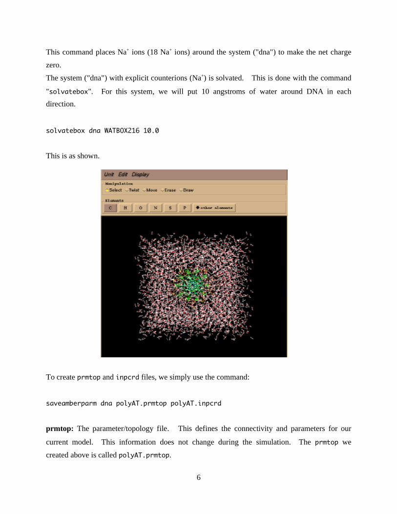
This command places Na+ ions (18 Na+ ions) around the system ("dna") to make the net charge

zero.

The system ("dna") with explicit counterions (Na+) is solvated. This is done with the command

"solvatebox". For this system, we will put 10 angstroms of water around DNA in each

direction.

solvatebox dna WATBOX216 10.0

This is as shown.

To create prmtop and inpcrd files, we simply use the command:

saveamberparm dna polyAT.prmtop polyAT.inpcrd

prmtop: The parameter/topology file. This defines the connectivity and parameters for our

current model. This information does not change during the simulation. The prmtop we

created above is called polyAT.prmtop.

7

inpcrd: The coordinates (and box coordinates, if present and optionally the velocities). This

changes during simulation. Above we created an initial set of coordinates called

polyAT.inpcrd.

Now you can go on to the next section which introduces us to running molecular dynamics and

minimization.

8

3. Equilibration.After you have built up the structure, you are ready to begin minimization and molecular

dynamics simulations to equilibrate the system.

The procedure of the minimization and molecular dynamics simulations are shown as follows.

A. Minimization holding the solute (DNA) fixed

A short minimization run to remove any potentially bad contacts between solute and

solvent molecules.

B. Dynamics holding the solute (DNA) fixed

The bulk of the water relaxation takes place. Minimization does not really sample the

accessible conformational space of the water.

C. Moving the DNA

We gradually reduce the restraints on the DNA in a series of minimizations.

D. Equilibration of the DNA

The DNA model is equilibrated by a 20 ps molecular dynamics simulation.

A. Minimization holding the solute (DNA) fixed

Given our prmtop (polyAT.prmtop) and inpcrd (polyAT.inpcrd) we created, we will now use

sander in a short minimization run, with position restraints, to remove bad interactions between

solute and solvent.

The basic usage for sander is as follows:

sander [-O] -i mdin -o mdout -p prmtop -c inpcrd -r restrt

[-ref refc -x mdcrd -v mdvel -e mden -inf mdinfo]

Arguments in []'s are optional.

If an argument is not specified, the default name will be used.

-O overwrite all the output files

-i the name of the input file, mdin by default

-o the name of the output file, mdout by default

-p the parameter/topology file, prmtop by default

-c the set of initial coordinates for this run, inpcrd by default

-r the final set of coordinates from this MD or minimization run, restrt by default

9

-ref reference coordinates for positional restraints, if this option is specified in the input file,

refc by default

-x the molecular dynamics trajectory (if running MD), mdcrd by default

-v the molecular dynamics velocities (if running MD), mdvel by default

-e a summary file of the energies (if running MD), mden by default

-inf a summary file written every time energy information is printed in the output file for the

current step of the minimization or MD, mdinfo by default

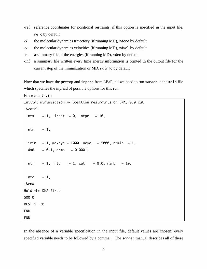
Now that we have the prmtop and inpcrd from LEaP, all we need to run sander is the mdin file

which specifies the myriad of possible options for this run.

File min_ntr.in

Initial minimization w/ position restraints on DNA, 9.0 cut

&cntrl

ntx = 1, irest = 0, ntpr = 10,

ntr = 1,

imin = 1, maxcyc = 1000, ncyc = 5000, ntmin = 1,

dx0 = 0.1, drms = 0.0001,

ntf = 1, ntb = 1, cut = 9.0, nsnb = 10,

ntc = 1,

&end

Hold the DNA fixed

500.0

RES 1 20

END

END

In the absence of a variable specification in the input file, default values are chosen; every

specified variable needs to be followed by a comma. The sander manual describes all of these

10

inputs, for each of the possible namelists. Which namelist is used depends on the specification

above, such as &cntrl. At minimum, the &cntrl namelist must be specified. Also notice the

space or empty first column before specification of the namelist control variable; this is necessary.

It is also necessary to end each namelist with &end. After the namelist, some other information

may be specified, such as "GROUP" input, which allows atom selections for restraints.

Now, let us build up a minimal input file for performing minimization with position restraints on

the DNA atoms. Here are things to notice in the input file:

The first part shows the format of output.

ntx = 1:

The initial coordinates are read formatted with no initial velocity information (default)

irest = 0:

This is not a continuation of a previous dynamics run.

ntpr = 10:

Every 10 steps energy information will be printed in human-readable form to files

"mdout". Default is 50.

The second part shows the restraint of this calculation.

ntr = 1:

This means that we have turned on position restraints and therefore have to specify via

GROUP input the atoms which are restrained as well as the force constant. In this

example, after specification of the namelists, a title is given, followed by the force

constant for the restraint (in kcal mol–1 angstrom–2) and then a specification of residues

or atoms to restrain. Residues can be specified using the "RES" keyword. We have

chosen a force constant of 500 kcal mol–1 angstrom–2 and restrained residues 1 through

20.

The third part shows the minimization regulation.

imin = 1:

Minimization is turned on.

maxcyc = 1000, ncyc > maxcyc; for example ncyc = 5000:

This means that we will be running 1000 steps of steepest descent minimization.

Conjugate gradient minimization typically fails with rigid water (TIP3P). So by keeping

ncyc > maxcyc we never changes the method of minimization from steepest descent to

11

conjugate gradient method.

dx0 = 0.1:

The initial step length. Default is 0.01.

drms = 0.0001:

Convergence criterion for the energy gradient. Default 0.0001 kcal mol–1 Å–1.

The fourth part controls a molecular dynamics.

ntf =1:

Complete interaction is calculated. (default)

ntb = 1:

Periodic boundary is applied under constant temperature.

cut = 9.0:

We are running with a 9 angstrom cutoff

nsnb = 10:

Updating the pairlist every 10 steps.

The last part indicates SHAKE regulation.

ntc = 1,

SHAKE is not performed. (default)

SHAKE

When the simulation involves conformationally flexible molecules such as proteins then the high

frequency motions (e.g. bond vibrations) are usually of less interest than the lower frequency

modes, which often correspond to major conformational changes. Unfortunately, the time step

of a molecular dynamics simulation is dictated by the highest frequency motion present in the

system. It would therefore be of considerable benefit to be able to increase the time step

without prejudicing the accuracy of the simulation. Constraint dynamics enables individual

internal coordinates or combinations of specified coordinates to be constrained, or 'fixed' during

the simulation without affecting the other internal degrees of freedom. The most commonly

used method for applying constraints is the SHAKE procedure.

To run the minimization, we should make cmd file (min_ntr.cmd) and submit this file to the

queue system using qsub. The min_ntr.cmd file is shown as follows:

12

file min_ntr.cmd

#PBS -S/bin/bash

#PBS -l pmem=200mb

#PBS -l nodes=1:m200mb

#PBS -N min_ntr

cd /users1/$USER/TUTORIAL

export AMBERHOME='/usr/local/amber7'

export PATH=$PATH:/usr/local/amber7/exe

wait

/usr/local/amber7/exe/sander -O -i min_ntr.in -o min_ntr.out -c polyAT.inpcrd ¥

-p polyAT.prmtop -r min_ntr.restrt -ref polyAT.inpcrd

wait

[Note: the "¥" in the lines above are just continuations for the shell to allow you to type over

multiple lines. When you actually type this in, just type it in on one command line.]

The command to run the minimization is as follows:

qsub min_ntr.cmd

Input files: min_ntr.in, polyAT.inpcrd, polyAT.prmtop

Output files: min_ntr.out, min_ntr.restrt

B. Dynamics holding the solute (DNA) fixed

Using the restrt file generated from the previous step (min_ntr.restrt), we now run

dynamics, holding the DNA fixed with positional restraints. This is where the bulk of the water

relaxation takes place. Minimization does not really sample the accessible conformational space

of the water; it simply serves to move the energy down hill. Large "moves" or changes in the

coordinates are not possible. During the dynamics on the other hand, the water is free to move

around (subject to the kinetic energy or temperature supplied to the system initially) and also the

box size is changing in an attempt to maintain constant pressure.

13

file md_ntr.in

5DNB, initial dynamics w/ belly on DNA, model1, 9.0 cut

&cntrl

nmropt = 1,

ntx = 1, irest = 0, ntpr = 100, ntwx = 500,

ntf = 2, ntb = 2, cut = 9.0, nsnb = 10,

ntr = 1,

imin = 0, nstlim = 25000, nscm = 0, dt = 0.001,

temp0 = 300.0, tempi = 100.0, ig = 71277,

ntt = 1, tautp = 0.2, vlimit = 15.0,

ntp = 1, pres0 = 1.0, comp = 44.6, taup = 0.2,

ntc = 2, tol = 0.00001,

&end

&wt

type='TEMP0', istep1=0, istep2=1000,

value1=100.0, value2=300.0,

&end

&wt


value1=300.0, value2=300.0,

&end

&wt

type='END',

&end

&rst

iat=0,

&end

Hold the DNA fixed

500.0

RES 1 20

END

END

14

In this run, minimization is turned off (imin = 0) and dynamics can now proceed (for nstlim

steps). In addition to this change in the input file, there are a few other major differences:

nmropt = 1:

We are going to use some of the "NMR" options. This is just to control temperature.

We want to start the temperature off at 100 K and then ramp it up to 300 K. This is

done with the &wt to &end namelists.

&wt


value1=100.0, value2=300.0,

&end

Over 1000 steps raise the temperature from 100.0 to 300.0 K.

&wt


value1=300.0, value2=300.0,

&end

Over the next 24000 steps, keep the temperature at 300 K.

Do not forget that you need to terminate the &rst namelist even if you are not specifying

NMR restraints. This is then followed by the same group input as before.

ntwx = 500:

Every 500 steps the coordinates will be written to file "mdcrd". Default is 0.

ntf = 2:

Bond interactions involving H-atoms omitted. (use with ntc = 2)

ntb = 2:

Periodic boundary is applied under constant pressure.

nstlim = 25000, dt = 0.001:

We are running 25000 steps at a time step of 1 femtosecond. This implies a total

simulation of 25 picoseconds.

ntt = 1, tautp = 0.2:

We use standard temperature coupling (ntt = 1) to keep the temperature with 0.2ps of

time constant for heat bath coupling for the system (tautp = 0.2). The default of

tautp is 1.0.

15

temp0 = 300.0:

The simulation keeps the temperature at 300.0 K. Default is 300.0 K.

tempi = 100.0:

The initial temperature (tempi = 100.0) to make the initial distribution. Default is

300.0 K.

ig = 71277:

The random number generator seed. Note that the initial distribution of temperatures is

dependent on ig; in other words, every time you run with ig = 71277 on the same

system, you will get the same distribution of initial velocities.

vlimit = 15.0:

Any component of the velocity that is greater than abs(vlimit) will be reduced to

vlimit (preserving the sign).

ntp = 1:

In "constant pressure" dynamics, the volume of the unit cell is adjusted (by small

amounts on each step) to make the computed pressure approach the target pressure,

pres0. This dynamics is performed with isotropic position scaling.

pres0 = 1.0:

Reference pressure ( in units of bars, where 1 bar ~ 1 atm) at which the system

maintained. Default is 1.0.

comp = 44.6:

Compressibility of the system. The units are in 0.000001 bar; a value of 44.6 (default)

is appropriate for water.

taup = 0.2:

Pressure relaxation time (in ps). Default value of 0.2 could be used for equilibration to

more quickly get the desired density.

ntc = 2, tol = 0.00001:

SHAKE on hydrogens is now turned on. This is necessary when using rigid water

models such as TIP3P. The SHAKE tolerance is 0.00001.

16

file md_ntr.cmd

#PBS -S/bin/bash

#PBS -l pmem=200mb


#PBS -N md_ntr




wait

/usr/local/amber7/exe/sander -O -i md_ntr.in -o md_ntr.out -c min_ntr.restrt ¥

-p polyAT.prmtop -r md_ntr.restrt -ref min_ntr.restrt -x md_ntr.mdcrd

wait

The command to run the dynamics is as follows:

qsub md_ntr.cmd

Input files: md_ntr.in, min_ntr.restrt, polyAT.prmtop

Output files: md_ntr.out, md_ntr.restrt, md_ntr.mdcrd

C. Moving the DNA

All throughout the previous steps, the DNA was held relatively rigid. Now we gradually reduce

the restraints on the DNA in a series of minimizations.

The basic plan is

1) 1000 steps minimization with 25.0 kcal mol–1 angstrom–2 position restraints on the DNA;

(equil_min1)

2) 600 steps minimization, reducing the positional restraints by 5.0 kcal mol–1 angstrom–2 each

run; (equil_min2 (20.0 kcal mol–1 angstrom–2) — equil_min6 (0.0 kcal mol–1 angstrom–2))

Since you already have all the machinery necessary to follow through, details are not shown.

Actual cmd and input files are shown as follows. (equil_min1 — equil_min6)

17

file equil_min1.in

5DNB, equil step 1

&cntrl

ntx = 1, irest = 0, ntpr = 500,

ntf = 1, ntb = 1, cut = 9.0, nsnb = 10,

ntr = 1,

imin = 1, maxcyc = 1000, ncyc = 5000,

ntmin = 1, dx0 = 0.1, drms = 0.0001,

ntc = 1,

&end

Constraints

22225555....0000

RES 1 20

END

END

file equil_min1.cmd

#PBS -S/bin/bash

#PBS -l pmem=200mb


#PBS -N equil_min1




wait

/usr/local/amber7/exe/sander -O -i equil_min1.in -o equil_min1.out ¥

-c md_ntr.restrt -p polyAT.prmtop ¥

-r equil_min1.restrt -ref md_ntr.restrt ¥

wait

qsub equil_min1.cmd

18

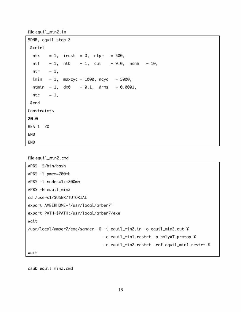
file equil_min2.in

5DNB, equil step 2

&cntrl

ntx = 1, irest = 0, ntpr = 500,

ntf = 1, ntb = 1, cut = 9.0, nsnb = 10,

ntr = 1,

imin = 1, maxcyc = 1000, ncyc = 5000,

ntmin = 1, dx0 = 0.1, drms = 0.0001,

ntc = 1,

&end

Constraints

22220000....0000

RES 1 20

END

END

file equil_min2.cmd

#PBS -S/bin/bash

#PBS -l pmem=200mb


#PBS -N equil_min2




wait


-c equil_min1.restrt -p polyAT.prmtop ¥

-r equil_min2.restrt -ref equil_min1.restrt ¥

wait

qsub equil_min2.cmd

19

file equil_min3.in

5DNB, equil step 3

&cntrl

ntx = 1, irest = 0, ntpr = 500,

ntf = 1, ntb = 1, cut = 9.0, nsnb = 10,

ntr = 1,

imin = 1, maxcyc = 1000, ncyc = 5000,

ntmin = 1, dx0 = 0.1, drms = 0.0001,

ntc = 1,

&end

Constraints

11115555....0000

RES 1 20

END

END

file equil_min3.cmd

#PBS -S/bin/bash

#PBS -l pmem=200mb


#PBS -N equil_min3




wait




wait

qsub equil_min3.cmd

20

file equil_min4.in

5DNB, equil step 4

&cntrl

ntx = 1, irest = 0, ntpr = 500,

ntf = 1, ntb = 1, cut = 9.0, nsnb = 10,

ntr = 1,

imin = 1, maxcyc = 1000, ncyc = 5000,

ntmin = 1, dx0 = 0.1, drms = 0.0001,

ntc = 1,

&end

Constraints

11110000....0000

RES 1 20

END

END

file equil_min4.cmd

#PBS -S/bin/bash

#PBS -l pmem=200mb


#PBS -N equil_min4




wait




wait

qsub equil_min4.cmd

21

file equil_min5.in

5DNB, equil step 5

&cntrl

ntx = 1, irest = 0, ntpr = 500,

ntf = 1, ntb = 1, cut = 9.0, nsnb = 10,

ntr = 1,

imin = 1, maxcyc = 1000, ncyc = 5000,

ntmin = 1, dx0 = 0.1, drms = 0.0001,

ntc = 1,

&end

Constraints

5555....0000

RES 1 20

END

END

file equil_min5.cmd

#PBS -S/bin/bash

#PBS -l pmem=200mb


#PBS -N equil_min5




wait




wait

qsub equil_min5.cmd

22

file equil_min6.in

5DNB, equil step 6

&cntrl

ntx = 1, irest = 0, ntpr = 500,

ntf = 1, ntb = 1, cut = 9.0, nsnb = 10,

ntr = 1,

imin = 1, maxcyc = 1000, ncyc = 5000,

ntmin = 1, dx0 = 0.1, drms = 0.0001,

ntc = 1,

&end

file equil_min6.cmd

#PBS -S/bin/bash

#PBS -l pmem=200mb


#PBS -N equil_min6




wait



-r equil_min6.restrt ¥

wait

qsub equil_min6.cmd

23

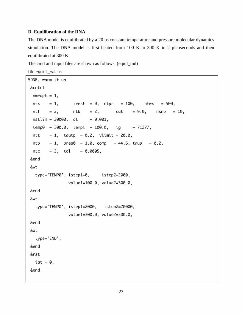
D. Equilibration of the DNA

The DNA model is equilibrated by a 20 ps constant temperature and pressure molecular dynamics

simulation. The DNA model is first heated from 100 K to 300 K in 2 picoseconds and then

equilibrated at 300 K.

The cmd and input files are shown as follows. (equil_md)

file equil_md.in

5DNB, warm it up

&cntrl

nmropt = 1,

ntx = 1, irest = 0, ntpr = 100, ntwx = 500,

ntf = 2, ntb = 2, cut = 9.0, nsnb = 10,

nstlim = 20000, dt = 0.001,

temp0 = 300.0, tempi = 100.0, ig = 71277,

ntt = 1, tautp = 0.2, vlimit = 20.0,

ntp = 1, pres0 = 1.0, comp = 44.6, taup = 0.2,

ntc = 2, tol = 0.0005,

&end

&wt


value1=100.0, value2=300.0,

&end

&wt


value1=300.0, value2=300.0,

&end

&wt

type='END',

&end

&rst

iat = 0,

&end

24

file equil_md.cmd

#PBS -S/bin/bash

#PBS -l pmem=200mb


#PBS -N equil_md




wait

/usr/local/amber7/exe/sander -O -i equil_md.in -o equil_md.out ¥


-r equil_md.restrt -x equil_md.mdcrd ¥

wait

qsub equil_md.cmd

Input files: equil_md.in, equil_min6.restrt, polyAT.prmtop

Output files: equil_md.out, equil_md.restrt, equil_md.mdcrd

25

4. Analyzing results.

After equilibrating the system by a molecular dynamics simulation, we should analyze the

simulated results from a molecular dynamics run using some of the tools supplied within

AMBER and some available through other sources.

Creating pdb files from the AMBER coordinates files

You may want to generate a new pdb file so you can look at the structure using the minimized

coordinates from restrt. The pdb can be created from the parm topology and coordinates

(inpcrd or restrt) using the program ambpdb.

ambpdb -p polyAT.prmtop < equil_md.restrt > equil_md.pdb

This will take the prmtop and inpcrd (polyAT.prmtop and equil_md.restrt) specified and

create the file (equil_md.pdb).

Extracting the energies, etc. from the mdout file

If you want to pull out the energies, etc. directly from mdout file, you can write an awk, sed, or

perl script or use a perl script prepared in the AMBER web page.

process_mdout.perl equil_md.out

This script will take a whole series of mdout files and will create a whole series, leading off with

the prefix "summary." such as "summary.ETOT". These files are just columns of times vs. the

value for each of the energy components. You can plot this with a program.

26

Here is the total energy (ETOT) as a function of time (20 ps):

-55000

-50000

-45000

-40000

-35000

-30000

0 5 1 0 1 5 2 0

Tot

al E

nerg

y / k

cal m

ol-1

Time / ps

27

Calculating the RMS deviation vs. time

To calculate the RMS deviation as a function of time, we can use carnal or ptraj. In ptraj,

this is done with the list of commands specified in the file calc_rms.1.

ptraj polyAT.prmtop < calc_rms.1

Input files: polyAT.prmtop, equil_md.mdcrd, calc_rms.1

Output file: rms.1

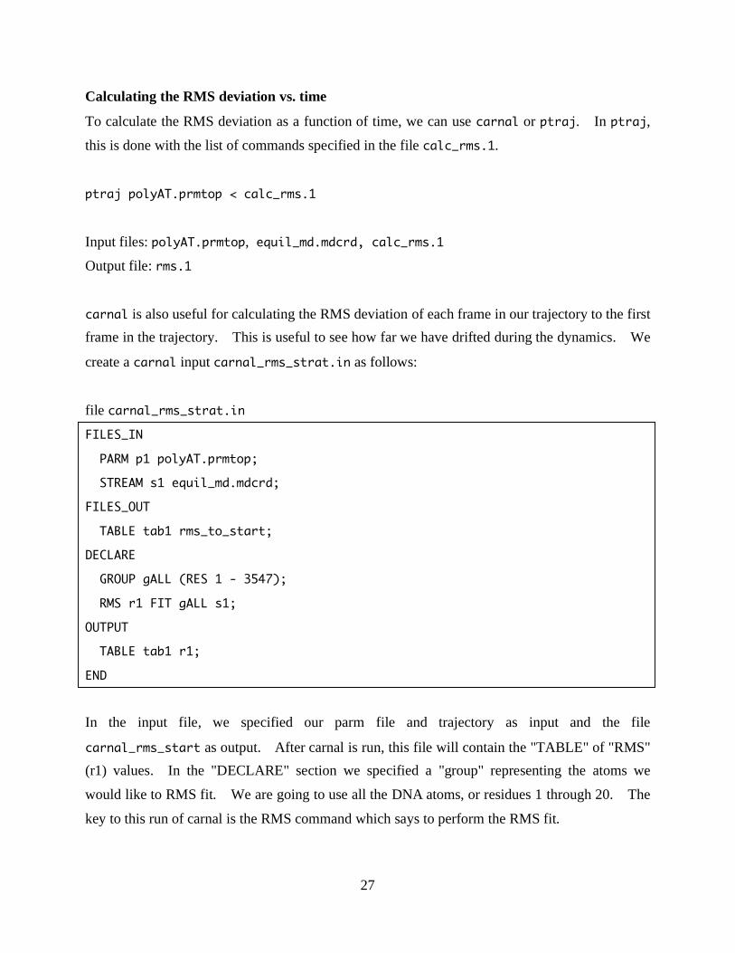
carnal is also useful for calculating the RMS deviation of each frame in our trajectory to the first

frame in the trajectory. This is useful to see how far we have drifted during the dynamics. We

create a carnal input carnal_rms_strat.in as follows:

file carnal_rms_strat.in

FILES_IN

PARM p1 polyAT.prmtop;

STREAM s1 equil_md.mdcrd;

FILES_OUT

TABLE tab1 rms_to_start;

DECLARE

GROUP gALL (RES 1 - 3547);

RMS r1 FIT gALL s1;

OUTPUT

TABLE tab1 r1;

END

In the input file, we specified our parm file and trajectory as input and the file

carnal_rms_start as output. After carnal is run, this file will contain the "TABLE" of "RMS"

(r1) values. In the "DECLARE" section we specified a "group" representing the atoms we

would like to RMS fit. We are going to use all the DNA atoms, or residues 1 through 20. The

key to this run of carnal is the RMS command which says to perform the RMS fit.

28

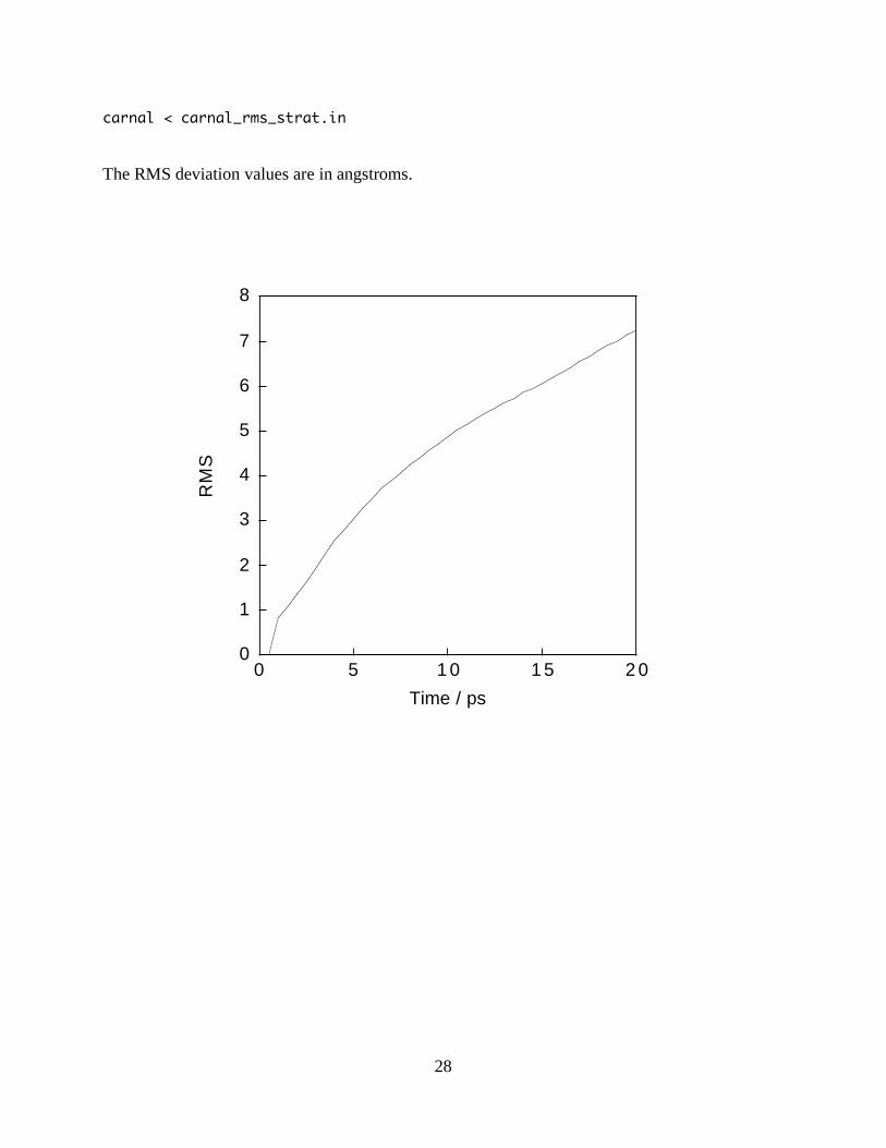
carnal < carnal_rms_strat.in

The RMS deviation values are in angstroms.

0

1

2

3

4

5

6

7

8

0 5 1 0 1 5 2 0

RM

S

Time / ps

29

Measuring atomic positional fluctuations with carnal

Note that carnal can also calculating atomic positional fluctuations which are directly related to

the atomic B-factors.

The calculation is a two-step procedure, running carnal twice. In the first step you calculate the

average structure of the trajectory. In the second step the RMS distances between the averaged

structure and the trajectory is calculated.

carnal < carnal_fluctuation1

carnal < carnal_fluctuation2 > fluctuation

Here is the atomic positional fluctuations of the solute (DNA model).

0

2

4

6

8

1 0

1 2

0 100 200 300 400 500 600 700

RM

S

ATOM

amber tutorial - ucla chemistry and biochemistrymccarren/tutorials/ambertutorial.pdf1 amber tutorial...

Documents