ambiguity preferences and portfolio choices: … preferences and portfolio choices: evidence from...

Ambiguity Preferences and Portfolio Choices:Evidence from the Field∗

Milo Bianchi† Jean-Marc Tallon‡

November 7, 2017

Abstract

We match administrative panel data on portfolio choices with sur-vey data on preferences over ambiguity. We show that ambiguity averseinvestors bear more risk, due to a lack of diversification. In particu-lar, they exhibit a form of home bias that leads to higher exposure tothe domestic relative to the international stock market. While moresensitive to market factors, their returns are on average higher, sug-gesting that ambiguity averse investors need not be driven out of themarket for risky assets. We also show that these investors rebalancetheir portfolio more actively and in a contrarian direction relative topast market trends, which allows them to keep their risk exposure rel-atively constant over time. We discuss these findings in relation to thetheoretical literature on portfolio choice under ambiguity.

∗We are grateful to Han Bleichrodt (editor), an associate editor and two referees forvery constructive comments. We also thank Marianne Andries, Luc Behaghel, BrunoBiais, Luigi Guiso, Roy Kouwenberg, David Margolis, David Schroeder, Bernard Salanié,Paul Smeets, Vassili Vergopoulos, Peter Wakker and various seminar participants for veryuseful discussions, and Henri Luomaranta for excellent research assistance. Financialsupport from AXA Research Fund and from the Amundi, Groupama and Scor Chairs isgratefully acknowledged.†Toulouse School of Economics, University of Toulouse Capitole, Toulouse, France.

E-mail: [email protected]‡Paris School of Economics, CNRS. E-mail: [email protected]

1

1 Introduction

Ambiguity has been widely studied both theoretically and experimentallyin the past decades. Its implications have been investigated in a variety ofsettings, including financial behaviors.1 It is now commonly understood, atleast at an intuitive level, that ambiguity is an important element that house-holds face in their financial decisions (Ryan, Trumbull and Tufano (2011),Guiso and Sodini (2013)). It may also be a key ingredient to explain thefunctioning of financial markets.2 Field evidence of how ambiguity affectshouseholds is however still very scarce:

Interestingly, the empirical literature has so far provided little ev-idence linking individual attitudes toward ambiguity to behavioroutside the lab. Are those agents who show the strongest degreeof ambiguity aversion in some decision task also the ones whoare most likely to avoid ambiguous investments? (Trautmannand Van De Kuilen (2015))

This paper attempts to partially fill this gap. We explore the relationbetween ambiguity aversion and portfolio choices using a unique data setthat matches administrative panel data on portfolio choices with surveydata on preferences over ambiguity.

We have obtained portfolio data from a large financial institution inFrance. We focus on a popular investment product among French house-holds dubbed assurance vie. In this product, households decide their portfo-lio weight on relatively safe assets (essentially bundles of bonds, called eurofunds) vs. relatively risky assets (essentially mutual funds, called uc funds)as well as some features of risky assets (such as their exposure to the do-mestic vs. international stock markets). Households can freely change theirportfolios over time. Our data record the clients’portfolio of these contractsat a monthly frequency for about nine years. Moreover, for each portfolio,we can construct the corresponding returns.

Clients were also asked to answer a survey that we have designed and thatserves two main purposes. First, while portfolio data only concern house-holds’activities within the company, in the survey we gather a more com-

1See, e.g., Etner, Jeleva and Tallon (2012), Machina and Siniscalchi (2014), Gilboa andMarinacci (2013) for surveys of the various models, and Hey (2014) or Trautmann and VanDe Kuilen (2015) for surveys of the experimental literature. Closely related experimentalevidence is provided in Ahn, Choi, Gale and Kariv (2014), who study how ambiguityaversion affects portfolio choices, and in Bossaerts, Ghirardato, Guarnaschelli and Zame(2010), who focus on its effects on asset prices.

2Epstein and Schneider (2010) and Guidolin and Rinaldi (2013) provide recent insight-ful reviews on ambiguity and financial choices. Macro-finance applications include Uppaland Wang (2003), Ju and Miao (2012), Collard, Mukerji, Sheppard and Tallon (2012).On the role of ambiguity in financial crises, see e.g. Caballero and Krishnamurthy (2008)and Caballero and Simsek (2013).

2

plete picture of households’portfolios as well as various socio-demographicdata. Second, we elicit a number of behavioral traits, and in particularhouseholds’ attitudes towards ambiguity. Following standard procedures,we build our main measure of ambiguity aversion by asking subjects tochoose between lotteries with known vs. unknown probability distributionsover the final payoffs.

Guided by some fundamental insights developed in the theoretical lit-erature of portfolio choices under ambiguity, we focus on three dimensionsof household portfolios. We first look at how the composition of portfo-lios varies with ambiguity aversion. Is it the case that ambiguity aversionleads to a form of under-diversification, as predicted for example in Uppaland Wang (2003) and Hara and Honda (2016)? In particular, do ambiguityaverse investors display a preference for home stocks, as in Boyle, Garlappi,Uppal and Wang (2012)?

Second, we ask whether ambiguity averse households display distinctportfolio returns. Are their returns systematically lower, so that in the longrun these investors are bound to be wiped out of the market, as in Condie(2008)? At the same time, in relation to under-diversification, are theirreturns more volatile?

Third, we analyze the relation between ambiguity aversion and portfoliodynamics. In particular, as suggested by recent models on portfolio inertia(Garlappi, Uppal and Wang (2007), Illeditsch (2011)), is it the case thatambiguity averse households keep their portfolio weights more stable overtime?

In terms of portfolio composition, we find that ambiguity averse investorsare more exposed to risk, as defined both in terms of the volatility of returnsand in terms of beta relative to the French stock market. This extra expo-sure to risk could come, as suggested for instance by Klibanoff, Marinacciand Mukerji (2005), from a desire to shy away from ambiguity. To pursuethis line, we distinguish portfolios according to their relative exposure tothe French and the world markets. We build a measure of differential expo-sure based on the difference between a "domestic" beta -which employs asbenchmark the French stock market index CAC40- and an "international"beta -which instead uses as benchmark the MSCI World Index. We showthat ambiguity averse investors are relatively more exposed to the Frenchthan to the international stock market. Ambiguity aversion is thus a goodcandidate to explain home bias in equity markets.

We also study the extent to which portfolio returns are explained bysimple asset pricing models, and in particular by a domestic CAPM andby the Fama-French five-factor model. In both specifications, we find thatthe higher ambiguity aversion, the lower is the explanatory power of mar-ket factors. Ambiguity averse investors appear to bear more idiosyncraticvolatility, suggesting a possible under-diversification in their portfolios.

3

We then look at portfolio returns. We find that, in our sample, ambigu-ity averse investors experience higher returns, even controlling for standardmeasures of risk. At the same time, however, their returns are more sensitiveto market trends. Our estimates show that the larger ambiguity aversion,the higher are returns in good times and the lower are returns in bad times.

A similar picture emerges as we explore the differential exposure of am-biguity averse investors to Fama-French factors. These investors experiencerelatively higher returns when returns of the market portfolio are high, evenmore so when we construct market returns based only on the French stockmarket. Moreover, we show that ambiguity averse investors are more ex-posed to the Fama-French investment factor; that is, their portfolios loadmore on firms with "conservative" as opposed to "aggressive" investmentstrategies.

Finally, we investigate the dynamics of household portfolios. In partic-ular, we focus on how households’risky share, as measured by the share ofuc funds in their portfolios, evolves over time. Following the methodologydeveloped in Calvet, Campbell and Sodini (2009), we distinguish changesin risk exposure which are driven by differential returns of risky vs. risklessassets from those which result from an active choice of the household. Weshow that ambiguity averse investors tend to rebalance their portfolio moreactively; that is, their risky share tends to remain closer to the target share.Furthermore, we show that ambiguity averse investors adopt a contrarianstrategy, moving wealth from funds which have experienced relatively higherreturns to those who had relatively lower returns. This rebalancing strategyaims at keeping the risky share relatively constant over time, which is inline with the above mentioned models of ambiguity aversion and portfolioinertia.

In the next sections we discuss each of these findings and we highlight inmore details their relation with the existing theoretical literature. From asomewhat broader perspective, we believe these insights contribute to a bet-ter understanding of the empirical content of ambiguity preferences. Whilefrom a conceptual viewpoint the importance of ambiguity has been recog-nized at least since Knight (1921), its empirical content is still unclear. Inhis Nobel lecture, Hansen (2014) calls for further research aimed at assessingwhether ambiguity, in addition to risk, is empirically relevant for the studyof asset pricing. Our results are strongly suggestive that ambiguity aversionis an important determinant of observed financial outcomes. We believethey should serve as motivation for further work aimed at distinguishingmore clearly risk from ambiguity both in investors’perceptions and in theirfinancial behavior.

4

Related Literature

To our knowledge, this study is the first to provide evidence on the effect ofambiguity aversion on financial outcomes observed in administrative data.As such, it relates, from an empirical angle, to the mostly theoretical liter-ature that has studied the implications of ambiguity aversion for portfoliochoices and financial markets.3

We also contribute to the household finance literature by looking at thedeterminants of households’financial decisions. The literature is growingrapidly and we refer to Campbell (2006) and Guiso and Sodini (2013) forrecent surveys. Compared to this literature, our main novelty is in matchingsurvey and administrative data. While as pointed out our data do not pro-vide a detailed picture of the entire households’portfolios (as for example inCalvet, Campbell and Sodini (2007) and Calvet et al. (2009)), they offer theopportunity to study the relation between behavioral traits and the choicestaken within the company. The latter allows us to address quantitativeissues that purely survey data usually cannot address.

We know of only a few studies combining survey and administrative data.Dorn and Huberman (2005) focus on the relation between risk aversion,(perceived) financial sophistication and portfolio choices; Alvarez, Guiso andLippi (2012) analyze the frequency with which investors observe and tradetheir portfolio; Guiso, Sapienza and Zingales (2017) and Hoffmann, Post andPennings (2013) study how risk aversion has changed following the financialcrisis; Bauer and Smeets (2015) and Riedl and Smeets (2014) investigatehow social preferences affect socially responsible investments. None of thesestudies focuses on ambiguity preferences as we do.

Most closely related to our study, Dimmock, Kouwenberg and Wakker(2016) and Dimmock, Kouwenberg, Mitchell and Peijnenburg (2016) exploitlarge representative surveys in which subjects are asked about their prefer-ences over ambiguity as well as about their portfolio holdings. We share withthese authors a similar methodology to elicit ambiguity aversion (althoughour subjects receive no monetary reward in relation to their choices) butthe nature of our data, and so the questions we address, are quite different.Their data are based on surveys, and they are larger in size and in scope.This allows them to investigate issues of stock market participation whichwe cannot address. Our data provide more details on the investment prod-uct at hand as well as a panel structure, and this allows us to investigatequestions on portfolio dynamics and returns which cannot be addressed withtheir data.

Dimmock, Kouwenberg, Mitchell and Peijnenburg (2016) also point at

3Recent developments include Gollier (2011) on the comparative statics of ambiguityaversion in portfolio choices; Maccheroni, Marinacci and Ruffi no (2013) on mean-variancepreferences; Hara and Honda (2016) on CARA smooth ambiguity preferences; Epsteinand Ji (2013) and Lin and Riedel (2014) on dynamic portfolio choices.

5

a positive relation between ambiguity aversion and lack of portfolio diver-sification. We complement their findings by documenting forms of under-diversification starting from information about realized portfolio returns asopposed to stock holding. This allows to highlight how under-diversificationaffects the riskiness of household portfolios, and to provide support for theidea that ambiguity averse investors tend to bear more risk so as to avoidambiguity, consistently with different models in the literature (see Section 4for details).

2 Data

We exploit three sources of data. First, we have obtained data on portfoliochoices from a large French financial institution. These data describe clients’holdings of assurance vie contracts. These are investment products widelyused in France; they are the most common way through which householdsinvest in the stock market.4 A typical assurance vie contract establishes thetypes of funds in which the household wishes to invest and the amount ofwealth allocated to each fund.

A first key distinction is between euro funds and uc funds. The first typeof assets, which are called euro funds, are basically bundles of bonds. Thecapital invested in these funds is guaranteed by the company. The secondtype of funds are called uc funds, and they are essentially bundles of stocks.It is made clear to investors that uc funds tend to provide larger expectedreturns and larger risk. Investors do not observe the exact composition ofthese funds (neither do we), but they receive some information about theintended risk profile of these funds (e.g. conservative vs. aggressive) as wellas an indication of their exposure to different markets. A particularly salientfeature is whether funds invest in domestic, emerging, or world markets.

Over time, clients are free to change the composition of their portfolios,make new investment and withdraw money as they wish.5 Investors may optfor automatic rebalancing of their portfolio according to some pre-specifiedrule. In our sample, less than 10% of investors have chosen this option (seethe Online Appendix for further details).

Our portfolio data records at a monthly frequency the value and compo-sition of these contracts for 511 clients from September 2002 to April 2011.These data are combined with the responses to a survey we have designed

4According to the French National Institute for Statistics, 41% of French householdsheld at least one of these contracts in 2010. This makes it the most widespread financialproduct after Livret A, a saving account whose returns are set by the state. See INSEEPremiere n. 1361 - July 2011 (http://www.insee.fr/fr/ffc/ipweb/ip1361/ip1361.pdf).

5A specific feature of the product is that there is some incentive not to liquidate thecontract before some time (8 years in our sample period) so as to take advantage of reducedtaxes on capital gains. We show in the Online Appendix that this feature is immaterialfor our results.

6

and which was administered by a professional survey company at the end of2010.6

The financial institution has provided to the survey company a sampleof clients who had an account open at the end of 2010. The survey was thenimplemented in order to obtain a representative sample of French householdsin terms of family status, employment status, sector of employment, revenues(these characteristics follow offi cial classifications of the National Institutefor Statistics).7 All clients in our sample held some assurance vie contractin the financial company at the time when the survey was conducted, butnot necessarily throughout the entire sample period.8

These contracts can represent a sizeable fraction of households’finan-cial wealth. In our sample, the average value of a portfolio is 32, 700 euros,the maximum is 590, 000 euros. The median total wealth in our sampleis between 225 and 300 thousand euros and the median financial wealth isbetween 16 and 50 thousands euros. These figures are in line with those ob-tained for the general French population (see Arrondel, Borgy and Savignac(2012)).9

The survey serves two main purposes: first, we have gathered informationabout demographic characteristics, wealth and portfolio holdings outside thecompany. In this way we can control for a richer set of clients’characteristicsthan those recorded by the company. Moreover, this allows to gauge whetherthe behaviors we observe within the company are informative for clients’behaviors in their overall portfolio (see the Online Appendix for details).

A second purpose of the survey is to get an idea of clients’behavioralcharacteristics, and in particular of their preferences over ambiguity. In thenext section, we describe how we have elicited these preferences.10

Finally, we collected data on portfolio returns. We have obtained fromThomson Reuters Datastream the returns experienced in a given month by

6 It was made clear to the subjects that they were contacted as part of a scientificproject on risk, while the insurance company was never mentioned during the interview.Clients completed the survey over the internet while on line with the surveyor.

7The insurance company gave to the survey company a sample of approximately 30,000clients. This sample was stratified according to geographic regions (Ile De France, North-East, West, South-East, South-West) and the survey was conducted so as to meet pre-specified quotas of respondents in terms of the above-mentioned socio-demographic char-acteristics.

8We did not impose any minimal holding period to be included in the sample. Wediscuss in the Online Appendix a series of robustness checks to address the possibility ofsurvivorship bias in this sample.

9For offi cial and comprehensive data, see the 2010 HouseholdWealth Survey from the French National Institute for Statistics(http://www.insee.fr/en/methodes/default.asp?page=sources/ope-enquete-patrimoine.htm).10Our measure of ambiguity aversion is taken just at one point in time, towards the

end of the sample period. In the Online Appendix, we show that the effects of ambiguityaversion would be similar if we were to restrict our analysis to the beginning of the sampleperiod. This suggests that our measure of ambiguity aversion has a persistent component.

7

each fund and, based on those, we can build the corresponding returns ofeach contract.

3 Ambiguity Preferences

We elicit preferences over ambiguity in a classical way. We ask respondentsto choose between a risky lottery and an ambiguous lottery. For the formerlottery, we provide an exact probability distribution over the final payoffs;for the latter, we provide no information about the probabilities associatedto the final payoffs. Depending on their answer, we sequentially providealternative lotteries in which the risky lottery is made relatively more orless attractive. We describe these lotteries in details in the Appendix.

This approach is in line with the results in Dimmock, Kouwenberg andWakker (2016), who formally show that ambiguity attitudes can be entirelydescribed by matching probabilities. Differently from Dimmock, Kouwen-berg and Wakker (2016), we only had space for a few questions and thuswe could only construct a coarser measure of ambiguity attitudes. More-over, our lotteries were hypothetical, and this comes with the usual prosand cons.11 As we detail below, however, we have found a remarkable con-sistency across various measures and elicitation methods, which suggests weare capturing a systematic component of investors’preferences.

We build the index Ambig Aversion which takes value 1 to 4 from theleast to the most ambiguity averse client. This variable will serve as ourmain measure of ambiguity preferences.12 In the Appendix, we also providea description of the other variables used in the subsequent analysis. In Table1, we report some descriptive statistics.

We first explore the correlation between Ambig Aversion and a set ofdemographic characteristics: age, gender, education, marital status, income,wealth (we refer to Table 1 in the Online Appendix for the correspondingresults). Ambig Aversion appears negatively related to age and positivelyrelated to income. Other variables are not significantly correlated.13 Wealso observe that our index is positively related to a qualitative measureof ambiguity aversion, which is based on how much the subject declaresdisliking uncertainty.

We then analyze the relation between ambiguity aversion and other be-havioral traits. We start with risk aversion. Existing results on the rela-

11See Dimmock, Kouwenberg and Wakker (2016) and Gneezy, Imas and List (2015) fora discussion.12 In the Online Appendix, we consider several alternative measures such as dummy

variables coding subjects as ambiguity averse as well as accounting for preferences in theloss domain.13Butler, Guiso and Jappelli (2014) find a strong positive relation between ambiguity

aversion and wealth. In our data, the relation is positive but not precise (t-stat 1.63). Itwould be interesting for future studies to explore this relation more systematically.

8

tion between risk and ambiguity preferences are not conclusive: Dimmock,Kouwenberg and Wakker (2016) report a negative relation while Butler et al.(2014) a positive relation between the two (see Wakker (2016) for an exhaus-tive list of references). We build a 1 to 4 index Risk Aversion (1 being theleast and 4 the most risk averse client) by asking respondents to compare asure outcome to a series of risky lottery. We observe no significant relationbetween risk and ambiguity aversion in our sample.

The literature suggests that ambiguity preferences may also relate toother characteristics such as sophistication (Halevy (2007); Chew, Ratch-ford and Sagi (2017)), lack of confidence about the context (Heath andTversky (1991); Fox and Tversky (1995)), or present biased preferences(Halevy (2008); Cohen, Tallon and Vergnaud (2011)). Our survey allows tobuild some measures related to these traits, as we detail in the Appendix.We observe no significant relation between Ambig Aversion and our mea-sures of sophistication, confidence, and time preference. This suggests that,in our subsequent analysis, these behavioral traits are unlikely to interferewith the estimated effects of ambiguity aversion.14

4 Portfolio Composition

In this section, we investigate how ambiguity aversion affects the composi-tion of household portfolios. We first revisit some theoretical insights on thisrelation. We then provide evidence that ambiguity averse decision makersare more exposed to domestic risk, in line with the theory that sees ambi-guity aversion as a possible explanation for the home bias puzzle, and thatthis extra exposure is associated to more volatile portfolios.

4.1 Theoretical Background

A general idea from the theoretical literature is that ambiguity aversionleads to under-diversified portfolio and, in particular, could be an ingredienthelping understand the home bias puzzle. This is a fairly robust predictionwhich has been established in various settings and with different modelingof ambiguity preferences. In Uppal and Wang (2003), investors considerthe possibility that their model of asset returns is misspecified, in line withthe approach to robustness developed in Hansen and Sargent (2001). Thisconcern leads to portfolios which are significantly under-diversified relativeto the standard mean-variance portfolio. The reason is that robustnessconsiderations induce investors to put less weight on expected returns andto focus on stocks (or benchmarks) which are perceived as less risky.

14We refer to the Online Appendix for a series of robustness checks on the interactionbetween ambiguity aversion and other behavioral traits and to Bianchi (2017) for a studyof the effects of financial literacy in this setting.

9

Building on models with maxmin preferences à la Gilboa and Schmeidler(1989), Garlappi et al. (2007) and Boyle et al. (2012) compare the optimalportfolio of an ambiguity averse decision maker to that of a more traditionalMarkowitz investor. They show that ambiguity aversion leads to portfoliosthat are overly exposed to more familiar stocks, which are perceived as lessambiguous. In Boyle et al. (2012), domestic stocks are perceived as morefamiliar, which suggests that ambiguity aversion can provide an explanationto the home bias puzzle. In a general equilibrium framework, Epstein andMiao (2003) show that introducing maxmin investors helps to resolve thepuzzles concerning home bias in consumption and equity.

Finally, forms of under-diversification occur in the smooth approach toambiguity aversion proposed by Klibanoff et al. (2005). In this class ofmodels too, the desire to avoid ambiguity may induce investors to takemore risk. Klibanoff et al. (2005) provide an example in which the ratioof the holding of the ambiguous asset on the risky asset decreases withambiguity aversion. Hara and Honda (2016) extend a classic CARA-Normalsetting so as to accommodate ambiguity and ambiguity aversion. Theyshow that in general the two funds theorem does not hold with ambiguityaversion: the optimal portfolio of an ambiguity averse investor cannot besimply expressed in terms of a safe asset and a mutual fund, and differentinvestors are likely to hold ambiguous assets in different proportions. Thereason is that, in the smooth ambiguity model, ambiguity aversion works as ifthe investor was distorting the information about the distribution of returns.This implies that investors with different levels of ambiguity aversion tendto hold different mutual funds in their portfolios.

Despite the different formalizations of ambiguity preferences, these mod-els share similar predictions in terms of under-diversification. In particular,they predict that ambiguity averse investors tend to hold portfolios whichare overly exposed to assets perceived as less ambiguous.

4.2 Results

In this section, we first provide some suggestive evidence on the relation be-tween ambiguity aversion and exposure to risk. This serves as a motivationto study in more details the composition of household portfolio so as to shedlight on the relation between ambiguity aversion and under-diversification.First, we consider households’exposure to the domestic relative to the in-ternational market. Then, we estimate the level of idiosyncratic volatilityborne by each client through standard market factors models.

In order to have a first pass on the relation between ambiguity aversionand exposure to risk, we start with regressions of the following form:

yi,t = α+ βAmbigAversi +X′iγ + µt + εi,t, (1)

10

where yi,t is a given measure of risk of individual i′s portfolio at time t, X′i is

a set of controls and µt are month-year fixed-effects. Unless otherwise noted,our set of controls includes age, gender, education, marital status, incomeand wealth.15 We also include Risk Aversion as control so as to make surethat the estimated effects of ambiguity aversion are not contaminated byrisk aversion. (Results are however unaffected by this inclusion.)

Our coeffi cient of interest is β, which describes the impact of ambigu-ity preferences, as elicited in our survey, on individual i’s portfolio. Asthe effects may be correlated over time, we cluster standard errors at theindividual level.16

In column 1 of Table 2, the dependent variable is the value of uc fundsover the total value of the portfolio at time t. Ambiguity averse investors donot display significantly different portfolios in terms of composition betweeneuro funds and uc funds. A similar result is obtained by using as dependentvariable an indicator of whether the investor holds some uc funds in hisportfolio. Hence, we do not find evidence that ambiguity aversion leadsto non-participation in the stock market through lower investment in ucfunds.17 Actually, our findings suggest that investors do not view all ucfunds as ambiguous.

In columns 2-3, the dependent variable in (1) is the standard deviationof the returns in the previous 12 months (in percentage points). We see thatambiguity averse investors hold more volatile portfolios. A unit increase inAmbiguity Aversion is associated to about 0.04 larger volatility of returns,relative to an average volatility of 0.48. In columns 4-5, the dependent vari-able is Beta(F ), constructed by regressing portfolio returns in the previous12 months on the French stock market index CAC40. A unit increase inAmbiguity Aversion is associated to about 0.01 larger beta, relative to anaverage of 0.09.18

The previous results show that more ambiguity averse investors tend tohold portfolios whose returns are more risky, although they do not signif-icantly hold a larger share of uc funds. Following the theoretical insightspresented above, we explore whether the extra exposure to risk could be

15We asked subjects to report their level of education, age, income and wealth withinpre-specified intervals. In our regressions we include the corresponding ordinal variables.Results would be unchanged if instead we used a series of dummies (see the Online Ap-pendix).16This makes it harder for us to find statistically significant results. As shown in the

Online Appendix, standard errors would be much smaller with alternative clustering.17The non-participation hypothesis rests on the prediction of the maxmin expected

utility model that an ambiguity averse investor will not hold an ambiguous asset for arange of prices. Note though that our data set is not ideal to study non-participation asit only captures participation in the stock market through mutual funds.18 In the Online Appendix, we show that one gets similar results by constructing these

variables in a forward-looking way based on the standard deviation and beta of the returnsin the next 12 months.

11

driven by a desire to avoid ambiguity.Taking the theoretical insights to the data is challenging. Ideally, it

would require to classify assets in terms of (perceived) ambiguity, for whichno general method is available. Some indirect ways have been proposed toestimate ambiguity at the market level.19 At the micro level, the perceptionmay be subjective and hence diffi cult to assess. Moreover, as mentioned,in our data we have no direct information on which individual stocks areincluded in a given uc fund.

We address the issue in two ways, taking advantage of the fact that weobserve realized returns in our data. First, we distinguish portfolios ac-cording to their exposure to the French relative to the international market.Second, similarly to Calvet et al. (2007), we employ standard market fac-tors models in order to estimate the level of idiosyncratic volatility borneby each client. In both cases, the premise is that, while reducing expo-sure to stocks perceived as more ambiguous, ambiguity aversion may leadto portfolio under-diversification.

We start by considering the exposure to foreign stock markets. We com-pute Beta(W ) by regressing portfolio returns in the previous 12 months onthe MSCI World Index. In column 1 of Table 3, we observe no significantrelation between Beta(W ) and Ambig Aversion. Given the earlier evidenceof higher exposure to the French stock market, we are lead to investigatewhether ambiguity aversion is associated to a differential exposure to thedomestic vs. foreign markets. If we follow conventional wisdom and theabove mentioned literature, a higher exposure to international markets istantamount to bearing higher ambiguity.

The measure we take is simply the difference between Beta(F) andBeta(W). In column 2, we indeed observe that the larger ambiguity aversionthe larger is the difference Beta(F)-Beta(W). In column 3, we include thesum of the two betas in order to control for scale effects. The effect of am-biguity aversion is positive and significant, suggesting that ambiguity averseinvestors are more exposed to the French rather than to the internationalstock market. The estimated coeffi cient implies that a standard deviationincrease in ambiguity aversion increases the difference Beta(F)-Beta(W) by0.7%, relative to the average difference of 2.3%.

This is direct evidence that ambiguity aversion is a plausible explanationof the observed home bias in the stock market: portfolios of more ambiguityaverse investors are more exposed to domestic stocks than to foreign stockscompared with less ambiguity averse investors.

In a similar vein, Dimmock, Kouwenberg, Mitchell and Peijnenburg(2016) employ a survey question on whether the respondent holds foreign

19Antoniou, Harris and Zhang (2015) identify ambiguity with more widespread experts’forecasts. Jurado, Ludvigson and Ng (2015) assimilate ambiguity with the unpredictablepart of the times series studied.

12

stocks and document a negative relation between foreign stock holding andambiguity aversion. Our results complement their findings. First, we doc-ument home bias starting from information about portfolio returns, as op-posed to self-reported measures of stock holding, which allows to show theconsistency between the two approaches. Moreover, our results point at aform of home bias in mutual fund (as opposed to direct stock) holdings,which we find particularly remarkable given that mutual funds are com-monly perceived as instruments to obtain well diversified portfolios. Third,as we show in Section 5, we can explore in further details the implicationsof home bias for realized returns.

We further address the relation between portfolio composition and ambi-guity preferences by investigating to what extent the returns of the portfoliosheld by our investors are explained by standard market factors. We run thefollowing time-series regressions separately for each client:

ri,t = αi + βiCACt + εi,t, (2)

in which ri,t are the returns experienced by client i at time t, CACt are thereturns of the CAC40 index in percentage points. We then repeat a similarexercise using instead the Fama-French 5 factors model. For each client, weconsider the following model:

ri,t = αi + βimktrft + sismbt + hihmlt + rirmwt + cicmat + υi,t, (3)

in which the returns experienced by client i at time t are regressed on thestandard 5 Fama-French Global factors.20

For each regression in (2) and in (3), we use the sum of squared residuals(rssi) as a measure of how much the returns of a given portfolio are explainedby its exposure to the market factors and so of how much idiosyncratic riskthe agent bears. We also consider the R-squared from these regressions,which indicates the level of idiosyncratic risk relative to total risk. Thelatter is measured by the variance of the returns, which as showed earlier,tends to increase with ambiguity aversion.

We investigate the relation between idiosyncratic risk and ambiguitypreferences in the following regression:

rssi = a+ bAmbigAversi +X′ic+ εi,

20The factors are taken from Kenneth French’s webpage and are explained in Famaand French (2015). Mktrf denotes the excess return of the market portfolio; smb denotesSmall Minus Big; hml denotes High Minus Low; rmw denotes Robust Minus Weak andcma denotes Conservative Minus Aggressive. Our result are qualitatively unchanged whenincluding only some of these factors as well as when including other factors (such asmomentum). Similarly, results do not change by considering factors at the European level(whenever available).

13

in which rssi is the above constructed sum of squared residuals and X′i

includes our usual set of controls. In alternative specifications, we use theR-squared as dependent variable.

We report our results in Table 3. In column 4, we report a positiverelation between ambiguity aversion and rssi as derived in regressions (2).The same relation is obtained when estimating the sum of squared residualsfrom the richer model (3), as reported in column 5. Similarly, we observea negative relation between ambiguity aversion and the R-squared obtainedin regressions (3). These estimates show a robust pattern: the higher ambi-guity aversion the lower is the ability of standard market factors to explainportfolio returns. These results suggest that ambiguity averse investors bearmore idiosyncratic volatility, also pointing to under-diversification.

5 Portfolio Returns

We now turn to the relation between ambiguity preferences and the re-turns which investors experience in their portfolio. The following regressionsshould not be viewed as a test of a particular asset pricing model nor as anassessment of the performance of our investors. This would require a well-defined normative benchmark about which portfolio our investors shouldhold, as a function of their characteristics and, in particular the ambigu-ity they perceive. The theoretical literature however does not provide asynthetic benchmark against which one should assess how ambiguity averseinvestors perform.21 Moreover, as discussed above, we have no direct mea-sure of the ambiguity perceived by investors.

Yet, we do observe the returns of their portfolio and can assess whether,in our sample, more ambiguity averse agents earn higher or lower returns.This type of analysis is new in the literature and it complements the resultspresented in the previous section by showing their implications in termsof portfolio returns. Furthermore, this analysis points out that it is notnecessarily the case that ambiguity averse investors experience lower returns,an observation which is relevant for the theoretical literature on the long-run impact of ambiguity aversion on asset prices. This literature typicallybuilds on the idea that ambiguity averse investors earn lower returns (asexpected utility agents with biased beliefs would) and then studies theirlong-run survival based on market selection arguments (see e.g. Condie(2008) and Guerdijkova and Sciubba (2015)). While different models mayhave different predictions on how much investors would affect asset pricesdepending on their relative wealth in the economy, or on the speed of declineof lower performing investors, our results question the view that ambiguityaverse investors must earn lower returns. Irrespective of the specific selection

21Hara and Honda (2016) show that any given portfolio can be optimal for certain levelsof ambiguity aversion and perceived ambiguity.

14

model at hand, these results suggest that the influence of ambiguity averseinvestors need not disappear, and this can be seen as a further motivationto incorporate them in asset pricing models.

5.1 Results

We employ the same specification as in equation (1) and use as dependentvariable the monthly returns (in percentage points) experienced by investori at time t. As benchmark, the average monthly return in the overall sampleis 0.38%.

In columns 1 and 2 of Table 4, it appears that in our sample ambigu-ity averse individuals experience higher raw returns. We then add variousmeasures of portfolio risk as controls. In column 3, we include the valueof uc funds over the total value of the portfolio; in column 4, the standarddeviation of the returns; in column 5, we control for the beta of the returnsrelative to the French stock market. In column 6, we account for highermoments in the return distribution by including the skewness of the returnand the coskewness relative to the French stock market.22 The estimatedimpact of ambiguity aversion, however, does not change much. Overall, in-vestors with an extra unit of ambiguity aversion experience about 0.012%higher returns per month (that is, about 0.2% per year).

Given the results on portfolio composition documented in the previoussection, we then investigate whether these differences in returns are het-erogeneous with respect to market conditions. In Table 5, AvgRet is theaverage returns (in %) across all portfolios at time t. Our interest is in theinteraction with ambiguity preferences. It appears that the higher ambigu-ity aversion, the higher are returns in good times and the lower are returnsin bad times. In particular, when average market returns increase by 1%,investors experience 0.14% higher returns for each extra unit of ambiguityaversion. Conversely, ambiguity averse investors experience lower returnswhen market returns are low.23 These results are consistent with the aboveevidence that ambiguity averse investors take more risk, in particular interms of exposure to the French market. Overall, their returns are higher,but at the same time they are more sensitive to market trends. As in themodel by Boyle et al. (2012), under-diversification leads to more volatilereturns.

We explore these patterns further by replacing AvgRet with the fiveFama-French factors introduced in equation (3). We are interested in inves-

22We measure the skewness as E[(R − µR)3/σ3R], where µR and σR are respectivelythe mean and the standard deviation of the returns R in the previous 12 months. Wemeasure the coskewness as E[(R−µR)2(C−µC)/σ2RσC ], where µC and σC are respectivelythe mean and the standard deviation of the French stock market index CAC40 C in theprevious 12 months.23These interactions are not affected when controlling for measures of riskiness of the

portfolio.

15

tigating whether the returns experienced by investor i at time t depend onthe interaction between investor i’s attitude towards ambiguity and a givenfactor ft. These interactions terms indicate whether more ambiguity averseinvestors hold a different exposure to factor ft.

In columns 3-4, we observe that the larger ambiguity aversion, the largeris the exposure to factor Mktrf, that is the excess return of the marketportfolio. Consistently with the previous evidence, a larger exposure toMktrf would predict higher returns in good times and lower returns in badtimes.

As we have shown that ambiguity averse investors tend to be more ex-posed to the French stock market, we then replace Mktrf with CAC, whichmeasures the returns of the French CAC40 Index. In column 5, we observethat ambiguity averse investors have a larger exposure to CAC. When weinclude both Mktrf and CAC (column 6), we observe that the interactionbetween ambiguity aversion and Mktrf is no longer significant once the ex-posure to CAC is accounted for. These results are in line with our previousevidence that ambiguity averse investors are overly exposed to the domesticvs. the international stock market.24

Columns 3-6 also show that ambiguity averse investors hold portfolioswhich are more exposed to "conservative" relative to "aggressive" firms.This may indicate that aggressive firms, which display higher rates of in-vestment and growth, are perceived as more ambiguous than conservativefirms (see Fama and French (2015)). Under this assumption, our result isin line with the experimental literature (such as Bossaerts et al. (2010) andKocher and Trautmann (2013)) showing that ambiguity averse investors areless likely to invest in ambiguous assets. While these authors focus on theimplications for the value premium (which would correspond to the HMLfactor in our regressions), we highlight the interaction with the CMA factor.To our knowledge, this result is new in the literature and we view it as asuggestive line for future research.

6 Portfolio Dynamics

We now turn to investigating whether, depending on their attitudes towardsambiguity, investors display different portfolio dynamics. A distinctive fea-ture of our database is its panel dimension: we observe clients’behavior at amonthly frequency for about 9 years. This allows us to explore how investorsadjust their portfolio over time, and so to relate to a recent literature onportfolio dynamics under ambiguity aversion.

24Notice however that a larger exposure to CAC40 relative to MSCI does not automat-ically lead to higher returns in our sample period. In this period, the average monthlyreturns of CAC40 are equal to 0.5% while for MSCI they are equal to 0.7%. We furtherdiscuss this point in the Online Appendix, where we show that ambiguity averse investorshad higher information ratios in our sample.

16

6.1 Theoretical Background

Several recent models have shown that ambiguity aversion may lead to formsof portfolio inertia in that households may wish to keep their risk exposureconstant over time even upon observing shocks, say, to the distribution ofexpected returns. Portfolio inertia can have important consequences alsofor the functioning of asset markets, as it impacts the amount of informa-tion revealed in prices and ultimately their level and volatility (Condie andGanguli (2012)).

The simplest intuition behind portfolio inertia can be found in a modelby Epstein and Schneider (2010) in which any realization of an ambiguousvariable entails good news (say about the returns of an asset) and at thesame time bad news (say about the variance of these returns). As they show,there exist some portfolio position at which such news offset each other andso the agent is completely hedged against ambiguity. This leads to a formof portfolio inertia since it takes a large shock to prices to induce ambiguityaverse investors to move away from that position.

The intuition has proven robust in various settings. Illeditsch (2011)considers a more general portfolio choice problem in which agents receivesignals of ambiguous precision. He shows that ambiguity averse investorswould stick to some intermediate portfolio weights for a range of prices sinceat these positions agents’utility becomes independent of the signal precision.Similar results appear in Garlappi et al. (2007) and Ganguli, Condie andIlleditsch (2012), who show that ambiguity averse investors tend to keeptheir portfolio weights constant as they tend not to respond to news aboutfuture returns.

Based on these models, we expect that ambiguity averse investors will bemore likely to hold to a given position and therefore rebalance their portfolioto maintain this position over time (i.e. after observing the various returns,that affect the value of the different funds they hold in their portfolio).Two important observations should be mentioned in relation to our nextanalysis. First, in the above mentioned models, portfolio inertia occurseven conditional on participation, at positions containing a positive share ofambiguous assets. Second, portfolio inertia does not mean that ambiguityaverse investors rebalance their portfolio less frequently. On the contrary,that may require continuous rebalancing so as to compensate the fluctuationsinduced by the market. If, say, realized returns of uc funds exceed those ofeuro funds, the relative value of uc funds in the portfolio would mechanicallyincrease. If the investor wishes to keep her exposure to uc funds constant,she needs to reallocate wealth from uc funds to euro funds.

17

6.2 Results

For each investor, we analyze how the value of uc funds over the total value ofthe portfolio evolves over time. The share of uc funds is only a rough measureof exposure to uncertainty (indeed, we have argued that the compositionof uc funds may also matter). At the same time, this measure has theadvantage of being simple (it is arguably the most salient characteristic ofthe portfolio) and of being the closest to the literature. The above mentionedmodels focus mostly on the fraction of wealth invested in uncertain assets,not on their composition. Our empirical analysis follows closely Calvet et al.(2009), who look at the fraction of wealth invested in uncertain assets, whichthey call risky share. We adopt the same terminology and, in the nextanalysis, we refer to the share of uc funds simply as the risky share.

We start by analyzing the intensity of portfolio rebalancing; that is, howmuch of the observed change in the risky share is driven by active rebalancingas opposed to passive changes induced by past market trends. Denote withXi,t−1 the risky share for individual i at time t−1. If ri,t− rf is the realizedexcess return of uc funds for individual i between t − 1 and t, the passiveshare is defined as

XPi,t =

(1 + ri,t)Xi,t−11 + rf + (ri,t − rf )Xi,t−1

. (4)

The change of the risky share from Xi,t−1 to Xi,t, can be decomposed asfollows:

∆Xi,t = ∆XPi,t + ∆XA

i,t ≡(XPi,t −Xi,t−1

)+(Xi,t −XP

i,t

)(5)

i.e., it is the sum of the passive change and the active change. We thenemploy the structural model developed by Calvet et al. (2009) so as tostudy the intensity of rebalancing by observing the evolution of ∆XP

i,t and∆XA

i,t. Calvet et al. (2009) assume that households differ in their speedof adjustment between the passive risky share and an (unobservable) targetshare, and show that the speed of adjustment can be conveniently estimatedunder the following conditions. First, the log of the risky share xi,t is aweighted average between the log of the passive share xPi,t and the log of the(unobservable) target x∗i,t. Denoting as φi the speed of adjustment towardsthe target share, we have

xi,t = φix∗i,t + (1− φi)xPi,t + ui,t. (6)

Second, the speed of adjustment is a linear function of a set of observablehousehold characteristics wi,t; that is,

φi = γ0 + γ′wi,t. (7)

18

Third, the change in the log target share is a linear function of these char-acteristics,

∆x∗i,t = δ0,t + δ′twi,t. (8)

An advantage of the log specification is that ∆x∗i,t can be defined indepen-dently of individual-specific time-invariant characteristics. Taking the firstdifference of (6), and using φi and ∆x∗i,t from (7) and (8), we obtain

∆xi,t = at + b0∆xPi,t + b

′wi,t∆x

Pi,t + c′twi,t + w′i,tDtwi,t + ∆ui,t, (9)

in which at = γ0δ0,t; b0 = 1− γ0; b = −γ; ct = γ0δt + γδ0,t and Dt = γδ′t. In

(9), ∆xi,t is the change in the log risky share and ∆xPi,t is the change in thelog passive share where all the changes are expressed in yearly terms (thatis, relative to 12 months before). The vector wi,t may include demographiccharacteristics as well as portfolio characteristics (returns, standard devia-tion). The coeffi cient b0 measures the fraction of total change in the riskyshare which is driven by the passive change. The lower the speed of adjust-ment, the closer b0 should be to 1. Our main interest is in exploring whetherthe speed of adjustment varies systematically with ambiguity preferences,which we include in the set of characteristics wi,t.

An important observation in Calvet et al. (2009) is that OLS estimatesof b0 and b in equation (9) may be negatively biased since ∆xPi,t and ∆ui,tmay be negatively correlated. From (6) and (9), we can observe that apositive shock to ui,t−1, for example, would reduce ∆ui,t and at the sametime increase xi,t−1, which in turn would increase xPi,t and so increase ∆xPi,t.

An instrument for ∆xPi,t is ∆xIVi,t defined as the (log) passive change thatwould be observed in case the household did not rebalance in period t−1.25

As expected, given partial rebalancing, ∆xIVi,t is indeed highly correlatedwith ∆xPi,t. The key assumption for the validity of the instrument is thatthe returns ri,t are uncorrelated with the error term.

We collect our results in Table 6. In column 1, the OLS estimate of βequals 0.37; in column 2, the IV estimate is 0.43. The latter implies that onaverage our investors rebalance about 57% of their passive change over 12months. The magnitude is comparable to Calvet et al. (2009), who reportestimates around 50% for Swedish households.

In columns 3-5, we investigate whether these effects vary with ambiguitypreferences. In column 3, we include no control; in column 4, we include ourstandard set of controls and time dummies; in column 5, we replicate thefull model in (9) by adding portfolio characteristics (returns and standarddeviation in the past 12 months), interacting all terms with the passivechange (that corresponds to b

′wi,t∆x

Pi,t) and including the squared terms of

all controls (that corresponds to w′i,tDtwi,t). These estimates reveal that the

25Formally, ∆xIVi,t = x̂P − xPt−1 where x̂P = ln(

(1+ri,t)XPt−1

1+rf+(ri,t−rf )XPt−1

).

19

higher ambiguity aversion the lower is the impact of the passive change onthe total change.

In terms of magnitude, each extra unit of ambiguity aversion decreasesthe effect of the passive change by approximately 26%. According to theestimates in column 4, with Ambiguity Aversion equal to 1, the passivechange contributes to the entire change in risk exposure over 12 months. IfAmbiguity Aversion is equal to 4, the passive change instead contributes toabout 20% of the total change.

These results indicate that ambiguity averse investors display a higherspeed of adjustment of their portfolios. As noticed, this may be driven bythe desire to keep their risk exposure constant over time, which would be inline with the above mentioned theoretical predictions.

We then look at the direction of rebalancing, described by the sign ofthe active change relative to the passive change. If active change and pas-sive change have the same sign, for example, the investor is rebalancing hisportfolio in the same direction as past market trends: he is increasing hisexposure to assets which have performed relatively well in the past. Weestimate the following equation:

∆XAi,t = α+ βAmbigAversi ∗∆XP

i,t + γ∆XPi,t + Z

′iδ + µt + εi,t. (10)

In equation (10), the coeffi cient γ estimates the impact of the passive change∆XP

i,t on the active change ∆XAi,t.26 If investor i wishes to keep its risk ex-

posure constant over time, he needs to compensate any passive change withan active change of the same magnitude and opposite sign. The coeffi cient γshould then be close to −1. Our coeffi cients of interest is β, which measuresthe differential impact of investors’preferences over ambiguity. The vectorZ′i includes the variables Ambiguity Aversion as well our standard set ofcontrols; µt are month-year fixed-effects; standard errors are clustered atthe individual level.

Results appear in Table 7. In column 1, the coeffi cient γ is −0.63, whichimplies that on average households compensate about 63% of the passivechange in their risky share. This is consistent with the estimates of Table4 (column 1), and with Calvet et al. (2009), who show that on averagehouseholds act as rebalancer. Further evidence along those lines is reportedin Guiso and Sodini (2013).

In columns 2-5, we observe that the coeffi cient β is negative. Estimatesare rather stable as we add various controls (column 3), lagged risky shareas in Calvet et al. (2009) (column 4) and if we exclude portfolios with zeropassive change (column 5). According to these estimates, the larger ambi-guity aversion the closer the estimated impact is to −1. Specifically, for theleast ambiguity averse investors, a unit increase in the passive change leads

26We estimate the equation in levels. Estimates in logs give qualitatively similar results.

20

to active change of −0.53. For the most ambiguity averse investors, a unitincrease in the passive change leads to an active change of −0.67. Put dif-ferently, for the most ambiguity averse investors, the distance between therisky share and the constant share is on average 1/3 of the passive change.As in our sample the average passive change is −3.8%, that leads to a riskyshare which is on average 1.3% lower than the constant share.

This evidence is consistent with the theoretical models mentioned abovein which ambiguity averse investors may be reluctant to change their expo-sure to uncertainty over time. For this purpose, they need to rebalance theirportfolio actively and in a contrarian direction relative to market trends,which is indeed what we observe.

7 Concluding Remarks

Our analysis has provided novel results relating ambiguity preferences tothe composition, the returns and the dynamics of household portfolios. Wehave performed several robustness checks on these results, which we reportin details in the Online Appendix. First, we have showed that the effects weobserve within the company do not vary systematically with the fraction ofwealth invested in the company, suggesting that they are representative ofclients’behaviors in their overall portfolios. We have also checked that somespecific features of assurance vie contracts, like the possibility of delegatedportfolio management and fiscal advantages, do not affect our results. Onambiguity aversion, we have considered alternative measures (including pref-erences in the loss domain) as well as their interaction with other behavioraltraits (such as sophistication, confidence, and time preference). Finally, wehave discussed our treatment of standard errors and the possibility of sur-vivorship bias in our sample. These tests have shown the robustness of ourmain findings along all these dimensions.

We view this study only as a first step towards an understanding of theempirical content of ambiguity preferences in relation to financial choices.Further research is needed to assess whether one particular decision model ismost relevant to describe investors’preferences over ambiguity. Our studyhas identified channels through which ambiguity aversion (measured inde-pendently of a specific decision model) affects portfolio behaviors. Whilethis gives some insights on which models are consistent with these effects,it does not provide a direct test of these models.27 Getting richer invest-ment data and finer measures of ambiguity aversion is an obvious directionof improvement, for which a close collaboration with financial institutionsis required.

Our results can also be helpful to guide recommendations regarding the

27 In fact, using a much more structured approach, Ahn et al. (2014) find that not onesingle model can explain their experimental portfolio data.

21

way individuals’ tolerance for uncertainty should be assessed by financialinstitutions. At the European level for instance, regulation requires finan-cial institutions to gather information about their clients’ objectives andpreferences before selling them financial products. What our results sug-gest is that ambiguity aversion should be carefully taken into account whenadvising individual investors.

References

Ahn, D., Choi, S., Gale, D. and Kariv, S. (2014), ‘Estimating ambigu-ity aversion in a portfolio choice experiment’, Quantitative Economics5(2), 195—223.

Alvarez, F., Guiso, L. and Lippi, F. (2012), ‘Durable consumption and assetmanagement with transaction and observation costs’, American Eco-nomic Review 102(5), 2272—2300.

Antoniou, C., Harris, R. D. and Zhang, R. (2015), ‘Ambiguity aversion andstock market participation: An empirical analysis’, Journal of Banking& Finance 58, 57 —70.

Arrondel, L., Borgy, V. and Savignac, F. (2012), ‘L’épargnant au bord de lacrise’, Revue d’économie financière 108(4), 69—90.

Bauer, R. and Smeets, P. (2015), ‘Social identification and investment deci-sions’, Journal of Economic Behavior and Organization 117, 121—134.

Bianchi, M. (2017), ‘Financial literacy and portfolio dynamics’, Journal ofFinance, forthcoming .

Bossaerts, P., Ghirardato, P., Guarnaschelli, S. and Zame, W. R. (2010),‘Ambiguity in asset markets: Theory and experiment’, Review of Fi-nancial Studies 23(4), 1325—1359.

Boyle, P., Garlappi, L., Uppal, R. and Wang, T. (2012), ‘Keynes meetsmarkowitz: The trade-offbetween familiarity and diversification’,Man-agement Science 58(2), 253—272.

Butler, J. V., Guiso, L. and Jappelli, T. (2014), ‘The role of intuition andreasoning in driving aversion to risk and ambiguity’, Theory and Deci-sion 77, 455—484.

Caballero, R. J. and Krishnamurthy, A. (2008), ‘Collective risk managementin a flight to quality episode’, Journal of Finance 63(5), 2195—2230.

Caballero, R. J. and Simsek, A. (2013), ‘Fire sales in a model of complexity’,Journal of Finance 68(6), 2549—2587.

22

Calvet, L. E., Campbell, J. Y. and Sodini, P. (2007), ‘Down or out: Assessingthe welfare costs of household investment mistakes’, Journal of PoliticalEconomy 115(5), 707—747.

Calvet, L. E., Campbell, J. Y. and Sodini, P. (2009), ‘Fight or flight? portfo-lio rebalancing by individual investors’, Quarterly Journal of Economics124(1), 301—348.

Campbell, J. Y. (2006), ‘Household finance’, Journal of Finance61(4), 1553—1604.

Chew, S. H., Ratchford, M. and Sagi, J. S. (2017), ‘You need to recognizeambiguity to avoid it’, Economic Journal, forthcoming .

Cohen, M., Tallon, J.-M. and Vergnaud, J.-C. (2011), ‘An experimentalinvestigation of imprecision attitude and its relation with risk attitudeand impatience’, Theory and Decision 71(1), 81—109.

Collard, F., Mukerji, S., Sheppard, K. and Tallon, J.-M. (2012), ‘Ambiguityand the historical equity premium’.

Condie, S. (2008), ‘Living with ambiguity: prices and survival when in-vestors have heterogeneous preferences for ambiguity’, Economic The-ory 36(1), 81—108.

Condie, S. and Ganguli, J. V. (2012), ‘The pricing effects of ambiguousprivate information’.

Dimmock, S. G., Kouwenberg, R., Mitchell, O. S. and Peijnenburg, K.(2016), ‘Ambiguity aversion and household portfolio choice puzzles:Empirical evidence’, Journal of Financial Economics 119(3), 559—577.

Dimmock, S. G., Kouwenberg, R. and Wakker, P. P. (2016), ‘Ambigu-ity attitudes in a large representative sample’, Management Science62(5), 1363—1380.

Dorn, D. and Huberman, G. (2005), ‘Talk and action: What individualinvestors say and what they do’, Review of Finance 9(4), 437—481.

Epstein, L. G. and Ji, S. (2013), ‘Ambiguous volatility and asset pricing incontinuous time’, Review of Financial Studies 26(7), 1740—1786.

Epstein, L. G. and Miao, J. (2003), ‘A two-person dynamic equilibriumunderambiguity’, Journal of Economic Dynamics & Control 27, 1253—1288.

Epstein, L. G. and Schneider, M. (2010), ‘Ambiguity and asset markets’,Annual Review of Financial Economics 2(1), 315—346.

23

Etner, J., Jeleva, M. and Tallon, J.-M. (2012), ‘Decision theory under am-biguity’, Journal of Economic Surveys 26(2), 234—270.

Fama, E. F. and French, K. R. (2015), ‘A five-factor asset pricing model’,Journal of Financial Economics 116(1), 1—22.

Fox, C. R. and Tversky, A. (1995), ‘Ambiguity aversion and comparativeignorance’, Quarterly Journal of Economics 110(3), 585—603.

Ganguli, J., Condie, S. and Illeditsch, P. K. (2012), ‘Information inertia’.

Garlappi, L., Uppal, R. and Wang, T. (2007), ‘Portfolio selection with pa-rameter and model uncertainty: A multi-prior approach’, Review ofFinancial Studies 20(1), 41—81.

Gilboa, I. and Marinacci, M. (2013), Ambiguity and the bayesian paradigm,in ‘Advances in Economics and Econometrics: Volume 1, EconomicTheory: Tenth World Congress’, Vol. 49, Cambridge University Press,pp. 179—242.

Gilboa, I. and Schmeidler, D. (1989), ‘Maxmin expected utility with non-unique prior’, Journal of Mathematical Economics 18(2), 141—153.

Gneezy, U., Imas, A. and List, J. (2015), ‘Estimating individual ambiguityaversion: A simple approach’, NBER Working paper 20982 .

Gollier, C. (2011), ‘Portfolio choices and asset prices: The comparative stat-ics of ambiguity aversion’, Review of Economic Studies 78(4), 1329—1344.

Guerdijkova, A. and Sciubba, E. (2015), ‘Survival with ambiguity’, Journalof Economic Theory 155, 50—94.

Guidolin, M. and Rinaldi, F. (2013), ‘Ambiguity in asset pricing and portfo-lio choice: a review of the literature’, Theory and Decision 74(2), 183—217.

Guiso, L., Sapienza, P. and Zingales, L. (2017), ‘Time varying risk aversion’,Journal of Financial Economics —forthcoming .

Guiso, L. and Sodini, P. (2013), Household finance: An emerging field, inM. H. G. Constantinides and R. Stulz, eds, ‘Handbook of the Economicsof Finance’, Vol. 2, Elsevier, pp. 1397—1532.

Halevy, Y. (2007), ‘Ellsberg revisited: An experimental study’, Economet-rica 75(2), 503—536.

Halevy, Y. (2008), ‘Strotz meets allais: Diminishing impatience and thecertainty effect’, American Economic Review 98(3), 1145—62.

24

Hansen, L. P. (2014), ‘Nobel lecture: Uncertainty outside and inside eco-nomic models’, Journal of Political Economy 122(5), 945—967.

Hansen, L. P. and Sargent, T. J. (2001), ‘Robust control and model uncer-tainty’, American Economic Review 91, 60—66.

Hara, C. and Honda, T. (2016), ‘Asset demand and ambiguity aversion’.

Heath, C. and Tversky, A. (1991), ‘Preference and belief: Ambiguity andcompetence in choice under uncertainty’, Journal of Risk and Uncer-tainty 4(1), 5—28.

Hey, J. (2014), ‘My experimental meanderings’, Theory and Decision77(3), 291—295.

Hoffmann, A. O., Post, T. and Pennings, J. M. (2013), ‘Individual investorperceptions and behavior during the financial crisis’, Journal of Banking& Finance 37(1), 60—74.

Illeditsch, P. K. (2011), ‘Ambiguous information, portfolio inertia, and ex-cess volatility’, Journal of Finance 66(6), 2213—2247.

Ju, N. and Miao, J. (2012), ‘Ambiguity, learning, and asset returns’, Econo-metrica 80(2), 559—591.

Jurado, K., Ludvigson, S. C. and Ng, S. (2015), ‘Measuring uncertainty’,American Economic Review 105(3), 1177—1216.

Klibanoff, P., Marinacci, M. and Mukerji, S. (2005), ‘A smooth model ofdecision making under ambiguity’, Econometrica 73(6), 1849—1892.

Knight, F. H. (1921), ‘Risk, uncertainty and profit’, New York: Hart,Schaffner and Marx .

Kocher, M. G. and Trautmann, S. T. (2013), ‘Selection into auctions forrisky and ambiguous prospects’, Economic Inquiry 51(1), 882—895.

Lin, Q. and Riedel, F. (2014), ‘Optimal consumption and portfolio choicewith ambiguity’, Institute of Mathematical Economics Working PaperNo 497 .

Maccheroni, F., Marinacci, M. and Ruffi no, D. (2013), ‘Alpha as ambiguity:Robust mean-variance portfolio analysis’, Econometrica 81(3), 1075—1113.

Machina, M. and Siniscalchi, M. (2014), Ambiguity and ambiguity aversion,Vol. 1 of Handbook of the Economics of Risk and Uncertainty, Elsevier,pp. 729—807.

25

Riedl, A. and Smeets, P. (2014), ‘Social preferences and portfolio choice’.

Ryan, A., Trumbull, G. and Tufano, P. (2011), ‘A brief postwar history ofus consumer finance’, Business History Review 85(03), 461—498.

Trautmann, S. T. and Van De Kuilen, G. (2015), ‘Ambiguity attitudes’,Handbook of Judgment and Decision Making pp. 89—116.

Uppal, R. and Wang, T. (2003), ‘Model misspecification and underdiversifi-cation’, Journal of Finance 58(6), 2465—2486.

Wakker, P. P. (2016), ‘Annotated references on decisions and uncertainty’.

26

8 Appendix

8.1 Description of variables

Ambig AversionThe variable is based on the following questions: "You have two options:

(a) win 1000 euros with a completely unknown probability vs. (b) win 1000euros with 50% chance and zero otherwise. Which one would you choose?"If (a) is chosen, we propose (c) win 1000 euros with a completely unknownprobability vs. (d) win 1000 euros with 60% chance and zero otherwise. If(b) is chosen, we propose (e) win 1000 euros with a completely unknownprobability vs. (f) win 1000 euros with 40% chance and zero otherwise. Webuild the variable Ambig Aversion which takes values 1 if (a) and (c) arechosen, 2 if (a) and (d) are chosen, 3 if (b) and (e) are chosen, and 4 if (b)and (f) are chosen.

EducationThe variable takes value 1 if no formal education is reported, 2 refers to

vocational training, 3 refers to baccalaureat, 4 refers to a 2-years post bacdiploma, 5 refers to a 3-years post bac diploma, 6 refers to a 4-years postbac diploma, 7 refers to a 5-years post bac diploma or above.

AgeThe variable takes value 1 if the respondent is less than 30 years old, 2

refers to between 30 and 44 years old, 3 refers to between 45 and 64 yearsold, 4 refers to 65 years or older.

IncomeMonthly net revenues of the household (in euros). A value of 1 corre-

sponds to less than 1000, 2 indicates between 1000 and 1499, 3 indicatesbetween 1500 and 1999, 4 indicates between 2000 and 2999, 5 indicates be-tween 3000 and 4999, 6 indicates 5000 and 6999, 7 indicates between 7000and 9999, 8 indicates over 10000.

WealthTotal wealth of the household (in euros). A value of 1 corresponds to less

than 8000, 2 indicates between 8000 and 14999, 3 indicates between 15000and 39999, 4 indicates between 40000 and 79999, 5 indicates between 80000and 149999, 6 indicates 150000 and 224999, 7 indicates between 225000 and299999, 8 indicates between 300000 and 449999, 9 indicates between 450000and 749999, 10 indicates between 750000 and 999999, 11 indicates over 1million.

27

Dislike UncertaintyThe variable is based on the following question: "I don’t mind facing

uncertainty". 1 corresponds to "I completely agree." 2 corresponds to "Ipartly agree." 3 corresponds to "I do not agree nor disagree." 4 correspondsto "I quite disagree." 5 corresponds to "I fully disagree."

Risk AversionThe variable is based on the following questions: "You have two options:

(a) win 400 euros for sure vs. (b) win 1000 euros with 50% chance and zerootherwise. Which one would you choose?" In case (a) is chosen, we thenoffer the choice between (c) win 300 euros for sure vs. (d) win 1000 euroswith 50% chance and zero otherwise. In case (b) is chosen, we instead offerthe choice between (e) win 500 euros for sure vs. (f) win 1000 euros with50% chance and zero otherwise. We build the variable Risk Aversion whichtakes values 4 if (a) and (c) are chosen, 3 if (a) and (d) are chosen, 2 if (b)and (e) are chosen, and 1 if (b) and (f) are chosen.

Compute Interest"Suppose that you have 1000 € in a saving account which offers a return

of 2% per year. After five years, assuming that you have not touched yourinitial deposit, how much would you own? a) Less than 1100€; b) Exactly1100€; c) More than 1100€; d) I don’t know." The variable Compute In-terest is a dummy equal to 1 if the subject answered More than 1100 €, andequal to zero otherwise.

ConfidentThe variable is a 1-7 index based on "Do you think you can master finan-

cial risk?" 1 corresponds to "not at all" and 7 corresponds to "completely."

Hyperbolic"You can choose between 1) 1000 euros now; 2) 1020 euros in a month.

Which one would you choose?" and "You can choose between 1) 1000 eurosin 12 months; 2) 1020 euros in 13 months. Which one would you choose?"The variable Hyperbolic is a dummy equal to 1 if 1) was chosen in the firstquestion and 2) was chosen in the second question, and to zero otherwise.

28

8.2 Tables

Table 1: Summary StatisticsVariable Obs. Mean Std. Dev. Min Max

Ambig Aversion 511 3.086 1.134 1 4Education 501 4.421 1.886 1 7Married 511 0.763 0.426 0 1Age 511 2.613 0.753 1 4Female 511 0.472 0.500 0 1Income 494 4.532 1.553 1 8Wealth 469 6.885 2.467 1 11Dislike Uncertainty 510 3.318 1.081 1 5Risk Aversion 511 3.090 1.198 1 4Compute Interest 511 0.534 0.499 0 1Confidence 511 3.603 1.438 1 7Hyperbolic 511 0.196 0.397 0 1

UC Share 39892 0.231 0.286 0 1Std Dev (in %) 38894 0.478 0.697 0 8.240Beta (F) 40083 0.097 0.174 -0.126 1.180Beta (W) 39892 0.074 0.127 -0.268 1.091Beta(F)-Beta(W) 39892 0.023 0.153 -0.996 1.057Monthly Returns (in %) 40083 0.385 0.940 -8.616 7.391Skewness 37937 -0.079 1.230 -3.606 3.606Coskewness 37435 -0.073 0.473 -4.096 3.916Change Risky Share 16455 -0.011 0.547 -7.752 6.709Change Pass Share 13957 -0.104 0.521 -7.357 6.762Change Pass Share (IV) 13927 -0.106 0.486 -6.051 5.225Active Change 33217 0.052 0.171 -1 0.999Passive Change 30847 -0.038 0.142 -0.999 1

Residuals(1) 511 0.005 0.008 0 0.059Residuals(5) 511 0.005 0.009 0 0.077R-squared 511 0.204 0.152 0.006 0.805AvgRet 104 0.385 0.367 -0.587 1.24Mktrf 104 0.579 4.599 -17.23 10.19SMB 104 0.483 2.481 -4.76 6.73HML 104 0.164 2.562 -9.87 7.57RMW 104 0.078 2.082 -8.86 5.69CMA 104 0.155 1.510 -3.16 5.02CAC 104 0.337 5.365 -17.49 13.41

Note: The table reports summary statistics for all variables used in theregressions. A definition of these variables can be found in the text andin Section 8.1.

29

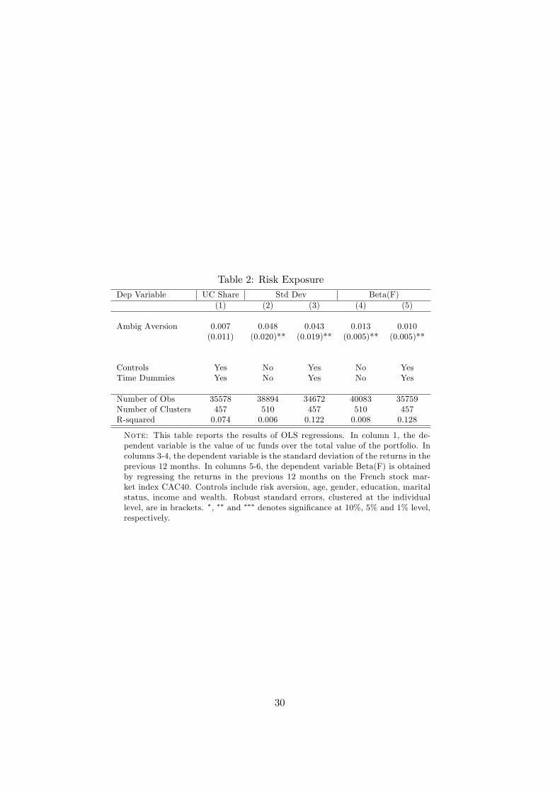
Table 2: Risk ExposureDep Variable UC Share Std Dev Beta(F)

(1) (2) (3) (4) (5)

Ambig Aversion 0.007 0.048 0.043 0.013 0.010(0.011) (0.020)** (0.019)** (0.005)** (0.005)**

Controls Yes No Yes No YesTime Dummies Yes No Yes No Yes

Number of Obs 35578 38894 34672 40083 35759Number of Clusters 457 510 457 510 457R-squared 0.074 0.006 0.122 0.008 0.128

Note: This table reports the results of OLS regressions. In column 1, the de-pendent variable is the value of uc funds over the total value of the portfolio. Incolumns 3-4, the dependent variable is the standard deviation of the returns in theprevious 12 months. In columns 5-6, the dependent variable Beta(F) is obtainedby regressing the returns in the previous 12 months on the French stock mar-ket index CAC40. Controls include risk aversion, age, gender, education, maritalstatus, income and wealth. Robust standard errors, clustered at the individuallevel, are in brackets. ∗, ∗∗ and ∗∗∗ denotes significance at 10%, 5% and 1% level,respectively.

30

Table 3: Under-DiversificationDep Variable Beta(W) Beta(F)-Beta(W) Residuals(1) Residuals(5) R-squared

(1) (2) (3) (4) (5) (6)

Ambig Aversion 0.001 0.009 0.007 0.001 0.001 -0.013(0.003) (0.003)*** (0.002)*** (0.0001)*** (0.0003)*** (0.006)**

Beta(F)+Beta(W) 0.202(0.024)***

Controls Yes Yes Yes Yes Yes YesTime Dummies Yes Yes Yes No No No

Number of Obs 35578 35578 35578 452 452 451Number of Clusters 457 457 457 452 452 451R-squared 0.106 0.061 0.165 0.081 0.073 0.088

Note: This table reports the results of OLS regressions. In column 1, the dependent variable Beta(W)is obtained by regressing the returns in the previous 12 months on the world stock market indexMSCI. In columns 2-3, the dependent is the difference between Beta(F) and Beta(W). In column3, Beta(F)+Beta(W) is the sum of Beta(F) and Beta(W). In column 4, the dependent variable isthe sum of squared residuals in the regression of each client’s returns on the returns in the domesticstock market CAC40 (see equation (2)). In column 5, the dependent variable is the sum of squaredresiduals in the regression of each client’s returns on Fama-French market factors (see equation (3)).In column 6, the dependent variable is the R-squared of the same regression. Controls include riskaversion, age, gender, education, marital status, income and wealth. Robust standard errors, clusteredat the individual level, are in brackets. ∗, ∗∗ and ∗∗∗ denotes significance at 10%, 5% and 1% level,respectively.

31

’

Table 4: Portfolio ReturnsDep Variable Monthly Returns (in %)

(1) (2) (3) (4) (5) (6)

Ambig Aversion 0.016 0.014 0.014 0.013 0.012 0.012(0.006)*** (0.006)** (0.006)** (0.006)** (0.006)** (0.006)**

UC Share 0.056(0.031)*

Std Dev 0.035 0.08(0.014)** (0.039)**

Beta(France) 0.056 -0.189(0.042) (0.148)

Skewness 0.037(0.014)***

Coskewness 0.038(0.021)*

Controls No Yes Yes Yes Yes YesTime Dummies No Yes Yes Yes Yes Yes


Note: This table reports the results of OLS regressions. The dependent variable is the monthlyreturns of the portfolio in percentage points. UC Share is the value of the uc funds over thetotal value of the portfolio. Std Dev and Skewness are respectively the standard deviationand the skewness of the returns in the previous 12 months. Beta(F) is obtained by regressingthe returns in the previous 12 months on the French stock market index CAC40. Coskewnessmeasures the coskewness between the returns and the French stock market index CAC40 inthe previous 12 months. Controls include risk aversion, age, gender, education, marital status,income and wealth. Robust standard errors, clustered at the individual level, are in brackets.∗, ∗∗ and ∗∗∗ denotes significance at 10%, 5% and 1% level, respectively.

32

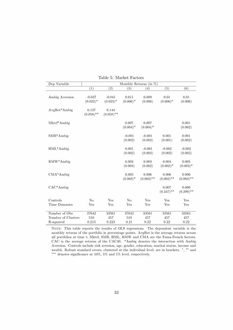
Table 5: Market FactorsDep Variable Monthly Returns (in %)

(1) (2) (3) (4) (5) (6)

Ambig Aversion -0.037 -0.041 0.011 0.009 0.01 0.01(0.022)* (0.023)* (0.006)* (0.006) (0.006)* (0.006)

AvgRet*Ambig 0.137 0.144(0.058)** (0.058)**

Mktrf*Ambig 0.007 0.007 0.001(0.004)* (0.004)* (0.002)

SMB*Ambig -0.001 -0.001 0.001 0.001(0.002) (0.002) (0.001) (0.002)

HML*Ambig 0.001 -0.001 -0.002 -0.002(0.002) (0.002) (0.002) (0.002)

RMW*Ambig 0.003 0.003 0.004 0.005(0.003) (0.002) (0.002)* (0.003)*

CMA*Ambig 0.005 0.006 0.006 0.006(0.003)* (0.003)** (0.002)** (0.003)**

CAC*Ambig 0.007 0.006(0.347)** (0.299)**

Controls No Yes No Yes Yes YesTime Dummies Yes Yes Yes Yes Yes Yes


Note: This table reports the results of OLS regressions. The dependent variable is themonthly returns of the portfolio in percentage points. AvgRet is the average returns acrossall portfolios at time t; Mktrf, SMB, HML, RMW and CMA are the Fama-French factors;CAC is the average returns of the CAC40. *Ambig denotes the interaction with AmbigAversion. Controls include risk aversion, age, gender, education, marital status, income andwealth. Robust standard errors, clustered at the individual level, are in brackets. ∗, ∗∗ and∗∗∗ denotes significance at 10%, 5% and 1% level, respectively.

33

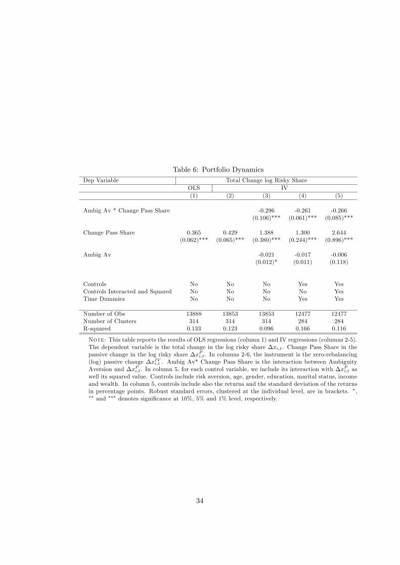
Table 6: Portfolio DynamicsDep Variable Total Change log Risky Share

OLS IV(1) (2) (3) (4) (5)

Ambig Av * Change Pass Share -0.296 -0.261 -0.266(0.106)*** (0.061)*** (0.085)***

Change Pass Share 0.365 0.429 1.388 1.300 2.644(0.062)*** (0.065)*** (0.380)*** (0.244)*** (0.896)***

Ambig Av -0.021 -0.017 -0.006(0.012)* (0.011) (0.118)

Controls No No No Yes YesControls Interacted and Squared No No No No YesTime Dummies No No No Yes Yes


Note: This table reports the results of OLS regressions (column 1) and IV regressions (columns 2-5).The dependent variable is the total change in the log risky share ∆xi,t. Change Pass Share in thepassive change in the log risky share ∆xPi,t. In columns 2-6, the instrument is the zero-rebalancing(log) passive change ∆xIVi,t . Ambig Av* Change Pass Share is the interaction between AmbiguityAversion and ∆xPi,t. In column 5, for each control variable, we include its interaction with ∆xPi,t aswell its squared value. Controls include risk aversion, age, gender, education, marital status, incomeand wealth. In column 5, controls include also the returns and the standard deviation of the returnsin percentage points. Robust standard errors, clustered at the individual level, are in brackets. ∗,∗∗ and ∗∗∗ denotes significance at 10%, 5% and 1% level, respectively.

34

Table 7: Portfolio RebalancingDep Variable Active Change

(1) (2) (3) (4) (5)

Ambig Av * Pass Change -0.050 -0.048 -0.046 -0.044(0.028)* (0.022)** (0.020)** (0.021)**

Passive Change -0.635 -0.472 -0.498 -0.49 -0.518(0.025)*** (0.103)*** (0.081)*** (0.077)*** (0.079)***

Ambig Av 0.001 0.001 0.001 0.001(0.002) (0.002) (0.002) (0.003)

Lagged Risky Share 0.043 0.064(0.009)*** (0.014)***

Controls No No Yes Yes YesTime Dummies No No Yes Yes Yes


Note: This table reports the results of OLS regressions. The dependent variable is theactive change in the risky share and Passive Change is the passive change in the risky share,as defined in equation (5). Ambig Av * Pass Change is the interaction between AmbiguityAversion and Passive Change. Lagged risky share is the risky share in the previous month.Controls include risk aversion, age, gender, education, marital status, income and wealth.Robust standard errors, clustered at the individual level, are in brackets. ∗, ∗∗ and ∗∗∗

denotes significance at 10%, 5% and 1% level, respectively.

35

ambiguity preferences and portfolio choices: … preferences and portfolio choices: evidence from...

Documents