ambikairajah part a: signal processing professor e...
TRANSCRIPT

Part A: Signal Processing
Profes
sor E
. Ambik
airaja
h
UNSW, A
ustra
lia
Chapter 4: Analogue Filter Design
4.1 Butterworth Filters4.2 Design of Low-pass Butterworth Filters4.3 Low-pass to High-pass transformation4.4 Low-pass to Band-pass Transformation4.5 Chebyshev Filters
Profes
sor E
. Ambik
airaja
h
UNSW, A
ustra
lia

4.0 Analogue Filter DesignA very important approach to the design of digital filters is to apply a transformation to an existing analogue filter,
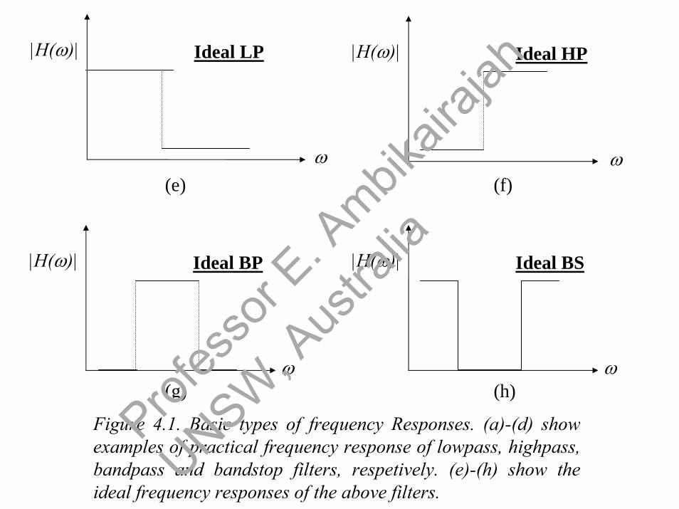
The commonly required types of frequency filter fall into four main groups:
Low-pass (LP)High-pass (HP)Band-pass (BP)Band-stop (BS)Prof
esso
r E. A
mbikair
ajah
UNSW, A
ustra
lia

The frequency responses of these filters are shown in
Figure 4.1 (a to d). Also shown are the frequency responses for the ideal LP, HP, BP and BS filters.
|H(ω)|
ω
LPHP
ω
BP
ω
BS
ω
|H(ω)|
|H(ω)| |H(ω)|
(a) (b)
(c) (d)
Profes
sor E
. Ambik
airaja
h
UNSW, A
ustra
lia
ω
|H(ω)| Ideal LP |H(ω)| Ideal HP
ω
|H(ω)| Ideal BP
ω
|H(ω)| Ideal BS
(e) (f)
(g) (h)
ω
Figure 4.1. Basic types of frequency Responses. (a)-(d) show examples of practical frequency response of lowpass, highpass, bandpass and bandstop filters, respetively. (e)-(h) show the ideal frequency responses of the above filters.
Profes
sor E
. Ambik
airaja
h
UNSW, A
ustra
lia
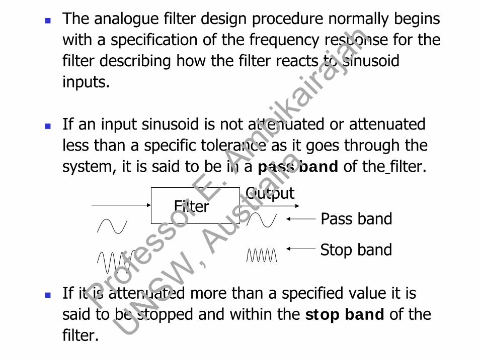
The analogue filter design procedure normally begins with a specification of the frequency response for the filter describing how the filter reacts to sinusoid inputs.
If an input sinusoid is not attenuated or attenuated less than a specific tolerance as it goes through the system, it is said to be in a pass band of the filter.
If it is attenuated more than a specified value it is said to be stopped and within the stop band of the filter.
Output
Pass band
Stop band
Filter
Profes
sor E
. Ambik
airaja
h
UNSW, A
ustra
lia
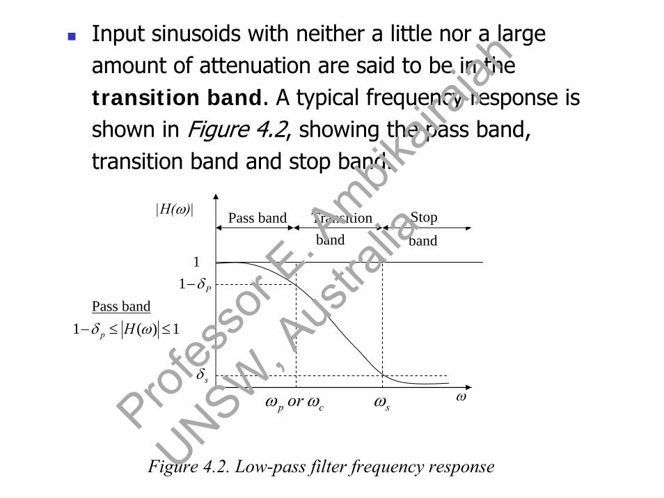
Input sinusoids with neither a little nor a large amount of attenuation are said to be in the transition band. A typical frequency response is shown in Figure 4.2, showing the pass band, transition band and stop band.
|H(ω)|
bandPass band Transition
band1
Stop
ω
Pass band
Figure 4.2. Low-pass filter frequency response
cp orωω sωsδ
1)(1 ≤≤− ωδ Hp
Pδ−1
Profes
sor E
. Ambik
airaja
h
UNSW, A
ustra
lia

The filter with this type of frequency response is called a low-pass filter as it passes all frequencies less than a certain value (or ), called the cut-off frequency and attenuates or stops all frequencies past , the stop band frequency.
The analogue low pass filters are commonly used as anti-aliasing filters that are applied to continuous-time signals before A/D conversion and also used as reconstruction filters.
Profes
sor E
. Ambik
airaja
h
UNSW, A
ustra
lia

Note: The technique used to design analogue filters is to specify a prototype low-pass filter function which is normalized to provide a Cut-off frequency ( ) at 1 rad/sec and then apply transformations to achieve the actual desired cut-off frequencies and filter type.
cω
Profes
sor E
. Ambik
airaja
h
UNSW, A
ustra
lia

Therefore, prime consideration will be given to low-pass filter design using the following design procedures:
Butterworth Low-pass filter- Maximally flat in passband.
ωωpωc
|H(ω)|
1
Profes
sor E
. Ambik
airaja
h
UNSW, A
ustra
lia

Chebyshev I low-pass filter- Maximal ripple in passband.
Chebychev II low-pass filters- Maximal ripple in stopband
|H(ω)|
1
ωωpωc
Profes
sor E
. Ambik
airaja
h
UNSW, A
ustra
lia

Elliptic low pass filter- Minimal transition width- Ripple in both pass band and stopband
Bessel filter- Maximally constant group delay.
Transition band
Pass Band Stop band
ωc
|H(ω)|
1
ωωp
Profes
sor E
. Ambik
airaja
h
UNSW, A
ustra
lia

The ideal, brick-wall, low pass filter prototype is one, which has a unit amplitude frequency response from dc to 1 rad/sec with response dropping to zero there after.
This may be defined in term of the following squared magnitude transfer function:
1
1‘brick wall’ filterIdeal low pass filter
( ) 2ωH
ω
( ) ( ) (4.1) )(1
1)( 22
ωωωω
FjHjHjH
+==−⋅
Where (4.2) 1
100)( 2
⎩⎨⎧
>∞<<
=ωω
ωF
Profes
sor E
. Ambik
airaja
h
UNSW, A
ustra
lia

Since is a polynomial in , must satisfy the lower condition in (4.2). It is not practically feasible to form a polynomial of this type (∞ order).
Therefore approximations to are made. The approximation for due to Butterworth is given by . This yields the following squared magnitude transfer functions:
)( 2ωF 2ω n
nLimF 22 )( ωω
∞→=
)( 2ωF)( 2ωF
nF 22 )( ωω =
(4.3) 1
1)( 22
njHω
ω+
=
(4.4) 1
1)(2n
jHω
ω+
=
(4.2) 1
100)( 2
⎩⎨⎧
>∞<<
=ωω
ωF
Where n is a positive integer.
Profes
sor E
. Ambik
airaja
h
UNSW, A
ustra
lia

4.2 Design of LowpassButterworth Filters [9]
A Butterworth filter of order ‘n’ is defined by
(4.3)equation see (4.5) 21
1)( 2
njH
c⎟⎟⎠
⎞⎜⎜⎝
⎛+
=
ωω
ω
- Cut-off frequency of the filter.cω
Profes
sor E
. Ambik
airaja
h
UNSW, A
ustra
lia

The following properties are easily determined:
1. for all n.
2. for all n; this implies
and
3. is monotonically decreasing function of
ω (i.e. throughout pass band and stop band.)
4. As n gets larger approaches an ideal low-pass frequency response.
1)( 2
0=
=ωωjH
21)( 2 =
= cjH
ωωω 707.0
21)( ==ωjH
dB0.3|)(|log20 −== cjH ωωω
2)( ωjH
2)( ωjH
Profes
sor E
. Ambik
airaja
h
UNSW, A
ustra
lia

5. is called maximally flat at the origin since all order derivatives exist with respect to ωand are zero at the origin.
2)( ωjH
( )( )[ ] ( )[ ]
( ) ( ) ( )⎪⎪⎩
⎪⎪⎨
⎧
+−+−=
+=+
=−
Lnnn
n
n
ccc
c
c
jH
61654
832
21
2
2
1
11
1 21
21
ωω
ωω
ωω
ωω
ωω
ω
Note:
Power series expansion
Profes
sor E
. Ambik
airaja
h
UNSW, A
ustra
lia

2)( ωjH
21
1
ωcω
∞=n
100=n
2=n
1=n
Figure 4.3. The magnitude frequency response of a Butterworth filter
Profes
sor E
. Ambik
airaja
h
UNSW, A
ustra
lia
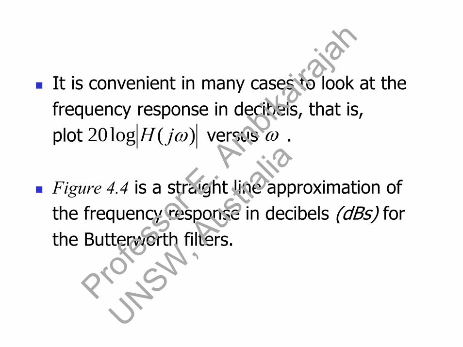
It is convenient in many cases to look at the frequency response in decibels, that is, plot versus .
Figure 4.4 is a straight line approximation of the frequency response in decibels (dBs) for the Butterworth filters.
)(log20 ωjH ω
Profes
sor E
. Ambik
airaja
h
UNSW, A
ustra
lia

n=1 Slope= -20dB/decade
n=2 Slope= -40dB/decade
ω0.1ωc
=20log|H (jω)|
Actual values for n=3
-60dB
-40
-20
-3dB
dB
0
n=3 Slope= -60dB/decade
ωc 100ωc
Figure 4.4. Filter gain plot for analogue Butterworth filters of various orders of n.Prof
esso
r E. A
mbikair
ajah
UNSW, A
ustra
lia
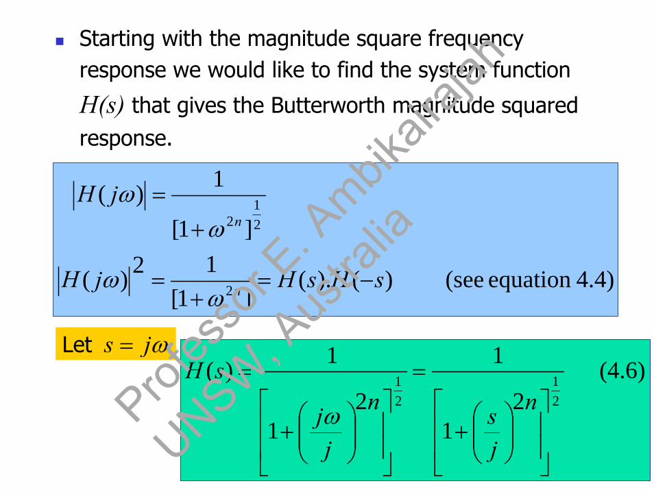
Starting with the magnitude square frequency response we would like to find the system function
H(s) that gives the Butterworth magnitude squared response.
4.4)equation (see )().(]1[
12)(
]1[
1)(
2
21
2
sHsHjH
jH
n
n
−=+
=
+=
ωω
ωω
(4.6) 2
1
1
21
1)(21
21
⎥⎥
⎦
⎤
⎢⎢
⎣
⎡⎟⎟⎠
⎞⎜⎜⎝
⎛+
=
⎥⎥
⎦
⎤
⎢⎢
⎣
⎡⎟⎟⎠
⎞⎜⎜⎝
⎛+
=n
jsn
jj
sH
ω
Let ωjs =
Profes
sor E
. Ambik
airaja
h
UNSW, A
ustra
lia

(4.7) 1
1)(2ns
sH+
=
(4.8) 1
1)(2ns
sH−
=
For n even
For n odd
(4.6) 2
1
1
21
1)(21
21
⎥⎥
⎦
⎤
⎢⎢
⎣
⎡⎟⎟⎠
⎞⎜⎜⎝
⎛+
=
⎥⎥
⎦
⎤
⎢⎢
⎣
⎡⎟⎟⎠
⎞⎜⎜⎝
⎛+
=n
jsn
jj
sH
ω
Profes
sor E
. Ambik
airaja
h
UNSW, A
ustra
lia

)2
(n
j
esπ+
=∴ n -even
642,....,, 1284
=↑=↑=↑
=⎟⎠⎞
⎜⎝⎛±⎟
⎠⎞
⎜⎝⎛±⎟
⎠⎞
⎜⎝⎛±
nnneees
jjj πππ
From equation (4.7) the roots of the denominator, i.e. poles are given by
πjnn ess ±=−=⇒=+ 10)1( 221
2
Profes
sor E
. Ambik
airaja
h
UNSW, A
ustra
lia

From equation (4.8), the roots of the denominator i.e. poles are given by
( ) π2221
2 101 jnn ess ±==⇒=−
nj
nj
eesππ
±±==∴ 2
2
n is odd
,......,, 53πjπjπj eees
±±±=∴
ππ sincos j±3
sin3
cos ππ j±
n = 1 n = 3 n = 5
= -1Profes
sor E
. Ambik
airaja
h
UNSW, A
ustra
lia

The poles of the Butterworth filter all lie in the left-hand side of the s-plane with a locus which is a circle of unit radius whose centre is the s-plane origin.
A plot of the poles the Butterworth function for n = 3(odd) is shown in Figure 4.5.
600
600- 600
- 600H(s)
jω
H(-s)
σ
-1
1 s-plane
Figure 4.5. The s-plane of a butterworth filter with n = 3.
623 =⇒= nn poles of H(s) H(-s)Profes
sor E
. Ambik
airaja
h
UNSW, A
ustra
lia

( ) ( ) (4.6)equation see
1
12n
js
sHsH
⎟⎟⎠
⎞⎜⎜⎝
⎛+
=−⋅
A plot of the poles of the Butterworth function for n = 4(even ‘n’) is shown in Figure 4.6.
H(s)
jω
H(-s)
σ
-1
1s-plane
π/4
π/8
- π/4
-π/8
Figure 4.6. The s-plane of a butterworth filter with n = 4.
n = 4 ⇒ 2n = 8 poles of H(s) H(-s)Profes
sor E
. Ambik
airaja
h
UNSW, A
ustra
lia

Example:
Find the transfer function H(s) for the normalized
Butterworth filter of order 2 (n = 2)sec 1rad/c =ω
Since n = 2 ; 4πj
es±
=
21
21
44jπjSinπCos ±=⎟
⎠⎞
⎜⎝⎛±⎟
⎠⎞
⎜⎝⎛
Profes
sor E
. Ambik
airaja
h
UNSW, A
ustra
lia

σ
s1
s2 s4
s3
jω
π/4π/4
π/4
-1/√2
-1 1
Poles of H(s)H(-s) for a normalized Butterworth filter of order 2
⎥⎦
⎤⎢⎣
⎡⎟⎠⎞
⎜⎝⎛ −−
−⎥⎦
⎤⎢⎣
⎡⎟⎠⎞
⎜⎝⎛ +−
−=
−−=
21
21
21
21
1))((
1)(21
jsjs
sssssH
Normalisedimplies ωc= 1
121)(
2 ++=
sssH
Profes
sor E
. Ambik
airaja
h
UNSW, A
ustra
lia

Example: [9]Determine the transfer function of a Butterworth
filter of the low-pass type with order n = 3. Assume
that the 3dB cut-off frequency rad/sec.
For n = 3, the 2n = 6 poles of H(s)H(-s) are located on a circle of unit radius with angular spacing as
shown in Figure 4.6. Hence allocating the lest-half plane poles to H(s), we define
23
21;
23
21;1 321 jsjss −
−=+
−=−=Prof
esso
r E. A
mbikair
ajah
UNSW, A
ustra
lia

The transfer function of a Butterworth filter of order
3 is therefore
( )( )
( )( )
( )1221
111
23
21
23
211
1
23
2
+++=
+++=
⎟⎟⎠
⎞⎜⎜⎝
⎛++⎟⎟
⎠
⎞⎜⎜⎝
⎛−++
=
sss
sss
jsjsssH
Profes
sor E
. Ambik
airaja
h
UNSW, A
ustra
lia

n Butterworth Polynomials1 s+1
2
3
4
5
122 ++ ss
( )( )112 +++ sss
( )( )184776.1176536.0 22 ++++ ssss
( )( )( )16180.116180.01 22 +++++ sssssProfes
sor E
. Ambik
airaja
h
UNSW, A
ustra
lia

Example: Design of low-pass Butterworth filters [9]
Design an analogue Butterworth filter that has -2dBor better cut-off frequency of 20 rad/sec and at least
10dB of attenuation at 30 rad/sec
k2= -10dB
0k1= -2dB
ωωsωx
|H(ω)|
20 rad/sec
dB =20log|H(jω)| or 10log|H(jω)|2
Profes
sor E
. Ambik
airaja
h
UNSW, A
ustra
lia

(4.3))equation (see
1
1)( 22
n
c
jH
⎟⎟⎠
⎞⎜⎜⎝
⎛+
=
ωω
ω
filter order
⎟⎟⎟⎟⎟
⎠
⎞
⎜⎜⎜⎜⎜
⎝
⎛
⎟⎟⎠
⎞⎜⎜⎝
⎛+
= n
c
jH 22
1
1log10)(log10
ωω
ω
equal to k1 at equal to k2 at
xω
sω
Profes
sor E
. Ambik
airaja
h
UNSW, A
ustra
lia

(4.9)
1
1log10 21
⎟⎟⎟⎟⎟
⎠
⎞
⎜⎜⎜⎜⎜
⎝
⎛
⎟⎟⎠
⎞⎜⎜⎝
⎛+
= n
c
x
k
ωω
(4.10)
1
1log10 22
⎟⎟⎟⎟⎟
⎠
⎞
⎜⎜⎜⎜⎜
⎝
⎛
⎟⎟⎠
⎞⎜⎜⎝
⎛+
= n
c
s
k
ωω
⎟⎟
⎠
⎞
⎜⎜
⎝
⎛⎟⎟⎠
⎞⎜⎜⎝
⎛+=−=>
⎥⎥⎦
⎤
⎢⎢⎣
⎡⎟⎟⎠
⎞⎜⎜⎝
⎛+−=
n
c
n
n
c
x kk2
1
2
1 1log10
1log1log10 ω
ωωω
10
21
101kn
c
x−
=⎟⎟⎠
⎞⎜⎜⎝
⎛+
ωω
(4.11) 110 10
21
−=⎟⎟⎠
⎞⎜⎜⎝
⎛ −kn
c
x
ωω
(4.12) 110 10
22
−=⎟⎟⎠
⎞⎜⎜⎝
⎛ −kn
c
ssimilarlyωω
Profes
sor E
. Ambik
airaja
h
UNSW, A
ustra
lia

From equations (4.11) and (4.12)∴
110
110
10
10
2
2
2
1
−
−=
⎟⎟⎠
⎞⎜⎜⎝
⎛
⎟⎟⎠
⎞⎜⎜⎝
⎛
−
−
k
k
n
c
s
n
c
x
ωω
ωω
110
110
10
102
2
1
−
−=⎟⎟
⎠
⎞⎜⎜⎝
⎛−
−
k
kn
s
x
ωω
⎟⎟⎟
⎠
⎞
⎜⎜⎜
⎝
⎛
−
−=⎟⎟
⎠
⎞⎜⎜⎝
⎛−
−
110
110loglog10
10
10
2
10 2
1
k
kn
s
x
ωω
⎟⎟⎟
⎠
⎞
⎜⎜⎜
⎝
⎛
−
−=⎟⎟
⎠
⎞⎜⎜⎝
⎛−
−
110
110loglog210
10
1010 2
1
k
k
s
xnωωProf
esso
r E. A
mbikair
ajah
UNSW, A
ustra
lia

(4.13) log2
110
110log
10
10
10
10 2
1
⎟⎟⎠
⎞⎜⎜⎝
⎛
⎟⎟⎟
⎠
⎞
⎜⎜⎜
⎝
⎛
−
−
=
−
−
s
x
k
k
n
ωω
If n is an integer we use that value, otherwise we use the next larger integer.
⎟⎠⎞
⎜⎝⎛
⎟⎟⎟
⎠
⎞
⎜⎜⎜
⎝
⎛
−
−
=
−−
−−
3020log2
110
110log
10
10)10(
10)2(
10
n
43709.3 ==n 4th order filter
∴
Profes
sor E
. Ambik
airaja
h
UNSW, A
ustra
lia

From equation (4.9), we have
⎟⎟⎟⎟⎟⎟
⎠
⎞
⎜⎜⎜⎜⎜⎜
⎝
⎛
⎟⎟⎠
⎞⎜⎜⎝
⎛+
=n
c
x
ωω
k2101
1
1log10
sec/3868.21
110
20
11042
1
10)2(2
1
101
rad
nk
xc
=
⎟⎟⎠
⎞⎜⎜⎝
⎛−
=
⎟⎟⎠
⎞⎜⎜⎝
⎛−
=×−−−
ωω∴
Profes
sor E
. Ambik
airaja
h
UNSW, A
ustra
lia

The normalized low-pass Butterworth filter for n = 4can be found from the table given previously
)1( =cω
( )( )184776.1176536.01)( 22 ++++
=ssss
sH
De-normalized transfer function∴
⎟⎟
⎠
⎞
⎜⎜
⎝
⎛+⎟⎟
⎠
⎞⎜⎜⎝
⎛+⎟⎟
⎠
⎞⎜⎜⎝
⎛⎟⎟
⎠
⎞
⎜⎜
⎝
⎛+⎟⎟
⎠
⎞⎜⎜⎝
⎛+⎟⎟
⎠
⎞⎜⎜⎝
⎛=
184776.1176536.0
1)(22
cccc
sssssH
ωωωω
21.3868
( ) ( )394.4575176.39394.4573886.1610209210.0)( 22
6
++++×
=ssss
sH Profes
sor E
. Ambik
airaja
h
UNSW, A
ustra
lia

Example:
Design an analogue Butterworth filter (the filter is monotonic in the pass and stop bands (i.e. no ripples)) which meets the following specifications:
Low-pass filter: 0 to 10 kHz (pass band)
Transition band: 10 to 20 kHzStop band attenuation: -10dB (starts at 20 kHz)
Profes
sor E
. Ambik
airaja
h
UNSW, A
ustra
lia

10 kHz
-10dB
0
ω20 kHz
dB
n
c
jH 22
1
1)(
⎟⎟⎠
⎞⎜⎜⎝
⎛+
=
ωω
ωdbjHat p 10)(log10 ; 2
10 −== ωωω
n
c
p
jH 2102
10
1
1log10)(log10
⎟⎟⎠
⎞⎜⎜⎝
⎛+
=
ωω
ωProfes
sor E
. Ambik
airaja
h
UNSW, A
ustra
lia

( ) 9291022029
1011log1
1log1010
1log101log1010
222
22
10
2
10
2
1010
==⎟⎠⎞
⎜⎝⎛
××
=⎟⎟⎠
⎞⎜⎜⎝
⎛
=⎟⎟⎠
⎞⎜⎜⎝
⎛+⇒
⎟⎟
⎠
⎞
⎜⎜
⎝
⎛⎟⎟⎠
⎞⎜⎜⎝
⎛+=
⎟⎟
⎠
⎞
⎜⎜
⎝
⎛⎟⎟⎠
⎞⎜⎜⎝
⎛+−=−
⎟⎟
⎠
⎞
⎜⎜
⎝
⎛⎟⎟⎠
⎞⎜⎜⎝
⎛+−=−
nnn
c
p
n
c
pn
c
p
n
c
p
n
c
p
ππ
ωω
ωω
ωω
ωω
ωω
5849.12log2
9log
10
10 ==n∴Profes
sor E
. Ambik
airaja
h
UNSW, A
ustra
lia

121)(
2 ++=
sssH
( )22
2
2
)(2
12
1)(
cc
c
cc
ss
sseddenormalissH
ωωω
ωω
++=
+⎟⎟⎠
⎞⎜⎜⎝
⎛+⎟⎟
⎠
⎞⎜⎜⎝
⎛=
Thus we choose n = 2 (even)
Normalized
Profes
sor E
. Ambik
airaja
h
UNSW, A
ustra
lia

4.3 Lowpass to High pass transformation [9]
To transform analogue low-pass filter H(s)with unity cut-off frequency to low-pass filter
H(s) with cut-off frequency , we substitute
cω
cωss →
Profes
sor E
. Ambik
airaja
h
UNSW, A
ustra
lia

Example:
First order Butterworth prototype filter is given by
11)(+
=s
sH Normalized
,5=cω
cωs
55
1
1)(+
=+
=+
=sωs
ω
ωs
sHc
c
c
To transform to new cut-off frequency
we replace s with
Profes
sor E
. Ambik
airaja
h
UNSW, A
ustra
lia

Note: To transform an analogue low-pass
filter H(s) with unit cut-off frequency to high-
pass filter H(s) with cut-off frequency , we substitute
ss cω→
Profes
sor E
. Ambik
airaja
h
UNSW, A
ustra
lia

Example:First order Butterworth prototype filter is given by
To transfer to a high-pass filter with cut-off frequency
We replace ;
11)(+
=s
sH Normalized
;2=cω
ss cω→ 21
1)(+
=+
=s
s
s
sHcω
Note: High-pass filter contains zeros as well as poles
Profes
sor E
. Ambik
airaja
h
UNSW, A
ustra
lia

Example:
3rd order Butterworth filter.)1)(1(1)( 2 +++
=sss
sH
Determine the transfer function of the corresponding high-pass filter with cut off frequency (normalized)1=cω
ssei
ss c 1.. →→ ω
( ) ( )1111111
1)( 2
3
2 +++=
⎟⎟⎠
⎞⎜⎜⎝
⎛++⎟
⎠⎞
⎜⎝⎛
⎟⎠⎞
⎜⎝⎛ +
=sss
s
sss
sH
normalized
Profes
sor E
. Ambik
airaja
h
UNSW, A
ustra
lia

4.4 Low-pass to Band-pass Transformations [9]
By definition, a band pass filter rejects both low and high frequency components and passes a certain band of frequencies some where between them. Thus the frequency response , of a band-pass filter has the following properties.
1. at both 2. for a frequency band centred on ,
where is the mid frequency of the filter
)( ωjH
∞== ωω &00)( =ωjH1)( =ωjH 0ω
0ω
Profes
sor E
. Ambik
airaja
h
UNSW, A
ustra
lia

ωL ω0 ωu
dB = 20log|H(jω)|
ω
Lower cut-off frequency Upper cut-off frequency
1
k1
k2
LuB ωω −=
Bandwidth of the band-pass filter
Profes
sor E
. Ambik
airaja
h
UNSW, A
ustra
lia

To convert unity cut off low-pass filter H(s) into a
Band-Pass filter H(s) with lower cut-off frequency
ωL and the upper cut-off frequency ωu , we replace
Similarly to convert unity cut-off lowpass filter H(s)into a bandstop filter H(s) with lower cutoff
frequency ωL and upper cut-off frequency ωu, we
replace:
)(
2
Lu
uL
sss
ωωωω
−+
→
uL
Lu
sss
ωωωω
+−
→ 2
)(Profes
sor E
. Ambik
airaja
h
UNSW, A
ustra
lia

dB
0
k1
k2
ωL ω1 ω2 ωuω
Band stop filter
Profes
sor E
. Ambik
airaja
h
UNSW, A
ustra
lia

Note (second method): A lowpass to bandpass transformation can be performed by
Bsss o
22 ω+→
)( Lu ωω −
0ω
B - Bandwidth of the band-pass filter
- centre frequency.
Profes
sor E
. Ambik
airaja
h
UNSW, A
ustra
lia

ss cω→
( )Lu
Lu
sss
ωωωω
+−
→ 2ωc/ωp ωc ω
k1
k2
dB
k1
k2
ωL ω1 ω0 ω2 ωu ω
dB
ω1 ωL ω0 ωu ω2
k1
k2
ω0-ωL
≠ ωu-ω0
ω
dB
0k1
k2
1 ωp ω
dB = 20log|H(jω)|
unity cut-offωp.ωc
k1
0
ωc
Butterworth Prototype response Transformed filter response
dB
ω
k2
c
ssω
→
( )Lu
Lu
sss
ωωωω
−+
→2
Summary: Analogue to Analogue Transformation
Profes
sor E
. Ambik
airaja
h
UNSW, A
ustra
lia

Example:The specification for a Butterworth low-pass continuous filter reads as follows:
Cutoff frequency, and Amplitude response to be at least 20dB down
when 3=ω
75.0=cω
ωsωc ω
-20dB
dB
0
Profes
sor E
. Ambik
airaja
h
UNSW, A
ustra
lia

( )
( )
( )⎥⎥⎦
⎤
⎢⎢⎣
⎡⎟⎟⎠
⎞⎜⎜⎝
⎛+−=
⎥⎥⎥⎥⎥
⎦
⎤
⎢⎢⎢⎢⎢
⎣
⎡
⎟⎟⎠
⎞⎜⎜⎝
⎛+
=
⎟⎟⎠
⎞⎜⎜⎝
⎛+
=
n
c
n
c
n
c
jH
jH
jH
22
10
2102
10
22
1log101log10log10
1
1log10log10
1
1
ωωω
ωω
ω
ωω
ω
-20dB at 3=ω
Profes
sor E
. Ambik
airaja
h
UNSW, A
ustra
lia

[ ]nn
210
2
10 )4(1log275.031log1020 +=⇒
⎥⎥⎦
⎤
⎢⎢⎣
⎡⎟⎠⎞
⎜⎝⎛+−=−∴
( )
657.14log2
99log99log4log2;994100)4(1
10
10
1022
==
==⇒=+
∴n
nnn
n = 2 would satisfy the requirement.∴
Profes
sor E
. Ambik
airaja
h
UNSW, A
ustra
lia

Example:
Design an analogue band-pass filter with the following characteristics
-3.0103 dB upper and lower cut-off frequency of 50Hz and 20kHza stop-band attenuation of at least 20dB at 20Hz and 45 kHza monotonic frequency response.
Profes
sor E
. Ambik
airaja
h
UNSW, A
ustra
lia
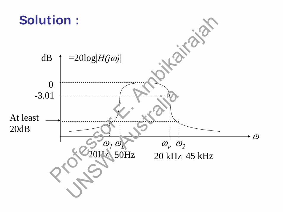
Solution :
20 kHz
At least 20dB
-3.010
ω1 ωL ωu ω2
dB =20log|H(jω)|
ω
20Hz 50Hz 45 kHz
Profes
sor E
. Ambik
airaja
h
UNSW, A
ustra
lia

The monotonic requirement can be satisfied with a Butterworth filter.
sec/1025663.1)1020(2
sec/159.314)50(2sec/1082743.2)1045(2
sec/663.125)20(2
53
532
1
rad
radrad
rad
u
L
×=×=
==×=×=
==
πω
πωπω
πω
BPLP →
( )Lu
uL
sss
ωωωω
−+
→2
Transformation is
Profes
sor E
. Ambik
airaja
h
UNSW, A
ustra
lia

For band-pass filter to satisfy the stop-band attenuation requirement at we must have equality within the transformation. i.e.
Similarly solving ,to satisfy stop-band attenuation requirement at
1ω
( )Lu
uLr j
jjωωωωωωω
−+
=)()(
1
21
( ) 5053.21
21 =
−−
=Lu
uLr ωωω
ωωωω Substitute values for ul ωωω ,,1
rω2ω
( )( )Lu
uLr j
jjωωωωωωω
−+
=2
22Prof
esso
r E. A
mbikair
ajah
UNSW, A
ustra
lia

( ) 2545.22
22 =
−−
=Lu
uLr ωωω
ωωωω
rω
{ }2545.2,5053.2min=rω
Obtained are not equal.
rω
Lu ωω & to obtain BP filter.
First design a low-pass filter H(s) with
and then apply transformation (LP to BP) using
We choose
Profes
sor E
. Ambik
airaja
h
UNSW, A
ustra
lia

The low-pass filter order n can be calculated as before
⎟⎠⎞
⎜⎝⎛
⎟⎟⎟
⎠
⎞
⎜⎜⎜
⎝
⎛
−
−
=
+
+
2545.21log2
110
110log
10
1020
100103.3
10
n
1221)( 23 +++
=∴sss
sH LP
( ) )1025349.1(1094784.3
5
722
××+
=−
+→
ss
sss
Lu
uL
ωωωω
[ ] [ ] 1..........2............2)1025349.1(
1094784.3
1)(2
3
5
73
+++⎥⎦
⎤⎢⎣
⎡××+
=∴s
ssH BP
n = 2.829 and we choose n=3
LP BP
Profes
sor E
. Ambik
airaja
h
UNSW, A
ustra
lia

4.5 Chebyshev Filters [9]
There are two types Chebyshev filters, one containing a ripple in the pass-band (type 1) and the other containing a ripple in the stop-band(type 2).
A type 1 – Low-pass normalized (unit bandwidth) Chebyshev filter with a ripple in the pass-band is characterized by the following magnitude squared frequency response:
[ ]22
2
)(11)(
ωεω
nTjH
+=
Where )(ωnT is the nth order Chebyshev polynomial
Profes
sor E
. Ambik
airaja
h
UNSW, A
ustra
lia

Chebyshev polynomials can be generated and thus defined from the following recursiveformula :
( ) 2 )()(2 21 >−= −− nTTT nnn ωωωω
1)(0 =ωT ( ) ωω =1Twith and
Profes
sor E
. Ambik
airaja
h
UNSW, A
ustra
lia

The list of first 6 Chebyshev polynomials is given in table below:
n Chebyshev Polynomial:
0 11
2
3
4
5
6
ω12 2 −ωωω 34 3 −
188 24 +− ωωωωω 52016 35 +−
1184832 246 −+− ωωω
)(ωnT
Profes
sor E
. Ambik
airaja
h
UNSW, A
ustra
lia

Note: This type of equi-ripple function results from use of Chebyshev cosine polynomials.
( )
( ) 1 for coshcosh)(
1 for coscos)(
1
1
>=
≤=
−
−
ωωω
ωωω
nT
nT
n
n
Profes
sor E
. Ambik
airaja
h
UNSW, A
ustra
lia

[ ]252
25 )(1
1|)(|ωε
ωT
jH+
=
211ε+
(a)
(b)1
10.58778
0.3124
T5(ω)
1
-11 ω-1
ω
For n = 5
Profes
sor E
. Ambik
airaja
h
UNSW, A
ustra
lia

It is noticed that for n = 5, the Chebyshevpolynomial oscillates between +1 and -1 while outside the interval it grows towards .
(See Figure (a) )
This same type of oscillation takes place for every Chebyshev polynomial and causes the equal magnitude ripple in the as shown in
Figure (b).
Profes
sor E
. Ambik
airaja
h
UNSW, A
ustra
lia

The amplitude of oscillates between 1 and
as ω goes from -1 to +1, but the
period of oscillations are not equal .
The heads to zero outside -1 and 1, because the magnitude of the chebyshev
polynomial leads toward ∞ as ω goes away from -1 or +1
211ε+
2)( ωjH
Profes
sor E
. Ambik
airaja
h
UNSW, A
ustra
lia

( )ωεω 22
2
11)(
nTjH
+=
even is when11
1)0(1
1)( 2222
0n
TjH
n
=+
=+
== εε
ωω
( ) odd isn where0=ωnT
Profes
sor E
. Ambik
airaja
h
UNSW, A
ustra
lia

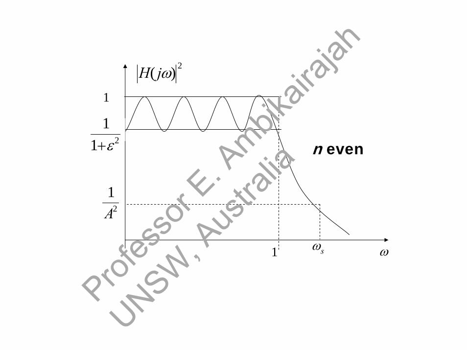
Note :The magnitude squared frequency response
oscillates between 1 and within the pass-band,
the so called equiripple, and has a value of at , the cut-off frequency.
2)( ωjH
211ε+
211ε+
1=cω
ω1 ωs
1
211ε+
2
1A
2)( ωjH
n odd
Profes
sor E
. Ambik
airaja
h
UNSW, A
ustra
lia
2)( ωjH
2
1A
ω1 ωs
1
n even21
1ε+
Profes
sor E
. Ambik
airaja
h
UNSW, A
ustra
lia

is monotonic outside the pass-band , including both transition band and the stop-band.
2)( ωjH
( )[ ]22
2
11)(
ωεω
nTjH
+=
( )[ ] 1 22 >>ωεω nTincreasesas
[ ] ( )ωεω
ωεω
nn TjH
TjH 1)(
)(1)( 22
2 =⇒=∴
⎟⎟⎠
⎞⎜⎜⎝
⎛+=
)(1log20)(log20ωε
ωnT
jH
Profes
sor E
. Ambik
airaja
h
UNSW, A
ustra
lia

[ ])(log20log20)(log20)(log20
1010
1010
ωεωεω
n
n
TTjH+−=
−=
nnhighabove for see table ωω 12 ; −
ωεωεω
101010
101
101010
log202log20)1(log20log202log20log20)(log20
nnjH nn
+−+=
++=− −
Therefore the attenuation
( ) ωεω 101010 log20)1(6log20||log20 nnjH +−+≈− Profes
sor E
. Ambik
airaja
h
UNSW, A
ustra
lia

Clearly the Chebyshev approximation depends on the values of є and n.
The maximum permissible ripple fixes the value of є, and once this value of є has been determined the value of the attenuation in the stop-band fixes the value of the filter complexity n.
Profes
sor E
. Ambik
airaja
h
UNSW, A
ustra
lia

Example:
A Chebyshev low-pass characteristic is required to
have a maximum pass-band ripple of 1.2dB and an
attenuation of at least 25dB at ω = 2.5. Determine
the values of є and n.
[ ]22
2
)(11)(
ωεω
nTjH
+=
1)(Tn =ωAt ω = 1, the ripple is 1.2dB and
Profes
sor E
. Ambik
airaja
h
UNSW, A
ustra
lia

5641.0110
101101
1
11log10dB2.1
102.1
2
102.1
2102.1
2
210
=⇒−=
=+⇒=+
⎟⎠⎞
⎜⎝⎛+
=−
−
εε
εε
ε
At ω = 2.5, namely in the stop-band, attenuation = -25dB.
25 = 20log10 є+ 6 (n-1) + 20n log10 ω25 = 20log10(0.5641) + (n-1)6 + 20*n log102.5n = 2.577 and we choose n = 3.
∴
Profes
sor E
. Ambik
airaja
h
UNSW, A
ustra
lia

|H(jω)|ripple amplitude
α1
ω
( )21
21
1
ε+21
11ε
α+
−=
)(11)(2 ωε
ωnT
jH+
=
1)0(T ; 1
1)( n20=
+=
= εω
ωjH
129.05641.01
11 =+
−=α
ripple amplitude
Profes
sor E
. Ambik
airaja
h
UNSW, A
ustra
lia

Having obtained є and n we could continue to derive H(s)
)(11)( 22
2
ωεω
nTjH
+=
01 22 =⎟⎟⎠
⎞⎜⎜⎝
⎛+
jsTnε
It can be shown that H(s) can be obtained by finding the roots of
It can be shown that the poles of fall on an
ellipse as shown below.
⎟⎟⎠
⎞⎜⎜⎝
⎛+
jsTn
221 ε
Profes
sor E
. Ambik
airaja
h
UNSW, A
ustra
lia

Poles of Hn(-s)Poles of Hn(s)jω
σ
ellipse
Poles on axis for odd n
Profes
sor E
. Ambik
airaja
h
UNSW, A
ustra
lia

Example : n = 6 & є = 0.7647831
jω
σ
0.90.70.26
-0.17
Profes
sor E
. Ambik
airaja
h
UNSW, A
ustra
lia

Note:It can be shown that a comparison of the normalized Chebshev pole locations with the normalized Butterworth pole locations reveals that the imaginary parts are identical and the real part of the Butterworth pole times a factor “tanh(Ak)” is equal to the real part of the Chebyshev pole
Hence knowing the normalized Butterworth poles the corresponding normalized Chebyshev poles can be derived.
The denormalized Chebyshev poles are obtained by multiplying the normalized Chebshev poles by a denormalising–factor equal to cosh(Ak).
)1(sinh1 1
ε−=
nAwhere k
Profes
sor E
. Ambik
airaja
h
UNSW, A
ustra
lia

H(s) can be calculated for the previous example as follows:
for n = 3 , the Butterworth poles are ( selecting in the left-hand of the s-plane)
4457.05641.01sinh
31 1 =⎟
⎠⎞
⎜⎝⎛= −
KA
4184.0tanh =kA1009.1cosh =kA
866.05.03
4sin3
4cos
01sincos
866.05.03
2sin3
2cos
3
2
1
jjp
jjp
jjp
−−=+=
+−=+=
+−=+=
ππππ
ππ
Profes
sor E
. Ambik
airaja
h
UNSW, A
ustra
lia

Multiplying the real parts of p1, p2 and p3 by
tanh(Ak) we obtain the normalized Chebyshev poles.
Multiplying by cosh(Ak), we obtain the de-normalized Chebyshev poles
866.02092.0
04184.0
866.02092.0
'3
'2
'1
jp
jp
jp
−−=
+−=
+−=
'3
'2
'1 ,, ppp
9534.02303.0
04606.0
9534.02303.0
"3
"2
"1
jp
jp
jp
−−=
+−=
+−=
Profes
sor E
. Ambik
airaja
h
UNSW, A
ustra
lia

)9534.02303.0)(9534.02303.0)(4606.0()(
jsjssksH
++−++=∴
1)9534.02303.0)(9534.02303.0)(46060.0(0)( =
+−== jj
ksH ω
gain DC 4431.0=∴k
De-normalized Chebyshev transfer function
Profes
sor E
. Ambik
airaja
h
UNSW, A
ustra
lia

Obtain values for є and n
Obtain normalized Butterworth Poles
Select only the poles in the LHS of the s-plane
Obtain corresponding normalized Chebyshev
poles
Obtain denormilisedChebyshev ploes
obtain value of k
H(s)
Multiply real parts of the poles by tanh Ak
Multiply the poles (real & imaginary) by cosh Ak
)1(sinh1 1
ε−=
nAk
Recommended design process for deriving H(s) for a Chebyshev low-pass filter [9]
Profes
sor E
. Ambik
airaja
h
UNSW, A
ustra
lia