Louisiana State UniversityLSU Digital Commons

LSU Doctoral Dissertations Graduate School

2015

Ambit of Multiphase CFD in Modelling TransportProcesses Related to Oil Spill Scenario andMicrofluidicsAbhijit RaoLouisiana State University and Agricultural and Mechanical College, arao4@lsu.edu

Follow this and additional works at: https://digitalcommons.lsu.edu/gradschool_dissertations

Part of the Chemical Engineering Commons

This Dissertation is brought to you for free and open access by the Graduate School at LSU Digital Commons. It has been accepted for inclusion inLSU Doctoral Dissertations by an authorized graduate school editor of LSU Digital Commons. For more information, please contactgradetd@lsu.edu.

Recommended CitationRao, Abhijit, "Ambit of Multiphase CFD in Modelling Transport Processes Related to Oil Spill Scenario and Microfluidics" (2015).LSU Doctoral Dissertations. 1121.https://digitalcommons.lsu.edu/gradschool_dissertations/1121

AMBIT OF MULTIPHASE CFD IN MODELLING TRANSPORT PROCESSES RELATED TO OIL SPILL SCENARIO AND MICROFLUIDICS

A Dissertation

Submitted to the Graduate Faculty of the Louisiana State University and

Agricultural and mechanical College in partial fulfillment of the

requirements for the degree of Doctor of Philosophy

in

Cain Department of Chemical Engineering

by

Abhijit Rao B.E in Chemical Engineering, Visveswaraiah Technological University,2007

M.S in Chemical Engineering, Louisiana State University, 2014 December 2015

ii

This work is dedicated to my parents, friends and family members…

iii

Acknowledgements

I would like to express my sincere gratitude to my advisor, Professor Krishnaswamy Nandakumar for

supporting my present study and research, for his patience, motivation and enthusiasm. I cherish the opportunity

to be part of enlightening discussions with him on various topics during the course of this work. His guidance has

thoroughly helped me during the course of this research and writing of this dissertation. I could not have imagined

of having a better mentor for this study. I would also like to thank Prof. Kalliat T Valsaraj and Prof. Louis

Thibodeaux for the encouragement, and insightful comments. I wish my gratitude to Dr. Francisco Hung and Dr.

Brooks Ellwood for being part of dissertation committee.

My sincere thanks to Dr. Rupesh Reddy, Dr. Mayur Sathe, Dr. Mranal Jain, Dr. Chuliang Wu and Dr. Zhuyi

Yu who have helped me with my research work in a great way. Special thanks to Dr. Dandina Rao, for allowing me

to use the IFT apparatus in his lab. I would also like acknowledge Dr. Franz Ehrehenseur, who helped me with

designing the experiments in the initial stages. I thank my fellow members of EPIC (Enabling Process

Intensification through Computation) research group: Dr. Yuehao Li, Dr. Shivkumar Bale, Oladapo Ayeni,

Guongqiang He, Chenguang Zhang , Aaron Harrington, Mutharasu, Jielin, Daniel, Zhizhong for the stimulating

discussions, which were amazingly fruitful. I also appreciate help extended by Agnimitro and Getnet with

OpenFOAM. I appreciate the help provided by Allan Huang in processing the images from experiment. Last but

not the least, I would like to thank my parents, family members and friends who have been a constant source of

inspiration and have supported me throughout my life.

I would also take this opportunity to acknowledge High Performance Computing (HPC), at LSU, Louisiana

Optical Network Initiative (LONI) and XSEDE for providing access to the computational resources. This work was

made possible by grant received from CMEDS consortium under Gulf of Mexico Research Initiative.

iv

Contents

Acknowledgements .........................................................................................................................................iii

Abstract……... ............................................................................................................................................................... vii

Chapter 1 Introduction ................................................................................................................................ 1 1.1 What is Multiphase CFD? .................................................................................................................................... 1 1.2 Scope and Organization of dissertation .............................................................................................................. 3 1.3 References ........................................................................................................................................................... 5

Chapter 2 Deep water oil spill and Modelling ................................................................................................. 6 2.1 Numerical model development for capturing Large Scale dynamics .................................................................. 8 2.2 Scales involved in model development ............................................................................................................. 11 2.3 References ......................................................................................................................................................... 13

Chapter 3 Dynamics of a crude oil droplet in a surfactant laden water column ............................................... 15 3.1 Introduction ...................................................................................................................................................... 15 3.2 Physical background and overview ................................................................................................................... 16 3.3 Experimental Setup and methodology .............................................................................................................. 20 3.4 Droplet formation at low rates ......................................................................................................................... 22 3.5 Dimensionless numbers .................................................................................................................................... 24 3.6 Interfacial tension Measurement ...................................................................................................................... 24

3.6.1 Axisymmetric Drop Shape Analysis (ADSA) ................................................................................................ 26 3.6.2 Dynamic and Equilibrium IFT ..................................................................................................................... 27 3.6.3 Interfacial tension Measurement in Ambient Cell ..................................................................................... 28 3.6.4 Diffusion controlled adsorption model ...................................................................................................... 31

3.7 Mathematical Model ......................................................................................................................................... 32 3.7.1 Governing Equations .................................................................................................................................. 33 3.7.2 Interface tracking in VOF method .............................................................................................................. 34 3.7.3 Geometric reconstruction scheme ............................................................................................................ 34 3.7.4 Numerical methods and simulation setup ................................................................................................. 35

3.8 Observations and Discussion ............................................................................................................................. 37 3.8.1 Experiment ................................................................................................................................................. 37 3.8.2 Numerical Results ...................................................................................................................................... 44

3.9 Conclusions ....................................................................................................................................................... 51 3.10 Nomenclature ................................................................................................................................................. 52 3.11 References ....................................................................................................................................................... 53

Chapter 4 Influence of unsteady Mass transfer on Droplet Dynamics ............................................................ 56 4.1 Overview ........................................................................................................................................................... 58 4.2 Experiment ........................................................................................................................................................ 62 4.3 Numerical Model ............................................................................................................................................... 65

4.3.1 Governing Equations .................................................................................................................................. 66 4.3.2 Implementation of mass transfer in ANSYS Fluent® .................................................................................. 67 4.3.3 Numerical methods and simulation setup ................................................................................................. 69 4.3.4 Estimation of mass transfer coefficient ..................................................................................................... 71

4.4 Importance of combined transfer over forced convection at low Re ............................................................... 75 4.5. Results .............................................................................................................................................................. 76

4.5.1 Experimental .............................................................................................................................................. 76 4.5.2 Numerical Results ...................................................................................................................................... 77 4.5.3 Effect on dynamics of droplet .................................................................................................................... 79

v

4.5.4 Pressure distribution around the droplet during different stages of motion ............................................ 81 4.5.5 Flow separation around the droplet .......................................................................................................... 82

4.6 Effect of surfactant on the mass transfer .......................................................................................................... 83 4.7 Conclusions ....................................................................................................................................................... 84 4.8 Nomenclature.................................................................................................................................................... 85 4.9 References ......................................................................................................................................................... 86

Chapter 5 Jet dynamics in the Laminar Regime ............................................................................................ 89 5.1 Jet breakup dynamics ........................................................................................................................................ 89 5.2 Jet breakup regimes .......................................................................................................................................... 90 5.3 Results from the numerical Investigation ......................................................................................................... 91

5.3.1 Jet break up in kerosene – water system................................................................................................... 92 5.3.2 Effect of surfactant addition on the jet breakup ....................................................................................... 92 5.3.3 Effect of mass transfer on the jet break up ............................................................................................... 95

5.4 Nomenclature.................................................................................................................................................... 96 5.5 References ......................................................................................................................................................... 97

Chapter 6 Integration of CFD with Population Balance approach for prediction of size distribution of droplets in submerged turbulent multiphase jets .......................................................................................... 99

6.1 Introduction ...................................................................................................................................................... 99 6.2 Effect of turbulence on droplet dynamics ....................................................................................................... 100 6.3 Turbulent jet dynamics .................................................................................................................................... 101 6.4 Numerical modelling ....................................................................................................................................... 105

6.4.1 Multiphase Models .................................................................................................................................. 105 6.4.2 Turbulence Models .................................................................................................................................. 109 6.4.3 Population Balance Models ..................................................................................................................... 111

6.5 Model Integration ........................................................................................................................................... 116 6.6 Model Validation ............................................................................................................................................. 119

6.6.1 Computational domain and Boundary conditions ................................................................................... 120 6.7 Mixture model v/s Eulerian Two Fluid Model ................................................................................................ 124 6.8 Results and discussion ..................................................................................................................................... 126

6.8.1 Effect of dispersed phase flow rates on droplet size distribution ........................................................... 126 6.8.2 Effect of dispersant concentration on droplet size distribution .............................................................. 127 6.8.3 Effect of presence of gas phase on DSD................................................................................................... 129

6.9 Conclusion ....................................................................................................................................................... 132 6.10 Nomenclature ............................................................................................................................................... 132 6.11 References ..................................................................................................................................................... 133

Chapter 7 Implementation of Continuous Species Transport Model to capture solute transfer across fluid interfaces ................................................................................................................................ 137

7.1 Basics of ‘interFoam’ solver............................................................................................................................. 137 7.2 Continuous Species Transport Model ............................................................................................................. 141 7.3 Model development in OpenFOAM® .............................................................................................................. 142 7.4 Case setup in OpenFOAM® ............................................................................................................................. 145 7.5 Nomenclature.................................................................................................................................................. 146 7.6 References ....................................................................................................................................................... 146

Chapter 8 Mass transfer from a slug traversing in a Microchannel ............................................................... 148 8.1 Introduction .................................................................................................................................................... 148 8.2 Regimes during the slug flow in microchannel ............................................................................................... 150 8.3 Mass transfer process from slug ..................................................................................................................... 152 8.4 Numerical Model ............................................................................................................................................. 154 8.5 Evolution of concentration profiles in dispersed and continuous phase ........................................................ 157

vi

8.6 Effect of Flow rates ratio on the slug parameters ........................................................................................... 161 8.7 Mass transfer during slug formation in squeezing and dripping regimes ....................................................... 164 8.8 Effect of varying Q on the Mass transfer in channel in squeezing and dripping regimes ............................... 165 8.9 Conclusions ..................................................................................................................................................... 173 8.10 Nomenclature ............................................................................................................................................... 174 8.11 References ..................................................................................................................................................... 175

Chapter 9 Conclusions and Outlook .......................................................................................................... 177 9.1 Summary and key contributions ..................................................................................................................... 177 9.2 Future work ..................................................................................................................................................... 178

Appendix A File organization in cstFoam solver ........................................................................................... 180

Appendix B Problem Setup for cstFoam solver ........................................................................................... 195

Appendix C Choice of boundary conditions for slug flow in microchannels ................................................... 211

Appendix D Permissions ............................................................................................................................. 216

Vita……………. ...................................................................................................... ……………………………………………….223

vii

Abstract

During the ‘Deepwater Horizon’ accident in the deep sea in 2010, about 4.9 million barrels of oil was

released into the Gulf of Mexico, making the spill one of the worst ocean spills in recent times. To mitigate the ill

effects of the event on the environment, subsea injection of dispersants was carried out. Dispersant addition

lowers the interfacial tension at oil/water interface and presence of local turbulence enhances the droplet

disintegration process. The oil droplets contain a plethora of hydrocarbons which are soluble in water. In deep

spill scenarios, droplets spend large amounts of time in water column; hence, the dissolution process of soluble

hydrocarbons becomes important. In this study, our focus is to exploit the capabilities of multiphase CFD in

developing an integrated numerical model which accounts for various transport processes and hence would

effectively guide us in predicting the fate of oil mass. In the initial stages, studies were conducted to understand

these transport processes at a very fundamental level where the effect of surfactant, on the dynamics of crude oil,

droplet rising in a stagnant column, was investigated. To capture the subsurface dissolution of hydrocarbons from

oil droplet, a unique experiment was devised wherein a binary organic mixture, representing a pseudo oil droplet

comprising of volatile and non-volatile hydrocarbons, was employed to study the effect of unsteady mass

transport on the overall dynamics of the droplet. In the next phase of project, we developed a numerical model, by

integrating traditional multiphase CFD models and turbulence models, with a population balance (PB) approach,

for predicting the droplet size distribution resulting from the interaction of turbulent oil jets with the surrounding

quiescent environment.

Apart from the simulations specific to oil spill related situations, the multiphase CFD was also employed to

study the fluid flow in micro-channels. The mass transfer mechanisms in micro-channels for immiscible fluids in

squeezing and dripping regimes were studied by employing the numerical model, which couples the features of

the traditional Volume of fluid method and the Continuous Species transport approach for evaluating the

concentration fields inside dispersed and continuous phase.

1

Chapter 1 Introduction

1.1 What is Multiphase CFD?

Multiphase Computational Fluid Dynamics is branch of CFD which deals with systems with more than one

phase. Phase is primarily defined by the thermodynamic state that the matter belongs to (gas/liquid/solid). The

carrier fluid is one which is present in system in a larger proportion and is normally termed as continuous phase.

The phase which is present in a smaller quantity is known as dispersed phase. The multiphase CFD modelling is

science of capturing the interactions between different phases in a system and translating the effect of these

interactions on overall dynamics of the fluids flowing in the system by using numerical means. Phasic volume

fractions, denoted by α, are commonly used by CFD codes to distinguish between different phases in a system. A

multiphase flow finds its importance in many flow situations which are relevant to industry. Depending on the

interactions among different phases involved multiphase flows can be categorized as;

1. Gas-liquid flows (distillation, absorption)

2. Liquid –Liquid flows (Extraction)

3. Gas - solid flows (Fluidization, pneumatic transport)

4. Liquid – solid flows (Slurry flow, Sedimentation)

5. Three phase flows (involves solid/liquid/gas ;for example, hydrotransport of oil sands)

The classification of multiphase flows is normally expressed in terms of flow pattern and flow regime. A

flow pattern is essentially a visual representation of different phases in a system. It gives a gross idea of overall

phase distributions and hence indicates the extent of global separation among the phases present in a system ;

the two extremes being a fully dispersed flow pattern’ where the dispersed phase is distributed as

droplets/bubbles / particles in a continuous phase , and ‘separated flow pattern’ where two or more phases exist

as parallel streams. A flow regime, on the other hand, indicates the influence of these flow structures on the

physical nature of the system. Apart from laminar and turbulent flow regimes, depending on the fluid –fluid

combination, flow rates , flow orientation and flow confinement ; multiphase system can also exhibit stratified

flow, bubbly flow, slug flow , plug flow, annular flow etc. Some of the above described flows have been in

illustrated in Figure 1.1.

2

Figure 1.1 Flow regimes in multiphase systems; L-L: liquid liquid, G-L: Gas liquid, L-S: Liquid solid and G-S: Gas solid.

During modelling multiphase systems, the first process would be to identify the regime of the flow.

Different approaches are available for solving multiphase problems using Computational Fluid dynamics.

1. Euler Lagrange approach

2. Euler Euler approach

3. Fully resolved approach

In Euler Lagrange approach, the fluid phase is treated as a continuum and flow fields are evaluated by

solving Navier Stokes equation. The dispersed phase is composed of discrete particles whose motion is tracked by

solving particle motion equation based on the overall force balance around the particle. It should be noted that the

dispersed phase is allowed to exchange mass, momentum and energy with the continuous phase. For flow

situations where the presence of discrete particles does not drastically influence local continuous flow fields, the

evaluation of discrete phase trajectories are based on fixed continuous phase flow field (one way coupling).

However, the influence of dispersed phase on the continuous phase flow field can be accounted for by adopting

two phase coupling where both discrete and continuous phase equation with mass, energy and momentum

exchange terms are solved alternately. The Euler Lagrange approach is reasonable when the volume fraction of

discrete phase is low. Models such as Discrete Particle Models (DPM) and Discrete Element models (DEM) fall

under this category.

L-L or G-L L-L /G-L/L-S/G-S L-L or G-L L-S

L-S G-S

3

The Euler-Euler approach treats different phases in the system as interpenetrating continua. Phasic

volume fractions , a continuous function in time and space, are employed to differentiate between various

phases present in the system. Mixture model approach and Euleraian- Eulerian / Two fluid Model (TFM) approach

are two most widely used methods. In mixture model, single set of momentum and continuity equations are

solved along with equation for volume fraction function. The relative velocities between the phases are calculated

using traditional methodologies like drift flux[1]

. Two fluid model offers a more rigorous approach in the sense that

momentum and continuity equations are solved for each phase. The influence of one phase on others is captured

by including momentum exchange terms. Closure models are required for evaluation of body forces appearing in

the momentum equation. For the situations where appropriate closure models are available, the flow fields

evaluated by TFM bear greater accuracy. However, it comes at an expense of greater computational requirements.

Euler- Euler approach can be used for simulating bubble columns, fluidized beds, cyclone separators etc. More

details on these models have been provided in the later chapters.

Fully resolved approach solves the Navier Stokes Equation without using closure models for any of its

terms. Many Direct Numerical Simulations (DNS) for multiphase system exist in literature [2-4]

. Under this

framework, many methods such as Volume of Fluid (VOF), Level Set etc. are available for simulating liquid –liquid

flows. In this work, the applicability of VOF approach for different flow situations has been demonstrated. VOF is

essentially used for tracking interface between immiscible fluids, by solving volume fraction equation along with

momentum and continuity equations shared by the phases. VOF approach can be employed for simulating

stratified flows, free surface flows, disintegration of jets etc.

1.2 Scope and Organization of dissertation

In this work, we demonstrate the raw power of multiphase CFD models in capturing the various transport

processes associated with deepwater oil spill scenarios. Further, we show the applicability of the developed

multiphase models in simulating flow in microchannels. The models described in this work have been developed

using commercially available CFD code ANSYS® Fluent and an open source package OpenFOAM®.

The organization of this dissertation is as follows. The first part of the thesis shows the model

development for capturing phenomena relevant to oil spill scenario occurring at different scales. The next chapter

introduces the various aspects of deepwater oil spill and strategy adopted towards development of a

4

comprehensive integrated model. During Deepwater Horizon incident in 2010, in order to mitigate the ill effects of

oil in marine waters, around 25 percent of total dispersant was injected near the source of blowout. Before

exploring the overall effect of dispersants on large scale dynamics, it is imperative to gain a good understanding of

droplet dynamics at a more fundamental level. In Chapter 3, we describe the effect of presence of surfactant on

the dynamics of droplet rising in the stagnant water column. In deep water oil spills, accounting for dissolution of

hydrocarbons from oil to water phase becomes important. We describe the effect of the unsteady mass transfer

on the dynamics of a single organic droplet ascending in the water column in Chapter 4. The effect of surfactant

and unsteady mass transfer on the jet dynamics in the laminar regime has been covered in Chapter 5. Chapter 6

presents the extension of previously developed models to capture the large scale dynamics, by integration of CFD

with Population Balance Modelling Approach. Chapter 7 discusses the development of an improved mass transfer

model in OpenFOAM platform. The applicability of such models in capturing mass transfer in the slug flow regime

in microchannels, has been demonstrated in Chapter 8. The contributions of this dissertation have been

summarized in Chapter 9. Figure 1.2 summarizes the various scenarios for which the multiphase CFD models were

developed during the course of this study.

Figure 1.2 Multiphase CFD models developed for different scenarios.

(m)

5

1.3 References

[1] T. Hibiki, M. Ishii, One-dimensional drift-flux model and constitutive equations for relative motion between

phases in various two-phase flow regimes, International Journal of Heat and Mass Transfer, 46 (2003) 4935-4948.

[2] Y. Ge, L.-S. Fan, 3-D Direct Numerical Simulation of Gas–Liquid and Gas–Liquid–Solid Flow Systems Using the Level-Set and Immersed-Boundary Methods, in: B.M. Guy (Ed.) Advances in Chemical Engineering, Academic Press, 2006, pp. 1-63.

[3] N. Di Miceli Raimondi, L. Prat, C. Gourdon, P. Cognet, Direct numerical simulations of mass transfer in square microchannels for liquid–liquid slug flow, Chemical Engineering Science, 63 (2008) 5522-5530.

[4] S. Tenneti, R. Garg, C.M. Hrenya, R.O. Fox, S. Subramaniam, Direct numerical simulation of gas–solid suspensions at moderate Reynolds number: Quantifying the coupling between hydrodynamic forces and particle velocity fluctuations, Powder Technology, 203 (2010) 57-69.

6

Chapter 2 Deep water oil spill and Modelling

During the ‘Deepwater Horizon’ accident in the deep sea in 2010, that about 4.9 million barrels[1]

of oil

was released into the Gulf of Mexico, making the spill one of the worst ocean spills in recent times. The oil was

released into the ocean at the depth of 5000 ft. An ocean column essentially represents a stratified environment,

i.e. the density varies (increases) with depth. When the oil is introduced into stagnant environment (ocean water),

by accidental release in huge quantities, the gushing oil loses its momentum energy and results in entrainment of

surrounding water to form a plume. The oil phase initially emerges as jet , however , the entrainment of the

surrounding medium leads to formation of plume. A typical plume is thus a multiphase mixture of oil, gas and

ambient water. The plume consists of a gas core, which serves as a source of buoyancy and allows it to rise in the

water column. As reported by Socolofsky[2]

, the presence of cross currents can cause the plume to bend and lead

to the fractionation of gas phase from the main plume. The shear interaction between the oil / gas plumes and the

ambient fluid results in formation of droplets with wide size distribution[3]

. The above phenomenon is depicted in

the Figure 2.1. Beyond terminal layer, rise of droplets are purely due to buoyancy.

Figure 2.1 Snapshot of ocean water column during oil spill(from Oil in Sea: Inputs, Fates and Effects

[4])

The oil droplets rising through water column can take following pathways;

a) Reach surface if they are large enough, to have significant rise velocities, and coalesce to form surface slicks.

b) The oil on the surface can lose lighter fraction to atmosphere through evaporate and become denser than

surrounding fluid and sink.

c) Get trapped (small droplets) in neutrally buoyant regions, not contributing to surface slicks.

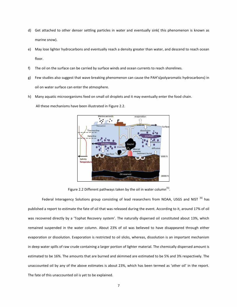
7

d) Get attached to other denser settling particles in water and eventually sink( this phenomenon is known as

marine snow).

e) May lose lighter hydrocarbons and eventually reach a density greater than water, and descend to reach ocean

floor.

f) The oil on the surface can be carried by surface winds and ocean currents to reach shorelines.

g) Few studies also suggest that wave breaking phenomenon can cause the PAH’s(polyaromatic hydrocarbons) in

oil on water surface can enter the atmosphere.

h) Many aquatic microorganisms feed on small oil droplets and it may eventually enter the food chain.

All these mechanisms have been illustrated in Figure 2.2.

Figure 2.2 Different pathways taken by the oil in water column

[5].

Federal Interagency Solutions group consisting of lead researchers from NOAA, USGS and NIST

[6] has

published a report to estimate the fate of oil that was released during the event. According to it, around 17% of oil

was recovered directly by a ‘Tophat Recovery system’. The naturally dispersed oil constituted about 13%, which

remained suspended in the water column. About 23% of oil was believed to have disappeared through either

evaporation or dissolution. Evaporation is restricted to oil slicks, whereas, dissolution is an important mechanism

in deep water spills of raw crude containing a larger portion of lighter material. The chemically dispersed amount is

estimated to be 16%. The amounts that are burned and skimmed are estimated to be 5% and 3% respectively. The

unaccounted oil by any of the above estimates is about 23%, which has been termed as ‘other oil’ in the report.

The fate of this unaccounted oil is yet to be explained.

8

One of the remediation methods that were employed, to mitigate the ill effects of oil that had entered

the water on environment, was done by spraying dispersants. Nearly 2.1 million gallons[7]

of dispersant used during

‘Deepwater Horizon’. About 30% of dispersant was injected at point of release. Due to lowering of interfacial

tension and the existing turbulence the large droplets disintegrate into smaller droplets and disperse in the water

column.

The droplets and gas bubbles rising in the column contain plethora of organic components which diffuse

into the surrounding water under existing concentration gradients. The presence of these alien components in

water has detrimental effect on marine environment. In order to have an estimate amount of these components

entering the water body, it is important to understand the dynamics of droplet, which affects the mass transfer

rates. The presence of surfactants in the system further complicates the system.

From above discussion it is evident that the success of a comprehensive numerical model to predict the

fate of oil droplets during such events would depend on its ability to capture various transport processes

associated with the deep water oil spills. The model should be capable to addressing various aspects such the

lowering of interfacial tensions, effect of turbulence on disintegration of droplets, mass transfer etc.

2.1 Numerical model development for capturing Large Scale dynamics

In the initial stages of project, the objective was to verify the capability of existing multiphase CFD models

in capturing the large scale phenomena. Qualitative simulations were carried using previously described

multiphase models. As it can be seen in Figure 2.3, the model correctly predicts the effect of ambient crosscurrents

on single phase plume. In presence of a stronger crossflow, the oil mass takes longer time to reach the surface.

Figure 2.3 Effects of ambient current on the oil plume.

9

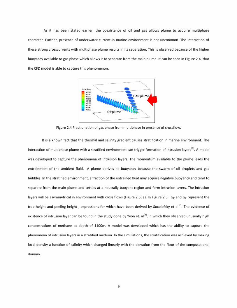
As it has been stated earlier, the coexistence of oil and gas allows plume to acquire multiphase

character. Further, presence of underwater current in marine environment is not uncommon. The interaction of

these strong crosscurrents with multiphase plume results in its separation. This is observed because of the higher

buoyancy available to gas phase which allows it to separate from the main plume. It can be seen in Figure 2.4, that

the CFD model is able to capture this phenomenon.

Figure 2.4 Fractionation of gas phase from multiphase in presence of crossflow.

It is a known fact that the thermal and salinity gradient causes stratification in marine environment. The

interaction of multiphase plume with a stratified environment can trigger formation of intrusion layers[8]

. A model

was developed to capture the phenomena of intrusion layers. The momentum available to the plume leads the

entrainment of the ambient fluid. A plume derives its buoyancy because the swarm of oil droplets and gas

bubbles. In the stratified environment, a fraction of the entrained fluid may acquire negative buoyancy and tend to

separate from the main plume and settles at a neutrally buoyant region and form intrusion layers. The intrusion

layers will be asymmetrical in environment with cross flows (Figure 2.5, a). In Figure 2.5, and represent the

trap height and peeling height , expressions for which have been derived by Socolofsky et al[2]

. The evidence of

existence of intrusion layer can be found in the study done by Yvon et. al[9]

, in which they observed unusually high

concentrations of methane at depth of 1100m. A model was developed which has the ability to capture the

phenomena of intrusion layers in a stratified medium. In the simulations, the stratification was achieved by making

local density a function of salinity which changed linearly with the elevation from the floor of the computational

domain.

10

Figure 2.5 Effect of stratification on plume dynamics and formation of intrusion layers.

Evaposinking is another interesting phenomenon associated with oil spills. The oil at surface may lose

volatile components through evaporation (to air phase) or dissolution (to water phase). With continuous loss of

volatiles the density of oil gradually increases and a stage is reached when it exceeds the density of water and the

oil mass starts to sink in water column. A model in CFD employing traditional Volume of fluid approach is able to

capture this phenomenon. This has been illustrated in Figure 2.6, where the region marked by red represents the

oil phase.

(a)

(b)

Density profile in stratified environment

Image from experiment Contour plot from dye phase

11

Figure 2.6 Different stages during Evaposinking phenomenon.

2.2 Scales involved in model development

As seen in previous sections, all large scale phenomena are guided by fundamental transport processes

like mass transfer, movement of dispersant at oil/water interface etc. An actual oil spill involves millions of

droplets interacting with each other as they rise in the water column. The transport processes further complicates

their dynamics which ultimately influences their fate. So, in the earlier part of the journey towards development of

a comprehensive model, we have sought to gain better understanding of these transport processes at a more

fundamental level.

A snapshot of water column would reveal the existence of different flow regimes as one moves away from

the source of oil leakage to the water surface. The interaction between the oil droplets is more pronounced in the

regions near the blowout. As one gets closer to water surface, oil droplets acquire their individualities before

coalescing to form an oil slick. A more clarity on different scales involved in this event can be understood by

considering the injection of oil phase being into stagnant water column. At a very low flow rates, as the liquid is

introduced droplet forms and detaches at the tip of the nozzle. This constitutes the dripping regime. As the flow

rate is gradually increased, at a critical flow rate, jet emerges from the nozzle and this velocity at which jet

formation takes place is known as jetting velocity denoted by . The droplets are produced from the jet, when

the interfacial instability develops on the surface of jet and causes its breakup. The length of the continuous

filament extending from the tip of the nozzle to the point where jet disintegrates is known as the ‘jet breakup

length’. The jet breakup length increases with increase in nozzle velocity until a critical velocity . The jet in

this regime (between and ) is laminar and the dynamics of jet remain axisymmetric. The droplets are

Air

water

Air

waterwater

Air

(a) (b) (c)

12

formed by disintegration of jet and are mono-dispersed in nature. When the nozzle velocity is increased beyond

the jet loses axisymmetric behavior and breakup length falls. The jet breakup in this regime occurs because of

asymmetrical sinuous disturbances. Unlike in laminar regime, the droplets are ejected laterally from the surface of

jet and are poly-dispersed. When the flow rate exceeds a critical velocity , a regime known as ‘atomization’ is

observed in which the droplets are again found to be produced at nozzle. During this regime a large number of

very fine droplets of non-uniform sizes are formed. The entire process is shown in Figure 2.7. It can be seen that

for ‘dripping regime’ a fully resolved approach like Volume of Fluid can be employed for capturing flow dynamics.

However, when system becomes more chaotic and complicated as it happens during ‘atomization regime’ one has

to content with averaged approaches like Mixture / Eulerian- Eulerian.

Figure 2.7 Modelling strategies for different regimes of jet breakup (images from experiment conducted by

Masatuni et. al[10]

).

Considering the complexity of the problem, the model development was divided into two stages. In the

first stage, different factors affecting the flow dynamics of single droplet in a quiescent system were studied. We

primarily investigated the effect of surfactant (chief component of a dispersant), on the dynamics of crude oil

droplet rising in a stagnant column. The influence of unsteady mass transfer on droplet dynamics was also studied.

The models thus developed were also used to predict the jet dynamics in laminar regime. The details on this can

be found in chapters 3,4 and 5. In the second stage, an attempt was made to develop models for a system which

Dripping AtomizationRej Flow regime

Volume of fluid

Mixture/ Two Fluid Model

Multiphase modelling approach

13

was representative of a real oil spill event. The existence of high turbulence along with presence of dispersants in

the marine environment results in disintegration of droplets. The fate of oil droplets depends on the size of oil

droplets existing in the system. To address this, a more complicated atomization regime was considered and

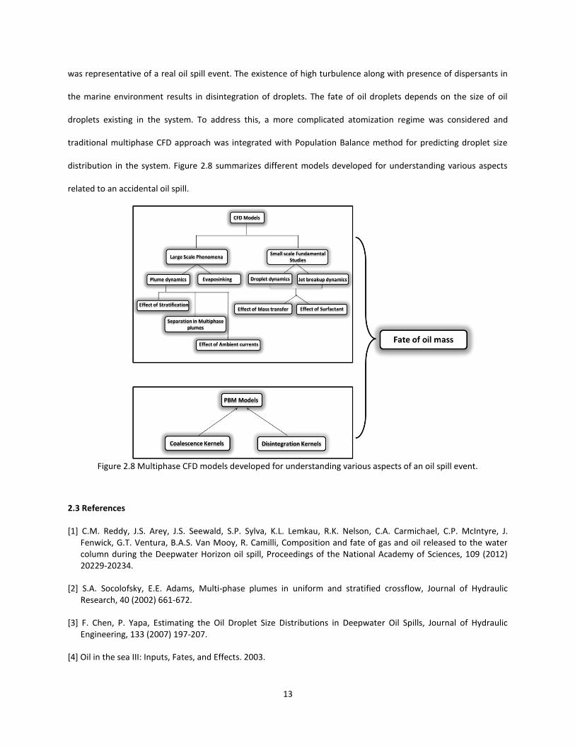
traditional multiphase CFD approach was integrated with Population Balance method for predicting droplet size

distribution in the system. Figure 2.8 summarizes different models developed for understanding various aspects

related to an accidental oil spill.

Figure 2.8 Multiphase CFD models developed for understanding various aspects of an oil spill event.

2.3 References

[1] C.M. Reddy, J.S. Arey, J.S. Seewald, S.P. Sylva, K.L. Lemkau, R.K. Nelson, C.A. Carmichael, C.P. McIntyre, J. Fenwick, G.T. Ventura, B.A.S. Van Mooy, R. Camilli, Composition and fate of gas and oil released to the water column during the Deepwater Horizon oil spill, Proceedings of the National Academy of Sciences, 109 (2012) 20229-20234.

[2] S.A. Socolofsky, E.E. Adams, Multi-phase plumes in uniform and stratified crossflow, Journal of Hydraulic Research, 40 (2002) 661-672.

[3] F. Chen, P. Yapa, Estimating the Oil Droplet Size Distributions in Deepwater Oil Spills, Journal of Hydraulic Engineering, 133 (2007) 197-207.

[4] Oil in the sea III: Inputs, Fates, and Effects. 2003.

14

[5] K.T.V. Louis J. Thibodeaux, Vijay T. John, Kyriakos D. Papadopoulos, Lawrence R. Pratt, and Noshir S. Pesika., , Marine Oil Fate: Knowledge Gaps, Basic Research, and Development Needs; A Perspective Based on the Deepwater Horizon Spill, Environmental Engineering Science, 28(2) (February 2011) 87-93.

[6] B. Lehr, S. Bristol, A. Possolo, Oil Budget Calculator, Deep water Horizon, in, The Federal Interagency Solutions Group, Oil Budget Calculator Science and Engineering Team, 2010.

[7] E.B. Kujawinski, M.C. Kido Soule, D.L. Valentine, A.K. Boysen, K. Longnecker, M.C. Redmond, Fate of Dispersants Associated with the Deepwater Horizon Oil Spill, Environmental Science & Technology, 45 (2011) 1298-1306.

[8] S.A. Socolofsky, E.E. Adams, C.R. Sherwood, Formation dynamics of subsurface hydrocarbon intrusions following the Deepwater Horizon blowout, Geophysical Research Letters, 38 (2011) L09602.

[9] S.A. Yvon-Lewis, L. Hu, J. Kessler, Methane flux to the atmosphere from the Deepwater Horizon oil disaster, Geophysical Research Letters, 38 (2011) L01602.

[10] E.E. Adams , S.M. Masutani Experimental and Analytical Study of Multi-phase Plumes in a Stratified Ocean with Application to Deep Ocean Spills, in, 2002.

15

Chapter 3 Dynamics of a crude oil droplet in a surfactant laden water column*

3.1 Introduction

It has been mentioned in the earlier chapters that the dispersant addition serves as one of the important

remediation methods in the event of oil spill. During Deepwater horizon oil spill incident almost 2.1 million

gallons[1]

of dispersant used during ‘Deepwater Horizon’. For the very first time, subsea injection was tried and

about 30% of total dispersant used towards mitigation, was injected at point of release. The dispersant is

composed of many components. Surfactant is the chief ingredient in the dispersant which acts as a surface

modifying agent and facilitates the lowering of interfacial tension at the oil water interface. The combined effect

of diffusion and convection due to the bulk fluid motion transports the surfactant molecules in the continuous

phase and delivers it to a region (sub-surface) close to oil/water interface. The surfactant molecules move to

interface through the process of adsorption and ultimately reduce the interfacial tension. The lowering of

interfacial tension imparts flexibility to the oil water interface which under local shear stretches itself and

disintegrates into smaller droplets. In the marine environment the disintegration process is enhanced because of

synergistic effect of local turbulence and reduced interfacial tension. Thus, the dispersant addition does not

destroy oil mass, rather it brings about dilution by dispersing oil into fine droplets which are transported to farther

region by underwater currents. In this chapter, we investigate the effect of surfactant dissolved in the continuous

phase on the dynamics of a crude oil droplet rising in a quiescent medium.

Investigation of droplet dynamics in these systems is of paramount importance because it furnishes

essential information on parameters like effective interfacial area, rise velocities etc., which govern the transport

processes occurring in the system and also facilitate determination of the fate of the droplet in the water column.

The presence of dispersant changes the interfacial properties and strongly influences dynamics of the droplets.[2, 3]

The time taken by oil droplets to reach the surface depends chiefly on their size and shape which is affected by the

presence of dispersants. The existing turbulent field enhances the interaction of droplets with each other in the

near field region. However, in far field region the droplets rising in column are not influenced greatly by the

* This chapter previously appeared as, Rao A., Reddy R., Ehrenhauser F., Nandakumar K., Thibodeaux L., Rao D. & Valsaraj K.T., “Effect of surfactant on dynamics of crude oil droplet: Experimental and Numerical Investigation” . Can. J. Chem. Eng. 2014; 92:2098-2114. It is reprinted by permission of John Wiley and Sons.

16

presence of other droplets and succeed in maintaining their individuality. In this work we make an effort to seek a

good understanding pertaining to a single droplet behavior, rising in the water column, in presence or absence of a

surfactant.

3.2 Physical background and overview

The motion of droplet rising in the column of continuous medium is quite different from that of rigid

sphere of same mass and volume. The deformable surface of the drop allows the shear, experienced by the rising

droplet, to influence the motion fluid inside the droplet[4]

. This gives rise to internal circulations inside the droplet

which effectively reduces the drag on the droplet and hence, the droplet always exhibits (in a pure system free of

contaminants) a higher rise velocity than that of a corresponding rigid sphere.

For a spherical droplet, the rise velocity depends on many factors such as the strength of internal

circulations, wake structure behind the droplet etc.[5]

The internal circulation has a strong dependence on the ratio

of viscosities of dispersed fluid to that of continuous fluid, denoted by . Higher the ratio, lesser would be the

tendency for generation of internal circulations. The purity of the system is another factor which controls the

internal circulation development. Presence of impurities like a surfactant on the surface of droplet impedes the

internal circulation and as fluid particles starts behaving more like their rigid counterpart.

Another factor that affects the motion of the droplet is the distortion caused by the external flow to its

shape which essentially speaks of its departure from spherical shape. The shape of droplet is the result of two

competitive forces; the surface tension force, which always tries to restore the spherical shape and the shear and

pressure force, which tries to deform the droplet. The presence of surfactants lowers the interfacial tension at the

interface and allows the interface to stretch more under existing hydrodynamic forces. The viscous droplets

generally assume an ellipsoidal shape at moderate Re[5]

.

The adsorption of surfactant at interface begins as soon as the dispersed phase is injected into the

column. Further, as the droplet starts rising in the water column, more surfactant gets adsorbed on to its surface

and brings in changes to the interfacial tension which influences the dynamics of the droplet. The adsorbed

surfactant is convected by the surface flow to the trailing edge and accumulates. Thus, the existing surface

convection causes the concentration of surfactant to fall at the leading edge of the moving droplet and rise at its

trailing edge. This concentration differential gives rise to a surface tension gradient along the interface and gives

17

rise to Marangoni stresses, which sets up convection from region of lower interfacial tension to higher one and

consequently dampens the internal circulations inside the droplet. Wang et al.[6]

through their numerical study

have shown that presence of surfactant in high concentration is capable of keeping the interface saturated and

this consequently opposes the development of surface tension gradients and allows the revival of internal

circulations in the droplets which might have waned in presence of Marangoni stresses. This however is valid

under the assumption that the surfactant does not impart rigidity at the interface.

The movement of a surfactant molecule from the bulk to the interface can be broken into following steps

(a) diffusive and convective transport of surfactant molecules from bulk phase to region close to oil-water

interphase (subsurface); (b) adsorption of surfactant on the surface of an oil droplet. Depending on the local

surfactant concentration, the interfacial tension at oil water interface is lowered and local shear and turbulence

bring in the droplet disintegration. Once the surfactant molecules are delivered to the subsurface region

adsorption comes in to the picture. The adsorption of the surfactant is presumed to follow Langmuir kinetics.

Once adsorbed, surfactant molecules tend to lower the interfacial tension. The relation between the interfacial

tension and the bulk concentration of surfactant in the continuous phase is given by Szyszkowski equation

- ( ) (3.1)

where is he interfacial tension in absence of the surfactant , m is the maximum concentration of the surfactant

at the surface, C concentration of the surfactant in the continuous phase , corresponds to the number of species

constituting the surfactant and adsorbing at the interface. For SDS[7]

, which is univalent ionic surfactant n 2.

It is intuitive to assume that the interface with low interfacial tension will easily be able to transfer the

momentum from external fluid to the internal fluid and hence has a tendency to induce circulations more easily,

however, it has commonly been observed that the presence of surfactant at the interface actually weakens the

internal circulations.[3]

It is believed that the surface active molecules form a barrier layer and impart some rigidity

to the interface (which depends on the characteristics of a surfactant and its interaction with the interface) and

hence resists the transfer of shear and impede circulation. Further, if the surface active molecule possesses

property to reduce the interfacial tension then under existing shear the one might expect droplet to undergo

significant deformation. Thus, overall reduction in the velocity of the droplet in a surfactant laden environment

18

can be attributed to the enhancement in overall drag force due to synergistic effect of internal circulation strength

and droplet deformation [8]

.

Many studies have been conducted in the past for gaining insight on single droplet dynamics. The work of

Garner et al.[8]

, focused on the role of internal circulations on the droplet dynamics. They conducted experiments

with a mixture of carbon tetrachloride and cyclohexane as dispersed phase and 83% (by weight) solution of

glycerol in water as a continuous phase. Aluminum particles were added in the dispersed phase to visualize the

flow patterns inside the droplet. They also studied the effect of surfactant addition on droplet and concluded that

the presence of surfactant retards the internal circulations in the droplet.

The shape of a small droplet (< 1mm) is spherical because of the internal pressure produced by the

interfacial tension; however, larger droplets become oblate spheroids. The shape acquired by the droplet depends

on the balance between forces which tend to restore spherical shape (surface tension force) and forces which are

disruptive in nature (inertial force). The motion of large droplets through immiscible fluid was experimentally

investigated by Wairegi et al. [9]

for a wide range of Eötvos numbers. They have reported different shapes of

droplets which include ellipsoidal and spherical-caps with and without skirts, crescents, biconcave disks, toroids

and wobbling irregular droplets.

The larger droplets are also known to exhibit significant oscillations. To explore the cause and effect of

oscillations , Winnikow et al. [4]

, studied the motion of droplets in purified systems, and presented results on the

behavior of falling organic droplets covering a wide range of Re from 100 to 1000. In their work, they calculated

drag force for both non-oscillating and oscillating droplets and identified that at the transition point, a sharp

increase was seen in the drag coefficient. In addition they observed that the onset of droplet oscillations was

marked with the periodic shedding of vortices behind the droplet.

In literature[5] the departure of the droplet from spherical is often represented by the term aspect ratio

E, which refers to the ratio between the minor axis to that of the major axis. Thus,

19

Though lot of research work has been done on single droplet dynamics, not many researchers have

studied a system where the presence of surfactant in continuous phase influences the dynamics of droplet with

high viscosity ratio (ratio of dispersed to continuous phase) at intermediate Re. Such systems are important and

have many practical applications .The objective of this study was to study experimentally and computationally the

dynamics of crude oil droplets, released in.to a quiescent pool of water, containing surfactant. The viscosity ratio

was around 25. The droplets of varying sizes were produced by three sets of nozzles whose internal diameter

varied from 1mm to 8mm. The dynamics of droplets were observed to change considerably with increase in the

concentration of the surfactant (Sodium dodecyl sulfate) in the continuous phase, which varied from 0 to 750ppm.

The observable parameters such as aspect ratio E, which is the ratio of maximum vertical dimension to maximum

horizontal dimension within the droplet; and the rise velocity, were measured in the experiment. Most of the

droplets were found to follow an ellipsoidal regime. However, at higher surfactant concentrations, large droplets

exhibited significant wobbling (oscillations about the horizontal axis) and traced a zigzag path.

A numerical model based on finite volume method with an interface reconstruction technique based on

piecewise linear representation for tracking the oil-water interface was developed using the commercial CFD

package ANSYS Fluent®. The surface tension effects were included in model by sticking to Continuum surface

force(CSF) approach suggested by Brackbill[10]

. 2D axisymmetric assumptions were made to perform numerical

simulations for droplets which travelled in rectilinear path with no or very insignificant wobbling. A complete 3D

simulation was required to demonstrate the dynamics of the large droplets.

In present study, it is essential to consider the fact that the Re exhibited by the droplets was in the range

200-900, and droplets at higher surfactant concentration displayed significant wobbling and oscillations. Hence,

under the lack of any experimental evidence it is difficult to state with certainty if surfactant SDS is able to impart a

perfect rigidity along the droplet surface. Further, the viscosity of dispersed phase in this case is greater than that

of continuous phase by almost 25 folds and hence the internal circulations developed inside the droplet can be

expected not to be very strong. And hence one can expect that the influence of the weakening of internal

circulations on overall drag experienced by the droplet will not be significant. In fact, the major contributor

towards the increase in drag could be the distortion experienced by the droplet due to the reduction in the

20

interfacial tension. With these arguments, in current work, we assume that the interface stays mobile and it is

always at its equilibrium IFT (based on the diffusion controlled model described in later sections).

3.3 Experimental Setup and methodology

The experimental setup consisted of a vertical rectangular column made of acrylic glass (PMMA), with

height of 100cm and square base of length 30cm, filled with water. The assembly of all major components has

been shown in Figure 3.1, a. The dispersed phase, crude oil, was released into the stagnant pool of water through

nozzle with the help of a syringe pump. A long PTFE tube was used to connect the syringe mounted on syringe

pump and the nozzle. The crude oil used in the experiments was taken from Bosco Field, LA. In this study, an

anionic, soluble surfactant, Sodium dodecyl sulfate (SDS 95 %) supplied by Sigma Aldrich Inc. was used. The

properties of these materials are listed in Table 3.1.The crude oil was injected in a controlled manner such that

only single droplet was released at a time. Three well machined nozzles of internal diameters ranging from 1mm to

8.5mm were used to produce crude oil droplets with varying diameters. Since the dimensions of the tank were far

greater than the droplet size, the effect of the walls on the dynamics of droplets was minimal. The specifications of

nozzles used have been illustrated in Table 3.2.

The images of droplets were captured using a high speed camera, Canon® EX-ZR200, capable of capturing

multiple images at the shutter speed of 1/1000 second and frame rate of 30fps. The system was illuminated using

60W fluorescent lamps kept at the side corners of the tank. A background sheet was provided to improve the

quality of images. The processing of images was done by subtracting the background and converting it into binary

image by using a threshold feature available in ImageJ®. The densities of the continuous and dispersed phases

were measured using DMA HP density meter and the Ostwald viscometers were used for measuring their

viscosities. A graduated measuring scale was used as a part of the experimental setup and during image

processing the number of pixels for a known distance was determined and this was used for estimating the droplet

size and subsequently for evaluating its velocity. The deviation of droplet from plane of nozzle was cm in X and

Y direction and this resulted in overall error in measurement of the length of less than 3%.

21

Figure 3.1 (a) Schematic representation of experimental setup 1)nozzle 2)syringe pump 3)Illuminating system 4)submersible pump 5) water column 6)camera ; (b) parameters used in the experiment for analyzing droplet

dynamics.

Table 3.1 Physical properties of the materials/reagents used in the experiment

Physical properties @ 250C

Dispersed Phase : Crude Oil

Origin Bosco Field,LA

Density 888.8 kg/m

3

Viscosity 25.25 cP

Continuous Phase : Water(tap)

Density 998 kg/m

3

Viscosity 1cP

Surfactant : Sodium dodecyl sulfate (SDS)

D

C

A

B

(a) (b)

22

Table 3.2 Specifications of the nozzles used in the experiment

Experiments were conducted at different concentrations (viz. 0, 100, 250, 500 and 750ppm) of surfactant

SDS, in the continuous phase. The tank was scrupulously cleaned after each run and the water was replaced

before surfactant concentration in the continuous phase was graduated to a higher level. After the surfactant

addition, the water in tank was kept under circulation with the help of a small submersible pump for an hour. This

was done to ensure a sufficient mixing. The water in the column was allowed to reach a quiescent state, prior to

the introduction of oil droplets into the column. The mass of oil that accumulated on the surface was removed

intermittently. All experiments were conducted at ambient conditions.

The diameter of the oil droplet was estimated from the sequence of images taken near the tip of the

nozzle, at the time when the droplet was about to pinch off from the nozzle (‘A’ in Figure 3.1, b.). The

measurements were done on 20 droplets and average value was calculated. The rise velocity was obtained by

processing high definition video taken from the camera. The average rise velocity was estimated by noting the

time required for 15 droplets to travelling a distance of around 70cm (point ‘B’ to ‘D’ in Figure 3.1, b.); the

referenced origin being located about 10 cm above the release point. The residence time of the droplets in the

tank varied between 10-15 s. The shape change in droplet was expressed in terms of an aspect ratio E (ratio of

minor to major axis), which essentially gave extent of its departure from spherical shape. For aspect ratio

measurement, the images were captured near the upper section of the tank, between ‘C’ and ‘D’ in Figure 3.1, b.

3.4 Droplet formation at low rates

In present work we have focused on the dynamics of single droplet moving in the continuous phase and

hence the droplet formation during dripping regime will be considered. The drop formation depends on the

balance of following forces:

Buoyancy force

A1 A2 A3

ID(mm) 1.0 2.65 8.5

Droplet dia(mm) 3.1-4.7 4.4-6.1 5.5-8.5

Material Borosilicate Borosilicate Steel

23

Interfacial force.

The force due to buoyancy is attributed to the density difference between the dispersed phase and the

continuous phase. The buoyancy force tends to separate the droplet from the nozzle whereas the interfacial force

acts to keep droplet attached to the nozzle. Under static conditions, there exists opposition between buoyancy and

interfacial tension force at the nozzle and the moment the lifting force exceeds the restraining force the droplet

pinches off the nozzle.

The size of the droplet pinching off from the nozzle can approximately be calculated through a simple

balance between the acting forces. The volume of the droplet clinging to the nozzle is given by

( )

where is the nozzle diameter, is the interfacial tension and corresponds to the density difference between

the dispersed and the continuous phase. After pinch off a small volume of droplet is retained by the tip, the actual

volume of the released droplet is slightly lesser than . To account for this Harkins[11]

proposed a factor

which is given by

( )

Mori[12]

proposed a correlation for evaluation of

[

(

)

⁄

]

(

)

⁄

( )

The pinch off mechanism can be categorized into two stages;

Lift off

Necking & Pinch off.

Figure 3.2 shows the stages involved during the droplet formation. The first stage corresponds to the

point when the droplet experiences lift and elongates slightly, once all external forces balance each other. This is

followed by the final phase wherein the droplet gets detached from the main fluid filament after necking.[13, 14]

24

Figure 3.2 Formation of a droplet during experiment and its detachment from the nozzle i) lift off stage ii) necking

stage iii) pinch off stage

3.5 Dimensionless numbers

The shape of a buoyancy driven droplet is influenced by non-dimensional numbers such as Reynolds

Number (Re), Eötvos Number (Eo) and Morton Number (M). The Reynolds number is ratio of inertial forces to

viscous forces. The effects of interfacial tension on the dynamics of droplet are incorporated in Eötvos and Morton

Numbers. The Eötvos number gives a measure of strength of buoyant forces to the interfacial forces, whereas

Morton Numbers signifies the effect of the competing viscous forces and interfacial forces.

In this study, the ranges of above dimensionless quantities were: , and

Figure 3.3 depicts the shape regimes for various droplets studied in the experiment. As

shown clearly, droplets at low M primarily exhibit ellipsoidal shape. However, an increase in M (which indicates a

reduction in interfacial tension forces) causes the droplets to enter a wobbling regime.

3.6 Interfacial tension Measurement

Interface holds a special significance in determining the dynamics of an immiscible droplet. The

characteristic of an interface controls the manner in which the flow organizes itself inside the droplet. To

elaborate, a flexible interface is able to transmit the momentum of the outer fluid to the inner fluid more readily

when compared to a rigid interface. The change in the behavior of an interface drastically affects the processes like

heat and mass transfer occurring around the droplet. Surface tension originates because of the non-uniform forces

25

Figure 3.3 Shape regimes of droplet in the experiment (adapted from Clift et al.[5])

acting on the molecules in the interface. The molecules in the bulk fluid experience equal amount of

intermolecular forces, known as cohesive forces, from the surrounding like molecules. However, the molecules at

the interface are exposed to two different kinds of forces: forces acting on them due to like molecules (cohesive

force) and due to molecules of different species (adhesive force). The molecules at interface are pulled inwards by

the intermolecular forces due like molecules surrounding the lower part of molecule. Thus, to attain a lower

energy state, the interface acts as stretchable layer. The interfacial tension (IFT) at the oil-water interface is

lowered, when the surfactant is adsorbed at the surface of oil droplet.

26

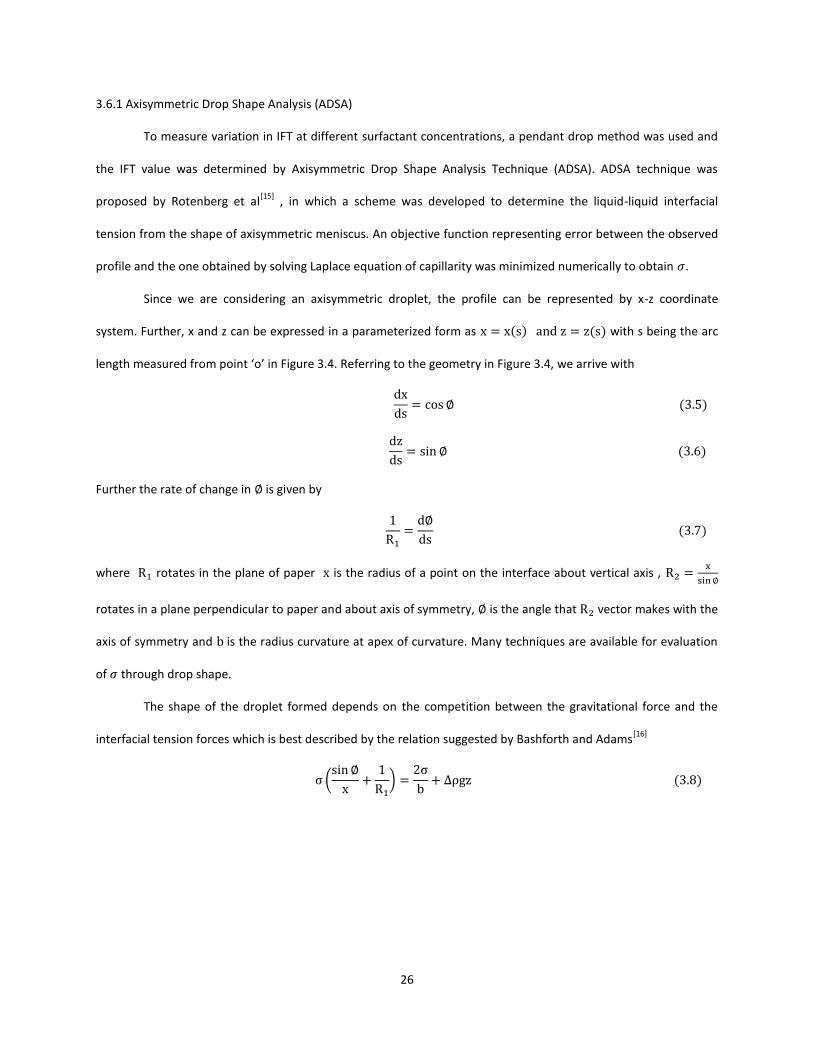
3.6.1 Axisymmetric Drop Shape Analysis (ADSA)

To measure variation in IFT at different surfactant concentrations, a pendant drop method was used and

the IFT value was determined by Axisymmetric Drop Shape Analysis Technique (ADSA). ADSA technique was

proposed by Rotenberg et al[15]

, in which a scheme was developed to determine the liquid-liquid interfacial

tension from the shape of axisymmetric meniscus. An objective function representing error between the observed

profile and the one obtained by solving Laplace equation of capillarity was minimized numerically to obtain .

Since we are considering an axisymmetric droplet, the profile can be represented by x-z coordinate

system. Further, x and z can be expressed in a parameterized form as ( ) ( ) with s being the arc

length measured from point ‘o’ in Figure 3.4. Referring to the geometry in Figure 3.4, we arrive with

( )

( )

Further the rate of change in is given by

( )

where rotates in the plane of paper is the radius of a point on the interface about vertical axis ,

rotates in a plane perpendicular to paper and about axis of symmetry, is the angle that vector makes with the

axis of symmetry and is the radius curvature at apex of curvature. Many techniques are available for evaluation

of through drop shape.

The shape of the droplet formed depends on the competition between the gravitational force and the

interfacial tension forces which is best described by the relation suggested by Bashforth and Adams[16]

(

)

( )

27

Figure 3.4 IFT measurement using ADSA technique from Profile of a pendant drop (Rotenberg et al

[15])

Combining equations 3.7 and 3.8 we get

( )

The profile of the droplet can be obtained by integrating the above differential equations with boundary

conditions ( ) ( ) ( ) .The experimental measured curve and the profile obtained by solving

equations are utilized to define an objective function which describes the error between the two profiles. If profile

form experiment is defined by , which represents points on interface and if ( ) is the profile from

calculated Laplacian solution then objective function can be expressed as [15]

⁄ ∑ [ ( )]

(3.10)

where ( ) is the normal distance between the curves and . The error E is minimized through appropriate

optimization procedure and correct value of is obtained.

3.6.2 Dynamic and Equilibrium IFT

In a system containing a surfactant either in continuous or dispersed phases, transport of surfactant from

bulk portion of phase containing it to the interface occurs entirely by the process of diffusion. During the formation

of pendant droplet the dispersed phase is injected into quiescent medium at a very slow rate and hence the

convective currents are fairly weak. Once a droplet is formed at tip of the capillary nozzle, IFT measurements are

made. When the interface is free from the surfactant the interfacial tension has value corresponding that of pure

system often represented by . However, with transportation of surfactant molecules to the interface, the

properties of interface changes and the interfacial tension drops. The lowering of interfacial tension depends on

the surface concentration of the surfactant and is given by Szyszkowski equation described earlier in the chapter.

Thus, as more and more surfactant molecules get adsorbed on to the interface, a further fall in values of interfacial

28

tension is observed. This time dependent variation in values of IFT is termed as ‘dynamic IFT’. After long time of

exposure of droplet to surfactant environment, equilibrium is attained and IFT approaches a steady value which is

termed at Equilibrium IFT. As equilibrium IFT can be attained only after a long time, a method proposed by Hunsel

et al. [17]

is normally used to estimate the equilibrium IFT value from the dynamic IFT data. The method is based on

the fact that the main mechanism guiding the transport of surfactant is diffusion. The suggested method involves

plotting dynamic IFT against

⁄ and extrapolating the curve to .

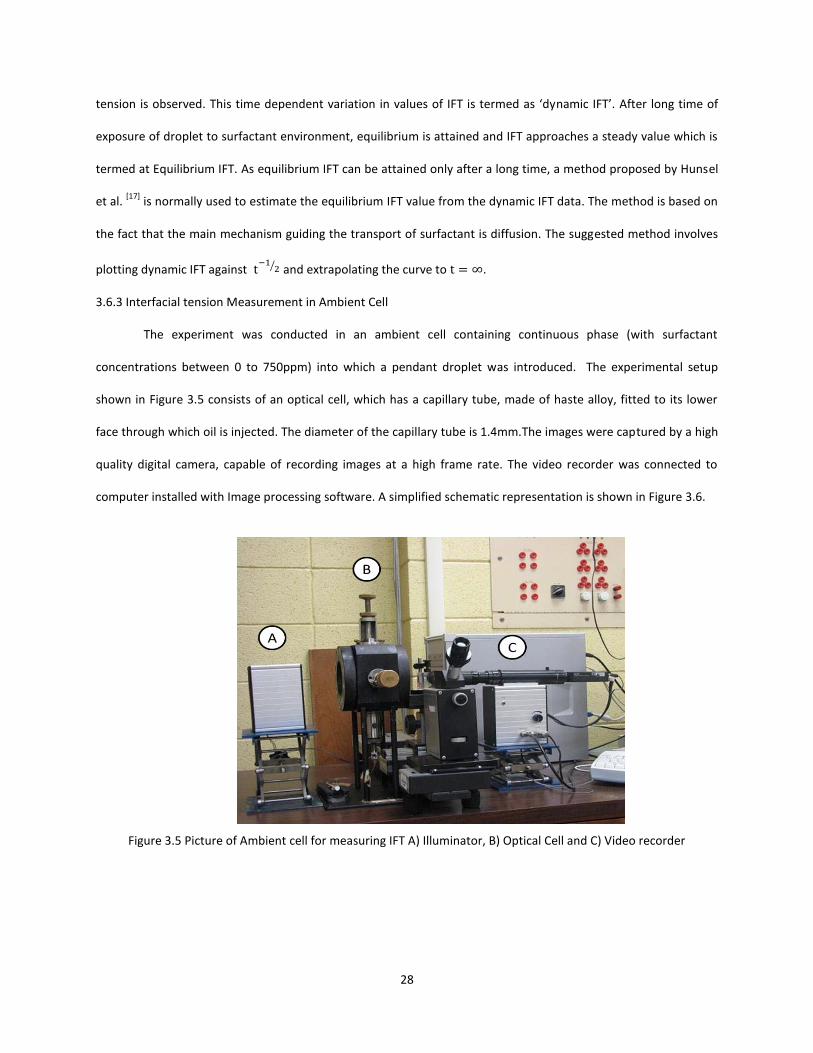
3.6.3 Interfacial tension Measurement in Ambient Cell

The experiment was conducted in an ambient cell containing continuous phase (with surfactant

concentrations between 0 to 750ppm) into which a pendant droplet was introduced. The experimental setup

shown in Figure 3.5 consists of an optical cell, which has a capillary tube, made of haste alloy, fitted to its lower

face through which oil is injected. The diameter of the capillary tube is 1.4mm.The images were captured by a high

quality digital camera, capable of recording images at a high frame rate. The video recorder was connected to

computer installed with Image processing software. A simplified schematic representation is shown in Figure 3.6.

Figure 3.5 Picture of Ambient cell for measuring IFT A) Illuminator, B) Optical Cell and C) Video recorder

29

Figure 3.6 Schematic diagram of experimental setup for IFT measurement

The continuous phase (water) containing surfactant is drawn into the optical cell through gravity. Once

the cell is filled, oil is injected slowly by a syringe, to form an axisymmetric pendant drop at the tip of the capillary

tube. The images of the pendant droplet are used to obtain the interface profiles. The interfacial tension is

computed by fitting a curve respecting Laplace equation of capillarity, to the shape and profile of the pendant

drop. The curve fitting exercise was done by the image analysis software. More details can be found in Rio et al

[18]. To obtain high quality results, the pendant drop technique requires extreme cleanliness. Hence, before each

experiment, entire system is thoroughly cleaned with toluene, acetone and distilled water and dried with a stream

of dry air, to ensure a contaminant free system. All IFT measurements in the present study are done at 298K. The

plot for dynamic IFT for oil-water interface at 100 ppm concentration SDS in continuous phase is shown in Figure

3.7. Figure 3.8 shows the static pendant drops formed at the tip of capillary nozzle at different surfactant

concentrations. If the IFT values are measured for a long time, steady equilibrium value is reached.

Figure 3.7 Dynamic IFT for SDS concentration of 100ppm

30

Figure 3.8 Static axisymmetric pendant droplets at various surfactant concentrations

Equilibrium values of IFT were extracted from dynamic IFT data by plotting dynamic IFT against

⁄ and

extrapolating the curve to . Figure 3.9 demonstrates the procedure followed in obtaining equilibrium IFT

values.

Figure 3.9 Extraction of Equilibrium IFT from dynamic IFT data as suggested in Hunsel et al[17]

Figure 3.10 shows a plot of Equilibrium IFT v/s the surfactant concentration in continuous phase. Clearly,

the IFT reduces with increase in concentration of surfactant SDS. However, there exists a value, beyond which a

further increase in concentration does not change the IFT. Such a concentration is called critical micelle

concentration (CMC, not shown in Figure 3.10). In present study, the concentrations of surfactant in the

continuous phase were much lesser than the CMC limit. Curve fitting of the above obtained experimental data

(i) (ii) (iii)

(a)

(b)

σ = 20.38 mN/m σ = 9.42 mN/m σ = 5.70 mN/m σ = 2.29 mN/mσ = 7.74 mN/m

0 ppm 100 ppm 250 ppm 500 ppm 750 ppm

31

with Szyszkowski equation given by Eq. 3.1 yields m ,maximum surface concentration and K , Langmuir adsorption

constant; the values were found to be .45 10-7 mol/m2 and 78.8 m

3/mol respectively.

Figure 3.10 Equilibrium IFT as function of SDS concentration

3.6.4 Diffusion controlled adsorption model

The transport of surfactant from the bulk phase, in the case of a static droplet, is purely by diffusion which

is followed by its adsorption. The molecules experience two resistances – one due to diffusion (transfer from bulk

phase to subsurface) and another due to adsorption-desorption process (when molecules are transported from

sub-surface to interface). Since diffusion is a slow process (for a stagnant system diffusion length is infinite[19]

), the

time taken for attaining equilibrium surface concentration is fairly long. However, when the droplets are in motion,

the convective flux is more dominant than the diffusive flux at the surface of droplet. This helps in a quick and an

efficient delivery of surfactant molecules to the sub-surface (region near the interface with few molecular

thickness) from the bulk fluid and hence the time taken to reach an equilibrium adsorption state should be much

lesser. At this point, it would be pertinent to estimate the time required to attain the saturation concentration at

the interface through adsorption when the droplet is moving. To address this we have used the dynamic

adsorption controlled model suggested in Chang et al.[19]

In this model it is assumed that the diffusion is the only

mechanism required for establishing adsorption equilibrium. Unlike in case of a stagnant droplet, for a moving

droplet, existing convection reduces the diffusion length ‘l’ to a finite value. Thus, the time taken to reach

0

5

10

15

20

25

0.000001 0.00001 0.0001 0.001 0.01

IFT

(mN

/m)

SDS concentration (mM)

32

equilibrium state depends on the adsorption timescale(described in Chang et al.[20]

) and is very less than that for a

stagnant system. The diffusion length has been approximated to adsorption depletion length given by

l m

C0⁄ (3.11)

where is the concentration in the continuous phase. The adsorption timescale depends on the dimensionless

length l mK ⁄ .The time required for the surface concentration to attain 95% of equilibrium concentration (has

been discussed in Chang et al.[20]

)is given by,

t95 C95 [l( mK )

D⁄ ] for l mK ⁄ 1 (3.12)

t95 [( mK )

2

D⁄ ] for l mK

⁄ 1 (3.13)

where C95 and are function of dimensionless concentration C0K . In Eq. 3.12, C95 can be evaluated by

C95 1 C0K ⁄ , as suggested in Chang et al

[20]. D is the diffusivity of the surfactant in bulk phase. Table 3.3 shows the

details pertaining to the adsorption length and time required to reach an equilibrium state. It can be seen that the

time taken to reach the 95% of saturation surface concentration is far less than the time spent by droplet in the

column (which was around 10-15s). Hence, during the development of the numerical model we have assumed that

the interfacial tension at oil/water interface was constant at its equilibrium IFT value. Further, because of this fairly

fast kinetics of the surfactant, it can be safe to ignore Marangoni stresses along the surface of the droplet.

Table 3.3 Time required for surface concentration to reach 95% of equilibrium surface concentration

(ppm) (mol/m3) (m) (s)

3.7 Mathematical Model

In this section, the capabilities of Computational Fluid Dynamics in simulating experimental observations

are explored. A numerical model based on finite volume method was developed using a commercially available

code, ANSYS Fluent®. It was observed in the experiment that the smaller droplets exhibited axisymmetric behavior

33

and traced a rectilinear path. To save on computational effort in such cases two-dimensional axisymmetric

simulations were performed on these droplets. The larger droplets travelled in a zigzag path and were simulated

using complete 3D simulations.

The numerical model was formulated with following assumptions;

1) The fluids involved are immiscible, viscous, incompressible and Newtonian.

2) The flow is isothermal.

3) The interfacial tension across the interface was assumed to bear a constant value (equilibrium IFT).

4) The oil/water interface is assumed to be mobile.

The process of droplet formation was not considered for numerical investigation. In these simulations,

droplets were released from rest and allowed to rise in the domain. The size of the computational domain was

large enough to ensure that wall had no influence on the rising droplet.

3.7.1 Governing Equations

Many methods have been suggested in literature for simulating multiphase flow and subsequent tracking

interfaces. Few examples are, VOF method ,[21]

Marker and cell method, [22]

Front Tracking Method,[23]

Level Set

Method[24]

etc. In this study, Volume of fluid (VOF) method proposed by Hirt et al.[21]

has been used to simulate

the hydrodynamics of the droplets rising in the column. In this study, we have used VOF method conjugated with

an interface reconstruction technique based on piecewise linear interface (PLIC)representation[25]

for simulating

the motion of the droplet in the water column. VOF is advantageous over other methods for they are relatively

simple, robust, accurate and account for substantial topological changes in the interface. [26]

A single momentum

equation along with the continuity equation is solved in the entire domain and the calculated velocity field is

shared between the phases.

( )

(3.14)

( ) ( ) [ ( ]

(3.15)

where and are the volume fraction averaged properties given by ∑ ∑ where is the

volume fraction of phase ‘q’. accounts for the body forces; in current case it refers to force due to interfacial

tension, which is calculated according continuum surface force (CSF) model[10]

given by

34

⟨ ⟩⁄ (3.16)

where is surface tension coefficient, is local surface curvature given by

(3.17)

with being unit surface normal vector given by | |⁄ . The CSF is included in the momentum equation,

so that the momentum equation satisfies the stress balance boundary condition on the interface.

3.7.2 Interface tracking in VOF method

The above formulation has been developed for two or more fluids which are immiscible. A phase is

represented by volume of fraction . A value of =1 represents a dispersed phase whereas represents a

continuous phase. Interface is a represented by a diffused region where takes values between 0 and 1. The

method is naturally conservative, has a fast convergence and a reasonable accuracy [27]

. The VOF method works on

a fixed grid and the position of interface is determined by the solution of a scalar balance equation for the volume

fraction of dispersed phase

( )

(3.18)

The accuracy of the volumetric interfacial tension force appearing as source term in the momentum

equation (Eq. 3.17) depends on the proper evaluation of the curvature. In this study, we have used the VOF

gradients directly from the nodes which is conjugated with node based smoothing of VOF field for accurate

evaluation of the curvature. This results in a better estimation of surface tension force than that calculated using

the VOF gradients at the cell centers.

3.7.3 Geometric reconstruction scheme

Geometric reconstruction scheme represents the interface in a piecewise linear manner which is shown in

Figure 3.11. This method known as PLIC ( Piecewise linear interface calculation) was developed by Young et al. [28]

.

It is based on the assumption that the interface in each cell has a linear slope and this shape of the interface is

used for calculation of advection of fluid through the cells in the computational domain (Figure 3.11). The first step

in this scheme involves calculating the position of the linear interface relative to the center of each partially- filled

cell (cell containing both dispersed as well as continuous phases), based on the information about the volume

fraction and its derivatives in the cell. In the second step is the amount of fluid advecting through each face is

35

evaluated using the computed linear interface representation and information about the normal and tangential

velocity distribution on the face. The last step involves calculation of volume fraction in each cell by utilizing

balance of fluxes evaluated in the earlier step.

Figure 3.11 (a) Actual Interface, (b) Interface represented by geometric reconstruction (piecewise linear) scheme

3.7.4 Numerical methods and simulation setup

The transient simulation was carried out using explicit scheme. Geometric Reconstruction scheme was

used for constructing interfaces in the cells where varied between 0 and 1 (representing interface). The explicit

scheme is advantageous as it renders a clear, crisp interface without numerical diffusion. It is preferred in

simulation of flows where surface tension is important because of highly accurate curvature calculation. The

pressure velocity coupling was established using PISO (Pressure –implicit with splitting of operators) scheme. The

spatial discretization used in momentum equation was second order upwind differencing scheme. The calculation

of gradients was based on the Green-Gauss Cell Based method. PRESTO (Pressure Staggering Option) scheme was

employed for pressure interpolation.

The computational domain consists of a small section [( )

] for 3D case and [( ) ] for 2D axisymmetric case, where R refers to the

radius of the droplet. The computational domain for simulation alongwith the boundary conditions have been

shown in Figure 3.12. For 2D axisymmetric case, triangular meshing was done over the domain using ANSYS ICEM.

More details on the simulation have been summarized in Table 3.4. For 3D simulations a domain containing

tetrahedral elements was constructed. The wall boundary condition imposes no slip (all components of velocities

are zero) at the lower face of the computational domain.

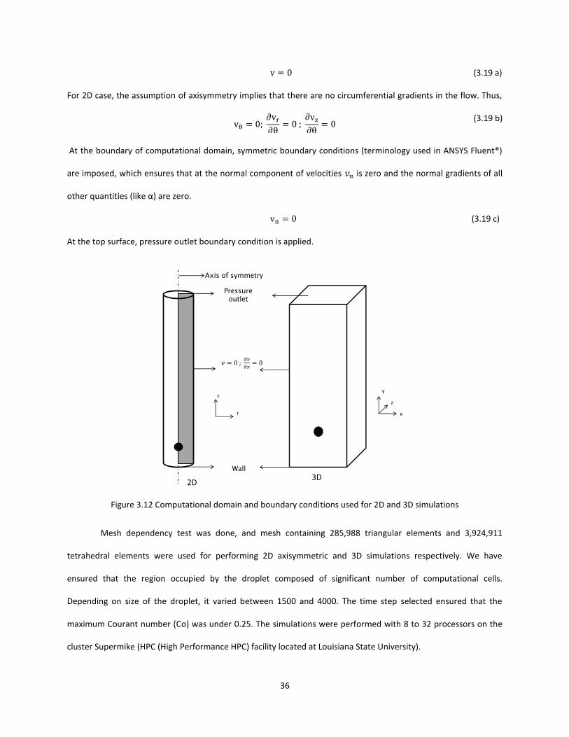
36

(3.19 a)

For 2D case, the assumption of axisymmetry implies that there are no circumferential gradients in the flow. Thus,

(3.19 b)

At the boundary of computational domain, symmetric boundary conditions (terminology used in ANSYS Fluent®)

are imposed, which ensures that at the normal component of velocities is zero and the normal gradients of all

other quantities (like α) are zero.

(3.19 c)

At the top surface, pressure outlet boundary condition is applied.

Figure 3.12 Computational domain and boundary conditions used for 2D and 3D simulations

Mesh dependency test was done, and mesh containing 285,988 triangular elements and 3,924,911

tetrahedral elements were used for performing 2D axisymmetric and 3D simulations respectively. We have

ensured that the region occupied by the droplet composed of significant number of computational cells.

Depending on size of the droplet, it varied between 1500 and 4000. The time step selected ensured that the

maximum Courant number (Co) was under 0.25. The simulations were performed with 8 to 32 processors on the

cluster Supermike (HPC (High Performance HPC) facility located at Louisiana State University).

Pressure outlet

Wall

Axis of symmetry

z

r

2D

z

x

y

3D

37

Table 3.4 Numerical simulation specifications

Dispersed Phase Continuous Phase

Crude Oil Water

Density 888.84 kg/m

3

999.5 kg/m3

Viscosity 25.25 cP 1 cP

Simulation Parameters

Domain Size 0.08 m X 0.25 m

Number of cells 285,988 (2D axisymmetric) 3,924,911 (3D)

Model Volume of Fluid

3.8 Observations and Discussion

3.8.1 Experiment

3.8.1.1 Effect of surfactant on the size of droplet formed at the nozzle

During each of the runs, the droplets were injected at a low flow rate, to suppress the contribution of

inertial force. When the crude oil is injected in the tank, the droplet initially grows at the tip of nozzle. Under static

conditions, the pinch off mechanism of the droplet is governed by balance between buoyancy force, gravitational

force and interfacial tension force at the nozzle tip. The droplet grows until it acquires enough buoyancy to

overcome the interfacial tension and ultimately pinches off.[29]

It can be seen in Figure 3.13 that as the surfactant concentration is increased, the size of the droplet

produced at the nozzle decreases. The actual images just before pinch off for different surfactant concentrations

can be found in Figure 3.8. One possible explanation is that, with lowering interfacial tension the interfacial tension

force on the droplet at nozzle decreases. So, the net buoyancy required for the droplet to pinch off falls and this

results in formation of a smaller sized droplet. Figure 3.13 also depicts a good agreement between the size of

droplet observed in the experiment with that predicted by Eq. 12 and deviation is under 12%.

38

Figure 3.13 Dependence of droplet size on the surfactant concentration and its comparison with Eq. 3.3

3.8.1.2 Effect of surfactant on the trajectory and shape of the droplet

The trajectory adopted by the droplets, during their rise, is primarily dependent on their shape, which in

turn is function of the Re, Eo and M.[5]

The interfacial tension force acts as a restoring force whereas as inertial and

shear forces have a tendency to distort the droplet. The wake structure also influences the droplet’s path. It was

observed that the smaller droplets (< 5mm) assumed ellipsoidal shape and moved in rectilinear paths. These

droplets were seen to exhibit axisymmetry even at higher concentrations of the surfactant. However, the larger

droplets (> 6mm) were initially found to assume ellipsoidal shape at the point of release but became more

distorted as they rose in the water column, when surfactant was adsorbed on to its surface. These droplets

exhibited oscillations about the horizontal plane and were found to travel in zigzag path.

Figure 3.14 shows the trajectories taken by the droplets emerging from nozzle A1, A2 and A3

respectively, in a medium without surfactant and the one having 750 ppm concentration. The snapshot reveals

the position of droplet after every 0.03s. As evident from the figure, in absence of a surfactant, most of the

droplets rise in a rectilinear path; even the larger droplets (corresponding to Re ≈ 900) adopt a slightly zigzag

path. However, at high surfactant concentration, even the smaller droplets adopt a zigzag trajectory and droplets

with higher Reynolds number (> 300) begin to oscillate about their axes of motion moving in a zigzag path. Table

3.5 summarizes the observed trajectories of droplets at different surfactant concentrations.

0

0.1

0.2

0.3

0.4

0.5

0.6

0.7

0.8

0.9

0 200 400 600 800

Dia

me

ter

(cm

)

SDS concentration (ppm)

A3(experimental)

A3(correlation)

A2(experimental)

A2(correlation)

A1(experimental)

A1(correlation)

39

Figure 3.14 Trajectory of droplets in (a) absence of surfactant and (b) surfactant concentration 750 ppm

The path taken by the droplets depends on the structure of wake at its trailing end. Various categories of

wakes that have been reported in literature[4, 30]

are steady wake without circulation, steady wake with circulation

and unsteady wake with vortex shedding[5, 31]

. The non-oscillating droplets which travel in straight path are

associated with wakes bearing axisymmetric structure. However, at higher concentrations the droplets undergo

significant deformation which results in formation of asymmetric wakes. These wakes are responsible for the

wobbling motion exhibited by the droplets in this regime which makes them travel in a zigzag path.

The flow around a droplet differs from that of rigid sphere, as the internal circulations inside the droplet

delays the flow separation and the subsequent wake formation in the surrounding fluid.[4]

This is true for fluid with

low and when system is relatively clean. In present case, is pretty high and for system with high surfactant

concentration one can expect that the onset of wake and the oscillations to happen at a much lesser Re.[32]

This

can be noticed in the Table 3.5; with increase in surfactant concentration, the droplet departs from rectilinear path

at Re as low as 200. More details on this will be given in the section describing the results from the simulation.

Table 3.5 Trajectories of droplets depending on M and Re (Values in bracket indicate corresponding Re)

(a) (b)

Nozzle/Surfactant concentration(ppm)

Morton Number(M)

A1 A2 A3

Rectilinear(469) Rectilinear(661) Slightly zigzag(897)

100 Rectilinear(416) Rectilinear(610) Oscillating-Zigzag(786)

250 Rectilinear(363) Rectilinear(538) Oscillating-Zigzag(679)

500 Rectilinear(264) Oscillating-Zigzag(367) Oscillating-Zigzag(458)

750 Slightly zigzag(202) Oscillating-Zigzag(296) Oscillating-Zigzag(370)

40

3.8.1.3 Aspect Ratio

The shape assumed by the droplet rising in the water column is governed by the competition between

interfacial tension and shear due to flow around droplet. The images in Figure 3.15 are actual snapshots from the

experiment, which illustrate the impact of surfactant on the shape of droplet, produced from nozzle A3.

Figure 3.15 Effect of surfactant on the aspect ratio of droplets from nozzle A3

In absence of a surfactant, the flattening of oil drops at the front end can be attributed to the increased

hydrodynamic pressure, which can be associated to the stagnation point at the upper surface of the droplet. The

lower surface of the oil droplet appears more spherical because of the more uniform distribution of the pressure.

When a droplet rises in the medium with surfactant, surfactants are adsorbed on to the surface gradually. Due to

this build up in surfactant concentration, the interfacial tension is lowered and the shear stresses imposed by the

surrounding fluid causes the droplet to stretch by a greater extent, and the droplet elongates in transverse

direction to acquire a flatter shape. Thus, a reduction in the value of aspect ratio is observed. For the range of

concentration of surfactant used in experiment, it was observed that the aspect ratio of the droplets gradually

decreased with increase in surfactant concentration in the continuous phase. The actual snapshots of the droplets,

at various concentrations of surfactant are shown in Figure 3.16. A scan from bottom to top in each of the column

indicates the reduction in aspect ratio of the droplet (as stated earlier this occurs in conjugation with decrease in

droplet size) with the increase in surfactant concentration.

0 ppm 250 ppm 750 ppm

41

Figure 3.16 Effect of surfactant on the aspect ratio of droplets from nozzle A3

Many correlations have been developed to estimate the aspect ratio for ellipsoidal droplets. The aspect

ratio exhibited by the droplets in the experiment has been compared with that obtained from a correlation

developed by Vakrushev and Efremov[33]

, which estimates the degree of deformation of droplet on basis of its

Tadaka Number (Ta) which is given by

Ta Re (3.20)

In present study, Ta was in the range 2 Ta 9.

E [0. 1 0.20 tanh{2(0. - log10 Ta)}]3 (3.21)

This has been depicted in Figure 3.17 and it can be found that the shape acquired by the droplets in the

experiment is pretty close to the predicted values.

750 ppm

500 ppm

250 ppm

100 ppm

0 ppm

A1 A2 A3

42

Figure 3.17 Comparison of the droplet aspect ratio observed with that predicted from Eq. 3.21

3.8.1.4 Effect of surfactant on Rise Velocity of droplet

Whenever a droplet is released into stagnant medium, it initially accelerates. Eventually, a balance is

established between the drag, buoyancy and gravitational forces and the droplet attains terminal velocity. For a

droplet undergoing no mass loss, the volume can essentially be assumed to remain constant. Thus, the buoyancy

and gravitational forces remain constant and thus, under such circumstances the rise velocity of the droplet solely

depends on the magnitude of the drag force. The drag force is dictated by the shape of droplet and also on the

influence of the surfactant on the motion of fluid inside the droplet. The effect of surfactant addition on the

average rise velocity for droplets at different surfactant concentrations has been shown in Figure 3.18, a. It can be

noticed that the average rise velocity of a particular sized droplet decreases with increase in surfactant

concentration. This decrease in rise velocity can be attributed to the reduction in size of droplet as well as that in

aspect ratio due to the lowering of interfacial tension at the oil water interface. The flatter droplets witness an

increase in drag force which contribute to their lower rise velocity.[34]

The dynamic rise velocity of droplets from

A3 nozzle has been shown in Figure 3.18, b. It can be observed that the rise velocity settles to a steady value in for

droplet rising in medium containing no surfactant. On the other hand, the droplet moving in a high surfactant

concentration environment acquires an oscillatory behavior and exhibits fluctuations in rise velocity about a value.

0

0.1

0.2

0.3

0.4

0.5

0.6

0.7

0.8

0.9

0 0.2 0.4 0.6 0.8 1

Asp

ect

rat

io

Droplet diameter (cm)

0 ppm (experiment)

250ppm(experiment)

750ppm(experiment)

0ppm(theory)

250ppm(theory)

750ppm(theory)

43

In current study the viscosity ratio Ƙ is 25. Consequently, the internal circulations developed inside the droplet are

not very strong (ratio of maximum internal circulation to Droplet velocity is less than 15%). And hence one can

expect that the magnitude by which the drag force increases due to the weakening of internal circulations in

presence of surfactant will not be tremendous. Thus, in the present study, it would not be very incorrect to believe

that the major contributor towards drag enhancement is the distortion experienced by the droplet due to the

reduction in the interfacial tension.

Figure 3.18 Effect of surfactant on the rise velocity of droplet (a) Average rise velocities as a function of SDS concentration compared with Eq. 3.23. (b) Dynamic rise velocities of droplets from nozzle A3

The hydrodynamic drag force can be calculated by,

⁄

(3.22)

where refers to the projection area , the cross- sectional area of the droplet in the direction normal to the

motion of the droplet. can be evaluated from buoyancy and the gravitational force acting on the droplet.

The values of for droplets thus obtained have been plotted in Figure 3.19, a., at various M. It shows

that, for a particular sized droplet, the drag coefficient increases with the increase in M, which can be attributed to

increase in oblateness. The effect of surfactant on the drag coefficient is highest at the transition point, where

motion changes from rectilinear to oscillatory. [4, 5]

This can be seen in Figure 3.19, b., which shows that at

transition point, (which is demarcated by a solid curve passing through all curves), the value of increases. The

drag contribution in region where droplet remains ellipsoidal and rises in rectilinear trajectory is mainly due to

0

2

4

6

8

10

12

0 0.2 0.4 0.6 0.8 1

Ris

e v

elo

city

(cm

/s)

Droplet diameter (cm)

0ppm(exp)

250ppm(exp)

750ppm(exp)

0ppm(theory)

250ppm(theory)

750ppm(theory)

0

2

4

6

8

10

12

0 2 4 6 8 10

Ris

e v

elo

city

(cm

/s)

Time t (s)

No surfactant

750 ppm

(a)

(b)

0

2

4

6

8

10

12

0 0.2 0.4 0.6 0.8 1

Ris

e v

elo

city

(cm

/s)

Droplet diameter (cm)

0ppm(exp)

250ppm(exp)

750ppm(exp)

0ppm(theory)

250ppm(theory)

750ppm(theory)

0

2

4

6

8

10

12

0 2 4 6 8 10

Ris

e v

elo

city

(cm

/s)

Time t (s)

No surfactant

750 ppm

(a)

(b)

44

viscous drag. However, beyond transition point, where droplets exhibit oscillations contribution of pressure drag

and energy loss due to oscillations, contribute much more to the total drag and hence increases drastically.[4]

Figure 3.19 Effect of surfactant on drag coefficient (a) Cd as function of droplet diameters at various Morton

numbers (M) (b) Cd variation as a function of Re at various Morton Numbers(M)

The rise velocities observed in the experiment were compared with the expression suggested by Clift et al.[5]

,

c dp

0.149 ( 0. 57) (3.23)

where 0.94 H0.757 for (2 H 59.3)and 3.42H0.441 for (H 59.3) , with 4 3 ⁄ Eo -0.149 ( c

w⁄ )

-0.14

and

w 0.009Pa.s.

As can be seen in Figure 3.18, a., the observed velocities closely followed the velocities predicted from

the above correlation.

3.8.2 Numerical Results

One of the prime requirements of the numerical model developed is to simulate the deformations

observed in the experiment. In our numerical study, we have not considered the actual droplet formation process,

rather a region equivalent to the size of the droplet observed in the experiment was marked in the computational

domain and assigned a value of , to represent dispersed (oil) phase and the droplet was allowed to start

from the rest. The diffusion controlled adsorption model, presented in the earlier sections, suggested that the

time required for interface to attain saturation surfactant concentration was a small fraction of the total time

spent by the droplet in the column. In this study, we do not simulate the actual adsorption process of surfactant

rather we assume that the oil/water interface bears constant interfacial tension equal to its equilibrium value

0.5

0.55

0.6

0.65

0.7

0.75

0.8

0.85

0.9

0.95

1

0.2 0.3 0.4 0.5 0.6 0.7 0.8 0.9

Dra

g co

eff

icie

nt

Cd

Droplet diameter (cm)

A3

A2

A1

0

0.1

0.2

0.3

0.4

0.5

0.6

0.7

0.8

0.9

1

0 200 400 600 800 1000

Dra

g C

oe

ffic

ien

t C

d

Re

M=1.28E-10

M=1.30E-09

M=2.34E-09

M=5.87E-09

M=9.05E-08

Wobbling regime

Ellipsoidal regime

(a)

(b)

0.5

0.55

0.6

0.65

0.7

0.75

0.8

0.85

0.9

0.95

1

0.2 0.3 0.4 0.5 0.6 0.7 0.8 0.9

Dra

g co

eff

icie

nt

Cd

Droplet diameter (cm)

A3

A2

A1

0

0.1

0.2

0.3

0.4

0.5

0.6

0.7

0.8

0.9

1

0 200 400 600 800 1000

Dra

g C

oe

ffic

ien

t C

d

Re

M=1.28E-10

M=1.30E-09

M=2.34E-09

M=5.87E-09

M=9.05E-08

Wobbling regime

Ellipsoidal regime

(a)

(b)

45

corresponding to the bulk surfactant concentration. Since the system under consideration has a high concentration

of surfactant, and because of fairly fast kinetics of the surfactant, the role of Marangoni convection has been

ignored.

3.8.2.1 Comparison of Simulation results with Experimental Observations

The simulations were carried out by using commercial CFD code ANSYS® Fluent. The shapes of the

droplet predicted from 2D and 3D model described in the section 3.7.1, were in good agreement with that

observed in the experiment. This has been depicted in the Figure 3.19, a. and 3.19, b.

Figure 3.19 Comparison of droplet shape predicted from numerical simulation with images from experiment (a) 2D

axisymmetric case (b) 3 D simulation, the centre row represents the mid-section view of 3D droplet

Figure 3.20 show the results from 2D and 3D simulations which depict the decrease of aspect ratio and

rise velocity of droplet with increase in surfactant concentration in the continuous phase. It can be seen that the

model does a good job in predicting the trend similar to that observed during experiment. The match between the

rise velocities and aspect ratio for 2D and 3D simulation; with that exhibited by droplets during the experiment is

pretty satisfactory with error of less than 10%.

750 ppm250 ppm0 ppm

(a)

(b)0 ppm

500 ppm

250 ppm

100 ppm

750 ppm

Experiment 2D simulation

46

Figure 3.20 Comparison of (i) Average rise velocity v/s SDS concentration for 2D axisymmetric simulation (ii) Aspect ratio velocity v/s SDS concentration for 2D axisymmetric simulation (iii) Average rise velocity v/s SDS concentration

for 3D simulation (iv)Aspect ratio velocity v/s SDS concentration for 3D simulation with experimental data.

3.8.2.2 Pressure distribution and stagnation point

Figure 3.21, a., from 3D simulations, shows the distribution of the pressure coefficient around the droplet.

It can be seen from the contour plot that the stagnation point is at the upper pole of the moving droplet; thus

pressure coefficients bear a higher value at the upper surface than on the lower part of the droplet. Figure 3.21, b.

depicts the variation of total pressure along the surface of the 2D axisymmetric droplet rising in the environment

with different surfactant concentrations. The angle θ is measured from the front stagnation point. It can be seen

that as the droplet becomes flatter with increase in surfactant concentration, the pressure recovery along the

surface reduces.

0

2

4

6

8

10

12

0 200 400 600 800

Ave

rage

ris

e v

elo

city

(cm

/s)

SDS concentration (ppm)

Experiment

CFD

0

0.1

0.2

0.3

0.4

0.5

0.6

0.7

0.8

0.9

1

0 200 400 600 800

Asp

ect

Rat

io

SDS concentration (ppm)

Experiment

CFD

0

0.1

0.2

0.3

0.4

0.5

0.6

0.7

0.8

0.9

1

0 100 200 300 400 500 600 700 800

Asp

ect

rat

io

SDS concentration (ppm)

Experiment

CFD

0

2

4

6

8

10

12

0 100 200 300 400 500 600 700 800

Ave

rage

ris

e v

elo

city

(cm

/s)

SDS concentration (ppm)

Experiment

CFD

2D simulation

3D simulation

(i)

(iii) (iv)

(ii)

47

Figure 3.21 (a) Pressure coefficients around droplet at various surfactant concentrations. (b) Variation of total

pressure across the surface of an axisymmetric droplet at different surfactant concentrations 0 ppm , 250 ppm and 750 ppm ; Corresponding Re are 469

Figure 3.22 shows the axial velocity vectors from 2D simulations. The right portion of each image shows

the associated vorticity contours. It can be seen that with increase in surfactant concentration the droplet

becomes flatter. The oblateness imparted due to the presence of the surfactant reduces the angle of flow

separation (measured from the front stagnation point) and the separation ring shifts towards upper pole.

Consequently, the recirculating wake formed at the rear end of the droplet due to vorticity accumulation widens

and reduces in length (wake length is measured from rear of the droplet to the point where the recirculation

ends). For the simulated droplets, wake length for a droplet with no surfactant (Re= 470) was 0.011m whereas for

750 ppm case (Re= 200), it was about 0.008m. It was observed that the ratio of maximum circulation velocities to

the droplet rise velocity decreased by nearly two folds as the surfactant concentration was increased from 0ppm

to 750ppm.

0 ppm 250 ppm 750 ppm

0

2

4

6

8

10

12

0 50 100 150 200

Tota

l Pre

ssu

re (

N/m

2 )

θ(Degrees)

0 ppm

250 ppm

750 ppmStagnation point

(a)

(b)

θ

Stagnation point

48

Figure 3.22 Velocity vectors and vorticity contours in simulated droplets at various surfactant concentrations for

2D axisymmetric case

3.8.2.3 Droplet Trajectory and Wake structure

We have seen in previous sections that the larger droplets from nozzle A3 and relatively smaller droplets

in higher surfactant concentration environment exhibit zig-zag trajectory. The change in the trajectory of droplet

,i.e. from rectilinear to zigzag, at higher surfactant concentrations can be attributed to the oblateness imparted to

the droplet which changes the characteristics of wake, formed behind the droplet.[35]

Figure 3.23, a. shows the

evolution of wake structure as the droplet (from nozzle A3) travels in a medium with 750 ppm SDS concentration.

It has been stated that unlike in case of a rigid sphere boundary layer separation is delayed in fluid sphere , and

this is evident from the flow structure around the spherical droplet at t=0.02s. It can be seen that even at Re=64 ,

flow separation fails to occur ( For rigid , flow separation is observed at a Re ≈20[5]

). However, at a higher Re=335,

the droplet deforms and one can observe flow separation and two vortices are formed at the rear end of the

droplet which are symmetrical nature. At this instant the droplet rises in a straight path. The axisymmetric

behavior of wake begins to break when the detachment of right vortex commences (Re=348). At Re=372, the right

vortex completely detaches, and the pressure differences, at the rear of droplet, with larger area of lower pressure

at the left portion of droplet, forces it to move left. When Re =384 at end of t=1.2s, the vortex at left detaches and

the pressure gradient reverses and this pushes the droplet to move right. Thus, droplet exhibits a zig-zag motion.

Thus, the lateral movement of the droplet from the straight path can be attributed to the asymmetric nature of

wakes at rear of droplet which lead to pressure differences. It was observed that at higher surfactant

concentration, breaking of axisymmetric nature of the wake occurred at lower Re. This has been shown in Figure

0 ppm 250 ppm 750 ppm

49

3.24. Further, it can be noticed from the contour plot of pressure in Figure 3.23, a. that the stagnation point(

region of higher pressure) at upper face moves from centre to right as the droplet is forced to move left due to

asymmetric wakes. Figure 3.23, b. depicts the wake structure and contour of total pressure for a droplet exhibiting

axisymmetric behavior.

Figure 3.23 (a) Wake structure and total pressure distribution at various times for droplet moving in column with

750 ppm SDS (b) Wake structure for an axisymmetric droplet in 750 ppm surfactant concentration

(b)

(a)

0.02sRe=64

0.2sRe=335

0.3sRe=348

0.4sRe=361

0.5sRe=372

0.8sRe=385

1.0sRe=388

1.2sRe=384

1.6sRe=392

50

Figure 3.24 Loss of axisymmetric nature of wakes at different Re depending on the surfactant concentration

Figure 3.25 depicts the wake structure and associated vorticity magnitude for droplet travelling in the

medium with 250ppm SDS concentration. It was described earlier that the intermediate sized droplets exhibited

oscillations. The onset of oscillations occurs at a point when vortex shedding from the wake commences. It can be

seen that with increase in Re of the flattened droplet, the vorticity contours acquire more asymmetrical structure

and discrete parcels of vortices begin to shed from the wake and this sets in oscillations.

Figure 3.25 Vorticity magnitude contour plot at different Re for system with 250ppm SDS concentration

0 ppmRe=856

250 ppmRe=645

750 ppmRe=372

0.1sRe=317

0.2sRe=506

0.6sRe=644

1.0sRe=662

51

3.9 Conclusions

An experimental and numerical investigation was carried out to analyze the effect of surfactant on the

dynamics of crude oil droplet. Droplets ranging between 3 to 8 mm were produced from three different nozzles

and released into the quiescent water column, containing SDS surfactant. Smaller droplets at low surfactant

concentrations ascended in a rectilinear path whereas larger droplets and droplets in medium with high surfactant

concentration acquired a zig-zag path.

Pendant drop experiments were conducted in ambient cell for evaluating IFT at oil-water interface at

different surfactant concentrations employing ‘Axisymmetric drop shape analysis’ (ADSA) method. A diffusion

controlled model as described by Chang et al. [20]

was used to estimate the adsorption time for a moving droplet

and it was found that time required to saturate the interface was very small compared to the time spent by

droplet in the column. It was observed that the increase in bulk surfactant concentration lowered the interfacial

tension and this resulted in,

decrease in the size of droplet being generated at the tip of a particular nozzle;

decrease in aspect ratio of the droplet, i.e. droplets assumed a more flatter shape and

as a consequence, decrease in the rise velocities of the droplet was observed. The rise velocities and aspect ratio

observed in the experiment were found to agree well with relevant correlations listed out in Clift et al. [5]

Drag

coefficients were evaluated using simple force balance around the droplet and an increase in their value was

observed at higher surfactant concentrations. The rise was more pronounced droplets entered an oscillatory

regime.

In addition to the experiments, a numerical model was developed to simulate the behavior of droplets

observed in the experiment and the simulations were carried out in ANSYS Fluent® using VOF scheme. To reduce

the computational time, the droplets which were found to follow a rectilinear path were simulated using 2D

axisymmetric assumption. Larger droplets which deviated significantly from the axis and underwent oscillations

were simulated by a 3D model. The agreement between the rise velocities and shape predicted from the model

and those observed in the experiment was found to be satisfactory.

52

The evolution of wake structures at the rear of the droplet was studied and it was concluded that the

asymmetric wake pattern caused the droplets to travel in zigzag path. It was observed that with the increase in

bulk surfactant concentration, the onset of asymmetry in wake occurred at a lower Re and this corroborated with

the experimental observations. The flattening of droplet at higher surfactant concentrations also resulted in

shifting of point flow separation towards the upper pole of the droplet and as a result the angle of separation

(measured form the stagnation point on the upper face) increased.

3.10 Nomenclature

: Projected area of droplet in direction normal to its motion [m2].

: Drag coefficient

: Pressure coefficient

: Droplet diameter, [m].

: Diameter of nozzle, [m].

E : Aspect ratio

: Drag force, [N].

: Interfacial Tension force, [N].

: Total pressure, [N/m2].

: Average rise velocity of the droplet, [m/s].

: Volume of droplet at the time of formation [m3].

: Corrected volume of droplet after pinch off [m3].

Greek alphabets

: Volume of fraction of dispersed phase

: Surface curvature

: Viscosity ratio of dispersed phase to that of continuous phase

: Density of continuous phase [kg/m3].

: Density of dispersed phase [kg/m3].

: Viscosity of continuous phase [kg/m.s].

53

: Viscosity of dispersed phase [kg/m.s].

: Harkins Brown Factor

Non dimensional Number

: Reynolds Number

: Eötvos Number

: Morton Number

: Tadaka Number

3.11 References

[1] E.B. Kujawinski, M.C. Kido Soule, D.L. Valentine, A.K. Boysen, K. Longnecker, M.C. Redmond, Fate of Dispersants Associated with the Deepwater Horizon Oil Spill, Environmental Science & Technology, 45 (2011) 1298-1306.

[2] F.H. Garner, A.H.P. Skelland, Some factors affecting droplet behaviour in liquid-liquid systems, Chemical Engineering Science, 4 (1955) 149-158.

[3] F.H. Garner, A.R. Hale, The effect of surface active agents in liquid extraction processes, Chemical Engineering Science, 2 (1953) 157-163.

[4] S. Winnikow, B.T. Chao, Droplet Motion in Purified Systems, Physics of Fluids, 9 (1966) 50-61.

[5] R. Clift, J.R. Grace, M.E. Weber, Bubbles, Drops, and Particles, Dover Publications, Mineola,NY, 2005.

[6] Y. Wang, D.T. Papageorgiou, C. Maldarelli, Increased mobility of a surfactant-retarded bubble at high bulk concentrations, Journal of Fluid Mechanics, 390 (1999) 251-270.

[7] L.-H. Chen, Y.-L. Lee, Adsorption behavior of surfactants and mass transfer in single-drop extraction, AIChE Journal, 46 (2000) 160-168.

[8] F.H. Garner, P.J. Haycock, Circulation in Liquid Drops, Proceedings of the Royal Society of London. Series A. Mathematical and Physical Sciences, 252 (1959) 457-475.

[9] T. Wairegi, J.R. Grace, The behaviour of large drops in immiscible liquids, International Journal of Multiphase Flow, 3 (1976) 67-77.

[10]J.U. Brackbill, D.B. Kothe, C. Zemach, A continuum method for modeling surface tension, Journal of Computational Physics, 100 (1992) 335-354.

[11] W.D. Harkins, F.E. Brown, The determination of surface tension (free surface energy), and the weight of falling drops, Journal of the American Chemical Society, 41 (1919) 499-524.

[12] Y.H. Mori, Harkins-brown correction factor for drop formation, AIChE Journal, 36 (1990) 1272-1274.

[13] R. Kumar, A unified approach to bubble and drop formation, Chemical Engineering Science, 26 (1971) 177-184.

[14] S. Ramakrishnan, R. Kumar, N.R. Kuloor, Studies in bubble formation—I bubble formation under constant flow conditions, Chemical Engineering Science, 24 (1969) 731-747.

54

[15] Y. Rotenberg, L. Boruvka, A.W. Neumann, Determination of surface tension and contact angle from the shapes of axisymmetric fluid interfaces, Journal of Colloid and Interface Science, 93 (1983) 169-183.

[16] A.J.C. Bashforth F An attempt to test the Theory of capillary action, Cambridge University Press, London, 1883.

[17] J. Van Hunsel, P. Joos, Adsorption kinetics at the oil/water interface, Colloids and Surfaces, 24 (1987) 139-158.

1 .I.d. R o, A. . Neumann, Axisymmetric Drop Shape Analysis: Computational ethods for the easurement of Interfacial Properties from the Shape and Dimensions of Pendant and Sessile Drops, Journal of Colloid and Interface Science, 196 (1997) 136-147.

[19] C.H. Chang, N.H.L. Wang, E.I. Franses, Adsorption dynamics of single and binary surfactants at the air/water interface, Colloids and Surfaces, 62 (1992) 321-332.

[20] C.-H. Chang, E.I. Franses, Adsorption dynamics of surfactants at the air/water interface: a critical review of mathematical models, data, and mechanisms, Colloids and Surfaces A: Physicochemical and Engineering Aspects, 100 (1995) 1-45.

[21] C.W. Hirt, B.D. Nichols, Volume of fluid (VOF) method for the dynamics of free boundaries, Journal of Computational Physics, 39 (1981) 201-225.

[22] F.H. Harlow, J.E. Welch, Numerical Calculation of Time-Dependent Viscous Incompressible Flow of Fluid with Free Surface, Physics of Fluids, 8 (1965) 2182-2189.

[23] S.O. Unverdi, G. Tryggvason, A front-tracking method for viscous, incompressible, multi-fluid flows, Journal of Computational Physics, 99 (1992) 180.

[24] S. Osher, J.A. Sethian, Fronts propagating with curvature-dependent speed: Algorithms based on Hamilton-Jacobi formulations, Journal of Computational Physics, 79 (1988) 12-49.

[25] W.J. Rider, D.B. Kothe, Reconstructing Volume Tracking, Journal of Computational Physics, 141 (1998) 112-152.

[26] M. van Sint Annaland, N.G. Deen, J.A.M. Kuipers, Numerical simulation of gas bubbles behaviour using a three-dimensional volume of fluid method, Chemical Engineering Science, 60 (2005) 2999-3011.

[27] R. Scardovelli, S. Zaleski, Direct Numerical Simulation of Free-Surface and Interfacial flow, Annual Review of Fluid Mechanics, 31 (1999) 567-603.

[28] D.L. Youngs, Time-dependent multi-material flow with large fluid distortion, in Numerical methods for Fluid dynamics Academic Press , New York, 1982.

[29] G.F. Scheele, B.J. Meister, Drop formation at low velocities in liquid-liquid systems: Part I. Prediction of drop volume, AIChE Journal, 14 (1968) 9-15.

[30] K. Tsuchiya, L.-S. Fan, Near-wake structure of a single gas bubble in a two-dimensional liquid-solid fluidized bed: Vortex shedding and wake size variation, Chemical Engineering Science, 43 (1988) 1167-1181.

[31] E. Michaelides, Particles, Bubbles and Drops: Their Motion, Heat and Mass Transfer, World Scientific, 2006.

[32] J. Berghmans, Stability of gas bubbles rising in inviscid fluids, Chemical Engineering Science, 28 (1973) 2005-2011.

55

[33] G.I. Efremov, I.A. Vakhrushev, A study of the hydrodynamics of a three-phase fluidized bed, Chem Technol Fuels Oils, 5 (1969) 541-545.

[34] A.E. Hamielec, A.I. Johnson, Viscous flow around fluid spheres at intermediate reynolds numbers, The Canadian Journal of Chemical Engineering, 40 (1962) 41-45.

[35] H.A. Stone, Dynamics of Drop Deformation and Breakup in Viscous Fluids, Annual Review of Fluid Mechanics, 26 (1994) 65-102.

56

Chapter 4 Influence of unsteady Mass transfer on Droplet Dynamics*

One chief distinction between the deep water oil spill and surface spill dwells in the fact that in the

former case oil droplets spend significantly longer time in water than in the latter scenario. Oil is composed of

plethora of organic compounds; many of which are soluble in water. The transport of these alien substances into

the marine environment from the oil phase is detrimental to the marine ecosystem. The complex mechanisms

that occur in the deep water oil spill where the dissolved lighter hydrocarbons in the oil are eventually transferred

to the sea water, is one of the motivations for this study. In this study, we focus on the mass transfer ,however, in

reality many other coupled mechanism such as gas release with decreasing hydrostatic head, surfactant effects on

mass transfer and interaction with suspended marine particulate matter that may result in eventual sinking of

droplet , are all important[1]

. It has been discussed in previous chapter that the rise velocity of droplets is function

of its size. The residence time for small droplets from accidental oil spills are huge and this provides them with an

ample opportunity to lose more and more volatile hydrocarbons to the surroundings. Hence, it is imperative to

have a good estimate of quantity of harmful substances that would be entering marine environment through

dissolution process. In this work, we have made an attempt to understand the subsurface dissolution process on

the droplet dynamics through experiments and numerical simulations.

An oil droplet is a complex mixture of many components. However, based on the solubility of these

components in the surrounding water phase, oil can be thought to be composed of a miscible group which

encompasses all compounds which are soluble in water and an immiscible group containing compounds insoluble

in water. Thus, it would be a fair proposition to treat an oil droplet as a binary mixture. Generally, lighter

hydrocarbons constitute the soluble fraction in oil and insoluble fraction is composed of heavier compounds. So,

the dissolution of the lighter components causes the droplet density to increase gradually. Keeping this in mind, it

is possible for smaller droplets, found during event of oil spill, to acquire negative buoyancy and either remain

suspended in a neutrally buoyant region or sink in the water column. The evidence for the existence of the process

of dissolution can be drawn from the work of Yvon et al[2]

who monitored the hydrocarbon (Figure 4.1), particularly

* This chapter previously appeared as, Rao A., Reddy R., Pandey S.,Wu C.L., Valsaraj K.T., & Nandakumar K. “Experimental and Numerical study of rising and falling droplet under influence of mass transfer”. AIChE . 2015; 61:342-354. It is reprinted by permission of John Wiley and Sons.

57

methane, concentrations with reasonable spatial and temporal resolution near the spill region. They suggest that

most of the methane from the wellhead (which they estimate to consist of 30.2% of methane by weight) was

dissolved in the deep ocean.

Figure 4.1 Methane concentrations at different locations near the blowout region

In this work, an actual oil droplet was substituted with a binary organic mixture comprising of soluble and

insoluble phases. A unique experiment was devised to investigate the effect of unsteady transient mass transfer on

the dynamics of an organic droplet travelling in the quiescent water column and a numerical model capable to

emulating the trajectory of droplet observed in the experiments was developed. Most of the researchers [3-6]

have

studied mass transfer in a system where the droplet either ascends or descends in the continuous medium.

However, in this experiment it was observed that, with occurrence of mass transfer the droplet ascended in the

water column initially, became stationary and then descended. This provided us an opportunity to explore

different mechanisms which dictate the mass transfer of solute at various stages of the droplet motion. A mass

transfer correlation [7, 8]

, capable of accounting for the observed mass transfer, was also developed from a model

based on first principles. A numerical model based on the finite volume method, with the 2D axisymmetric

assumption was also built using ANSYS Fluent® to gain insight on the changing flow patterns in and around the

droplet as it encountered deceleration and acceleration during its motion.

58

4.1 Overview

Droplets are often referred to as a dispersed phase, which travel in an immiscible or partially miscible

medium, the continuous phase. Studying fluid dynamics pertaining to a droplet becomes important as the

predicted flow patterns can potentially offer help in explaining the factors which influence the overall mass

transfer process in the system. Sound understanding of fluid dynamics and thereby mass transfer in a single

droplet can serve in estimating total mass transfer in a system with a swarm of droplets.

The motion of an immiscible droplet travelling in the stagnant medium draws a special interest due to the

complex dynamics associated with it. Unlike rigid particle, the fluid droplet bears a deformable interface which

allows for the exchange of momentum with the surrounding medium as it moves in the continuous phase. The

shear at interface leads to the development of internal circulations, the strength of which depends on factors such

as the viscosity ratio between the dispersed and continuous phase, the degree of contamination etc.[5, 9, 10]

The

mass transfer occurs when concentration gradients exist in a medium; solute being transported from a region of

higher to lower concentration. The interfacial mass transfer depends on the flow patterns inside as well as outside

the droplet. The local diffusivities and advective currents control the movement of the solute in the system.

Depending on the diffusivities of solute in dispersed ( ) and continuous ( ) phase, the mass transfer rate is

said to be controlled by dispersed phase when . Resistance to mass transfer lies in continuous phase

when and finally problem is referred to as conjugate problem when . The subscript ‘i’

represents the solute, ‘c’ and ‘d’ represent the solvents that comprise continuous and dispersed phases

respectively.

Many theoretical[7, 11, 12]

, experimental[6, 13-15]

and numerical[16, 17]

investigations have been carried out to

gain good understanding of mass transfer process occurring to and from a moving single droplet. Skelland et al[18]

experimentally studied the mass transfer process for solute, moving into falling oscillating and non-oscillating

droplets, considering the resistance to mass transfer to lie in dispersed phase. Garner et al[19]

examined the

importance of circulations inside the droplet and measured mass transfer coefficients in systems with droplets in

which circulations were significant. To ensure this they used systems with very low interfacial tensions. They found

59

that mass transfer for stagnant droplet could be correlated with

, whereas for circulating droplets it

was

.

The theoretical work for mass transfer has been focused on creeping and potential flow[9, 20]

conditions for

which the analytical solutions are available. For complicated flow profiles, numerical methods are preferred which

are based on obtaining solutions to Navier Stokes equation and species convection- diffusion equation. Apart from

concentration gradients, the effective mass transfer rate also depends on the interfacial area available for the

solute transport. Hence, for a successful modeling of mass transfer process by numerical means, it is essential to

correctly resolve transient evolution of the interface under prevailing conditions. Many methods have been used

by authors to capture interface in a multiphase system viz. VOF method [21]

, Marker and cell method [22]

, Front

Tracking Method[23]

, Level Set Method[24]

etc.

Deshpande et al.[17]

employed level set method to track the motion of buoyancy driven droplet and

carried out mass transfer simulation by solving concentration convection-diffusion equation and governing

equations of level set scheme separately, i.e. the mass transport equation was solved using the velocity field

obtained from flow equations. The mass transfer coefficients obtained from the simulation were found to be of

same order of magnitude with those evaluated using empirical correlations. Wang et al[25]

also used level set

method for capturing interface but solved the flow and species equations simultaneously in a moving reference

frame with respect to droplet. The results from numerical model were found to agree well with their experimental

data.

Mass transfer from deformable droplets to continuous phase was studied by Petera et al.[4]

, in which a

falling droplet was modeled using modified Lagrange-Galerkin finite element method. They adopted the remeshing

algorithm to maintain a fine density of mesh near the interface of the droplet. In a more recent work , Marschall

et al.[26]

demonstrated implementation of mass transfer using finite volume method by using continuous species

transport (CST) method to account for concentration jump at the interface .This model was built on lines of CSF

model suggested by Brackbill[27]

. A pseudo- VOF method was used for interface capturing.

In another interesting work, Waheed et al.[28]

have discussed the significance of combined forced and free

convection for the mass transfer at lower Re for a conjugate problem. From their numerical simulations which

60

were based on finite element formulation, they were able to reaffirm the fact that the mass transfer is highly

dependent on flow conditions. Paschedag et al. [29]

, in their work , identified set of parameters viz. , , and

which dictate the mass transfer and carried out study on sensitivity of these parameters on .

In this work, we have investigated the effect of transient mass transfer on the dynamics of an organic

droplet travelling in the quiescent water column, experimentally as well as numerically. Most of the researchers

have studied mass transfer in a system where the droplet either ascends or descends in the continuous medium.

However, in this experiment it was observed that, with occurrence of mass transfer the droplet ascended in the

water column initially, became stationary and then descended. This provided us an opportunity to explore

different mechanisms which dictate the mass transfer of solute at various stages of the droplet motion. A mass

transfer correlation capable of accounting for the observed mass transfer was also developed by proposing a

model based on first principles. A 2D axisymmetric numerical model based on the finite volume method which

employed Volume of fluid (VOF)[21]

with an interface reconstruction technique based on piecewise linear (PLIC)

representation for tracking the water-organic droplet interface was developed to gain insight on the changing flow

patterns in the droplet as it encountered deceleration and acceleration during its motion.

The organic droplet consists of two components; a lighter soluble component, acetonitrile which has a

density less than that of water and a heavier component, chlorobenzene, which is immiscible in water. The droplet

released into the water column initially rises due to the buoyancy available to it. Due to the existing concentration

gradient, acetonitrile is transferred from the droplet phase to the continuous phase, causing its density to increase

over a period of time. The droplet starts decelerating and reaches a stationary stage when its effective density

becomes equal to that of the surrounding water. Further loss in acetonitrile allows the droplet to sink in the

column. A typical trajectory assumed by a droplet in the experiment is shown in Figure 4.2. The region from I to III

represents the ascent phase. The droplet comes to rest at III and once it attains a density higher than that of

surrounding medium, due to loss of acetonitrile, it accelerates and starts descending in the water column. The

descent phase is marked by region between III and V.

61

Figure 4.2 Droplet motion in water column I to III represents ascent stage, III corresponds to stationary stage, III to

V marks the descent stage

It is essential to note that due to continuous mass transfer of solute, the droplet never attains a terminal

velocity; it either finds itself under acceleration or deceleration. Figure 4.3 shows the forces acting on the droplet

in ascent and descent stages, which is basically a balance between the buoyancy force FB, the drag force FD and the

gravitational force Fg. The mass transfer of acetonitrile begins at the instant when the organic phase comes in

contact with water. The loss of acetonitrile occurs during:

Droplet formation

Ascent stage

Stationary stage

Decent stage

The mass transfer occurring during the droplet formation depends on the rate at which it is introduced;

which influences the flow patterns developing inside the droplet[15]

. The slow formation of droplet eliminates the

generation of internal circulations and the mass transfer can be described by means of diffusion. A fast formation

rate causes generation of convection currents inside the droplet phase which enhances mass transfer. Several

authors have reported that generated currents bring about enhancement of mass transfer process [30-33]

. The mass

transfer coefficients are highest at the initial stages of droplet formation [30]

when circulations are vigorous and

62

decay significantly with time when the circulations dampen out or die completely. Humphrey et al. [15]

suggested a

parameter called circulation number given by,

(4.1)

which depicts the transition of flow patterns from circulating to stagnate pattern during the evolution of the

droplet. has highest value in the initial stages of formation and reaches a minimum value at the time of

detachment. In the present study, the time taken for droplet formation was less than 10% of the total time spent

by the droplet in the water column. This work does not focus on the mass transfer occurring during the droplet

formation rather we are more concerned in exploring the unsteady mass transfer that occurs after the droplet

pinch off. Thus, the actual droplet formation and allied mass transfer process was not included in the numerical

model. However, the loss of the solute, acetonitrile was accounted for by estimating the composition of droplet at

the time of pinch off through an optimization procedure described in later sections.

Figure 4.3 Forces acting around the droplet during ascent and descent stages

4.2 Experiment

Acetonitrile is used as a solute which initially is part of the dispersed phase, chlorobenzene, which is

immiscible with the continuous phase, water. The composition of solute in dispersed phase ensures that the

emerging droplet is buoyant than the surrounding medium. The solute transfer from dispersed phase to

continuous phase water occurs under existing concentration gradients. 95% acetonitrile supplied by Sigma

Aldrich® and 99% chlorobenzene from Alfa Aesar® were used in the experiment. The experimental setup consists

of a vertical rectangular column made of glass, with dimensions , filled with water. The

(a)(b)

63

assembly of all major components has been shown in Figure 4.4. The properties of the materials can be found in

Table 4.1. The dispersed phase was released into the stagnant pool of water through nozzle made up of

borosilicate glass, with the help of a high precision syringe pump. A long PTFE tube was used to connect the

syringe mounted on syringe pump and the well machined nozzle having an ID of 2mm. The outer wall of the nozzle

was passivated to reduce the wettability by organic mixture and thereby it allowed for the smooth and efficient

evolution of the droplet. The dimension of the tank was far greater than that of droplet which ensured that the

effect of the walls on the dynamics of droplets was minimal.

Figure 4.4 (a) Schematic representation of experimental setup 1) Glass tank with stagnant water, 2) Borosilicate

nozzle, 3) Syringe pump, 4) Illumination system and 5) High speed camera

(a)(b)

64

Table 4.1 Physical properties @ 25oC of the materials used

Dispersed phase

Density(kg/m3) Viscosity (kg/m.s)

Acetonitrile

Chlorobenzene

Continuous Phase

Water

Properties

Interfacial Tension (mN/m)

Dispersed phase Diffusivity (m2/s)

Continuous phase diffusivity (m2/s)

The organic droplet consists of a miscible component (acetonitrile) and an immiscible component

(chlorobenzene). When it is released in tank containing water, with an initial mixture density less than that of the

surrounding medium, it rises in the column. The mass transfer of lighter solute component from dispersed phase

to the continuous phase causes the density of droplet to increase gradually, which causes droplet to decelerate,

reach a stationary state and eventually sink when its density exceeds that of water. The dispersed phase was

introduced at a very small flow rate. To ensure that only a single droplet was released at a time, the pump was

switched off as soon as the droplet detached from the nozzle. Four sets of experiments were conducted for

droplets with various initial mixture densities; the details have been provided in Table 4.2. Before each run the

tank was scrupulously cleaned and the water was replaced.

Table 4.2 Details of the droplets found in the experiment

Experiment

#

Initial mixture density

(Experiment) (kg/m3)

Droplet diameter (mm)

Time for droplet formation (s)

Mass fraction of acetonitrile at time off

pinch off from Model(x0)

1 890 3.30 0.50 0.48

2 920 4.10 0.77 0.39

3 950 4.65 0.95 0.34

4 975 4.90 1.00 0.32

65

The images of droplets were captured using a high speed camera, Canon® EX-ZR200, capable of capturing

multiple images at the shutter speed of 1/1000 second at 30 frames per second. The system was illuminated using

60W fluorescent lamps kept at the corners of the tank. A background sheet was placed to improve the quality of

images. The processing of images was done by subtracting the background and converting it into a binary image by

using a threshold feature available in ImageJ®. The densities of the continuous and dispersed phases were

measured at the beginning of each run. The diameter of the organic droplet was estimated from the sequence of

images taken near the tip of the nozzle, at the time when the droplet was about to pinch off from the nozzle. The

measurements were done for 20 droplets and the average value was calculated. The trajectory data of the droplet

was extracted using the high definition video captured from the camera. A graduated measuring scale was part of

the experimental setup and during image processing the number of pixels for a known distance was determined

and this was used for estimating the droplet size and its position. The deviation of droplet from plane of nozzle

was cm in X and Y direction and this resulted in overall error in measurement of the length of less than 3%.

4.3 Numerical Model

In this section, we present the numerical model which accounts for the mass transfer process and thereby

predicts the trajectory of the droplet observed in the experiment. The model was built within an Eulerian

framework using commercially available finite volume CFD code, ANSYS Fluent®. It was observed in the experiment

that motion of droplet during ascent and descent stages, was rectilinear and the deviation of the droplet from the

plane of nozzle was negligible. These observations substantiate the fact that in the present case, lift forces in the

present case were negligible. So, in order to save on the computational effort, in this study we have considered

the flow of the droplet to be axisymmetric .The assumptions that go into the model are:

The fluids are Newtonian, incompressible and viscous.

Isothermal conditions prevail.

Mass transfer has no effect on the properties of the system.

The interfacial tension is assumed to be constant and the influence of the solute mass transfer on interfacial

tension has not been considered. No surface active agents are present in the present experiments.

66

4.3.1 Governing Equations

The continuity and momentum equations under axisymmetric assumption can be written as

( )

( )

(4.2)

( )

( )

( )

[ (

( ))]

[ (

)] (4.3a)

( )

( )

( )

[ (

)]

[ (

( ))]

( )

(4.3b)

where

Equation 4.2 is the continuity equation and 4.3a and 4.3b represent z and r component momentum

equations respectively. accounts for the body forces; in current case it refers to volumetric force due to

interfacial tension, which is calculated according continuum surface force (CSF) model[27]

given by ,

⟨ ⟩

(4.4)

where is surface tension coefficient, is local surface curvature given by ,

(4.5)

with being unit surface normal vector which can be written in terms of volume fraction function as ,

| |⁄ (4.6)

The accuracy of the volumetric interfacial tension force described by Eq. 4.4, depends on the proper

evaluation of the curvature. In this study, we have used the gradients of volume fraction function α directly from

the nodes which is conjugated with node based smoothing of α field for accurate evaluation of the curvature. This

results in a better estimation of surface tension force than that calculated using the VOF gradients at the cell

centers.

In present study, VOF method[21]

has been employed to track interface between the continuous phase

and the dispersed phase. The interface is constructed using piecewise linear(PLIC) approach suggested by

Young[34]

. VOF is advantageous over other methods for they are relatively simple, robust , accurate and account for

67

substantial topological changes in the interface.[35]

The VOF method defines a single momentum equation (Eq.

4.3,a. & 4.3, b.) which is shared by both phases. It is solved along with the continuity equation (Eq. 4.2) to yield the

velocity field. The method is naturally conservative, has a fast convergence and a reasonable accuracy [36]

. The VOF

method works on a fixed grid and the position of interface is determined by the solution of a scalar balance

equation for the volume fraction of dispersed phase. The evolution of interface is captured by solving an

additional equation for volume fraction function . For qth

phase,

( )

(4.7)

in continuous phase and in dispersed phase. The smeared region, with assuming values between 0

and 1 represents the interface. The term on the R.H.S accounts for the change in the interface position due to the

mass transfer. is the volumetric mass transfer rate which represents exchange of mass (solute) between the

dispersed and the continuous phase. The value of R.H.S is zero in dispersed and continuous phases.

The convective transport of solute in the stagnant systems depends on flow fields generated by buoyancy

of droplet which is attributed to the density difference between two phases. The evolution of concentration fields

of acetonitrile in the continuous and dispersed phases is tracked by including species transport equation. In

computational cells where interface is located, following species transport equation is applicable.

(

(4.8)

is the concentration of the acetonitrile (represented by subscript ‘i’) and represents the molecular diffusivity

in corresponding phases( denoted by subscript ‘j’) . The convective term in Eq. 4.8 is evaluated by using the

velocity field obtained after solving the continuity and momentum equations. It is important to note that ‘S’ is

invoked in the cells through which the interface passes. ‘S’ takes a value of 0 in rest of the domain.

4.3.2 Implementation of mass transfer in ANSYS Fluent®

The mass transfer has been facilitated in the model using user-defined functions feature in Fluent®. In

ANSYS Fluent® mass transfer between the phases is achieved by specifying the volumetric mass transfer rate at

which solute needs to be transferred from dispersed to continuous phase. The cells that constitute the interface

( ) are identified. This has been depicted in Figure 4.5. In finite volume method it is essential to specify a

source term in volumetric sense and a volumetric mass transfer rate is specified in these cells.

68

( )

(4.9)

represents the volumetric mass rate (kg/ s) at which the droplet loses acetonitrile at a particular instant of time

which depends on the instantaneous mass transfer coefficient , surface area of droplet , and the

concentration difference of acetonitrile between the dispersed phase and the continuous phase. is the total

volume occupied by the dispersed phase in the computational cells through which the interface passes. In this

study, the effect of compositional changes on been taken into consideration. The value of depends on of

droplet. More details on estimation of has been described in the section 4.3.4. During each iteration, average

concentration of acetonitrile is computed. Using the value , ‘S’ can be evaluated from Eq. 8 and applied at the

computational cells through which the interface passes.

Figure 4.5 Mass transport of acetone across the interfacial cells

The overall coupling of Navier Stokes, volume fraction and species transport equations have been

summarized in Figure 4.6.

Figure 4.6 Coupling among various equations used in the model

Phase ‘p’

Phase ‘q’

(a) (b)

Flow Field

Navier Stokes Equation

Continuity Equation

Material properties

ρ,µ,σ

Initial Conditions& Boundary Conditions

Convective transport of species

Concentration profile in domain

Species Transport Equation

kl ?Required to accommodate interfacial mass transfer between phases

( ) Diffusivities

Diffusive transport of species

54

69

4.3.3 Numerical methods and simulation setup

The transient simulation was carried out using the explicit scheme. The explicit scheme is advantageous as

it renders a clear, crisp interface without numerical diffusion. The pressure velocity coupling was established using

PISO (Pressure–implicit with the splitting of operators) algorithm. The spatial discretization used in momentum

equation was the second order upwind differencing scheme. The calculation of gradients was based on the Green-

Gauss Cell Based method. PRESTO (Pressure Staggering Option) scheme was employed for pressure interpolation.

The geometric reconstruction scheme was used for constructing interfaces in the cells where varied between 0

and 1 (representing interface).

The computational domain consists of a small section [( ) ] , where R

refers to the radius of the droplet. The 2D axisymmetric computational domain and the boundary conditions used

in the simulation are depicted in Figure 4.7. The wall boundary condition imposes no slip (both components of

velocities are zero) at the lower face of the computational domain.

(4.10a)

The assumption of axisymmetry implies that there are no circumferential gradients in the flow. Thus,

(4.10b)

At the boundary of computational domain, symmetric boundary conditions (terminology used in ANSYS

Fluent®) are imposed, which ensures that at the normal component of velocities is zero and the normal gradients

of all other quantities are zero.

(4.10c)

At the top surface, pressure outlet boundary condition is applied which implies

(4.10d)

ANSYS ICEM® was used to build the mesh containing quadrilateral elements over the domain. The mesh

dependency test was performed with meshes containing 40000, 72000 and 81600 elements. The mesh was finer in

the region near to the axis where droplet motion is expected. The grid resolution results are shown in Table 4.3

and Figure 4.8. The variation in results with grid resolution and was under 3 % and the

70

former mesh resolution was used for performing simulations. The time stepping was chosen to keep the global

Courant Number less than 0.25. The simulation was carried out on 8 processors using a supercomputing facility at

HPC, in LSU.

Figure 4.7 Computational domain and boundary conditions for 2d axisymmetric simulation

Table 4.3 Mesh dependency test

# of cells in domain

Grid resolution within the droplet(cm)

Height reached by droplet(cm)

thighest(s)

tfinal(s)

40000 11.71 4.37 9.08

72000 12.53 4.75 9.66

81600 12.95 4.69 9.76

71

Figure 4.8 Mesh dependency test (initial droplet density 970 kg/m

3)

4.3.4 Estimation of mass transfer coefficient

When the droplet is in motion the convection currents around the droplet affect the mass transfer rate.

The mechanisms of mass transfer at various stages of droplet motion are summarized in Table 4.4. As shown in

Figure 4.2, forced convection dominates the mass transfer process in the regions between I to II and IV and V.

Mass transfer process occurs by a combined mechanism in the regions II to III and III to IV, when both forced and

natural convection control mass transfer. When droplet comes to rest (region III), mass transfer process is

attributed to diffusion and natural convection.

Table 4.4 Mechanism of mass transfer during different stages of droplet

Region in Figure 4.2 Mechanism of mass transfer

A -> B & D -> E Diffusion + Forced Convection

B -> C & C -> D Diffusion +Forced Convection + Natural Convection

C Diffusion + Natural Convection

Mass transfer correlation has been developed by using a model based on first principles described in the

following section. The chief assumptions that go into the model are:

Droplet remains spherical.

72

The droplet follows a rectilinear path.

Both the assumptions have been found to be valid in our experimental observations. The model has been

described briefly as,

(

) ( ) (4.11)

The mass conservation is given by Eq. 4.11 which basically states that the rate of change in mass of the droplet is

solely due to the mass transfer of acetonitrile. Here, represents the volume of the droplet, is the interfacial

area available for the mass transfer which essentially is equal to the surface area of the droplet. refers to the

overall mass transfer coefficient , and are the mass fraction of the acetonitrile in droplet and water

respectively. The volume of water surrounding the droplet phase is far greater than the droplet volume, so the

concentration of acetonitrile in water assumes a very small value and can be safely taken equal to zero.

represents the mixture density of the droplet which is given by

( )

(4.12)

where , are densities of acetonitrile and chlorobenzene respectively. The solution to Eq. 4.11 gives the

instantaneous value of from which can be calculated using Eq. 4.12. Eq. 4.13, a. represents the

momentum equation which gives the force balance around the droplet.

(4.13a)

(4.13b)

(4.14)

accounts for the drag force acting on the droplet which is evaluated using

⁄

(4.15)

where represents the projected area of the droplet. Schiller Naumann correlation36

was used for evaluating

The instantaneous value of obtained in Eq. 4.12 is used in Eq. 4.13b to evaluate . The solution to Eq. 4.14

gives the position of the droplet.

The mass transfer correlation has a form represented by Eq. 4.16 for the most part of ascent and descent

stage when forced convection is significant and influences overall mass transfer.

73

(4.16)

(4.17)

The first term on left hand side represents the diffusion term which has a numerical value of 2, a limiting

value suggested by Langmuir[37]

when no fluid motion exists. The second term involving Re accounts for the

contribution of forced convection on mass transfer. The forced convection depends on the relative motion

between the drop ad the continuous phase. The natural convection becomes important when the droplet

approaches the stationary state ,as Re (which depends on the droplet composition) falls to a low value[28]

. The

second term in Eq. 4.17 consisting of Gr and Sc represents the natural convection; where buoyancy effects in the

continuous phase manifest in Gr. The origin and significance of natural convection will be discussed in the later

sections. At any instant of time, the average droplet velocity was used for evaluating Re.

To estimate the parameters in Eq. 4.16 and 4.17, initially a guess value for each of them is supplied to

solve the DE’s mentioned above. The integrated trajectory profile is compared with the one observed in the

experiment. An objective function expressing the error between the two profiles is constructed,

(

)

(4.18)

where represents the location of droplet observed in the experiment at particular instant of time and

represents the corresponding value predicted from the solutions to the DE’s. The objective function is dependent

on all parameters.

( ) (4.19)

Here, is the mass fraction at the instant when droplet pinches off from the nozzle. The objective

function is then minimized to yield appropriate values of all parameters using a multivariable constrained

optimization function ‘fmincon’ available in AT AB®. The sequence followed for evaluation of parameters has

been shown in Figure 4.9.

74

Figure 4.9 Steps undertaken for optimizing parameters to estimate mass transfer coefficient

The correlation obtained after following the minimization procedure were

(4.20)

(4.21)

Depending on the instantaneous Re, the overall mass transfer coefficient can be evaluated using the

above correlations. The calculated value of mass transfer coefficient falls in the range to m/s

which is comparable to the value of mass transfer coefficient found in literature. The correlations are valid in the

regime observed in this experiment. The value of Sc observed in experiment was around 800 whereas Re was less

than 200. Further, the correlations were used to predict the overall mass transfer coefficient for the system

described in Wang et al.21

and the values obtained were in the same order as observed in their experiment. As the

system exhibits high Sc, which corresponds to high Pe ( ) , any convection induced near the interface

should influence the mass transfer rate strongly. It has been stated earlier that the droplet loses acetonitrile during

its formation, so the mixture composition at the time when droplet pinches off will be different from its initial

value at the time of injection. The value for has been obtained by treating it as an additional parameter (see

Table 4.2); the error minimization sequence yields a more reliable estimate. The droplet becomes stationary when

75

its density is equal to that of surrounding water and the corresponding mass fraction of acetonitrile at this point is

0.2642.

4.4 Importance of combined transfer over forced convection at low Re

In this section we will examine the importance of the combined mass transfer mechanism which is

predominant at low Re[28]

. The acetonitrile moving out of the droplet dissolves in the surrounding water forms a

mixture which is slightly less dense than that of water. During the ascent stage of the droplet, the droplet travels

with appreciable velocity and flow around the droplet forces the acetonitrile-water mixture to accumulate at rear

end of the droplet. Thus, this buoyant mass of acetonitrile-water mixture trails the droplet during the ascent stage

(Figure 4.10, a.). However, when the droplet approaches stationary stage, it slows down, but the acetonitrile-water

mixture which was earlier trailing the droplet continues to rise. When a droplet comes to rest, the rising

acetonitrile-water mixture interacts with the stationary droplet and imparts mobility to the interface and enhances

mass transfer. Contour plot corresponding to t=4.95s represents the stationary stage (Figure 4.10, b.). Thus, mass

transfer during this stage of droplet motion is due the combination of diffusion and natural convection. Forced

convection again becomes predominant during the descent stage of the droplet which is again accompanied by

accumulation of acetonitrile-water mixture behind the droplet (Figure 4.10, c.).

Figure 4.10 Mass fraction of acetonitrile in continuous during (a) ascent stage (b) stationary stage (c) descent stage

from CFD simulations

The significance of natural convection during stationary stage can be understood from Figure 4.11, which

compares the trajectories of droplet with initial mixture density of 950 kg/m3, obtained from numerical model by

considering mass transfer to occur purely by Eq. 4.21 (forced convection + diffusion) and the one where mass loss

from the droplet is dictated by Eq. 4.21 during its ascent and descent but follows combined mass transfer Eq. 4.20

(diffusion + natural convection + forced convection) when droplet passes through stationary stage (Re<20). The

76

latter case with combined mass transfer mechanism yields a trajectory curve which is in good agreement with that

from the experiment. The mass transfer during stationary stage occurs due to diffusion and natural convection.

However, when the mass transfer during stationary stage is assumed to occur by correlation for forced mass

transfer, the mass lost by droplet is purely be due to diffusion. So the rate at which the mass is lost is much smaller

than that observed for combined mass transfer case. Consequently, droplet is able to reach a higher elevation and

stay at the position for a much longer time. Thus, it can be concluded natural convection enhances mass transfer

over diffusion and plays in important role when droplet passes through a stationary stage.

Figure 4.11 Significance of combined mass transfer during stationary stage (Initial mixture density = 950kg/m

3)

4.5. Results

4.5.1 Experimental

Figure 4.12 depicts the trajectories of droplets released with different initial mixture densities in the

experiment. The starting density of the droplet was varied between 890 to 975 kg/m3. It is observed that the

droplets with lower initial mixture density are smaller in size and are able to attain a higher level than the droplets

with higher initial mixture density. The lower density difference between surrounding fluid and droplet and the

high rate of mass transfer which is attributed to the larger interfacial area causes the droplet with higher initial

mixture density to attain a much smaller elevation at the end of ascent stage. The droplets in the experiment were

able to maintain the spherical shape during the ascent as well as descent stages and did not exhibit shape

oscillations.

77

Figure 4.12 Trajectories of droplets observed in the experiment

The effect of initial mixture density on the size of droplet formed at the nozzle has been depicted in Figure

4.13. It can be observed that size of the droplet pinching off from nozzle increases with increase in the initial

density of the mixture being injected. The pinch off mechanism of droplet is governed by the balance between the

interfacial tension forces and buoyancy. With increase in the mixture density, the buoyant force required to offset

the existing interfacial tension forces is achieved only when droplets grows to the larger size. In the present study,

we have not studied the pinch off mechanism in detail and the focus has been on the different regimes that the

droplet passes through after it pinches off from the nozzle. A net force always acts on the droplet which is in

motion and hence droplet is subjected to either acceleration or deceleration.

Figure 4.13 Droplet sizes at the time of pinch off for mixtures injected at different initial densities

4.5.2 Numerical Results

A region equivalent to the size of the droplet observed in the experiment was marked in the

computational domain and assigned a value of , to represent the dispersed phase. The initial mass fraction of

78

acetonitrile in the droplet was fixed according to values in Table 4.2; the continuous phase was free from

acetonitrile. Thus, the droplet was allowed to start from the rest and it lost acetonitrile in accordance to the

imposed mass transfer rate, as it travelled in the water column.

Figure 4.14 draws comparison between the instantaneous positions of droplet observed in the

experiment with that predicted from the model. The agreement was found to be good with a deviation of less than

15%. Figure 4.15 shows comparison of the droplet velocities obtained from the CFD model with those observed

during the experiment; the match between the velocities was found to be satisfactory. The close agreement of

these results with the experimental observations suggests that the model is well capable of precisely predicting the

unsteady mass transfer occurring at the interface of the droplet.

Figure 4.14 Trajectory predicted by CFD model compared to that observed in experiment (dashed lines are from

CFD simulations)

Figure 4.15 Instantaneous velocity predicted for the droplet (Exp#4)

The droplet also witnesses overall reduction in its size at the end of the descent phase, due the loss of

acetonitrile to the continuous phase. The data from the experiment has been tabulated in Table 4.5. The reduction

for various droplets observed in the experiment fell in the range from 4 to 12%. In CFD model, the variation in

79

droplet size is captured by inclusion of the term on the right hand side of Eq. 4.8, which accounts for the mass

transfer. Figure 4.16 shows the decrease in size of droplet in Exp#4 and shows the capability of the CFD model in

correctly predicting the trend.

Table 4.5 Reduction in droplet size because of mass transfer from the experiment

Density(kg/m3) Initial droplet

diameter(mm) Final droplet diameter(mm)

% Reduction

892 3.3 2.98 9.69

920 4.1 3.607 12.02

950 4.65 4.247 8.66

975 5.03 4.65 7.55

Figure 4.16 Prediction of reduction in droplet size from CFD model

4.5.3 Effect on dynamics of droplet

The change in dynamics of droplet as it moves in the water column can be noticed in Figure 4.17 which

reveals the velocity vectors inside the droplet at different stages. Internal circulations have been depicted by

constructing velocity vector field relative to average velocity of the droplet i.e. at any instant of time, the velocity

with which the droplet travels in determined and is subtracted from the velocity field obtained by solving Eq. 4.2

and 4.3. As soon as the droplet acquires motion, the shear acting at liquid-liquid interface, due to the relative

motion between the dispersed and continuous phase leads to the development of internal circulations inside the

droplet. With mass transfer of acetonitrile, the net buoyant force on the droplet reduces and this decelerates the

droplet and hence the strength of internal circulation falls. Eventually the internal circulations die down when the

droplet passes through stationary phase. As droplet begins to accelerate, at inception of the descent phase, the

80

internal circulations again develop but in opposite direction. The internal circulation along with the diffusion

influences the acetonitrile distribution inside the droplet. The concentration profiles inside the droplet at different

instants of time have been shown in Figure 4.18.

Figure 4.17 Internal circulations inside the droplet at different stages; velocity vector field is relative to droplet

motion

Figure 4.18 Contours of mass fraction of acetonitrile inside the droplet at different instants of time

The change in flow pattern inside and outside the droplet can more elaborately explained through Figure

4.19, which depicts the axial velocity at different instants of time, along the cut-line which lies on the equatorial

plane and passes through the center of droplet. The velocity profiles have been obtained relative to the droplet’s

81

motion. The vertical dashed line in the plot gives an approximate position of the interface. During initial stages,

the axial velocities (for t=0.9s) in the regions inside the droplet along the cut-line bear a positive value. With

droplet as a reference, the surrounding fluid is seen to flow in direction opposite to droplets motion and hence,

hence the axial velocities outside the droplet possess negative values. As the droplet decelerates, the strength of

internal circulations drop, which can be seen for the curve at t=3.6s. The existence of velocities near the interface

outside the droplet (region right to the dashed line) confirms the presence of convection currents around the

droplet which assists the overall mass transfer. As it has been mentioned earlier, during this stage mass transfer

depends on the diffusion and forced convection.

The curve at t=4.95 s represents the stationary stage, where droplet comes to rest. It can be observed

that the velocities disappear (also see Figure 4.18) at all places except in the region close to interface outside the

droplet. This velocity is due to the rising mass of lighter acetonitrile-water mixture present outside the droplet.

Though the droplet is stationary, the rising mass causes fluid motion around the interface, and this influences the

rate at which mass transfer occurs. This provides evidence for the existence of natural convection around the

droplet. Beyond t=4.95s the droplet begins to sink and the internal circulations now exist in a direction opposite to

that found during ascent stage.

4.5.4 Pressure distribution around the droplet during different stages of motion

Figure 4.20 shows the variation in the total surface pressure across the droplet. The curve at 2.7s , 4.95s

and 9.45s represent the ascent, stationary and descent stages respectively. The angle is measured from the upper

pole of the droplet. It can be seen that during the ascent stage the stagnation point lies at the top. The lowest

pressure is observed at the equatorial plane (marked by 900). During stationary stage, when the velocities die

down, the pressure distribution acround the surface of droplet is fairly uniform. However, when droplet starts

descending the stagnation point shifts to the lower end of the droplet.

82

Figure 4.19 Axial velocity profiles along the line AB passing through the center of the droplet

Figure 4.20 Surface pressure variation for droplet with initial mixture density =970 kg/m3 at 2.7s (ascent stage),

4.95s (stationary stage) and 9.5s (descent stage)

4.5.5 Flow separation around the droplet

The flow characteristics around the fluid sphere are different from that of rigid sphere of same size. The

presence of internal circulations inside the fluid sphere delays the flow separation[9, 20]

. Figure 4.21 shows the

circulations that develop around the droplet due to the flow separation. During the ascent stage when the internal

83

circulations are strong, the flow separation occurs and the wakes locate themselves at rear end (high separation

angle) of the droplet and the distance between the circulations (axisymmetric) is small. As internal circulation

weakens due to the deceleration of droplet, the flow separation occurs much earlier i.e. the angle of separation

(measured from the stagnation point) decreases. When droplet starts approaching stationary stage the circulations

wane and because of flow reversal in and around droplet few additional circulations appear around periphery.

During descent stage, the internal circulations again gather strength and circulations position themselves behind

the droplet.

Figure 4.21 Flow separations around the droplet at different stages of its motion; arrows indicate location of wakes

a) 0.45s and 3.6s correspond to ascent stage b) at 4.5s droplet nears stationary stage and c) 5.4s and 9.45s represent the descent stage

4.6 Effect of surfactant on the mass transfer

It is a known fact that dispersants to alleviate the ill effects of oil spill. This work was carried to explore the

influence of surfactant on the mass transfer of solute from dispersed to continuous phase. The experiment

84

described in the earlier section was conducted for droplet released in the water column containing different

concentrations of surfactant, sodium dodecyl sulfate (SDS). The concentration was varied from the in the 0 to 40

ppm, and initial droplet density was fixed at 980 kg/m3. The results have been illustrated in Figure 4.22.

Figure 4.22 Effect of surfactant addition on the mass transfer

It can be observed that with increase in surfactant concentration, the droplet is able to attain a higher

elevation. This indicates that the mass transfer rates would have decreased with increase in surfactant

concentration. One possible explanation is that with the increase in surfactant concentration more surfactant

molecules are able to get adsorbed on to the droplet surface, there creating a barrier layer around the droplet. The

layer offers an additional resistance for the mass transfer to occur and hence the overall mass transfer reduces.

4.7 Conclusions

Experimental and numerical investigations were conducted to understand the influence of unsteady mass

transfer on the dynamics of the droplet. An organic droplet composed of a component miscible in water and an

immiscible component was generated and it was released in the quiescent pool of water. The initial mixture

density at the time of droplet release was less than that of water. The continuous decrease in the density of

droplet due to the mass transfer of lighter miscible component, allows it pass through an ascent, stationary and

descent stages.

It was observed that different mechanisms controlled the mass transfer of solute as the droplet rose and

sank in the water column. It was found that during the ascent stage and descent stage mass transfer is influenced

by the forced convection of surrounding fluid around the droplet. However, by the time droplet approaches the

85

stationary stage the flow patterns inside and outside droplet change significantly and the mass transfer rate during

this stage depends on the natural convection as well as diffusion. Thus, this study paved the way to identify the

dominant mechanisms that dictate mass transfer during different stages of the droplet motion. A correlation,

capable of predicting the mass transfer occurring at different stages of droplet motion was also proposed.

In addition to experimental work, a CFD model based on axisymmetric assumption was developed. VOF

method with piecewise linear approach for interface(PLIC) construction was employed to track interface between

continuous and dispersed phases and the species profiles inside and outside the droplet was evaluated by solving

species transport equation in the model. The results derived from the CFD model were found to be in good

agreement with the experimental observations and provided insight in understanding the dynamics of droplet. A

qualitative study was also carried to understand the influence of presence of surfactant in the continuous phase on

the mass transfer of solute from the droplet phase. It was observed that the increase in the surfactant

concentration resulted in decrease of overall the mass transfer across the droplet/water interface.

4.8 Nomenclature

: Surface area of the droplet, [m2].

: Concentration of acetonitrile [mol/m3].

: Droplet diameter [m].

: Molecular diffusivity; i=of the acetonitrile, j=water (continuous phase),

j= chlorobenzene (dispersed phase) [m2/s].

: Diffusivity ratio ( ).

: External volumetric body force, [N/ m3].

: Overall mass transfer coefficient, [m/s].

: Mass of the droplet, [kg].

: Volumetric mass transfer rate, [kg/m3.s].

: Mass fraction of solute acetonitrile

: Velocity of the droplet, [m/s].

: Velocity field vector, [m/s].

86

: Volume of the droplet, [m3].

Greek letters

: Volume fraction function

: Surface Curvature

: Density, [kg/m3].

: Density difference between the phases [kg/m3].

: Viscosity, [kg/m.s].

: Viscosity ratio [

⁄ ].

: Interfacial tension [N/m].

Subscripts

: Continuous phase

: Dispersed phase

: Initial value of a specified property

: Radial direction

: Axial direction

Dimensionless Numbers

: Circulation Number

: Reynolds Number, ⁄

: Schmidt Number, ⁄

: Sherwood Number, ⁄

: Weber Number, ⁄

: Peclet Number, ⁄

Gr : Grashoff Number,

⁄

4.9 References

[1] R.K. Reddy, Rao, A., Yu, Z, Wu, C., Nandakumar, K., Thibodeaux, L., Valsaraj, K.T. , Challenges in and approaches to modeling the complexities of deep water oil and gas release, in: Oil Spill Remediation: Colloid Chemistry-Based Principles and Solutions, John Wiley and Sons Ltd., 2014.

87

[2] S.A. Yvon-Lewis, L. Hu, J. Kessler, Methane flux to the atmosphere from the Deepwater Horizon oil disaster, Geophysical Research Letters, 38 (2011) L01602.

[3] M. Wegener, A.R. Paschedag, Mass transfer enhancement at deformable droplets due to Marangoni convection, International Journal of Multiphase Flow, 37 (2011) 76-83.

[4] J. Petera, L.R. Weatherley, Modelling of mass transfer from falling droplets, Chemical Engineering Science, 56 (2001) 4929-4947.

[5] M. Wegener, A.R. Paschedag, The effect of soluble anionic surfactants on rise velocity and mass transfer at single droplets in systems with Marangoni instabilities, International Journal of Heat and Mass Transfer, 55 (2012) 1561-1573.

[6] M.A. Hashem, A.A. El-Bassuoni, Drop formation mass transfer coefficients in extraction columns, Theor Found Chem Eng, 41 (2007) 506-511.

[7] A. Kumar, S. Hartland, Correlations for Prediction of Mass Transfer Coefficients in Single Drop Systems and Liquid–Liquid Extraction Columns, Chemical Engineering Research and Design, 77 (1999) 372-384.

[8] J. Dgheim, M. Abdallah, R. Habchi, N. Zakhia, Heat and mass transfer investigation of rotating hydrocarbons droplet which behaves as a hard sphere, Applied Mathematical Modelling, 36 (2012) 2935-2946.

[9] R. Clift, J.R. Grace, M.E. Weber, Bubbles, Drops, and Particles, Dover Publications, Mineola,NY, 2005.

[10] K. Bäumler, M. Wegener, A.R. Paschedag, E. Bänsch, Drop rise velocities and fluid dynamic behavior in standard test systems for liquid/liquid extraction—experimental and numerical investigations, Chemical Engineering Science, 66 (2011) 426-439.

[11] R. Kronig, J.C. Brink, On the theory of extraction from falling droplets, Flow Turbulence and Combustion, 2 (1951) 142-154.

[12] J.A. Wesselingh, A.M. Bollen, Single Particles, Bubbles and Drops: Their Velocities and Mass Transfer Coefficients, Chemical Engineering Research and Design, 77 (1999) 89-96.

[13] P.M. Heertjes, W.A. Holve, H. Talsma, Mass transfer between isobutanol and water in a spray-column, Chemical Engineering Science, 3 (1954) 122-142.

[14] A.H.P. Skelland, S.S. Minhas, Dispersed phase mass transfer during drop formation and coalescence in liquid-liquid extraction, AIChE Journal, 17 (1971) 1316-1324.

[15] J.A.C. Humphrey, R.L. Hummel, J.W. Smith, Note on the mass transfer enhancement due to circulation in growing drops, Chemical Engineering Science, 29 (1974) 1496-1500.

[16] M.R. Davidson, M. Rudman, Volume-of-fluid calculation of heat or mass transfer across deforming interfaces in two fluid flow, Numerical Heat Transfer, Part B: Fundamentals, 41 (2002) 291-308.

[17] K.B. Deshpande, W.B. Zimmerman, Simulation of interfacial mass transfer by droplet dynamics using the level set method, Chemical Engineering Science, 61 (2006) 6486-6498.

[18] A.H.P. Skelland, R.M. Wellek, Resistance to mass transfer inside droplets, AIChE Journal, 10 (1964) 491-496.

[19] F.H. Garner, A. Foord, M. Tayeban, Mass transfer from circulating liquid drops, Journal of Applied Chemistry, 9 (1959) 315-323.

88

[20] E. Michaelides, Particles, Bubbles and Drops: Their Motion, Heat and Mass Transfer, World Scientific, 2006.

[21] C.W. Hirt, B.D. Nichols, Volume of fluid (VOF) method for the dynamics of free boundaries, Journal of Computational Physics, 39 (1981) 201-225.

[22] F.H. Harlow, J.E. Welch, Numerical Calculation of Time-Dependent Viscous Incompressible Flow of Fluid with Free Surface, Physics of Fluids, 8 (1965) 2182-2189.

[23] S.O. Unverdi, G. Tryggvason, A front-tracking method for viscous, incompressible, multi-fluid flows, Journal of Computational Physics, 99 (1992) 180.

[24] S. Osher, J.A. Sethian, Fronts propagating with curvature-dependent speed: Algorithms based on Hamilton-Jacobi formulations, Journal of Computational Physics, 79 (1988) 12-49.

[25] J. Wang, P. Lu, Z. Wang, C. Yang, Z.-S. Mao, Numerical simulation of unsteady mass transfer by the level set method, Chemical Engineering Science, 63 (2008) 3141-3151.

[26] H. Marschall, K. Hinterberger, C. Schüler, F. Habla, O. Hinrichsen, Numerical simulation of species transfer across fluid interfaces in free-surface flows using OpenFOAM, Chemical Engineering Science, 78 (2012) 111-127.

[27] J.U. Brackbill, D.B. Kothe, C. Zemach, A continuum method for modeling surface tension, Journal of Computational Physics, 100 (1992) 335-354.

[28] M. Adekojo Waheed, M. Henschke, A. Pfennig, Mass transfer by free and forced convection from single spherical liquid drops, International Journal of Heat and Mass Transfer, 45 (2002) 4507-4514.

[29] A.R. Paschedag, W.H. Piarah, M. Kraume, Sensitivity study for the mass transfer at a single droplet, International Journal of Heat and Mass Transfer, 48 (2005) 3402-3410.

[30] S.M. Rajan, W.J. Heideger, Drop formation mass transfer, AIChE Journal, 17 (1971) 202-206.

[31] W.J. Heideger, M.W. Wright, Liquid extraction during drop formation: Effect of formation time, AIChE Journal, 32 (1986) 1372-1376.

[32] P.M. Heertjes, L.H. de Nie, The mechanism of mass transfer during formation, release and coalescence of drops. Part I—Mass transfer to drops formed at a moderate speed, Chemical Engineering Science, 21 (1966) 755-768.

[33] A.T. Popovich, J. Lenges, Experimental study of mass transfer during single drop formation, release and fall, Warme- und Stoffubertragung, 4 (1971) 87-92.

[34] D.L. Young, Time-Dependent Multi-Material Flow with Large Fluid Distorition, in: K.W.a.B. Morton, M. J. (Ed.) Numerical Methods for Fluid Dynamics, Academic Press, New York, 1982, pp. 273–285.

[35] M. van Sint Annaland, N.G. Deen, J.A.M. Kuipers, Numerical simulation of gas bubbles behaviour using a three-dimensional volume of fluid method, Chemical Engineering Science, 60 (2005) 2999-3011.

[36] R. Scardovelli, S. Zaleski, DIRECT NUMERICAL SIMULATION OF FREE-SURFACE AND INTERFACIAL FLOW, Annual Review of Fluid Mechanics, 31 (1999) 567-603.

[37] I. Langmuir, The Evaporation of Small Spheres, Physical Review, 12 (1918) 368-370.

89

Chapter 5 Jet dynamics in the Laminar Regime

This chapter briefly discusses the jet breakup dynamics in the laminar regimes and demonstrates the

applicability of models developed in Chapters 3 and 4 for simulating axisymmetric jets. The oil released from a

ruptured well head at the bottom of the sea into the relatively cold seawater witnesses a significant pressure drop,

i.e. from the reservoir conditions to the ambient sea bed conditions. The flow processes in such situations are

determined by the dynamics of jets and plumes [1-8]

. To draw a distinction, a jet is driven by the momentum flux at

the source and sees a significant pressure decrease across an orifice. This results in an increase in the kinetic

energy of the fluid being injected. On the other hand, a plume is purely driven by buoyancy. In the case of the oil

discharge the momentum source at the wellhead could be significant and the oil emerges as jet. But as it enters

into infinite water body, it loses its momentum and results in accelerating and entraining the ambient fluid to form

a plume. This phenomenon has been shown in Figure 1.1. The dynamics of this is governed by the buoyancy force.

5.1 Jet breakup dynamics

When a dispersed phase is introduced in to a stagnant continuous phase, at a very low flow rate, the

droplets at generated at the nozzle by the buoyant forces supersede the interfacial tension forces. At a higher flow

rates, the dispersed phase emerges out of the nozzle as a filament of fluid and it form a free surface with some

surface energy. This normally occurs when the We of injected fluid exceeds a value of 3[9]

. From point of view of

energetics, the free cylinder represents a configuration which is unstable. Thus, the surface energy of cylindrical

jets does not bear a minimum value. The system makes a constant attempt to reconfigure itself to attain a more

stable lower energy state. Under such circumstances, presence of even a slightest physical perturbation helps in

triggering instabilities. Some of these are fast growing and are not damped which ultimately cause jet to breakup.

The primary source of this instability that leads to generation of droplets is the presence and action of surface

tension. In laminar regime, the linear stability analysis[10, 11]

can be used to evaluate the wavelength of such

potent perturbations which cause breakup . The disintegration process is shown is Figure 5.1.

90

Figure 5.1 Jet breakup dynamics; L = jet breakup length VF= volume of droplets formed

The jet breakup is dictated by a competition between cohesive and disruptive forces. The instabilities

results in deformation of the jet surface, which may either be amplified or damped. Dimensionless numbers that

characterize the jet flow are:

Reynolds number,

⁄ ,

Weber number,

⁄ ,

Ohnesorge number, √ ⁄

√ ⁄

is the ratio of inertial to viscous forces; is the ratio of disruptive inertial forces (hydrodynamic) forces to

stabilizing surface tension force; and Ohnesorge Number Oh, is basically treated as a stability index given as the

ratio of viscous forces to surface tension. Situations which lead to stabilization of jet are;

Increase in viscosity of continuous phase

Lowering of interfacial tension.

5.2 Jet breakup regimes

At a very low flow rates, as the liquid is introduced through nozzle droplet forms and detaches itself at the

nozzle. This forms the dripping regime. As the flow rate is gradually increased, at a critical flow rate, jet emerges

from the nozzle and this velocity at which jet formation takes place is known as jetting velocity denoted by .

When We exceeds a value of 3 , transition from dripping to jetting regime occurs[9, 12]

. The droplets are produced

from the jet, when the capillary instability develops on the surface of jet and causes its breakup. The length of the

continuous filament extending from the tip of the nozzle to the point where jet disintegrates is known as the ‘jet

91

breakup length’. The jet breakup length increases with increase in nozzle velocity until a velocity .The jet in

this regime (between and ) is laminar and the dynamics of jet remains axisymmetric; axisymmetrical

disturbances grow by Rayleigh instability causing breakup of jet. The droplets are formed by disintegration of jet

due to the growth of are mono-dispersed in nature. When the nozzle velocity is increased beyond the jet

loses axisymmetric behavior and breakup length falls. The jet breakup occurs because of asymmetrical sinuous

disturbances. Unlike in laminar regime, the droplets are ejected laterally from the surface of jet and are poly-

dispersed. When the flow rate exceed a critical velocity ,a regime known as ‘atomization’ is observed in which

h the droplets are again found to be produced at nozzle. During this regime a large number of very fine droplets of

non-uniform sizes are formed. Figure 5.2 depicts the variation in jet breakup length with jet injection flow rate. In

this study we have considered region falling under laminar regime (marked with red in Figure 5.2).

Figure 5.2 Jet breakup regimes at different dispersed phase flow rates

[13]

5.3 Results from the numerical Investigation

Having learnt the significance of jet dynamics in oil spill scenarios; as a part of fundamental study, we

investigated the influence that the process of mass transfer and presence of surfactant had on the jet break up

length. Jet Breakup is not only dictated by the properties of the by the properties of the continuous phase and

dispersed phases, but also on the condition of the jet-ambient fluid interface. The instabilities which ultimately

92

lead to jet breakup are caused by the interfacial tension[10, 11, 14]

, gravitational effects[15]

, or by hydrodynamic

forces[16]

. In case of undersea oil spills, when compared to surface tension and hydrodynamic forces, the

gravitational force is negligible and hence jet instability primarily depends on interfacial tension, viscous forces,

and hydrodynamic forces acting at the interface between continuous and dispersed phase. Due to these forces,

the jet becomes unstable and breaks up into droplets.

In this study, focus was on to simulate axisymmetric jet, in laminar regime, where the injection velocity

varies between and . The Volume of fluid method was used to for tracking the interface between the

dispersed phase and the continuous. All equations discussed in Chapter 3 and 4 are relevant.

5.3.1 Jet break up in kerosene – water system

A 2D axisymmetric CFD model based on Volume of Fluid approach discussed in previous chapters, was

validated against the experimental results from Kitamura et al[17]

for a kerosene-water system. The computational

domain is marked by the shaded region in the Figure 5.3. The figure also shows the boundary conditions used in

the simulations. The physical properties of the dispersed and continuous phases and other details regarding

simulation have been listed out in Table 5.1.

Figure 5.4 shows the comparison of droplet size and the jet breakup length predicted by CFD model with

that observed in experiment. The agreement between the experimental and numerical results was found to be

satisfactory. As the regime of jet is laminar (Raleigh instability), the jet breakup length increases with increase in

Re. In all these simulations, the dispersed phase was injected at the inlet face of the nozzle with a parabolic

velocity profile.

5.3.2 Effect of surfactant addition on the jet breakup

In this numerical study, we investigated the influence of surfactant on the jet breakup length. Toluene

was used as the dispersed phase and water formed the continuous phase and the surfactant used was Sodium

doceyl sulphate, the concentration of which in the continuous phase was varied from 0 to 0.347mM. With increase

in surfactant concentration the interfacial tension lowered from 36.1mN/m to 25.9mN/m. The details of

specifications used in simulation have been provided in Table 5.2. The injection velocity in each of the case was

kept constant at 36 cm/s which corresponds to Re=828. In numerical simulation, in each case, the interfacial

tension was assumed to be constant over the entire surface of the jet.

93

Figure 5.3 Computational domain and contour plot for volume fraction of kerosene jet

Table 5.1 Details for 2D axisymmetric jet breakup simulations

94

Figure 5.4 Comparison of droplet size and the jet breakup length predicted from CFD model with that in

experiment

Table 5.2 Details of 2D axisymmetric simulation for Toluene -water system for varying surfactant concentrations

The results have been shown in Figure 5.5. It can be seen that the jet breakup length increases with

increase in surfactant concentrations. Stability analysis conducted by Timmermans et al[18]

support this

observation. The explanation provided is that the lowering interfacial tension stabilizes the jet and the breakup

length increases. Middleman[19]

has proposed following equation for estimating jet breakup length for viscous jets

( ) (5.1)

where C is empirical constant , and is the nozzle diameter.

95

Figure 5.5 a) Contour plots of volume of fraction for toluene phase at different surfactant concentrations; b)

Dependence of jet break up length on We

5.3.3 Effect of mass transfer on the jet break up

Here, we analyzed the influence that the solute transfer had the jet length breakup phenomenon. The

solute is transferred from the jet to the surrounding medium. Acetone formed the solute, which was initially

dissolved in the benzene. Together they constitute the dispersed phase. The system has been depicted in Figure

5.6.

Figure 5.6 a) Contour plot of a benzene vof, b) mass fraction of acetone in continuous phase, c) acetone mass

fraction in dispersed phase

The results from the simulations were compared to the experimental observation made by Coyle et al[20]

in their work. The benzene-acetone jet was introduced into the domain containing stagnant water. Two cases were

studied, a) pure benzene jet and b) benzene jet with 5% acetone by volume. Figure 5.7 shows the plot of

96

dimensionless jet breakup length with Re for the cases with and without mass transfer. It was observed in the

experiment that for the same flow rate the jet breakup length was smaller in the case with mass transfer of

acetone from benzene to water when compared to case for pure benzene jet and simulations were able to predict

this trend. The Sherwood number Sh in this case has been reported to be 100. The implementation of mass

transfer was done according to the method described in Chapter 4.

Figure 5.7 Jet breakup lengths in presence and absence of mass transfer

5.4 Nomenclature

: Diameter of nozzle, [m].

: Velocity of dispersed phase at the nozzle inlet, [m/s].

: Dispersed phase velocity at which maximum jet breakup length is attained, [m/s].

: Dispersed phase velocity when atomization is observed, [m/s].

: Dispersed phase velocity at jetting occurs, [m/s].

Greek alphabets

: Volume of fraction of dispersed phase.

: Density of continuous phase, [kg/m3].

: Density of dispersed phase, [kg/m3].

: Kinematic Viscosity of dispersed phase, [kg/m.s].

: Interfacial tension, [nN/m].

Non dimensional Number

97

: Reynolds Number.

: Weber Number.

: Ohnesorge Number.

Sh : Sherwood Number.

5.5 References

[1] M.C. Rogers, S.W. Morris, Natural versus forced convection in laminar starting plumes, Physics of Fluids, 21 (2009).

[2] E.J. List, TURBULENT JETS AND PLUMES, Ann. Rev. Fluid Mech., 14 (1982) 189-212.

[3] C.J. Chen, W. Rodi, Vertical turbulent buoyant jets: A review of experimental data, Pergamon, London/New York, 1980.

[4] F.H. Chen, P.D. Yapa, Modeling gas separation from a bent deepwater oil and gas jet/plume, Journal of Marine Systems, 45 (2004) 189-203.

[5] S. Cloete, J.E. Jan Erik Olsen, P. Skjetne, CFD modeling of plume and free surface behavior resulting from a sub-sea gas release, Applied Ocean Research, 31 (2009) 220-225.

[6] N.E. Kotsovinos, P.B. Angelidis, The momentum flux in turbulent submerged jets, Journal of Fluid Mechanics, 229 (1991) 453-470.

[7] R.M.C. So, H. Aksoy, On vertical turbulent buoyant jets, International Journal of Heat and Mass Transfer, 36 (1993) 3187-3200.

[8] P.D. Yapa, L. Zheng, K. Nakata, Modeling underwater oil/gas jets and plumes, Journal of Hydraulic Engineering-Asce, 125 (1999) 481-491.

[9] S. Middleman, 4 - The transitions from drops to a coherent jet and back to drops, in: S. Middleman (Ed.) Modeling Axisymmetric Flows, Academic Press, San Diego, 1995, pp. 93-II.

[10] L. Rayleigh, On the stability of Jets, Proc Lond Math Soc, 10 (1878).

[11] S. Tomotika, On the Instability of a Cylindrical Thread of a Viscous Liquid Surrounded by Another Viscous Fluid, Proceedings of the Royal Society of London. Series A - Mathematical and Physical Sciences, 150 (1935) 322-337.

[12] S.S. Sadhal, P.S. Ayyaswamy, J.N. Chung, Formation and Breakup of Bubbles and Drops, in: Transport Phenomena with Drops and Bubbles, Springer New York, 1996, pp. 311-401.

[13] S. Homma, J. Koga, S. Matsumoto, M. Song, G. Tryggvason, Breakup mode of an axisymmetric liquid jet injected into another immiscible liquid, Chemical Engineering Science, 61 (2006) 3986-3996.

[14] L. Rayleigh, On The Instability Of Jets, Proceedings of the London Mathematical Society, s1-10 (1878) 4-13.

[15] S. Chandrasekhar, Introduction to hydrodynamic stability, Cambridge University Press., 1981.

98

[16] R.D.B. Reitz, F.V., Mechanisms of Breakup of Round Liquid Jets,Book Chapter The Encyclopedia of Fluid Mechanics, Gulf Publishing, Houston, Texas, 1986.

[17] Y. Kitamura, H. Mishima, T. Takahashi, Stability of jets in liquid-liquid systems, The Canadian Journal of Chemical Engineering, 60 (1982) 723-731.

[18] M.-L.E. Timmermans, J.R. Lister, The effect of surfactant on the stability of a liquid thread, Journal of Fluid Mechanics, 459 (2002) 289-306.

[19] M. S., An Introduction to fluid Dynamics : Principles of Analysis and design Wiley New York, 1998.

[20] R.W. Coyle, J.C. Berg, J.C. Niwa, Liquid-liquid jet breakup under conditions of relative motion, mass transfer and solute adsorption, Chemical Engineering Science, 36 (1981) 19-28.

99

Chapter 6 Integration of CFD with Population Balance approach for prediction of size distribution of droplets in submerged turbulent multiphase jets

6.1 Introduction

Liquid – liquid interactions are encountered in many systems of industrial and environmental relevance.

Often many of these systems involve dispersed and continuous phases travelling at a very high flow rates and

hence turbulence is inherent to such systems. The interaction of turbulent flow field with dispersed phase results

in generation of droplets of varying sizes. The approaching eddies on collision can impart instabilities on the

surface of the droplet and may bring about its disintegration. At the same time the collision between two droplets

in a turbulent field can result in their coalescence. Thus, the overall droplet size distribution (DSD) is governed by

the competition between disintegration and coalescence processes. The information on size of droplets serves as

an important parameter for the evaluation of approximate rise velocities and overall mass transfer rates in the

system. A model capable of predicting DSD can have many practical applications, for instance, it can be employed

for determining fate of droplets in the event of accidental subsea releases such as deepwater oil spills. During the

event of blowout, the oil mass initially emerges from the oil well, in form of a jet, by virtue of a high pressure

difference. It quickly loses momentum to surrounding mass of water which is relatively quiescent and results in

entrainment of surrounding water to form a plume. A typical plume is thus a multiphase mixture of oil, gas and

ambient water. The shear interaction of oil phase with the surrounding medium results in generation of droplets.

Dispersants are often added as a method of oil spill remediation, to disperse the oil mass in water column[1]

. The

surfactants in a dispersant get adsorbed on to the surface of oil droplets and lower the interfacial tension and the

existing turbulence causes the disintegration of larger droplets into finer ones. Thus, in the water column, there

exists plethora of droplets with a wide size distribution. The fate of oil droplets is highly dependent on its size.

Further, the droplet size distribution also determines the overall interfacial area available for the dissolution

process of soluble (lighter) hydrocarbons from droplet phase to the surrounding water phase. In this chapter the

development of a numerical model capable of predicting local droplet size distributions would be considered.

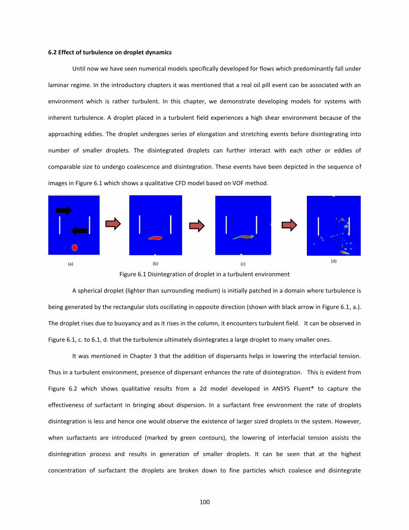
100

6.2 Effect of turbulence on droplet dynamics

Until now we have seen numerical models specifically developed for flows which predominantly fall under

laminar regime. In the introductory chapters it was mentioned that a real oil pill event can be associated with an

environment which is rather turbulent. In this chapter, we demonstrate developing models for systems with

inherent turbulence. A droplet placed in a turbulent field experiences a high shear environment because of the

approaching eddies. The droplet undergoes series of elongation and stretching events before disintegrating into

number of smaller droplets. The disintegrated droplets can further interact with each other or eddies of

comparable size to undergo coalescence and disintegration. These events have been depicted in the sequence of

images in Figure 6.1 which shows a qualitative CFD model based on VOF method.

Figure 6.1 Disintegration of droplet in a turbulent environment

A spherical droplet (lighter than surrounding medium) is initially patched in a domain where turbulence is

being generated by the rectangular slots oscillating in opposite direction (shown with black arrow in Figure 6.1, a.).

The droplet rises due to buoyancy and as it rises in the column, it encounters turbulent field. It can be observed in

Figure 6.1, c. to 6.1, d. that the turbulence ultimately disintegrates a large droplet to many smaller ones.

It was mentioned in Chapter 3 that the addition of dispersants helps in lowering the interfacial tension.

Thus in a turbulent environment, presence of dispersant enhances the rate of disintegration. This is evident from

Figure 6.2 which shows qualitative results from a 2d model developed in ANSYS Fluent® to capture the

effectiveness of surfactant in bringing about dispersion. In a surfactant free environment the rate of droplets

disintegration is less and hence one would observe the existence of larger sized droplets in the system. However,

when surfactants are introduced (marked by green contours), the lowering of interfacial tension assists the

disintegration process and results in generation of smaller droplets. It can be seen that at the highest

concentration of surfactant the droplets are broken down to fine particles which coalesce and disintegrate

(a) (b) (c)(d)

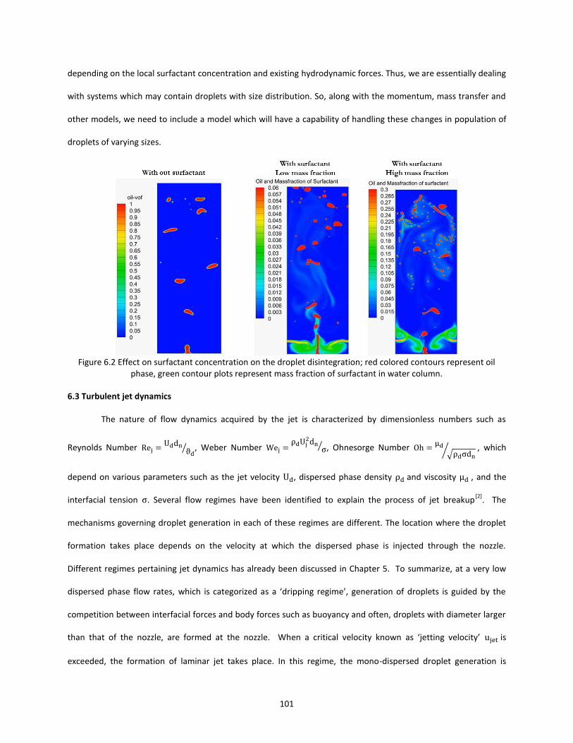
101

depending on the local surfactant concentration and existing hydrodynamic forces. Thus, we are essentially dealing

with systems which may contain droplets with size distribution. So, along with the momentum, mass transfer and

other models, we need to include a model which will have a capability of handling these changes in population of

droplets of varying sizes.

Figure 6.2 Effect on surfactant concentration on the droplet disintegration; red colored contours represent oil

phase, green contour plots represent mass fraction of surfactant in water column.

6.3 Turbulent jet dynamics

The nature of flow dynamics acquired by the jet is characterized by dimensionless numbers such as

Reynolds Number

⁄ , Weber Number

⁄ , Ohnesorge Number √ ⁄ , which

depend on various parameters such as the jet velocity , dispersed phase density and viscosity , and the

interfacial tension . Several flow regimes have been identified to explain the process of jet breakup[2]

. The

mechanisms governing droplet generation in each of these regimes are different. The location where the droplet

formation takes place depends on the velocity at which the dispersed phase is injected through the nozzle.

Different regimes pertaining jet dynamics has already been discussed in Chapter 5. To summarize, at a very low

dispersed phase flow rates, which is categorized as a ‘dripping regime’, generation of droplets is guided by the

competition between interfacial forces and body forces such as buoyancy and often, droplets with diameter larger

than that of the nozzle, are formed at the nozzle. hen a critical velocity known as ‘jetting velocity’ is

exceeded, the formation of laminar jet takes place. In this regime, the mono-dispersed droplet generation is

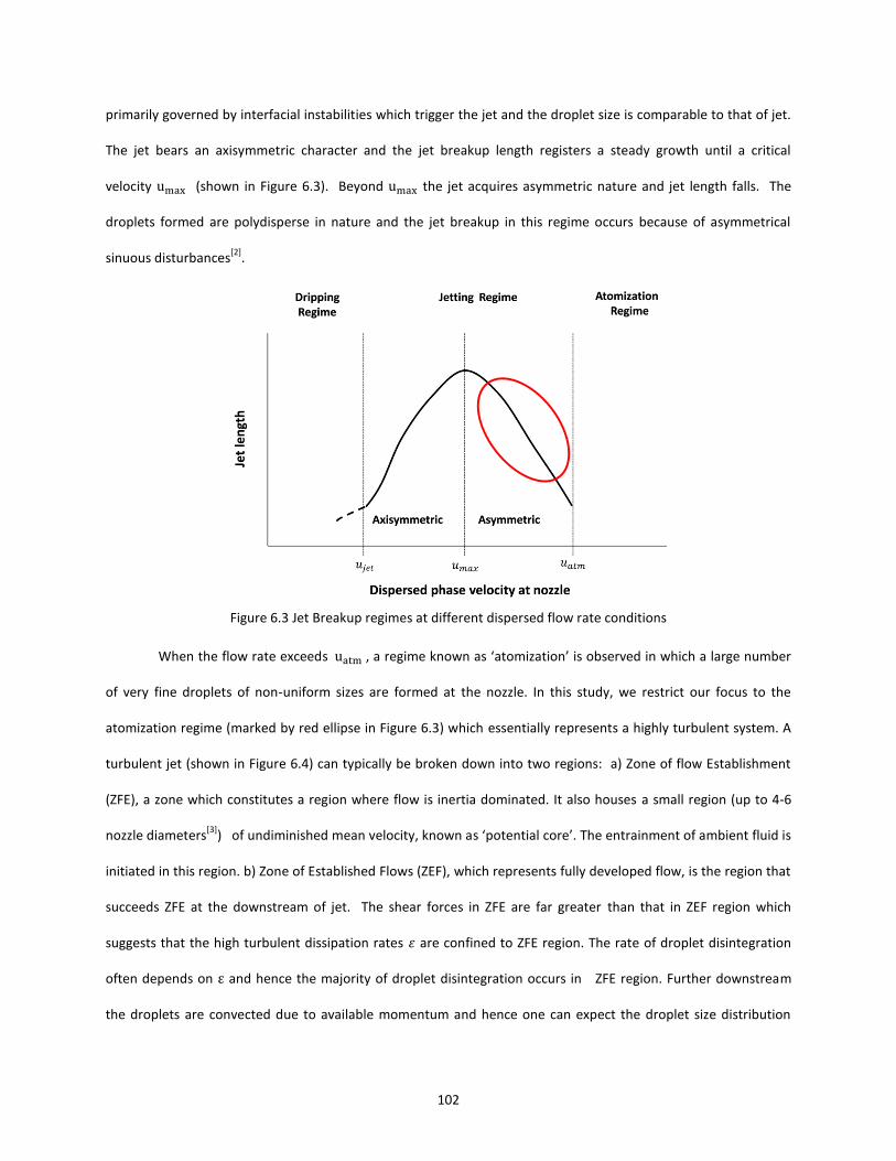
102

primarily governed by interfacial instabilities which trigger the jet and the droplet size is comparable to that of jet.

The jet bears an axisymmetric character and the jet breakup length registers a steady growth until a critical

velocity (shown in Figure 6.3). Beyond the jet acquires asymmetric nature and jet length falls. The

droplets formed are polydisperse in nature and the jet breakup in this regime occurs because of asymmetrical

sinuous disturbances[2]

.

Figure 6.3 Jet Breakup regimes at different dispersed flow rate conditions

When the flow rate exceeds , a regime known as ‘atomization’ is observed in which a large number

of very fine droplets of non-uniform sizes are formed at the nozzle. In this study, we restrict our focus to the

atomization regime (marked by red ellipse in Figure 6.3) which essentially represents a highly turbulent system. A

turbulent jet (shown in Figure 6.4) can typically be broken down into two regions: a) Zone of flow Establishment

(ZFE), a zone which constitutes a region where flow is inertia dominated. It also houses a small region (up to 4-6

nozzle diameters[3]

) of undiminished mean velocity, known as ‘potential core’. The entrainment of ambient fluid is

initiated in this region. b) Zone of Established Flows (ZEF), which represents fully developed flow, is the region that

succeeds ZFE at the downstream of jet. The shear forces in ZFE are far greater than that in ZEF region which

suggests that the high turbulent dissipation rates are confined to ZFE region. The rate of droplet disintegration

often depends on and hence the majority of droplet disintegration occurs in ZFE region. Further downstream

the droplets are convected due to available momentum and hence one can expect the droplet size distribution

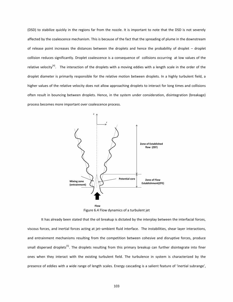
103

(DSD) to stabilize quickly in the regions far from the nozzle. It is important to note that the DSD is not severely

affected by the coalescence mechanism. This is because of the fact that the spreading of plume in the downstream

of release point increases the distances between the droplets and hence the probability of droplet – droplet

collision reduces significantly. Droplet coalescence is a consequence of collisions occurring at low values of the

relative velocity[4]

. The interaction of the droplets with a moving eddies with a length scale in the order of the

droplet diameter is primarily responsible for the relative motion between droplets. In a highly turbulent field, a

higher values of the relative velocity does not allow approaching droplets to interact for long times and collisions

often result in bouncing between droplets. Hence, in the system under consideration, disintegration (breakage)

process becomes more important over coalescence process.

Figure 6.4 Flow dynamics of a turbulent jet

It has already been stated that the oil breakup is dictated by the interplay between the interfacial forces,

viscous forces, and inertial forces acting at jet–ambient fluid interface. The instabilities, shear layer interactions,

and entrainment mechanisms resulting from the competition between cohesive and disruptive forces, produce

small dispersed droplets[5]

. The droplets resulting from this primary breakup can further disintegrate into finer

ones when they interact with the existing turbulent field. The turbulence in system is characterized by the

presence of eddies with a wide range of length scales. Energy cascading is a salient feature of ‘inertial subrange’,

Potential core

Flow

Mixing zone (entrainment)

Zone of Established flow (ZEF)

Zone of Flow Establishment(ZFE)

r

z

104

the regime where the inertial stresses dominate over viscous stresses. The kinetic energy is transferred from large

eddies to progressively smaller and smaller eddies. Most of the kinetic energy is believed to be contained in large

scale eddies and viscous forces do not have much role to play in large scale motion. However, at the smallest

scales (Kolmogorov scales), the viscous effects are dominant (viscous subrange) and eddies lose their energy

through viscous dissipation. The velocity fluctuations in a turbulent flow field thus, are a consequence of arrival of

eddies with spectrum of length scales[6]

. Eddies larger than the size of droplets assist in its bulk transportation. The

actual disintegration of droplet is brought in by the eddies of comparable size which has enough energy to

overcome the surface energy of the droplet[7]

. The collision of the arriving eddy imparts velocity fluctuations on the

surface of the droplet. The breakup of droplet is dictated by the balance of external stresses from the continuous

phase that tries to deform the droplet and surface stresses along with the viscous stresses inside the droplet that

have stabilizing effect and attempt to restore its form. Thus, disintegration occurs when amplitude of oscillations

are sufficiently large to allow droplet to deform and stretch itself leading to necking.

The concept of maximum stable droplet size in a turbulent field was proposed by Hinze[8]

, where an

analysis based on the forces controlling the deformation and the breakup of the droplet was presented to

calculate it. The breakup was deemed to occur when the local exceeded a critical Weber number[9]

which is ratio of shear forces to surface tension forces, given by

(6.1)

where is fluctuating velocity

[10] (valid for isotropic turbulence) defined as

( ) , is continuous

phase turbulent dissipation rate, is eddy length scale . The droplet is stable below and beyond it the

droplet breaks up. In the inertial subrange, the maximum stable diameter holds the relation[8]

(

)

(6.2)

It should be noted that in the present case, the droplets are continuously being transported to region of

lower and hence the disintegration would take place only if the droplet residence time in region with high is

greater than the breakup time . The droplet break up time in a turbulent field satisfies the relation[9]

,

(6.3)

105

This aspect would be discussed in greater detail in the later sections of this paper. The above parameters have

been shown in Figure 6.5.

Figure 6.5 Droplet disintegration process in a turbulent field (taken from Kolev

[11])

6.4 Numerical modelling

In this study, we present a numerical model for predicting the droplet size distribution resulting from the

interaction of turbulent oil jets with the surrounding quiescent environment. We achieve this objective by

integrating traditional multiphase CFD models with a population balance approach. The model thus developed is

composed of following components:

Multiphase model

Turbulence model

Population Balance model

Before considering the integrated model, a brief discussion on each of these models would be presented in

the following sections.

6.4.1 Multiphase Models

The interaction of oil (dispersed phase) with water which constitutes the continuous phase, necessitates

the inclusion of model to account for the multiphase nature of the problem. In earlier chapters we have

demonstrated the implementation of fully resolved model such as VOF for simulating the droplet motion in

quiescent environment. Employing interface tracking methods like VOF for simulating system containing large

number of droplets would be expensive computationally and hence not feasible. The two most popular

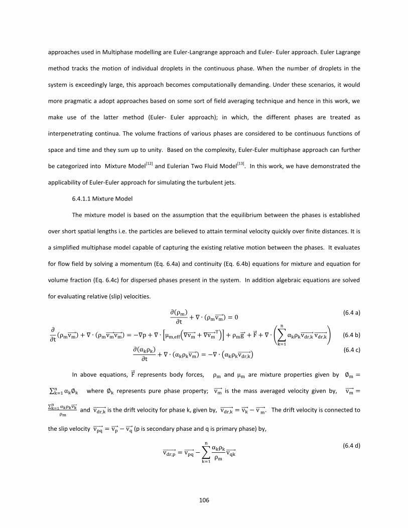
106

approaches used in Multiphase modelling are Euler-Langrange approach and Euler- Euler approach. Euler Lagrange

method tracks the motion of individual droplets in the continuous phase. When the number of droplets in the

system is exceedingly large, this approach becomes computationally demanding. Under these scenarios, it would

more pragmatic a adopt approaches based on some sort of field averaging technique and hence in this work, we

make use of the latter method (Euler- Euler approach); in which, the different phases are treated as

interpenetrating continua. The volume fractions of various phases are considered to be continuous functions of

space and time and they sum up to unity. Based on the complexity, Euler-Euler multiphase approach can further

be categorized into Mixture Model[12]

and Eulerian Two Fluid Model[13]

. In this work, we have demonstrated the

applicability of Euler-Euler approach for simulating the turbulent jets.

6.4.1.1 Mixture Model

The mixture model is based on the assumption that the equilibrium between the phases is established

over short spatial lengths i.e. the particles are believed to attain terminal velocity quickly over finite distances. It is

a simplified multiphase model capable of capturing the existing relative motion between the phases. It evaluates

for flow field by solving a momentum (Eq. 6.4a) and continuity (Eq. 6.4b) equations for mixture and equation for

volume fraction (Eq. 6.4c) for dispersed phases present in the system. In addition algebraic equations are solved

for evaluating relative (slip) velocities.

( )

( )

(6.4 a)

( ) ( ) [ (

)] (∑

) (6.4 b)

( )

( ) ( )

(6.4 c)

In above equations, represents body forces, and are mixture properties given by

∑ where represents pure phase property; is the mass averaged velocity given by,

∑

and is the drift velocity for phase k, given by, . The drift velocity is connected to

the slip velocity (p is secondary phase and q is primary phase) by,

∑

(6.4 d)

107

The slip velocity is calculated by the algebraic slip formulation described in Manninen et. al [14]

,

( )

( ( )

)

(

)

(6.4 e)

The presence of dispersed phase allows it to interact with the turbulent field and consequently there can

be some dispersion[15]

. The second term on RHS in Eq. 6.4e accounts for this; is the mixture turbulent viscosity

and is Prandtl dispersion coefficient and is the drag function which depends on the closure model for drag

force. The drag function is based on formulation suggested by Schiller and Naumann[16]

.

{

(6.4 f)

6.4.1.2 Eulerian Model

The Eulerian Two Fluid Model offers a more rigorous solution strategy for the flow field evaluation, in

the sense that the dedicated sets of continuity and momentum equations for each of the phases are solved. For a

phase ‘q’ the conservation of mass equation is

( )

( )

(6.5 a)

The momentum equation for each phase is given by,

( ) ( ) [ (

)]

(6.5 b)

where interphase force term is expressed as,

(6.5 c)

represent drag[16, 17]

, lift[13]

, virtual mass[13]

and turbulent dispersion forces respectively. The

momentum exchange terms are accounted for in .Drag force originates from the resistance experienced by the

dispersed phase moving in the continuous phase and is given by,

| |( )

(6.5 d)

where and are the continuous and dispersed phase velocities. , the drag coefficient is defined according to

the model suggested by Schiller and Naumann[16]

. The virtual mass force is caused by the relative acceleration

between the phases and is important when the dispersed phase density is much lesser than that of continuous

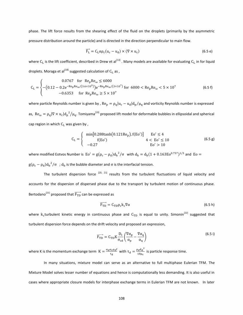
108

phase. The lift force results from the shearing effect of the fluid on the droplets (primarily by the asymmetric

pressure distribution around the particle) and is directed in the direction perpendicular to main flow.

( ) ( ) (6.5 e)

where is the lift coefficient, described in Drew et al[13]

. Many models are available for evaluating in for liquid

droplets. Moraga et al[18]

suggested calculation of as ,

{

( ( )) (

)

(6.5 f)

where particle Reynolds number is given by , | | ⁄ and vorticity Reynolds number is expressed

as, | | ⁄ . Tomiyama

[19] proposed lift model for deformable bubbles in ellipsoidal and spherical

cap region in which was given by ,

{ [ ( ) (

)]

( )

(6.5 g)

where modified Eotvos Number is ( ) ⁄ with (

) and

( ) ⁄ ; is the bubble diameter and is the interfacial tension.

The turbulent dispersion force [20, 21]

results from the turbulent fluctuations of liquid velocity and

accounts for the dispersion of dispersed phase due to the transport by turbulent motion of continuous phase.

Bertodano[21]

proposed that can be expressed as

(6.5 h)

where turbulent kinetic energy in continuous phase and is equal to unity. Simonin[22]

suggested that

turbulent dispersion force depends on the drift velocity and proposed an expression,

(

)

(6.5 i)

where K is the momentum exchange term

with

is particle response time.

In many situations, mixture model can serve as an alternative to full multiphase Eulerian TFM. The

Mixture Model solves lesser number of equations and hence is computationally less demanding. It is also useful in

cases where appropriate closure models for interphase exchange terms in Eulerian TFM are not known. In later

109

section, we present a case which demonstrates that the flow fields evaluated by either of these models are close

and so are the resulting overall size distributions of droplets.

6.4.2 Turbulence Models

It has been mentioned earlier that the turbulence plays an important in the system under consideration

and hence it governs the dynamics of oil droplets. So, it is essential to model turbulence to depict its effect on

droplet coalescence and disintegration. Turbulence represents a flow regime which is random and chaotic. It gives

rise to eddies of different length scales. The large eddies extract energy from the mean flow by the process of

‘vortex stretching’. Inertia dominates the large scale flows in a turbulent environment. The process of transfer of

the kinetic energy from large eddies to smaller eddies is termed as ‘energy cascade’. Cascading phenomenon has

been shown in Figure 6.6 which depicts the energy spectrum across eddies with different length scales. The lower

wavenumber represents larger eddies. The small scale motion in a turbulent field is equally dominated by inertia

and viscous effects. The smallest scales that exist are often termed as Kolmogorov scales. The energy associated

with these small structures is lost in form of heat through viscous dissipation. The larger eddies in a turbulent flow

are anisotropic whereas significantly small eddies bear an isotropic nature due to the diffusive action of viscosity.

Figure 6.6 Energy spectrum in a turbulent field (taken from

[23])

Many approaches are available for modelling turbulence existing in the flow field. Few have been

described briefly in the following section.

110

6.4.2.1 Reynolds Averaged Navier Stokes equation (RANS)

RANS analyzes the overall effect of turbulence on the mean flow properties. In traditional RANS approach,

the solution variables in instantaneous Navier Stokes equations are decomposed into mean and fluctuating

components. For instance, the instantaneous velocity can be expressed as,

(6.6)

where is the mean velocity and is the fluctuating component. The time averaging of NSE yields Reynolds

stress terms which are expressed as;

; ; ; ; (6.7)

These above terms are evaluated through closure models. Few methods used for modeling these are k- ε

,k-ω and Reynolds Stress model. The standard k- ε assumes that the turbulence to be isotropic and is one of the

popular turbulence models used by the industry. It solves dedicated transport equations for ‘k’, the turbulent

kinetic energy and the ‘ε’, the turbulent kinetic energy dissipation rate. The eddy viscosity is defined as ,

(6.8)

( )

( ) ((

) )

(6.9)

( )

( ) ((

) )

(6.10)

In above equations

[

] is the mean value of the rate of deformation of a fluid element in a

turbulent flow. The last two terms in Eq. 6.9 and 6.10 represent the rate of production and destruction of k and ε

respectively. There were flow situations to which standard k-ε cannot be applied. Improvements were brought to

standard k- ε model, to yield models such as RNG k- ε and Realizable k- ε model to increase its applicability. These

will be discussed later in the chapter.

The anisotropic nature of turbulent stresses is accounted for in Reynolds Stress Model. It is the most

elaborate RANS model available where the transport equations for Reynolds stresses along with the one for

dissipation rate are solved. In all seven additional transport equations are solved RSM which makes it

computationally more expensive.

111

6.4.2.2 Filtered Navier Stokes Equations (LES)

It has been mentioned that the behavior of large eddies is very different from the smaller eddies. Small

scale eddies are isotropic in nature. RANS models often do not differentiate between the large eddies and small

eddies and the effect of all eddies are described by a single turbulence model. The problem is more smartly

negotiated in LES method where all large scale eddies are resolved and the modelling is applied only to small scale

eddies. In this approach, the turbulent flow structure is resolved into distinct transport of large and small scale

motions by use of spatial filter functions. During spatial filtering the information related to the small scale eddies is

lost and interaction between the resolved and unresolved eddies gives rise to sub grid scale stresses which are

closed with the help of a model. Capturing transient structures inherent to turbulent flows is possible to time

dependent simulations based on LES. When compared to RANS methods, LES is more rigorous and hence

computationally more intensive.

6.4.3 Population Balance Models

It has been described that in the system under consideration droplets interact with each other and as well

as with turbulent field. In process they may undergo series of coalescence and disintegration which changes

number density of different sized droplets. The local droplet size distributions can be calculated by solving the

population balance equations[24]

. Population balance equation describes the temporal evolution of number

density function for particles by accounting for changes in population of particular sized particles, in a control

volume, due to convective transport, growth, coalescence and disintegration. A transport equation is written for

number density probability function ( ) of droplets, which is often related to internal coordinate[25]

such as

volume of droplet ‘V’.

[ ( )] [ ( )] [ ( )]

(6.11)

The second term represents the convective term; third term accounts for the growth process. In the

terms on RHS, superscripts ‘d’ and ‘c’ stand for the disintegration (sink) and coalescence (source) processes which

may result in birth and death of particle with size V. The birth and death terms are expressed as follows:

∫ ( ) ( ) ( )

(6.12)

∫ ( ) ( ) ( )

(6.13)

112

( ) ∫ ( )

( ) ( ) (6.14)

( ) ( ) (6.15)

Eq. (6.12), accounts for the generation of droplets with volume V due to coalescence between droplets of volume

and whereas in Eq. (6.13) represents the birth rate due to disintegration of larger droplets which yield

droplets with volume V. ( ) is the probability density of daughter droplets which represents the probability of

production of droplets with volume from breakage of droplets with size . The disappearance rate of volume

droplets due to coalesce with droplets V’ is expressed by Eq ( .14). Equation (6.15) gives the death rate expression

due to disintegration of droplets V. All the above expressions are required to be closed by an appropriate

disintegration and coalescence kernel functions, represented by and respectively. These are defined in

accordance to the various coalescence[26-29]

and disintegration[7, 26, 30]

mechanisms proposed in literature. Wang et.

al. [31]

have shown comparison of various coalescence and breakage kernels . The kernels encompass several

parameters which depend on operating conditions. The kernels included in a model would yield a reasonable DSD

only if it has been developed for situations which are closely related to the flow dynamics encountered in the

system under consideration. In following sections we have included a brief discussion on the coalescence and

breakage kernels.

6.4.3.1 Breakage / Disintegration models

The breakage mechanism (Figure 6.7) can be succinctly described by the balance between external

stresses exerted by the continuous phase which try to deform the droplet and viscous stresses of the fluid inside

the droplet that tend to restore its original shape. The disintegration of the droplet/bubble primarily occurs due to

one or the combination of the following;

presence of turbulent pressure fluctuations;

collision with turbulent eddy or turbulent shearing;

Viscous shear force;

Interfacial instability;

Shearing off process.

113

The breakage kernel accounting for the disintegration of the droplets in presence of turbulence has been

discussed in Luo et al[7]

which is based on the consideration of kinetic gas theory. The breakage rate is generally

expressed as

( ) ( ) ( | ) (6.16)

where refers to the volume of the parent droplet and disintegrated droplets bear a volume . ( ) is the

breakage frequency and ( | ) is the normalized daughter particle distribution function which is 0.5 for a binary

breakage. The model has been developed based on the assumption that the turbulence is isotropic. The breakup

rate is given by

( ) ∫

( )

( ) (6.17)

In above expression, refers to dimensionless eddy size which ratio of eddy size to diameter of

the droplet in the sub- inertial range . and b are parameters given by ;

[

( )

]

⁄ ;

;

where is the rate of energy dissipation per unit

mass. The numerator in Eq. 6.17 represents the ratio of the increased surface area of daughter droplets w.r.t

surface area of the parent droplet.

Another breakage kernel proposed by Martinez-Bazan et al[32]

is based on the fact that the probability of

breakup depends on the magnitude of the difference between the pressure gradient produced by the turbulent

fluctuations on droplet surface and the restoring pressure by surface tension.

( )

√

( )

(6.18)

where is turbulent velocity.

Figure 6.7 Breakage mechanism a) Luo and Svendson

[7] b) Martinez- Bazan et.al

[32] (taken from Chen

[28])

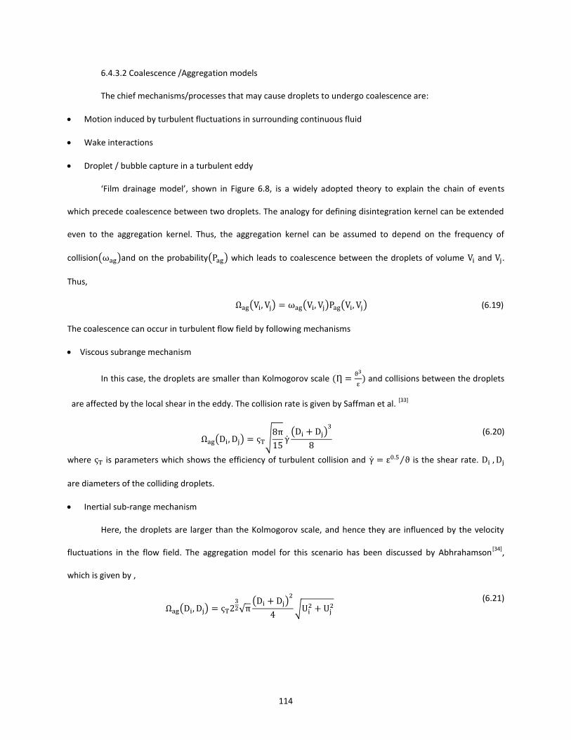
114

6.4.3.2 Coalescence /Aggregation models

The chief mechanisms/processes that may cause droplets to undergo coalescence are:

Motion induced by turbulent fluctuations in surrounding continuous fluid

Wake interactions

Droplet / bubble capture in a turbulent eddy

‘Film drainage model’, shown in Figure . , is a widely adopted theory to explain the chain of events

which precede coalescence between two droplets. The analogy for defining disintegration kernel can be extended

even to the aggregation kernel. Thus, the aggregation kernel can be assumed to depend on the frequency of

collision( )and on the probability( ) which leads to coalescence between the droplets of volume and .

Thus,

( ) ( ) ( ) (6.19)

The coalescence can occur in turbulent flow field by following mechanisms

Viscous subrange mechanism

In this case, the droplets are smaller than Kolmogorov scale (

) and collisions between the droplets

are affected by the local shear in the eddy. The collision rate is given by Saffman et al. [33]

( ) √

( )

(6.20)

where is parameters which shows the efficiency of turbulent collision and ⁄ is the shear rate.

are diameters of the colliding droplets.

Inertial sub-range mechanism

Here, the droplets are larger than the Kolmogorov scale, and hence they are influenced by the velocity

fluctuations in the flow field. The aggregation model for this scenario has been discussed by Abhrahamson[34]

,

which is given by ,

( ) √

( )

√

(6.21)

115

where and

are the mean squared velocities for droplets ‘i’ and ‘j’ respectively. (

)

; is

ration between the viscous force and Van der waals force given by ( ) ⁄ where H is Hamaker

constant which depends on the material of particle(bubble/droplet) which is being deformed.

Prince et al[35]

in their work have proposed coalescence rate considering the turbulent collision which is

expressed as ,

( )

( )

√

(

)

(6.22)

where is calibration factor for coalescence , is time required for bubbles of diameters and to coalesce,

is the contact time for two bubbles.

Figure 6.8 Coalescence Mechanism in a turbulent flow (taken from Chen

[28])

Many methods have been discussed in literature for solving PBE (Eq. 6.11); the chief ones being , Monte

Carlo Method[36, 37]

, Method of Moments [38-40]

and Method of classes[24, 41, 42]

. In this work, we follow method of

classes for discretizing of PBE, in which a continuous particle size distribution is represented in terms of set of

discrete classes/bins. The bins are defined as

(6.23)

where is the discretization factor and is the bin with the minimum sized particles , is number of classes.

For each of the classes following equation is formulated,

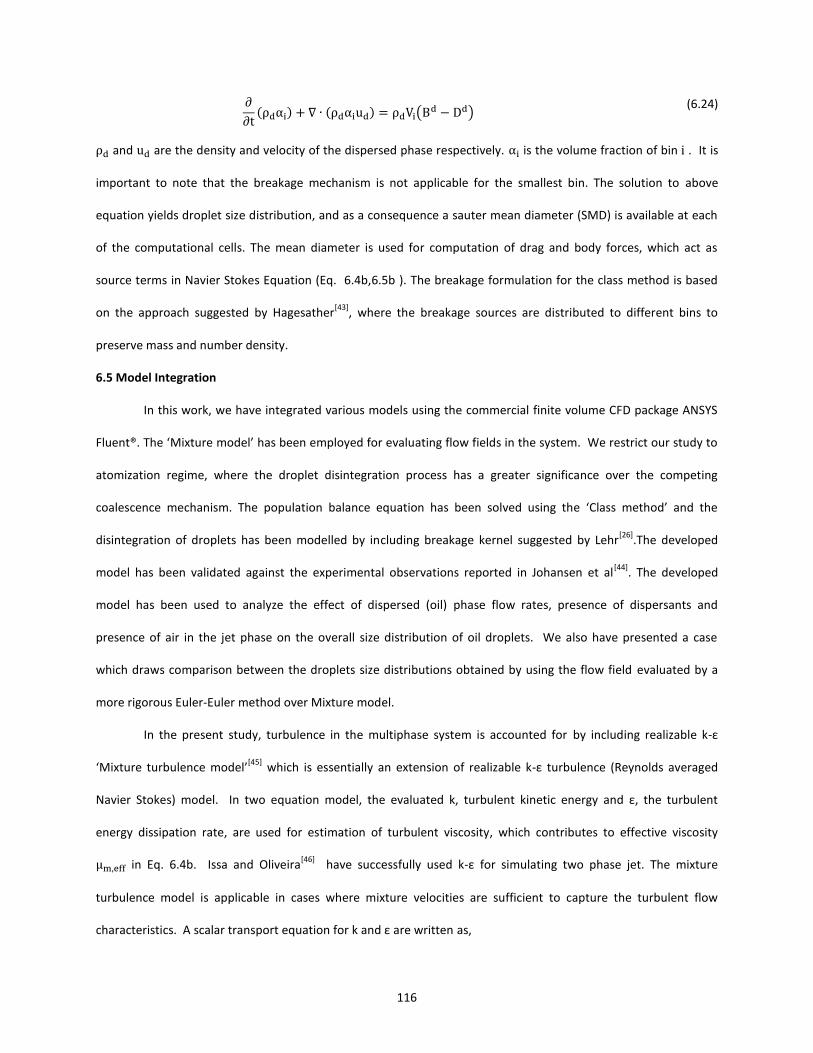
116

( ) ( ) (

) (6.24)

and are the density and velocity of the dispersed phase respectively. is the volume fraction of bin . It is

important to note that the breakage mechanism is not applicable for the smallest bin. The solution to above

equation yields droplet size distribution, and as a consequence a sauter mean diameter (SMD) is available at each

of the computational cells. The mean diameter is used for computation of drag and body forces, which act as

source terms in Navier Stokes Equation (Eq. 6.4b,6.5b ). The breakage formulation for the class method is based

on the approach suggested by Hagesather[43]

, where the breakage sources are distributed to different bins to

preserve mass and number density.

6.5 Model Integration

In this work, we have integrated various models using the commercial finite volume CFD package ANSYS

Fluent®. The ‘ ixture model’ has been employed for evaluating flow fields in the system. e restrict our study to

atomization regime, where the droplet disintegration process has a greater significance over the competing

coalescence mechanism. The population balance equation has been solved using the ‘Class method’ and the

disintegration of droplets has been modelled by including breakage kernel suggested by Lehr[26]

.The developed

model has been validated against the experimental observations reported in Johansen et al[44]

. The developed

model has been used to analyze the effect of dispersed (oil) phase flow rates, presence of dispersants and

presence of air in the jet phase on the overall size distribution of oil droplets. We also have presented a case

which draws comparison between the droplets size distributions obtained by using the flow field evaluated by a

more rigorous Euler-Euler method over Mixture model.

In the present study, turbulence in the multiphase system is accounted for by including realizable k-ε

‘ ixture turbulence model’[45]

which is essentially an extension of realizable k-ε turbulence (Reynolds averaged

Navier Stokes) model. In two equation model, the evaluated k, turbulent kinetic energy and ε, the turbulent

energy dissipation rate, are used for estimation of turbulent viscosity, which contributes to effective viscosity

in Eq. 6.4b. Issa and Oliveira[46]

have successfully used k-ε for simulating two phase jet. The mixture

turbulence model is applicable in cases where mixture velocities are sufficient to capture the turbulent flow

characteristics. A scalar transport equation for k and ε are written as,

117

( )

( ) ((

) ) (6.25 a)

( )

( ) ((

) )

√

(6.25 b)

where =max[

] with

. The last two terms in above equations represent the generation and

destruction of k and . The turbulent viscosity is given by

. The generation of k is included in

which is given by ( ) . Further, standard values were used for all constants

( =1 ; =1.2; =1.44 ; =1.9).

In the cases where Euler Two Fluid Model is employed we make use of a more involved k-ε ‘Per phase

turbulence model’, in which k and ε equations are formulated for each of the phases. For q phase the weighted

transport of k and are written as,

( )

( )

((

) )

∑ ( ) ∑ ( )

∑ ( )

(6.26 a)

( )

( )

((

) ) (

√ )

[ (∑ ( ) ∑ ( )

∑ ( )

)]

(6.26 b)

In above equations, =2 , (

⁄

⁄) with and being characteristic particle

relaxation time and Lagrangian integral time[47]

respectively. represent interphase momentum exchange

coefficient given by ⁄ , with

⁄ .

It has been mentioned in previous sections, that in present case, disintegration process is dominant and

has greater influence on droplet size distribution. In the integrated model development, we account for the

118

droplet breakage by including the breakage kernel proposed by Lehr[26]

. This breakage kernel has been developed

with an assumption the disintegration of the droplet occurs when eddies smaller than the length scales of droplet

collide with it, resulting in generation of two droplets (binary breakage). The breakup is determined by the balance

between the interfacial tension force of the droplet and the inertial force of the approaching eddy. The breakage

kernel function in general bears the form,

( ) ( ) ( ) (6.27 a)

where ( ) is breakup frequency and ( ) denotes the normalized daughter size distribution function. Lehr

model is an integrated kernel in the sense that it includes both breakup frequency and daughter size distribution. It

is given by,

( ) ∫

( )

⁄

( ( )⁄ ) (6.27 b)

with ⁄ ⁄

⁄⁄ ;

⁄

⁄ ⁄⁄ and ⁄ .

In these expressions, = Eddy size, = droplet size, = Critical Weber Number f= Breakage volume

fraction = Minimum eddy size in inertial sub range. The kernel is valid in the inertial subrange of turbulence

which is isotropic in nature. Eq. 6.26b indicates the dependence of breakage kernel on the turbulence dissipation

rates ε interfacial tension and droplet diameter d.

The integrated model is shown in Figure 6.9 which depicts the interaction among models discussed in

preceding sections. It can be seen that all the models are intricately coupled to each other. The solution of

continuity and NSE helps in evaluating the velocity field. The appearing in NSE is obtained from the k-ε

turbulence model, which makes use of velocity field for solving convective tern in k and ε transport equations. In

each of the computational cells, the term accounting for body forces in the momentum equation is evaluated by

considering the sauter mean diameter obtained from the coupling established between the population balance

model with CFD. The disintegration rate in the dispersed phase is calculated by employing the invoked breakage

kernel.

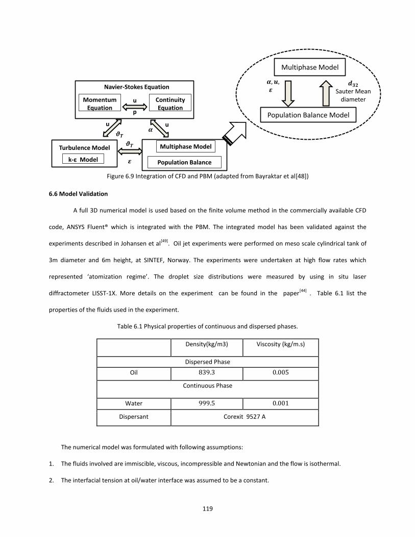
119

Figure 6.9 Integration of CFD and PBM (adapted from Bayraktar et al[48])

6.6 Model Validation

A full 3D numerical model is used based on the finite volume method in the commercially available CFD

code, ANSYS Fluent® which is integrated with the PBM. The integrated model has been validated against the

experiments described in Johansen et al[49]

. Oil jet experiments were performed on meso scale cylindrical tank of

3m diameter and 6m height, at SINTEF, Norway. The experiments were undertaken at high flow rates which

represented ‘atomization regime’. The droplet size distributions were measured by using in situ laser

diffractometer LISST-1X. More details on the experiment can be found in the paper[44]

. Table 6.1 list the

properties of the fluids used in the experiment.

Table 6.1 Physical properties of continuous and dispersed phases.

Density(kg/m3) Viscosity (kg/m.s)

Dispersed Phase

Oil

Continuous Phase

Water

Dispersant Corexit 9527 A

The numerical model was formulated with following assumptions:

1. The fluids involved are immiscible, viscous, incompressible and Newtonian and the flow is isothermal.

2. The interfacial tension at oil/water interface was assumed to be a constant.

Navier-Stokes Equation

Momentum Equation

Continuity Equation

u

p

Turbulence Model

k-ε Model

u

u

Multiphase Model

Population Balance

Multiphase Model

Population Balance Model

Sauter Mean

diameter

120

3. The turbulence in the system is isotropic.

4. The operating conditions in the system allow for breakup to be the dominant process.

6.6.1 Computational domain and Boundary conditions

It has been mentioned earlier that the droplet disintegration is relevant only in regions (near the nozzle)

where turbulence is high. Hence, the numerical investigation is carried out on a cylindrical domain with diameter

equal to 200 times the nozzle diameter and around 350 nozzle diameters in height. The transient simulation was

carried out using second order implicit scheme. The pressure velocity coupling was established using SIMPLE[50]

(Semi-Implicit Method for Pressure-Linked Equations) scheme. The second order upwind differencing scheme was

used for spatial discretization in momentum, volume fraction, k, ε and population balance equations. The

calculation of gradients was based on the Green-Gauss Cell Based method. PRESTO (Pressure Staggering Option)

scheme was employed for pressure interpolation. The computational domain for simulation along with the

boundary conditions has been shown in Figure 6.10. A structured meshing was built over the domain using ANSYS

ICEM.

Figure 6.10 Computational domain and boundary conditions

h=0

.5m

d=0.3m

nozzle

Outer boundary(symmetry)

Top (Outlet)

Jet inlet (velocity inlet)

Floor (wall)

121

The wall boundary condition imposes no slip (all components of velocities are zero) at the lower face

(floor) of the computational domain.

(6.28 a)

The velocity inlet boundary condition is imposed at the jet inlet face, wherein the velocity corresponding

to the flow rate of dispersed phase is specified. Further, the value of k and ε are calculated on the basis of the

turbulent intensity (5%) specified at the inlet face. ne of the requirements of ‘class method’ for solving

Population Balance equation is the availability initial particle size distribution. The initial size distribution for

various droplet bins, in accordance to the experiment[49]

, is supplied at inlet. As breakage phenomenon is a

dominant process for the system another consideration, an initial DSD biased towards larger droplets is set at the

inlet.

Symmetric boundary conditions (terminology used in ANSYS Fluent®) are imposed at the periphery of

cylindrical computational domain, which ensures that at the normal component of velocities is zero and the

normal gradients of all other quantities are zero.

(6.28b)

At the top surface, pressure outlet boundary condition is applied and the zero flux condition is specified

for various bin fractions.

The simulation details used for validation have been enlisted in Table 6.2. The value of critical Weber

Number of 0.24 was used in the simulations. The simulations were performed with 32 processors on the

Supermike cluster of High Performance computing (HPC) facility located at Louisiana State University.

In this study, we have used the experimental observations conducted on a meso-scale apparatus at

SINTEF[49]

, for validating the integrated model. The agreement between the DSD predicted from the integrated

model, shown in Figure 6.11, a., is found to be satisfactory. In all of our simulations, DSD has been measured

across the horizontal plane across jet at an elevation of z=0.425m where the DSD could safely be assumed to have

stabilized. Figure 6.11, b. depicts the variation of turbulent dissipation rate along jet centerline. It can be seen

that decays exponentially to a low value (O(1)) within 100 nozzle diameters and hence disintegration of droplets

are restricted to this region. A similar trend can be noticed in Figure 6.11, d., which shows the variation of across

122

jet width at different heights. The size distribution can be thought to stabilize by the end of this region and the

beyond this point, droplets are merely convected due to available buoyancy.

Table 6.2 Simulation details for Model validation

Turbulence Model k-ε (RANS)

PBM Method Discrete Method

Number of bins 30

Minimum bin size (m)

Maximum bin size (m)

Breakage Kernel Lehr Model

Computational cells 201,000

Interfacial Tension (mN/m) 15.5

Oil flow rate (L/min) 1.5

Figure 6.11, e. shows the initial and final droplet size distributions .The final DSD does indirectly depend

on the local velocity field, volume fraction etc. and hence a good agreement with the DSD observed in the

experiment suggests that the model is able to predict the velocity field and the dispersed phase volume fraction

with a fair accuracy. Figure 6.11, c. reveals the velocity magnitude profiles of the mixture across the jet width at

different elevations along nozzle axis. The simulation result (Figure 6.11, f.) reveals that the velocity fields along

the jet width in the downstream of nozzle exhibit self-similarity. This is in congruence with the observations

reported for single phase turbulent jets in the literature[51]

and compares well with solution given for velocity

profiles by Tollmien[51]

.

The result for mesh sensitive test is shown in Figure 6.12. Simulations were carried for domain containing

20,000 , 112,000 , 201,000 and 300,500 elements. The variation of along the nozzle axis for domain has been

shown in Figure 6.12. It can be the value of predicted with mesh containing 201,000 tetrahedral elements are

similar to those found for mesh with 300,500 and hence the latter mesh resolution has been used for carrying out

rest of the simulations.

123

Figure .11 a) Comparison of DSD from model and experiment, b) Variation of ε along jet centreline, c) ixture velocity magnitude across jet width with z and d) Variation of ε across jet width along z e) Initial DSD at inlet and

final DSD at z=0.425m, f) Self similarity exhibited by velocity along z ; U is the velocity magnitude in radial direction , Um is velocity magnitude at the jet centerline, ‘b’ is the distance from the centerline in the radial direction ‘r’,

where the jet velocity equals 0.5Um

0

0.02

0.04

0.06

0.08

0.1

0.12

Bin

vo

lum

e f

ract

ion

Bin size (m)

CFD+PBM

Experiment

0.01

0.1

1

10

100

1000

10000

0 0.1 0.2 0.3 0.4 0.5

Tu

rbu

len

t d

issp

ati

on

ra

te (m

2/s

3)

Distance from nozzle (m)

0

2

4

6

8

10

12

14

16

-0.01 -0.005 0 0.005 0.01

Ve

loci

ty m

ag

nit

ud

e (

m/s

)

Jet width (m)

jet_inletz=0.005z=0.015z=0.025z=0.055z=0.225

0.00001

0.0001

0.001

0.01

0.1

1

10

100

1000

10000

-0.01 -0.005 0 0.005 0.01T

urb

ule

nt

dis

sip

ati

on

ra

te (

m2/s

3)

Jet width (m)

z=0.015

z=0.025

z=0.055

z=0.225

z=0.325

0

0.1

0.2

0.3

0.4

0.5

0.6

Bin

vo

lum

e f

ract

ion

Bin size (m)

Final DSD

initial DSD

0

0.2

0.4

0.6

0.8

1

1.2

0 0.5 1 1.5 2 2.5

U/U

m

r/b

z=0.005

z=0.015

z=0.025

z=0.035

z=0.045

z=0.055

z=0.065

z=0.125

z=0.225

Tollmien_solution

(e) (f)

(d)(c)

(b)(a)

124

Figure 6.12 Variation of turbulent dissipation rates averaged across the jet width with distance from nozzle

6.7 Mixture model v/s Eulerian Two Fluid Model

It has been discussed in earlier sections, that the disintegration of droplets is influenced by the local

turbulence. The droplet size distribution predicted by the model depends on the accuracy with which the

turbulent flow field is evaluated. In this section, we make an attempt to compare the flow fields resulting from

‘ ixture model’ with that from a more rigorous ‘Eulerian Two Fluid model’ and analyze their influence on the

overall DSD. The ‘ ixture turbulence model’ was coupled with ixture model, while ‘Per phase

turbulence model’ was used with Eulerian two fluid model for computing the turbulent flow fields. The comparison

between the two models has been show in Figure 6.13.

Simulations were carried on the computational domain described in previous sections. The flow rate of

dispersed phase was 1.5 L/min and the interfacial tension was kept at 15.5 mN/m. In each of these approaches

the drag was calculated using the formulation suggested by Schiller and Naumann [16]

. Since, the dispersed phase is

composed of fluid particles a drag factor of 0.75 was used in simulations. In the Eulerian two fluid model , lift

forces were computed from closure model proposed by Tomiyama[19]

. The turbulent dispersion force , which

represents turbulent diffusion in dispersed flows , is modeled by including a source term ( ) in phase

volume fraction equation (Eq. 5a) . represent the diffusion coefficient in ‘q’ phase given by

⁄ .

More details on this this can be found in work described in Sokolichin et al[20]

.

0.1

1

10

100

1000

10000

100000

0 0.05 0.1 0.15 0.2

Turb

ule

nt

dis

spat

ion

rat

e (

m2 /

s3 )

Distance from nozzle (m)

#22000

#112000

#201000

#305000

125

Figure 6.13 Comparison between Mixture model and Eulerian Two Fluid Model

Figure 6.13, a. shows that the velocity magnitude for oil phase averaged over jet width at different

elevations from the nozzle. It can be seen that the values predicted by the Mixture model is not very different than

that predicted by the computationally intensive Eulerian two fluid model. Further, a look at the plot of evaluated

turbulent dissipation rates shown in Figure 6.13, b. indicates that for the given case, the ‘ ixture turbulence

model’ is able to perform as well as the more seemingly rigorous ‘Per phase turbulence model’. The consequence

of these observations is reflected in DSD plot (Figure 6.13, c.) plot , which shows that a much simpler Mixture

model / Mixture turbulence model is capable of yielding a size distribution at par with that predicted from

Eulerian TFM/Per phase turbulence models. The mixture model employs algebraic slip formulation which is based

on the assumption that a local equilibrium between the phases is attained over small spatial length scale. The

calculated slip velocities depend on the drag and buoyancy force. A good agreement between the velocity fields

predicted by the Eulerian and Mixture models as highlighted before, indeed shows that, in these simulations, the

drag and buoyancy forces are more important than lift, turbulent dispersion and virtual mass forces (which are

0

0.02

0.04

0.06

0.08

0.1

0.12

Bin

vo

lum

e f

ract

ion

Bin size (m)

CFD+PBM_Mixture

CFD+PBM_TFM

0

0.00001

0.00002

0.00003

0.00004

0.00005

0.00006

0.00007

0.00008

0.00009

0.0001

0 0.1 0.2 0.3 0.4 0.5

Sau

ter

Me

an d

iam

ete

r (m

)

Distance from nozzle (m)

No dispersant _mixture

No dispersant_ TFM

0.01

0.1

1

10

100

1000

0 0.1 0.2 0.3 0.4 0.5

Turb

ule

nt

dis

spat

ion

rat

e (

m2 /

s3 )

Distance from nozzle (m)

No dispersant _mixture

No dispersant_ TFM

0

0.5

1

1.5

2

2.5

3

3.5

0 0.1 0.2 0.3 0.4 0.5

Ve

loci

ty m

agn

itu

de

oil

ph

ase

(m

/s)

Distance from nozzle (m)

No dispersant _mixture

No dispersant_ TFM

(a) (b)

(c) (d)

126

essentially included in the rigorous Eulerian model).This is attributed to the presence of the smaller sized droplets

in the system. The per-phase-turbulence-model is at best an ad-hoc extension to TFM framework and the

theoretical underpinnings of such extensions is still to be explored. Since the DSD is largely influenced by the

turbulence energy dissipation rate and the simpler single field turbulence model within the mixture framework

does an adequate job, it is deemed to be acceptable for parametric studies. For this reason, the former

combination of models is employed for carrying out rest of the simulations.

6.8 Results and discussion

Simulations were carried out for the computational domain described in earlier sections. Three different

scenarios were examined, where the parameters like, oil injection flow rates, interfacial tension and the buoyancy

of the dispersed phase played an important role in determination of the net droplet size distribution. The following

cases were studied;

Effect of varying oil injection rates on DSD,

Effect of dispersant concentration on DSD,

Effect of presence of gas phase on DSD.

In each of these studies, particle size range was discretized into 30 bins, which were evenly spaced on the

logarithmic scale. The disintegration process was not accounted for the droplets in the smallest bin.

6.8.1 Effect of dispersed phase flow rates on droplet size distribution

Investigations were carried out for three different dispersed phase flow rates, 0.5, 1.2 and 2.8 L/min,

corresponding to the dispersed phase Reynolds Numbers of 1200, 2845 and 6650 respectively. The interfacial

tension was kept constant at 15.5 mN/m. The results have been described in Figure 6.14. Figure 6.14, a. depicts

the DSD observed at z= 0.425m from nozzle, for different flow rates. It can be seen that at the higher flow rates,

size distribution curve shifts towards smaller bins, suggesting that degree of disintegration is relatively higher. This

fact can be confirmed from Figure 6.14, b., which shows Sauter mean diameter at different elevations. It can

be seen that for each of the flow rates, the values stabilizes within distances of 100 nozzle diameters from the

nozzle. The higher disintegration rates can be attributed be to the existence of high dissipation rates (shown in

Figure 6.15) in cases with larger dispersed phase flow rates.

127

Figure 6.14 a) Droplet size distribution at a distance z=0.425 from nozzle b) Sauter mean diameter averaged over horizontal planes across jet at different elevations

Figure 6.15 Averaged turbulence dissipation rates at oil injection flow rate 0.5 L/min, 1.2 L/min and 2.8 L/min.

6.8.2 Effect of dispersant concentration on droplet size distribution

During deep water oil spills dispersants are often added to disperse the larger oil droplets into finer

ones[52]

. In these scenarios, the concentrations are usually reported in terms of dispersant to oil ratio (DOR v/v %).

The effect of presence of dispersants has been studied by considering D R’s of 0 (dispersant free environment,

), 1:250 and 1:25. The operating conditions were similar to that described in Johansen et al[49]

. The injection

rate of the oil phase was kept constant at 1.5 L/min. In these studies, the transport of dispersant in the dispersed

and continuous phases has not been considered; rather we make an assumption that the IFT has a constant value

at the oil/ water interface, depending on the concentration of the dispersant. In reality of course, the strategies for

injection of the dispersant and its transport across the aqueous medium to the oleic phase are important issues to

0

0.02

0.04

0.06

0.08

0.1

0.12

Bin

vo

lum

r fr

acti

on

Bin size (m)

0.5 L/min

1.2 L/min

2.8 L/min

0

0.00001

0.00002

0.00003

0.00004

0.00005

0.00006

0.00007

0.00008

0.00009

0.0001

0 0.1 0.2 0.3 0.4 0.5

Sau

ter

Me

an d

iam

ete

r (m

)

Distance from nozzle (m)

0.5 L/min

1.2 L/min

2.8 L/min

(a) (b)

0.001

0.01

0.1

1

10

100

1000

10000

100000

1000000

0 0.1 0.2 0.3 0.4 0.5

Turb

ule

nt

dis

spat

ion

rat

e (

m2 /

s3 )

Distance from nozzle (m)

0.5 L/min

1.2 L/min

2.8 L/min

128

be addressed. The measured values IFT at various D R’s reported in ohansen et al[49]

were ultimately used in the

integrated model. The specifications of simulations are listed in Table 6.3.

Table 6.3 Simulation specifications for DSD prediction at different DOR's

DOR No dispersant 1: 250 1:25

IFT (mN/m) 15.5 2.6 0.05

Flow Rate (L/min) 1.5

Nozzle diameter (mm) 1.5

Figure 6.16, a. shows the net droplet size distributions at various D R’s. It can be observed that the mean

droplet size (Figure 6.16, b.) decreases with increase in dispersant concentration. As the flow rates are same in

each the case, the turbulence dissipation rate, along the jet, keeps a similar profile. However, increased

dispersant concentration leads to lowering of interfacial tension at the oil/water interface by a greater degree. It

has been mentioned earlier that the droplet disintegration is governed by the competition between the disruptive

inertial forces and the restoring surface tension forces. The reduction in the value of interfacial tension assists the

disintegration process and yields much smaller droplets. Thus, at higher dispersant concentrations, DSD shifts to

left.

Figure 6.16 Effect of dispersants on: a) droplet size distribution (z=0.425m), b) Sauter mean diameter across

vertical elevation

A glimpse at Figure 6.16, a. would reveal that the volume fraction of the smallest bin is abnormally high

for situations with high disintegration rate. This occurs because of the fact that the disintegration kernels exclude

No disp0

0.02

0.04

0.06

0.08

0.1

0.12

0.14

Bin

vo

lum

e f

ract

ion

Bin Size (m)

No disp

DOR 1:250

DOR 1:25

0

0.00001

0.00002

0.00003

0.00004

0.00005

0.00006

0.00007

0.00008

0.00009

0.0001

0 0.1 0.2 0.3 0.4 0.5

Sau

ter

Me

an d

iam

ete

r (m

)

Distance from nozzle (m)

No dispersant

DOR 1:250

DOR 1:25

(a) (b)

129

the breakup process for the lowest sized bins. Thus, the disintegration process propagates until the bin carrying

smallest of the droplets defined in the model and leads to the accumulation of droplets represented by the

smallest bin.

6.8.3 Effect of presence of gas phase on DSD

Oil and gas often coexist in nature due to high reservoir pressures and the plume associated with

subsurface releases can be treated as a mixture of oil and gas. The presence of gas phase acts as source of

buoyancy, which ultimately drives the plume. The typical gas to oil ratio observed during Deepwater Horizon

accident varied from 1500 to 2500 ft3/barrel oil (350 to 600 v/v%)

[53]. In this section, we present the results from

the CFD simulation, where the injected dispersed phase consists of the mixture of air and oil, with air to oil ratio of

10:1. Here, it is worthy to state that, the interaction between the air bubbles and oil droplets leading to droplet-

bubble coalescence and disintegration has been ignored as low probability events.

6.8.3.1 Constant dispersed phase flow rate

In the current set of simulations the overall volumetric flow rate through the inlet has been kept

constant. The air bubbles of diameter 40 m are introduced through the inlet with the same velocity as the oil jet.

The resulting droplet size distributions are compared with case where pure oil is introduced at same flow rate.

The dispersed phase flow rate and the interfacial tension used in the simulation are 1.5 L/min and 15.5 mN/m

respectively. The population balance equations are solved only for the oil phase and the gross effect of gas phase is

in imparting additional buoyancy to the oil phase. The mixture model allows for calculating the slip velocities

between continuous and dispersed phases through the approach suggested by Manninen et al[54]

.

It can be observed in Figure 6.17, a. that presence of air in the dispersed phase yields a droplet size

distribution which is biased towards larger bins, when compared to the case where pure oil jet is injected through

the nozzle. The reduction in disintegration rates can be explained by Figure 6.17, b., which indicates that the

dissipation rates in the near nozzle region is smaller than for the former case. This is observed because of the fact

that, a lot lesser momentum is available to the mixture of oil-air phase than that for pure oil phase injected at a

same flow rate.

130

Figure 6.17 Influence of gas phase injected at constant volumetric flow rate on a) Droplet size distribution of oil

droplets, b) turbulence energy dissipation rates

Further, the presence of air essentially imparts greater buoyancy to the plume. This can be confirmed

from Fig 6.18, which depicts the mixture density across plume width at different distances from the nozzle for the

dispersed phases with and without air and hence droplets are unable to spend long times in the region of higher

turbulence and hence do not witness a higher instances of disintegration.

Figure 6.18 Comparison of mixture density at different elevations for cases with or without air in dispersed phase

A more convincing explanation for the reduced disintegration can be built around concept of breakup

time ; which is the minimum time, a particular sized droplet has to be exposed in the turbulent field, to undergo

disintegration. The breakage time in a turbulent field, is approximately given by Eq. 6.3, which has dependency

on dissipation rates and the droplet diameter. Figure 6.19 uses the definition given in Eq. 6.3 to show the

breakage times at different distances for the droplets in the size range represented by the bins described in the

model. The plot basically depicts the minimum time required by droplets to breakup if they stay at the particular

elevation in the existing turbulent field. It can be inferred from Figure 6.19, a, b and c that the for case where

0.01

0.1

1

10

100

1000

10000

100000

0 0.1 0.2 0.3 0.4 0.5

Turb

ule

nt

Dis

spat

ion

Ene

rgy

(m2 /

s3 )

Distance from the nozzle (m)

Oil

Air-Oil 10:1

0

0.02

0.04

0.06

0.08

0.1

0.12

0.14

Bin

vo

lum

e f

ract

ion

Bin size (m)

Oil

Air-oil 10:1

(a) (b)

500

550

600

650

700

750

800

850

900

950

1000

0 0.1 0.2 0.3 0.4 0.5

Mix

ture

de

nsi

ty (

kg/m

3 )

Distance from the nozzle (m)

Oil

Air-Oil 10:1

131

dispersed phase is composed of air and oil, is greater than that in case where pure oil phase is injected . Thus, the

droplets in the former case undergo lesser degree of disintegration and are larger in size than that in latter case.

Figure 6.19 Comparison of breakage for dispersed phase with or without air at a) z=0.025m, b) z=0.125m and c)

z=0.325m

6.8.3.2 Constant dispersed phase Momentum

In this case the dispersed phase in either scenario is introduced from the inlet at a constant momentum

flux ( ). The air-oil mixture is injected and at flow rate of 1.5L/min and the corresponding flow rate for an oil jet

bearing equivalent momentum flux is 0.45 L/min. The results have been summarized in Figure 6.20. It can be seen

(Figure 6.20, a.) that the presence of air in the dispersed phase yields a DSD with smaller droplets. The SMD for this

case was found to be 30 m. However, for pure oil jet the resulting size distribution had a S D of 5 m. The

addition of gas at the inlet increases the local velocity gradients in both continuous and dispersed phases and

provides the system with an additional source of energy. Thus, the dissipation rates in the near nozzle region are

lot higher for case where air is present. This has been depicted in Figure 6.19, b. Thus, the increased ε is

responsible for higher degree of disintegration in the former case.

Figure 6.20 Influence of gas phase injected at constant momentum flux on a) Droplet size distribution of oil

droplets, b) turbulence energy dissipation rates

00.00020.00040.00060.0008

0.0010.00120.00140.00160.0018

0.002

0 0.0001 0.0002 0.0003 0.0004 0.0005

Bre

akag

e t

ime

tb

r (s

)

Droplet size (m)

Oil

Air-Oil 10:1

0

0.002

0.004

0.006

0.008

0.01

0.012

0 0.0001 0.0002 0.0003 0.0004 0.0005

Bre

akag

e t

ime

tb

r (s

)

Droplet size (m)

Oil

Air-Oil 10:1

0

0.002

0.004

0.006

0.008

0.01

0.012

0.014

0.016

0.018

0 0.0001 0.0002 0.0003 0.0004 0.0005

Bre

akag

e t

ime

tb

r (s

)

Droplet size (m)

Oil

Air-Oil 10:1

(a) (b) (c)

0.001

0.01

0.1

1

10

100

1000

10000

100000

0 0.1 0.2 0.3 0.4 0.5

Turb

ule

nt

dis

sip

atio

n r

ate

(m

2 /s3 )

Distance from nozzle (m)

AirOil-10:1-1.5L/min

Oil - 0.45L/min

(a) (b)

0

0.02

0.04

0.06

0.08

0.1

0.12

0.14

Bin

vo

lum

e f

ract

ion

Bin size (m)

AirOil-10:1-1.5L/min

Oil-0.45L/min

132

6.9 Conclusion

An integrated model borrowing the concepts from multiphase modelling and population balance

approach was developed for predicting the droplet size distribution (DSD) for submerged turbulent jet systems.

The breakage kernel suggested by Lehr[26]

, was employed in Population Balance Model to account for the

disintegration occurring in the system. The discretization of PBE was done using ‘method of classes’. The validation

results for the model were presented where comparison of DSD estimated from the model with the experimental

data reported in Johansen et al[49]

, was shown. A study was also carried out to compare the flow fields evaluated

from combination the Mixture Model / Mixture k-ε turbulence model and the more rigorous Eulerian two fluid

model / Per-phase k-ε turbulence model. It was observed that the flow fields predicted by both the models were

very similar and so were the DSD predicted upon coupling with Population Balance Model and hence it was

concluded the combination of Mixture Model / Mixture k-ε turbulence model had the ability to predict DSD with

fair accuracy and hence, it was used in remainder case studies.

Different scenarios affecting the droplet size distributions were also studied. In the first case effect of

dispersed phase flow rates was considered wherein it was observed that the higher injection rates resulted in

generation of smaller droplets. In the next scenario the influence of dispersant concentration was studied. It was

revealed that the higher concentration of dispersant yielded a size distribution which was biased towards bins

comprising of smaller sized droplets. Finally, the effect of presence of air (gas phase) on the DSD was investigated.

It was found that at a constant dispersed phase flow rate, higher buoyancy imparted by air to oil phase and

resulted in generation of droplets which were larger than in case where pure phase was injected through the

nozzle. However, when the dispersed phase was introduced with constant momentum flux, it was observed that

the presence of air provided additional energy to the system thereby increasing the dissipation rates and hence

yielded smaller droplets than in latter scenario.

6.10 Nomenclature

: Drag coefficient

: Droplet diameter, [m].

: Diameter of nozzle, [m].

: Maximum stable droplet diameter [m] .

133

: Turbulent kinetic energy [m2/s

2].

: Eddy length scale [m].

: Total pressure, [N/m2].

Q : Injection flow rate [m3/s].

: Breakup time for droplet disintegration [s].

: Centerline velocity magnitude [m/s].

→ : Velocity vector in the flow field [m/s].

: Volume of droplet at the time of formation [m3].

: Volume of droplet [m3].

Greek alphabets

: Volume of fraction of dispersed phase

: Turbulence energy dissipation rate [m2/s

3].

: Mixture density [kg/m3].

: Density of continuous phase [kg/m3].

: Density of dispersed phase [kg/m3].

: Viscosity of continuous phase [kg/m.s].

: Viscosity of dispersed phase [kg/m.s].

: Kinematic viscosity [m2/s].

Non dimensional Number

: Reynolds number of jet.

: Weber number of jet.

: Ohnesorge number of jet.

: Critical weber number.

6.11 References

[1] E.B. Kujawinski, M.C. Kido Soule, D.L. Valentine, A.K. Boysen, K. Longnecker, M.C. Redmond, Fate of Dispersants Associated with the Deepwater Horizon Oil Spill, Environmental Science & Technology, 45 (2011) 1298-1306.

134

[2] S.P. Lin, R.D. Reitz, DROP AND SPRAY FORMATION FROM A LIQUID JET, Annual Review of Fluid Mechanics, 30 (1998) 85-105.

[3] C.M. Or, K.M. Lam, P. Liu, Potential core lengths of round jets in stagnant and moving environments, Journal of Hydro-environment Research, 5 (2011) 81-91.

[4] F. Suñol, R. González-Cinca, Droplet collisions after liquid jet breakup in microgravity conditions, Journal of Physics: Conference Series, 327 (2011) 012026.

[5] R.K. Reddy, Rao, A., Yu, Z, Wu, C., Nandakumar, K., Thibodeaux, L., Valsaraj, K.T. , Challenges in and approaches to modeling the complexities of deep water oil and gas release, in: Oil Spill Remediation: Colloid Chemistry-Based Principles and Solutions, John Wiley and Sons Ltd.(In press), 2014.

[6] A.N. Kolmogorov, Dissipation of energy in locally isotropic turbulence, Dokl. Akad. Nauk.SSSR, 32 (1941) 19–21.

[7] H. Luo, H.F. Svendsen, Theoretical model for drop and bubble breakup in turbulent dispersions, AIChE Journal, 42 (1996) 1225-1233.

[8] J.O. Hinze, Fundamentals of the hydrodynamic mechanism of splitting in dispersion processes, AIChE Journal, 1 (1955) 289-295.

[9] N.I. Kolev, Turbulence induced particle fragmentation and coalescence, in: Multiphase Flow Dynamics 2, Springer Berlin Heidelberg, 2005, pp. 237-261.

[10] G.K. Batchelor, Pressure fluctuations in isotropic turbulence, Mathematical Proceedings of the Cambridge Philosophical Society, 47 (1951) 359-374.

[11] N.I. Kolev, Multiphase Flow Dynamics 2: Thermal and Mechanical Interactions, Springer Berlin Heidelberg, 2005.

[12] M. Ishii, Thermo-fluid dynamic theory of two-phase flow, NASA STI/Recon Technical Report A, 752 (1975) 29657.

[13] D. Drew, L. Cheng, R.T. Lahey Jr, The analysis of virtual mass effects in two-phase flow, International Journal of Multiphase Flow, 5 (1979) 233-242.

[14] M. Manninen, V. Taivassalo, S. Kallio, On the Mixture model for multiphase flows, Finland: VTT Publications. Technical Research Center of Finland, 1996.

[15] C.T. Crowe, T.R. Troutt, J.N. Chung, Numerical Models for Two-Phase Turbulent Flows, Annual Review of Fluid Mechanics, 28 (1996) 11-43.

[16] Z.N. L. Schiller, Z Ver. Deutsh. Ing., 77 (1935) 318.

[17] S.A. Morsi, A.J. Alexander, An investigation of particle trajectories in two-phase flow systems, Journal of Fluid Mechanics, 55 (1972) 193-208.

[18] F.J. Moraga, F.J. Bonetto, R.T. Lahey, Lateral forces on spheres in turbulent uniform shear flow, International Journal of Multiphase Flow, 25 (1999) 1321-1372.

[19] A. Tomiyama, H. Tamai, I. Zun, S. Hosokawa, Transverse migration of single bubbles in simple shear flows, Chemical Engineering Science, 57 (2002) 1849-1858.

135

[20] A. Sokolichin, G. Eigenberger, A. Lapin, Simulation of buoyancy driven bubbly flow: Established simplifications and open questions, AIChE Journal, 50 (2004) 24-45.

[21] M. Lopez de Bertodano, R.T. Lahey Jr, O.C. Jones, Phase distribution in bubbly two-phase flow in vertical ducts, International Journal of Multiphase Flow, 20 (1994) 805-818.

[22] O. Simonin, P. Viollet, Modelling of turbulent two-phase jets loaded with discrete particles, Phase-Interface Phenomena for Multiphase Flow, 259-269.

[23] H.K. Versteeg, W. Malalasekera, An Introduction to Computational Fluid Dynamics: The Finite Volume Method, Pearson Education Limited, 2007.

[24] D. Ramkrishna, Chapter 2 - The Framework of Population Balance, in: D. Ramkrishna (Ed.) Population Balances, Academic Press, San Diego, 2000, pp. 7-45.

[25] D. Ramkrishna, A.W. Mahoney, Population balance modeling. Promise for the future, Chemical Engineering Science, 57 (2002) 595-606.

[26] F. Lehr, M. Millies, D. Mewes, Bubble-Size distributions and flow fields in bubble columns, AIChE Journal, 48 (2002) 2426-2443.

[27] N.K. Nere, D. Ramkrishna, Solution of population balance equation with pure aggregation in a fully developed turbulent pipe flow, Chemical Engineering Science, 61 (2006) 96-103.

2 P. Chen, . Sanyal, .P. Duduković, Numerical simulation of bubble columns flows: effect of different breakup and coalescence closures, Chemical Engineering Science, 60 (2005) 1085-1101.

[29] C. Tsouris, L.L. Tavlarides, Breakage and coalescence models for drops in turbulent dispersions, AIChE Journal, 40 (1994) 395-406.

[30] L.E. Patruno, C.A. Dorao, P.M. Dupuy, H.F. Svendsen, H.A. Jakobsen, Identification of droplet breakage kernel for population balance modelling, Chemical Engineering Science, 64 (2009) 638-645.

[31] T. Wang, J. Wang, Y. Jin, A CFD–PBM coupled model for gas–liquid flows, AIChE Journal, 52 (2006) 125-140.

[32] C. MARTÍNEZ-BAZÁN, J.L. MONTAÑÉS, J.C. LASHERAS, On the breakup of an air bubble injected into a fully developed turbulent flow. Part 1. Breakup frequency, Journal of Fluid Mechanics, 401 (1999) 157-182.

[33] P.G. Saffman, J.S. Turner, On the collision of drops in turbulent clouds, Journal of Fluid Mechanics, 1 (1956) 16-30.

[34] J. Abrahamson, Collision rates of small particles in a vigorously turbulent fluid, Chemical Engineering Science, 30 (1975) 1371-1379.

[35] M.J. Prince, H.W. Blanch, Bubble coalescence and break-up in air-sparged bubble columns, AIChE Journal, 36 (1990) 1485-1499.

[36] K. Liffman, A direct simulation Monte-Carlo method for cluster coagulation, J. Comput. Phys., 100 (1992) 116-127.

[37] E. Debry, B. Sportisse, B. Jourdain, A stochastic approach for the numerical simulation of the general dynamics equation for aerosols, J. Comput. Phys., 184 (2003) 649-669.

136

[38] A.D. Randolph, M.A. Larson, Chapter 3 - THE POPULATION BALANCE, in: A.D.R.A. Larson (Ed.) Theory of Particulate Processes, Academic Press, 1971, pp. 41-63.

[39] R. McGraw, Description of Aerosol Dynamics by the Quadrature Method of Moments, Aerosol Science and Technology, 27 (1997) 255-265.

[40] D.L. Marchisio, J.T. Pikturna, R.O. Fox, R.D. Vigil, A.A. Barresi, Quadrature method of moments for population-balance equations, AIChE Journal, 49 (2003) 1266-1276.

[41] J.D. Lister, D.J. Smit, M.J. Hounslow, Adjustable discretized population balance for growth and aggregation, AIChE Journal, 41 (1995) 591-603.

[42] M.J. Hounslow, R.L. Ryall, V.R. Marshall, A discretized population balance for nucleation, growth, and aggregation, AIChE Journal, 34 (1988) 1821-1832.

[43] L. Hagesaether, H.A. Jakobsen, H.F. Svendsen, A model for turbulent binary breakup of dispersed fluid particles, Chemical Engineering Science, 57 (2002) 3251-3267.

[44] P.J. Brandvik, Ø. Johansen, F. Leirvik, U. Farooq, P.S. Daling, Droplet breakup in subsurface oil releases–Part 1: Experimental study of droplet breakup and effectiveness of dispersant injection, Marine pollution bulletin, 73 (2013) 319-326.

[45] D. Spalding, M. Malin, A two-fluid model of turbulence and its application to heated plane jets and wakes, Physicochemical Hydrodynamics, 5 (1984) 339-361.

[46] R.I.a.O. Issa, P.J., Modelling of turbulent dispersion in two phase flow jets, Eng Tubul Model Exp 2, (1993) 947-957.

[47] G.T. Csanady, Turbulent Diffusion of Heavy Particles in the Atmosphere, Journal of the Atmospheric Sciences, 20 (1963) 201-208.

[48] E. Bayraktar, O. Mierka, F. Platte, D. Kuzmin, S. Turek, Numerical aspects and implementation of population balance equations coupled with turbulent fluid dynamics, Computers & Chemical Engineering, 35 (2011) 2204-2217.

[49] Ø. Johansen, P.J. Brandvik, U. Farooq, Droplet breakup in subsea oil releases – Part 2: Predictions of droplet size distributions with and without injection of chemical dispersants, Marine Pollution Bulletin, 73 (2013) 327-335.

[50] S.V. Patankar, D.B. Spalding, A calculation procedure for heat, mass and momentum transfer in three-dimensional parabolic flows, International Journal of Heat and Mass Transfer, 15 (1972) 1787-1806.

[51] N. Rajaratnam, Turbulent Jets, Elsevier Science, 1976.

[52] N.C.o.t.B.D.H.O. Spill, Deep water: the Gulf oil disaster and the future of offshore drilling, Perseus Distribution Digital, 2011.

[53] C.M. Reddy, J.S. Arey, J.S. Seewald, S.P. Sylva, K.L. Lemkau, R.K. Nelson, C.A. Carmichael, C.P. McIntyre, J. Fenwick, G.T. Ventura, B.A.S. Van Mooy, R. Camilli, Composition and fate of gas and oil released to the water column during the Deepwater Horizon oil spill, Proceedings of the National Academy of Sciences, 109 (2012) 20229-20234.

[54] M. Manninen, V. Taivassalo, S. Kallio, On the mixture model for multiphase flow, in, VTT Publications, 1996.

137

Chapter 7 Implementation of Continuous Species Transport Model to capture solute transfer across fluid interfaces

The implementation of mass transfer model developed on ANSYS Fluent was demonstrated in Chapter 4.

The model had the capability of evaluating the concentration fields of transferring solute in both droplet and

continuous phase. However, the model required the mass transfer rate to be known a priori at different stages of

droplet motion. To ensure this a mass transfer correlation was proposed to evaluate the mass transfer rate during

ascent, stationary and descent phases. This information was utilized for specifying the mass transfer rate that was

supposed to be imposed across the interface and consequently the transfer of the solute was facilitated. In this

chapter we demonstrate the development of the model built in open source CFD package OpenFOAM® which has

few advantages over the model developed in Chapter 4. The traditional volume of fluid method available in the

built in module ‘interFoam’ was coupled with the modified species transport equation as suggested by arshall et

al[1]

. The above mentioned model evaluates the amount of species to be transferred based on the partition

coefficient for the solute and hence does not required prior information on mass transfer rates. The chapter is

organized as follows. A brief introduction of ‘interFoam’ would be laid out in the next section which will be

followed by section enlisting the governing equations that would be solved by the model. The actual methodology

of model development will be shown in the concluding section. The application of this model in simulating the

mass transfer across the interface of slugs translating in the microchannel will be discussed in the next chapter.

7.1 Basics of ‘interFoam’ solver

OpenFoam® is an suite of C++ libraries which offers flexibility of customization of numerical solvers for

solving continuum mechanics problems. In OpenFOAM® the traditional VOF approach is incorporated in the

‘interFoam’ solver. The interFoam solves two phase flow equations by using finite volume discretization on the

collocated grids where the integral form of the governing equation is discretized over set of control volumes

spread across the domain. The interFoam can capture the dynamics of inertia dominated flows as well as surface

tension dominated flows[2]

. The salient features of the interFoam solver are:

It employs VOF method for evaluating time dependent interfacial flows.

It uses PIMPLE pressure velocity coupling scheme for solving NSE.

It incorporates adaptive time stepping.

138

The dispersed and continuous phases are distinguished from each other through an indicator function

which generally is represented by volume fraction function . takes value of 1 in the region occupied by the

dispersed and bears a value of in rest of the computational domain. The governing equations solved in this

approach have been listed below. The continuity equation (Eq 7.1), momentum equation (Eq.7.2) are solved along

with the transport equation for the volume fraction function.

( )

(7.1)

( ) ( ) [ ( )]

(7.2)

The evolution of interface is tracked in standard VOF by solving the following equation,

( )

(7.3)

In Eq 3.15, includes body forces such as surface tension force. The surface tension force imposes the

momentum jump across the interface. This is modelled by continuum surface force (CSF) approach suggested by

Brackbill[3]

which is expressed as,

(7.4)

where (

| |) represents the surface curvature. The wetting properties of solid wall is described by

specifying the angle , between the normal to interface and normal to wall . The surface normal at cell next

o wall is given by , where is the unit vector tangential to wall. The success of simulation

based on VOF model depends on the conservation of phase fraction. The calculation of surface curvature, which is

utilized in evaluation of , depends on the accuracy with which phase fraction distribution is predicted. In above

equation, and are mixture properties given by the general expression ∑ . The interface is

represented by a diffused region with value of varying between 0 and 1 and its resolution depends on the grid

refinement. In VOF, parasitic currents can be present at interface which can be attributed to errors in calculating

curvature and from an imbalance between the interfacial tension force and pressure gradient term. One approach

to reduce parasitic currents is by smoothening VOF function at the interface which essentially reduces the steep

gradient of VOF function.

139

The interFoam solver ensures boundedness and conservativeness of , by using the

interfaceCompression discretization scheme for equation. In interFoam, an additional convective term is

included in the equation, which is generated when velocity is modelled in terms of weighted average of

corresponding dispersed and continuous phase velocities. Employing the analogy of two fluid model, for each of

the phases involved we can have,

( )

(7.5)

( )

( ( ))

(7.6)

and are the dispersed and continuous phase velocities. With an assumption the contribution of both the

phases is proportional to the local volume fraction; the effective velocity of the evolving interface can be expressed

as,

( ) (7.7)

Using Eq. 7.7 in Eq. & 7.5 we get,

( ) ( ( ))

(7.8)

where is termed as compression velocity. Eq. 7.8 is the modified equation which is solved along

with the continuity and momentum equation by the interFoam solver. The third term in Eq. 7.8 is invoked in the

interface region is called the compressive term, which helps in achieving a higher interface resolution. Thus, it

lowers the numerical diffusion at interface and the computational cost. It is clear from Eq. 7.8 that the

compressive velocity needs the closure model. It is important to note that acts in a direction perpendicular to

interface. is closed by the following expression,

[

| |

| | (

| |

| |)] (7.9)

where refers to value of at cell faces, is the volume flux at face and is face unit normal flux given by,

( ) |( ) |

[( ) ( )

]

[|( ) ( )

|]

(7.10)

140

In Eq. 7.9, is constant which controls the intensity of free surface compression. For conservative

compression it is equal to unity, whereas a value greater than 1 is used in order to provide an enhanced

compression. Physically, represents the relative velocity between the two phases arising due to the changes in

density and viscosity across the interface.

Considering the momentum equation Eq. 7.2, the interFoam solver uses a modified pressure given by,

; (7.11)

And hence Eq.7.2 transforms to

( ) ( ) ( ) ( ) (7.12)

The term in Eq. 7.12 enables an efficient evaluation of the density difference at the interface between the

fluids. At the interface is large, while in the regions sufficiently far away from the interface it is zero. In

OpenFOAM® is represented by p_rgh. The interFoam solver solves above mentioned momentum equation by

adopting PIMPLE corrector loop which is a hybrid version of SIMPLE[4]

and PISO[5]

algorithm for pressure velocity

coupling. There are two loops in PIMPLE, one inner and one outer. In the outer loop all equations are solved while

in the inner loop only the continuity equation is solved. The interFoam also employs self-adapting time step to

ensure solution stability. The adaptive time stepping is based on the Courant Number given by,

(7.13)

where d represents the vector between calculation points (PN) of control volumes sharing the face as shown in

Figure 7.1.

Figure 7.1 The neighboring control volumes along with shared face f

The new time step is chosen in accordance to the local maximum Courant number calculated

using Eq. 7.11.

{

(

) } (7.14)

fP N

141

where and are defined by user and, and are damping factors to avoid oscillations in the

solution.

7.2 Continuous Species Transport Model

Continuous species transfer (CST) model[1]

couples the standard interFoam solver with the species

transport model to account for the mass transfer process of a species (solute) across a free interface. The solute

contained in the dispersed phase gets transferred to the continuous phase under the existing gradient. However,

the distribution of the solute in either phase is dictated by the partition coefficient of the system. CST is analogous

to CSF model seen in previous section. The CSF model accounts for the momentum jump across the interface by

including an additional volumetric source term in NSE. In the similar way the CST model is able to handle the

concentration jump of the species across the interface and is capable of reproducing species flux across of

interface of evolving free surface flow. The transport of a species in a phase is expressed by the equation,

( ) ( ) (7.15)

where and are the concentration and diffusivity of the species ‘i’ in the phase ‘k’. The following boundary

conditions are applicable for Eq. 7.15 at the interface separating the continuous and dispersed phases.

(7.16)

(7.17)

Eq. 7.16 represents the continuity of species flux across the interface, which essentially states that no

accumulation of transferring solute is allowed at the interface. Eq. 7.17 accounts for the concentration jump

condition across the interface, which is guided by the partition coefficient ‘m’. The volume averaging of Eq 7.15 for

each of the phases, followed by summation yields the following equation,

( ) ( ) ( ) [(

( ) ) ]

(7.18)

where ( ) ; ( ) . The above equation is the modified form of Eq. 7.15

into which the jump conditions described by Eq. 7.16 and Eq. 7.17 have been absorbed. Eq.7.18 accounts for both

diffusive and convective transport of species and is applicable over entire domain with third and fourth term being

invoked only in the interfacial region. The above immersed interface implementation for Eq. 7.15 has been

described in greater detail in Marschall et al.[1]

.

142

With transfer of solute the local density in each of phases changes. This effect can be accounted for by

making mixture density a function of solute concentration. In this study, this has been achieved by including

following equation.

( ) ( )( ) (7.19)

7.3 Model development in OpenFOAM®

The above model has been developed in OpenFOAM® 2.3.1. OpenFOAM® provides flexibility of extending

the available solvers and utilities to suit the need of the problem. The solvers essentially contain strategy for

solving discretized partial differential equations numerically. In this section, basic procedure for modifying and

customizing existing solvers will be demonstrated. In the current case the inbuilt interFoam solver will be modified

to include CST model described in the previous section which will be known as cstFoam. The interFoam basically

solves Eq .7.1 , 7.8 and 7.12 for tracking the interface evolution. In addition to these we have solve Eq 7.18 which

involves a scalar The first step is to make provisions for creation of separate scalar field by modifying the

existing solver. Figure 7.2 lists the files associated with the solver cstFoam. The new scalar field is defined by

adding the segment shown in Figure 7.3 in the original createField.H file associated to interFoam solver.

Figure 7.2 Files in the cstFoam solver

cstFoam

alphaCourant No.H

alphaEqn.H

alphaEqnSubCycle.H

correctPhi.H

createFields.H

setDelta.H

cstFoam.C

pEqn.H

UEqn.H

CEqn.H

143

Figure 7.3 Modifications in createField.H

In addition to the properties such as dispersed and continuous phase densities and viscosities, the CST

model also seeks information on solute diffusivities in both phases and the partition coefficient. These parameters

are passed on to the solver by including following (Figure 7.4) in the createFields.H. In addition, it also looks out

for the density of solute “rhos” .

Figure 7.4 Defining additional transport properties in createField.H for cstFoam

The modified species transport equation (Eq.7.18) is included in CEqn.H which is called from cstFoam. The

contents of the CEqn.H have been shown in Figure 7.5 which gives the basic template by the user defined

equations that can be included in OpenFoam®.

Info<< "Reading field C\n" << endl;volScalarField C(

IOobject(

"C",runTime.timeName(),mesh,IOobject::MUST_READ,IOobject::AUTO_WRITE

),mesh

);

const dimensionedScalar& Dc1 = mixture.Dc1();const dimensionedScalar& Dc2 = mixture.Dc2();

dimensionedScalar m // Partition coefficient(

transportProperties.lookup(“m"));

dimensionedScalar rhos // solute density(

transportProperties.lookup("rhos"));

144

Figure 7.5 Sturcture of CEqn.H in cstFoam

As seen in Figure 7.5, in OpenFOAM® allow differential operators such as ,

to be called by

following tensor derivative namespaces,

fvm namespace (finite volume method)

fvc namespace (finite volume calculus)

The fvc carries out evaluation of calculated data explicitly whereas fvm creates the matrices for

differential equations using finite volume discretization and solves it implicitly. Different field classes are available

in OpenFoam®; scalarField, vectorField, tensorField fall under basic tensor field class, while volScalarField,

volVectorField, volTensorfield; surfaceScalarField, surfaceVectorField and surfaceTensorField are included in

geometric tensor field classes. The template class geometricField stores internal fields, boundary fields, mesh

information, dimensions, old values and previous iteration values. The C++ codes for all the files included in

cstFoam solver has been included in Appendix A. Once the solver is modified it is compiled using wmake command

and executables thus created allows the OpenFoam® platform to recognize cstFoam solver.

surfaceScalarField Dcf = mixture.Dcf();volScalarField Dc = mixture.Dc();

surfaceScalarField phiC = fvc::interpolate((Dc1 -Dc2/He)/(alpha1 +(1-alpha1)/He))*fvc::snGrad(alpha1)*mesh.magSf();

surfaceScalarField phiD = fvc::snGrad(Dc)*mesh.magSf();

fvScalarMatrix CEqn(

fvm::ddt(C) + fvm::div(phi, C)- fvm::laplacian(Dcf, C)+ fvm::div(phiC, C)- fvm::div(phiD, C)

);

CEqn.solve();

145

7.4 Case setup in OpenFOAM®

In this section, we describe the procedure to setup a case for cstFoam. The case file essentially looks three

folders 0, constant and system. The important sub-directories and files under these primary directories have been

listed in Figure 7.6.

Figure 7.6 Composition of '0', 'constant' and 'system' directories

The ‘0’ directory contains the initial and boundary conditions for various fields involved; p, , α and C. The

sample files have been in section B.1 of Appendix B. The ‘constant’ directory has the information related to the

mesh under ‘polymesh’ which contains details on geometry and connectivity tables. It also houses dictionary files

for defining transport and turbulence properties along with few dictionary files which runtime post-processing. The

‘system’ directory contains details on the discretization schemes for different variables, the numerical techniques

etc. The controlDict file in the ‘system’ directory has information regarding the type of solver to be invoked; time

stepping; the frequency of writing data etc. More details on the above listed files can be found in Appendix B.

The meshing can be done through tools like snappyHexMesh, Gambit® or ICEM®. Appropriate converters

are available to rewrite the mesh related data generated by these mesh generating tools in a format which is

compatible with penF A ® environment. The command ‘check esh’ can be used to check the integrity of the

generated mesh. Once the initial and boundary conditions have been setup and the discretization and numerical

schemes have been chosen, one can initiate the simulation by executing cstFoam at command line. The simulation

can be run on multiple processors by using decomposePar command, which looks for decomposeParDict located in

‘system’ directory, to access information on number of processors to be used. The post-processing can be done

using visualization tools like Paraview® and Tecplot®.

0

alpha

C

p

U

constant

polyMesh

transportProperties

turbulenceProperties

g

system

controlDict

fvSchemes

fvSolution

decomposeParDict

146

7.5 Nomenclature

: Diameter of nozzle, [m].

: Concentration of solute in continuous phase, [kmol/m3].

: Concentration of solute in dispersed phase, [kmol/m3].

: Concentration of mixture, [-].

: Diffusivity of solute in continuous phase, [m2/s].

: Diffusivity of solute in dispersed phase, [m2/s].

: Diffusivity of mixture, [m2/s].

m : Partition coefficient.

: Area normal vetor, [m2].

: Interpolated velocity on the face of the control volume, [m/s].

: Velocity field, [m/s].

: Compression velocity, [m/s].

Greek alphabets

: Volume of fraction of dispersed phase

: Surface curvature

: Density of continuous phase, [kg/m3].

: Density of dispersed phase, [kg/m3].

: Density of solute, [kg/m3].

: Viscosity of continuous phase [kg/m.s].

: Viscosity of dispersed phase [kg/m.s].

Non dimensional Number

: Reynolds Number

Co : Courant Number

7.6 References

[1] H. Marschall, K. Hinterberger, C. Schüler, F. Habla, O. Hinrichsen, Numerical simulation of species transfer across fluid interfaces in free-surface flows using OpenFOAM, Chemical Engineering Science, 78 (2012) 111-127.

147

[2] S.D. Suraj, A. Lakshman, F.T. Mario, Evaluating the performance of the two-phase flow solver interFoam, Computational Science & Discovery, 5 (2012) 014016.

[3] J.U. Brackbill, D.B. Kothe, C. Zemach, A continuum method for modeling surface tension, Journal of Computational Physics, 100 (1992) 335-354.

[4] S. Patankar, Numerical Heat Transfer and Fluid Flow, Taylor & Francis, 1980.

[5] R.I. Issa, Solution of the implicitly discretised fluid flow equations by operator-splitting, Journal of Computational Physics, 62 (1986) 40-65.

148

Chapter 8 Mass transfer from a slug traversing in a Microchannel

8.1 Introduction

In recent years, the extensive focus on process intensification has increased the need to gain a better

understanding of flows in microchannels. Miniaturization of devices offers a safe and better handling of toxic

materials since quantities of the fluids involved is less. The flow in microchannels is largely dominated by viscous

effects which are attributed to their small size. Two phase liquid-liquid flows are common in many of the situations

relevant to the industry, such as solvent extraction. When compared to conventional devices, micro-reactors are

believed to bring about enhancement in mass transfer because of the higher surface/volume ratio. The

enhancement in the transfer rates is also attributed to the reduction in the diffusion lengths. A reliable estimation

on mass transfer coefficients is required for designing an efficient liquid-liquid micro-reactor. Few typical flow

regimes related to microchannels discussed in literature are slug[1]

, slug-drop, and deformed interface,

parallel/annular[2]

, slug-dispersed and dispersed[3]

flow. Slug flow is generally preferred over others because they

offer a better stability and higher interfacial area for mass transfer[4]

. In addition, many types of mixing elements

have been suggested, the common ones being T-junction[5]

, Y- channel[6]

etc. with square[7]

, circular[8, 9]

and

rectangular[10, 11]

cross-sections.

In this work, we have studied the mass transfer process occurring during the slug flow in the

microchannel. We consider toluene-acetone-water system with toluene constituting the dispersed phase; water

forms the continuous phase and acetone acts as a solute. In this chapter, we will use of the cstFoam model

developed in the previous chapter for capturing the mass transfer process from the slugs during squeezing and

dripping regimes in the micro-channel. We have employed a T-shaped micro-channel with a square cross section

(shown in Figure 8.1). The channel width and height is 0.21 mm and the depth is 6mm. The dispersed phase is

injected from the channel with square cross-section that is oriented perpendicular to the main channel into which

solute free continuous phase is introduced. Slugs are formed when the dispersed phase interacts with the cross

flowing continuous phase the junction of continuous and dispersed phase inlet sections.

149

Figure 8.1 Schematic diagram of the T-microchannel used in this study

The mass transfer process in large systems can be enhanced by introducing turbulence. However, the flow

in microchannels is predominantly laminar. Unlike parallel/ annular flows the mass transfer during slug flow

regime is product of convection existing inside the slug and the diffusion process at the interface. Hence, internal

circulation inside the droplet plays an important role in the mass transfer process. Higher the strength of internal

circulation better would be the efficiency with which the solute will be delivered to the interface from where the

solute gets transferred to the continuous phase; the rate of mass transfer being dependent on the local

concentration gradient. The physical properties of the solvents used in this study have been summarized in Table

8.1.

Table 8.1 Physical properties @ 25oC of the materials used

Dispersed phase

Density(kg/m3) Viscosity (kg/m.s)

Acetonitrile

Toluene

Continuous Phase

Water

Properties

Interfacial Tension (mN/m)

Dispersed phase Diffusivity (m2/s)

Continuous phase diffusivity (m2/s)

Partition coefficient 0.76

water

Toluene +acetone

Inlet channel

Inlet channel

150

8.2 Regimes during the slug flow in microchannel

Dimensionless quantities which dictate the slug dynamics in a microchannel are Capillary number

⁄ based on the properties of continuous phase; Reynolds number ⁄ , where w is width of

channel; viscosity ratio ⁄ and ratio of flow rates of dispersed phase to continuous phase ⁄ .

There are chiefly three regimes which can be associated with the flow in the confined geometry of the microfluidic

T-junction[12]

: squeezing ,dripping and jetting. Unlike the other two regimes the squeezing regime is restricted to

the flows across microchannels. The squeezing regime occurs at very low capillary numbers[12]

(Ca less than 0.001)

and is attributed to the confined boundaries in the microchannel. For the low flow rates of the continuous phase,

the shear stresses exerted on the evolving interface are not sufficient to distort it. This allows the dispersed phase

to occupy and the block entire cross section of channel. As a consequence, the incoming continuous phase is

trapped between the emerging dispersed phase and the continuous phase inlet and hence the pressure

continuously builds up in the upstream of the evolving droplet. This process has been depicted in the Figure 8.2.

This rising pressure initiates the droplet breakup process. Thus, in this regime, the scaling of size of the droplet

depends very faintly on the Ca. The rate at which squeezing occurs depends on the flow rate of the continuous

phase , which dictates the total duration for the growth of the slug. The growth rate is proportional to the

dispersed phase flow rate . Thus, the slug length L depends on both and and this allows to have a scaling

relation as suggested by Garstecki et al.[10]

,

(8.1)

Here, the value of ac constant depends on the geometry of the T junction and is of order 1.

For higher values of Ca, the role of shear stresses in slug formation becomes important. As in case of

unbounded flows, during the dripping regime the droplet breakup is governed by the balance between the

interfacial and viscous shear but the dependence of droplet size scaling on this balance slightly gets affected

because of the confined geometry of the micro-channel. The jetting regime is observed at higher flow rates (In

Figure 8.2, ; ), where the droplet generation takes place due to the shear exerted by

the continuous phase on the free surface of the elongated filament. Figure 8.3 shows the regime map for various

151

continuous and dispersed phase flow rates for which simulations were carried out. In this study, we have

considered cases in which Ca varies from 0.000187 to 0.0056 and the flow rate ratio Q between 0.067 to 6.

Figure 8.2 Different flow regimes of formation of droplets in microchannels

Figure 8.3 Regime map for simulations performed

Figure 8.4 shows the contour plots of solute concentration in dispersed and continuous phases. It can be

observed that during the squeezing regime the convective currents are weaker than compared to dripping and

Squeezing Regime (Qc=1, Qd=2)

Jetting Regime (Qc=30, Qd=15)

LUC

Dripping Regime (Qc=30, Qd=10)

0

5

10

15

20

25

30

35

0 5 10 15 20 25 30

Qc

(ml/

h)

Qd (ml/h)

Squeezing

Dripping

Jetting

152

jetting regimes. Hence, the contribution of diffusion mechanism towards overall transport of solute for squeezing

regime is greater than that for dripping and jetting regime. Further, because of low flow rates the time that the

slug spends in the microchannel is fairly large. The low continuous phase flow rate does not allow the quick

replenishment of fluid in the channel and hence the concentration of solute across the channel increases

gradually. This reduces the concentration gradient across the interface and hence the mass transfer rate. This can

be confirmed from the concentration profiles of the dispersed phase which is higher for squeezing regime when

compared to that in jetting and dripping regimes. More details on the evolution of concentration profiles inside

the slug will be discussed later in the chapter.

Figure 8.4 Mass transfer from slug to continuous phase during different regimes (units: ml/h)

8.3 Mass transfer process from slug

In this section we explore the actual process of transport of solute from the slug to the continuous phase.

Figure 8.5 shows the schematic representation of a detached slug moving in the microchannel. Often, in cases

where the dispersed phase is unable to wet the walls of microchannel, there exists a thin film of continuous phase

trapped between the slug interface and the wall. The thickness of this film can often be estimated from the

correlation[13]

( ( )⁄ ) (8.2)

where Ca is the Capillary number and is the channel width.

0.004

0

z

x

Squeezing Regime (Qc=1, Qd=2)

Dripping Regime (Qc=30, Qd=10)

Jetting Regime (Qc=30, Qd=15)

153

Figure 8.5 a) Transport of species from the slug to the continuous phase; b) Representation of unit cell for slug flow

in the microchannel

The velocities in this region vary from 0 (imposed by the no slip condition at wall) to free slip velocity

between the continuous phase and the slug. In the slug flow regime, slug occupies large portion of channel cross-

section and the film thickness is usually under few hundred microns. The circulation existing inside the slug

controls the internal distribution of solute. As soon as the solute is delivered to the interface, it gets transferred to

the continuous phase. The quickness of this event depends on the local solute concentration gradient between the

two phases. As depicted in the Figure 8.5, the mass transfer from slug phase occurs through the interface a) into

the thin film (region marked by saffron); b) into the gutters, which are regions where continuous fluid can move

between the wall corners and the slug, and c) through the caps at the front and rear of the slug. Thus , as

suggested by Baten et al. [14]

, the overall volumetric mass transfer coefficient is given by

(8.3a)

where ‘k’ is overall mass transfer coefficient and ‘a’ is the specific interfacial area available for mass transfer. Baten

et al. [14]

,evaluated both contributions individually. The volumetric mass transfer coefficients for slug caps is based

on Higbie’s penetration theory, given by,

(b)

Thinfilm

Flu

id F

low

Toluene + Acetone

(a)

154

kl,capacap [2√2

√(

)] [

] (8.3b)

kl,filmafilm [2

√ √(

)] [

] for Fo < 0.1 (8.3c)

kl,filmafilm [3.41

] [

] for Fo > 1 (8.3d)

where ⁄ is the film Fourier number.

For both dripping and squeezing regimes, the interfacial area available for mass transfer through film

is greater than that available at slug cap . However, the amount of continuous phase residing in thin film is

fairly less and it gets saturated (concentration of solute in the continuous being governed by the partition

coefficient) soon. Thus, the overall mass transfer across the thin film reduces because saturation causes the

concentration gradient between the interface and the film to fall drastically. Further, the convective currents are

very weak in the thin film region and hence the trapped continuous phase does not get replenished. Thus, the

major contribution for the mass transfer process comes from that occurring across the caps of the slug. In the

detached slugs, the ratio (represents ratio of mass transfer through cap to that occurring into

thin films) is large for squeezing regime when compared to that for dripping regime. This can be expected because

the higher flow rates during the dripping regime allows the slugs travel faster and hence the continuous phase gets

replenished at a quicker rate. Considering the fact that the mass transfer through the thin films is not significant, in

this study, we have avoided the usage of grid with very high resolution for capturing the thin films.

8.4 Numerical Model

The coupled solver cstFoam developed using libraries in OpenFoam®, described in the previous chapter

has been employed for simulating the present case. In this solver, the traditional VOF approach combined with a

modified species transport equation. The governing equations have been summarized below.

( )

(8.4)

( ) ( ) [ ( )]

(8.5)

155

( ) ( ( ))

(8.6)

( ) ( ) ( ) [(

( ) ) ]

(8.7)

Eq. 8.4 to 8.6, which represent the continuity, momentum and volume fraction transport equations

respectively, form an integral part of the interFoam solver. includes the force originating from the interfacial

tension at interface and is modelled according to the approach suggested in Brackbill et al.[15]

. is the

compression velocity which assists in achieving a higher interface resolution and is described by Eq. 7.9. Eq. 8.7 is

a modified species transport equation which is valid in the entire computational domain. The last term is invoked

in the computational cells where the interface is present. More details on the cstFoam solver can be found in

section 7.2 of Chapter 7.

The T-shaped microchannel consists of a square cross section with a width w=0.21mm. The computational

domain consists of a small section [( ) ] for 3D case. The

computational domain for simulation along with the boundary conditions has been shown in Figure 8.6.

Figure 8.6 a) Computational domain with boundary conditions; b) Hexahedral mesh

For 3D simulations, a domain containing hexahedral elements was constructed using ANSYS ICEM®. The

wall boundary condition imposes no slip (all components of velocities are zero) at the boundaries of the

computational domain. A zero gradient boundary condition is applied for and .

(8.8)

wall (no slip)

wall (no slip)

wall (no slip)wall (no slip)

Dispersed phase inlet

Co

nti

nu

ou

s

ph

ase

inle

tP

ressu

re o

utlet

(a)

(b)

156

At the dispersed phase inlet boundary, the velocity corresponding to Qd is imposed with and

. Velocity inlet boundary conditions are also imposed on the continuous phase boundary with

and . At the channel outlet, pressure outlet boundary condition is applied where the normal flux of and

is zero and ‘pressureInlet utletVelocity’ condition is applied for velocity. The ‘pressureInlet utletVelocity’

boundary condition is a mix of the ‘inlet utlet’ boundary condition and ‘pressureInletVelocity’. It is applied to

boundaries where pressure is specified. A zero gradient boundary condition is imposed for outflow and inflow is in

accordance to the fixed value of U is determined by the flux normal to the outlet when the pressure is known.

Dynamic pressure p_rgh at the outlet is set to fixedValue of uniform 0. The wall contact angle of the dispersed

phase was kept constant at 180O. The wall boundary condition for p_rgh is set to fixedFluxPressure. More details

regarding the usage of this boundary condition can be found in Appendix C. The declaration of boundary

conditions in penF A ® is done in the ‘0’ folder. The sample files have been included in section B.1 of the

Appendix B.

The pressure velocity coupling is established using PIMPLE scheme on a collocated grid. The temporal

discretization is done by first order implicit Euler scheme. The spatial discretization used in momentum equation is

based on Gauss scheme with second order linear differencing scheme for interpolation. Since and are

bounded scalar fields, Gauss scheme with vanLeer limiter is used for solving modified species and transport

equations. The calculation of gradients is based on the second order Gauss linear method. The compressive

scheme used in cstFoam is sensitive to the Courant Number. Higher Courant Number results in parasitic currents

and leads to distortion of interface, hence the time stepping is chosen in a manner that Courant Number is less

than 0.2. The numerical schemes and discretization approaches, and the solution strategies are specified under

fvSchemes and fvSolution subdirectiories. The contents of these folders have been included in section B.2 of

Appendix B.

The model was validated against the observations drawn from the set of experiments[16]

performed with

toluene-acetone-water system and the results have been tabulated in Table 8.2. It can be seen that the slug length

‘ ’ and the slug velocity ‘ d’ predicted by the model is in good agreement with the values found in the experiment.

The volumetric mass transfer coefficient is computed as,

( ( ) ) (8.9a)

157

( )

( ( )

) (8.9b)

where ( ) is the acetone concentration inside slug at time ‘t’, is acetone concentration at . is the

volume of the unit cell which consists of slug and the continuous phase plug adjacent to slug (shown in Figure 8.2).

The value of evaluated on the basis of concentration profiles obtained from CFD for dripping regime with

Qc=30 ml/h, Qd=10 ml/h was 3.65 which was close to the experimentally determined value of 4.33 0.66. In Eq. 8.9

is computed from a simple mass balance,

( [ ]⁄ ) (8.10)

where is the initial concentration of acetone in the slug.

Table 8.2 Model validation

Qc (ml/h) Qd(ml/h) L(mm) Ud(m/s)

Exp CFD Exp CFD

30 20 0.36 .04 0.34 0.347 0.034 0.36

30 10 0.35 .02 0.33 0.266 0.052 0.283

Mesh dependency test was performed for domain with 43681, 754208, 912625 and 1471225 hexahedral elements.

The simulation was performed for flow specification Qc=30 ml/h, Qd=10 ml/h and the slug length and unit cell

length for mesh with 912625 and 1471225 elements were found to be around 0.33mm and 1mm. The

computational domain with 912625 mesh count was used for all the simulations.

8.5 Evolution of concentration profiles in dispersed and continuous phase

We have seen the overall profile for distribution of solute across the microchannel for each of the regimes

in Figure 8.4. A more detailed concentration profiles inside slug for dripping regime (Qc=30, Qd=10) has been

shown in Figure 8.7. It can be observed the concentration profiles are symmetric about XZ plane, however it loses

its symmetry about XY plane. Further, it can be observed that the concentration of solute is higher in the upper

half of the XY plane. The reason for this lies in the fact that the final distribution of solute inside the slug is highly

dependent on the distribution of the solute at the time of breakup. The picture becomes clearer from Figure 8.8,

which shows the solute concentration profiles at different stages of slug motion. It can be seen in Figure 8.8, a.

that, as the dispersed phase emerges into the main channel it interacts with the cross flowing continuous phase

and starts losing the acetone from the interface. As a result of this the solute concentration in the region near

158

interface inside the dispersed phase falls. The shearing action of the continuous fluid on the emerging slug coupled

with the change in the flow direction of dispersed phase at the T-junction results in twirling effect[17]

, which is

responsible for the redistribution of the solute inside the dispersed phase. The twirling effect ceases when the

dispersed phase blocks the entire cross section of the channel. Image sequences in Figure 8.9 demonstrate this

phenomenon.

Figure 8.7 Concentration profiles of solute inside the slug in the dripping regime

The vortex present due to twirling causes the low concentration region to penetrate and get mixed with

the bulk fluid inside (Figure 8.9, a. to 8.9, e.). Figure 8.9 g. shows the solute concentration profile right after

disintegration. The solute is transported inside the slug by diffusive and convective transport. The internal

circulations at this stage are similar to one shown in Figure 8.8, d. It can be seen in Figure 8.9, h. that the velocity

field in the continuous phase directs the solute transferring from the interface to the upper wall of the main

channel and hence the solute concentration builds up. This reduces the concentration gradient across the interface

at the upper part of the disintegrated slug. Hence, the rate of mass transport is higher in the lower section of the

Mid-plane

X-Z plane

Front view

Rear view

X-Y plane

Mid-plane

Top view

Bottom view

Front view

Y-Z plane

Mid-plane

Rear view

(a) (b) (c)

0.004

0

159

slug. This can be observed in Figure 8.8, a. which depicts that the solute concentration in the lower half is always

less than that in the upper portion of slug. The counter vortices which develop in the slug (Figure 8.8, e.) prevent

the two regions from mixing and the solute movement between these two regions is possible only through

diffusion.

Figure 8.8 a) Concentration profiles of solute in dispersed phase; b) slugs in the dripping regime (Qc=30ml/h,

Qd=10ml/h) ; c) concentration profiles of solute in continuous phase; d) and e) Circulations inside the slug in the initial and final stages of droplet motion ((Qc=30ml/h, Qd=6ml/h).

(a)

(b)

(c)

(d)

0.004

0

(e)

160

Figure 8.9 (a) to (g) Twirling effect during slug formation stage; h) Velocity profile in continuous phase around the slug; i) velocity magnitude contour plot.

Once the internal flow field reaches a steady configuration, four prominent vortices can be observed in

the slug (Figure 8.10). The fluid parcels get locally entrapped in these vortices. The movement of the solute occurs

by convective and diffusive transport. The continuous phase trapped between two slugs also houses two counter-

rotating vortices (symmetric about XY plane) which along with the diffusion process govern the solute distribution.

Figure 8.10 Structure of flow field inside a slug

(a) (b) (c)

(d) (e)

(f)

(h)

(g)

(i)

0.004

0

I

IIIII

IV

161

8.6 Effect of Flow rates ratio on the slug parameters

As discussed in the previous sections the slug length depends on the flow rate ratio Q. Keeping all physical

properties constant , when Q is increased by varying Qd (with Qc kept at a constant value), the slug length

increases. In dripping regime, when Qc is not varied, the magnitude of viscous shear exerted by the continuous

phase on the growing interface of the slug remains constant. Under such conditions when Qd is increased, the

dispersed phase tries to block the channel more readily and this leads to increase in the resistance to the flow of

the continuous phase. The higher flow rate allows the slug to grow at faster pace before the continuous phase

overcomes the resistance, triggers the necking process and disconnects the slug from the incoming dispersed

phase fluid. The same explanation holds well for the squeezing regime, where the continuous phase flows rates

(and hence the Ca) is low. The main difference being that during this regime the pressure that builds up in

continuous phase upstream of the emerging slug initiates the breakup process. When Qd is kept constant and Qc is

increased the higher shear stress experienced by the growing slug causes it to disintegrate early i.e. the time

required for the formation of slug falls (see tformation in Table 8.3) and hence slugs with smaller lengths are

observed. Consequently, the frequency of slug generation fd increases when Qc is increased. Table 8.3 shows that

this is true for various values of Q in both squeezing and dripping regime. In the squeezing regime the lowering of

shear stress allows the dispersed phase to block the channel completely and elongate to a greater extent. The

effect of varying Q on slug length Ls, unit cell length Luc, slug velocity Us and the frequency of slug formation fd have

been summarized in Table 8.3

Table 8.3 Slug characteristics for different Q in dripping and squeezing regimes

Regime Qc (ml/h) Qd (ml/h) Luc (m) Ls (m) Us (m/s) tformation (s) fd (1/s)

S 1 2 0.001797 0.001366 0.019 0.098 10.204

S 1 4 0.00261 0.002265 0.032 0.081 12.345

S 1 6 0.00335 0.003045 0.045 0.075 13.333

S 2 6 0.001743 0.001418 0.052 0.033 30.303

S 4 6 0.000793 0.000793 0.065 0.017 58.823

D 22 10 0.00095 0.000373 0.220 0.0044 227.27

D 26 10 0.000957 0.000335 0.251 0.0038 263.15

D 30 2 0.002785 0.000249 0.232 0.009 111.11

D 30 6 0.001324 0.000285 0.255 0.0052 192.31

D 30 10 0.000965 0.000311 0.283 0.0034 294.12

162

Figure 8.11, a. shows the plot of the dimensionless slug length (Ls/w) v/s the flow rate ratio Q. It can be

seen that the elongation in slug length brought in by the increasing Q brings is more prominent for slug flows in

squeezing regime. It can be inferred from Figure 8.11, b. that the specific interfacial area of slug increases with the

increase in flow rate ratio Q. The slug shapes for various Q’s in dripping and squeezing regimes have been shown in

Figure 8.12 which depicts the front and cross sectional view of the each slug. Since the Ca < 0.04 for all the cases

considered in this study ,as suggested by Sarrazin[18]

, the dispersed phase tends to cling to the channel walls.

Figure 8.11 Dependence of slug length on the flow rate ratio

1

10

100

0.010 0.100 1.000 10.000

Ls/

w

Qd/Qc

Dripping regime

Squeezing Regime

0

1000

2000

3000

4000

5000

6000

7000

8000

9000

0.010 0.100 1.000 10.000

a (

m2/m

3)

Qd/Qc

Dripping regime

Squeezing regime

0

0.05

0.1

0.15

0.2

0.25

0.3

0.000 2.000 4.000 6.000 8.000

Us

(m/s)

Qd/Qc

Dripping regime

Squeezing Regime

0

50

100

150

200

250

300

350

0.000 2.000 4.000 6.000 8.000

f d(1

/s)

Qd/Qc

Dripping regime

Squeezing Regime

(a)(b)

(c) (d)

163

Figure 8.12 Shape of slugs in the squeezing and dripping regime (front view followed by the cross-sectional view)

Qc=30ml/h ;Qd= 2ml/h Qc=30ml/h ;Qd= 6ml/h

Qc=30ml/h ;Qd= 10ml/h

Qc=26ml/h ;Qd= 10ml/hQc=22ml/h ;Qd= 10ml/h

a) Dripping Regime

Qc= 1ml/h ;Qd= 4ml/h

Qc= 1ml/h ;Qd= 6ml/h

Qc= 4ml/h ;Qd= 6ml/hQc= 2ml/h ;Qd= 6ml/h

Qc= 1ml/h ;Qd= 2ml/h

b) Squeezing Regime

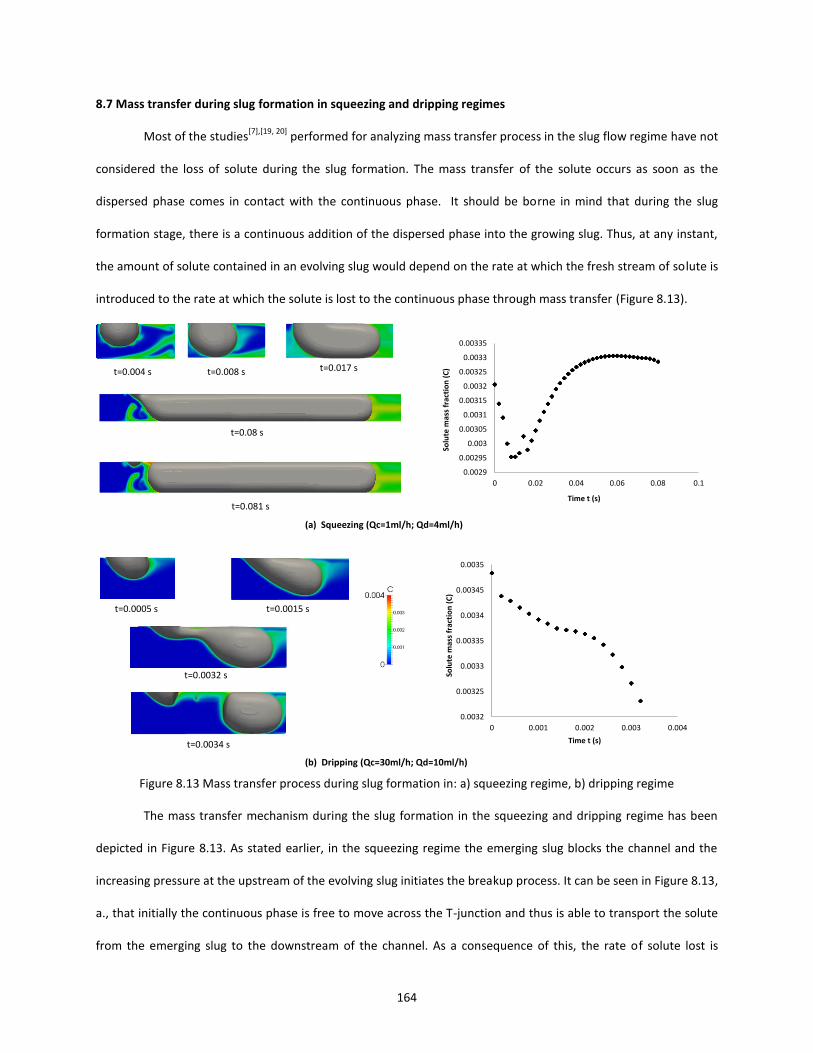
164

8.7 Mass transfer during slug formation in squeezing and dripping regimes

Most of the studies[7],[19, 20]

performed for analyzing mass transfer process in the slug flow regime have not

considered the loss of solute during the slug formation. The mass transfer of the solute occurs as soon as the

dispersed phase comes in contact with the continuous phase. It should be borne in mind that during the slug

formation stage, there is a continuous addition of the dispersed phase into the growing slug. Thus, at any instant,

the amount of solute contained in an evolving slug would depend on the rate at which the fresh stream of solute is

introduced to the rate at which the solute is lost to the continuous phase through mass transfer (Figure 8.13).

Figure 8.13 Mass transfer process during slug formation in: a) squeezing regime, b) dripping regime

The mass transfer mechanism during the slug formation in the squeezing and dripping regime has been

depicted in Figure 8.13. As stated earlier, in the squeezing regime the emerging slug blocks the channel and the

increasing pressure at the upstream of the evolving slug initiates the breakup process. It can be seen in Figure 8.13,

a., that initially the continuous phase is free to move across the T-junction and thus is able to transport the solute

from the emerging slug to the downstream of the channel. As a consequence of this, the rate of solute lost is

0.0029

0.00295

0.003

0.00305

0.0031

0.00315

0.0032

0.00325

0.0033

0.00335

0 0.02 0.04 0.06 0.08 0.1

Solu

te m

ass

frac

tio

n (

C)

Time t (s)

t=0.008 st=0.004 s t=0.017 s

t=0.08 s

t=0.081 s

(a) Squeezing (Qc=1ml/h; Qd=4ml/h)

0.0032

0.00325

0.0033

0.00335

0.0034

0.00345

0.0035

0 0.001 0.002 0.003 0.004

Solu

te m

ass

frac

tio

n (

C)

Time t (s)

t=0.0005 s

t=0.0034 s

t=0.0032 s

t=0.0015 s

(b) Dripping (Qc=30ml/h; Qd=10ml/h)

165

higher than the rate at which solute enters the slug and hence in the initial stages of slug growth the concentration

of solute decreases. The slug gradually blocks the channel and the convective currents wane out and hence the

solute is not quickly displaced from the vicinity of the growing slug and with time the solute concentration

increases which results in reduction in solute concentration gradient between the dispersed and continuous

phases. Thus, mass transfer rate across the interface drops. At the same time the fresh batch of dispersed phase

(containing solute at initial concentration) keeps getting added at a higher rate to the growing slug. Hence, the

concentration of solute in the slug starts increasing. As the slug blocks the channel and further elongates, the mass

transfer primarily occurs through the front cap and the region exposed to the continuous phase upstream to the

evolving slug (thin film region gets saturated and hence mass transfer rate is very low). Thus, right from the instant

slug blocks the channel and causes the increase in solute concentration inside the slug.

In case of dripping regime, the slug disintegration takes place by the action of shear exerted by the

incoming continuous phase on the dispersed phase. The convective current transports the solute to downstream

of the slug and there is continual exposure of the evolving slug to fresh fluid devoid of solute and hence the mass

transfer rates are higher in this case. As it can be seen in Figure 8.13, b., the rate at which the slug loses the solute

is much greater than that entering it and hence for this reason the solute concentration inside the slug registers a

constant fall. When the slug blocks the momentarily, the continuous fluid gets trapped and hence the strength

convection currents drops. This reduces the rate of mass transfer and hence the concentration of solute inside slug

falls at a smaller rate before the shear stress exerted by the continuous fluid forces the interface to elongate and

the slug ultimately disintegrates. Unlike in squeezing regime, the proportion of interfacial area in direct contact

with the bulk of continuous phase is much larger even when the slug momentarily blocks a significant portion of

channel. Further, the convection in this case is much stronger and hence these factors ensure that the slug loses

the solute at a rate greater than with what it gets injected to slug from dispersed phase inlet channel.

8.8 Effect of varying Q on the Mass transfer in channel in squeezing and dripping regimes

In this section, the effect of the varying Q on the mass transfer process during slug formation and its

motion in squeezing and dripping regimes will be described. Figure 8.14 shows the plots for solute concentration

inside the slug and the overall mass transfer coefficients as slug travels in the microchannel during the squeezing

and the dripping regimes. Unlike in squeezing regime, during the dripping regime the slugs are disconnected near

166

the junction of the T-microchannel by the action of shear stresses of the continuous phase. As a consequence, the

slug lengths are comparatively smaller than ones observed in the squeezing regime. It has been previously stated

that the continuous phase trapped in the thin film gets saturated quickly with solute and hence, the majority of

mass transfer occurs through the slug caps. Table 8.4 lists various factors which decide the overall mass transfer of

solute from slug as it traverses in the channel. It can be seen the acap/a, the ratio between the specific area offered

by the cap to total specific area is much higher of slugs in dripping regime.

Figure 8.14 Temporal plots for solute concentration in a travelling slug and overall mass transfer coefficient for a)

dripping regime and b) squeezing regime.

The higher acap/a ratios and slug velocities (see Table 8.3) allow the slugs to lose the solute at a quicker

rate during the dripping regime. This is evident from solute concentration plot in Figure 8.14. It can be observed

for both the regimes that the concentration plots becomes flatter as slugs approach the end of channel suggesting

that the mass transfer rate drops. This is attributed to the fall in the concentration gradient between the dispersed

and continuous phases due to the a) continuous loss of solute in the slug and b) due to build-up of solute

concentration in the continuous phase (refer Figure 8.4). This is reflected in the values of overall mass transfer

0

0.001

0.002

0.003

0.004

0.005

0.006

0.007

0.008

0.009

0.01

0 0.1 0.2 0.3 0.4

k d(m

/s)

Time t (s)

Slug formation

Slug motion

0.00225

0.00235

0.00245

0.00255

0.00265

0.00275

0.00285

0.00295

0 0.1 0.2 0.3 0.4

Solu

te f

ract

ion

C

Time t (s)

Slug formation

Slug motion

(b) Squeezing (Qc=1ml/h; Qd=2ml/h)

0.0015

0.002

0.0025

0.003

0.0035

0 0.005 0.01 0.015 0.02 0.025

Solu

te f

ract

ion

C

Time t (s)

Slug formation

Slug motion

(a) Dripping(Qc=30ml/h; Qd= 10ml/h)

0

0.001

0.002

0.003

0.004

0.005

0.006

0.007

0.008

0.009

0 0.005 0.01 0.015 0.02 0.025

k d(m

/s)

Time t (s)

Slug formation

Slug motion

167

coefficient kd (Figure 8.14), which is highest during the slug formation stage when the concentration gradients

between the phases are maximum. Thereafter, the values of kd drop gradually. It can be inferred from Figure 8.14

that during dripping regime, the amount of solute lost during the slug motion is much higher than that during slug

formation. However, solute lost during the slug formation stage is significant for the flow scenarios with very low

where Qd (refer the values of %lost_formation for flow scenarios with Qd=2ml/h in Table 8.4) .

Table 8.4 Parameters affecting mass transfer from slug during dripping and squeezing regime

Regime Qc (ml/h) Qd (ml/h) Q kda (s-1

) %lost_formation a(m2/m

3) acap/a (%)

S 1 2 2 0.71 29.66 6958 11.22

S 1 4 4 2.50 17.84 7572 16.57

S 1 6 6 3.30 13.32 7865 11.98

S 2 6 3 3.66 15.50 7334 20.48

S 4 6 1.5 3.95 16.84 6849 29.11

D 22 10 0.455 7.29 17.72 5163 50.41

D 26 10 0.385 7.94 18.13 4850 45.61

D 30 2 0.067 3.21 46.32 1379 59.86

D 30 6 0.200 5.84 24.88 3186 55.79

D 30 10 0.333 8.30 19.19 4623 59.82

The effect of varying flow rate ratio Q at a constant Ca (depends on Qc) on the mass transfer from the slug

in dripping regime has been shown in Figure 8.15. In each case the dimensionless time is defined as ⁄ . The

time required for formation of slug is lot higher (approximately 3 times) for Qd= 2ml/h (Q=0.067) when compared

to case where Qd = 10ml/h (Q=0.333). Hence, the growing slug is exposed to the continuous phase being injected

at Qc = 30ml/h (Re=39) for longer duration and hence loses more solute. This explains the lower values of C

observed for Qd = 2ml/h case. A glimpse at the kd plot during slug formation reveals that the kd constantly

decreases for the Q=0.333. However, for Q=0.067 it rises to a peak before registering a steep fall. This can be

explained from Figure 8.16 which shows the contour plots for and C during the slug formation stage. In case of

Q=0.333, the growing slug is able to block the channel cross-section quickly ( =1.08) and the resistance to flow

experienced by the continuous phase causes kd to fall. However, when Qd is introduced at lower flow rate, the slug

grows at a smaller pace and the continuous phase devoid of the solute is able to strip it from the dispersed phase

for a longer duration. As the slug gradually grows the velocity of continuous phase increases in the vicinity of the

emerging slug, due to reduction of area available for flow. This helps to increase kd for a brief period. Gradually

168

with time, the dispersed phase blocks the channel the increased resistance to continuous phase flow leads to

lowering of kd.

In case of the detached slug in motion, kd is higher for Qd= 2ml/h because of the higher (see Table

8.3), which is a measure of distance of separation between the two consecutive slugs. The higher helps in

keeping the solute concentration in continuous phase at a lower value (more dilution) and hence comparatively

larger concentration gradient available to slug yields higher values of kd.

Figure 8.15 Effect of varying Qd on solute concentration and mass transfer coefficient in the slug during its formation and motion in dripping regime (Qc= 30ml/h; Ca= 0.0056).

0

0.001

0.002

0.003

0.004

0.005

0.006

0.007

0.008

0.009

0 2 4 6 8 10

kd

(1

/s)

Dimensionless time t

Qd = 2ml/h

Qd= 10ml/h

0.002

0.0022

0.0024

0.0026

0.0028

0.003

0.0032

0.0034

0.0036

0.0038

0 2 4 6 8

So

lute

ma

ss f

racti

on

C

Dimensionless time t

Qd = 2ml/h

Qd= 10ml/h

0

0.0005

0.001

0.0015

0.002

0.0025

0.003

0.0035

0 5 10 15 20 25

So

lute

Ma

ss f

racti

on

C

Dimensionless time t

Qd = 2ml/h

Qd= 10ml/h

(a) Slug formation

(b) Slug motion

0.0015

0.002

0.0025

0.003

0.0035

0.004

0 5 10 15 20 25

kd

(1

/s)

Dimensionless time t

Qd = 2ml/h

Qd= 10ml/h

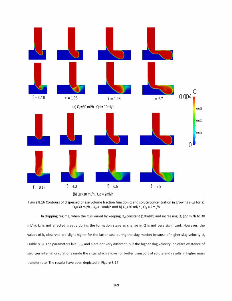
169

Figure .1 Contours of dispersed phase volume fraction function α and solute concentration in growing slug for a)

Qc=30 ml/h , Qd = 10ml/h and b) Qc=30 ml/h , Qd = 2ml/h

In dripping regime, when the Q is varied by keeping Qd constant (10ml/h) and increasing Qc (22 ml/h to 30

ml/h), kd is not affected greatly during the formation stage as change in Q is not very significant. However, the

values of kd observed are slight higher for the latter case during the slug motion because of higher slug velocity Us

(Table 8.3). The parameters like and are not very different, but the higher slug velocity indicates existence of

stronger internal circulations inside the slugs which allows for better transport of solute and results in higher mass

transfer rate. The results have been depicted in Figure 8.17.

(a) Qc=30 ml/h , Qd = 10ml/h

.8

(b) Qc=30 ml/h , Qd = 2ml/h

170

Figure 8.17 Effect of varying Qc on mean solute concentration and mass transfer coefficient in the slug during its formation and motion in dripping regime (Qd= 10ml/h).

The effect of Q variation in squeezing regime on the slug concentration and mass transfer coefficient has

been shown in Figure 8.18 and Figure 8.19. Since the flow rates at which the continuous phase is injected is fairly

low the effect of Q on kd is not very strong. However, the influence of varying Q on kd is more pronounced when

the slug is moving in the microchannel. When Q is varied by changing Qd (with Qc constant), the slug length

increases with increasing Qd. For the flow rates of Qc= 1ml/h and Qd =6ml/h, the flow enters elongated slug regime

where the slug lengths are significantly large. A higher kd observed (Figure 8.18) for case where dispersed phase is

injected at a higher flow rate is attributed to a higher slug velocity which ultimately enhances mass transfer rate.

When Qd is kept constant and Qc is varied, the slug length decreases with increasing Qc. The higher shear stress

exerted by the continuous phase when Qc is increased, helps in increasing kd during the slug motion stage.

0.0031

0.0032

0.0033

0.0034

0.0035

0.0036

0 1 2 3 4

Solu

te m

ass

frac

tio

n C

Dimensionless time t

Qc = 22ml/h

Qc = 30ml/h

0.0015

0.0017

0.0019

0.0021

0.0023

0.0025

0.0027

0.0029

0.0031

0.0033

0.0035

0 5 10 15 20

Solu

te m

ass

frac

tio

n C

Dimensionless time t

Qc = 22ml/h

Qc= 30ml/h

0.003

0.0035

0.004

0.0045

0.005

0.0055

0.006

0.0065

0.007

0.0075

0.008

0 0.5 1 1.5 2 2.5 3

k d (

1/s

)

Dimensionless time t

Qc = 22ml/h

Qc= 30ml/h

(a) Slug formation

(b) Slug motion

0.001

0.0015

0.002

0.0025

0.003

0.0035

0.004

0 5 10 15 20

k d (

1/s

)

Dimensionless time t

Qc = 22ml/h

Qc= 30ml/h

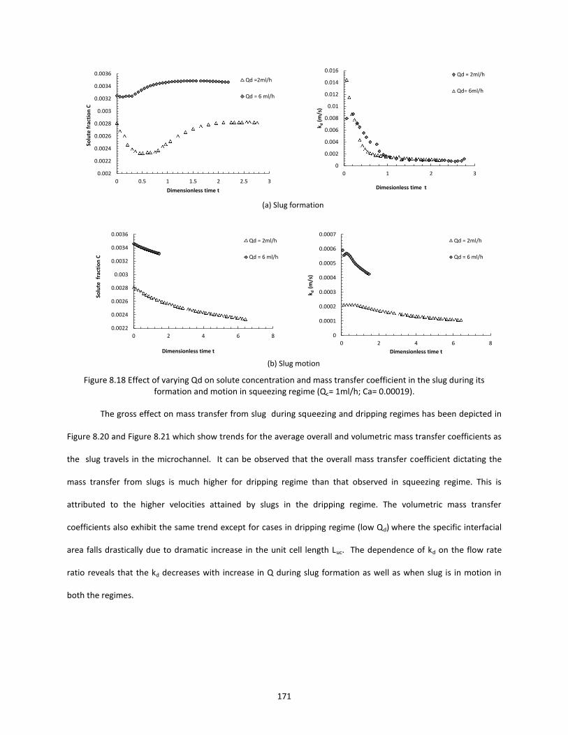
171

Figure 8.18 Effect of varying Qd on solute concentration and mass transfer coefficient in the slug during its

formation and motion in squeezing regime (Qc= 1ml/h; Ca= 0.00019).

The gross effect on mass transfer from slug during squeezing and dripping regimes has been depicted in

Figure 8.20 and Figure 8.21 which show trends for the average overall and volumetric mass transfer coefficients as

the slug travels in the microchannel. It can be observed that the overall mass transfer coefficient dictating the

mass transfer from slugs is much higher for dripping regime than that observed in squeezing regime. This is

attributed to the higher velocities attained by slugs in the dripping regime. The volumetric mass transfer

coefficients also exhibit the same trend except for cases in dripping regime (low Qd) where the specific interfacial

area falls drastically due to dramatic increase in the unit cell length Luc. The dependence of kd on the flow rate

ratio reveals that the kd decreases with increase in Q during slug formation as well as when slug is in motion in

both the regimes.

Squeezing regime Qc=1ml/h

0.002

0.0022

0.0024

0.0026

0.0028

0.003

0.0032

0.0034

0.0036

0 0.5 1 1.5 2 2.5 3

Solu

te f

ract

ion

C

Dimensionless time t

Qd =2ml/h

Qd = 6 ml/h

0

0.002

0.004

0.006

0.008

0.01

0.012

0.014

0.016

0 1 2 3

k d(m

/s)

Dimesionless time t

Qd = 2ml/h

Qd= 6ml/h

0.0022

0.0024

0.0026

0.0028

0.003

0.0032

0.0034

0.0036

0 2 4 6 8

Solu

te f

ract

ion

C

Dimensionless time t

Qd = 2ml/h

Qd = 6 ml/h

(a) Slug formation

(b) Slug motion

0

0.0001

0.0002

0.0003

0.0004

0.0005

0.0006

0.0007

0 2 4 6 8

k d (

m/s

)

Dimensionless time t

Qd = 2ml/h

Qd = 6 ml/h

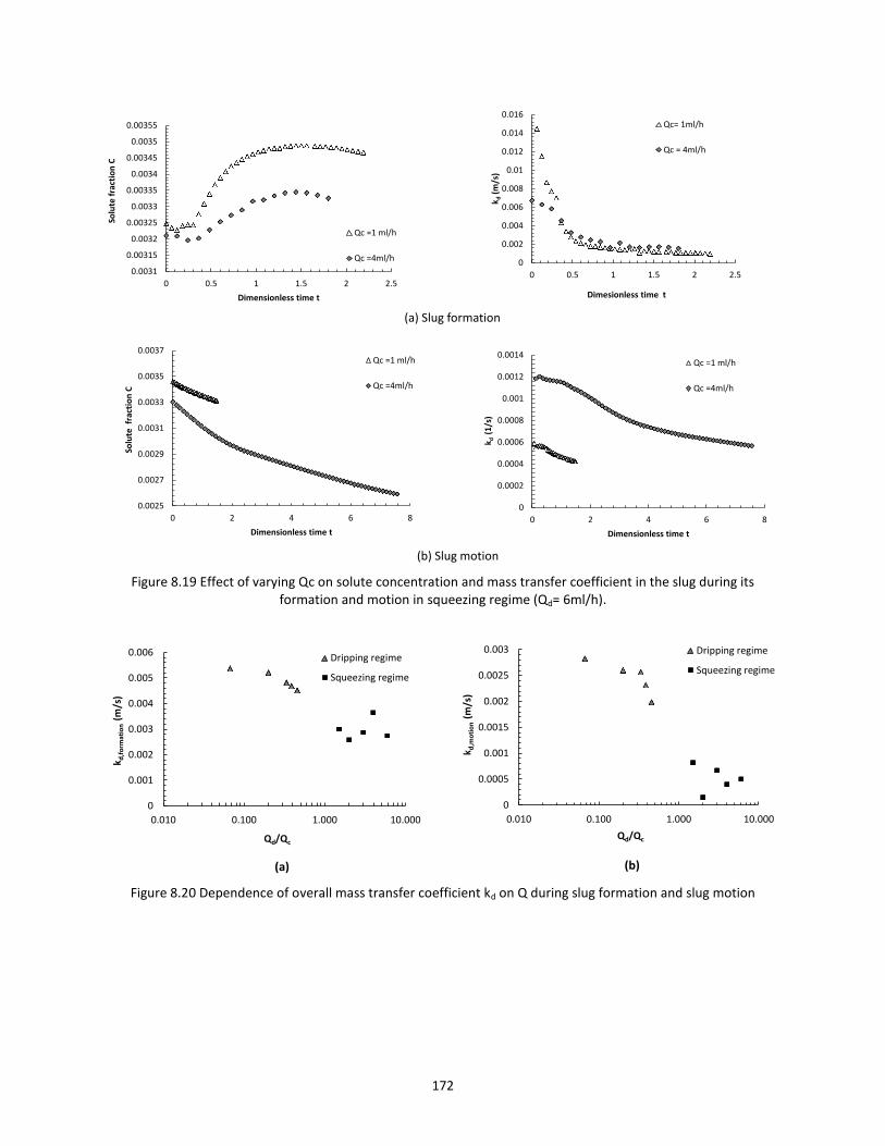
172

Figure 8.19 Effect of varying Qc on solute concentration and mass transfer coefficient in the slug during its

formation and motion in squeezing regime (Qd= 6ml/h).

Figure 8.20 Dependence of overall mass transfer coefficient kd on Q during slug formation and slug motion

0.0031

0.00315

0.0032

0.00325

0.0033

0.00335

0.0034

0.00345

0.0035

0.00355

0 0.5 1 1.5 2 2.5

Solu

te f

ract

ion

C

Dimensionless time t

Qc =1 ml/h

Qc =4ml/h

0.0025

0.0027

0.0029

0.0031

0.0033

0.0035

0.0037

0 2 4 6 8

Solu

te f

ract

ion

C

Dimensionless time t

Qc =1 ml/h

Qc =4ml/h

0

0.002

0.004

0.006

0.008

0.01

0.012

0.014

0.016

0 0.5 1 1.5 2 2.5

k d(m

/s)

Dimesionless time t

Qc= 1ml/h

Qc = 4ml/h

(b) Slug motion

(a) Slug formation

0

0.0002

0.0004

0.0006

0.0008

0.001

0.0012

0.0014

0 2 4 6 8

k d (

1/s

)

Dimensionless time t

Qc =1 ml/h

Qc =4ml/h

0

0.001

0.002

0.003

0.004

0.005

0.006

0.010 0.100 1.000 10.000

k d,f

orm

atio

n (

m/s

)

Qd/Qc

Dripping regime

Squeezing regime

(a) (b)

0

0.0005

0.001

0.0015

0.002

0.0025

0.003

0.010 0.100 1.000 10.000

k d,m

oti

on

(m

/s)

Qd/Qc

Dripping regime

Squeezing regime

173

Figure 8.21 Dependence of overall mass transfer coefficient kd and volumetric mass transfer coefficient kda on slug

velocity in squeezing and dripping regimes

8.9 Conclusions

In this chapter, we have described the mass transfer process of solute from the slugs travelling a T-

microchannel, to the continuous phase. A numerical model developed by integrating traditional VOF approach

with modified species transport equation has been employed for studying the mass transport process. In this

study, mass transfer from slugs in squeezing regime and dripping regimes has been considered. The slugs are

generated by the interaction of the continuous and the dispersed phase at the junction in the microchannel. In

dripping regime, the slugs are produced by the shear stresses exerted by the continuous phase on the emerging

dispersed phase. In contrast, during squeezing regime the dispersed phase completely blocks the channel and

continuous phase experiences resistance to flow. This causes the pressure to rise in the upstream of the evolving

dispersed phase which initiates the slug breakup process. With the physical properties kept constant; the length of

slugs produced primarily depends on the flow rate ratio Q. It is observed that slug length increases with increase

in Q; increase being more prominent with slugs in squeezing regime. Specific area also exhibits similar dependence

on the flow ratio with increase being more significant in dripping regime.

The concentration fields were evaluated from the developed numerical model accounting for the mass

transfer from slugs to continuous phase. The results from numerical simulations indicated that the mean

concentration of the solute during the slug formation in the squeezing regime initially increased because the rate

at which solute is added to the growing slug from the dispersed phase inlet is larger than the rate which solute is

(a) (b)

0

1

2

3

4

5

6

7

8

9

0.01 0.1 1

k d,a

(1/s

)

Us (m/s)

Dripping regime

Squeezing regime

0

0.0005

0.001

0.0015

0.002

0.0025

0.003

0.01 0.1 1

k d,m

oti

on

(m

/s)

Us (m/s)

Dripping regime

Squeezing regime

174

lost to the continuous phase. However, during the slug motion the solute concentration gradually decreased with

the mass transfer rate falling as slug approached the end of channel due to reduced concentration gradients. In the

dripping regime, the shear due to the continuous phase entering the channel at a higher flow rate caused the

mean solute concentration to decrease during both slug formation and slug motion. The simulation results also

revealed that mass of solute lost during the slug formation is significant for squeezing regime and for low dispersed

phase flow rates in the dripping regime.

The effect of varying Q on the overall mass transfer coefficients was also analyzed. It was observed that

the average kd decreased with increase in flow rate ratio during slug formation as well as during slug motion stages

in both squeezing and dripping regimes. It was found that for the moving slug, the value of kd has a direct

dependence on the its velocity Us. Higher the value of Us, higher is the value of kd, the change being more evident

in the dripping regime.

8.10 Nomenclature

a : Specific interfacial area, [m2/m

3].

: Hydraulic diameter of the micro-channel, [m].

: Concentration of solute in continuous phase, [kmol/m3].

: Concentration of solute in dispersed phase, [kmol/m3].

: Concentration of mixture, [-].

: Diffusivity of solute in continuous phase, [m2/s].

: Diffusivity of solute in dispersed phase, [m2/s].

: Diffusivity of mixture, [m2/s].

: Overall mass transfer coefficient [m/s].

: Overall volumetric mass transfer coefficient [1/s].

: Length of film, [m].

: Slug length, [m].

: Length of the unit cell, [m].

175

: Mass transfer rate [kg/m2.s].

m : Partition coefficient.

Q : Volumetric flow rate, [m3/s].

: Area normal vector, [m2].

: Time required for the formation of slug, [m/s].

: Slug velocity, [m/s].

: Interpolated velocity on the face of the control volume, [m/s].

: Velocity field, [m/s].

: Compression velocity, [m/s].

Greek alphabets

: Volume of fraction of dispersed phase

: Film thickness, [m].

: Surface curvature

: Density of continuous phase, [kg/m3].

: Density of dispersed phase, [kg/m3].

: Density of solute, [kg/m3].

: Viscosity of continuous phase [kg/m.s].

: Viscosity of dispersed phase [kg/m.s].

Non dimensional Number

: Reynolds Number

Ca : Capillary Number

Fo : Fourier Number

8.11 References

[1] Y. Su, G. Chen, Q. Yuan, Effect of Viscosity on the Hydrodynamics of Liquid Processes in Microchannels, Chemical Engineering & Technology, 37 (2014) 427-434.

[2] D.M. Fries, T. Voitl, P.R. von Rohr, Liquid Extraction of Vanillin in Rectangular Microreactors, Chemical Engineering & Technology, 31 (2008) 1182-1187.

176

[3] M.T. Kreutzer, A. Günther, K.F. Jensen, Sample Dispersion for Segmented Flow in Microchannels with Rectangular Cross Section, Analytical Chemistry, 80 (2008) 1558-1567.

[4] M. N. Kashid, A. Renken, L. Kiwi-Minsker, Influence of Flow Regime on Mass Transfer in Different Types of Microchannels, Industrial & Engineering Chemistry Research, 50 (2011) 6906-6914.

[5] J. Yun, Q. Lei, S. Zhang, S. Shen, K. Yao, Slug flow characteristics of gas–miscible liquids in a rectangular microchannel with cross and T-shaped junctions, Chemical Engineering Science, 65 (2010) 5256-5263.

[6] F.Y. Ushikubo, F.S. Birribilli, D.R.B. Oliveira, R.L. Cunha, Y- and T-junction microfluidic devices: effect of fluids and interface properties and operating conditions, Microfluid Nanofluid, 17 (2014) 711-720.

[7] D. Tsaoulidis, P. Angeli, Effect of channel size on mass transfer during liquid–liquid plug flow in small scale extractors, Chemical Engineering Journal, 262 (2015) 785-793.

[8] M.N. Kashid, D.W. Agar, Hydrodynamics of liquid–liquid slug flow capillary microreactor: Flow regimes, slug size and pressure drop, Chemical Engineering Journal, 131 (2007) 1-13.

[9] A. Ghaini, A. Mescher, D.W. Agar, Hydrodynamic studies of liquid–liquid slug flows in circular microchannels, Chemical Engineering Science, 66 (2011) 1168-1178.

[10] P. Garstecki, M.J. Fuerstman, H.A. Stone, G.M. Whitesides, Formation of droplets and bubbles in a microfluidic T-junction-scaling and mechanism of break-up, Lab on a Chip, 6 (2006) 437-446.

[11] Y. Zhao, G. Chen, Q. Yuan, Liquid-liquid two-phase flow patterns in a rectangular microchannel, AIChE Journal, 52 (2006) 4052-4060.

[12] M. De Menech, P. Garstecki, F. Jousse, H.A. Stone, Transition from squeezing to dripping in a microfluidic T-shaped junction, Journal of Fluid Mechanics, 595 (2008) 141-161.

[13] P. Aussillous, D. Quéré, Quick deposition of a fluid on the wall of a tube, Physics of Fluids, 12 (2000) 2367-2371.

[14] J.M. van Baten, R. Krishna, CFD simulations of mass transfer from Taylor bubbles rising in circular capillaries, Chemical Engineering Science, 59 (2004) 2535-2545.

[15] J.U. Brackbill, D.B. Kothe, C. Zemach, A continuum method for modeling surface tension, Journal of Computational Physics, 100 (1992) 335-354.

[16] N. Di Miceli Raimondi, L. Prat, C. Gourdon, J. Tasselli, Experiments of mass transfer with liquid–liquid slug flow in square microchannels, Chemical Engineering Science, 105 (2014) 169-178.

[17] Y. Li, R.K. Reddy, C.S.S.R. Kumar, K. Nandakumar, Computational investigations of the mixing performance inside liquid slugs generated by a microfluidic T-junction, Biomicrofluidics, 8 (2014) 054125.

[18] F. Sarrazin, T. Bonometti, L. Prat, C. Gourdon, J. Magnaudet, Hydrodynamic structures of droplets engineered in rectangular micro-channels, Microfluid Nanofluid, 5 (2008) 131-137.

[19] C. Yao, Z. Dong, Y. Zhao, G. Chen, An online method to measure mass transfer of slug flow in a microchannel, Chemical Engineering Science, 112 (2014) 15-24.

[20] B. Xu, W. Cai, X. Liu, X. Zhang, Mass transfer behavior of liquid–liquid slug flow in circular cross-section microchannel, Chemical Engineering Research and Design, 91 (2013) 1203-1211.

177

Chapter 9 Conclusions and Outlook

9.1 Summary and key contributions

Through this work we have demonstrated that the capabilities of Multiphase CFD modelling can be

harnessed for simulating flows relevant to variety of physical systems. In the first part of this dissertation, we

showed the application of CFD in simulating transport processes associated with deep water oil spills. In the initial

stages different multiphase CFD models were employed for capturing large scale phenomena like fractionation of

multiphase plume in presence of ambient currents, formation of intrusion layers and evaposinking. These

qualitative results have been discussed in Chapter 2. In pursuit of developing an integrated model, the first

objective was to seek a better understanding of these transport processes at a very fundamental level. To

investigate this, in the first phase of this project we studied the effect of surfactant present in the continuous

phase on the dynamics of a single crude oil droplet rising in a stagnant water column through experiments and the

developed numerical model. The results (Chapter 3) revealed that the lowering of interfacial tension at the oil

water interface caused by the increase in the concentration of surfactant, resulted in decrease in aspect ratio of

the droplet, i.e. droplets assumed a more flatter shape and as a consequence, decrease in the rise velocities of the

droplet was observed.

In the subsequent study (Chapter 4), an attempt was made to understand the process of dissolution of

hydrocarbons from the droplet phase in the subsurface. The actual oil droplet was substituted with a binary

organic mixture comprising of a component soluble in water and a component insoluble in water. The initial

mixture density of the droplet (less than that of surrounding medium) allowed the droplet to rise in the column.

However, with the continuous loss of soluble component, the droplet became denser. As a consequence, the

droplet momentarily became stationary when its density was equal to that of water. Further loss of solute caused

the droplet become heavier and it eventually sank. A correlation capable of predicting mass transfer rate at

different stages of droplet motion proposed. A multiphase CFD model was also developed in ANSYS Fluent® for

mimicking the experimental observations. Chapter 5 showcased the extension of the CFD models developed in

chapters 3 and 4 to simulate the effect of surfactant and unsteady mass transfer on the dynamics of the jet in

laminar regime.

178

During the accidental oil releases under the sea the local turbulence and the dispersant addition results in

generation of droplets with wide size distribution. Information on the size distribution is important in estimating

the fate of oil droplets in the water column. To address this, a model (described in Chapter 6) was developed by

bringing in integration of Multiphase CFD model with traditional Population Balance Modelling (PBM) approach.

The model thus developed had the capability to predict the size droplets on the basis of local turbulence and the

interfacial tension at the interface. The model was employed to analyze the effect of dispersed (oil) phase flow

rates, presence of dispersants and presence of gas in the jet phase on the overall size distribution of oil droplets

emerging from a turbulent jet. It was concluded that high oil injection rates and higher concentration of

dispersants assists disintegration process and results in generation of smaller droplets. The presence of air in the

dispersed phase revealed some interesting facts. It was found that at a constant dispersed phase flow rate, lower

energy available to dispersed phase due to the presence of air, resulted in generation of droplets which were

larger than in case where pure phase was injected through the nozzle. However, when the dispersed phase was

introduced with constant momentum flux, it was observed that the presence of air provided additional energy to

the system thereby increasing the dissipation rates and hence yielded smaller droplets than in latter scenario.

In Chapter 7, we described the mass transfer model cstFoam, developed in the open source CFD package

OpenFOAM®, which carried flavours of traditional Volume of Fluid (VOF) and Continuum Surface Force (CSF)

approaches for capturing mass transfer of solute across the interface of two immiscible fluids. This was achieved

by infusing a modified species transport equation into standard interFoam solver. The model was an improvement

over the previously developed model (Chapter 3) in the sense that the mass transfer across the interface was

limited by a specified partition coefficient and did not require a priori information on mass transfer rates. The

implementation of cstFoam to capture the mass transfer from slugs travelling in a microchannel was shown in

Chapter 8. The simulations were performed to study mass transfer process during slug formation and slug motion

stages in the dripping and squeezing regimes. It was observed that the slugs in dripping regime exhibited higher

mass transfer coefficients than that in squeezing regime.

9.2 Future work

In the course of this work we have developed CFD models to capture the major transport processes that

influence the behavior of droplets during the accidental releases in deep sea. A full predictive model for estimating

179

the fate of oil droplets in such events can derive important inputs from these CFD models. The path forward

would be to integrate the developed multiphase CFD models with the models capable of reproducing the flow

fields existing in an actual marine environment. This comprehensive model can be used for predicting droplet

trajectories in the event of accidental events. However, an extensive and reliable field scale experimental data

should be made available for validating such models. In Chapter 6, we demonstrated the use of an integrated CFD

and PB models for simulating meso-scale experiments. The capability of this model can be widened by infusing a

more holistic view to integrated CFD+PB model by introducing equations to account for mass transport in the

existing framework. In Chapter 3, an experimental case, describing the influence of surfactant on the mass transfer

rates of the solute moving from the dispersed to continuous, was presented. The cstFoam model (Chapter7) can

be extended to capture this effect. The cstFoam model currently has provisions for specifying a constant surface

tension. In actual cases the amount of adsorption of surfactant may vary along the oil-water interface of the

droplet/jet. This difference in adsorption sets up the gradient in the surface tension which results in bulk motion of

fluid from region of low interfacial tension to region of high interfacial tension along the interface (Marangoni

convection). At fundamental scale of droplets/jets in laminar regime, Marangoni convection can be important in

some scenarios. The current cstFoam solver can be modified for imposing surface tension in accordance to the

local surfactant concentration. To capture the Marangoni convection provision has to be made to include

additional tangential stress terms in the momentum equation.

180

Appendix A File organization in cstFoam solver

Various files that comprise cstFoam solver have been listed below.

A.1 alphaCourantNo.H

/*---------------------------------------------------------------------------

*\

========= |

\\ / F ield | OpenFOAM: The Open Source CFD Toolbox

\\ / O peration |

\\ / A nd | Copyright (C) 2011-2014 OpenFOAM Foundation

\\/ M anipulation |

-----------------------------------------------------------------------------

--

License

This file is part of OpenFOAM.

OpenFOAM is free software: you can redistribute it and/or modify it

under the terms of the GNU General Public License as published by

the Free Software Foundation, either version 3 of the License, or

(at your option) any later version.

OpenFOAM is distributed in the hope that it will be useful, but WITHOUT

ANY WARRANTY; without even the implied warranty of MERCHANTABILITY or

FITNESS FOR A PARTICULAR PURPOSE. See the GNU General Public License

for more details.

You should have received a copy of the GNU General Public License

along with OpenFOAM. If not, see <http://www.gnu.org/licenses/>.

Global

alphaCourantNo

Description

Calculates and outputs the mean and maximum Courant Numbers.

\*---------------------------------------------------------------------------

*/

scalar maxAlphaCo

(

readScalar(runTime.controlDict().lookup("maxAlphaCo"))

);

scalar alphaCoNum = 0.0;

scalar meanAlphaCoNum = 0.0;

if (mesh.nInternalFaces())

{

scalarField sumPhi

(

mixture.nearInterface()().internalField()

*fvc::surfaceSum(mag(phi))().internalField()

);

181

alphaCoNum = 0.5*gMax(sumPhi/mesh.V().field())*runTime.deltaTValue();

meanAlphaCoNum =

0.5*(gSum(sumPhi)/gSum(mesh.V().field()))*runTime.deltaTValue();

}

Info<< "Interface Courant Number mean: " << meanAlphaCoNum

<< " max: " << alphaCoNum << endl;

// *************************************************************************

//

A.2 alphaEqn.H

{

word alphaScheme("div(phi,alpha)");

word alpharScheme("div(phirb,alpha)");

// Standard face-flux compression coefficient

surfaceScalarField phic(mixture.cAlpha()*mag(phi/mesh.magSf()));

// Add the optional isotropic compression contribution

if (icAlpha > 0)

{

phic *= (1.0 - icAlpha);

phic += (mixture.cAlpha()*icAlpha)*fvc::interpolate(mag(U));

}

// Do not compress interface at non-coupled boundary faces

// (inlets, outlets etc.)

forAll(phic.boundaryField(), patchi)

{

fvsPatchScalarField& phicp = phic.boundaryField()[patchi];

if (!phicp.coupled())

{

phicp == 0;

}

}

tmp<surfaceScalarField> tphiAlpha;

if (MULESCorr)

{

fvScalarMatrix alpha1Eqn

(

#ifdef LTSSOLVE

fv::localEulerDdtScheme<scalar>(mesh,

rDeltaT.name()).fvmDdt(alpha1)

#else

fv::EulerDdtScheme<scalar>(mesh).fvmDdt(alpha1)

#endif

+ fv::gaussConvectionScheme<scalar>

(

mesh,

phi,

upwind<scalar>(mesh, phi)

182

).fvmDiv(phi, alpha1)

);

alpha1Eqn.solve();

Info<< "Phase-1 volume fraction = "

<< alpha1.weightedAverage(mesh.Vsc()).value()

<< " Min(alpha1) = " << min(alpha1).value()

<< " Max(alpha1) = " << max(alpha1).value()

<< endl;

tmp<surfaceScalarField> tphiAlphaUD(alpha1Eqn.flux());

tphiAlpha = tmp<surfaceScalarField>

(

new surfaceScalarField(tphiAlphaUD())

);

if (alphaApplyPrevCorr && tphiAlphaCorr0.valid())

{

Info<< "Applying the previous iteration compression flux" <<

endl;

#ifdef LTSSOLVE

MULES::LTScorrect(alpha1, tphiAlpha(), tphiAlphaCorr0(), 1, 0);

#else

MULES::correct(alpha1, tphiAlpha(), tphiAlphaCorr0(), 1, 0);

#endif

tphiAlpha() += tphiAlphaCorr0();

}

// Cache the upwind-flux

tphiAlphaCorr0 = tphiAlphaUD;

alpha2 = 1.0 - alpha1;

mixture.correct();

}

for (int aCorr=0; aCorr<nAlphaCorr; aCorr++)

{

surfaceScalarField phir(phic*mixture.nHatf());

tmp<surfaceScalarField> tphiAlphaUn

(

fvc::flux

(

phi,

alpha1,

alphaScheme

)

+ fvc::flux

(

-fvc::flux(-phir, alpha2, alpharScheme),

alpha1,

alpharScheme

)

);

183

if (MULESCorr)

{

tmp<surfaceScalarField> tphiAlphaCorr(tphiAlphaUn() -

tphiAlpha());

volScalarField alpha10(alpha1);

#ifdef LTSSOLVE

MULES::LTScorrect(alpha1, tphiAlphaUn(), tphiAlphaCorr(), 1, 0);

#else

MULES::correct(alpha1, tphiAlphaUn(), tphiAlphaCorr(), 1, 0);

#endif

// Under-relax the correction for all but the 1st corrector

if (aCorr == 0)

{

tphiAlpha() += tphiAlphaCorr();

}

else

{

alpha1 = 0.5*alpha1 + 0.5*alpha10;

tphiAlpha() += 0.5*tphiAlphaCorr();

}

}

else

{

tphiAlpha = tphiAlphaUn;

#ifdef LTSSOLVE

MULES::explicitLTSSolve(alpha1, phi, tphiAlpha(), 1, 0);

#else

MULES::explicitSolve(alpha1, phi, tphiAlpha(), 1, 0);

#endif

}

alpha2 = 1.0 - alpha1;

mixture.correct();

}

rhoPhi = tphiAlpha()*(rho1 - rho2) + phi*rho2;

if (alphaApplyPrevCorr && MULESCorr)

{

tphiAlphaCorr0 = tphiAlpha() - tphiAlphaCorr0;

}

Info<< "Phase-1 volume fraction = "

<< alpha1.weightedAverage(mesh.Vsc()).value()

<< " Min(alpha1) = " << min(alpha1).value()

<< " Max(alpha1) = " << max(alpha1).value()

<< endl;

}

A.3 alphaEqnSubCycle.H

if (nAlphaSubCycles > 1)

184

{

dimensionedScalar totalDeltaT = runTime.deltaT();

surfaceScalarField rhoPhiSum

(

IOobject

(

"rhoPhiSum",

runTime.timeName(),

mesh

),

mesh,

dimensionedScalar("0", rhoPhi.dimensions(), 0)

);

for

(

subCycle<volScalarField> alphaSubCycle(alpha1, nAlphaSubCycles);

!(++alphaSubCycle).end();

)

{

#include "alphaEqn.H"

rhoPhiSum += (runTime.deltaT()/totalDeltaT)*rhoPhi;

}

rhoPhi = rhoPhiSum;

}

else

{

#include "alphaEqn.H"

}

rho == (1-C)*alpha1*rho1 + (1-C)*alpha2*rho2 + C*alpha2*rhoc + C*alpha1*rhoc;

// ADDED ----------------------------->

//rhoCp == alpha1*rho1*cp1 + alpha2*rho2*cp2;

// ADDED -----------------------------<

A.4 CEqn.H

surfaceScalarField Dcf = mixture.Dcf();

volScalarField Dc = mixture.Dc();

surfaceScalarField phiC = fvc::interpolate((Dc1 - Dc2/He)/(alpha1 +(1-

alpha1)/He))*fvc::snGrad(alpha1)*mesh.magSf();

surfaceScalarField phiD = fvc::snGrad(Dc)*mesh.magSf();

fvScalarMatrix CEqn

(

fvm::ddt(C)

+ fvm::div(phi, C)

- fvm::laplacian(Dcf, C)

+ fvm::div(phiC, C)

- fvm::div(phiD, C)

);

CEqn.solve()

185

A.5 correctPhi.H

{

#include "continuityErrs.H"

volScalarField pcorr

(

IOobject

(

"pcorr",

runTime.timeName(),

mesh,

IOobject::NO_READ,

IOobject::NO_WRITE

),

mesh,

dimensionedScalar("pcorr", p_rgh.dimensions(), 0.0),

pcorrTypes

);

dimensionedScalar rAUf("rAUf", dimTime/rho.dimensions(), 1.0);

adjustPhi(phi, U, pcorr);

while (pimple.correctNonOrthogonal())

{

fvScalarMatrix pcorrEqn

(

fvm::laplacian(rAUf, pcorr) == fvc::div(phi)

);

pcorrEqn.setReference(pRefCell, pRefValue);

pcorrEqn.solve();

if (pimple.finalNonOrthogonalIter())

{

phi -= pcorrEqn.flux();

}

}

#include "continuityErrs.H"

}

A.6 createFields.H

// ADDED ------------------------------------------>

Info<< "Reading transportProperties\n" << endl;

IOdictionary transportProperties

(

IOobject

(

"transportProperties",

runTime.constant(),

mesh,

IOobject::MUST_READ_IF_MODIFIED,

IOobject::NO_WRITE

186

)

);

// ADDED <------------------------------------------

dimensionedScalar He

(

transportProperties.lookup("He")

);

dimensionedScalar rhoc

(

transportProperties.lookup("rhoc")

);

Info<< "Reading field p_rgh\n" << endl;

volScalarField p_rgh

(

IOobject

(

"p_rgh",

runTime.timeName(),

mesh,

IOobject::MUST_READ,

IOobject::AUTO_WRITE

),

mesh

);

// ADDED ------------------------------------------>

Info<< "Reading field C\n" << endl;

volScalarField C

(

IOobject

(

"C",

runTime.timeName(),

mesh,

IOobject::MUST_READ,

IOobject::AUTO_WRITE

),

mesh

);

// ADDED <------------------------------------------

Info<< "Reading field U\n" << endl;

volVectorField U

(

IOobject

(

"U",

runTime.timeName(),

mesh,

IOobject::MUST_READ,

IOobject::AUTO_WRITE

),

mesh

187

);

#include "createPhi.H"

Info<< "Reading transportProperties\n" << endl;

immiscibleIncompressibleTwoPhaseMixture mixture(U, phi);

volScalarField& alpha1(mixture.alpha1());

volScalarField& alpha2(mixture.alpha2());

const dimensionedScalar& rho1 = mixture.rho1();

const dimensionedScalar& rho2 = mixture.rho2();

// ADDED ------------------------------------------>

const dimensionedScalar& Dc1 = mixture.Dc1();

const dimensionedScalar& Dc2 = mixture.Dc2();

// ADDED <------------------------------------------

// Need to store rho for ddt(rho, U)

volScalarField rho

(

IOobject

(

"rho",

runTime.timeName(),

mesh,

IOobject::READ_IF_PRESENT,

IOobject::AUTO_WRITE

),

(1-C)*alpha1*rho1 + (1-C)*alpha2*rho2 + C*alpha2*rhoc +

C*alpha1*rhoc,

alpha1.boundaryField().types()

);

rho.oldTime();

// Mass flux

surfaceScalarField rhoPhi

(

IOobject

(

"rhoPhi",

runTime.timeName(),

mesh,

IOobject::NO_READ,

IOobject::NO_WRITE

),

fvc::interpolate(rho)*phi

);

// Construct incompressible turbulence model

autoPtr<incompressible::turbulenceModel> turbulence

(

incompressible::turbulenceModel::New(U, phi, mixture)

);

#include "readGravitationalAcceleration.H"

188

Info<< "Calculating field g.h\n" << endl;

volScalarField gh("gh", g & mesh.C());

surfaceScalarField ghf("ghf", g & mesh.Cf());

volScalarField p

(

IOobject

(

"p",

runTime.timeName(),

mesh,

IOobject::NO_READ,

IOobject::AUTO_WRITE

),

p_rgh + rho*gh

);

label pRefCell = 0;

scalar pRefValue = 0.0;

setRefCell

(

p,

p_rgh,

mesh.solutionDict().subDict("PIMPLE"),

pRefCell,

pRefValue

);

if (p_rgh.needReference())

{

p += dimensionedScalar

(

"p",

p.dimensions(),

pRefValue - getRefCellValue(p, pRefCell)

);

p_rgh = p - rho*gh;

}

fv::IOoptionList fvOptions(mesh);

// MULES Correction

tmp<surfaceScalarField> tphiAlphaCorr0;

A.7 cstFoam.C

/*-------------------------------------------------------------------------

--*\

========= |

\\ / F ield | OpenFOAM: The Open Source CFD Toolbox

\\ / O peration |

189

\\ / A nd | Copyright (C) 2011-2014 OpenFOAM Foundation

\\/ M anipulation |

-----------------------------------------------------------------------------

--

License

This file is part of OpenFOAM.

OpenFOAM is free software: you can redistribute it and/or modify it

under the terms of the GNU General Public License as published by

the Free Software Foundation, either version 3 of the License, or

(at your option) any later version.

OpenFOAM is distributed in the hope that it will be useful, but WITHOUT

ANY WARRANTY; without even the implied warranty of MERCHANTABILITY or

FITNESS FOR A PARTICULAR PURPOSE. See the GNU General Public License

for more details.

You should have received a copy of the GNU General Public License

along with OpenFOAM. If not, see <http://www.gnu.org/licenses/>.

Application

interFoam

Description

Solver for 2 incompressible, isothermal immiscible fluids using a VOF

(volume of fluid) phase-fraction based interface capturing approach.

The momentum and other fluid properties are of the "mixture" and a single

momentum equation is solved.

Turbulence modelling is generic, i.e. laminar, RAS or LES may be

selected.

For a two-fluid approach see twoPhaseEulerFoam.

\*---------------------------------------------------------------------------

*/

#include "fvCFD.H"

#include "CMULES.H"

#include "subCycle.H"

#include "myImmiscibleIncompressibleTwoPhaseMixture.H"

#include "turbulenceModel.H"

#include "pimpleControl.H"

#include "fvIOoptionList.H"

#include "fixedFluxPressureFvPatchScalarField.H"

// * * * * * * * * * * * * * * * * * * * * * * * * * * * * * * * * * * * * *

//

int main(int argc, char *argv[])

{

#include "setRootCase.H"

#include "createTime.H"

#include "createMesh.H"

pimpleControl pimple(mesh);

190

#include "initContinuityErrs.H"

#include "createFields.H"

#include "readTimeControls.H"

#include "createPrghCorrTypes.H"

#include "correctPhi.H"

#include "CourantNo.H"

#include "setInitialDeltaT.H"

// * * * * * * * * * * * * * * * * * * * * * * * * * * * * * * * * * * *

//

Info<< "\nStarting time loop\n" << endl;

while (runTime.run())

{

#include "readTimeControls.H"

#include "CourantNo.H"

#include "alphaCourantNo.H"

#include "setDeltaT.H"

runTime++;

Info<< "Time = " << runTime.timeName() << nl << endl;

// --- Pressure-velocity PIMPLE corrector loop

while (pimple.loop())

{

#include "alphaControls.H"

#include "alphaEqnSubCycle.H"

mixture.correct();

#include "UEqn.H"

// --- Pressure corrector loop

while (pimple.correct())

{

#include "pEqn.H"

}

if (pimple.turbCorr())

{

turbulence->correct();

}

}

//Added by natali

#include "CEqn.H"

runTime.write();

Info<< "ExecutionTime = " << runTime.elapsedCpuTime() << " s"

<< " ClockTime = " << runTime.elapsedClockTime() << " s"

<< nl << endl;

}

191

Info<< "End\n" << endl;

return 0;

}

// *************************************************************************

//

A.8 pEqn.H

{

volScalarField rAU("rAU", 1.0/UEqn.A());

surfaceScalarField rAUf("rAUf", fvc::interpolate(rAU));

volVectorField HbyA("HbyA", U);

HbyA = rAU*UEqn.H();

surfaceScalarField phiHbyA

(

"phiHbyA",

(fvc::interpolate(HbyA) & mesh.Sf())

+ fvc::interpolate(rho*rAU)*fvc::ddtCorr(U, phi)

);

adjustPhi(phiHbyA, U, p_rgh);

fvOptions.makeRelative(phiHbyA);

surfaceScalarField phig

(

(

mixture.surfaceTensionForce()

- ghf*fvc::snGrad(rho)

)*rAUf*mesh.magSf()

);

phiHbyA += phig;

// Update the fixedFluxPressure BCs to ensure flux consistency

setSnGrad<fixedFluxPressureFvPatchScalarField>

(

p_rgh.boundaryField(),

(

phiHbyA.boundaryField()

- fvOptions.relative(mesh.Sf().boundaryField() & U.boundaryField())

)/(mesh.magSf().boundaryField()*rAUf.boundaryField())

);

while (pimple.correctNonOrthogonal())

{

fvScalarMatrix p_rghEqn

(

fvm::laplacian(rAUf, p_rgh) == fvc::div(phiHbyA)

);

p_rghEqn.setReference(pRefCell, getRefCellValue(p_rgh, pRefCell));

p_rghEqn.solve(mesh.solver(p_rgh.select(pimple.finalInnerIter())));

192

if (pimple.finalNonOrthogonalIter())

{

phi = phiHbyA - p_rghEqn.flux();

p_rgh.relax();

U = HbyA + rAU*fvc::reconstruct((phig - p_rghEqn.flux())/rAUf);

U.correctBoundaryConditions();

fvOptions.correct(U);

}

}

#include "continuityErrs.H"

p == p_rgh + rho*gh;

if (p_rgh.needReference())

{

p += dimensionedScalar

(

"p",

p.dimensions(),

pRefValue - getRefCellValue(p, pRefCell)

);

p_rgh = p - rho*gh;

}

}

A.9 setDelta.H

/*---------------------------------------------------------------------------

*\

========= |

\\ / F ield | OpenFOAM: The Open Source CFD Toolbox

\\ / O peration |

\\ / A nd | Copyright (C) 2011 OpenFOAM Foundation

\\/ M anipulation |

-----------------------------------------------------------------------------

--

License

This file is part of OpenFOAM.

OpenFOAM is free software: you can redistribute it and/or modify it

under the terms of the GNU General Public License as published by

the Free Software Foundation, either version 3 of the License, or

(at your option) any later version.

OpenFOAM is distributed in the hope that it will be useful, but WITHOUT

ANY WARRANTY; without even the implied warranty of MERCHANTABILITY or

FITNESS FOR A PARTICULAR PURPOSE. See the GNU General Public License

for more details.

You should have received a copy of the GNU General Public License

along with OpenFOAM. If not, see <http://www.gnu.org/licenses/>.

Global

193

setDeltaT

Description

Reset the timestep to maintain a constant maximum courant Number.

Reduction of time-step is immediate, but increase is damped to avoid

unstable oscillations.

\*---------------------------------------------------------------------------

*/

if (adjustTimeStep)

{

scalar maxDeltaTFact =

min(maxCo/(CoNum + SMALL), maxAlphaCo/(alphaCoNum + SMALL));

scalar deltaTFact = min(min(maxDeltaTFact, 1.0 + 0.1*maxDeltaTFact),

1.2);

runTime.setDeltaT

(

min

(

deltaTFact*runTime.deltaTValue(),

maxDeltaT

)

);

Info<< "deltaT = " << runTime.deltaTValue() << endl;

}

// *************************************************************************

//

A.10 UEqn.H

fvVectorMatrix UEqn

(

fvm::ddt(rho, U)

+ fvm::div(rhoPhi, U)

+ turbulence->divDevRhoReff(rho, U)

==

fvOptions(rho, U)

);

UEqn.relax();

fvOptions.constrain(UEqn);

if (pimple.momentumPredictor())

{

solve

(

UEqn

==

fvc::reconstruct

(

(

194

mixture.surfaceTensionForce()

- ghf*fvc::snGrad(rho)

- fvc::snGrad(p_rgh)

) * mesh.magSf()

)

);

fvOptions.correct(U);

}

195

Appendix B Problem Setup for cstFoam solver

B.1 ‘0’ directory

This subdirectory houses information on the boundary conditions for various fields included in the

transport equations. Sample files have been illustrated below:

B.1.1 0/alpha

/*--------------------------------*- C++ -*----------------------------------

*\

| ========= |

|

| \\ / F ield | OpenFOAM: The Open Source CFD Toolbox

|

| \\ / O peration | Version: 2.3.x

|

| \\ / A nd | Web: www.OpenFOAM.org

|

| \\/ M anipulation |

|

\*---------------------------------------------------------------------------

*/

FoamFile

{

version 2.0;

format ascii;

class volScalarField;

location "0";

object alpha.toluene;

}

// * * * * * * * * * * * * * * * * * * * * * * * * * * * * * * * * * * * * *

//

dimensions [0 0 0 0 0 0 0];

internalField uniform 0;

boundaryField

{

junction_wall

{

type constantAlphaContactAngle;

theta0 180;

limit gradient;

value uniform 0;

}

continuous_inlet_wall

{

type constantAlphaContactAngle;

theta0 180;

limit gradient;

value uniform 0;

}

196

disp_inlet_wall

{

/*type zeroGradient;*/

type constantAlphaContactAngle;

theta0 120;

limit gradient;

value uniform 0;

}

channel_wall

{

type constantAlphaContactAngle;

theta0 180;

limit gradient;

value uniform 0;

/*type dynamicAlphaContactAngle;

value uniform 0;

theta0 140;

uTheta 0.1; //contact line velocity

thetaA 125;

thetaR 85;

limit gradient;*/

}

outlet

{

type zeroGradient;

}

continuous_inlet

{

type inletOutlet;

inletValue uniform 0;

value uniform 0;

}

dispersed_inlet

{

type inletOutlet;

inletValue uniform 1;

value uniform 1;

}

}

// *************************************************************************

B.1.2 0/C

/*--------------------------------*- C++ -*----------------------------------

*\

| ========= |

|

| \\ / F ield | OpenFOAM: The Open Source CFD Toolbox

|

| \\ / O peration | Version: 2.3.x

|

| \\ / A nd | Web: www.OpenFOAM.org

|

197

| \\/ Manipulation |

|

\*---------------------------------------------------------------------------

*/

FoamFile

{

version 2.0;

format ascii;

class volScalarField;

location "0";

object C;

}

// * * * * * * * * * * * * * * * * * * * * * * * * * * * * * * * * * * * * *

//

dimensions [0 0 0 0 0 0 0];

internalField uniform 0;

boundaryField

{

junction_wall

{

type zeroGradient;

}

continuous_inlet_wall

{

type zeroGradient;

}

disp_inlet_wall

{

type zeroGradient;

}

channel_wall

{

type zeroGradient;

}

outlet

{

type inletOutlet;

inletValue uniform 0;

value uniform 0;

}

continuous_inlet

{

type fixedValue;

value uniform 0;

}

dispersed_inlet

{

type fixedValue;

value uniform 0.004;

}

}

// *************************************************************************

198

B.1.3 0/p_rgh

/*--------------------------------*- C++ -*----------------------------------

*\

| ========= |

|

| \\ / F ield | OpenFOAM: The Open Source CFD Toolbox

|

| \\ / O peration | Version: 2.3.0

|

| \\ / A nd | Web: www.OpenFOAM.org

|

| \\/ Manipulation |

|

\*---------------------------------------------------------------------------

*/

FoamFile

{

version 2.0;

format ascii;

class volScalarField;

object p_rgh;

}

// * * * * * * * * * * * * * * * * * * * * * * * * * * * * * * * * * * * * *

dimensions [1 -1 -2 0 0 0 0];

internalField uniform 0;

boundaryField

{

junction_wall

{

type zeroGradient;

}

continuous_inlet_wall

{

type zeroGradient;

}

disp_inlet_wall

{

type zeroGradient;

}

channel_wall

{

type zeroGradient;

}

outlet

{

type fixedValue;

value uniform 0;

}

continuous_inlet

{

199

type fixedFluxPressure;

value uniform 0;

}

dispersed_inlet

{

type fixedFluxPressure;

value uniform 0;

}

}

// *************************************************************************

B.1.4 0/U

/*--------------------------------*- C++ -*----------------------------------

*\

| ========= |

|

| \\ / F ield | OpenFOAM: The Open Source CFD Toolbox

|

| \\ / O peration | Version: 2.3.0

|

| \\ / A nd | Web: www.OpenFOAM.org

|

| \\/ M anipulation |

|

\*---------------------------------------------------------------------------

*/

FoamFile

{

version 2.0;

format ascii;

class volVectorField;

location "0";

object U;

}

// * * * * * * * * * * * * * * * * * * * * * * * * * * * * * * * * * * * * *

dimensions [0 1 -1 0 0 0 0];

internalField uniform (0 0 0);

boundaryField

{

junction_wall

{

type fixedValue;

value uniform (0 0 0);

}

continuous_inlet_wall

{

type fixedValue;

value uniform (0 0 0);

}

disp_inlet_wall

200

{

type fixedValue;

value uniform (0 0 0);

}

channel_wall

{

type fixedValue;

value uniform (0 0 0);

}

outlet

{

type pressureInletOutletVelocity;

value uniform (0 0 0);

inletValue uniform (0 0 0);

}

continuous_inlet

{

type fixedValue;

value uniform (0.0063 0 0);

}

dispersed_inlet

{

type fixedValue;

value uniform (0 0 -0.0252);

}

}

// *************************************************************************

/

B.2 ‘constant’ directory

B.2.1 constant/transportProperties

/*--------------------------------*- C++ -*----------------------------------*\

| ========= |

|

| \\ / F ield | OpenFOAM: The Open Source CFD Toolbox

|

| \\ / O peration | Version: 2.3.0

|

| \\ / A nd | Web: www.OpenFOAM.org

|

| \\/ M anipulation |

|

\*---------------------------------------------------------------------------

*/

FoamFile

{

version 2.0;

format ascii;

201

class dictionary;

location "constant";

object transportProperties;

}

// * * * * * * * * * * * * * * * * * * * * * * * * * * * * * * * * * * * * *

//

phases (toluene water);

toluene // dispersed phase

{

transportModel Newtonian;

nu nu [ 0 2 -1 0 0 0 0 ] 6.944e-07;

rho rho [ 1 -3 0 0 0 0 0 ] 864;

Dc Dc [ 0 2 -1 0 0 0 0 ] 2.8e-9;

CrossPowerLawCoeffs

{

nu0 nu0 [ 0 2 -1 0 0 0 0 ] 1e-06;

nuInf nuInf [ 0 2 -1 0 0 0 0 ] 1e-06;

m m [ 0 0 1 0 0 0 0 ] 1;

n n [ 0 0 0 0 0 0 0 ] 0;

}

BirdCarreauCoeffs

{

nu0 nu0 [ 0 2 -1 0 0 0 0 ] 0.0142515;

nuInf nuInf [ 0 2 -1 0 0 0 0 ] 1e-06;

k k [ 0 0 1 0 0 0 0 ] 99.6;

n n [ 0 0 0 0 0 0 0 ] 0.1003;

}

}

water // continuous phase

{

transportModel Newtonian;

nu nu [ 0 2 -1 0 0 0 0 ] 1.035e-06;

rho rho [ 1 -3 0 0 0 0 0 ] 999.5;

Dc Dc [ 0 2 -1 0 0 0 0 ] 1.14e-9;

CrossPowerLawCoeffs

{

nu0 nu0 [ 0 2 -1 0 0 0 0 ] 1e-06;

nuInf nuInf [ 0 2 -1 0 0 0 0 ] 1e-06;

m m [ 0 0 1 0 0 0 0 ] 1;

n n [ 0 0 0 0 0 0 0 ] 0;

}

BirdCarreauCoeffs

{

nu0 nu0 [ 0 2 -1 0 0 0 0 ] 0.0142515;

nuInf nuInf [ 0 2 -1 0 0 0 0 ] 1e-06;

k k [ 0 0 1 0 0 0 0 ] 99.6;

n n [ 0 0 0 0 0 0 0 ] 0.1003;

}

}

sigma [ 1 0 -2 0 0 0 0 ] 0.0337;

202

rhoc rhoc [ 1 -3 0 0 0 0 0 ] 791;

m m [0 0 0 0 0 0 0 ] 0.76;

// *************************************************************************

B.2.2 constant/turbulenceProperties

/*--------------------------------*- C++ -*----------------------------------

*\

| ========= |

|

| \\ / F ield | OpenFOAM: The Open Source CFD Toolbox

|

| \\ / O peration | Version: 2.3.0

|

| \\ / A nd | Web: www.OpenFOAM.org

|

| \\/ M anipulation |

|

\*---------------------------------------------------------------------------

*/

FoamFile

{

version 2.0;

format ascii;

class dictionary;

location "constant";

object turbulenceProperties;

}

// * * * * * * * * * * * * * * * * * * * * * * * * * * * * * * * * * * * * *

//

simulationType laminar;

// *************************************************************************

B.2.3 constant/g

/*--------------------------------*- C++ -*----------------------------------

*\

| ========= |

|

| \\ / F ield | OpenFOAM: The Open Source CFD Toolbox

|

| \\ / O peration | Version: 2.3.0

|

| \\ / A nd | Web: www.OpenFOAM.org

|

| \\/ M anipulation |

|

\*---------------------------------------------------------------------------

*/

FoamFile

{

203

version 2.0;

format ascii;

class uniformDimensionedVectorField;

location "constant";

object g;

}

// * * * * * * * * * * * * * * * * * * * * * * * * * * * * * * * * * * * * *

//

dimensions [0 1 -2 0 0 0 0];

value ( 0 0 -9.81 );

// *************************************************************************

B.3 ‘system’ directory

B.3.1 system/controlDict

/*--------------------------------*- C++ -*----------------------------------

*\

| ========= |

|

| \\ / F ield | OpenFOAM: The Open Source CFD Toolbox

|

| \\ / O peration | Version: 2.3.0

|

| \\ / A nd | Web: www.OpenFOAM.org

|

\\/ M anipulation |

|

\*---------------------------------------------------------------------------

*/

FoamFile

{

version 2.0;

format ascii;

class dictionary;

location "system";

object controlDict;

}

// * * * * * * * * * * * * * * * * * * * * * * * * * * * * * * * * * * * * *

//

application cstFoam;

startFrom startTime;

startTime 0;

stopAt endTime;

endTime 100;

deltaT 1e-06;

writeControl adjustableRunTime;

204

writeInterval 0.0005;

purgeWrite 0;

writeFormat ascii;

writePrecision 6;

writeCompression uncompressed;

timeFormat general;

timePrecision 8;

runTimeModifiable yes;

adjustTimeStep yes;

maxCo 0.8;

maxAlphaCo 1;

maxDeltaT 1;

// *************************************************************************

B.3.2 system/fvSchemes

This subdirectory defines the various numerical and discretization schemes for solving governing

equations. The keyword divSchemes defines the convection schemes. The convection term in momentum equation

( ) term (defined as div (rho*phi, U) in OpenFOAM®) is discretized using Gauss linearUpwind grad(U). The

numerical schemes for discretizing the term div (phi, alpha), *U , is set to Gauss vanLeer01. Suffixing vanLeer

with 01 ensures that boundedness of function between 0 and 1. For the div(phirb, alpha), * Urb term , Gauss

interfaceCompression is used. The convective term in the modified species transport equation

div((snGrad(Dc)*magSf),C),is discretized using Gauss limitedVanLeer 0 0.004. Employing

limitedVanLeer helps to keep the value of C between 0 and 0.004 which happens to be the initial solute

concentration. ddtSchemes represents the choice made towards temporal disretization. In this case Euler is

adopted which is a first order bounded implicit scheme. It is accurate due to the small time steps chosen by the

solved based on Courant number restriction of 0.2. The keyword gradSchemes defines the discretization schemes

for the gradient terms, and in this case is default Gauss linear. When a Gauss discretization is used the values are

interpolated from cell centers to face centers. laplacianSchemes defines the laplacian scheme, and it is applied to

205

the terms with the laplacian operator 2 . In this case it is set to default Gauss linear corrected. The word

‘corrected’ represents the surface normal gradient scheme and indicates a unbounded, conservative and second

order numerical behavior. For the interpolation schemes, OpenFOAM® allows centered, upwind convection, TVD

(total variation diminishing) and NVD (normalized variable diagram). In present, case a linear interpolation scheme

is used under interpolationSchemes. snGradSchemes indicates the surface normal gradient schemes, and

calculates the gradient normal to the face center shared by two cells. In this case it is default corrected. Finally,

fluxRequired defines the fields that are solved before the flux, which are p_rgh, pcorr and alpha.toluene.

/*--------------------------------*- C++ -*----------------------------------

*\

| ========= |

|

| \\ / F ield | OpenFOAM: The Open Source CFD Toolbox

|

| \\ / O peration | Version: 2.3.0

|

| \\ / A nd | Web: www.OpenFOAM.org

|

| \\/ M anipulation |

|

\*---------------------------------------------------------------------------

*/

FoamFile

{

version 2.0;

format ascii;

class dictionary;

location "system";

object fvSchemes;

}

// * * * * * * * * * * * * * * * * * * * * * * * * * * * * * * * * * * * * *

//

ddtSchemes

{

default Euler;

}

gradSchemes

{

default Gauss linear;

}

divSchemes

{

div(rhoPhi,U) Gauss linearUpwind grad(U);

div(phi,C) Gauss vanLeer; // ADDEDD

div(phi,alpha) Gauss vanLeer01;

div(phirb,alpha) Gauss linear;

div((muEff*dev(T(grad(U))))) Gauss linear;

206

div((snGrad(Dc)*magSf),C) Gauss limitedVanLeer 0 0.004;

div(((interpolate(((Dc-(Dc|m))|(alpha.toluene +((1-

alpha.toluene)|m))))*snGrad(alpha. toluene))*magSf),C) Gauss linear;

}

laplacianSchemes

{

default Gauss linear corrected;

}

interpolationSchemes

{

default linear;

}

snGradSchemes

{

default corrected;

}

fluxRequired

{

default no;

p_rgh;

pcorr;

alpha.toluene;

}

// *************************************************************************

//

B.3.3 system/fvSolution

In this sub-directory the method adopted by interFoam for solving each discretized equation solved is

specified. The solver distinguishes between symmetric and asymmetric matrices. The structure of the equation

determines the symmetry of the matrix. If however a symmetric solver is applied to an asymmetric matrix,

openFoam would produce an error message such as to change to an asymmetric solver. Here, the equations solved

are the pressure correction loop pcorr, the first pressure loop p_rgh, the second and last pressure loop p_rghFinal

and the velocity equation U. For all equations regarding the pressure the keyword solver is set to PCG. PCG is short

for preconditioned conjugate gradient, and can be applied to symmetric matrices. The structure of the equation

determines the symmetry of the matrix. For the velocity equation solver is set to smootSolver. which solves

asymmetric matrices. OpenFOAM® allows range of options for preconditioning of matrices. DIC is short for

207

diagonal incomplete-Cholesky, which is a symmetric preconditioner for matrices. The preconditioner for the

velocity equation is asymmetric and set to DILU, diagonal incomplete-LU. The sample file is shown below :

/*--------------------------------*- C++ -*- --------------------------

-------*\

| ========= |

|

| \\ / F ield | OpenFOAM: The Open Source CFD Toolbox

|

| \\ / O peration | Version: 2.3.0

|

| \\ / A nd | Web: www.OpenFOAM.org

|

| \\/ M anipulation |

|

\*---------------------------------------------------------------------------

*/

FoamFile

{

version 2.0;

format ascii;

class dictionary;

location "system";

object fvSolution;

}

// * * * * * * * * * * * * * * * * * * * * * * * * * * * * * * * * * * * * *

//

solvers

{

"alpha.toluene.*"

{

nAlphaCorr 2;

nAlphaSubCycles 1;

alphaOuterCorrectors yes;

cAlpha 1;

MULESCorr yes;

nLimiterIter 3;

solver smoothSolver;

smoother symGaussSeidel;

tolerance 1e-6;

relTol 0;

}

pcorr

{

solver PCG;

preconditioner DIC;

tolerance 1e-5;

relTol 0;

}

p_rgh

208

{

solver PCG;

preconditioner DIC;

tolerance 1e-07;

relTol 0.05;

}

p_rghFinal

{

$p_rgh;

tolerance 1e-07;

relTol 0;

}

U

{

solver smoothSolver;

smoother symGaussSeidel;

tolerance 1e-05;

relTol 0;

}

C

{

/*solver smoothSolver;

smoother symGaussSeidel;*/

solver BICCG;

preconditioner DILU;

tolerance 1e-06;

relTol 0;

}

}

PIMPLE

{

momentumPredictor no;

nOuterCorrectors 1;

nCorrectors 3;

nNonOrthogonalCorrectors 0;

}

relaxationFactors

{

fields

{

}

equations

{

".*" 1;

}

}

// *************************************************************************

//

209

B.3.4 constant/decomposeParDict

This dictionary file provides information on the manner in which decomposition of domain can be

achieved when simulation is run parallel on higher number of processors .

/*--------------------------------*- C++ -*----------------------------------

*\

| ========= |

|

| \\ / F ield | OpenFOAM: The Open Source CFD Toolbox

|

| \\ / O peration | Version: 2.3.0

|

| \\ / A nd | Web: www.OpenFOAM.org

|

| \\/ M anipulation |

|

\*---------------------------------------------------------------------------

*/

FoamFile

{

version 2.0;

format ascii;

class dictionary;

location "system";

object decomposeParDict;

}

// * * * * * * * * * * * * * * * * * * * * * * * * * * * * * * * * * * * * *

//

/*numberOfSubdomains 24;

method simple;

simpleCoeffs

{

n ( 2 2 1 );

delta 0.001;

}

hierarchicalCoeffs

{

n ( 1 1 1 );

delta 0.001;

order xyz;

}

manualCoeffs

{

dataFile "";

}

distributed no;

roots ( );*/

210

numberOfSubdomains 48; // Number of processors that would be used

method scotch;

simpleCoeffs

{

n ( 4 2 1 );

delta 0.001;

}

hierarchicalCoeffs

{

n ( 2 2 1 );

delta 0.001;

order xyz;

}

}

// *************************************************************************

//

211

Appendix C Choice of boundary conditions for slug flow in microchannels

The dynamics of the slug travelling in a microchannel is sensitive to the choice of wall boundary

conditions. Selecting inconsistent boundary conditions could lead to a solution which is physically unrealistic. The

boundary conditions used in the study have been illustrated in the Figure C.1.

Figure C.1 Boundary condition used across the computational domain

The modelling of surface tension walls is crucial for it decides the shape of the slug and hence its

dynamics. penFoam® allows ‘constantAlphaContactAngle’ boundary condition for specifying the three phase

contact angle at the wall of the channel to capture interface in multiphase simulations. This boundary must be

supplied with the value for the keyword theta0 which is the contact angle between the fluid and the wall. the

keyword limit must be specified, which determines how the gradient of function is calculated on the wall.

OpenFoam® offers four possible choices for this keyword, viz. none, gradient, alpha and zeroGradient.

If ‘none’ is selected, the gradient is calculated on basis of the supplied contact angle without limiter. When

‘limit’ is specified by gradient it calculates the gradient so that function is bounded on the wall. If alpha is

opted, the calculated value for function is bounded on the wall. Finally, setting ‘limit’ with the zeroGradient

option sets the gradient of function to zero at the wall. If either of none, gradient or alpha is used; then

to ensure that a zero flux is corrected to zero at wall the following pressure boundary condition for p_rgh must be

imposed,

{ type fixedFluxPressure; adjoint no;

}

If zeroGradient pressure boundary condition is used the elongation of in slug is observed which is a purely due to

numerical error. With this combination of boundary conditions the slugs elongated to the tune of 15% at higher

wall (no slip)

wall (no slip)

wall (no slip)wall (no slip)

Dispersed phase inlet

Co

nti

nu

ou

s

ph

ase

inle

tP

ressu

re o

utlet

(a)

(b)

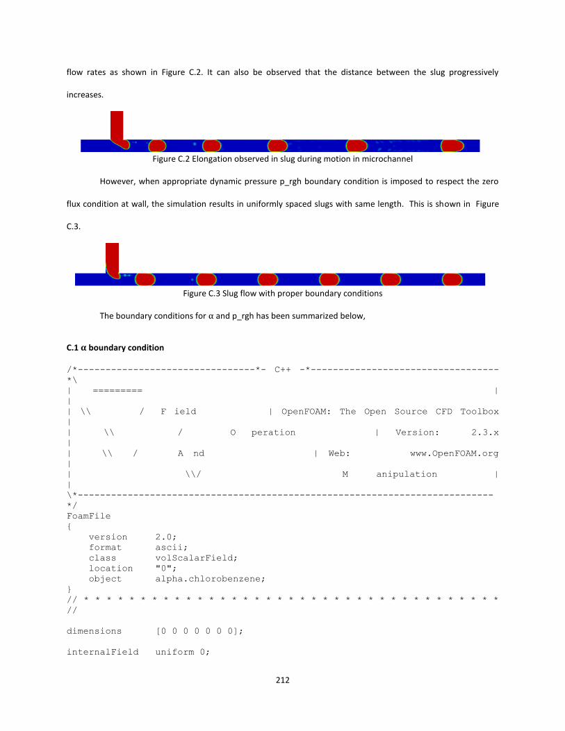
212

flow rates as shown in Figure C.2. It can also be observed that the distance between the slug progressively

increases.

Figure C.2 Elongation observed in slug during motion in microchannel

However, when appropriate dynamic pressure p_rgh boundary condition is imposed to respect the zero

flux condition at wall, the simulation results in uniformly spaced slugs with same length. This is shown in Figure

C.3.

Figure C.3 Slug flow with proper boundary conditions

The boundary conditions for and p_rgh has been summarized below,

C.1 boundary condition

/*--------------------------------*- C++ -*----------------------------------

*\

| ========= |

|

| \\ / F ield | OpenFOAM: The Open Source CFD Toolbox

|

| \\ / O peration | Version: 2.3.x

|

| \\ / A nd | Web: www.OpenFOAM.org

|

| \\/ M anipulation |

|

\*---------------------------------------------------------------------------

*/

FoamFile

{

version 2.0;

format ascii;

class volScalarField;

location "0";

object alpha.chlorobenzene;

}

// * * * * * * * * * * * * * * * * * * * * * * * * * * * * * * * * * * * * *

//

dimensions [0 0 0 0 0 0 0];

internalField uniform 0;

213

boundaryField

{

junction_wall

{

type constantAlphaContactAngle;

theta0 180;

limit gradient;

value uniform 0;

}

continuous_inlet_wall

{

type constantAlphaContactAngle;

theta0 180;

limit gradient;

value uniform 0;

}

disp_inlet_wall

{

type constantAlphaContactAngle;

theta0 180;

limit gradient;

value uniform 0;

}

channel_wall

{

type constantAlphaContactAngle;

theta0 180;

limit gradient;

value uniform 0;

}

outlet

{

type zeroGradient;

}

continuous_inlet

{

type inletOutlet;

inletValue uniform 0;

value uniform 0;

}

dispersed_inlet

{

type inletOutlet;

inletValue uniform 1;

value uniform 1;

}

}

// *************************************************************************

//

214

C.2 p_rgh boundary condition

/*--------------------------------*- C++ -*----------------------------------

*\

| ========= |

|

| \\ / F ield | OpenFOAM: The Open Source CFD Toolbox

|

| \\ / O peration | Version: 2.3.0

|

| \\ / A nd | Web: www.OpenFOAM.org

|

| \\/ M anipulation |

\*---------------------------------------------------------------------------

*/

FoamFile

{

version 2.0;

format ascii;

class volScalarField;

object p_rgh;

}

// * * * * * * * * * * * * * * * * * * * * * * * * * * * * * * * * * * * * *

//

dimensions [1 -1 -2 0 0 0 0];

internalField uniform 0;

boundaryField

{

junction_wall

{

type fixedFluxPressure;

adjoint no;

}

continuous_inlet_wall

{

type fixedFluxPressure;

adjoint no;

}

disp_inlet_wall

{

type fixedFluxPressure;

adjoint no;

}

channel_wall

{

type fixedFluxPressure;

adjoint no;

}

outlet

{

type fixedValue;

value $internalField;

}

215

continuous_inlet

{

type zeroGradient;

}

dispersed_inlet

{

type zeroGradient;

}

}

// *************************************************************************

//

216

Appendix D Permissions

The figures appearing in the document, adopted from the literature sources, have been included after

seeking appropriate permissions from the concerned agencies/authors.

1. Figure 2.2

217

2. Figure 2.5a

218

3. Figure 2.5 b

219

4. Chapter 3

220

5. Chapter 4

221

6. Figure 6.5

222

7. Figure 6.7 and Figure 6.8

223

Vita

Abhijit Rao, was born in January, 1986, in Tirthahalli, Karnataka, India. He completed his Bachelor’s degree

in Chemical Engineering at Visvesvaraya Technological University, Belgaum, India, in June 2007. He worked with

Reliance Industries Ltd, India, from Aug 2007 to June 2010 , as a Process Engineer. After a brief stint in industry he

joined Louisiana State University in Fall 2010 to pursue Phd in Cain Department of Chemical Engineering. While

working towards his doctoral degree he received master’s degree in ay 2014 at S . Abhijit is a candidate to

receive hid Doctoral degree in December 2015.