american economic association - ucluctp39a/blundell_pashardes_weber_aer_1993.pdf · by richard...

American Economic Association

What do we Learn About Consumer Demand Patterns from Micro Data?Author(s): Richard Blundell, Panos Pashardes and Guglielmo WeberSource: The American Economic Review, Vol. 83, No. 3 (Jun., 1993), pp. 570-597Published by: American Economic AssociationStable URL: http://www.jstor.org/stable/2117534 .

Accessed: 11/01/2014 11:26

Your use of the JSTOR archive indicates your acceptance of the Terms & Conditions of Use, available at .http://www.jstor.org/page/info/about/policies/terms.jsp

.JSTOR is a not-for-profit service that helps scholars, researchers, and students discover, use, and build upon a wide range ofcontent in a trusted digital archive. We use information technology and tools to increase productivity and facilitate new formsof scholarship. For more information about JSTOR, please contact [email protected].

.

American Economic Association is collaborating with JSTOR to digitize, preserve and extend access to TheAmerican Economic Review.

http://www.jstor.org

This content downloaded from 80.192.51.99 on Sat, 11 Jan 2014 11:26:29 AMAll use subject to JSTOR Terms and Conditions

http://www.jstor.org/action/showPublisher?publisherCode=aea

http://www.jstor.org/stable/2117534?origin=JSTOR-pdf

http://www.jstor.org/page/info/about/policies/terms.jsp


What Do We Learn About Consumer Demand Patterns from Micro Data?

By RICHARD BLUNDELL, PANOS PASHARDES, AND GUGLIELMO WEBER*

The aim of this paper is to assess the importance of using micro-level data in the econometric analysis of consumer demand. To do this we utilize a time series of repeated cross sections covering some 4,000 households in each of 15 years. Employing a number of different aggregation procedures, we conclude that aggregate data alone are unlikely to produce reliable estimates of structural price and income coefficients. However, once certain "aggregation factors" as well as trend and seasonal components are included, an aggregate model is not necessarily outperformed across all demand equations in terms of forecasting ability. (JEL D12, C52, C31)

The purpose of this paper is to develop a complete consumer demand system based on a time series of individual household data and to use it to measure the biases introduced into the study of consumer demand behavior when aggregate data are used in place of the appropriate microeconomic data. We assess the suitability of aggregate data through the impact on income and price elasticities and by evaluating the ability of both micro- and aggregate-based models to forecast aggregate consumer demand. The biases, introduced by the use of aggregate data, depend upon the way that household characteristics interact with in-

come and price effects and on departures of demand systems from linearity. We explore the structure of microeconomic demand systems and the role of household characteristics in the behavior of consumer demand both for the light this may shed on the pattern of future demands and for the implications this behavior has for issues of aggregation.

Consumer demand patterns typically found in micro data sets vary considerably across households with different household characteristics and with different levels of income. We model this variability by making intercept and slope parameters in the budget-share equations of our demand system depend on household characteristics and by allowing for nonlinear total log- expenditure terms. In fact, in theory- consistent demand systems it is total expenditure rather than disposable income that is allocated across goods. We find that this general framework leads to a well- specified data-coherent demand system, which is a quadratic extension of the popular "almost ideal" model of Angus S. Deaton and John Muellbauer (1980). The micro- level estimates are shown to be sensitive to the treatment of endogeneity of total expenditure and to the specification of interaction terms with household characteristics. In ad- dition, this specification is also shown to possess many attractive features for the evaluation of aggregate models.

*Blundell: University College London, Gower Street, London WC1E 6BT, U.K., and The Institute for Fiscal Studies, 7 Ridgmount Street, London WC1E 7AE, U.K.; Pashardes: City University, Northampton Square, London EC1V OHB, U.K., and The Institute for Fiscal Studies; Weber: University College London and The Institute for Fiscal Studies. This is a substantially re- vised version of University College London Discussion Paper No. 89-18. We thank Paul Baker, Martin Brown- ing, Mick Keen, Arthur Lewbel, Costas Meghir, John Muellbauer, Pedro Neves, Hashem Pesaran, Tom Stoker, Ian Walker, Ken Wallis, and two anonymous referees for comments on earlier versions of this paper. Finance for this research, provided by the Economic and Social Research Council at the Institute for Fiscal Studies, is gratefully acknowledged. We also thank the Department of Employment for providing the Family Expenditure Survey data used in this study but stress that we are solely responsible for the analysis and interpretation of the data.

570



VOL. 83 NO. 3 BLUNDELL ETAL.: MICRO DATA AND CONSUMER DEMAND 571

The parameters estimated on individual household data can be used to evaluate price and budget elasticities for each household in the sample and to calculate sum- mary elasticity measures, comparable in principle to what can be obtained by working with aggregate data. Using our data (the British Family Expenditure Survey, 1970- 1984) we find evidence of systematic aggregation bias over the sample period, especially with regard to the measurement of income effects.

We also investigate the ability of our micro-level model and a similar model estimated on aggregate data to forecast aggregate budget shares over a 24-month postsample period. The aggregate model we adopt is estimated on the aggregated micro data from the same sample and, following Thomas M. Stoker (1986), includes some simple distribution measures as well as seasonal and trend components. It also adopts the flexible specification of income and price effects as indicated by the micro data. In an out-of-sample forecast comparison of aggregate share predictions, we show that for certain equations forecasts from the aggregate model can outperform a forecast based on aggregated micro predictions.

These findings are not surprising, for although the aggregate model neglects information on time-varying household characteristics and should therefore have worse forecasting performance, the inclusion of certain distributional measures can correct for aggregation bias. Moreover, the aggregate model explains the aggregate share directly. This latter point gives the aggregate model an advantage over the micro model in two distinct ways. First, the micro estimates assume an independent distribution of unobservable errors and thereby ignore any common components in the micro-level errors. To some extent this serves as another motivation for the inclusion of a large number of observable common characteristics in the micro model. Secondly, in order to generate an aggregate forecast of expenditure shares from the micro model a weighted sum of micro share forecasts is required, rather than a simple average. For example, the aggregate budget share of food is defined as the expenditure on food over

the budget (or the total of nondurable expenditure) and is not the simple average of individual households' budget shares. Since the weights are likely to be endogenous at the micro level, the calculation of an unbiased forecast for the aggregate share from the micro model is shown to require careful treatment.

In Section I of this paper we discuss theoretical and econometric issues underlying our chosen micro-level model. We develop the concept of aggregation factors which can be used to detect likely sources of aggregation bias, and we discuss some issues that arise in using the micro results for forecasting. Section II presents econometric estimates and statistical tests for the micro model. In Section III we assess the importance of aggregation bias and relate it to the time-variability of the aggregation factors. Section IV presents the results of our comparison of forecasting abilities, and Section V concludes the paper.

I. The Modeling Framework

A. The Specification of Individual Preferences

We begin by considering an appropriate framework for the specification of preferences at the microeconomic level. Our ob- jective is to model a broad set of nondurable commodities that are well recorded in our micro data source. To this end we characterize preferences such that, in each period t, household h makes decisions on how much to consume of these commodities conditional on various household characteristics and also conditional on the consumption levels of a second group of other (possibly less flexible) demands. This latter group contains housing, tobacco expenditures, some durables, and labor-market decisions which, together with household characteristics, we represent by z.

The goods we model directly (q) refer to food, clothing, services, fuel (household en- ergy), alcohol, transport, and other non- durables. Clearly the relative amounts consumed of these commodities may well depend on the consumption of the second group of goods. Indeed, it is unlikely that



572 THE AMERICAN ECONOMIC REVIEW JUNE 1993

the two "groups" are weakly separable in utility. Rather the second group acts much like demographic or locational variables af- fecting both the allocation of total expenditure to these goods and the marginal rate of substitution between them. As a result we define household utility over qh for household h in period t conditional on the set of demographic and other conditioning variables z h (see Martin J. Browning and Costas Meghir [1991] for a discussion of conditional demands and weak separability).

The household may wish to save or to borrow according to the way in which it evaluates present and future needs, and this determines how much expenditure to allo- cate to current consumption and in particular to goods qh. Expenditure allocated to these goods, denoted by mt, is the first stage in a two-stage allocation process, and we shall be allowing for the endogeneity of mt using the two-stage budgeting framework to suggest identifying instrumental variables.'

Letting qiht represent consumption of good in period t, if utility is weakly separable

across time then the allocation of expenditure to good i, conditional on z , may be expressed as

( l ) Pit qi= i (pt, Mhl; Z h ) (1) it

=

where f1 describes within-period preferences and pt is the n-vector of period-t prices. Under (conditional) intertemporal weak separability, once Mh is chosen each fi can be determined without reference to prices or incomes outside the period (Blundell and Ian Walker, 1986).

To describe individual household preferences we first abstract from differences in z h

and write the share of expenditure i in period t (out of mh) for household h as

L

(2) S ht = ai + b'(pt) + E bj(pt)gj(Xh)

j=l

where xt is real total expenditure, b'(pt), b'(pt),.. , b (pt) are zero homogeneous functions of prices and gj(x h) are known polynomials in total real expenditure. The form of (2) is sufficiently general to cover many of the popular forms for Engel curves and demand systems. In particular, those of Holbrook Working (1943), Conrad E. V. Leser (1963), Deaton and Muellbauer (1980), and subsequent generalizations are generated with polynomials in the logarithm of real expenditure such as those in William M. Gorman (1981). Household characteristics may enter in a variety of different ways, the exact specification of which is primarily an empirical issue. Nevertheless, the specification of such variables will have a bearing on the form of the corresponding aggregate relationship, as we shall document below.

If we let Mt represent aggregate total household expenditure (E'/ M h) and let Ah equal the total expenditure share for household h (mh/Mt), then the Auh-weighted sum of individual budget shares Sit generates the aggregate share sit exactly. This point pro- vides another motivation for choosing preferences of form (2), since the equivalent aggregate relationship has the form

(3) Sit = ati + bo(pt) L H

+ E bji(pt) E thtgj(Xh)

j=1 h=1

and estimation of the unknown parameters in ai, bb ... ., b' on aggregated data can pro- ceed provided EhtgJ(x ) can be constructed in each period t. Moreover, if the gj(xh) do not depend on unknown parameters, estimation is possible on aggregate time-series data alone. As a result the class of preferences that generate (2) has been popular in the analysis of aggregation as is documented by Gorman (1981). Indeed, Gorman shows that if such preferences are utilized then the integrability conditions of demand theory require that the n x L coefficient matrix formed by ai + bo b, ..., 4b will have a rank no higher than three (see also Dale W. Jorgenson et al., 1980; Lawrence J. Lau, 1982; Robert Russell, 1983; Arthur Lewbel, 1989; John Heineke and Michael Shefrin, 1990).

IThese may contain price, income, seasonal, and demographic variables, as well as macro variables bearing on intertemporal substitution (like real interest rates) and macroeconomic indicators reflecting changes in expectations (like the unemployment rates).




To illustrate these points more explicitly, consider the following quadratic extension to Deaton and Muellbauer's (1980) "almost ideal" model (QUAIDS) which as we shall see represents the observed behavior in our Family Expenditure Survey data quite ade- quately. In this model L = 2 and the gj's are simply polynomial logarithmic terms so that (2) may be written as

(4) sit = ai + bb(pt) + b'(pt)ln xt 2 + b(pt) (ln x )

where household superscripts have been omitted for simplicity. If we restrict the coefficients on ln xt and (ln xt)2 to be independent of prices, that is, b(p t) = fi and b'(pt) = Ai, then integrability, in particular, symmetry of the Slutsky matrix, requires Ai= =3iE; that is, the ratio of the coefficients on the income and squared terms in income must be the same for all commodities. In this case, (4) becomes

(5) Sit = ati + bo(pt) +B pI[n xt + e(In xt) 2

and reduces the rank of the coefficient matrix defined above to two. For models of this form the maximum rank under symmetry is two. As a result, a test of symmetry in this model additionally requires a test of Ai-- f3iE. The "almost ideal" model of Deaton and Muellbauer imposes the further restriction that ? = 0.

B. Individual Household Characteristics, Seasonal Factors,

and Aggregation

With household data we also need to allow household preferences to depend on characteristics. The specific form we adopt for individual household-h preferences explicitly allows for the effect of the characteristics z on the polynomial coefficients in (4). In particular we write

(6) sit = ahxi + Eyij In pjt

+ 3, In Xf h + A't (pn Xth)

where the a ih, ph, and A h parameters are

allowed to vary with the household-h characteristics and other conditioning variables. For example, we write

(7) ah = ao + EakZt + EkTkt k k

in which we have also added a set of variables Tkt that are purely deterministic time-dependent variables, like seasonal dummies and time trends. The parameters Ah" and 3ht are also allowed to vary in a similar fashion. Consistent aggregation pro- ceeds, as in (3), by computing A-weighted sums of all variables.

To illustrate the implications for aggregate analysis of these generalizations consider the simplification in which we write

(8) h = p3i + fDDht

it= A + A Dht

where Dht is simply a zero-one dummy representing, say, the presence of children in the household. In our empirical work we find a number of such interactions with the real expenditure terms to be significant. The consistently aggregated relationship may be written as

(9) Sit-ao + E eij In pjt + i In Xt i

+ E36kTkt + AiEkht ln(xt/X ) k h

+ E aik E[ht zkt k h

+ D /9Ettht Dht ln xh

h

+ Ai EIht(ln Xh)2 h

+ AD ht Dht(ln xt) h

where Xt = Ehx t/Ht is average total real expenditure (Ht is the number of households in period t) and Uht = mh/Mt iS each household's relative weight in expenditure terms. As before the aggregate sit, the /iht-

weighted sum of micro shares Sit, simply equals the share of aggregate expenditure on good i out of total aggregate expenditure Mt.




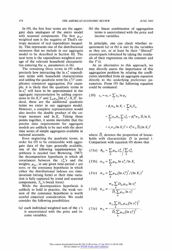
In (9), the first four terms are the aggregate data analogues of the micro model with seasonal components. The first aht- weighted sum is the negative of Theil's entropy measure of real expenditure inequality. This represents one of the distributional measures that we include in our aggregate model to be described in Section III. The next term is the expenditure-weighted average of the relevant household characteristics entering the ai parameters in (6).

The remaining three terms in (9) reflect precisely how interacting the ln x h expenditure terms with household characteristics and adding the quadratic term (ln xh)2 com- plicates consistent aggregation. For example, it is likely that the quadratic terms in ln xh will have to be approximated in the aggregate representation by adding expres- sions in (ln Xt)2 and EhAht[ln(xth/Xt)]2. In- deed, these are the additional quadratic terms we enter in our aggregate model. However, a complete representation would also involve the double product of the entropy measure and ln Xt. Taking these points together, it seems inevitable that the precise data requirements for aggregate models are unlikely to be met with the short time series of simple aggregates available in national accounts.

Even neglecting the quadratic terms, in order for (9) to be estimatable with aggregate data of the type generally available, one of the following supplementary hypotheses is needed (see Browning, 1987): the decomposition hypothesis in which all covariances between the Z4h s and the weights, PLht, in any given time-period t are zero; or the constancy hypothesis in which either the distributional indexes are time- invariant (strong form) or their time variation is fully captured by trend and seasonal components, Tkt's (weak form).

While the decomposition hypothesis is unlikely to hold in practice, the weak version of the constancy hypothesis is worth careful empirical consideration. We could consider the following possibilities:

(a) each individual weighted sum of the z's is uncorrelated with the price and income variables;

(b) the linear combination of aggregation terms is uncorrelated with the price and income variables.

In principle, one can check whether re- quirement (a) or (b) is met by the variables as they are, or at least by their "filtered" counterparts (obtained by taking the residuals of their regressions on the constant and the T's).

As an alternative to this approach, we may directly assess the importance of this aggregation problem by relating the coefficients identified from an aggregate equation directly to the underlying preference parameters. From (9) the following equation could be estimated:

(10) sit =o + yij In pjt J

+ I3iwot Iln Xt +? kTkt k

+ ~aikok(EZkt + i 72t Dt ln Xt k h

+ Ai7-1t(In Xt)2 + AD3t Dt(ln Xt)2

where Dt denotes the proportion of households with characteristic D in period t. Comparison with equation (9) shows that

(lla) OktZ=Ehtzkt/ E Zkt

(lc k1~t = 1: tthtlx ktln)

h h

( 1lb 70t = E: Iht l t /nX h

(llc '17t = EAht(In Xh

)2 I(n Xt)2 h

h v l t E Dht Aht Iln Xth

(~~~~ In Xe h

h




If the okt and -nj aggregation factors, (1 la)-(1 le), are approximately constant over time (with the rTj,'s close to unity), we may expect unbiased estimates from an aggregate equation like (10). If the wfjt's are constant and the okt are functions only of the deterministic time-dependent variables Tkt, the parameters of the "aggregate" model may still be stable and the yij's will be consistently estimated.

C. Econometric Analysis

The first issue we consider relates to the occurrence of zero expenditures in the diary records. For the commodity groups we consider, these will most likely correspond to purchase infrequency. The problem of infrequent expenditures has its major effect on goods like clothing, transport, and possibly alcohol (we do not consider tobacco consumption or expenditures on durable appliances in this paper). It means that the theoretical concept of "consumption" differs from its measured counter- part "expenditure." As this discrepancy affects both the dependent variable and the total-real-expenditure variable ln x', ordinary least-squares (OLS) estimates of the share equations are biased. However, instrumental-variable (IV) estimation (or more generally generalized method of moments [GMM] once heteroscedasticity is allowed for) permitting all terms in ln xh to be endogenous removes this measurement- error problem. As we wish to treat ln xh as endogenous, following the discussion above, we can use our IV or GMM estimates to obtain unrestricted consistent estimates for each equation. Homogeneity can also be checked at this stage since it is a within- equation restriction. Although each equation is estimated separately, adding-up and invariance are preserved for all of these linear estimators.

Turning to cross-equation restrictions, these can be imposed at a second stage using the minimum-chi-square (MCS) procedure (see Thomas Ferguson, 1958; Thomas J. Rothenberg, 1973). The attrac- tion of the MCS estimator for microecono- metric analysis of consumer behavior of the

type pursued here relates to the separate stages of imposing within- and cr6ss-equation restrictions.2 At the first stage, consistent estimates of the parameters of each equation with restrictions confined to within equations (zero-degree homogeneity in prices, for example) are recovered. For a standard demand system (linear expenditure system [LES] or "almost ideal" and its generalizations, for example), this would involve estimating separate linear share equations as described above. As we have also mentioned, in our case we allow for the endogeneity of all ln xh terms and of some other conditioning factors as well as considering the issue of general heteroscedasticity across households. These single-equation estimates together with their covariance matrix summarize all information available in the data concerning estimation of preference parameters. In effect they act as sufficient statistics for the purposes of demand-system estimation on the vast quantity of micro-level data. As a result the following second-stage restricted estimates attain asymptotic efficiency.

Denoting the vector of unrestricted parameters as +, cross-equation restrictions (symmetry, for example) on + may be expressed as

(12) g(

To impose these restrictions. the MCS method chooses an estimator +* so as to minimize the quadratic form

(13) (* = argmin[4 _g(+*)]', [4 g(+*)]

where 4 is the vector of unrestricted estimates and .,, is its estimated variance-

2For very large samples, this method can allow a considerable computational saving over the standard restricted-maximum-likelihood estimator since the di- mensions of the vector of unrestricted parameters can be significantly less than the number of observations.




covariance matrix.3 This procedure is adopted in the estimation of the restricted micro-level estimates to which we now turn.

II. The Micro Data Estimates

A. The Household Data

In this study we adopt the estimation procedure described in the previous section to recover estimates of a seven-good model of demand from a pooled cross section over 15 annual time series covering more than 61,000 households. These data are drawn from the annual British Family Expenditure Survey (FES) for the years 1970-1984. In one form or another the FES has been the cornerstone of many empirical studies of consumer behavior at the micro level, including, for example, the papers by Anthony B. Atkinson and Nicholas Stern (1980) and Robert A. Pollak and Terence J. Wales (1978). In our demand system we have concentrated on seven broad commodity groups: food, alcohol, fuel, clothing, transport, services, and other. In terms of sample selection, the results of the illustra- tion reported here refer to a sample of households whose head is more than 18 and less than 60 years of age and is not self- employed.4 Further details are provided in Appendix A.

B. The Estimated Models

We now turn to the estimated parameters and implied elasticities of the individual- household expenditure allocations. We present estimates from the quadratic extension of the "almost ideal" demand system in which second-order terms in ln xh are included as developed in Subsection I-B. In Table 1A the price and income coefficients that correspond to the yij, pi, and Ai parameters of share equations are presented; these correspond to equation (6). In all equations, we consistently find that both the own- and the cross-price parameters are statistically significant. It should be noted that all ln xh terms are treated as endogenous, and the restricted and unrestricted estimators are described in Subsection I-C, above.

Before considering the impact of household characteristics on the intercept terms ai in (6), we should stress that the coefficients on the logarithm of real expenditure terms, ln x and (ln x)2, are also found to display seasonal and demographic variation. In particular, there is a different budget response if there are children in the household (the interaction term C x ln x h between a child dummy and real expenditure has an important impact on alcohol, fuel, clothing, and services) and if the head of the household is a white-collar worker (e.g., see the coefficient on C x ln xh in the food, transport, and services equations).

Appendix B presents the complete estimation results for the first two equations (the others are omitted for space reasons but are available from the authors upon request). These tables document the household characteristics that were allowed to influence the ai intercept parameters in each share equation. Despite the large number of such characteristics, many of which have time variation, it is comforting to find that prices have a significant impact. The interpretation of the price parameters is probably best discussed in terms of elasticities, to which we turn below. However, the direct interpretation of the ai coefficients in each share equation is quite simple. For example the estimated coefficient

3The consistency of the resulting MCS estimator simply requires that the restrictions are correct and that + is a consistent estimator. Any positive-definite weight matrix can be used to replace ,- l However, where the correct weight matrix is used and where + is derived from an efficiency single equation technique, the MCS estimator is asymptotically equal to the maximum-likelihood estimator, and the minimized value of the quadratic form in (13) is an optimal chi-square test of the restrictions.

4We also selected out the tails of the income distribution. In particular, we looked at the sample distribution of the logarithm of real net income and discarded the observations in the bottom and top 1 percent. This selection (based on an econometrically exogenous variable) is meant to remove the possibility that small outliers in the income distribution are responsible for the nonlinearity in the budget-share equations.




on variable CH02 indicates that an additional child of less than three years of age will, ceteris paribus, add 0.01935 to the share of expenditure on food. On the other hand, with the head of the household being unemployed (HUNEMP), even allowing for income differences the ceteris paribus fall in the share is 0.01329. Large significant effects are found for car ownership and the number of cars (DCAR and CARS) even though they are allowed to be endogenous. The interpretation of characteristics in the other equations follows in the same fashion. As one might expect, the impact of these "taste-shifter" variables differs quite substantially across commodity groups.

The results from Table 1A appear to be plausible, and in Table 1B we present some formal statistical diagnostics. The overidentification tests are constructed under two assumptions. In the first row, homosce- dasticity is assumed, while in the second row this assumption is relaxed, and the GMM estimator proposed by Hal White (1982) is adopted. These results indicate two things: first, that the choice of instruments, described at the foot of Table 1B, is broadly valid; second, that adjusting for heteroscedasticity has little impact on the test statistics, suggesting that we have included sufficient household-specific interaction terms to account for heterogeneity in the error variances of the share equations.

A simple check for functional-form misspecification involves introducing a cubic term in ln xh in each equation and testing for its insignificance. A standard t test (reported in the third row of the table) con- firms that this extra nonlinearity is not needed. The test of the joint significance of the linear and quadratic ln xh terms, on the other hand, displays the distance the data stand from homotheticity or unitary income elasticities in which expenditure shares would be independent of total outlay.

In estimation, we treated all terms in ln xh and a number of household characteristics as endogenous and used instrumental variables. A formal exogeneity test can be constructed, and this strongly rejects the null hypothesis that our instrumental-variable estimates are insignificantly different

from ordinary least-squares ones. In fact, the test statistic (which is a x2 with 12 degrees of freedom under the null hypotheses) rejects even if we adopt the less strin- gent Schwarz criterion (Gideon Schwarz, 1978), which optimally adjusts the size of the test as the number of observations in- creases. The presence of simultaneity bias in OLS estimates is also confirmed by our out-of-sample forecasts to be presented below, in which we find systematic forecast errors from equations based on OLS parameters.

The homogeneity tests reported in Table 1B indicate that we were unable to reject the homogeneity restrictions implied by the theory, an issue which has proved to be a major stumbling block for other demand studies, especially with results on aggregate data (see e.g., Deaton and Muellbauer, 1980). The fact that here the price parameters are quite precisely estimated adds to the importance of our results. Moreover, both in the Deaton and Muellbauer (1980) study and in many that followed (e.g., Gordon Anderson and Blundell, 1982), dynamic misspecification is suggested as the root cause of homogeneity rejections. As was noted earlier, the omitted characteristics in aggregate models implied from this study may evolve in a way that is captured by the introduction of dynamic adjustment or trend-like terms, a point also noted by Stoker (1986).

Finally, in Table 1B we present the test statistics relating to the symmetry hypothesis. This is separated into two parts reflecting the discussion of Subsection 11-A. The first test statistic refers to the standard symmetry restriction on the yij parameters. Al- though the test statistic is high, a comparison of the unrestricted parameter estimates with the y-symmetry-constrained estimates of Table 1A indicates that very little is lost in imposing y-symmetry. Given symmetry on these price terms, we can turn to the second condition required for symmetry in the complete system which was shown in equation (5) to require proportionality between the parameters on the ln x terms and their corresponding (ln x)2 counterparts. Although the sign pattern in Table 1A ap-




TABLE 1-THE QUADRATIC ALMOST-IDEAL DEMAND SYSTEM

A. The yij, f3j, and Ai Coefficient Estimates:

Share equations

(i) (ii (iii) (iv) (v) (vi) Variable Food Alcohol Fuel Clothing Transport Services

Yii 0.1037 0.0188 - 0.0334 - 0.0231 - 0.0131 0.0034 (0.0126) (0.0084) (0.0074) (0.0125) (0.0147) (0.0102)

Yi2 0.0188 - 0.0434 0.0468 0.0103 0.0050 - 0.0063 (0.0084) (0.0108) (0.0070) (0.0100) (0.0134) (0.0101)

Yi3 - 0.0334 0.0468 0.0397 - 0.0040 - 0.0433 - 0.0292 (0.0074) (0.0070) (0.0086) (0.0091) (0.0107) (0.0079)

Yi4 - 0.0231 0.0103 - 0.0040 0.0376 - 0.0284 - 0.0386 (0.0125) (0.0100) (0.0091) (0.0179) (0.0174) (0.0119)

Yi5 - 0.0131 0.0050 - 0.0433 - 0.0284 0.0605 0.0266 (0.0147) (0.0134) (0.0107) (0.0174) (0.0317) (0.0169)

Yi6 0.0034 -0.0063 - 0.0292 - 0.0386 0.0266 0.0387 (0.0102) (0.0101) (0.0079) (0.0119) (0.0169) (0.0166)

pi - 0.0377 0.0891 - 0.4433 0.2940 - 0.1310 0.3829 (0.1301) (0.1066) (0.0758) (0.1389) (0.2058) (0.1481)

Ai - 0.0076 - 0.0017 0.0370 - 0.0264 0.0151 - 0.0273 (0.0112) (0.0092) (0.0065) (0.0120) (0.0178) (0.0128)

i(S3) 0.0561 0.1486 0.1561 -0.1383 -0.1299 - 0.0758 (0.0866) (0.0705) (0.0492) (0.0922) (0.1366) (0.0975)

Aj(S3) - 0.0053 - 0.0134 - 0.0123 0.0113 0.0111 0.0071 (0.0070) (0.0060) (0.0042) (0.0079) (0.0118) (0.0084)

Pi(C) -0.0038 -0.0466 0.0386 -0.0297 -0.0009 0.0501 (0.0122) (0.0100) (0.0070) (0.0130) (0.0193) (0.0138)

Ai(C) 0.0000 0.0060 -0.0054 0.0051 -0.0015 -0.0057 (0.0016) (0.0013) (0.0009) (0.0017) (0.0025) (0.0018)

/3j(WHC) 0.4024 0.0670 0.0190 - 0.1053 - 0.6504 0.4223 (0.1436) (0.1177) (0.0830) (0.1564) (0.2263) (0.1614)

Aj(WHC) - 0.0349 - 0.0041 - 0.0005 0.0074 0.0548 - 0.0356 (0.0124) (0.0101) (0.0071) (0.0135) (0.0195) (0.0639)

pears broadly to support this proportionality, the test statistic strongly rejects, and in our evaluation of the properties of this model we have decided not to present results with this restriction imposed.

C. Price Aggregation

In Table 2 we investigate the joint significance of the price terms by comparing a model with all prices included to one in which the deflated own price only is included. From the chi-square tests of the

joint significance of the extra terms (A. Ronald Gallant and Jorgenson, 1979), it is clear that the cross-price terms are important.

D. Model Elasticities

Inspection of the parameter estimates for the estimated demand models reveals some general patterns. For example, services are a luxury while fuel is a necessity. Each household h will, however, have a different budget elasticity. In the context of the




TABLE 1-Continued.

B. Test Statistics for Quadratic Almost-Ideal System:

Share equations

Test Food Alcohol Fuel Clothing Transport Other Services

Overidentification 50.65 54.75 110.86 58.41 37.54 27.98 33.95 simple IV, X[21

Overidentification 50.01 56.74 106.71 58.36 37.00 28.71 33.52 White IV, X1217]

Functional form, - 0.043 2.319 1.772 - 0.730 - 0.863 - 0.999 0.493 -t value

ln Xh terms, X[2] 23.20 153.12 117.52 37.21 63.76 34.72 160.30

(Swz = 88.27) Exogeneity (Wu- 285.84 628.56 391.68 147.24 602.40 66.69 251.28

Hausman) X12 (Swz = 132.41K

Homogeneity, 0.066 0.163 0.755 - 0.581 - 0.388 - 0.095 0.597 t value

Symmetry: = y11, X[2] = 54.0364

A1 = 203 , X[2Q]= 115.9694

Notes: Standard errors are given in parentheses; y-symmetry constrained the estimates. Variables treated as endogenous in estimation: ln x,(ln x)2, C x ln x, C x (ln x)2, WHC x In x, WHC x (ln x)2, S3 x ln x, S3 x (ln x)2, DTOB ( = 1 if there is a smoker in the household), CTOB, DCAR, and CARS (see Appendix A for further definitions). Instruments not included in the equation: professional, managerial, and teacher dummies, current and lagged durable prices, current prices of "other" and housing, lagged transport price, trending seasonals, lagged unemployment rates (1 and 12 months previous), lagged real lending and borrowing rates, net normal income (ln Y),S1 x ln Y,S2x ln Y,S3 xln Y,(lnY)2, C x ln Y,C x(ln Y)2,WHCxln Y,WHCx (ln Y)2,S3 x(ln y)2, dummy for three-day week (1974:1), C x(age), C x(age)2, and (trend)2. Swz is the critical value of the test statistic based on the Schwarz criterion.

quadratic model estimated above at reference prices this elasticity is defined as

(14) ei = (PP+ 2A'j In mh)/si + 1.

As documented above our empirical specification allowed ,3ih and A,V to vary with family composition and the occupation of the household head. Moreover, the budget elasticity is likely to exhibit substantial variation between households because it de- pends on the level of the budget itself. Also, as we can see from the impact of the many included characteristics, the predicted expenditure share s h will vary across households. This variation of elasticities across the sample is a distinct advantage of using individual household-level data across time

rather than aggregate time series, where often only a single elasticity estimate for all households in any period is given.

The uncompensated elasticity of good i with respect to the price of good j is given by

(15) e,hj=(Yijsih)

- (f + 2Ah' in mh) ( s/s ) -kij

where kij = 1 if i= j and kij = O if i j. The compensated price elasticity is simply

(16) eh = eh + e hSh

Both (15) and (16) take into account the




TABLE 2-RESTRICTIONS ON CROSS-PRICE PARAMETERS

Commodity

Term Food Alcohol Fuel Clothing Transport Other Services

A. Unrestricted:

Food 0.106 0.029 -0.015 -0.057 0.013 -0.065 -0.011 (0.017) (0.013) (0.009) (0.017) (0.026) (0.012) (0.018)

Alcohol - 0.059 -0.029 0.039 0.009 0.059 - 0.036 0.018 (0.017) (0.014) (0.010) (0.018) (0.027) (0.013) (0.019)

Fuel - 0.040 0.038 0.047 - 0.025 - 0.039 0.009 0.011 (0.017) (0.013) (0.009) (0.017) (0.026) (0.012) (0.019)

Clothing 0.037 - 0.003 - 0.013 0.054 - 0.039 0.052 - 0.016 (0.022) (0.018) (0.012) (0.023) (0.035) (0.016) (0.025)

Transport -0.093 0.006 -0.058 -0.013 0.118 -0.008 0.048 (0.025) (0.020) (0.014) (0.026) (0.038) (0.019) (0.027)

Services 0.038 - 0.009 - 0.040 - 0.019 0.002 0.018 0.010 (0.017) (0.014) (0.010) (0.018) (0.027) (0.013) (0.019)

ln x -0.021 0.057 - 0.302 0.177 - 0.026 - 0.082 0.196 (0.083) (0.068) (0.047) (0.088) (0.131) (0.061) (0.094)

(ln x)2 -0.017 0.000 0.037 - 0.025 0.012 0.007 -0.015 (0.011) (0.009) (0.006) (0.012) (0.018) (0.008) (0.013)

C x ln x - 0.006 - 0.057 0.045 - 0.027 - 0.013 - 0.005 0.063 (0.015) (0.012) (0.009) (0.016) (0.024) (0.011) (0.017)

C x(ln X)2 0.001 0.011 -0.009 0.007 -0.000 0.002 -0.011 (0.002) (0.002) (0.002) (0.003) (0.002) (0.002) (0.003)

B. Grouping Restrictions:

Own price 0.127 -0.035 0.073 0.028 0.012 0.026 0.054 (0.011) (0.009) (0.007) (0.013) (0.035) (0.014) (0.018)

ln x - 0.095 0.113 - 0.354 0.137 -0.140 -0.102 0.194 (0.080) (0.063) (0.047) (0.084) (0.130) (0.057) (0.089)

(In x)2 - 0.005 -0.007 0.043 - 0.020 0.024 0.011 -0.018 (0.011) (0.009) (0.006) (0.011) (0.018) (0.008) (0.012)

C xln x - 0.011 - 0.052 0.045 -0.031 - 0.014 - 0.009 0.066 (0.015) (0.012) (0.009) (0.016) (0.024) (0.011) (0.17)

C x(ln X)2 0.001 0.010 -0.009 0.008 -0.000 0.003 -0.011 (0.002) (0.002) (0.002) (0.003) (0.005) (0.002) (0.003)

Share: 0.348 0.067 0.085 0.102 0.178 0.103 0.117 GJ(5): 11.04 20.80 104.90 28.48 14.44 34.12 6.19

Notes: Standard errors are given in parentheses. The retail price index for these components is used as a general deflator throughout. GJ(5) is the test statistic from x2 tests of the joint significance of the extra terms (Gallant and Jorgenson, 1979).




TABLE 3-PRICE AND BUDGET ELASTICITIES

A. Budget Elasticities Computed at the Average Shares and Household Characteristics:

Commodity

Estimator Food Alcohol Fuel Clothing Transport Services

GMM 0.608 2.290 0.838 0.917 1.201 1.448 (0.07) (0.28) (0.15) (0.24) (0.20) (0.22)

OLS 0.574 1.290 0.409 1.994 1.329 1.207 (0.01) (0.04) (0.02) (0.03) (0.02) (0.03)

B. Compensated Price Elasticities:

Commodity

Commodity Food Alcohol Fuel Clothing Transport Services

Food -0.354 0.122 -0.012 0.034 0.141 0.128 (0.04) (0.02) (0.02) (0.04) (0.04) (0.03)

Alcohol 0.627 -1.582 0.785 0.255 0.254 0.024 (0.13) (0.16) (0.11) (0.15) (0.20) (0.15)

Fuel - 0.048 0.618 - 0.448 0.054 - 0.331 - 0.226 (0.09) (0.08) (0.10) (0.11) (0.13) (0.09)

Clothing 0.116 0.169 0.045 -0.526 -0.103 -0.264 (0.12) (0.10) (0.09) (0.18) (0.17) (0.12)

Transport 0.271 0.095 -0.157 - 0.058 - 0.483 0.267 (0.08) (0.08) (0.06) (0.10) (0.18) (0.09)

Services 0.375 0.013 -0.162 -0.226 0.405 - 0.554 (0.09) (0.09) (0.07) (0.10) (0.27) (0.14)

OLS compensated own-price elasticities: - 0.429 - 1.537 -0.445 - 0.686 - 0.488 -0.667 (0.04) (0.16) (0.10) (0.17) (0.17) (0.13)

C. Uncompensated Price Elasticities:

Commodity


Food - 0.564 0.081 - 0.064 - 0.028 0.032 0.056 (0.04) (0.02) (0.02) (0.04) (0.05) (0.03)

Alcohol -0.163 -1.735 0.590 0.024 -0.156 -0.247 (0.17) (0.16) (0.11) (0.15) (0.22) (0.16)

Fuel - 0.337 0.562 -0.519 -0.031 -0.481 - 0.325 (0.13) (0.09) (0.10) (0.11) (0.15) (0.10)

Clothing - 0.200 0.108 - 0.033 -0.619 - 0.267 - 0.372 (0.14) (0.10) (0.09) (0.18) (0.18) (0.12)

Transport -0.143 0.015 -0.259 -0.179 - 0.698 0.125 (0.10) (0.08) (0.06) (0.10) (0.19) (0.10)

Services - 0.125 - 0.084 - 0.286 - 0.372 0.146 - 0.725 (0.11) (0.09) (0.07) (0.10) (0.28) (0.14)




TABLE 3- Continued.

D. Distribution of Uncompensated Own-Price Elasticities by Total Expenditure:

Expenditure Commodity group Food Alcohol Fuel Clothing Transport Services

Low 5 percent - 0.671 -1.79 -0.680 -0.468 -0.553 -0.667 (0.017) (0.095) (0.020) (0.070) (0.161) (0.079)

6-10 percent -0.647 -1.72 -0.641 -0.554 -0.561 -0.731 (0.023) (0.093) (0.034) (0.065) (0.191) (0.076)

11-25 percent - 0.622 -1.65 -0.599 -0.581 -0.615 -0.721 (0.018) (0.053) (0.027) (0.036) (0.104) (0.056)

Middle 50 - 0.556 - 1.57 - 0.486 - 0.625 - 0.727 - 0.737 percent (0.020) (0.037) (0.026) (0.020) (0.051) (0.030)

76-90 percent - 0.472 - 1.53 - 0.369 - 0.642 - 0.810 - 0.739 (0.070) (0.101) (0.082) (0.051) (0.093) (0.057)

Top 10 percent - 0.324 -1.48 -0.425 - 0.626 -0.925 -0.712 (0.239) (0.149) (0.159) (0.103) (0.149) (0.094)

All - 0.514 -1.55 - 0.479 - 0.625 - 0.798 - 0.729 (0.033) (0.031) (0.025) (0.018) (0.042) (0.022)

E. Distribution of Budget Elasticities by Total Expenditure.

Expenditure Commodity group Food Alcohol Fuel Clothing Transport Services

Low 5 percent 0.788 2.378 0.510 1.470 0.762 2.598 (0.032) (0.206) (0.034) (0.118) (0.192) (0.315)

6-10 percent 0.752 2.251 0.545 1.235 0.904 2.146 (0.030) (0.206) (0.045) (0.089) (0.148) (0.239)

11-25 percent 0.708 2.118 0.610 1.114 1.041 1.867 (0.021) (0.113) (0.029) (0.048) (0.061) (0.130)

Middle 50 0.591 1.947 0.852 0.913 1.209 1.371 percent (0.030) (0.079) (0.031) (0.031) (0.039) (0.048)

76-90 percent 0.424 1.859 1.296 0.758 1.355 1.038 (0.128) (0.226) (0.100) (0.088) (0.143) (0.075)

Top 10 percent 0.096 1.736 1.829 0.602 1.478 0.722 (0.549) (0.328) (0.228) (0.235) (0.310) (0.290)

All 0.501 1.884 1.057 0.822 1.310 1.162 (0.069) (0.069) (0.050) (0.037) (0.052) (0.066)

Note: Numbers in parentheses are standard errors.

Stone-index approximation for the total expenditure deflator In P = Yish n pi and exhibit variation between households.

Table 3A-C reports the elasticities as defined above computed at the average shares and household characteristics. A

comparison with the OLS row displays the importance of allowing for endogeneity in the total-expenditure terms. In the matrix of compensated price elasticities (Table 3B), it can be observed that own-price effects are large and negative while the cross-price ef-




fects are generally positive. Moreover, all the eigenvalues of the Slutsky matrix (evaluated at mean expenditure levels) were found to be negative. This shows a close adherence to concavity and taken together with the above results suggests, perhaps sur- prisingly, that integrability conditions are not too much at odds with observed micro behavior.

To illustrate the variation of elasticities across households, parts D and E of Table 3 report the uncompensated own-price and budget elasticities for households grouped by total expenditure. An interesting result in this table is the budget elasticity reversal in the case of several goods. In some cases this may reflect genuine changes in the per- ception of need at different income levels; for example, clothing is perceived to be a luxury at low income and a necessity at high income. In other cases it may reflect changes in the type of good consumed at different income levels; for example, the elasticity reversal of demand for transport probably reflects demand for public transport (a necessity) by the poor as opposed to demand for private motoring (a luxury) by the rich. The differences in the budget elasticities in Table 3E are reflected in the variation of the uncompensated own-price elasticities in the first part of the same table.

III. An Empirical Evaluation of Aggregation Bias

As was noted in the discussion of aggregation bias in Section I, the empirical model estimated on micro data does not lend itself to the simplest forms of aggregation for two reasons. First there are the quadratic terms in the logarithm of real expenditure, and second there are interaction terms between the demographic variables and the real expenditure terms. It is however possible to assess the type of results that would emerge if an empirical investigator tried to estimate share equations for the relevant groups of commodities on aggregate data.

A first possibility for our hypothetical investigator would be to follow the aggregation procedure described by equation (9) in Subsection I-B and appropriately weight all

right-hand-side variables by the share of individual total expenditure in aggregate total expenditure. Given the large number of interaction terms in the micro model, this approach would generally be ruled out by a lack of degrees of freedom in the aggregate model. Even if a guide to which variables would be important in the aggregate model were possible, it is unlikely that such exactly aggregated variables would be available over the complete time series. As a result we adopt a more parsimonious option in which household characteristics are ignored, and each budget share is regressed on the logarithm of prices, the log of average real expenditure and its squared term, seasonal components, trend terms, and the simple linear and quadratic entropy distribution measures to capture the basic aggregation effects also described in the discussion of equation (9) above.

This analysis utilizes aggregated monthly Family Expenditure Survey data over the exact same time period as used in the micro analysis. We include monthly time dummies which together with the price terms, the total expenditure terms, the two entropy measures of distributional change, a tem- perature measure, and a trend term result in 23 explanatory factors for each aggregate expenditure share equation. In contrast to the micro model the corresponding exogeneity test suggested little need to account for the potential endogeneity of ln x terms. As a result, the aggregate demand system is estimated using the standard seemingly un- related regressions estimator on the constructed monthly time-series data base, and it is these results that we present in what follows.

Although the entropy measures, the trend terms, and the seasonal components are included, it is impossible to include all terms suggested by the micro model. However, it is interesting to ask whether the omitted factors in this aggregate model induce any dynamic misspecification and if so whether it is sufficient to invalidate the homogeneity hypothesis. To address the issue of dynamic misspecifications we calculated the LM test of autocorrelation. The test assesses the importance of misspecification over own and




TABLE 4-ELASTICITIES FROM THE AGGREGATE MODEL

A. Budget Elasticities:

Commodity


GMM 0.547 0.621 0.569 0.903 1.855 1.806 (0.13) (0.42) (0.31) (0.43) (0.40) (0.53)

B. Compensated Price Elasticities:

Commodity


Food -0.417 0.063 0.034 0.040 0.148 0.162 (0.05) (0.03) (0.03) (0.05) (0.06) (0.05)

Alcohol 0.322 -1.260 0.482 0.352 0.697 -0.132 (0.17) (0.20) (0.15) (0.18) (0.25) (0.19)

Fuel 0.136 0.380 -0.492 0.057 -0.293 -0.014 (0.13) (0.12) (0.15) (0.14) (0.18) (0.13)

Clothing 0.963 -0.349 -0.359 - 1.107 0.346 0.081 (0.16) (0.12) (0.12) (0.20) (0.20) (0.15)

Transport 0.754 0.087 0.071 0.035 - 0.871 0.116 (0.12) (0.09) (0.09) (0.11) (0.25) (0.15)

Services 0.706 0.155 0.124 0.267 0.124 -0.906 (0.13) (0.11) (0.10) (0.13) (0.05) (0.03)

C. Uncompensated Price Elasticities:

Commodity


Food -0.605 0.026 -0.013 -0.015 0.050 0.098 (0.08) (0.03) (0.03) (0.05) (0.08) (0.05)

Alcohol 0.108 -1.301 0.429 0.289 0.585 -0.206 (0.31) (0.21) (0.15) (0.19) (0.33) (0.23)

Fuel - 0.060 0.341 - 0.540 0.000 - 0.395 - 0.081 (0.24) (0.12) (0.15) (0.15) (0.25) (0.17)

Clothing 0.651 -0.409 -0.436 - 1.198 0.184 -0.026 (0.20) (0.11) (0.12) (0.19) (0.22) (0.16)

Transport 0.115 -0.038 -0.087 -0.152 -1.203 -0.103 (0.14) (0.09) (0.09) (0.12) (0.26) (0.16)

Services 0.083 0.034 -0.030 0.085 -0.199 - 1.119 (0.17) (0.11) (0.10) (0.13) (0.12) (0.07)

D. Budget-Elasticity Differences Between Micro and Aggregate Models:

Commodity


GMM - 0.003 1.353 0.372 -0.683 -0.090 -0.149 (0.04) (4.37) (2.04) (2.46) (0.37) (0.51)




TABLE 4- Continued.

E. Compensated-Price Elasticity Differences Between Micro and Aggregate Models:

Commodity


Food 0.074 0.050 - 0.040 - 0.056 0.022 - 0.020 (1.16) (0.98) (0.92) (0.65) (0.14) (0.19)

Alcohol 0.255 - 0.293 0.269 - 0.076 - 0.407 0.146 (0.65) (1.31) (1.19) (0.17) (0.50) (0.27)

Fuel -0.161 0.212 0.070 -0.069 -0.064 -0.156 (0.53) (1.11) (0.50) (0.20) (0.10) (0.37)

Clothing -0.192 -0.051 - 0.058 -0.054 0.105 0.083 (0.72) (0.28) (0.35) (0.27) (0.19) (0.23)

Transport 0.042 - 0.152 - 0.030 0.059 - 0.060 0.064 (0.27) (1.58) (0.35) (0.35) (0.26) (0.30)

Services - 0.060 0.082 - 0.112 0.071 0.098 - 0.023 (0.26) (0.62) (0.87) (0.28) (0.20) (0.09)

Chi-square values for joint tests: Compensated price elasticities: 14.66 [d.f. = 21] Budget elasticities: 29.66 [d.f. = 6]

Notes: Numbers in parentheses are standard errors in parts A-C and t statistics in parts D and E.

cross autocorrelation in the error terms at first, third, and twelfth orders. Only in fuel and transport was there an indication of dynamic misspecification. Moreover the aggregate model did not reject price homogeneity.

For policy purposes it may be more useful to compare elasticities. Parts A-C of Table 4 provide the aggregate model elasticities evaluated at the sample means. Parts D and E compare these with the elasticities obtained directly from micro data reported in Table 3 by presenting their differences and the t values associated with these differences. The joint chi-square test for budget elasticities indicates a rejection of equality. Interestingly there is less evidence of bias in the price elasticities, although some differences are relatively large. However, given that relative prices are only time-varying and given that the aggregate model includes seasonals, trend, and entropy terms, this may not be surprising.

It is hard to predict circumstances under which the estimated price and income effects from the aggregate models will give a

reliable picture of the underlying microeconomic behavior. Some guidance on this topic may come from looking at the ratios of ,A-weighted averages to simple averages of the explanatory variables used in the micro level. These correspond to the ok aggregation factors in the consistently aggregated model (10) of Section I. Those variables for which the ratios are uncorrelated with prices and income do not require direct inclusion in the aggregate model. If their simple averages over time are either constant, or trend-like, they can be omitted altogether.

Table 5 presents selected results of regressions of some O's on trend, prices, and real expenditure, which confirm that the simple demographic variables may cause major problems in identifying price and especially income effects from aggregated data alone. The column headed CH1116, representing the effect of older children aged 11-16, shows that, for some demographic characteristics, the ratio of ,-weighted average to simple average is fairly constant. However, in all other cases considered there are nonnegligible correlations with price




TABLE 5-REGRESSION OF SELECTED ok'S ON PRICES AND REAL EXPENDITURE

0

Variable CH1116 (AGE)2 ADLTNR WHC YORK OWNER DCAR

PFOOD 0.047 0.141 0.105 -0.007 0.019 -0.854 -0.037 (0.207) (0.103) (0.094) (0.162) (0.344) (0.139) (0.072)

PALCL -0.030 0.109 0.092 0.681 0.519 0.202 0.190 (0.205) (0.102) (0.093) (0.160) (0.341) (0.138) (0.071)

PFUEL -0.018 0.014 -0.283 -0.040 0.289 -0.175 -0.163 (0.197) (0.098) (0.089) (0.154) (0.328) (0.132) (0.069)

PCLOTH 0.080 - 0.053 -0.148 - 0.047 0.555 -0.021 - 0.037 (0.257) (0.128) (0.116) (0.200) (0.427) (0.172) (0.089)

PTRPT -0.069 0.083 -0.018 0.166 1.150 0.164 -0.133 (0.281) (0.141) (0.128) (0.219) (0.468) (0.189) (0.098)

PSERV -0.000 -0.150 0.129 -0.333 -1.203 0.019 0.042 (0.204) (0.102) (0.093) (0.159) (0.340) (0.137) (0.071)

In x -1.819 2.151 -1.316 0.003 3.451 -3.018 -2.321 (1.593) (0.795) (0.721) (1.242) (2.647) (1.069) (0.553)

(In x)2 0.138 -0.164 0.101 0.002 -0.271 0.229 0.177 (0.122) (0.061) (0.055) (0.095) (0.202) (0.082) (0.042)

Mean: 1.175 0.919 1.181 1.128 0.931 1.107 1.133 R2: 0.206 0.114 0.227 0.393 0.160 0.241 0.330 DW: 1.863 1.878 2.001 2.057 2.150 1.908 1.907

Notes: Monthly regressions over 15 years. All regressions include an intercept, a time trend, and 11 monthly dummies. Standard errors are given in parentheses. See Appendix A for definitions of variables. DW is the Durbin-Watson statistic.

(e.g., see the ADLTNR equation) and expenditure terms., particularly in the case of home owners (OWNER).

The case of the coefficients on the real expenditure terms is more complex. As our analysis in Section I revealed, consistent parameter estimates of these coefficients can be obtained only if the wr aggregation factors of equations (llb)-(lle) are constant and close to unity. By their nature, the 7T's are unlikely to be unity. For example, wr0 is the ratio of the weighted average of ln x to the logarithm of the simple average of real expenditure. As the weights are given by an increasing function of ln x, this ratio will typically exceed 1. The same applies for wr1 (involving the square of real expenditure). The case is less clear-cut for the w2 and 773

ratios, which include demographic-related characteristics (households with children and households whose head is a white-collar worker). In this case, wr is the ratio of the (weighted) average of the product to the

product of the (weighted) averages. It will exceed 1 if the demographic characteristic in question is positively correlated with total real expenditure.5

Figure 1 presents graphs of the variations of the iTO and w2 ratios over time (wT relates to presence of children, 7T' to

5This statement needs qualifying though. From equation (11),

7VO =: E h In Xh /In X h

( Ehhlnhx I H-lEhlnxh I

H lEh In xh ln(Ehxh/H) )

where H is the total number of households. In the text, we argued that the first ratio is at least 1; however, Jensen's inequality implies that the second will be 1 at most. In practice, the second ratio is fairly stable and close to unity.




1.20

OG. 1. 10 -," - - vr if2

1.05 ITro

1970 1975 1980 1985

FIGURE 1. AGGREGATION FACTORS:

TERMS INVOLVING ln( x)

white-collar workers). Since these aggregation factors are not dependent on any estimated parameters, this figure not only cov- ers the within-period sample but also 24 months of postsample information which will be used for a forecast comparison in the next section. It clearly shows that only in the case of rro is there limited variability. In practice, we could take a given value of rro and use it to scale down parameter estimates obtained using aggregate data. Whenever the 7T's are time-varying the estimated parameters in the aggregate model are likely to be unstable. It appears that this will occur for all the other expenditure terms. This is particularly systematic for the interaction between ln x and the white- collar dummy. The time-series variation of 7r'w suggests that there has been high positive correlation between being a white-collar worker and overall expenditure in the early 1970's and early 1980's, and a much lower one in the mid-to-late 1970's.

In Figure 2 the aggregation factors relating to (ln X)2 (i.e., rT, and 7T3) are presented. Again the white-collar worker variable, 7T s, shows systematic time-series variation. Together these results indicate that differences in the distribution of expenditures between and across households of different types can lead to systematic time variation in aggregate model parameters. It is worth noting, however, that there is less variation in the postsample period, which may make it less likely that any systematic instability will be observed over this period.

1.3 - - 1T3

O 1.2 -

Y ~ ~ ~ \ _

, l l X , , W , 1 1

IT1

1970 1975 1980 1985

FIGURE 2. AGGREGATION FACTORS:

TERMS INVOLVING ln(x) SQUARED

With this in mind we turn, in the next section, to the comparison of forecasts of aggregate shares from an aggregate model to those generated from the (weighted) sum of micro model forecasts over this period.

IV. Forecast Performance

In assessing the forecast performance of the micro and aggregate specifications we are naturally drawn to compare postsample predictions of aggregate behavior. As we noted earlier there are likely to be factors that mitigate the efficiency and bias consid- erations derived in the previous section when aggregate forecast performance is compared. First, the micro model, in assum- ing independent variation in unobservable factors across households, will not necessarily produce the best fit in the time-series domain. Second, since weighted summation is required to calculate the aggregate share and since the weights are most likely endogenous, one has to be careful to remove any resulting bias at the summation stage. Finally, our aggregate model described in Section III is estimated on the aggregated micro data and includes distribution, trend, and seasonal components to minimize aggregation bias.

Since our estimation period ends in 1984, we decided to consider out-of-sample forecast performance for the 24 months in the 1985 and 1986 Family Expenditure Survey data. In line with Section II, we also decided to maintain use of the instrumental-




0.02-

0o A. At :

--; IV eors-mcro OLS errors-micro V

-0.04 I, I,I,,,i,,, 1,

Jan Jul Jan Jul 1985 1985 1986 1986

FIGURE 3. ESTIMATOR FORECAST PERFORMANCE:

MICRO TRANSPORT SHARE EQUATION

0.02 A ,A

I i.~~~~~~~~~~ co

0 ,

-0.02 I X

-IV effors -macro OLS errors-macro

-0.04 I I I ., I I i I I I I Jan Jul Jan Jul 1985 1985 1986 1986

FIGURE 4. ESTIMATOR FORECAST PERFORMANCE:

MACRO (AGGREGATE) TRANSPORT SHARE EQUATION

variable (GMM) estimated micro system. Figure 3 uses the transport equation as an example of the persistent bias over the forecast period that is present in the micro OLS estimates. The other micro equations display a bias of similar magnitudes. For the aggregate model, this bias is less evident. In Figure 4 the corresponding forecast error for the transport equation is reported and supports our view that the standard OLS estimator should be used for the aggregate model. As we noted above in comparison

with the micro model, the within-sample exogeneity test statistics are small.

The comparative precision in forecast performance is presented in Table 6. We turn first to the mean forecast error over the 24-month period. The individual household forecasts have to allow for the endogeneity of the ln x terms and the ,Lu weights. To account for the endogeneity of terms in ln x we include the estimated reduced-form residuals, which is equivalent to forecasting with the structural restrictions imposed. Note however that to construct the forecast of the aggregate share the a-weighted sum is required. Since this sum includes the weighted sum of micro error terms, the forecast will only be unbiased if the error terms are uncorrelated with the weights. However, since _h = Xh/X , accounting for the endogeneity of the terms in ln x and (ln X)2 as described above all but purges the correlation between the error terms and the /,t weights.

Table 6A shows the close accordance of the forecasts from the two models. This is further displayed in Figures 5-11, where the monthly forecast errors are presented. On these aggregate monthly data the micro model does not always dominate, only out- performing the aggregate model for clothing, transport, "other" goods, and services. This pattern is confirmed when the postsample (Table 6B) and the within-sample root-mean-square-error criteria (Table 6C) are computed.

One further comparison is also useful. As we pointed out in the Introduction, the aggregate model has an apparent built-in advantage, in that it works directly with ,u- weighted shares. One way to evaluate the empirical importance of this issue is to look at the forecast performance of both models when simple averages are used. While the resulting average share has no obvious economic meaning, this aggregation procedure simplifies the task of computing standard errors of the forecasts. Indeed, the standard errors in Table 6A are based on this simple average.

Table 6D presents our results. Once again, forecast errors are not universally




TABLE 6-FORECASTING PERFORMANCE

Commodity

Model Food Alcohol Fuel Clothing Transport Other Services

A. Mean Forecast Error, ,u-Weighted Averages of Budget Shares:

Micro -0.00323 - 0.00520 -0.00163 -0.00299 0.00599 - 0.00103 0.00808 (0.00125) (0.00092) (0.00089) (0.00122) (0.00183) (0.00094) (0.00129)

Aggregate 0.00148 0.00443 -0.00442 -0.00299 -0.00429 -0.00457 -0.01040 (0.00441) (0.00259) (0.00249) (0.00415) (0.00696) (0.00443) (0.00589)

B. Root-Mean-Square Error, Postsample:

Micro 0.00936 0.00704 0.00612 0.00980 0.01252 0.00640 0.01829 Aggregate 0.00745 0.00484 0.00432 0.00988 0.01251 0.00745 0.02046

C. Root-Mean-Square Error, Within Sample:

Micro 0.00643 0.00427 0.00414 0.00746 0.01090 0.00590 0.01110 Aggregate 0.00664 0.00414 0.00388 0.00640 0.01070 0.00544 0.00945

D. Mean Forecast Error, Simple Averages of Budget Shares:

Micro -0.00560 -0.00514 -0.00486 -0.00163 0.00080 -0.00267 0.00790 (0.00125) (0.00092) (0.00089) (0.00122) (0.00183) (0.00094) (0.00129)

Aggregate -0.00328 0.00181 -0.00273 -0.00202 -0.00227 -0.00398 0.01250 (0.00441) (0.00259) (0.00249) (0.00415) (0.00696) (0.00443) (0.00589)

Note: Standard errors are given in parentheses.

0.04

--- Micro-based Aggregate

00.02-

,0 S

-0.02 l. , , , l , , , Jan Jul Jan Jul 1985 1985 1986 1986

FIGURE . FORECAST ERRORS:

FOOD SHARE EQUATION

smaller for either the micro or the aggregate model, thus showing that ,u-weighting alone does not give the aggregate model an edge over the micro model. A simple test for zero forecast mean often rejects the null for both models when the micro-model standard errors are used and fails to reject

0.01 A -- Micro-based I/i AggregateA I

1985 1985 I 8 1

FIGURE 6. FORECAST ERRORS:

ALCOHOL SHARE EQUATION

when the macro standard errors are instead employed.

V. Conclusions

In assessing the relationship between models of consumer demand based on mi-




0.005 ------- Micro-based

A /* _ _ __ Aggregate

?0 0.000 l /I\ ( I.!

/oolo 1: j:\ A V

Jan Jul Jan Jul 1985 1985 1986 1986

FIGURE 7. FORECAST ERRORS: FrUEL SHARE EQuATiON

~ 0.025

0.02 ............ Micro-based Aggregate

-0.00 ,I, I

Jan- Jul Jan Jul 1985 1985 1986 1986


CLOTHING SHARE EQUATION

0.02

v v \v -0.02 - lr ae

02Aggregate ' Jan Jul Jan Jul 1985 1985 1986 1986

FIGURE 9. FORECAST ERRORS: TRANSPORT SHARE EQUATION

0.06

----- Micro-based

0.04 - Aggregate h M

A1"~~~ 002 - / I

-0.02 - Ii

Jan Jul Jan Jul 1985 1985 1986 1986


SERVICES SHARE EQUATION

W1 A- t'',A

, 0.0 ,, I I I

198 198 1986 1986

I t j, V I!

1 ~~ -. Micro-based\! Aggregate

I I 11111 I T

Jan Jul Jan Jul 1985 1985 1986 1986


OTHER GOODS SHARE EQUATION

cro and aggregate data, it is important to establish the presence of nonlinearity in the micro-level Engel curves and the need for interactions with household-specific characteristics, since either of these would rule out simple linear aggregation. In our sample of U.K. survey data, pooled over 15 years, we find strong evidence of both. In particular, we find that goods may change with income from luxury to necessity, a possibility ruled out in many commonly used demand systems. In comparison to previous studies in




this area, we do not find that price homogeneity is rejected, while the own- and cross-price variables are strongly significant.

From our results we can draw certain implications for work on aggregate data. Even ignoring the interactions of total expenditure with individual characteristics, aggregate models that explain demands in terms of price and total-expenditure variables exclude many important aggregation factors such as the proportion of total expenditure associated with particular family size, tenure group, or employment status. These factors change over time in a way that may well be correlated with real total expenditure and relative price movements, often making it difficult to identify the separate effects from aggregate data or to test theoretical hypotheses concerning price and income terms.

For our sample, the estimated price elasticities were found to be similar in micro and aggregate equations, while the estimated income elasticities differed significantly. In general, our results imply that a comparison of aggregate estimates either across different time periods or across different countries in which the income distribution is not constant may display coefficient instability. To help assess the likely occurrence of parameter instability and systematic differences in parameter estimates according to the level of aggregation, we propose a set of computable aggregation factors. These are purely data-dependent and only relate to observable household

characteristics and components of the income distribution.

In terms of ex post aggregate forecasting ability, we find that the micro-based model does not unambiguously outperform a simi- larly specified aggregate model that simply includes some basic distributional measures. We interpret this unexpected result as a consequence of the stability of the aggregation factors over our postsample period. In- deed, when the aggregation factors do not vary or evolve in a predictable way, our analysis has shown that the aggregate-data model is useful both for forecasting and for the evaluation of the aggregate conse- quences of public-policy experiments.

APPENDIX A: DATA DESCRIPTION

Table Al describes the variables used in the empirical analysis. The logarithm of real expenditure (ln x) is defined as total group expenditure divided by the individual- specific Stone price index. Other endogenous variables in the share equations are: interactions of real expenditure with child dummy (C x ln x), with zero-sum summer dummy (S3 X ln x), and with white-collar dummy (WHC X ln x); log real expenditure squared ([lnx]2) and its interactions with the above dummies (C x [ln x]2, 83 x [ln x]2, and WHC x [ln x]2); car-ownership indicator (DCAR), number of cars owned (CARS), smoker-in-the-household indicator (DTOB), and the interaction of DTOB with the children dummy (CTOB).

TABLE Al-SAMPLE MEANS (ESTIMATION SAMPLE: APRIL 1970-DECEMBER 1984; NUMBER OF OBSERVATIONS = 61,984)

Standard Variable Description Mean deviation Minimum Maximum

POTH ln(price, other goods) 0.08760 0.06504 - 0.05404 0.2053 PFOOD ln(price, food)-POTH -0.04293 0.05159 -0.14583 0.0550 PALCL ln(price, alcohol)-POTH - 1.00667 0.57715 -1.88871 -0.0916 PHOUS ln(price, housing)-POTH -0.12021 0.11349 -0.27241 0.0956 PFUEL ln(price, fuel)-POTH -0.53703 0.41322 -1.21319 -0.0231 PDUR ln(price, durables)- POTH 0.36416 0.16344 0.03932 0.5972 PCLOTH ln(price, clothing)-POTH 0.06801 0.03541 -0.00394 0.1552 PTRPT ln(price, transport)-POTH -0.81562 0.52112 - 1.64700 -0.0721 PSERV ln(price, services) - POTH - 0.01743 0.04330 - 0.09593 0.0933




TABLE Al -Continued


RPI ln(retail price index) 1.35017 0.53120 0.49103 2.0901 INTR building-society deposit rate 713.66748 158.66119 475 1,050 MORG building-society mortgage rate 1,099.53149 203.63988 800 1,500 PDUR(- 12) PDUR lagged 12 months 0.83554 0.42563 0.18149 1.4083 PTRPT(- 12) PTRPT lagged 12 months 1.27883 0.55916 0.45044 2.1129 DLAY number of degree-days 580.79721 19.25561 76 1,274 Si first-quarter dummy 0.23834 0.42607 0 1 S2 second-quarter dummy 0.24726 0.43142 0 1 S3 third-quarter dummy 0.25705 0.43701 0 1 D3DAY 1974, S1 0.01387 0.11697 0 1 FEB February dummy 0.07770 0.26760 0 1 MAR March dummy 0.08263 0.27533 0 1 MAY May dummy 0.08370 0.27694 0 1 JUN June dummy 0.07938 0.27033 0 1 AUG August dummy 0.08496 0.27882 0 1 SEP September dummy 0.08634 0.28088 0 1 NOV November dummy 0.09264 0.28992 0 1 XMAS December dummy 0.08007 0.27140 0 1 WHC white-collar dummy 0.34932 0.47676 0 1 PROF professional dummy 0.11140 0.31463 0 1 MANAG manager dummy 0.11085 0.31395 0 1 TEACH teacher dummy 0.03862 0.19270 0 1 HUNEMP head unemployed 0.10782 0.31015 0 1 ROOMS number of rooms 5.10943 1.29643 1 16 MC married couple 0.79109 0.40653 0 1 WW working wife 0.49726 0.50000 0 1 DCAR car dummy 0.67316 0.46906 0 1 CARS number of cars 0.82646 0.70038 0 7 FR refrigerator dummy 0.90999 0.28619 0 1 CH central-heating dummy 0.54604 0.49788 0 1 LA local-authority tenant 0.31665 0.46517 0 1 RENT private rented, unfurnished 0.07066 0.25626 0 1 RENTF rented, furnished 0.04514 0.20761 0 1 NORENT rent-free 0.02612 0.15949 0 1 OOM owner occupier, mortgage 0.43574 0.49586 0 1 000 owner occupier, outright 0.10569 0.30744 0 1 RAT ln(rateable value) 3.26047 0.65676 - 0.87547 5.8021 TREND quarterly trend 30.99806 16.93330 2 60 TRSQ TREND squared 1,247.61193 1,080.20464 4 3,600 EX total expenditure 6,894.03947 5,839.59646 190.83330 86,386.0000 WALCL alcohol share 0.06693 0.07774 0.00000 0.7522 WFOOD food share 0.34774 0.12500 0.00000 1.0000 WFUEL fuel share 0.08451 0.06077 -0.15178 0.8228 WCLOTH clothing share 0.10190 0.10293 0.00000 0.7619 WTRPT transport share 0.17854 0.14531 -0.05107 0.9493 WOTH other-goods share 0.10359 0.07102 0.00000 0.8795 WSER services share 0.11679 0.10390 - 0.08520 0.9578 LP Stone price index - 0.74908 0.52705 - 1.79247 - 0.0150 DCHIL children dummy 0.56355 0.49595 0 1 RL real lending rate -0.03470 0.04769 - 0.16566 0.0478 RB real borrowing rate -0.00199 0.02113 -0.13362 0.0915 URATE1 unemployment rate, 1-month lag 0.07944 0.04222 0.02917 0.1652 URATE12 unemployment rate, 1-year lag 0.07188 0.03859 0.02917 0.1652 ADLTNR number of adults - 1 1.12003 0.75800 0 4 ADTSQ ADLTNR squared 1.82902 2.53083 0 16 FEMNR number of females 1.07545 0.48267 0 5 DTOB tobacco expenditure> 0 0.66885 0.47063 0 1




TABLE Al -Continued


CTOB DCHIL x DTOB 0.38494 0.48658 0 1 NORTH regional dummy 0.06579 0.24792 0 1 YORKHUMB regional dummy 0.09486 0.29303 0 1 EASTMIDL regional dummy 0.07036 0.25575 0 1 EANGLIA regional dummy 0.03511 0.18405 0 1 GRLONDON regional dummy 0.11874 0.32348 0 1 SOUTHWES regional dummy 0.06873 0.25299 0 1 WALES regional dummy 0.05156 0.22114 0 1 WESTMIDL regional dummy 0.09974 0.29965 0 1 NORTHWES regional dummy 0.11821 0.32286 0 1 SCOTLAND regional dummy 0.09732 0.29639 0 1 CH02 children aged 0-2 0.18531 0.44233 0 5 CH35 children aged 3-5 0.19102 0.45059 0 4 CH610 children aged 6-10 0.33280 0.64576 0 5 CH1116 children aged 11-16 0.36071 0.69386 0 6 CH1718 children aged 17-18 0.02447 0.15945 0 2 SiS S1 xTREND 7.35753 15.33367 0 57 S2S S2 x TREND 7.48245 15.50919 0 58 S3S S3 x TREND 7.95171 16.10686 0 59 AGE age of head -40 0.58912 11.29241 -22 20 AGESQ AGE squared 127.86351 116.91232 0 484 EARNNR number of earners 1.68239 0.84920 0 5 RETNR number of retired 0.03094 0.18056 0 2 CAGE AGE x DCHIL - 1.33854 6.76473 -22 20 CAGESQ CAGE squared 47.55200 81.42646 0 484 In x In(EX)- LP 3.4 5.89889 0.54445 2.36429 8.8515 (In x)2 In x squared 35.09300 6.39670 5.58987 78.3493 C x In x DCHILX In x 3.35531 2.97508 0.00000 8.6092 C x(ln x)2 DCHILX(ln X)2 20.10906 18.22439 0.00000 74.1186 S3 x In x (S1 - 0.25) x In x 0.04215 2.58969 - 2.09966 6.6386 S3x(In x)2 (S1)0.25)x(1n X)2 9.02969 15.70177 0.00000 78.3493 WHCLRX WHCXlnx 2.10478 2.89034 0.00000 8.3986 WHCLRXS WHC x (In X)2 12.78401 17.86466 0.00000 70.5370 CH1 CH x S1 0.12955 0.33581 0 1 CH2 CH x S2 0.13465 0.34135 0 1 CH3 CH x S3 0.14123 0.34826 0 1 AGE1 AGExS1 0.15710 5.51526 -22 20 AGE2 AGE x S2 0.15664 5.61082 -22 20 AGE3 AGE x S3 0.13634 5.72748 -22 20 In Y ln(net normal income) 6.65565 0.72528 4.34489 8.4608 (In y)2 In Y squared 44.82366 9.61067 18.87804 71.5857 S1 x In Y (S1 - 0.25) x In Y - 0.07886 2.85079 - 2.11521 6.3167 S2XInY (S2 - 0.25) x In Y - 0.02500 2.88039 -2.11521 6.3354 S3xInY (S3 - 0.25) x In Y 0.04880 2.92818 -2.11521 6.3314 S3 x (In y)2 (S3 - 0.25) x (In y)2 11.55005 20.24554 0.00000 71.2644 WHC x ln Y WHC X In Y 2.39898 3.30074 0.00000 8.4540 WHC x (In y)2 WHC x (In y)2 16.64977 23.42595 0.00000 71.4708 Cx ln Y DCHIL x In Y 3.75420 3.34555 0.00000 8.4608 Cx(In y)2 DCHILx(In y)2 25.28721 23.32740 0.00000 71.5857 SGLPAR single-parent dummy 0.05322 0.22448 0 1 AGRIC agriculture dummy 0.01452 0.11962 0 1 MFGSEC manufacturing dummy 0.28910 0.45349 0 1 TXTSEC textile dummy 0.02552 0.15771 0 1 FUESEC fuel dummy 0.27005 0.44399 0 1 SERSEC services dummy 0.32510 0.46845 0 1 UNC unclassified dummy 0.07530 0.26389 0 1




APPENDIX B: THE GMM ESTIMATED DEMAND SYSTEM

Food equation Alcohol equation

Parameter Parameter Variable estimate Standard error estimate Standard error

Intercept 0.94108 0.42506 - 0.20103 0.35461 PFOOD 0.08215 0.01735 0.03607 0.01518 PALCL -0.02861 0.01786 -0.03684 0.01561 PFUEL -0.04957 0.01765 0.04124 0.01524 PCLOTH -0.02508 0.02319 -0.00344 0.02011 PTRPT - 0.08735 0.02596 0.00235 0.02249 PSERV 0.04249 0.01852 -0.01050 0.01604 CH02 0.01935 0.00162 -0.00174 0.00137 CH35 0.02260 0.00159 -0.00610 0.00134 CH610 0.02873 0.00144 -0.00711 0.00123 CH1116 0.03178 0.00181 -0.00920 0.00153 CH1718 0.01921 0.00384 -0.00778 0.00317 FEMNR -8.98 x 10-4 0.00248 -0.04106 0.00209 AGE 0.00140 8.51 x 10-5 -5.42 x 10-4 7.53 x 10-5 AGESQ -2.78 x 10-5 8.21 x 10-6 7.96 x 10-6 7.23 x 10-6 ADLTNR 0.07796 0.00878 - 0.00236 0.00746 ADTSQ -0.01069 0.00192 0.00266 0.00164 WHC -0.82597 0.47465 -0.34611 0.37933 EARNNR -0.01617 0.00221 0.01093 0.00191 HUNEMP - 0.01329 0.00359 - 0.00485 0.00309 RETNR 0.00218 0.00300 0.00511 0.00258 SGLPAR 0.04272 0.01021 -0.01401 0.00877 NORTH -0.00316 0.00302 0.02025 0.00268 YORK -0.00133 0.00243 0.01236 0.00211 NORTHWES - 0.00424 0.00252 0.01284 0.00220 EASTMIDL -7.51 x 10-4 0.00197 0.00884 0.00169 WESTMIDL -0.00113 0.00178 0.01109 0.00151 EANGLIA 0.00035 0.00316 0.00022 0.00250 GRLONDON 0.02194 0.00406 -0.00189 0.00347 WALES 0.00173 0.00246 0.00731 0.00210 SOUTHWES -0.00890 0.00241 0.00344 0.00197 SCOTLAND 0.00538 0.00311 0.00781 0.00272 S1 0.00922 0.00506 0.00010 0.00443 S2 0.01144 0.00643 0.00477 0.00564 S3 - 0.16281 0.28657 - 0.40436 0.21647 FEB 0.00338 0.00217 0.00122 0.00188 MAR 0.00431 0.00211 -0.00123 0.00181 MAY 0.00048 0.00203 -0.00121 0.00177 JUN 0.00098 0.00214 -0.00169 0.00183 AUG -0.00713 0.00221 0.00183 0.00190 SEP -0.00716 0.00240 0.00196 0.00209 NOV -0.00285 0.00210 -0.00248 0.00183 XMAS -0.00591 0.00313 0.00982 0.00273 DLAY -1.09x 10-5 7.34x 10-6 -5.34x 10-6 6.43x 10-6 TREND -5.36x 10-4 0.00022 0.00026 0.00019 ROOMS 0.00088 0.00051 -9.83x 104 0.00042 LA -0.00351 0.00438 0.00618 0.00375 RENT - 0.00356 0.00305 0.00596 0.00265 RENTF -0.00865 0.00380 0.01128 0.00328 NORENT -0.00305 0.00367 0.00107 0.00296 OOM -0.00284 0.00172 0.00442 0.00138 FR -1.20x 10-4 0.00380 -0.01033 0.00333 CH 0.00039 0.00218 6.67 x 1o-5 0.00191 DCAR -0.12533 0.04164 0.00898 0.03499 CH1 -0.00318 0.00234 0.00171 0.00208 CH2 -0.00548 0.00231 -0.00254 0.00206 CH3 -0.00758 0.00242 -3.27 x 1o-4 0.00215 AGE1 -4.14 x 10-4 0.00011 -1.80 x 10-4 0.00009




APPENDIX B- Continued.

Food equation Alcohol equation

Parameter Parameter Variable estimate Standard error estimate Standard error

AGE2 - 4.45 x 10-4 0.00010 - 2.11 x 10-4 9.18 x 10-5

AGE3 -2.07x 10-4 0.00012 -8.60x 10-5 0.00010

MC 0.02474 0.00448 -0.00930 0.00391 WW 0.00810 0.00241 -0.01168 0.00208 AGRIC -0.00709 0.00571 -0.00541 0.00455 MFGSEC 0.00045 0.00150 0.00661 0.00128 TXTSEC 0.00609 0.00327 0.00153 0.00287 FUESEC 0.00406 0.00143 0.00570 0.00121 UNC - 0.00326 0.00463 0.00899 0.00394 DTOB 0.02240 0.01351 0.04157 0.01163 CTOB 0.04410 0.02465 0.06887 0.02133 RAT -0.00430 0.00210 -0.00621 0.00183 CARS 0.08626 0.02144 -0.01828 0.01765 ln x -0.04935 0.14705 0.11137 0.12287 (ln x)2 -0.00762 0.01279 -0.00352 0.01068 S3 x ln x 0.06889 0.09980 0.14933 0.07550 S3 x (ln x)2 - 0.00650 0.00862 - 0.01350 0.00652 Cx ln x - 0.00199 0.01307 - 0.04566 0.01142 Cx(ln x)2 -2.07x 10 4 0.00175 0.00597 0.00153 WHCxlnx 0.28516 0.16485 0.09975 0.13220 WHC x (ln X)2 - 0.02462 0.01420 - 0.00697 0.01142

R 2: 0.2998 0.1388 Dependent-variable mean: 0.3477393 0.0669326

Note: See Table Al for definitions of variables.

APPENDIX C: THE DETERMINANTS OF

REAL EXPENDITURE

In Table Cl we report the estimated parameters for the equation describing the logarithm of total household real expenditure in terms of prices, demographic variables, other socioeconomic characteristics, income, and macroeconomic indicators. The following macroeconomic variables are used: national male unemployment rate lagged 1 and 12 months, defined throughout on a new count basis; and building-societies mortgage and deposit rates, lagged 12 months, net of actual current annual infla- tion. While the unemployment rate is used for everybody, the mortgage rate is only applied to households who are owner- occupiers. These variables also act as instrumental variables for the total expenditure variables in the demand system. This "real" consumption function shows considerable

impact of prices (PFOOD, PALCL, etc.), demographics, some other characteristics, and log disposable normal income (lnY). As described above, this equation is best interpreted as a household-specific consumption function describing how a given price or income change will affect total real expenditure by each household.

TABLE Cl-THE "CONSUMPTION FUNCTION"

(DEPENDENT VARIABLE = In x)

Variable Parameter estimate Standard error

INTERCEPT 0.3854774 0.29519597 PFOOD -0.3139564 0.09501118 PALCL 0.0886517 0.13714167 PFUEL -0.2078526 0.10998859 PCLOTH - 0.2521109 0.16597644 PTRPT 0.0647888 0.12959347 PSERV -0.3245401 0.08740673 POTH - 1.0252135 0.22031144 PHOUS -0.0569460 0.05792697




TABLE Cl- Continued

Variable Paranieter estimate Standard error

PDUR - 0.0239695 0.17070763 PROF 0.0162932 0.006792808 MANAG 0.0426338 0.006865871 TEACH 0.00309731 0.009277766 PDUR(- 12) 0.0861247 0.12685792 PTRPT(- 12) 0.1193048 0.12620202 WHCNNYS 0.00867847 0.005186131 CNNYSQ - 0.00209989 0.000703825 CH 0.0234325 0.006307244 CH1 - 0.00224398 0.008851906 CH2 0.00369860 0.008753436 CH3 - 0.00456267 0.008687769 AGE1 0.00060721 0.000368853 AGE2 0.00125135 0.000365610 AGE3 0.00078590 0.000362279 S3NNYSQ - 0.00462336 0.005193668 CH02 0.0118976 0.004525959 CH35 0.0255787 0.003874054 CH610 0.0225738 0.002843022 CH1116 0.0432165 0.002947156 CH1718 0.1538818 0.009951139 EARNNR 0.0166535 0.006439010 RETNR - 0.0621062 0.009224938 WHCNNY -0.1190711 0.06973416 MFGSEC - 0.0141660 0.004059250 TXTSEC -0.0213891 0.009675972 FUESEC -0.00754604 0.004089064 UNC 0.0726466 0.01230823 CAGE 0.00047970 0.000338549 CAGESQ 0.0000022676 0.000030578 CNNY 0.0152325 0.005214606 FEMNR - 0.0358637 0.004224383 NNYSQ 0.0102070 0.003558024 Si 0.0148602 0.05451964 S2 -0.0851755 0.05598739 S3 -0.2282000 0.22890123 FEB 0.0245062 0.007923524 MAR 0.0607857 0.007976353 MAY 0.0180066 0.007244820 JUN 0.01860135 0.00778398 AUG - 0.04131475 0.00737680 SEP - 0.06957354 0.00771556 NOV 0.05255358 0.00704951 XMAS 0.18918554 0.00752299 DLAY 0.000048067 0.00002804 TREND 0.009623142 0.00280230 TRSQ - 0.000024976 0.00002995 AGE - 0.000982634 0.00029744 AGESQ - 0.000109518 0.00001937 ADLTNR 0.29192512 0.0100687 -ADTSQ - 0.03942827 0.00207085 FR 0.08938080 0.00572080 RENTF 0.04658696 0.00947843 ROOMS 0.01398228 0.00154915 NORENT 0.04033130 0.0108811 LA - 0.04333731 0.00564932 RENT 0.01114839 0.00738821 OOM -0.06181822 0.00564029 NORTH - 0.006764908 0.00760934 YORKHUMB - 0.007784608 0.00667785

TABLE Cl-Continued

Variable Parameter estimate Standard error

EASTMIDL - 0.01850154 0.00686182 EANGLIA -0.01675933 0.00869490 GRLONDON 0.03407035 0.00560985 SOUTHWES - 0.01341849 0.00661599 WALES 0.01961687 0.00772153 WESTMIDL - 0.01125650 0.00628050 NORTHWES 0.009373691 0.00573247 SCOTLAND 0.03738412 0.00694795 D3DAY - 0.01417704 0.0147996 SiS 0.000557293 0.00039763 S2S -0.000453689 0.00038109 S3S - 0.000145479 0.00037380 URATEl 0.19539975 0.3700711 URATE12 - 0.47325186 0.2303028 RL - 0.24149299 0.1086953 RB -0.29735390 0.1343964 SlxlnY - 0.01430351 0.00924498 S2xlnY 0.01354067 0.00917326 S3xlnY 0.07380839 0.0689631 HUNEMP - 0.09139814 0.00858824 SGLPAR 0.09265308 0.00922584 AGRIC - 0.02728242 0.0133799 WHC 0.41059024 0.2328521 MC -0.01995567 0.00820081 WW -0.01135298 0.00724470 RAT 0.006177528 0.00404807 In Y 0.51580274 0.0424016

Root-mean-square error: 0.3622302 R2: 0.5580 Adjusted R2: 0.5574 Dependent-variable mean: 5.898886

Note: Definitions of variables are given in Table Al.

REFERENCES

Anderson, Gordon and Blundell, Richard, "Estimation and Hypothesis Testing in Dynamic Singular Equation Systems," Econometrica, November 1982, 50, 1559-71.

Atkinson, Anthony B. and Stern, Nicholas, "On the Switch from Direct to Indirect Taxa- tion," Journal of Public Economics, Octo- ber 1980, 14, 195-224.

Blundell, Richard and Walker, Ian, "A Life- Cycle Consistent Empirical Model of Family Labour Supply Using Cross-Sec- tion Data," Review of Economic Studies, August 1986, 53, 539-58.




Browning, Martin J., "Individual Heterogene- ity and Perfect Aggregation: A Study of the Canadian Microdata, 1962-1982," Economics Discussion Paper No. 87-07, McMaster University, 1987.

and Meghir, Costas, "The Effects of Male and Female Labor Supply on Com- modity Demands," Econometrica, July 1991, 59, 925-51.

Deaton, Angus S. and Muellbauer, John, "An Almost Ideal Demand System," Ameri- can Economic Review, June 1980, 70, 312-26.

Ferguson, Thomas, "A Method of Generating Best Asymptotically Normal Estimates with Application to the Estimation of Bacterial Densities," Annals of Mathe- matical Statistics, September 1958, 29, 1046-61.

Gallant, A. Ronald and Jorgenson, Dale W., "Statistical Inference for a System of Simultaneous, Nonlinear, Implicit Equa- tions in the Context of Instrumental Vari- able Estimation," Journal of Economet- rics, November-December 1979, 11, 275-302.

Gorman, William M., "Some Engel Curves," in Angus S. Deaton, ed., Essays in the Theory and Measurement of Consumer Be- haviour, Cambridge: Cambridge Univer- sity Press, 1981, pp. 7-29.

Heineke, John and Shefrin, Michael, "Aggrega- tion and Identification in Consumer De- mand Systems," Journal of Econometrics, June 1990, 44, 377-90.

Jorgenson, Dale W., Lau, Lawrence J. and Stoker, Tom M., "Welfare Comparisons and Exact Aggregation," American Economic Re-

view, May 1980 (Papers and Proceedings), 70, 268-72.

Lau, Lawrence, J., "A Note on the Funda- mental Theorem of Exact Aggregation," Economics Letters, 1982, 9 (2), 119-26.

Leser, Conrad E. V., "Forms of Engel Func- tions," Econometrica, October 1963, 55, 694-703.

Lewbel, Arthur, "A Demand System Rank Theorem," Econometrica, May 1989, 57, 701-6.

Pollak, Robert A. and Wales, Terence J., "Estimation of Complete Demand Sys- tems from Household Budget Data: The Linear and Quadratic Expenditure Sys- tems," American Economic Review, June 1978, 68, 348-59.

Rothenberg, Thomas J., Efficient Estimation with A Priori Information, Cowles Foun- dation Monograph No. 23, New Haven, CT: Yale University Press, 1973.

Russell, Robert T., "On a Theorem of Gor- man," Economics Letters, 1983, 11 (3), 223-4.

Schwarz, Gideon, "Estimating the Dimension of a Model," Annals of Statistics, March 1978, 6, 461-4.

Stoker, Thomas M., "Simple Tests of Distri- butional Effects on Macroeconomic Equations," Journal of Political Economy, December 1986, 94, 763-95.

White, Hal, "Instrumental Variables Regres- sion with Independent Observations," Econometrica, March 1982, 50, 483-500.

Working, Holbrook, "Statistical Laws of Fam- ily Expenditure," Journal of the American Statistical Association, March 1943, 38, 43-56.



american economic association - ucluctp39a/blundell_pashardes_weber_aer_1993.pdf · by richard...

Documents