American Finance Association

The Impact on Option Pricing of Specification Error in the Underlying Stock Price ReturnsAuthor(s): Robert C. MertonSource: The Journal of Finance, Vol. 31, No. 2, Papers and Proceedings of the Thirty-FourthAnnual Meeting of the American Finance Association Dallas, Texas December 28-30, 1975 (May,1976), pp. 333-350Published by: Blackwell Publishing for the American Finance AssociationStable URL: http://www.jstor.org/stable/2326606Accessed: 20/01/2009 15:21

Your use of the JSTOR archive indicates your acceptance of JSTOR's Terms and Conditions of Use, available athttp://www.jstor.org/page/info/about/policies/terms.jsp. JSTOR's Terms and Conditions of Use provides, in part, that unlessyou have obtained prior permission, you may not download an entire issue of a journal or multiple copies of articles, and youmay use content in the JSTOR archive only for your personal, non-commercial use.

Please contact the publisher regarding any further use of this work. Publisher contact information may be obtained athttp://www.jstor.org/action/showPublisher?publisherCode=black.

Each copy of any part of a JSTOR transmission must contain the same copyright notice that appears on the screen or printedpage of such transmission.

JSTOR is a not-for-profit organization founded in 1995 to build trusted digital archives for scholarship. We work with thescholarly community to preserve their work and the materials they rely upon, and to build a common research platform thatpromotes the discovery and use of these resources. For more information about JSTOR, please contact support@jstor.org.

Blackwell Publishing and American Finance Association are collaborating with JSTOR to digitize, preserveand extend access to The Journal of Finance.

http://www.jstor.org

THE JOURNAL OF FINANCE * VOL. XXXI, NO. 2 * MAY 1976

THE IMPACT ON OPTION PRICING OF SPECIFICATION ERROR IN THE UNDERLYING STOCK PRICE RETURNS

ROBERT C. MERTON*

I. INTRODUCTION

IN AN EARLIER PAPER,1 I briefly discussed the problem of errors in option pricing due to a misspecification of the stochastic process generating the underlying stock's returns. While there are many ways in which a specification error can be intro- duced, the particular form chosen in that paper was to compare the option prices arrived at by an investor who believes that the distribution of the unanticipated returns of the underlying stock is lognormal, and hence that he can use the classic Black-Scholes pricing formula2, with the "correct" option prices if the true process for the underlying stock is a mixture of a lognormal process and a jump process. This is a particularly important case because the nature of the error is not just one of magnitude, but indeed the qualitiative characteristics of the two processes are fundamentally different. In this paper, I examine the nature and magnitude of the error in a quantitative fashion using simulations. Before discussing the simulations, it is necessary to briefly summarize the option pricing results deduced in the earlier paper.

At the heart of the derivation of the Black-Scholes option pricing formula is the arbitrage technique by which investors can follow a dynamic portfolio strategy using the stock and riskless borrowing to exactly reproduce the return structure of an option. By following this strategy in combination with a short position in an option, the investor can eliminate all risk from the total position, and hence to avoid arbitrage opportunities, the option must be priced such that the return to the total position must equal the rate of interest. However, for this arbitrage technique to be carried out, investors must be able to revise their portfolios frequently and the underlying stock price returns must follow a stochastic process that generates a continuous sample path. In effect, this requirement implies that over a short interval of time, the stock price cannot change by much.

In my earlier paper I derived an option pricing formula when the sample path of the underlying stock returns does not satisfy the continuity property. In particular, it was assumed that the stock price dynamics can be written as a combination of two types of changes: (1) the "normal" vibrations in price, for examples, due to a temporary imbalance between supply and demand, changes in capitalization rates, changes in the economic outlook, or other new information that causes marginal

* Professor of Finance, Massachusetts Institute of Technology. I thank J. Ingersoll for programming the simulations and general scientific assistance, and F. Black and M. Scholes for helpful discussions. Aid from the National Science Foundation is gratefully acknowledged.

1. See section 4., titled "A possible answer to an empirical puzzle" in Merton [3].

2. See Black and Scholes [1].

333

334 The Journal of Finance

changes in the stock's value. This component is modeled by a standard geometric Brownian motion with a constant variance per unit time and it has a continuous sample path. In general, any continuous diffusion process would work equally well. (2)- The "abnormal" vibrations in price are due to the arrival of important new information about the stock that has more than a marginal effect on price. Typically, such information will be specific to the firm or possibly its industry although occasionally general economic information could be the source. It is assumed that this important information arrives only at discrete points in time, and it is reasonable to expect that (ex-post) there will be "active" periods for the stock when such information arrives and "quiet" periods when it does not although (ex-ante) the "4active" and "quiet" periods are random. This component is modeled by a "jump" process with an inherently noncontinuous sample path reflecting the non-marginal impact of information. The prototype for the jump component is a "Poisson-driven" process.3

If S(t) denotes the stock price at time t, then the posited stock price dynamics can be written as a stochastic differential equation: namely,

dS/ S = (a -Xk)dt + a dZ + dq (1)

where a is the instantaneous expected return on the stock; a 2 iS the instantaneous variance of the return, conditional on no arrivals of important new information; dZ is a standard Gauss-Wiener process; q(t) is the Poisson process where dq and dZ are assumed to be independent; X is the mean number of arrivals of important new information per unit time; k -E( Y - 1) where ( Y - 1) is the random variable percentage change in the stock price if the Poisson event occurs; e is the expecta- tion operator over the random variable Y.

Using these assumptions about the stock price dynamics, I derived a formula for the option price which like the Black-Scholes formula does not depend on either investors' preferences or knowledge of the expected return on the stock.4 However, unlike the Black-Scholes formula, it cannot be derived by using the Black-Scholes arbitrage technique because in this case, the return structure of an option cannot be exactly reproduced by a dynamic portfolio strategy using the stock and riskless borrowing. To derive the formula, it was necessary to make the further strong assumption that the jump component of the underlying stock's return represented nonsystematic or diversifiable risk and therefore all of the stock's systematic or nondiversifiable risk was contained within the continuous component. Because the variations in the option's return caused by the continuous component in the underlying stock's return can be replicated by a dynamic portfolio strategy in the stock, it is possible to form a hedge position in the option, stock, and riskless asset whose only source of stochastic variation is the jump component. Therefore, all of the stochastic part of the return to this position would represent nonsystematic or diversifiable risk. Hence, in equilibrium, the option must be priced such that the

3. For a more complete description and references to the mathematics of the stochastic processes used in this section, see Merton [3].

4. See section 3 of Merton [3] for a derivation of the formula, especially formula (16).

The Impact on Option Pricing of Specification Error 335

expected return to this hedge position equals the interest rate. The resulting formula for the option price can be written as5

F(S,T)= E e

E[( )

W(SXne ,T;E, r)] (2)

where W is the standard Black-Scholes option pricing formula given by

W(S,iT; E,a2,r)_ SD(dj) - Ee-rTD(d2) (3)

and D is the cumulative normal distribution function; d, [log(S/ E) + (r + a2/2)T] /aVT ; d2- - aVT ; E is the exercise price of the option; T is the length of time to maturity, and r is the interest rate. Xn is a random variable with the same distribution as the product of n independently and identically distributed random variables, each identically distributed to the random variable Y, where it is understood that XO- 1. En is defined to be the expectation operator over the distribution of Xn.

The number of shares of stock to be held long to hedge against the continuous component of the risk associated with the sale of one option, N*, is equal to aF/ aS which is obtained by differentiating formula (2) with respect to S.

Within this framework, I now turn to the substantive problem of this paper; namely: suppose an investor believes that the stock price dynamics follows a continuous sample-path process with a constant variance per unit time, and therefore he uses the standard Black-Scholes formula (3) to appraise the option when the true process for the stock price is described by (1). How will the investor's appraised value, call it Fe(S,T), based on this misspecified process for the stock, compare with the F(S,T) value based on the correct process?

To make the simulations feasible and to make clearer the nature of the misspec- ification, it is further assumed that Y is lognormally distributed with the variance of log(Y) equal to S2 and the expected value of Y equal to one. Given the investor's incorrect belief about the stock process, it would be natural for him to estimate the variance by using the past time series of the logarithmic returns on the stock.

Define the random variable pj(h) to be the logarithmic return on the stock taken around its mean over the time interval from t + (j - I)h to t +jh where j takes on positive integer values and h is the length of the time interval. The investor's belief about the process is that the {pj(h)} are independently and identically distributed which is in agreement with the true process. However, the investor believes that for all j

p1(h)-[ v2hj'/2z (4)

where V2 is the constant variance per unit time of p.; Z4 is a standard normal random variable; and "-" means "has the same distribution as" while the true

5. Merton [3, equation (16)].

336 The Journal of Finance

distribution satisfies

p (h) [q (h>32 + a2h] 1/2Z (5

where qj(h) is a Poisson-distributed random variable with parameter Xh. It is the difference between (4) and (5) that is responsible for the error in pricing.

However, before discussing the nature and magnitude of the pricing error, it will be helpful to briefly examine the impact of the misspecification on the variance estimation problem.

II. ON THE ESTIMATION OF THE VARIANCE RATE

Even when all the assumptions required to use the Black-Scholes option formula are satisfied, it is necessary to know the variance of the logarithmic return on the stock to use the formula. Since the variance rate is not a directly-observable variable, it must be estimated, and indeed option theory has induced a growing interest among both academics and practitioners in variance estimation as a problem area unto itself. While this is well known, it is not always recognized that the appropriate formula is itself affected when the variance rate must be estimated even when the Black-Scholes assumptions are satisfied. While a complete discus- sion of this point is outside the range of this paper, an examination of the impact of the specification error on the estimation problem will cast some light on this other problem.

If the logarithmic returns on the stock satisfy equation (4) then we have that

p.2 (h)] = V2h for all j and (6a)

Var[P.2(h)]=2V4h2 for all j. (6b)

If, on the other hand, the logarithmic returns on the stock satisfy equation (5), then we have that

,E [ p.2 (h)] =(XS 2 + G2 )h for all j and (7a)

Var[ p.2 (h)] = 3X8 4h + 2[X8 2 + a2]2h2 for all j. (7b)

Let g denote the estimated variance per unit time for the true process using the time series of the stock returns over the past total time period of length T with n observations. If h is the length of time between observations, then h must satisfy nh T, and g will satisfy

{ 2- h) (8)

Let g, denote the estimated variance per unit time if the stock returns satisfy equation (4).

The Impact on Option Pricing of Specification Error 337

From the definition of g, and (6), we have that

E[gj = V2 and (9a)

Var[ gj = 2 V4h/ T. (9b)

From (8) and (7), we have that

q[g]=[X82+ a2] and (lOa)

Var[ g] = {3X5 4+ 2h[XS 2+ G2]2} / T (lOb)

Although the investor described in the previous section believes that the process satisfies (4) and therefore, that his estimator satisfies (9), he does use the actual time series generated by (5), and hence V2 =XS 2+ a2. I.e., his estimate of the variance will be an unbiased estimate of the variance per unit time of the true process.

While the expected values of the estimates in both cases are the same, indepen- dent of h or T, their stochastic properties are not. Consider the following experi- ment: hold the length of the total time period, T, fixed, but increase the number of observations by subdividing the time interval between observations (i.e., let h get smaller). For example, fix the past history to be one year: if we look at quarterly price changes, then h = 1/4 and n = 4. Now look at the monthly price changes during the past year, then h = 1/ 12 and n = 12. Continuing, look at the daily price changes, then h = 1/270 and n = 270. If the underlying stock process satisfied (4), then the variance of the estimate would satisfy (9b), and as h-0O, the sample estimate would approach the true value V2 exactly. I.e., by subdividing a fixed time period into small enough subintervals, one can get as accurate an estimate of the true variance rate as one wants. Indeed, if one could continuously monitor price changes such that pj(h)->dpj and h--dt, then from (6a), we have that (dpj)2= V2dt, and from (6b), we have that Var[(dp1)2] = 2V4(dt)2. Hence, we have the well known result for Ito Processes, that the instantaneous square of the change is non- stochastic with probability one.

However, if the underlying stock process satisfies (5), then the variance of the estimate will satisfy (lOb), and even when h--0, this variance will approach 3XS 4/ T, a finite number. Hence, although there will be a reduction in the variance of the estimate as more observations are generated by further subdividing the interval, the magnitude of the estimation error will be of the same order as the estimate unless a2>>XS2, i.e., unless most of the variation in returns is due to the continuous component.

What is the significance of this difference in the estimator properties for the two processes? After all, it is easy to see that if we had chosen to increase the number of observations by increasing the total time period, T, rather than by subdividing the interval between observations, then from (9b) and (1Ob), the estimation error in both cases tends to zero like 1/ T.

The answer comes in two parts: first, if indeed we have a very long past history of price changes (so that large values for T are possible) and if the parameters of the process are truly constant over this long past history, then for a fixed number of

338 The Journal of Finance

observations, it is better to use the whole past history to estimate the parameters for the jump process while it is a matter of indifference for the smooth process. I.e., in the former case, number of observations is not a sufficient statistic for degree of accuracy while in the latter case it is. Note: this difference is solely due to differences in the types of processes and not to lack of independence between observations, since in both cases each observation is independently and identically distributed. In effect, estimating the expected return on a stock generated by (5) to within a specified accuracy requires no longer a past history than to estimate its variance with the same accuracy. On the other hand, to estimate the expected return on a stock generated by (4) will require a substantially longer past history than is necessary to estimate its variance with the same accuracy.

Second, since the assumption that the parameters of either process are constants over long periods of time is not consistent with empirical evidence, the ability to estimate the variance accurately by using only a limited past history is a very important property. For example, suppose that we knew that the parameters of the processes changed each year, but were constant during the year. Suppose the change takes place on January 1 and it is now July 1 and one wanted to evaluate a six-month option. If the underlying stock process satisfied (4), then one could use the past six months of price changes and by subdividing the time interval between observations obtain a very accurate estimate of the variance to substitute in the option pricing formula. However, if the underlying stock process satisfied (5), then by subdividing the time interval, one cannot improve the estimate for the jump component. While this example is unrealistic, the same principle will apply gener- ally if the parameters are specified to be "slowly-changing" over time. Indeed, many practitioners who use the Black-Scholes option formula estimate the variance by using a relatively short length of past history (e.g., six months) and a short time between observations (e.g., daily) because they believe that the variance parameter does not remain constant over longer periods of time. Along these lines, it is of interest to note that if investors believe that the underlying process for the stock does not have jumps, then they may be led to the inference that the parameters of the process are not constant when indeed they are.

For example, suppose that they observe the price changes over a fixed time period but with a large number of observations so that they believe that they have a very accurate estimate for each time period's variance. If the true process for the stock is given by (5), then conditional on m jumps having occurred during the observation period, the { pj(h)} will be normally distributed with

c[gIlqj= m]=[a2+ m2/T]

=-V2+ 2(M - T)l T (11)

If h is very close to zero, then from (9b), the investor will believe that the observed g is very close to the true value for the variance rate. Hence, if one time period was an (ex post) "active" one for the stock (i.e., m > XT) and if a second time period was an (ex post) quiet period (i.e., m <AT), then the investor would conclude that the variance rate on the "perceived" process is not constant. Moreover, there would appear to be a "regression" effect in the variance from period to period with the regression toward the "long-run" variance, V2.

The Impact on Option Pricing of Specification Error 339

Also depending on the length of each of the time periods, T, the degree of "perceived" nonstationarity in the variance rate will be different. Consider the experiment where we keep the number of observations per time period fixed, but vary the length of the time period (i.e., we keep h/ T fixed). If the true process for the stock were smooth, then from (9b), the variance of the estimate is always the same. However, if the true process for the stock satisfies (5), then the variance of the estimate is given by (lOb) in which case, it is affected by the choice for T. In particular, the smaller is T, the larger is the variance of the estimate. Therefore, for the same number of observations, the estimates of the variance rate using weekly data will be more variable than for monthly data, and the monthly data will produce more variable estimates than will annual data.

Having at least explored some of the errors in variance estimation induced by a misspecification of the underlying stock price process, we now turn to the main purpose of the paper which is to examine the impact on option pricing. For this purpose, it will be assumed that the investor has available a long enough past history of stock prices so that his estimate is the true, unconditional variance per unit time of the process: namely, V2 X8 2+ a2.

III. PATTERN AND MAGNITUDE OF THE ERRORS IN OPTION

PRICING

In this section, we examine the magitude of the error in pricing if an investor uses V2 as his estimate of the variance rate in the standard Black-Scholes formula (3) when the "true" solution is given by formula (2). Define the variable, for n=0, 1,2, ....

t -(a2r + n2.

Let N be a Poisson-distributed random variable with parameter (XT) and define t to be a random variable that takes on the value tn when the random variable N takes on the value n. Let "e" denote the expectation operator over the distribution of t.

The expected value of t can be written as

7 e(t)

=(2 + X8 2)T

= V2 (12)

Define W'(S, T) -W(S,T; 1, 1,0) where W is given by formula (3). I have shown that6 for the assumed distribution for Y, the value of the option given by (2) can be rewritten as

F(S5T) =Eer 00E-T (XT)nWXn (134) w -- h nt=stockpiedeoia

where X =-S/ E exp( - rTr) is the current stock price denominated in units of the

6. See Merton [3], especially formula (19) and footnote 13.

340 The Journal of Finance

present value of the exercise price. Clearly, (13) can be rewritten as

F(S, ) = Ee - "E{ W'(X, t)} . (1 3b)

Similarly, I have also shown that the investor's incorrect appraisal can be written as

Fe(S, T)Ee -rW/(x, t) (14)

If W'(X, t) were a convex function of t, then at least the sign of the difference between the true value and the investor's incorrect appraisal would be determinate. Unfortunately, it is not. Indeed, for some stock price parameter value combina- tions, the incorrect appraisal is too high and for others, it is too low. Hence, to determine the sign and magnitude of the error, it is necessary to do simulations over an appropriate range of parameter values.

For maximum effectiveness, it is necessary to determine a minimum number of parameters required to specify the error value. This minimum number was found to be four. While the particular four chosen are not unique, I attempted to choose ones with the greatest intuitive appeal. The four parameters are defined as follows:

X S/Eexp(-rT) (l5a)

T_ t (l5b)

-y X8 a'2+ XV] (I5c)

v-XT/ t (IlSd)

As previously discussed, X is simply the current stock price measured in units of the present value of the exercise price rather than current dollars. T is the expected variance of the logarithmic return on the stock over the life of the option, and can be thought of as a kind of maturity measure for the option where time is measured in variability units rather than calendar time. y is the fraction of the total expected variance in the stock's return caused by the jump component of the return, and as such, is one measure of the degree of misspecification of the underlying stock return process. Thus, if y =0, then the true process is the continuous process and there is no specification error. If y = 1, then the true process is a pure jump process with no continuous compontent, and in this respect the misspecification is max- imal. v is equal to the ratio of the expected number of jumps over the life of the option to the maturity measure T. Hence, it is a measure of the frequency of jumps per unit time where time is scaled in variability units. v is also a measure of the degree of misspecification. To see this, consider the following: hold X2 fixed and let X, the expected number of jumps per unit time, become large. I.e., the frequency of jumps becomes very large while the variance of the change for each jump becomes very small. The limit of this process is a continuous process with a corresponding normal distribution.7 Hence, for a fixed value of y( # 0), as we increase v, the true process approaches a pure continuous process and the misspec- ification disappears.

7. This is essentially a valid application of the Central Limit Theorem. For discussion in this context, see Cox and Ross [2].

The Impact on Option Pricing of Specification Error 341

From the definitions in (15), we have that

t = (1 -y) T+ ny/v

XT = vT,

and substituting into (13), we can rewrite the option pricing formula as

f(X, T; y,v)=- E n! W(X, (I--y)T+ n-ylv) n=O

=E { W'(X,(1-y)T+ ny/v)} (16)

where f =F(S, T-)/ E exp( - rT) is the option price denominated in units of the present value of the exercise price and "C' is the expectation operator over a Poisson-distributed random variable n with parameter (vT). Similarly, we can rewrite the investor's incorrect appraisal, (14), as

fe (X, T)=- W'(X, T) (17)

where fe=-Fe/Eexp(-rT) is the appraisal value denominated in units of the present value of the exercise price rather than dollars.

Figure 1 plots the dollar difference between the correct option value and the incorrect appraisal, f-fe, versus the standardized stock price, X. As was suggested

0.7%

0.4%

(times 100) 0.0%

A X

0.60 1.00 1.75

-1.6%

FIGURE 1. Dollar Error in Option Price Versus Stock Price (Error Scaled in Percent of Exercise Price)

342 The Journal of Finance

TABLE la

STOCK PRICES AT WHICH B-S OPTION PRICE EQUALS CORRECT OPTION PRICE (MIDPOINT ? RANGE)

JUMP FREQUENCY v = 5.

T= 0.10 0.25 0.40 0.50 0.75 1.00

1.265 1.274 1.275 1.273 1.255 1.219 0.05 0.790 0.785 0.784 0.786 0.797 0.821

(1.028 ? 0.237) (1.029 ? 0.245) (1.030 ? 0.245) (1.029 ? 0.244) (1.026 ? 0.229) (1.020?0.199)

1.388 1.393 1.390 1.384 1.353 1.292 0.10 0.720 0.718 0.719 0.722 0.739 0.775

(1.054? 0.334) (1.055 ? 0.338) (1.055 ? 0.335) (1.053 ? 0.331) (1.046 ? 0.307) (1.033 ? 0.258)

1.494 1.498 1.491 1.482 1.440 1.357 0.15 0.670 0.668 0.671 0.675 0.694 0.737

(1.082?0.412) (1.083?0.415) (1.081?0.410) (1.078?0.404) (1.067?0.373) (1.047?0.310)

1.592 1.593 1.585 1.575 1.525 1.425 0.20 0.629 0.628 0.631 0.635 0.656 0.702

(1.110?0.482) (1.110?0.483) (1.108?0.477) (1.105?0.470) (1.090?0.434) (1.064?0.362)

1.688 1.686 1.677 1.665 1.609 1.499 0.25 0.594 0.594 0.596 0.601 0.622 0.667

(1.141?0.547) (1.140?0.546) (1.137?0.540) (1.133?0.532) (1.115?0.494) (1.083?0.416)

1.777 1.776 1.766 1.753 1.693 1.577 0.30 0.564 0.563 0.566 0.571 0.591 0.634

(1.171?+0.607) (1.170?0.606) (1.166?0.600) (1.162?0.591) (1.142?0.551) (1.105?0.471)

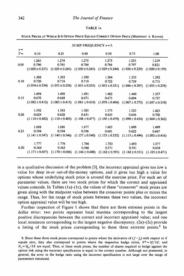
in a qualitative discussion of the problem [3], the incorrect appraisal gives too low a value for deep in-or out-of-the-money options, and it gives too high a value for options whose underlying stock price is around the exercise price. For each set of parameter values, there are two stock prices for which the correct and appraised values coincide. In Tables (la)-(lc), the values of these "crossover" stock prices are given along with the midpoint value between the crossover points plus or minus the range. Thus, for the range of stock prices between these two values, the incorrect option appraisal value will be too high.

Further inspection of Figure 1 shows that there are three extreme points in the dollar error: two points represent local maxima corresponding to the largest positive discrepancies between the correct and incorrect appraised value; and one local minimum corresponding to the largest negative discrepancy. (2a)-(2c) provide a listing of the stock prices corresponding to these three extreme points.8 In

8. Since these three stock prices correspond to points where the derivative of (f-fe) with respect to X equals zero, they also correspond to points where the respective hedge ratios, N* = af/ ax, and Ne = afe/ aX are equal. Thus, at these stock prices, the number of shares required to hedge against the option risk using the incorrect specification is equal to the correct number. Although not presented, in general, the error in the hedge ratio using the incorrect specification is not large over the range of parameters simulated.

The Impact on Option Pricing of Specification Error 343

TABLE lb

STOCK PRIUCES AT WHICH B-S OPTION PRICE EQUALS CORRECT OPTION PRICE (MIDPOINT ? RANGE)

JUMP FREQUENCYv = 10.

T= 0.10 0.25 0.40 0.50 0.75 1.00

1.259 1.262 1.260 1.256 1.237 1.196 0.05 0.794 0.792 0.793 0.796 0.809 0.836

(1.027 ? 0.233) (1.027 ?0.235) (1.027? 0.234) (1.026+0.230) (1.023 ? 0.214) (1.016 ? 0.180)

1.387 1.385 1.379 1.374 1.342 1.280 0.10 0.723 0.722 0.725 0.728 0.745 0.781

(1.055?0.332) (1.054?0.331) (1.052?0.327) (1.051 ?0.323) (1.044?0.299) (1.031 ?0.249)

1.492 1.490 1.484 1.477 1.441 1.371 0.15 0.672 0.672 0.674 0.677 0.694 .730

(1.082?0.410) (1.081 ?0.409) (1.079?0.405) (1.077?0.400) (1.068?0.373) (1.050?0.320)

1.590 1.587 1.581 1.573 1.536 1.466 0.20 0.631 0.630 0.633 0.636 0.651 0.682

(1.110?0.480) (1.109?0.478) (1.107?0.474) (1.104?0.468) (1.093?0.442) (1.074?0.392)

1.684 1.680 1.674 1.666 1.627 1.561 0.25 0.595 0.595 0.598 0.601 0.615 0.640

(1.139?0.544) (1.138?0.542) (1.136?0.538) (1.133?0.532) (1.121?0.506) (1.101 ?0.460)

1.773 1.770 1.764 1.755 1;717 1.653 0.30 0.566 0.565 0.567 0.570 0.582 0.605

(1.170?0.604) (1.167?0.602) (1.165?0.598) (1.162?0.592) (1.150?0.568) (1.129?0.524)

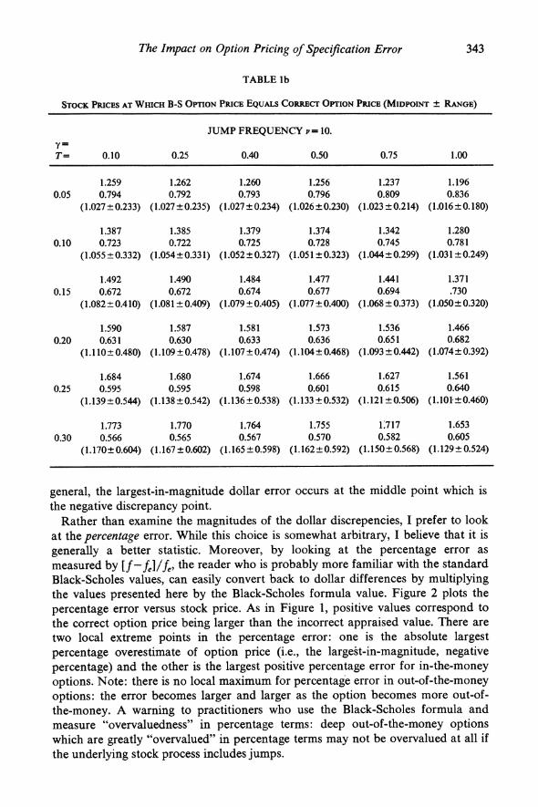
general, the largest-in-magnitude dollar error occurs at the middle point which is the negative discrepancy point.

Rather than examine the magnitudes of the dollar discrepencies, I prefer to look at the percentage error. While this choice is somewhat arbitrary, I believe that it is generally a better statistic. Moreover, by looking at the percentage error as measured by [f-fe]/fe the reader who is probably more familiar with the standard Black-Scholes values, can easily convert back to dollar differences by multiplying the values presented here by the Black-Scholes formula value. Figure 2 plots the percentage error versus stock price. As in Figure 1, positive values correspond to the correct option price being larger than the incorrect appraised value. There are two local extreme points in the percentage error: one is the absolute largest percentage overestimate of option price (i.e., the largest-in-magnitude, negative percentage) and the other is the largest positive percentage error for in-the-money options. Note: there is no local maximum for percentage error in out-of-the-money options: the error becomes larger and larger as the option becomes more out-of- the-money. A warning to practitioners who use the Black-Scholes formula and measure "overvaluedness" in percentage terms: deep out-of-the-money options which are greatly "overvalued" in percentage terms may not be overvalued at all if the underlying stock process includes jumps.

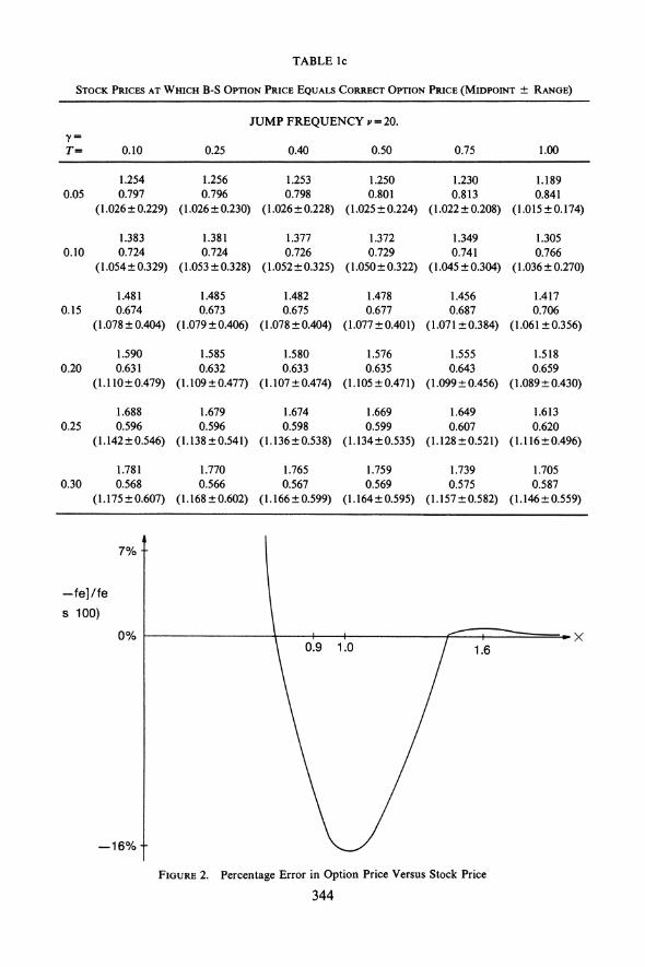
TABLE Ic

STOCK PRICES AT WHICH B-S OPTION PRICE EQUALS CORRECT OPTION PRICE (MIDPOINT ? RANGE)

JUMP FREQUENCY v=20.

T= 0.10 0.25 0.40 0.50 0.75 1.00

1.254 1.256 1.253 1.250 1.230 1.189 0.05 0.797 0.796 0.798 0.801 0.813 0.841

(1.026? 0.229) (1.026 ? 0.230) (1.026 ? 0.228) (1.025 ? 0.224) (1.022 ? 0.208) (1.015 ? 0.174)

1.383 1.381 1.377 1.372 1.349 1.305 0.10 0.724 0.724 0.726 0.729 0.741 0.766

(1.054?0.329) (1.053 ? 0.328) (1.052?0.325) (1.050?0.322) (1.045 ?0.304) (1.036? 0.270)

1.481 1.485 1.482 1.478 1.456 1.417 0.15 0.674 0.673 0.675 0.677 0.687 0.706

(1.078?0.404) (1.079?0.406) (1.078?0.404) (1.077?0.401) (1.071 ?0.384) (1.061 ?0.356)

1.590 1.585 1.580 1.576 1.555 1.518 0.20 0.631 0.632 0.633 0.635 0.643 0.659

(1.110?0.479) (1.109?0.477) (1.107?0.474) (1.105?0.471) (1.099?0.456) (1.089?0.430)

1.688 1.679 1.674 1.669 1.649 1.613 0.25 0.596 0.596 0.598 0.599 0.607 0.620

(1.142?0.546) (1.138?0.541) (1.136?0.538) (1.134?0.535) (1.128?0.521) (1.116?0.496)

1.781 1.770 1.765 1.759 1.739 1.705 0.30 0.568 0.566 0.567 0.569 0.575 0.587

(1.175?0.607) (1.168?0.602) (1.166?0.599) (1.164?0.595) (1.157?0.582) (1.146?0.559)

7%

-fe]/fe s 1 00)

0% X 0.9 1.0 1.6

-16%

FIGURE 2. Percentage Error in Option Price Versus Stock Price

344

The Impact on Option Pricing of Specification Error 345

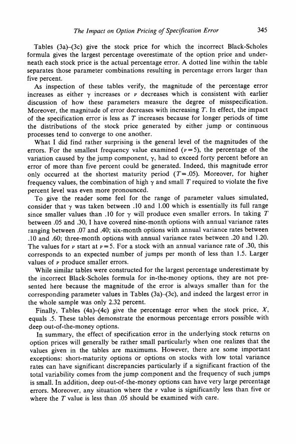
Tables (3a)-(3c) give the stock price for which the incorrect Black-Scholes formula gives the largest percentage overestimate of the option price and under- neath each stock price is the actual percentage error. A dotted line within the table separates those parameter combinations resulting in percentage errors larger than five percent.

As inspection of these tables verify, the magnitude of the percentage error increases as either y increases or v decreases which is consistent with earlier discussion of how these parameters measure the degree of misspecification. Moreover, the magnitude of error decreases with increasing T. In effect, the impact of the specification error is less as T increases because for longer periods of time the distributions of the stock price generated by either jump or continuous processes tend to converge to one another.

What I did find rather surprising is the general level of the magnitudes of the errors. For the smallest frequency value examined (v = 5), the percentage of the variation caused by the jump component, y, had to exceed forty percent before an error of more than five percent could be generated. Indeed, this magnitude error only occurred at the shortest maturity period (T= .05). Moreover, for higher frequency values, the combination of high y and small T required to violate the five percent level was even more pronounced.

To give the reader some feel for the range of parameter values simulated, consider that y was taken between .10 and 1.00 which is essentially its full range since smaller values than .10 for y will produce even smaller errors. In taking T between .05 and .30, I have covered nine-month options with annual variance rates ranging between .07 and .40; six-month options with annual variance rates between .10 and .60; three-month options with annual variance rates between .20 and 1.20. The values for v start at v= 5. For a stock with an annual variance rate of .30, this corresponds to an expected number of jumps per month of less than 1.5. Larger values of v produce smaller errors.

While similar tables were constructed for the largest percentage underestimate by the incorrect Black-Scholes formula for in-the-money options, they are not pre- sented here because the magnitude of the error is always smaller than for the corresponding parameter values in Tables (3a)-(3c), and indeed the largest error in the whole sample was only 2.32 percent.

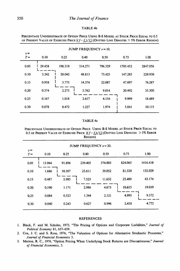
Finally, Tables (4a)-(4c) give the percentage error when the stock price, X, equals .5. These tables demonstrate the enormous percentage errors possible with deep out-of-the-money options.

In summary, the effect of specification error in the underlying stock returns on option prices will generally be rather small particularly when one realizes that the values given in the tables are maximums. However, there are some important exceptions: short-maturity options or options on stocks with low total variance rates can have significant discrepancies particularly if a significant fraction of the total variability comes from the jump component and the frequency of such jumps is small. In addition, deep out-of-the-money options can have very large percentage errors. Moreover, any situation where the v value is significantly less than five or where the T value is less than .05 should be examined with care.

TABLE 2a

TABLE 2b

STOCK

PRICES

AT

WHICH

THERE IS A

LOCAL

MAXIMUM

OF

THE

DOLLAR

ERROR

IN

STOCK

PRICES

AT

WHICH

THERE IS A

LOCAL

MAXIMUM

OF

THE

DOLLAR

ERROR

IN

OPTION

PRICE

OPTION

PRICE

JUMP

FREQUENCY v = 5.

JUMP

FREQUENCY v = 10.

T=

0.10

0.25

0.40

0.50

0.75

1.00

T=

0.10

0.25

0.40

0.50

0.75

1.00

0.672

0.666

0.665

0.667

0.680

0.695

0.678

0.675

0.678

0.681

0.697

0.717

0.05

1.009

1.009

1.009

1.009

1.007

1.000

0.05

1.009

1.009

1.008

1.008

1.006

1.000

1.513

1.532

1.535

1.531

1.506

1.480

1.495

1.507

1.503

1.495

1.463

1.425

0.579

0.576

0.579

0.583

0.602

0.628

0.583

0.582

0.585

0.590

0.610

0.636

0.10

1.018

1.018

1.017

1.017

1.013

1.000

0.10

1.018

1.018

1.017

1.016

1.013

1.000

1.778

1.798

1.791

1.779

1.724

1.666

1.762

1.778

1.768

1.755

1.700

1.640

0.516

0.514

0.518

0.523

0.546

0.577

0.519

0.518

0.522

0.526

0.544

0.566

0.15

1.027

1.027

1.026

1.024

1.019

1.000

0.15

1.028

1.027

1.025

1.024

1.019

1.000

2.017

2.045

2.033

2.014

1.934

1.848

1.953

2.017

2.013

1.999

1.938

1.877

0.468

0.467

0.471

0.476

0.499

0.530

0.470

0.470

0.473

0.477

0.492

0.511

0.20

1.038

1.036

1.035

1.033

1.026

1.000

0.20

1.039

1.036

1.034

1.033

1.027

1.000

2.254

2.287

2.272

2.249

2.152

2.049

2.078

2.236

2.245

2.234

2.173

2.112

0.430

0.429

0.433

0.438

0.459

0.488

0.431

0.431

0.434

0.437

0.451

0.467

0.25

1.048

1.045

1.043

1.042

1.033

1.000

0.25

1.053

1.045

1.044

1.043

1.036

1.000

2.341

2.499

2.500

2.479

2.375

2.271

2.181

2.438

2.472

2.465

2.407

2.340

0.398

0.397

0.401

0.405

0.425

0.451

0.399

0.399

0.401

0.404

0.416

0.432

0.30

1.057

1.054

1.052

1.050

1.041

1.000

0.30

1.057

1.055

1.053

1.051

1.045

1.000

2.605

2.752

2.748

2.722

2.610

2.507

2.424

2.622

2.690

2.694

2.643

2.569

346

TABLE 2c

STOCK

PRICES

AT

WHICH

THERE IS A

LOCAL

MAXIMUM

OF

THE

DOLLAR

ERROR

IN

OPTION

PRICE

JUMP

FREQUENCY v = 20.

T=

0.10

0.25

0.40

0.50

0.75

1.00

0.681

0.680

0.683

0.687

0.703

0.724

0.05

1.009

1.009

1.009

1.008

1.006

1.000

1.487

1.495

1.489

1.481

1.448

1.411

0.584

0.584

0.587

0.590

0.603

0.619

0.10

1.018

1.017

1.017

1.016

1L013

1.000

1.748

1.767

1.761

1.753

1.716

1.679

0.519

0.520

0.522

0.525

0.535

0.549

0.15

1.028

1.026

1.025

1.025

1.022

1.000

1.925

2.005

2.007

2.000

1.964

1.920

0.471

0.471

0.473

0.475

0.484

0.497

0.20

1.041

1.036

1.035

1.034

1.030

1.000

2.089

2.232

2.246

2.240

2.205

2.157

0.432

0.432

0.434

0.435

0.443

0.455

0.25

1.052

1.045

1.044

1.043

1.040

1.000

2.238

2.347

2.433

2.446

2.430

2.384

0.399

0.400

0.401

0.403

0.409

0.419

0.30

1.070

1.057

1.054

1.053

1.049

1.025

2.131

2.549

2.656

2.679

2.669

2.623

347

TABLE 3a

MAXIMUM PERCENTAGE OVERESTIMAGE OF OPTION PRICE USING B-S MODEL: STOCK PRICE

AND PERCENTAGE ERROR [(frfe)/fe] (DOTTED LINE DENOTES > 5% ERROR REGION)

JUMP FREQUENCY v= 5.

lY= T= 0.10 0.25 0.40 0.50 0.75 1.00

0.05 0.898 0.894 j 0.894 0.897 0.915 1.000 -0.6026 -3.3410 1 -7.8810 -11.8250 -25.1344 -53.7471

L -_-

0.10 0.862 0.861 0.864 0.869 0.893 1.000 - 0.3238 - 1.8998 - 4.6791 -7.2037 - 16.3082 - 38.7856

0.15 0.835 0.835 0.839 0.845 0.874 1.000 -0.2228 - 1.3362 - 3.3427 1 -5.1923 -11.9991 -29.4940

0.20 0.813 0.812 0.817 0.823 0.856 1.000 -0.1711 - 1.0361 -2.6105 -4.0689 / -9.4506 -23.1573

0.25 0.792 0.791 0.797 0.804 j 0.838 1.000 -0.1395 -0.8495 -2.1486 -3.3535 j -7.7826 - 18.6090

0.30 0.773 0.773 0.778 0.785 0.819 1.000 -0.1180 -0.7222 - 1.8309 -2.8596 -6.6162 - 15.2494

TABLE 3b

MAXIMUM PERCENTAGE OVERESTIMATE OF OPTION PRICE USING B-S MODEL: STOCK PRICE

AND PERCENTAGE ERROR [(f-fe)/fe] (DOTTED LINE DENOTES > 5% ERROR REGION)

JUMP FREQUENCY v= 10.

T= 0.10 0.25 0.40 0.50 0.75 1.00

0.05 0.902 0.900 0.903 I 0.907 0.924 1.000 -0.3196 - 1.8750 -4.6185 I -7.1127 - 16.1295 -38.4699

0.10 0.866 0.866 0.869 0.874 1 0.897 1.000 -0.1670 -1.0109 -2.5482 -3.9746 1 -9.2613 -22.9271

0.15 0.838 0.837 0.842 0.847 I 0.872 1.000 -0.1139 -0.6969 - 1.7679 -2.7638 1 -6.4212 - 15.0055

L -

0.20 0.815 0.814 0.818 0.823 0.848 1 1.000 -0.0870 -0.5347 - 1.3599 -2.1268 - 4.9096 1 -10.5151

0.25 0.796 0.794 0.797 0.802 0.825 1.000 -0.0709 -0.4357 - 1.1097 - 1.7352 -3.9837 -7.7948

0.30 0.775 0.774 0.778 0.782 0.804 0.919 - 0.0595 -0.3684 -0.9395 -1.4691 - 3.3609 -6.1770

348

TABLE 3c

MAXIMUM PERCENTAGE OVERESTIMATE OF OPTION PRICE USING B-S MODEL: STOCK PRICE

AND PERCENTAGE ERROR [(f-fe)/fe] (DOTTED LINE DENOTES > 5% ERROR REGION)

JUMP FREQUENCY v = 20.

Y= T= 0.10 0.25 0.40 0.50 0.75 1.00

0.05 0.903 0.904 0.907 0.911 1 0.927 1.000 -0.1649 -0.9984 -2.5171 - 3.9274 - 9.1656 -22.7835

0.10 0.867 0.867 0.870 0.874 0.892 1.000 -0.0849 -0.5219 - 1.3280 -2.0778 -4.8089 - 10.3987

0.15 0.840 0.839 0.841 0.845 0.861 0.948 -0.0576 -0.3557 -0.9075 - 1.4199 -3.2564 -6.0423

0.20 0.818 0.815 0.817 0.820 0.834 0.879 - 0.0438 -0.2715 - 0.6932 - 1.0842 - 2.4736 -4.4655

0.25 0.797 0.794 0.796 0.799 0.811 0.842 - 0.0356 -0.2205 -0.5632 -0.8808 -2.0029 -3.6129

0.30 0.780 0.776 0.777 0.779 0.790 0.815 - 0.0298 -0.1860 - 0.4756 -0.7436 - 1.6879 - 3.0454

TABLE 4a

PERCENTAGE UNDERESTIMATE OF OPTION PRICE USING B-S MODEL AT STOCK PRICE EQUAL TO 0.5 OF

PRESENT VALUE OF EXERCISE PRICE [(f-fe)/fe] (DOTTED LINE DENOTES > 5% ERROR REGION)

JUMP FREQUENCY v= 5.

Y= T= 0.10 0.25 0.40 0.50 0.75 1.00

0.05 j 64.181 437.295 1114.618 1701.564 3515.315 5670.387

0.10 1 6.557 38.036 90.143 133.628 260.985 400.115

0.15 1.865 1 10.858 26.417 40.141 83.696 132.234

0.20 0.727 4.285 1 10.710 16.686 37.754 63.376

0.25 0.323 1.925 4.922 7.846 19.296 35.048

0.30 0.148 0.887 2.323 3.797 10.267 20.585

349

350 The Journal of Finance

TABLE 4b

PERCENTAGE UNDERESTIMATE OF OPTION PRICE USING B-S MODEL AT STOCK PRICE EQUAL TO 0.5 OF PRESENT VALUE OF EXERCISE PRICE [(f-fe)/fel (DOTTED LINE DENOTES > 5% ERROR REGION)

JUMP FREQUENCY v= 10.

T= 0.10 0.25 0.40 0.50 0.75 1.00

0.05 1 29.458 198.319 514.271 796.329 1705.452 2847.056 L - -

0.10 3.342 1 20.042 48.813 73.425 147.285 229.930

0.15 0.958 t 5.775 14.374 22.087 47.097 76.287 L -

0.20 0.374 2.273 I 5.762 9.014 20.492 35.300

0.25 0.167 1.018 2.617 4.154 I 9.999 18.489

0.30 0.078 0.472 1.227 1.974 5.041 10.115

TABLE 4c

PERCENTAGE UNDERESTIMATE OF OPTION PRICE USING B-S MODEL AT STOCK PRICE EQUAL TO

0.5 OF PRESENT VALUE OF EXERCISE PRICE [(ffe)/fel (DOTTED LINE DENOTES > 5% ERROR

REGION)

JUMP FREQUENCY I=20.

T= 0.10 0.25 0.40 0.50 0.75 1.00

0.05 I 13.964 91.896 239.405 374.003 824.065 1416.418

0.10 1.686 1 10.307 25.611 39.052 81.320 132.029 L - - --

0.15 0.487 2.985 1 7.525 11.652 25.489 43.174 L- - - - m _-

0.20 0.190 1.171 2.986 4.673 1 10.655 19.019

0.25 0.084 0.523 1.344 2.121 4.995 1 9.372

0.30 0.040 0.243 0.627 0.996 2.418 4.775

REFERENCES

1. Black, F. and M. Scholes, 1973, "The Pricing of Options and Corporate Liabilities," Journal of Political Economy 81, 637-659.

2. Cox, J. C. and S. Ross, 1976, "The Valuation of Options for Alternative Stochastic Processes," Journal of Financial Economics 3.

3. Merton, R. C., 1976, "Option Pricing When Underlying Stock Returns are Discontinuous," Journal of Financial Economics, 3.