amortized analysis binomial heaps fibonacci heaps … · 9 amortized analysis worst-case analysis....
TRANSCRIPT
Lecture slides by Kevin Waynehttp://www.cs.princeton.edu/~wayne/kleinberg-tardos
Last updated on Apr 8, 2013 6:13 AM
DATA STRUCTURES
‣ amortized analysis
‣ binomial heaps
‣ Fibonacci heaps
‣ union-find
2
Data structures
Static problems. Given an input, produce an output.
Ex. Sorting, FFT, edit distance, shortest paths, MST, max-flow, ...
Dynamic problems. Given a sequence of operations (given one at a time),
produce a sequence of outputs.
Ex. Stack, queue, priority queue, symbol table, union-find, ….
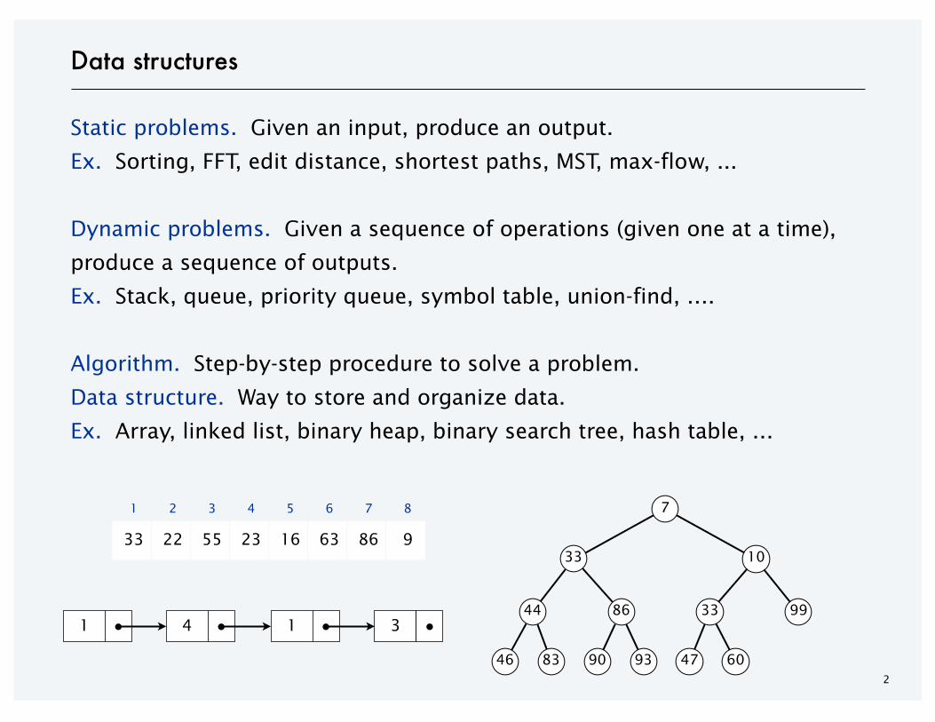
Algorithm. Step-by-step procedure to solve a problem.
Data structure. Way to store and organize data.
Ex. Array, linked list, binary heap, binary search tree, hash table, …
7
33
44
46 83
86
90 93
10
33
47 60
99
1 2 3 4 5 6 7 8
33 22 55 23 16 63 86 9
1 ● 4 ● 1 ● 3 ●
3
Appetizer
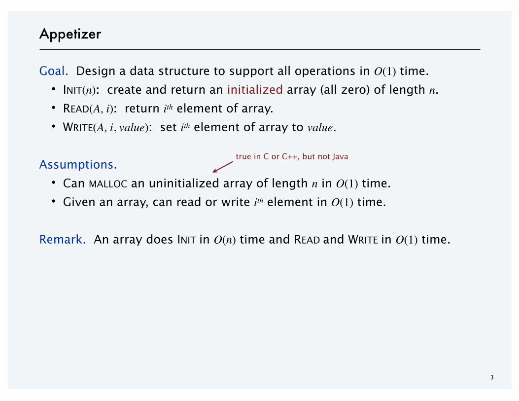
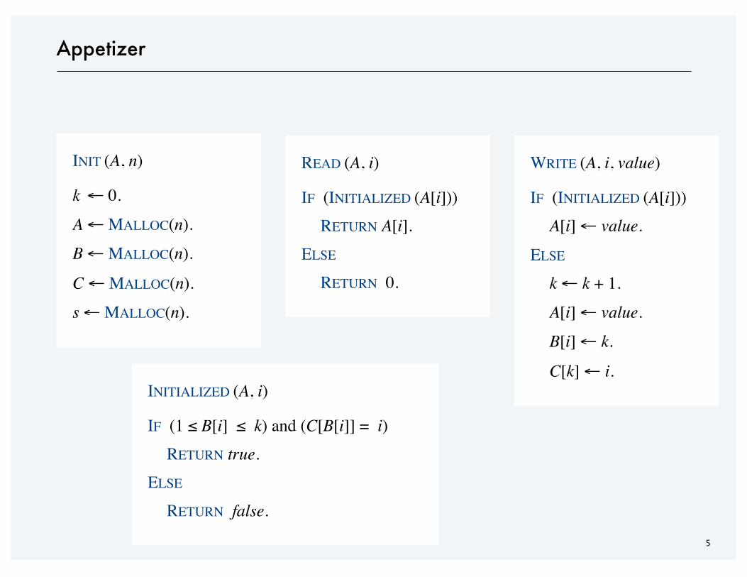
Goal. Design a data structure to support all operations in O(1) time.
・INIT(n): create and return an initialized array (all zero) of length n.
・READ(A, i): return ith element of array.
・WRITE(A, i, value): set ith element of array to value.
Assumptions.
・Can MALLOC an uninitialized array of length n in O(1) time.
・Given an array, can read or write ith element in O(1) time.
Remark. An array does INIT in O(n) time and READ and WRITE in O(1) time.
true in C or C++, but not Java
4
Appetizer
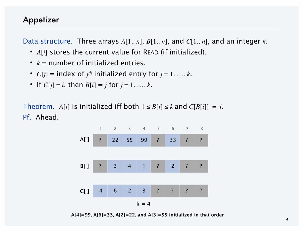
Data structure. Three arrays A[1.. n], B[1.. n], and C[1.. n], and an integer k.
・A[i] stores the current value for READ (if initialized).
・k = number of initialized entries.
・C[j] = index of jth initialized entry for j = 1, …, k.
・If C[j] = i, then B[i] = j for j = 1, …, k.
Theorem. A[i] is initialized iff both 1 ≤ B[i] ≤ k and C[B[i]] = i.Pf. Ahead.
1 2 3 4 5 6 7 8
? 22 55 99 ? 33 ? ?A[ ]
? 3 4 1 ? 2 ? ?B[ ]
A[4]=99, A[6]=33, A[2]=22, and A[3]=55 initialized in that order
k = 4
4 6 2 3 ? ? ? ?C[ ]
5
Appetizer
READ (A, i) ___________________________________________________________________________________________________________________________________________________________________________________________________________________________________________________________________________________________________________________________________________________________________________________________________________________________________________________________________________________
IF (INITIALIZED (A[i]))RETURN A[i].
ELSE
RETURN 0. ___________________________________________________________________________________________________________________________________________________________________________________________________________________________________________________________________________________________________________________________________________________________________________________________________________________________________________________________________________________
WRITE (A, i, value) ___________________________________________________________________________________________________________________________________________________________________________________________________________________________________________________________________________________________________________________________________________________________________________________________________________________________________________________________________________________
IF (INITIALIZED (A[i]))A[i] ← value.
ELSE
k ← k + 1.
A[i] ← value.
B[i] ← k.
C[k] ← i. ___________________________________________________________________________________________________________________________________________________________________________________________________________________________________________________________________________________________________________________________________________________________________________________________________________________________________________________________________________________INITIALIZED (A, i)
_______________________________________________________________________________________________________________________________________________________________________________________________________________________________________________________________________________________________________________________________________________________________________________________________________________________________________________________________________________________________________________________________________________________________________________________________________________________________________________________________________________________________________________________________________________________________________
IF (1 ≤ B[i] ≤ k) and (C[B[i]] = i)RETURN true.
ELSE
RETURN false. _______________________________________________________________________________________________________________________________________________________________________________________________________________________________________________________________________________________________________________________________________________________________________________________________________________________________________________________________________________________________________________________________________________________________________________________________________________________________________________________________________________________________________________________________________________________________________
INIT (A, n) ___________________________________________________________________________________________________________________________________________________________________________________________________________________________________________________________________________________________________________________________________________________________________________________________________________________________________________________________________________________
k ← 0.
A ← MALLOC(n).
B ← MALLOC(n).
C ← MALLOC(n).
s ← MALLOC(n). ___________________________________________________________________________________________________________________________________________________________________________________________________________________________________________________________________________________________________________________________________________________________________________________________________________________________________________________________________________________
6
Appetizer
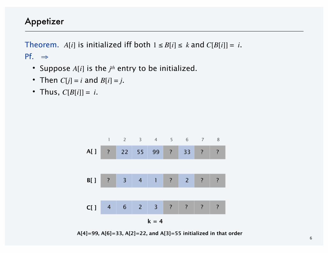
Theorem. A[i] is initialized iff both 1 ≤ B[i] ≤ k and C[B[i]] = i.Pf. ⇒
・Suppose A[i] is the jth entry to be initialized.
・Then C[j] = i and B[i] = j.
・Thus, C[B[i]] = i.
1 2 3 4 5 6 7 8
? 22 55 99 ? 33 ? ?A[ ]
? 3 4 1 ? 2 ? ?B[ ]
A[4]=99, A[6]=33, A[2]=22, and A[3]=55 initialized in that order
k = 4
4 6 2 3 ? ? ? ?C[ ]
7
Appetizer
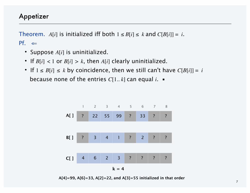
Theorem. A[i] is initialized iff both 1 ≤ B[i] ≤ k and C[B[i]] = i.Pf. ⇐
・Suppose A[i] is uninitialized.
・If B[i] < 1 or B[i] > k, then A[i] clearly uninitialized.
・If 1 ≤ B[i] ≤ k by coincidence, then we still can't have C[B[i]] = ibecause none of the entries C[1.. k] can equal i. ▪
1 2 3 4 5 6 7 8
? 22 55 99 ? 33 ? ?A[ ]
? 3 4 1 ? 2 ? ?B[ ]
A[4]=99, A[6]=33, A[2]=22, and A[3]=55 initialized in that order
k = 4
4 6 2 3 ? ? ? ?C[ ]

Lecture slides by Kevin Waynehttp://www.cs.princeton.edu/~wayne/kleinberg-tardos
Last updated on Apr 8, 2013 6:13 AM
AMORTIZED ANALYSIS
‣ binary counter
‣ multipop stack
‣ dynamic table
9
Amortized analysis
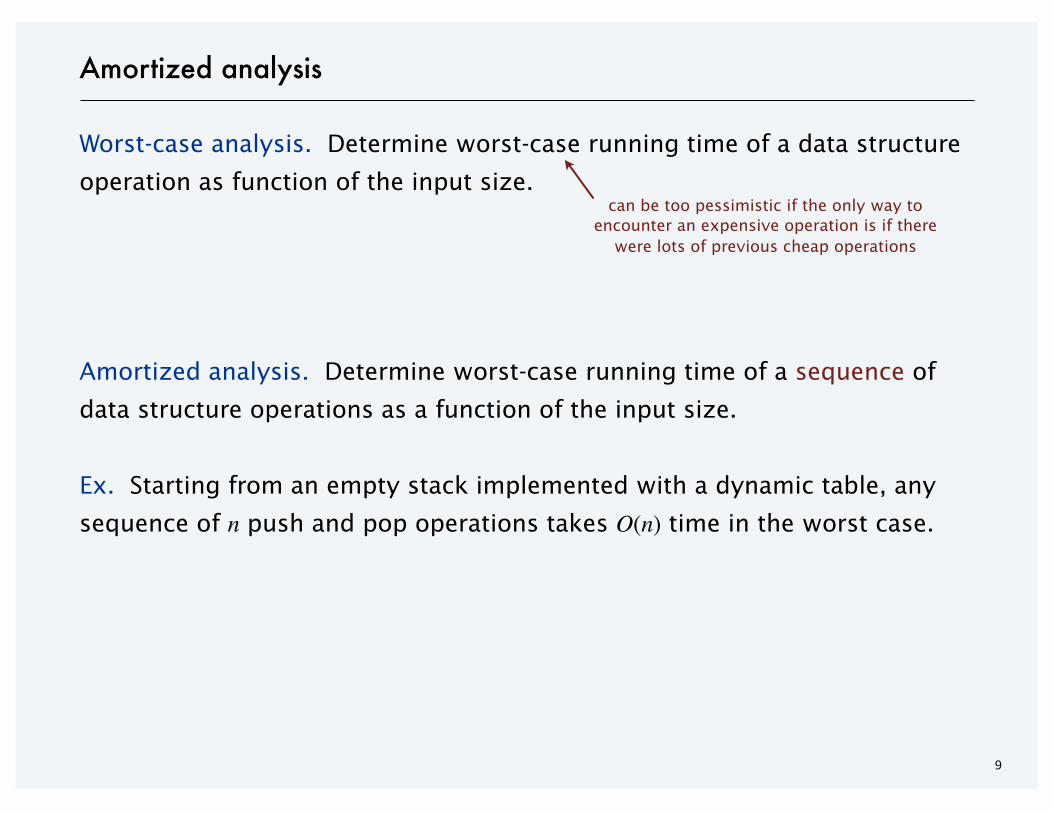
Worst-case analysis. Determine worst-case running time of a data structure
operation as function of the input size.
Amortized analysis. Determine worst-case running time of a sequence of
data structure operations as a function of the input size.
Ex. Starting from an empty stack implemented with a dynamic table, any
sequence of n push and pop operations takes O(n) time in the worst case.
can be too pessimistic if the only way toencounter an expensive operation is if there
were lots of previous cheap operations
10
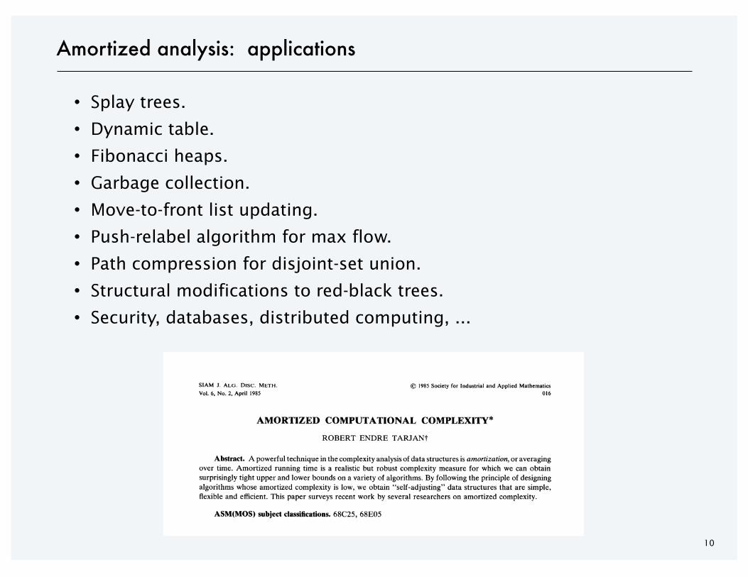
Amortized analysis: applications
・Splay trees.
・Dynamic table.
・Fibonacci heaps.
・Garbage collection.
・Move-to-front list updating.
・Push-relabel algorithm for max flow.
・Path compression for disjoint-set union.
・Structural modifications to red-black trees.
・Security, databases, distributed computing, ...
SIAM J. ALG. DISC. METH.Vol. 6, No. 2, April 1985
1985 Society for Industrial and Applied Mathematics016
AMORTIZED COMPUTATIONAL COMPLEXITY*ROBERT ENDRE TARJANt
Abstract. A powerful technique in the complexity analysis of data structures is amortization, or averagingover time. Amortized running time is a realistic but robust complexity measure for which we can obtainsurprisingly tight upper and lower bounds on a variety of algorithms. By following the principle of designingalgorithms whose amortized complexity is low, we obtain "self-adjusting" data structures that are simple,flexible and efficient. This paper surveys recent work by several researchers on amortized complexity.
ASM(MOS) subject classifications. 68C25, 68E05
1. Introduction. Webster’s [34] defines "amortize" as "to put money aside atintervals, as in a sinking fund, for gradual payment of (a debt, etc.)." We shall adaptthis term to computational complexity, meaning by it "to average over time" or, moreprecisely, "to average the running times of operations in a sequence over the sequence."The following observation motivates our study of amortization: In many uses of datastructures, a sequence of operations, rather than just a single operation, is performed,and we are interested in the total time of the sequence, rather than in the times ofthe individual operations. A worst-case analysis, in which we sum the worst-case timesof the individual operations, may be unduly pessimistic, because it ignores correlatedeffects of the operations on the data structure. On the other hand, an average-caseanalysis may be inaccurate, since the probabilistic assumptions needed to carry outthe analysis may be false. In such a situation, an amortized analysis, in which weaverage the running time per operation over a (worst-case) sequence of operations,can yield an answer that is both realistic and robust.
To make the idea of amortization and the motivation behind it more concrete,let us consider a very simple example. Consider the manipulation of a stack by asequence of operations composed of two kinds of unit-time primitives: push, whichadds a new item to the top of the stack, and pop, which removes and returns the topitem on the stack. We wish to analyze the running time of a sequence of operations,each composed of zero or more pops followed by a push. Assume we start with anempty stack and carry out m such operations. A single operation in the sequence cantake up to m time units, as happens if each of the first m- 1 operations performs nopops and the last operation performs m 1 pops. However, altogether the m operationscan perform at most 2m pushes and pops, since there are only m pushes altogetherand each pop must correspond to an earlier push.
This example may seem too simple to be useful, but such stack manipulationindeed occurs in applications as diverse as planarity-testing [14] and related problems[24] and linear-time string matching [18]. In this paper we shall survey a number ofsettings in which amortization is useful. Not only does amortized running time providea more exact way to measure the running time of known algorithms, but it suggeststhat there may be new algorithms efficient in an amortized rather than a worst-casesense. As we shall see, such algorithms do exist, and they are simpler, more efficient,and more flexible than their worst-case cousins.
* Received by the editors December 29, 1983. This work was presented at the SIAM Second Conferenceon the Applications of Discrete Mathematics held at Massachusetts Institute of Technology, Cambridge,Massachusetts, June 27-29, 1983.
t Bell Laboratories, Murray Hill, New Jersey 07974.
306
CHAPTER 17
AMORTIZED ANALYSIS
‣ binary counter
‣ multipop stack
‣ dynamic table
12
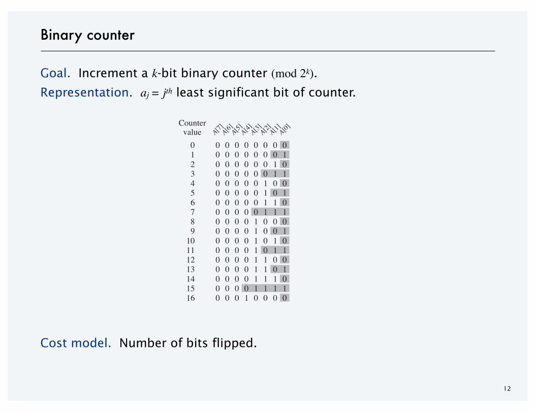
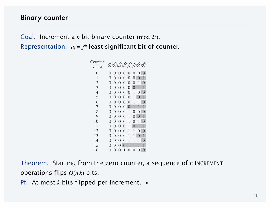
Binary counter
Goal. Increment a k-bit binary counter (mod 2k).Representation. aj = jth least significant bit of counter.
Cost model. Number of bits flipped.
17.1 Aggregate analysis 455
0 0 0 0 0 0 0 000 0 0 0 0 0 0 110 0 0 0 0 0 1 020 0 0 0 0 0 1 130 0 0 0 0 1 0 040 0 0 0 0 1 0 150 0 0 0 0 1 1 060 0 0 0 0 1 1 170 0 0 0 1 0 0 080 0 0 0 1 0 0 190 0 0 0 1 0 1 0100 0 0 0 1 0 1 1110 0 0 0 1 1 0 0120 0 0 0 1 1 0 1130 0 0 0 1 1 1 0140 0 0 0 1 1 1 1150 0 0 1 0 0 0 016
A[0]A[1]A[2]A[3]A[4]A[5]A[6]A[7]Counter
valueTotalcost
13478
1011151618192223252631
0
Figure 17.2 An 8-bit binary counter as its value goes from 0 to 16 by a sequence of 16 INCREMENToperations. Bits that flip to achieve the next value are shaded. The running cost for flipping bits isshown at the right. Notice that the total cost is always less than twice the total number of INCREMENToperations.
operations on an initially zero counter causes AŒ1! to flip bn=2c times. Similarly,bit AŒ2! flips only every fourth time, or bn=4c times in a sequence of n INCREMENToperations. In general, for i D 0; 1; : : : ; k ! 1, bit AŒi ! flips bn=2ic times in asequence of n INCREMENT operations on an initially zero counter. For i " k,bit AŒi ! does not exist, and so it cannot flip. The total number of flips in thesequence is thusk!1X
iD0
j n
2i
k< n
1X
iD0
1
2i
D 2n ;
by equation (A.6). The worst-case time for a sequence of n INCREMENT operationson an initially zero counter is therefore O.n/. The average cost of each operation,and therefore the amortized cost per operation, is O.n/=n D O.1/.
13
Binary counter
Goal. Increment a k-bit binary counter (mod 2k).Representation. aj = jth least significant bit of counter.
Theorem. Starting from the zero counter, a sequence of n INCREMENT
operations flips O(n k) bits.
Pf. At most k bits flipped per increment. ▪
17.1 Aggregate analysis 455
0 0 0 0 0 0 0 000 0 0 0 0 0 0 110 0 0 0 0 0 1 020 0 0 0 0 0 1 130 0 0 0 0 1 0 040 0 0 0 0 1 0 150 0 0 0 0 1 1 060 0 0 0 0 1 1 170 0 0 0 1 0 0 080 0 0 0 1 0 0 190 0 0 0 1 0 1 0100 0 0 0 1 0 1 1110 0 0 0 1 1 0 0120 0 0 0 1 1 0 1130 0 0 0 1 1 1 0140 0 0 0 1 1 1 1150 0 0 1 0 0 0 016
A[0]A[1]A[2]A[3]A[4]A[5]A[6]A[7]Counter
valueTotalcost
13478
1011151618192223252631
0
Figure 17.2 An 8-bit binary counter as its value goes from 0 to 16 by a sequence of 16 INCREMENToperations. Bits that flip to achieve the next value are shaded. The running cost for flipping bits isshown at the right. Notice that the total cost is always less than twice the total number of INCREMENToperations.
operations on an initially zero counter causes AŒ1! to flip bn=2c times. Similarly,bit AŒ2! flips only every fourth time, or bn=4c times in a sequence of n INCREMENToperations. In general, for i D 0; 1; : : : ; k ! 1, bit AŒi ! flips bn=2ic times in asequence of n INCREMENT operations on an initially zero counter. For i " k,bit AŒi ! does not exist, and so it cannot flip. The total number of flips in thesequence is thusk!1X
iD0
j n
2i
k< n
1X
iD0
1
2i
D 2n ;
by equation (A.6). The worst-case time for a sequence of n INCREMENT operationson an initially zero counter is therefore O.n/. The average cost of each operation,and therefore the amortized cost per operation, is O.n/=n D O.1/.
14
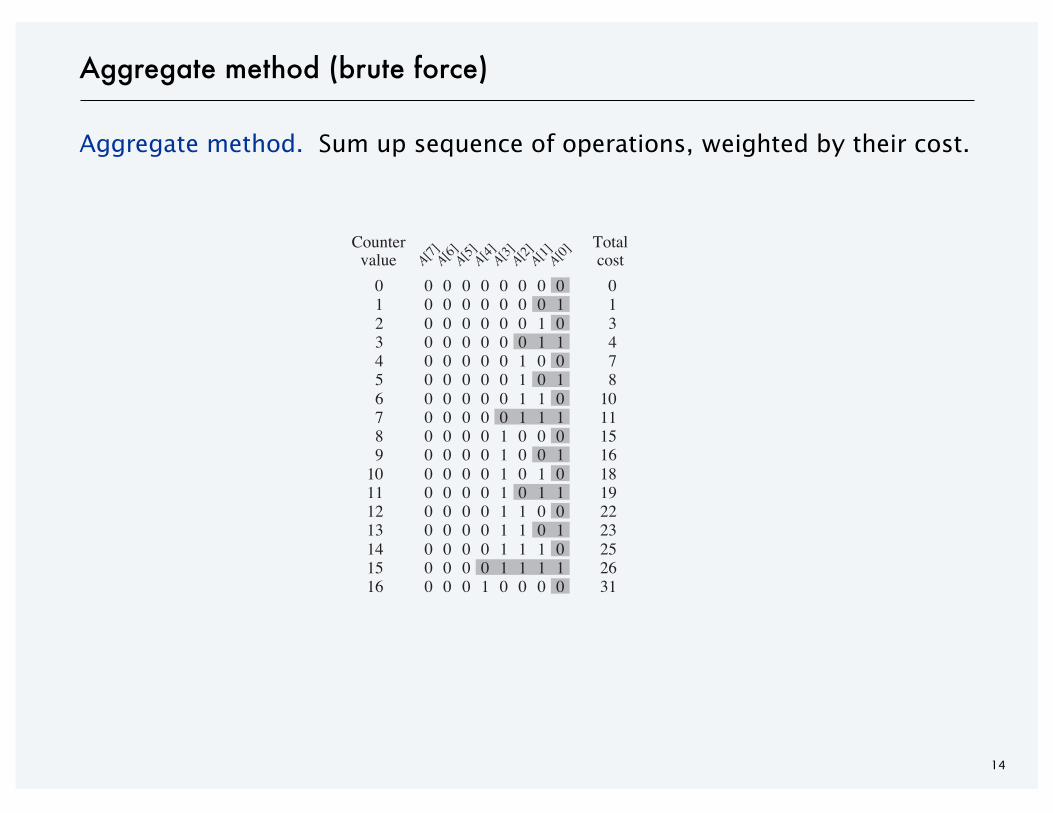
Aggregate method (brute force)
Aggregate method. Sum up sequence of operations, weighted by their cost.
17.1 Aggregate analysis 455
0 0 0 0 0 0 0 000 0 0 0 0 0 0 110 0 0 0 0 0 1 020 0 0 0 0 0 1 130 0 0 0 0 1 0 040 0 0 0 0 1 0 150 0 0 0 0 1 1 060 0 0 0 0 1 1 170 0 0 0 1 0 0 080 0 0 0 1 0 0 190 0 0 0 1 0 1 0100 0 0 0 1 0 1 1110 0 0 0 1 1 0 0120 0 0 0 1 1 0 1130 0 0 0 1 1 1 0140 0 0 0 1 1 1 1150 0 0 1 0 0 0 016
A[0]A[1]A[2]A[3]A[4]A[5]A[6]A[7]Counter
valueTotalcost
13478
1011151618192223252631
0
Figure 17.2 An 8-bit binary counter as its value goes from 0 to 16 by a sequence of 16 INCREMENToperations. Bits that flip to achieve the next value are shaded. The running cost for flipping bits isshown at the right. Notice that the total cost is always less than twice the total number of INCREMENToperations.
operations on an initially zero counter causes AŒ1! to flip bn=2c times. Similarly,bit AŒ2! flips only every fourth time, or bn=4c times in a sequence of n INCREMENToperations. In general, for i D 0; 1; : : : ; k ! 1, bit AŒi ! flips bn=2ic times in asequence of n INCREMENT operations on an initially zero counter. For i " k,bit AŒi ! does not exist, and so it cannot flip. The total number of flips in thesequence is thusk!1X
iD0
j n
2i
k< n
1X
iD0
1
2i
D 2n ;
by equation (A.6). The worst-case time for a sequence of n INCREMENT operationson an initially zero counter is therefore O.n/. The average cost of each operation,and therefore the amortized cost per operation, is O.n/=n D O.1/.

15
Binary counter: aggregate method
Starting from the zero counter, in a sequence of n INCREMENT operations:
・Bit 0 flips n times.
・Bit 1 flips ⎣ n / 2⎦ times.
・Bit 2 flips ⎣ n / 4⎦ times.
・…
Theorem. Starting from the zero counter, a sequence of n INCREMENT
operations flips O(n) bits.
Pf.
・Bit j flips ⎣ n / 2 j⎦ times.
・The total number of bits flipped is
Remark. Theorem may be false if initial counter is not zero.
k�1�
j=0
� n
2j
�< n
��
j=0
1
2j
= 2n ▪
k�1�
j=0
� n
2j
�< n
��
j=0
1
2j
= 2n
16
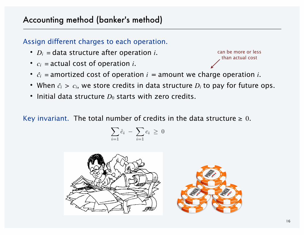
Accounting method (banker's method)
Assign different charges to each operation.
・Di = data structure after operation i.
・ci = actual cost of operation i.
・ĉi = amortized cost of operation i = amount we charge operation i.
・When ĉi > ci, we store credits in data structure Di to pay for future ops.
・Initial data structure D0 starts with zero credits.
Key invariant. The total number of credits in the data structure ≥ 0.n�
i=1
ci �n�
i=1
ci � 0
can be more or lessthan actual cost
17
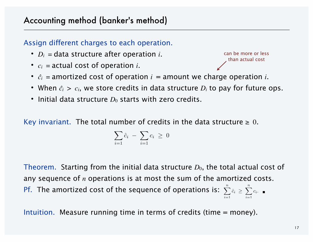
Accounting method (banker's method)
Assign different charges to each operation.
・Di = data structure after operation i.
・ci = actual cost of operation i.
・ĉi = amortized cost of operation i = amount we charge operation i.
・When ĉi > ci, we store credits in data structure Di to pay for future ops.
・Initial data structure D0 starts with zero credits.
Key invariant. The total number of credits in the data structure ≥ 0.
Theorem. Starting from the initial data structure D0, the total actual cost of
any sequence of n operations is at most the sum of the amortized costs.
Pf. The amortized cost of the sequence of operations is:
Intuition. Measure running time in terms of credits (time = money).
n�
i=1
ci �n�
i=1
ci. ▪
n�
i=1
ci �n�
i=1
ci � 0
can be more or lessthan actual cost
18
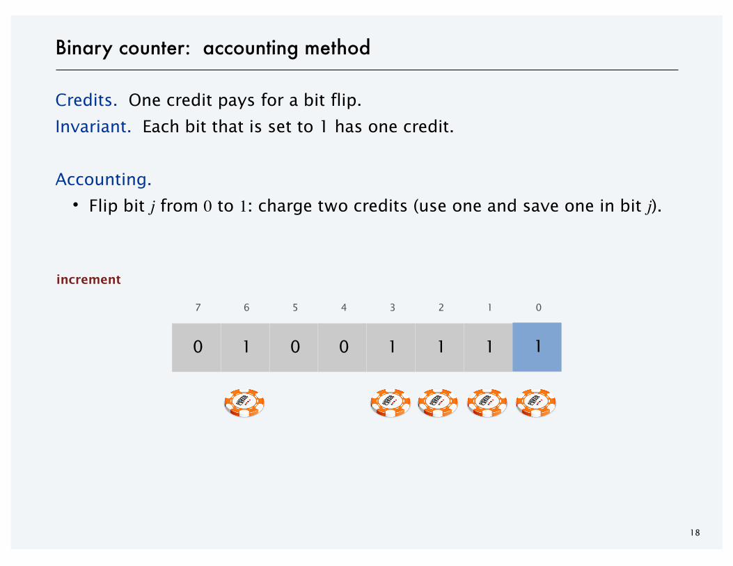
Binary counter: accounting method
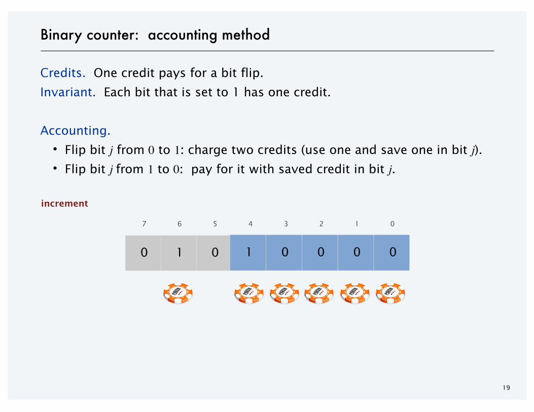
Credits. One credit pays for a bit flip.
Invariant. Each bit that is set to 1 has one credit.
Accounting.
・Flip bit j from 0 to 1: charge two credits (use one and save one in bit j).
7 6 5 4 3 2 1 0
0 1 0 0 1 1 1 0
increment
1
19
Binary counter: accounting method
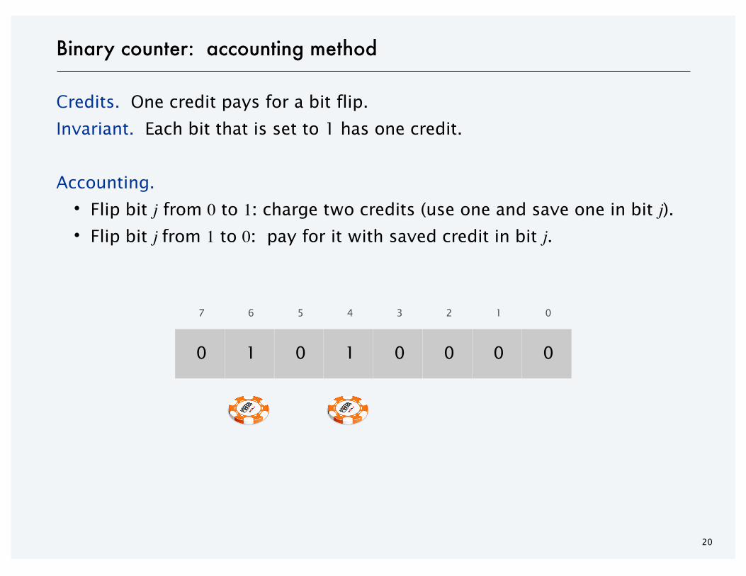
Credits. One credit pays for a bit flip.
Invariant. Each bit that is set to 1 has one credit.
Accounting.
・Flip bit j from 0 to 1: charge two credits (use one and save one in bit j).
・Flip bit j from 1 to 0: pay for it with saved credit in bit j.
7 6 5 4 3 2 1 0
0 1 0 0 1 1 1 1
increment
00001
20
Binary counter: accounting method
Credits. One credit pays for a bit flip.
Invariant. Each bit that is set to 1 has one credit.
Accounting.
・Flip bit j from 0 to 1: charge two credits (use one and save one in bit j).
・Flip bit j from 1 to 0: pay for it with saved credit in bit j.
7 6 5 4 3 2 1 0
0 1 0 1 0 0 0 0
21
Binary counter: accounting method
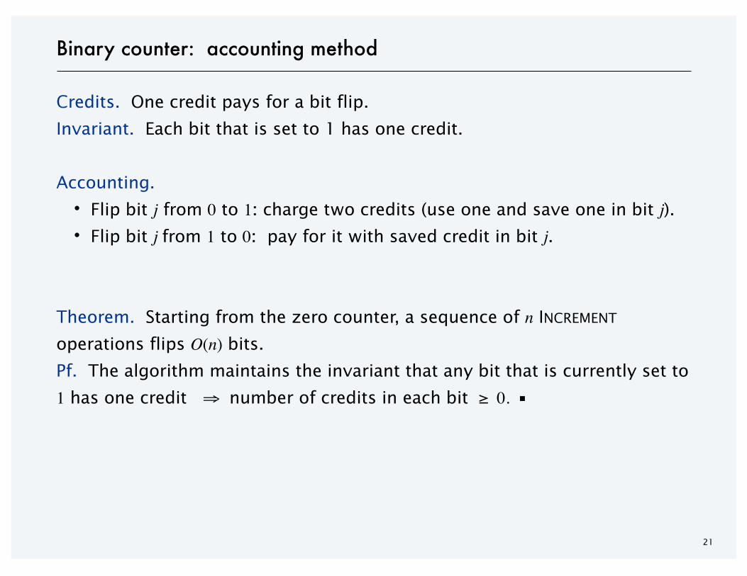
Credits. One credit pays for a bit flip.
Invariant. Each bit that is set to 1 has one credit.
Accounting.
・Flip bit j from 0 to 1: charge two credits (use one and save one in bit j).
・Flip bit j from 1 to 0: pay for it with saved credit in bit j.
Theorem. Starting from the zero counter, a sequence of n INCREMENT
operations flips O(n) bits.
Pf. The algorithm maintains the invariant that any bit that is currently set to
1 has one credit ⇒ number of credits in each bit ≥ 0. ▪
22
Potential method (physicist's method)
Potential function. Φ(Di) maps each data structure Di to a real number s.t.:
・Φ(D0) = 0.
・Φ(Di) ≥ 0 for each data structure Di.
Actual and amortized costs.
・ci = actual cost of ith operation.
・ĉi = ci + Φ(Di) – Φ(Di–1) = amortized cost of ith operation.
23
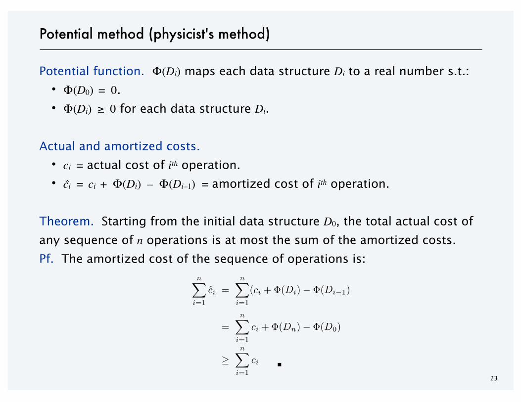
Potential method (physicist's method)
Potential function. Φ(Di) maps each data structure Di to a real number s.t.:
・Φ(D0) = 0.
・Φ(Di) ≥ 0 for each data structure Di.
Actual and amortized costs.
・ci = actual cost of ith operation.
・ĉi = ci + Φ(Di) – Φ(Di–1) = amortized cost of ith operation.
Theorem. Starting from the initial data structure D0, the total actual cost of
any sequence of n operations is at most the sum of the amortized costs.
Pf. The amortized cost of the sequence of operations is:n�
i=1
ci =n�
i=1
(ci + �(Di) � �(Di�1)
=n�
i=1
ci + �(Dn) � �(D0)
�n�
i=1
ci
n�
i=1
ci =n�
i=1
(ci + �(Di) � �(Di�1)
=n�
i=1
ci + �(Dn) � �(D0)
�n�
i=1
ci
n�
i=1
ci =n�
i=1
(ci + �(Di) � �(Di�1)
=n�
i=1
ci + �(Dn) � �(D0)
�n�
i=1
ci ▪
24
Binary counter: potential method
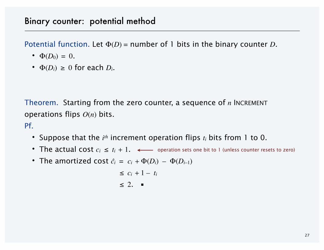
Potential function. Let Φ(D) = number of 1 bits in the binary counter D.
・Φ(D0) = 0.
・Φ(Di) ≥ 0 for each Di.
7 6 5 4 3 2 1 0
0 1 0 0 1 1 1 0
increment
1
25
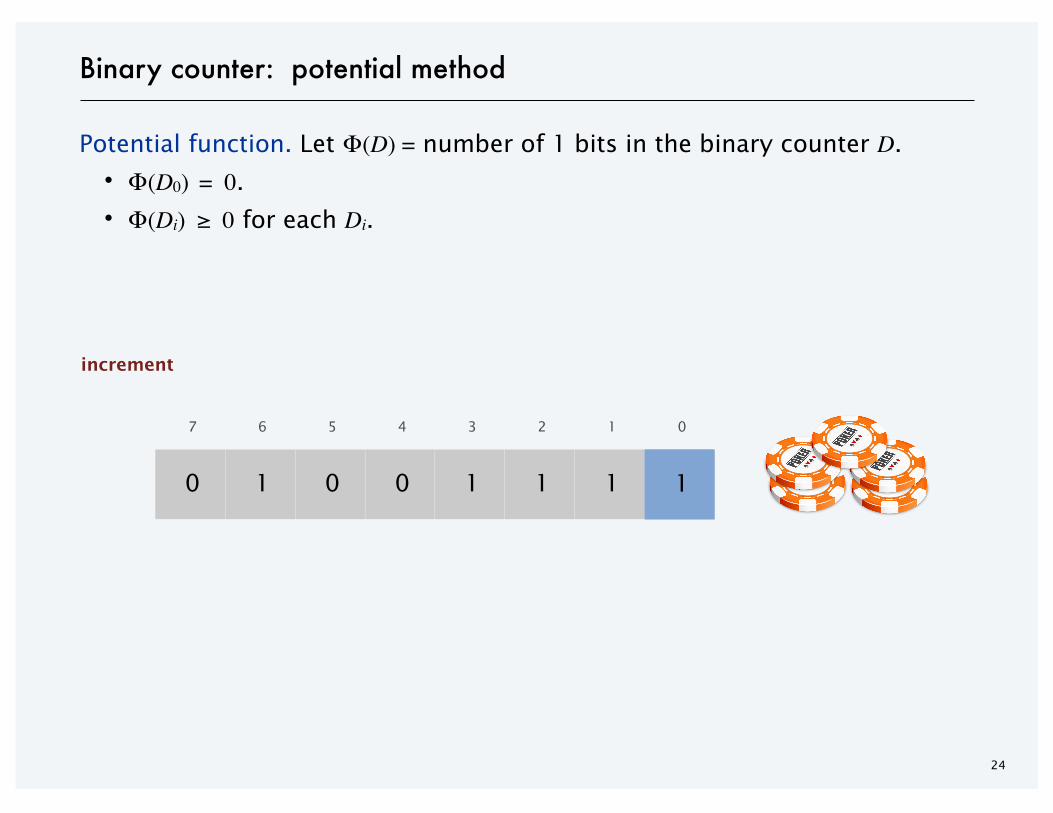
Binary counter: potential method
Potential function. Let Φ(D) = number of 1 bits in the binary counter D.
・Φ(D0) = 0.
・Φ(Di) ≥ 0 for each Di.
7 6 5 4 3 2 1 0
0 1 0 0 1 1 1 1
increment
00001
26
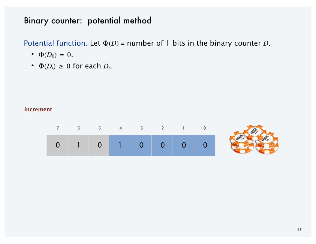
Binary counter: potential method
Potential function. Let Φ(D) = number of 1 bits in the binary counter D.
・Φ(D0) = 0.
・Φ(Di) ≥ 0 for each Di.
7 6 5 4 3 2 1 0
0 1 0 1 0 0 0 0
27
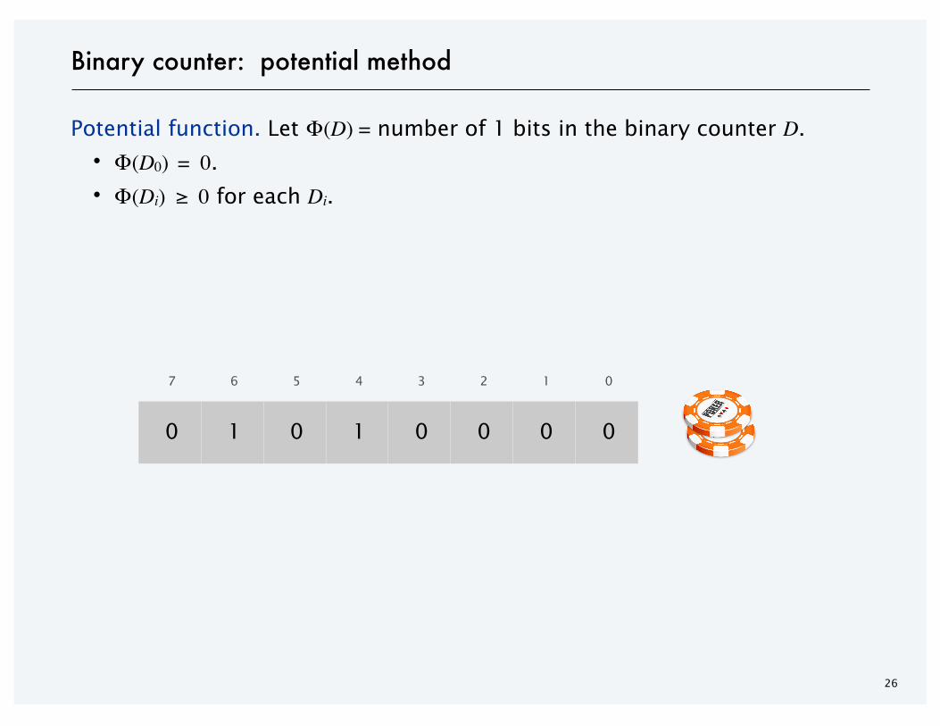
Binary counter: potential method
Potential function. Let Φ(D) = number of 1 bits in the binary counter D.
・Φ(D0) = 0.
・Φ(Di) ≥ 0 for each Di.
Theorem. Starting from the zero counter, a sequence of n INCREMENT
operations flips O(n) bits.
Pf.
・Suppose that the ith increment operation flips ti bits from 1 to 0.
・The actual cost ci ≤ ti + 1.
・The amortized cost ĉi = ci + Φ(Di) – Φ(Di–1) ≤ ci + 1 – ti
≤ 2. ▪
operation sets one bit to 1 (unless counter resets to zero)
28
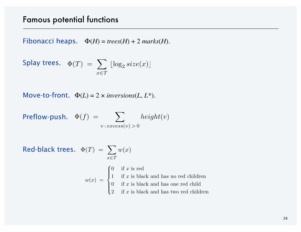
Famous potential functions
Fibonacci heaps. Φ(H) = trees(H) + 2 marks(H).
Splay trees.
Move-to-front. Φ(L) = 2 × inversions(L, L*).
Preflow-push.
Red-black trees. �(T ) =�
x�T
w(x)
w(x) =
�����
����
0 x
1 x
0 x
2 x
�(f) =�
v : excess(v) > 0
height(v)
�(T ) =�
x�T
�log2 size(x)�
SECTION 17.4
AMORTIZED ANALYSIS
‣ binary counter
‣ multipop stack
‣ dynamic table
30
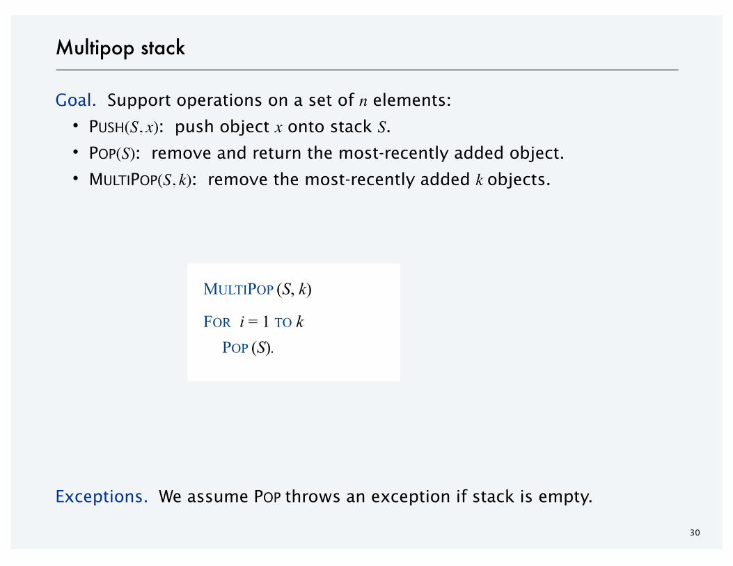
Multipop stack
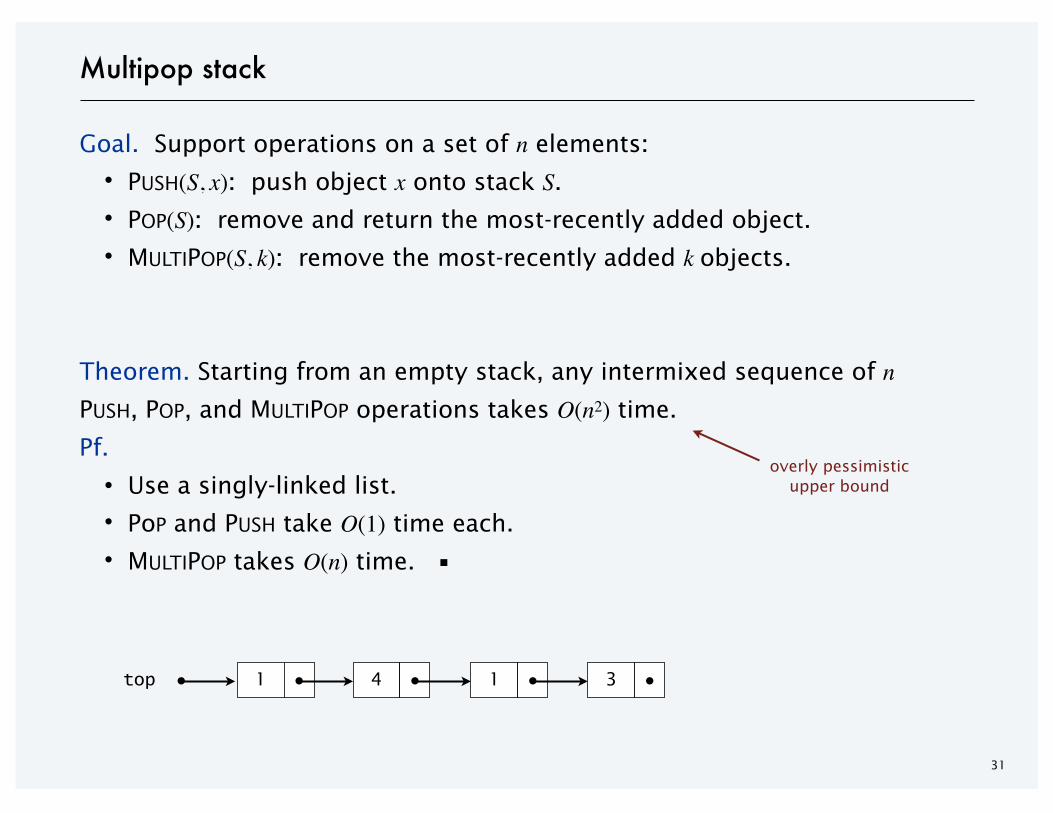
Goal. Support operations on a set of n elements:
・PUSH(S, x): push object x onto stack S.
・POP(S): remove and return the most-recently added object.
・MULTIPOP(S, k): remove the most-recently added k objects.
Exceptions. We assume POP throws an exception if stack is empty.
MULTIPOP (S, k) ___________________________________________________________________________________________________________________________________________________________________________________________________________________________________________________________________________________________________________________________________________________________________________________________________________________________________________________________________________________
FOR i = 1 TO k POP (S).
___________________________________________________________________________________________________________________________________________________________________________________________________________________________________________________________________________________________________________________________________________________________________________________________________________________________________________________________________________________
31
Multipop stack
Goal. Support operations on a set of n elements:
・PUSH(S, x): push object x onto stack S.
・POP(S): remove and return the most-recently added object.
・MULTIPOP(S, k): remove the most-recently added k objects.
Theorem. Starting from an empty stack, any intermixed sequence of nPUSH, POP, and MULTIPOP operations takes O(n2) time.
Pf.
・Use a singly-linked list.
・PoP and PUSH take O(1) time each.
・MULTIPOP takes O(n) time. ▪
overly pessimisticupper bound
1 ● 4 ● 1 ● 3 ●●top
32
Multipop stack: aggregate method
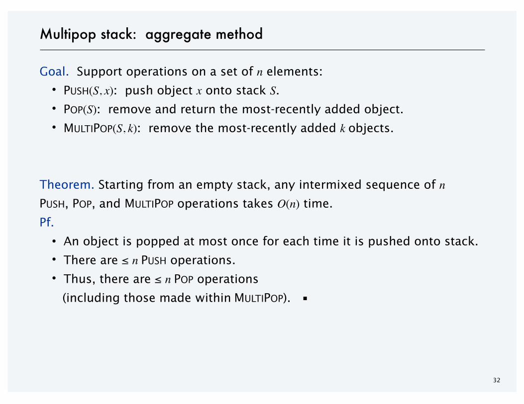
Goal. Support operations on a set of n elements:
・PUSH(S, x): push object x onto stack S.
・POP(S): remove and return the most-recently added object.
・MULTIPOP(S, k): remove the most-recently added k objects.
Theorem. Starting from an empty stack, any intermixed sequence of nPUSH, POP, and MULTIPOP operations takes O(n) time.
Pf.
・An object is popped at most once for each time it is pushed onto stack.
・There are ≤ n PUSH operations.
・Thus, there are ≤ n POP operations
(including those made within MULTIPOP). ▪
33
Multipop stack: accounting method
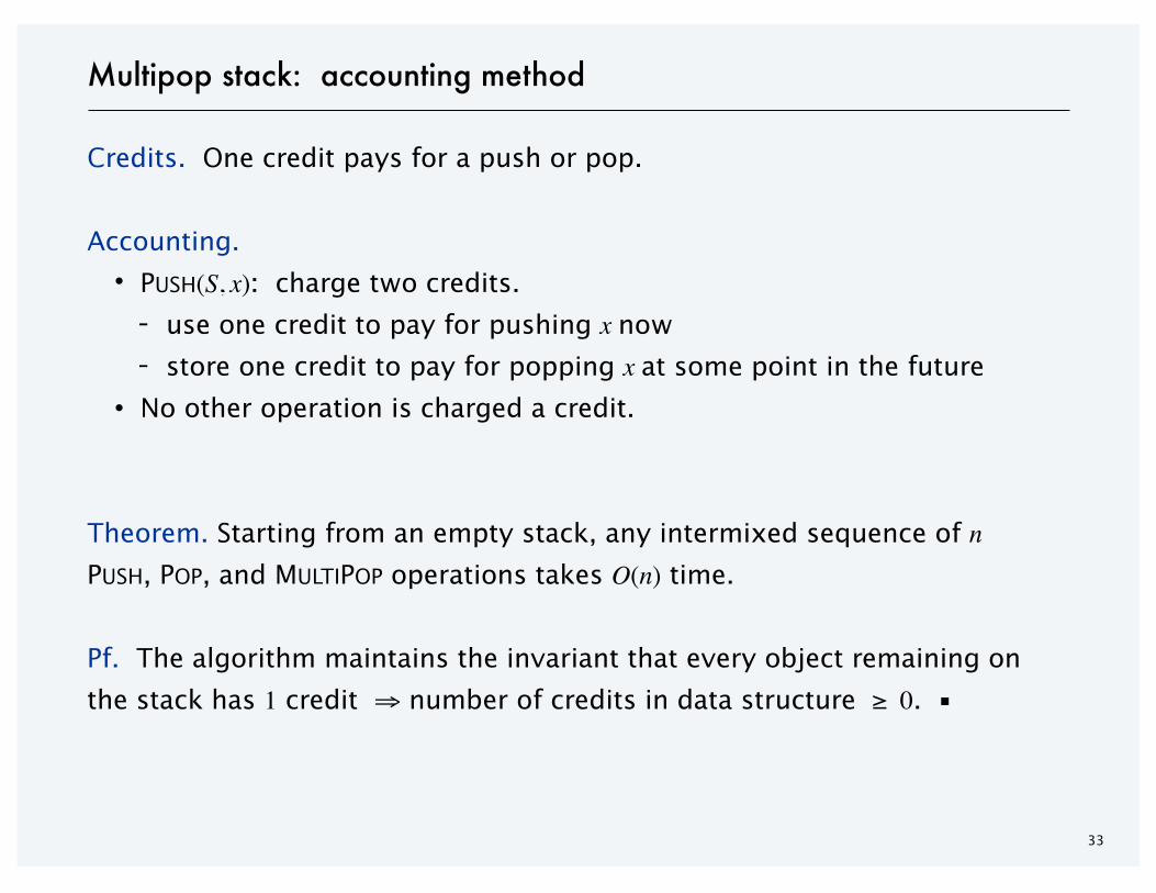
Credits. One credit pays for a push or pop.
Accounting.
・PUSH(S, x): charge two credits.- use one credit to pay for pushing x now- store one credit to pay for popping x at some point in the future
・No other operation is charged a credit.
Theorem. Starting from an empty stack, any intermixed sequence of nPUSH, POP, and MULTIPOP operations takes O(n) time.
Pf. The algorithm maintains the invariant that every object remaining on
the stack has 1 credit ⇒ number of credits in data structure ≥ 0. ▪
34
Multipop stack: potential method
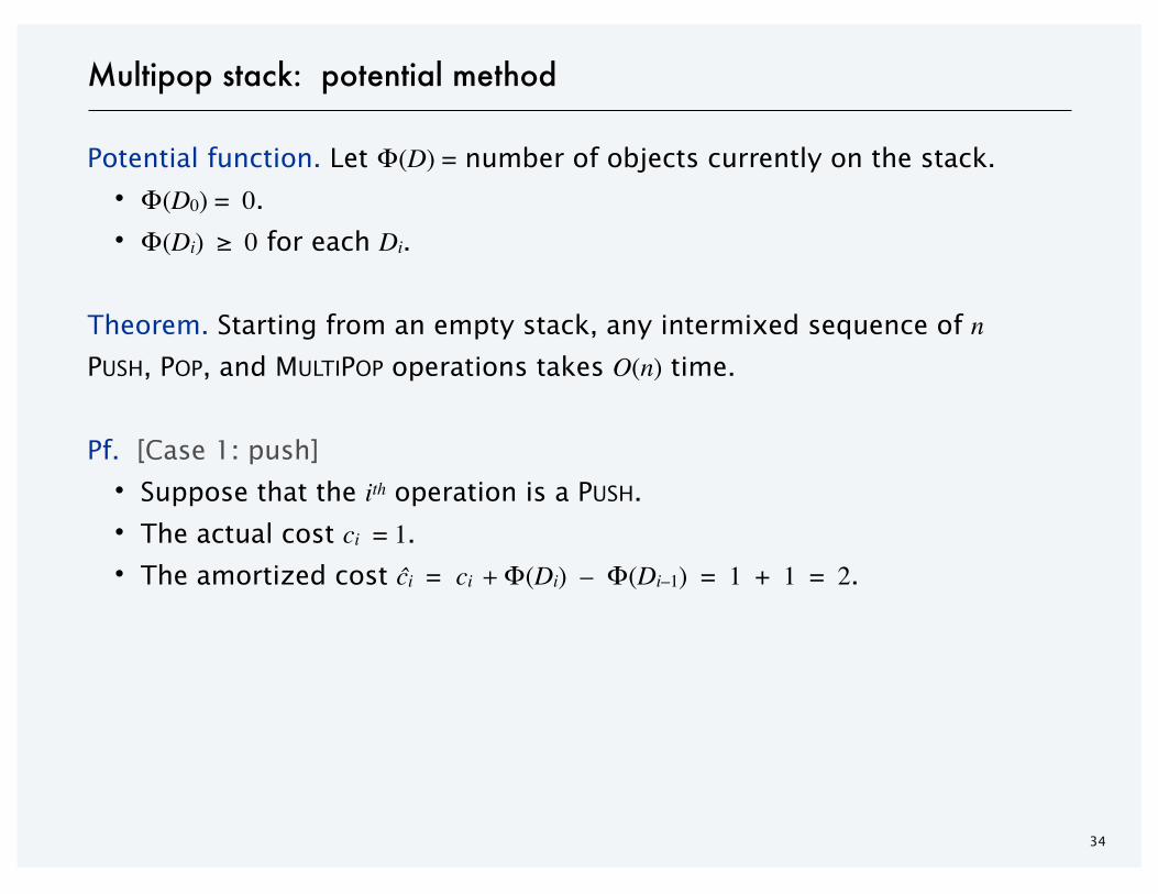
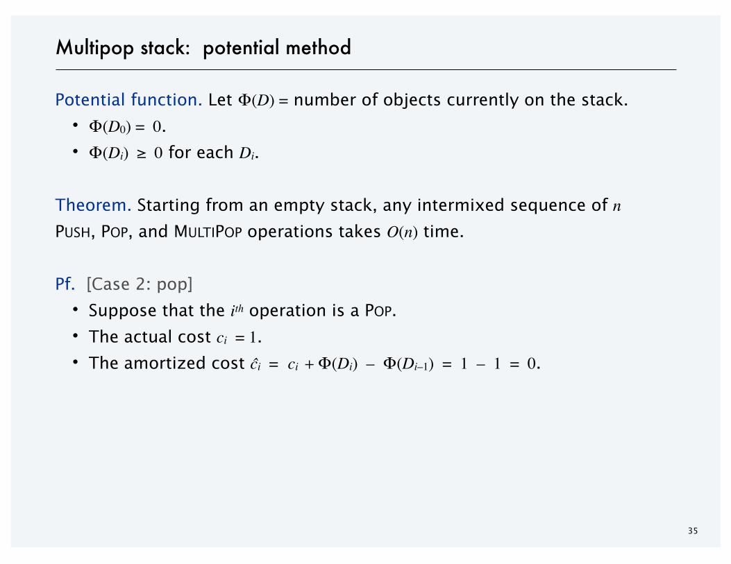
Potential function. Let Φ(D) = number of objects currently on the stack.
・Φ(D0) = 0.
・Φ(Di) ≥ 0 for each Di.
Theorem. Starting from an empty stack, any intermixed sequence of nPUSH, POP, and MULTIPOP operations takes O(n) time.
Pf. [Case 1: push]
・Suppose that the ith operation is a PUSH.
・The actual cost ci = 1.
・The amortized cost ĉi = ci + Φ(Di) – Φ(Di–1) = 1 + 1 = 2.
35
Multipop stack: potential method
Potential function. Let Φ(D) = number of objects currently on the stack.
・Φ(D0) = 0.
・Φ(Di) ≥ 0 for each Di.
Theorem. Starting from an empty stack, any intermixed sequence of nPUSH, POP, and MULTIPOP operations takes O(n) time.
Pf. [Case 2: pop]
・Suppose that the ith operation is a POP.
・The actual cost ci = 1.
・The amortized cost ĉi = ci + Φ(Di) – Φ(Di–1) = 1 – 1 = 0.
36
Multipop stack: potential method
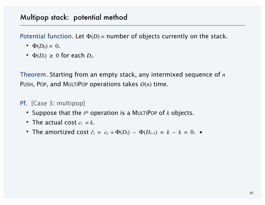
Potential function. Let Φ(D) = number of objects currently on the stack.
・Φ(D0) = 0.
・Φ(Di) ≥ 0 for each Di.
Theorem. Starting from an empty stack, any intermixed sequence of nPUSH, POP, and MULTIPOP operations takes O(n) time.
Pf. [Case 3: multipop]
・Suppose that the ith operation is a MULTIPOP of k objects.
・The actual cost ci = k.
・The amortized cost ĉi = ci + Φ(Di) – Φ(Di–1) = k – k = 0. ▪
SECTION 17.4
AMORTIZED ANALYSIS
‣ binary counter
‣ multipop stack
‣ dynamic table
38
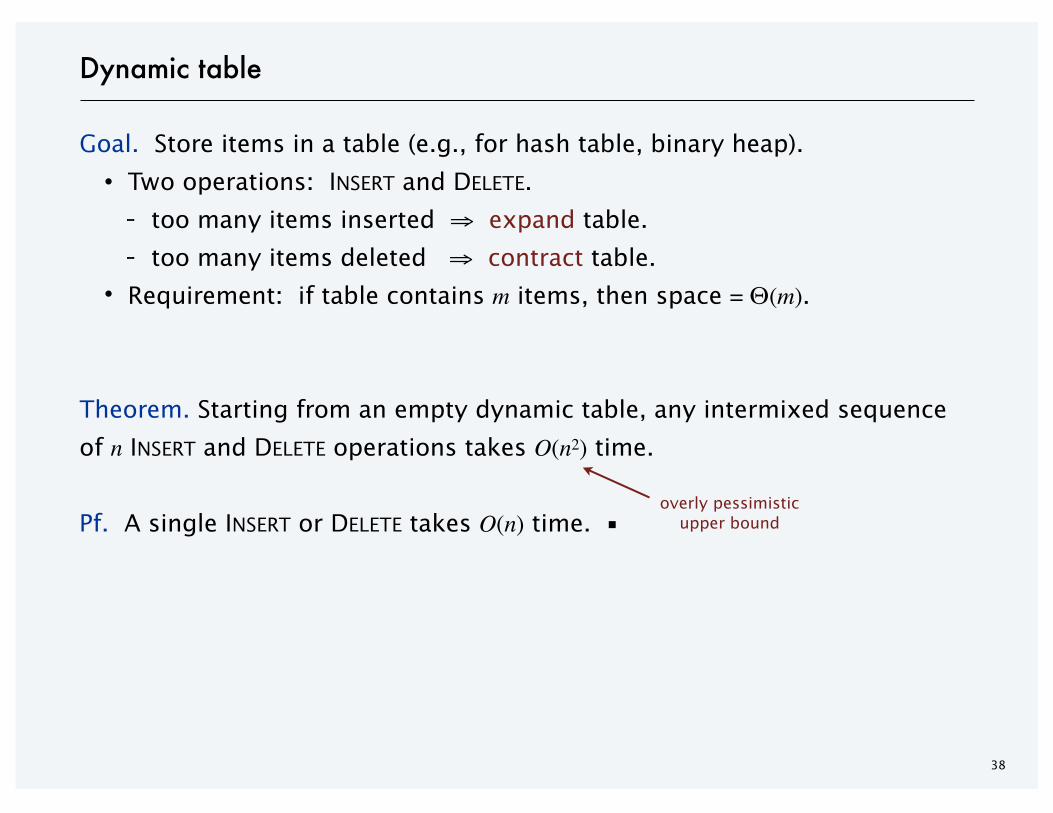
Dynamic table
Goal. Store items in a table (e.g., for hash table, binary heap).
・Two operations: INSERT and DELETE.- too many items inserted ⇒ expand table.- too many items deleted ⇒ contract table.
・Requirement: if table contains m items, then space = Θ(m).
Theorem. Starting from an empty dynamic table, any intermixed sequence
of n INSERT and DELETE operations takes O(n2) time.
Pf. A single INSERT or DELETE takes O(n) time. ▪overly pessimistic
upper bound
39
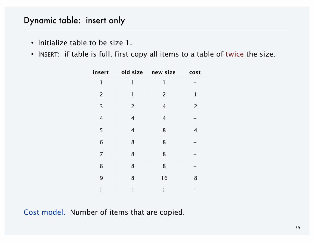
・Initialize table to be size 1.
・INSERT: if table is full, first copy all items to a table of twice the size.
Cost model. Number of items that are copied.
Dynamic table: insert only
insert old size new size cost
1 1 1 –
2 1 2 1
3 2 4 2
4 4 4 –
5 4 8 4
6 8 8 –
7 8 8 –
8 8 8 –
9 8 16 8
⋮ ⋮ ⋮ ⋮
40
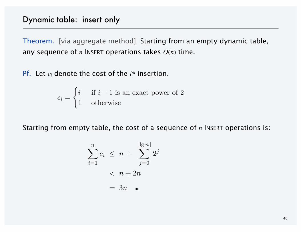
Theorem. [via aggregate method] Starting from an empty dynamic table,
any sequence of n INSERT operations takes O(n) time.
Pf. Let ci denote the cost of the ith insertion.
Starting from empty table, the cost of a sequence of n INSERT operations is:
Dynamic table: insert only
n�
i=1
ci � n +
�lg n��
j=0
2j
< n + 2n
= 3n
ci =
�i i � 1
1
▪
n�
i=1
ci � n +
�lg n��
j=0
2j
< n + 2n
= 3n
n�
i=1
ci � n +
�lg n��
j=0
2j
< n + 2n
= 3n
1 2 3 4 5 6 7 8
1 2 3 4
41
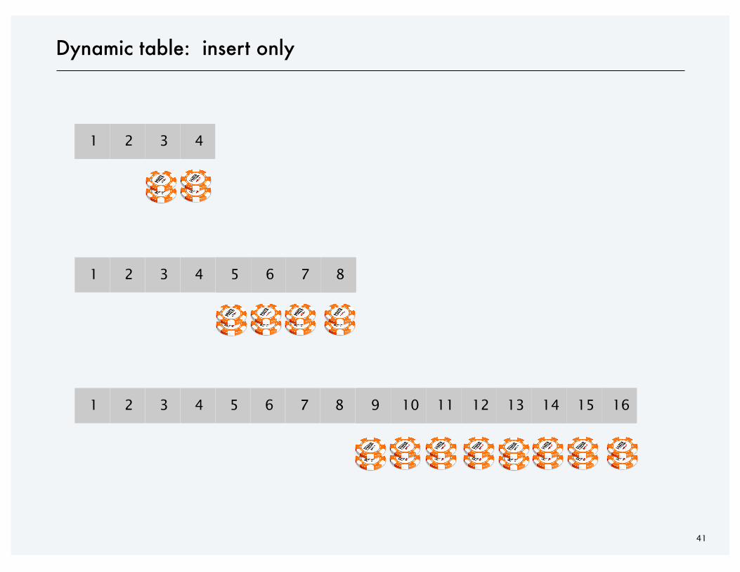
Dynamic table: insert only
5 6 7 8
9 10 11 12 13 14 15 16
1 2 3 4
42
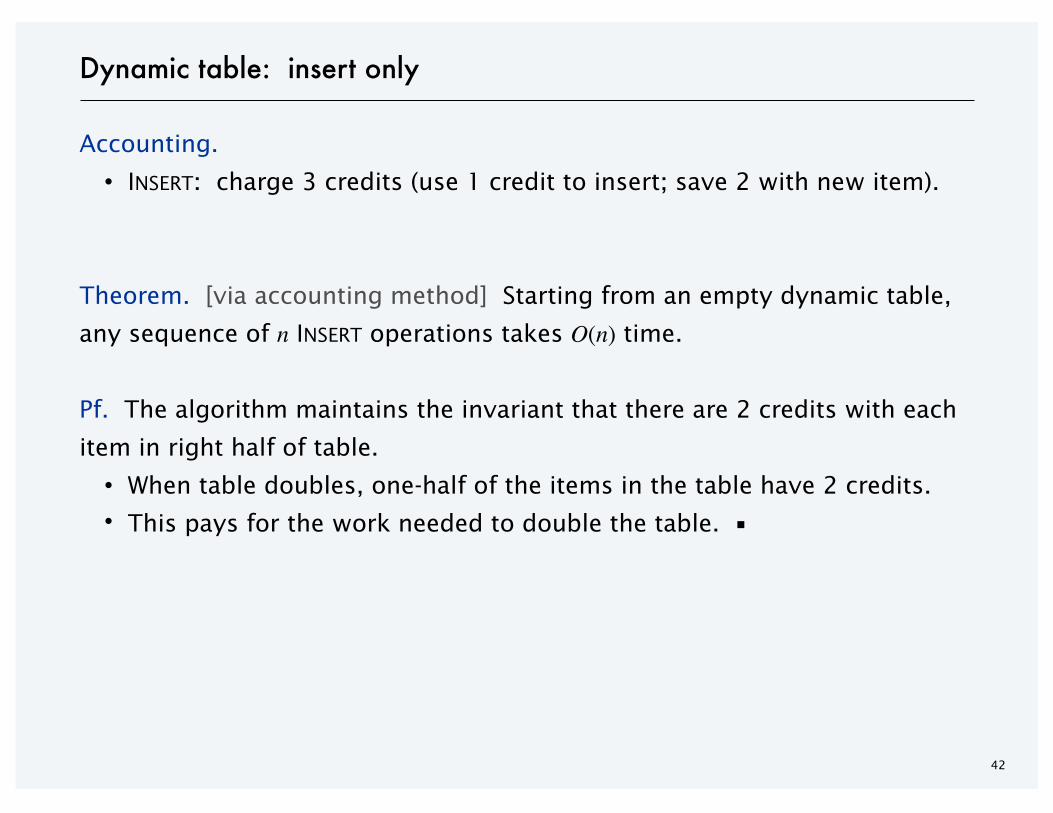
Accounting.
・INSERT: charge 3 credits (use 1 credit to insert; save 2 with new item).
Theorem. [via accounting method] Starting from an empty dynamic table,
any sequence of n INSERT operations takes O(n) time.
Pf. The algorithm maintains the invariant that there are 2 credits with each
item in right half of table.
・When table doubles, one-half of the items in the table have 2 credits.
・This pays for the work needed to double the table. ▪
Dynamic table: insert only
43
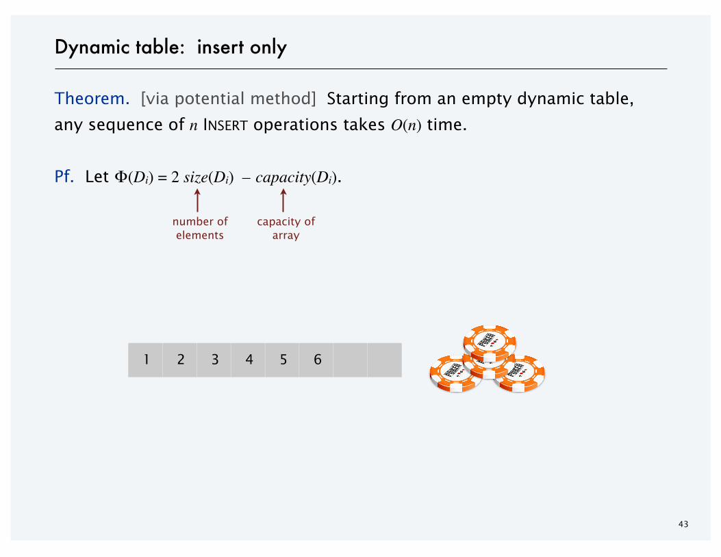
Theorem. [via potential method] Starting from an empty dynamic table,
any sequence of n INSERT operations takes O(n) time.
Pf. Let Φ(Di) = 2 size(Di) – capacity(Di).
Dynamic table: insert only
number ofelements
capacity ofarray
1 2 3 4 5 6
44
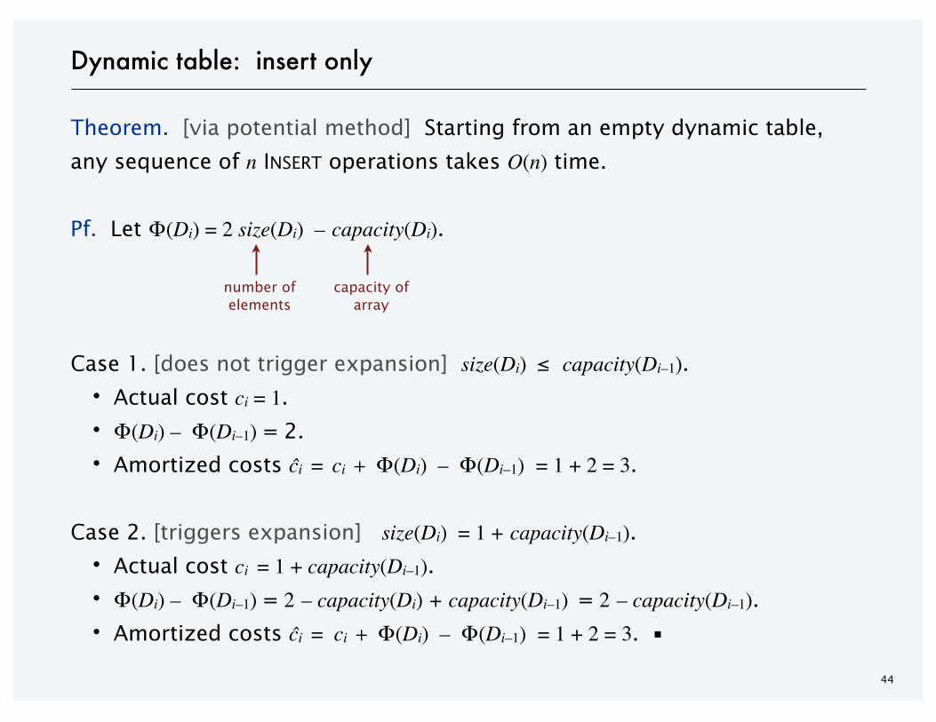
Theorem. [via potential method] Starting from an empty dynamic table,
any sequence of n INSERT operations takes O(n) time.
Pf. Let Φ(Di) = 2 size(Di) – capacity(Di).
Case 1. [does not trigger expansion] size(Di) ≤ capacity(Di–1).
・Actual cost ci = 1.
・Φ(Di) – Φ(Di–1) = 2.
・Amortized costs ĉi = ci + Φ(Di) – Φ(Di–1) = 1 + 2 = 3.
Case 2. [triggers expansion] size(Di) = 1 + capacity(Di–1).
・Actual cost ci = 1 + capacity(Di–1).
・Φ(Di) – Φ(Di–1) = 2 – capacity(Di) + capacity(Di–1) = 2 – capacity(Di–1).
・Amortized costs ĉi = ci + Φ(Di) – Φ(Di–1) = 1 + 2 = 3. ▪
Dynamic table: insert only
number ofelements
capacity ofarray
45
Dynamic table: doubling and halving
Thrashing.
・Initialize table to be of fixed size, say 1.
・INSERT: if table is full, expand to a table of twice the size.
・DELETE: if table is ½-full, contract to a table of half the size.
Efficient solution.
・Initialize table to be of fixed size, say 1.
・INSERT: if table is full, expand to a table of twice the size.
・DELETE: if table is ¼-full, contract to a table of half the size.
Memory usage. A dynamic table uses O(n) memory to store n items.
Pf. Table is always at least ¼-full (provided it is not empty). ▪

46
Dynamic table: insert and delete
Theorem. [via aggregate method] Starting from an empty dynamic table,
any intermixed sequence of n INSERT and DELETE operations takes O(n) time.
Pf.
・In between resizing events, each INSERT and DELETE takes O(1) time.
・Consider total amount of work between two resizing events.- Just after the table is doubled to size m, it contains m / 2 items.- Just after the table is halved to size m, it contains m / 2 items.- Just before the next resizing, it contains either m / 4 or 2 m items.- After resizing to m, we must perform Ω(m) operations before we resize
again (either ≥ m insertions or ≥ m / 4 deletions).
・Resizing a table of size m requires O(m) time. ▪
47
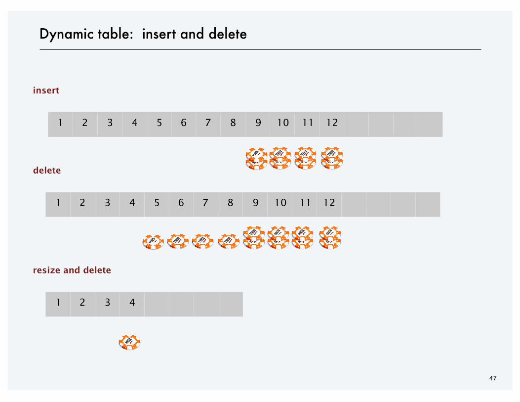
Dynamic table: insert and delete
121110987654321
insert
1110987654321
delete
12
4321
resize and delete
48
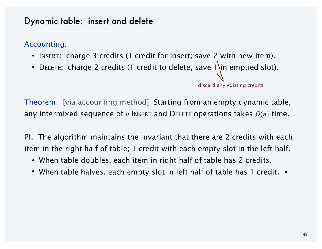
Accounting.
・INSERT: charge 3 credits (1 credit for insert; save 2 with new item).
・DELETE: charge 2 credits (1 credit to delete, save 1 in emptied slot).
Theorem. [via accounting method] Starting from an empty dynamic table,
any intermixed sequence of n INSERT and DELETE operations takes O(n) time.
Pf. The algorithm maintains the invariant that there are 2 credits with each
item in the right half of table; 1 credit with each empty slot in the left half.
・When table doubles, each item in right half of table has 2 credits.
・When table halves, each empty slot in left half of table has 1 credit. ▪
Dynamic table: insert and delete
discard any existing credits
49
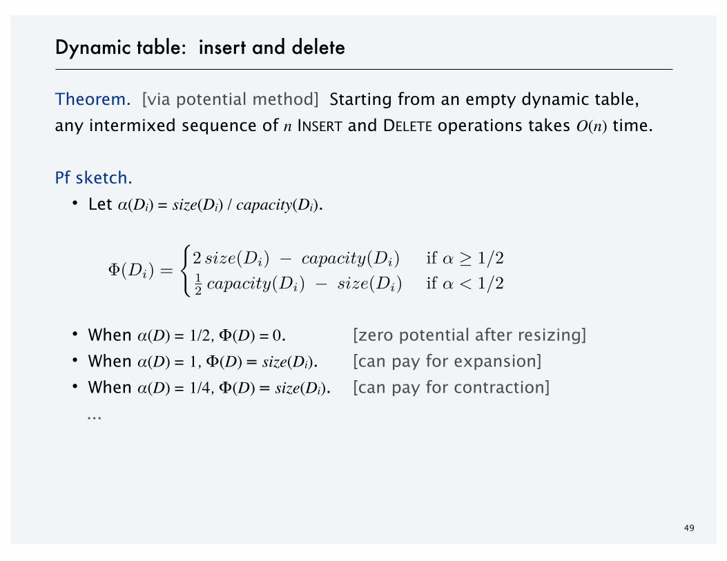
Theorem. [via potential method] Starting from an empty dynamic table,
any intermixed sequence of n INSERT and DELETE operations takes O(n) time.
Pf sketch.
・Let α(Di) = size(Di) / capacity(Di).
・When α(D) = 1/2, Φ(D) = 0. [zero potential after resizing]
・When α(D) = 1, Φ(D) = size(Di). [can pay for expansion]
・When α(D) = 1/4, Φ(D) = size(Di). [can pay for contraction]
...
Dynamic table: insert and delete
�(Di) =
�2 size(Di) � capacity(Di) � � 1/212 capacity(Di) � size(Di) � < 1/2