This content has been downloaded from IOPscience. Please scroll down to see the full text.

Download details:

IP Address: 128.112.40.231

This content was downloaded on 08/06/2017 at 21:20

Please note that terms and conditions apply.

Amplification of flood frequencies with local sea level rise and emerging flood regimes

View the table of contents for this issue, or go to the journal homepage for more

2017 Environ. Res. Lett. 12 064009

(http://iopscience.iop.org/1748-9326/12/6/064009)

Home Search Collections Journals About Contact us My IOPscience

You may also be interested in:

Modelling sea level rise impacts on storm surges along US coasts

Claudia Tebaldi, Benjamin H Strauss and Chris E Zervas

A multi-dimensional integrated approach to assess flood risks on a coastal city, induced by

sea-level rise and storm tides

Xu Lilai, He Yuanrong, Huang Wei et al.

US power plant sites at risk of future sea-level rise

R Bierkandt, M Auffhammer and A Levermann

The exceptional influence of storm ‘Xaver’ on design water levels in the German Bight

Sönke Dangendorf, Arne Arns, Joaquim G Pinto et al.

Comparing hurricane and extratropical storm surge for the Mid-Atlantic and Northeast Coast of the

United States for 1979–2013

J F Booth, H E Rieder and Y Kushnir

Climate change effects on the worst-case storm surge: a case study of Typhoon Haiyan

Izuru Takayabu, Kenshi Hibino, Hidetaka Sasaki et al.

The co-incidence of storm surges and extreme discharges within the Rhine–Meuse Delta

W J Klerk, H C Winsemius, W J van Verseveld et al.

Bounding probabilistic sea-level projections within the framework of the possibility theory

Gonéri Le Cozannet, Jean-Charles Manceau and Jeremy Rohmer

Estimating 21st century changes in extreme sea levels around Western Australia

I D Haigh and C Pattiaratchi

OPEN ACCESS

RECEIVED

14 February 2017

REVISED

20 March 2017

ACCEPTED FOR PUBLICATION

12 April 2017

PUBLISHED

7 June 2017

Original content fromthis work may be usedunder the terms of theCreative CommonsAttribution 3.0 licence.

Any further distributionof this work mustmaintain attribution tothe author(s) and thetitle of the work, journalcitation and DOI.

Environ. Res. Lett. 12 (2017) 064009 https://doi.org/10.1088/1748-9326/aa6cb3

LETTER

Amplification of flood frequencies with local sea level rise andemerging flood regimes

Maya K Buchanan1,4, Michael Oppenheimer1,2 and Robert E Kopp3

1 Woodrow Wilson School of Public and International Affairs, Princeton University, Princeton, NJ, United States of America2 Department of Geosciences, Princeton University, Princeton, NJ, United States of America3 Department of Earth and Planetary Sciences, Rutgers Energy Institute, and Institute of Earth, Ocean, and Atmospheric Sciences,

Rutgers University, New Brunswick, NJ, United States of America4 Author to whom any correspondence should be addressed.

E-mail: mayakb@princeton.edu

Keywords: sea level rise, coastal flooding, climate change impacts, deep uncertainty, extreme value theory, risk management

Supplementary material for this article is available online

AbstractThe amplification of flood frequencies by sea level rise (SLR) is expected to become one of themost economically damaging impacts of climate change for many coastal locations.Understanding the magnitude and pattern by which the frequency of current flood levels increaseis important for developing more resilient coastal settlements, particularly since flood riskmanagement (e.g. infrastructure, insurance, communications) is often tied to estimates of floodreturn periods. The Intergovernmental Panel on Climate Change’s Fifth Assessment Reportcharacterized the multiplication factor by which the frequency of flooding of a given heightincreases (referred to here as an amplification factor; AF). However, this characterization neitherrigorously considered uncertainty in SLR nor distinguished between the amplification of differentflooding levels (such as the 10% versus 0.2% annual chance floods); therefore, it may beseriously misleading. Because both historical flood frequency and projected SLR are uncertain, wecombine joint probability distributions of the two to calculate AFs and their uncertainties overtime. Under probabilistic relative sea level projections, while maintaining storm frequency fixed,we estimate a median 40-fold increase (ranging from 1- to 1314-fold) in the expected annualnumber of local 100-year floods for tide-gauge locations along the contiguous US coastline by2050. While some places can expect disproportionate amplification of higher frequency eventsand thus primarily a greater number of historically precedented floods, others face amplificationof lower frequency events and thus a particularly fast growing risk of historically unprecedentedflooding. For example, with 50 cm of SLR, the 10%, 1%, and 0.2% annual chance floods areexpected respectively to recur 108, 335, and 814 times as often in Seattle, but 148, 16, and 4times as often in Charleston, SC.

1. Introduction

Coastal flooding is already one of the most damagingenvironmental hazards—responsible for a great lossof life, property, and long-term effects on municipalservices and economic health (Hsiang and Jina 2014,USACE 2015). Flood height is driven by sea level rise(SLR) and storm tide, which in turn is composed oftide and storm surge. Even a small amount of SLRaugments the flood height associated with a storm

© 2017 IOP Publishing Ltd

surge or tidal event. Indeed, flooding amplified bySLR is projected to be the most damaging marketimpact of climate change for many coastal regions ofthe US in the 21st century (Houser et al 2015).Understanding the magnitude and pattern by whichthe frequency of current flood levels (such as the 1%annual chance flood, or equivalently the 100-yearflood) increase is critical for developing more resilientcoastal areas, particularly since coastal infrastructuremanagement, federal flood insurance, and flood risk

Environ. Res. Lett. 12 (2017) 064009

communications are typically tied to estimates offlood return periods (e.g. NYC 2013, Douglas et al2016).

The amplification factor (AF) is a metric thatmeasures the change in the expected frequency of ahistoric annual chance flood with SLR. It has beencalculated explicitly (Hunter 2012, Church et al2013) and implicitly (by estimating changes in floodfrequency; Tebaldi et al 2012, Lin et al 2012) to aidstakeholder decision-making about coastal floodrisk management. AFs are a function of thefrequency distribution of storm tide events andthe amount of local SLR—both of which areuncertain (see section 3). Storm tide distributionscan be simulated with hydrodynamic models, whichmay then be fit by an extreme value distribution toestimate the storm tide frequency distribution(including or excluding SLR, e.g. Lin et al 2012and Muis et al 2016, respectively). Alternatively,observations can be fit to an extreme valuedistribution to estimate a storm tide distribution,which can be adjusted for the distribution of futureSLR. Extreme value theory is commonly usedbecause of the computational intensity of high-resolution hydrodynamic modeling and also becauseit is data-based, capturing both tropical and non-tropical storm surges. Although hydrodynamicmodeling can simulate potential changes in stormsurges associated with tropical cyclones in responseto warming sea surface temperatures and changingwind patterns, there is low confidence in climatemodel projections of future tropical cyclone behav-ior, particularly in individual basins (e.g. Knutsonet al 2010). Here, we assume there are no significantchanges in tides or storm climatology that wouldaffect storm tide distributions.

The Gumbel extreme value distribution wasprominently used in the Intergovernmental Panelon Climate Change’s (IPCC) Fifth Assessment Report(AR5; Church et al 2013) and elsewhere (Hunter2012, Muis et al 2016) because it has the advantage ofsimplicity, assuming an exponential relationshipbetween the level and frequency of flooding.However, AFs estimated by it are invariant to floodlevels and do not capture the distinct effects of SLR onflooding in areas with heavy- and thin-tailed floodfrequency distributions. Here we present calculationsof the amplification of flood return periods usingextreme value theory allowing for heavy- and thin-tailed distributions and their change with SLR. Wecombine joint probability distributions of floodfrequency using the Generalized Pareto Distribution(GPD), incorporating uncertainty in this extremevalue distribution and employing probabilistic localSLR projections (conditional upon a greenhouse gasemissions pathway) to provide AFs along US coast-lines for various flood levels, timeframes, and SLRscenarios.

2

2. Estimating the amplification of floodfrequencies

There are two main families of extreme valuedistributions: the Generalized Extreme Value (GEV)distribution and GPD. The GEV family of distribu-tions is used in block maxima analysis, in whichextremes are estimated by maximum water levels overa unit of time (e.g. annual values). The GPD is used inpeak-over-threshold (POT) analysis, in which theprobability of having an event over a specifiedthreshold is described by a Poission distributionand the GPD characterizes the conditional probabilityof an event of a given magnitude. In a POTanalysis, allobservations over a high threshold (e.g. the 99thpercentile of hourly water levels; Tebaldi et al 2012) areused to estimate the distribution of flood events (e.g.water level extremes). Hence, the GPD incorporatessub-annual maxima, making use of more of theavailable data. For these reasons, the GPD has beenrecognized as a hydrological standard since 1975(NERC 1975, Coles et al 2001).

The number of exceedances of flood level z for theGEV and Poisson–GPD are given by:

NðzÞ ¼λ 1þ jðz � mÞ

s

� ��1

j for j≠ 0

λ exp � z � m

s

� �for j ¼ 0

8>>>>><>>>>>:

ð1Þ

whereby the distributions are characterized by location(m), scale (s), and shape (j) parameters. The locationparameter relates to local sea level, the scale parameterto the variability in the maxima of water level causedby the combination of tides and storm surges, and theshape parameter to the curvature and upward limit ofa flood frequency curve. These expressions for thenumber of exceedances in the GEVand Poisson–GPDare identical except for λ. For the Poisson–GPD, λ isthe Poisson-distributed annual mean number of floodevents; for a GEV describing annual block maxima,λ ¼ 1 event/year (Hunter 2012, Buchanan et al 2016).For j ¼ 0, the expression is identical to that for aGumbel distribution, a simple exponential function(figure 1(a)).

The shape parameter dominates the tail of a floodfrequency distribution (Coles et al 2001), illustrated bythe distinction between curves in figure 1(a) from onlya variation in j, holding all other parameters constant.Flood frequency distributions with j > 0 are ‘heavy-tailed’, with a relatively high frequency of extremeflood levels. Conversely, flood frequency curves withj< 0 are ‘thin-tailed’, having an upper bound ofextreme flood levels.

0 200 400 600 800 1000

Amplification factor offlood return periods

return period, 1/N(z)

AF

(z)

0.5 1.0 1.5 2.0

Flood levelfrequency

z (meters)

N (

z)

0.5 1.0 1.5 2.0

Amplification factor offlood levels

z (meters)

AF

(z)

> 0 < 0 = 0

a b c

103

101

10-1

10-2

10-4

103

101

10-1

Figure 1. (a) Flood frequency distributions (the number of expected events of flood level z), (b) amplification factors (AFs) of floodlevels z, and (c) AFs of corresponding return periods (1 / N(z)) for 0.5m SLR and three hypothetical GPD curves with equalparameters except for varying shape factors (j). The green, blue and black lines correspond to a positive (j ¼ .15), negative(j ¼ � .15), and zero j. The AF of a given flood level z is dependent on the sign of the extreme value shape parameter.

Environ. Res. Lett. 12 (2017) 064009

The AF of a flood of height z after SLR is N(z � d)/N (z), where N (z � d) is the new expectednumber of exceedances of the flood level with SLR:

AFðzÞ ¼ Nðz � dÞNðzÞ

¼ 1� d

ðs=jÞ þ z � m

� ��1

j for j≠ 0

exp d

s

� �for j ¼ 0

8>>>><>>>>:

ð2Þ

Taking the derivative of AF(z) with respect to z showsthe dependence of the AF on flood height:

@AFðzÞ@z

¼�dj½AFðzÞ�ð1þjÞ

ðjðz � mÞ þ sÞ for j≠ 0

0 for j ¼ 0

8<: ð3Þ

Assuming AF(z) and d > 0, the sign of ∂AF(z) /∂z isequal to the sign of �j, so the AF is decreasing withflood height for positive shape factors and increasingwith flood height for negative shape factors (figures 1(b) and (c)).

For j ¼ 0 (i.e. a Gumbel distribution), ∂AF(z) / ∂z¼ 0; there is no dependence of AF on flood height, andthus its use assumes AFs are invariant to flood levels;i.e. that all flood frequencies amplify by the samemagnitude (figures 1(b) and (c)). A key question thusarises among the approaches in extreme value theoryto fit a distribution to flood frequencies—whether touse the simple Gumbel distribution or the GPD/GEVthat requires fitting of a shape parameter. Because theshape parameter is dominant in determining a floodfrequency distribution, there is a trade-off between thesimplicity of the extreme value distribution used andits validity (Coles et al 2001). Simple approximationsare more tractable numerically; however, they aresuboptimal when another accessible approach candifferentiate between varying values of key metrics ofconcern—such as changes in the recurrence of the10-year vs 500-year flood under climate change.

Amplification of flooding frequency is also heavilyinfluenced by how local SLR is characterized. Underuncertain SLR, the AF equals E[(N (z)� d) /N (z)]. By

3

Jensen’s inequality (Jensen 1906), the convex trans-formation of the expectation of a random variable isless than or equal to the expectation of the convextransformation of the random variable. As a result ofJensen’s inequality and the approximate log-linearityof flood frequency curves, the AF under expected SLRis less than the expected AF under uncertain SLR, suchthat E[(N (z) � d)/N(z)] � N (z � E[d])/N(z). Thisinequality holds even if the distribution of SLR issymmetric, and the discrepancy is larger still if thedistribution is positively skewed (i.e. when expectedSLR is greater than median SLR). Because N(z) is alsoa random variable, accounting for the uncertainty inthe extreme value distribution fit is also important.

3. Methods

3.1. Extreme value theoryWe analyze National Oceanic and AtmosphericAdministration (NOAA) hourly tide-gauge recordsfor sites with a minimum 30 year record (which can befound at http://tidesandcurrents.noaa.gov/) followingthe methodology of Tebaldi et al (2012) and Buchananet al (2016). The GPD is estimated using hourly waterlevel exceedances above a high threshold (equal to the99th percentile of the hourly water level; Gilleland andKatz 2011). Hourly tide records are used to capturestorm surge, astronomical tides, and interannual sealevel variability, and are detrended to remove thecontribution of changes in mean sea level. To accountfor uncertainty in fit, GPD parameters are estimatedby maximum likelihood, and their covariance isestimated based on the observed Fisher informationmatrix (the Hessian of the negative log-likelihood atthe maximum-likelihood estimate). We sample 1000parameter pairs with Latin hypercube sampling,assuming the parameter uncertainty is normallydistributed. The expected number of exceedancesunder parameter uncertainty is calculated for ourmain calculations. Below the GPD threshold ofλ events per year, we fit a Gumbel distribution with182.6 events exceeding mean higher high water(MHHW) per year, assuming about half of all dayshave higher high water levels above mean higher high

Environ. Res. Lett. 12 (2017) 064009

water. For a comparative analysis, a Gumbel distribu-tion is also fitted to the full distribution of thresholdexceedances.

3.2. Sea level rise projectionsWeuse10 000MonteCarlo samples ofKopp et al (2014)local SLR projections, accounting for global and localcontributions, including land subsidence,distributionaleffects of land-ice melt (SLR fingerprints), and expertassessment of dynamic ice-sheet collapse. These SLRprojections are asymmetric, and—due primarily to thepoorly constrained but potentially large contribution ofthe Antarctic ice sheet (e.g. DeConto and Pollard 2016)—positively skewed. We use two RepresentativeConcentration Pathways (RCP) 4.5 and 8.5 whichrepresent greenhouse gas concentrations that lead to aradiative forcing of 4.5 and 8.5 W m�2 by 2100 (VanVuuren et al 2011).

3.3. Amplification factorsThe distribution of AFs and the expectation over 1000samples of the AF are calculated for a given site. In ourmain calculations, AFs estimated by the GPD includeuncertainty in local SLR and in the GPD fit, while AFsestimated by the Gumbel distribution includeuncertainty in local SLR.

4. Amplification of current flood levels withsea level rise

The shape factors, j, reflect meteorological andhydrodynamic differences among sites (figure 1(a)in Buchanan et al 2016). Exposed to tropical cyclones,sites along the Gulf and Atlantic coasts tend to haveheavy-tailed flood frequency distributions, withpositive j. Conversely, sites along the Pacific coast,limited by steeper coastal slopes into the seabed andfewer barrier beaches (Pugh 1996), tend to have thin-tailed distributions, with negative j.

The sensitivity of flood frequency distributions to j(Coles et al 2001) yields distinct behavior: AFs increaseas a function of zwhen j> 0, decrease as a function of zwhen j< 0, and are greatest for z at which the slope ofN(z) is steepest. Hence, sites with positive j face a largeamplification of traditionally less extreme storm tide,whereas those with negative j face high amplification oftraditionally extreme storm tide.

Sea level rise not only amplifies flood heights butalso changes the relation of flood height to floodfrequency across locations. We refer to the relationshipbetween flood height and flood frequency changesunder SLR as an emerging flood regime. It can besimply illustrated by the ratio of the AF of the 500 yearflood to the AF of the 10 year flood (RAF). Take, forexample, the flood frequency distributions of four UStide gauge sites with varying j: Charleston, SC with alarge positive shape factor (j ¼ 0.23 [0.10, 0.36];maximum-likelihood, median [5th and 95th percen-

4

tiles]), New York City with a more moderately positiveshape factor (j¼ 0.19 [0.07, 0.30]), San Francisco witha near-zero shape factor (j ¼ 0.03 [�0.10, 0.16]), andSeattle, WAwith a large negative shape factor (j¼�0 .17 [�0.27, �0.06]; figure 1). Fifty cm of local SLRamplifies the 10-year, 100-year, and 500-year floods by148, 16, and 4 times in Charleston (yielding a RAF of0.03) and by 109, 335, and 814 times in Seattle (RAF ¼7.47). AFs are less divergent acrossN(z) for places withsmaller j (in absolute value): RAF is 0.17 in New Yorkand 0.43 in San Francisco.

The Gumbel distribution fits the majority ofobservations of extreme water levels poorly. For asubset of qualifying sites, we define △AIC as thedifference between the Akaike Information Criterion(AIC) with the Gumbel distribution and the AIC withthe GPD, whereby lower AIC values indicate highermodel quality. The△AIC is negative for only 5 out of23 sites and has a mean of 11.77 and s.d. of 6.97(supplementary table 4 available at stacks.iop.org/ERL/12/064009/mmedia). When j is assumed to bezero, the AF is reduced to a single scalar, invariant toflood level—196 for Charleston and 86 for Seattle(equation (2)). This underestimates the recurrence ofthe 500-year flood in Seattle and overestimates it inCharleston by 1–2 orders of magnitude, respectively(figure 2, columns G and GPD). This illustrates theGumbel distribution’s poor approximation for stormsfar in the tail and reflects the larger problemwith usingthe Gumbel distribution to estimate flood frequencies.Accounting for uncertainty in the GPD significantlywidens the distribution of AFs for sites with positive j,with more uncertainty in the far tail of storm surges(columns for Uncertain SLR and Uncertain GPD infigure 2; see Methods).

AFs are also sensitive to the characterization ofSLR. Using the GPD and a central estimate of SLR—rather than a probability distribution—underesti-mates by an order of magnitude the AF of the 500-yearflood for places with negative j and by two orders ofmagnitude the AF of the 10-year flood for places withpositive j (columns for E[SLR] and Uncertain SLR infigure 2). The expected AFs for Seattle and SanFrancisco are much larger than the median estimatepartly because of the large positive skewness in theirlocal SLR distributions.

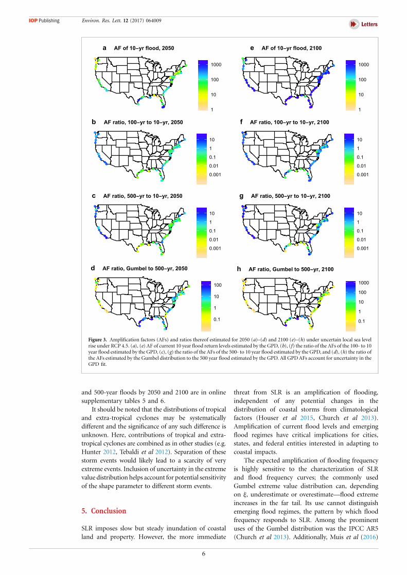
Figure 3 shows the expected amplification of thecurrent 10-year flood and its ratio to other flood levelsfor a set (N¼ 69) of long-duration tide gauges acrossUScoastlines under RCP 4.5, corresponding to a likelyglobal mean temperature increase of 2 °C–3.6 °C by2100 (Van Vuuren et al 2011). While the Gumbeldistributionunderestimates andoverestimates theAFofthe current 500-year flood by 1–2 orders of magnitude(figures 3(d) and (h)), the GPD captures distinct floodregimes—the heightened AF of more extreme floodingfor areas with negative j (and the opposite for areas withpositive j; figures 3(b), (c), (f) and (g)). AFs in figure 3are drastically different than those for the US in the AR5

15

5050

0

Seattle ( = 0.17)

AF

15

5050

0

San Francisco ( = 0.03)

AF

15

5050

0

New York ( = 0.19)

AF

15

5050

0

Charleston ( = 0.23)

AF

ξ

Expected AF10% 1% 0.2%

G GPD E[SLR] 10% 1% 0.2% Uncertain GPD

50 cm SLR Uncertain SLR

ξ

ξξ

G GPD E[SLR] 10% 1% 0.2% Uncertain GPD

50 cm SLR Uncertain SLR

G GPD E[SLR] 10% 1% 0.2% Uncertain GPD

50 cm SLR Uncertain SLR

G GPD E[SLR] 10% 1% 0.2% Uncertain GPD

50 cm SLR Uncertain SLR

Figure 2. Expected amplification factors (AFs) of different flood return levels (10% (�), 1% (△), and 0.2% (◊) annual chancefloods) for different extreme value distributions (GPD and Gumbel) and characterizations of sea level rise (SLR) for sites (Seattle, SanFrancisco, Charleston, and New York City) with varying shape parameters (negative, near-zero, and positive j). Amplificationscenarios include: (1) the Gumbel distribution with 0.5m deterministic SLR (column G), (2) the GPD with 0.5m deterministic SLRfor the 10-, 100-, and 500 years floods (GPD), (3) the GPD with expected SLR for 2050 under RCP 4.5 for the 10-, 100-, and 500-yearfloods (E[SLR]), (4–6) the GPD with uncertain SLR for 2050, integrated over the full probability distribution for SLR under RCP 4.5for the 10-, 100-, and 500-year floods (Uncertain SLR), and finally (7) the GPD with uncertain SLR for 2050, integrated over the fullprobability distribution for SLR under RCP 4.5 and accounting for uncertainty in the GPD fit (see Methods) for the 500-year flood(Uncertain GPD). With the Gumbel distribution, differences in the expected amplification of various flood levels with the sameamount of SLR are undetectable (�). The extreme value distribution (Gumbel vs. GPD) and use of only the expected level of SLR areresponsible for the largest degrees of error in flood frequencies with respect to SLR. Boxplots correspond to the 5th, 17th, 50th, 83rd,and 95th percentiles of the distribution of AFs. Median estimates of the shape factor are shown in the panel titles.

Environ. Res. Lett. 12 (2017) 064009

figure 13.25 (Church et al 2013), which used a Gumbeldistribution. With 50 cm of SLR, the AR5 under-estimates the AF of the 500-year flood in areas with anegative j andoverestimates it in areaswith positive j by1–3 orders of magnitude, respectively.

Under probabilistic relative sea level projectionsof Kopp et al (2014) for RCP 4.5 and whenaccounting for uncertainty in the GPD, we projecta median 25-fold increase (range of 1- to 914-fold) inthe expected annual number of local 100-year floodsfor tide-gauge locations along the contiguous UScoastline by 2050 (measured with respect todetrended sea level over the entire length of therecord; Buchanan et al 2016). These values jumpsignificantly by 2100 (median: 1729, range: 5–12546). As SLR gets to such high levels, lower floodlevels saturate first, yielding flooding influenced

5

primarily by tidal events rather than storm surges,and dampening the growth of the AF of all floodlevels along all coastlines (figures 3(e), (g) and (h)).This effect is also illustrated by the red curve in onlinesupplementary figure 1, demarcating flood levels in2100. Under RCP 8.5, a high greenhouse gasemissions pathway, a median 40-fold increase (range:1–1314) in the annual number of local 100 year floodsis expected by 2050 and a median 3467-fold increase(range: 5–16 829) by 2100. For illustrative purposes,the current 100-year flood in Seattle is expected tooccur 50.9 times a year, equal to an average of one100-year flood per week. The expected AFs of variousflood levels by 2050 and 2100 under RCP 4.5 and 8.5,accounting for uncertainty in the GPD fit, areprovided in online supplementary tables 1–2. Annualexpected flood frequencies of the 10-year, 100-year,

●●

●●●●●●●●●

●●●●●●●●●●●●

●●●

●●

●●●

●●●●

●●●●●●

●

●●

●●

●

●●●●

●●

●

●

1

10

100

1000

a AF of 10−yr flood, 2050

●●

●●●●●●●●●

●●●●●●●●●●●●

●●●●

●

●●●

●●●●

●●●●●●

●

●●

●●

●

●●●●

●●

●

●

0.001

0.01

0.1

1

10

b AF ratio, 100−yr to 10−yr, 2050

●●

●●●●●●●●●

●●●●●●●●●●●●

●●●●

●

●●●

●●●●

●●●●●●

●

●●

●●

●

●●●●

●●

●

●

0.001

0.01

0.1

1

10

c AF ratio, 500−yr to 10−yr, 2050

●●

●●●●●●●●●

●●●●●●●●●●●●

●●●

●●

●●●

●●●●

●●●●●●

●

●●

●●

●

●●●●

●●

●

●

0.1

1

10

100

d AF ratio, Gumbel to 500−yr, 2050

●●

●●●●●●●●●

●●●●●●●●●●●●

●●●

●●

●●●

●●●●

●●●●●●

●

●●

●●

●

●●●●

●●

●

●

1

10

100

1000

e AF of 10−yr flood, 2100

●●

●●●●●●●●●

●●●●●●●●●●●●

●●●●

●

●●●

●●●●

●●●●●●

●

●●

●●

●

●●●●

●●

●

●

0.001

0.01

0.1

1

10

f AF ratio, 100−yr to 10−yr, 2100

●●

●●●●●●●●●

●●●●●●●●●●●●

●●●●

●

●●●

●●●●

●●●●●●

●

●●

●●

●

●●●●

●●

●

●

0.001

0.01

0.1

1

10

g AF ratio, 500−yr to 10−yr, 2100

●●

●●●●●●●●●

●●●●●●●●●●●●

●●●

●●

●●●

●●●●

●●●●●●

●

●●

●●

●

●●●●

●●

●

●

0.1

1

10

100

1000

h AF ratio, Gumbel to 500−yr, 2100

Figure 3. Amplification factors (AFs) and ratios thereof estimated for 2050 (a)–(d) and 2100 (e)–(h) under uncertain local sea levelrise under RCP 4.5. (a), (e) AF of current 10 year flood return levels estimated by the GPD, (b), (f) the ratio of the AFs of the 100- to 10year flood estimated by the GPD, (c), (g) the ratio of the AFs of the 500- to 10 year flood estimated by the GPD, and (d), (h) the ratio ofthe AFs estimated by the Gumbel distribution to the 500 year flood estimated by the GPD. All GPDAFs account for uncertainty in theGPD fit.

Environ. Res. Lett. 12 (2017) 064009

and 500-year floods by 2050 and 2100 are in onlinesupplementary tables 5 and 6.

It should be noted that the distributions of tropicaland extra-tropical cyclones may be systematicallydifferent and the significance of any such difference isunknown. Here, contributions of tropical and extra-tropical cyclones are combined as in other studies (e.g.Hunter 2012, Tebaldi et al 2012). Separation of thesestorm events would likely lead to a scarcity of veryextreme events. Inclusion of uncertainty in the extremevalue distribution helps account for potential sensitivityof the shape parameter to different storm events.

5. Conclusion

SLR imposes slow but steady inundation of coastalland and property. However, the more immediate

6

threat from SLR is an amplification of flooding,independent of any potential changes in thedistribution of coastal storms from climatologicalfactors (Houser et al 2015, Church et al 2013).Amplification of current flood levels and emergingflood regimes have critical implications for cities,states, and federal entities interested in adapting tocoastal impacts.

The expected amplification of flooding frequencyis highly sensitive to the characterization of SLRand flood frequency curves; the commonly usedGumbel extreme value distribution can, dependingon j, underestimate or overestimate—flood extremeincreases in the far tail. Its use cannot distinguishemerging flood regimes, the pattern by which floodfrequency responds to SLR. Among the prominentuses of the Gumbel distribution was the IPCC AR5(Church et al 2013). Additionally, Muis et al (2016)

Environ. Res. Lett. 12 (2017) 064009

use the Gumbel distribution to derive a global data setof extreme sea levels; this data now populates theDynamic Interactive Vulnerability Analysis (DIVA)model, which is used extensively to assess impacts ofsea level rise (e.g. Hinkel et al 2014). The AR5amplification values may be seriously misleadingbecause using the Gumbel distribution implies thatamplification of flood frequency is invariant acrossflood levels. For example, this assumes that thefrequency of extreme events like a 500-year flood willincrease by the same magnitude as lesser extremes,potentially projecting overly catastrophic flood haz-ards in some areas while underestimating floodhazards elsewhere. Prominent use of the Gumbeldistribution in the IPCC—which has a specialinfluence on policy makers—and elsewhere creates arisk that policy makers will implement policy based onthe wrong information. While using a rule of thumb(implicit in the Gumbel distribution) is practical, itover-simplifies flood hazard characterization andcould result in costly misjudgments by planners. Thisis particularly important as coastal areas tend to beearly adopters of climate change adaptation planning(nearly 80% of US adaptation plans in a recent meta-analysis were in coastal states; Woodruff and Stults2016). The use of the GPD is therefore preferable forflood risk assessment of the emerging non-stationaryclimate.

Using the GPD, locations with positive j (like NewYork City, Baltimore, Washington DC, and Key West)can expect disproportionate amplification of higherfrequency events, whereas those with negative j (suchas Seattle, San Diego, and Los Angeles) can expect adisproportionate amplification of lower frequencyflooding. Effective policies should initially increaseresilience to historical flooding in areas with emergingflood regimes associated with positive j, and preparefor largely unprecedented flooding in areas withnegative j. Policies should also allow for adjustmentover time to address eventual flooding dominated bytidal events and permanent inundation (Sweet andPark 2014). Identification of areas with similar floodregimes by shape factor could facilitate the sharing ofadaptation strategies across coastal areas.

Acknowledgments

Support for this work was provided forMK B andMOby the National Science Foundation under Award EAR-1520683.We thankClaudia Tebaldi for her assistance indeveloping the extreme value distributions.

References

Buchanan M K, Kopp R E, Oppenheimer M and Tebaldi C 2016Allowances for evolving coastal flood risk under uncertainlocal sea-level rise Clim. Change 137 347–62

7

Church J A et al 2013 Chapter 13: sea level change ClimateChange 2013: The Physical Science Basis. Contribution ofWorking Group I to the Fifth Assessment Report of theIntergovernmental Panel on Climate Change ed T FStocker, D Qin, G K Plattner, M Tignor, S K Allen, JBoschung, A Nauels, Y Xia, V Bex and P Midgley(Cambridge University Press) pp 1137–1216 (https://doi.org/10.1017/CBO9781107415324.026)

Coles S, Bawa J, Trenner L and Dorazio P 2001 An Introductionto Statistical Modeling of Extreme Values (London:Springer)

DeConto R M and Pollard D 2016 Contribution of Antarctica topast and future sea-level rise Nature 531 591–7

Douglas E et al 2016 Climate change and sea level riseprojections for Boston: the Boston Research AdvisoryGroup Report Technical report (Boston, MA: ClimateReady Boston)

Gilleland E and Katz R W 2011 New software to analyze howextremes change over time Eos, Trans. Amer. Geophys.Union 92 13–20

Hinkel J, Lincke D, Vafeidis A T, Perrette M, Nicholls R J, TolR S, Marzeion B, Fettweis X, Ionescu C and LevermannA 2014 Coastal flood damage and adaptation costs under21st century sea-level rise Proc. Natl Acad. Sci. 1113292–7

Houser T, Hsiang S, Kopp R and Larsen K 2015 Economic Risksof Climate Change: An American Prospectus (New York:Columbia University Press)

Hsiang S M and Jina A S 2014 The causal effect ofenvironmental catastrophe on long-run economic growth:evidence from 6700 cyclones Technical report (NationalBureau of Economic Research)

Hunter J 2012 A simple technique for estimating an allowancefor uncertain sea-level rise Clim. Change 113 239–52

Jensen J L W V 1906 Sur les fonctions convexes et les inégalitésentre les valeurs moyennes Acta Math. 30 175–93

Knutson T R, McBride J L, Chan J, Emanuel K, Holland G,Landsea C, Held I, Kossin J P, Srivastava A and Sugi M2010 Tropical cyclones and climate change Nat. Geosci. 3157–63

Kopp R E, Horton R M, Little C M, Mitrovica J X,Oppenheimer M, Rasmussen D, Strauss B H and TebaldiC 2014 Probabilistic 21st and 22nd century sea-levelprojections at a global network of tide-gauge sites Earth’sFuture 2 383–406

Lin N, Emanuel K, Oppenheimer M and Vanmarcke E 2012Physically based assessment of hurricane surge threatunder climate change Nat. Clim. Change 2 462–7

Muis S, Verlaan M, Winsemius H C, Aerts J C and Ward P J2016 A global reanalysis of storm surges and extreme sealevels Nat. Commun. 7 11969

NERC 1975 Flood studies report Technical report (London:National Environment Research Council)

NYC 2013 A stronger, more resilient New York New York CityTechnical Report

Pugh D T 1996 Tides, Surges and Mean Sea-level (Reprinted withCorrections) (Hoboken, NJ: Wiley)

Sweet W V and Park J 2014 From the extreme to the mean:acceleration and tipping points of coastal inundation fromsea level rise Earth’s Future 2 579–600

Tebaldi C, Strauss B H and Zervas C E 2012 Modelling sea levelrise impacts on storm surges along US coasts Environ. Res.Lett. 7 014032

USACE 2015 North Atlantic coast comprehensive study: Resilientadaptation to increasing risk Technical report (US ArmyCorps of Engineers)

Van Vuuren D P et al 2011 The representative concentrationpathways: an overview Clim. Change 109 5–31

Woodruff S C and Stults M 2016 Numerous strategies butlimited implementation guidance in US local adaptationplans Nat. Clim. Change 6 796–802