amplifier figure of merit (fom)
TRANSCRIPT

11/14/2018
1
Analog Electronics(Course Code: EE314)
Lecture 33: Frequency Response contd..
Indian Institute of Technology Jodhpur, Year 2018
Course Instructor: Shree PrakashTiwari
Email: [email protected]
b h //h / /Webpage: http://home.iitj.ac.in/~sptiwari/
Course related documents will be uploaded on http://home.iitj.ac.in/~sptiwari/EE314/
1
Note: The information provided in the slides are taken form text books for microelectronics (including Sedra & Smith, B. Razavi), and various other resources from internet, for teaching/academic use only
Amplifier Figure of Merit (FOM)• The gain‐bandwidth product is commonly used to benchmark amplifiers. – We wish to maximize both the gain and the bandwidthWe wish to maximize both the gain and the bandwidth.
• Power consumption is also an important attribute.– We wish to minimize the power consumption.
CCC
LCCm
VI
CRRg
1
nConsumptioPower
BandwidthGain
LCCT
CCC
CVV
VI
1
nConsumptioPower
Operation at low T, low VCC, and with small CL superior FOM

11/14/2018
2
Bode Plot
• The transfer function of a circuit can be written in the general form
jj
• Rules for generating a Bode magnitude vs. frequency plot:
21
210
11
11
)(
pp
zz
jj
jj
AjH
A0 is the low-frequency gainzj are “zero” frequenciespj are “pole” frequencies
g g g q y p
– As passes each zero frequency, the slope of |H(j)| increasesby 20dB/dec.
– As passes each pole frequency, the slope of |H(j)| decreases by 20dB/dec.
Bode Plot Example
• This circuit has only one pole at ωp1=1/(RCCL); the slope of |Av|decreases from 0 to ‐20dB/dec at ωp1.
LCp CR
11
• In general, if node j in the signal path has a small‐signal resistance of Rj to ground and a capacitance Cj to ground, then it contributes a pole at frequency (RjCj)
‐1

11/14/2018
3
• The impedance of CL decreases at high frequencies, so that it shunts some of the output current to ground.
Av Roll‐Off due to CL
0LD
p CR
10
LDmv Cj
RgA1
||
Pole Identification Example 1
0
inGp CR
11
LDp CR
12

11/14/2018
4
Pole Identification Example 2
0 0
inm
G
p
Cg
R
1||
11
LDp CR
12
Pole Identification Example 3
inSp CR
11
LCp CR
12

11/14/2018
5
High‐Frequency BJT Model
• The BJT inherently has junction capacitances which affect its performance at high frequencies.Collector junction depletion capacitance CCollector junction: depletion capacitance, CEmitter junction: depletion capacitance, Cje, and also
diffusion capacitance, Cb.
jeb CCC
BJT High‐Frequency Model (cont’d)
• In an integrated circuit, the BJTs are fabricated in the surface region of a Si wafer substrate; another junction exists between the collector and substratejunction exists between the collector and substrate, resulting in substrate junction capacitance, CCS.
BJT cross-section BJT small-signal model

11/14/2018
6
Example: BJT Capacitances• The various junction capacitances within each BJT are explicitly shown in the circuit diagram on the right.
MOSFET Intrinsic Capacitances
The MOSFET has intrinsic capacitances which affect its performance at high frequencies:1. gate oxide capacitance between the gate and channel,1. gate oxide capacitance between the gate and channel,2. overlap and fringing capacitances between the gate and the
source/drain regions, and3. source‐bulk & drain‐bulk junction capacitances (CSB & CDB).

11/14/2018
7
High‐Frequency MOSFET Model
• The gate oxide capacitance can be decomposed into a capacitance between the gate and the source (C1) and a capacitance between the gate and the drain (C )a capacitance between the gate and the drain (C2). – In saturation, C1 (2/3)×Cgate, and C2 0.
– C1 in parallel with the source overlap/fringing capacitance CGS– C2 in parallel with the drain overlap/fringing capacitance CGD
Example
CS stage
…with MOSFET capacitancesexplicitly shown
Simplified circuit for high‐frequency analysis

11/14/2018
8
Transit Frequency, fT• The “transit” or “cut‐off” frequency, fT, is a measure of the intrinsic speed of a transistor, and is defined as the frequency where the current gain falls to 1the frequency where the current gain falls to 1.
Conceptual set-up to measure fT
i
inin Z
VI
inmout VgI
mT
inTminm
in
out
g
CjgZg
I
I
1
1
C
gf mT 2
inZin
T C
Transit Frequency, fT• The “transit” or “cut‐off” frequency, fT, is a measure of the intrinsic speed of a transistor, and is defined as the frequency where the current gain falls to 1the frequency where the current gain falls to 1.
Conceptual set‐up to measure fT
mT
inTminm
in
out
g
CjgZg
I
I
1
1
i
inin Z
VI
inmout VgI
GS
mT C
gf 2
inT CinZ

11/14/2018
9
Dealing with a Floating Capacitance
• Recall that a pole is computed by finding the resistance and capacitance between a node and (AC) GROUND.
• It is not straightforward to compute the pole due to C1in the circuit below, because neither of its terminals is grounded.
Dealing with a Floating Capacitance
• Recall that a pole is computed by finding the resistance and capacitance between a node and (AC) GROUND.
• It is not straightforward to compute the pole due to CFin the circuit below, because neither of its terminals is grounded.
11/14/2018
10
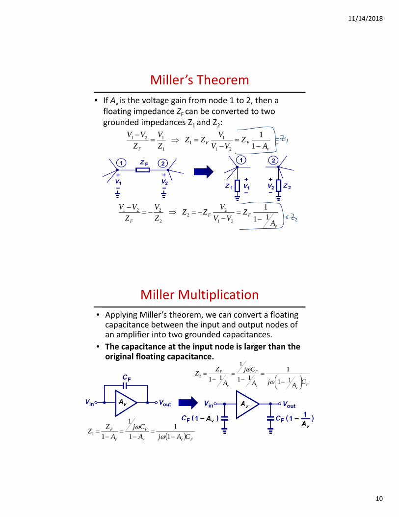
Miller’s Theorem
• If Av is the voltage gain from node 1 to 2, then a floating impedance ZF can be converted to two grounded impedances Z and Z :grounded impedances Z1 and Z2:
vFF
F AZ
VV
VZZ
Z
V
Z
VV
1
1
21
11
1
121
v
FFF A
ZVV
VZZ
Z
V
Z
VV11
1
21
22
2
221
Miller Multiplication
• Applying Miller’s theorem, we can convert a floating capacitance between the input and output nodes of an amplifier into two grounded capacitances.an amplifier into two grounded capacitances.
• The capacitance at the input node is larger than the original floating capacitance.
Fv
v
F
v
F
CAjA
Cj
A
ZZ
11
111
1
112
Fvv
F
v
F
CAjA
Cj
A
ZZ
1
1
1
1
11

11/14/2018
11
Miller Multiplication
• Applying Miller’s theorem, we can convert a floating capacitance between the input and output nodes of an amplifier into two grounded capacitances.an amplifier into two grounded capacitances.
• The capacitance at the input node is larger than the original floating capacitance.
vAA 0
F
F
v
F
CAjA
Cj
A
ZZ
00
211
111
1
11
F
F
v
F
CAjA
Cj
A
ZZ
001 1
1
1
1
1
Application of Miller’s Theorem
inp CRgR
1
1, FCmS
p CRgR 1
FCm
C
outp
CRg
R
1
1
1,

11/14/2018
12
Application of Miller’s Theorem
0
1 1
FDmGin CRgR
1
1F
DmD
out
CRg
R
1
1
1
Small‐Signal Model for CE Stage

11/14/2018
13
Next
• Algebra of Sinusoidal and Bode Plots
• Ac analysis contd..