Saclay-t19/013

Amplitudes’ Positivity, Weak Gravity Conjecture, and Modified Gravity

Brando Bellazzini,1 Matthew Lewandowski,1 and Javi Serra2

1Institut de Physique Theorique, Universite Paris Saclay, CEA, CNRS, F-91191 Gif-sur-Yvette, France2Physik-Department, Technische Universitat Munchen, 85748 Garching, Germany

We derive new positivity bounds for scattering amplitudes in theories with a massless gravitonin the spectrum in four spacetime dimensions, of relevance for the weak gravity conjecture andmodified gravity theories. The bounds imply that extremal black holes are self-repulsive, M/|Q| < 1in suitable units, and that they are unstable to decay to smaller extremal black holes, providing anS-matrix proof of the weak gravity conjecture. We also present other applications of our bounds tothe effective field theory of axions, P (X) theories, weakly broken galileons, and curved spacetimes.

I. INTRODUCTION

The general properties of the S-matrix, unitarity, an-alyticity and crossing symmetry, imply dispersion rela-tions for forward elastic scattering amplitudes, which inturn yield positivity bounds for amplitudes evaluated inthe infrared (IR). They provide therefore non-trivial con-straints on the coefficients of operators in the effectivefield theories (EFTs) that are used to calculate the am-plitudes at low energy [1, 2]. An EFT with operatorsentering the action with the “wrong” sign cannot ariseas the low-energy limit of a consistent ultraviolet (UV)theory satisfying the S-matrix axioms, and thus lives inthe “swampland.” The proof of the a-theorem [3, 4] isperhaps the prime example of an application of thesepositivity bounds.

In this paper, new amplitudes’ positivities are derivedfor theories with a massless graviton in the spectrum,despite the fact that the forward elastic 2-to-2 scatteringis singular (Coulomb singularity). These new positivitybounds, and the way we circumvent the graviton forwardsingularity, are extremely important because they allowus to address the swampland program of quantum grav-ity and modified gravity theories, providing general androbust results.

As a notable application, we study the Einstein-Maxwell theory, i.e. the low-energy EFT of an abelianU(1) gauge theory coupled to gravity, and show that ourpositivity bounds imply certain inequalities among theleading higher-dimensional operators affecting the blackhole’s extremality condition (the minimal mass for whicha charged black hole can exist, as opposed to a naked sin-gularity). We show that extremal black holes of mass M

and U(1)-charge Q must satisfy√

2mPl|Q|/M > 1, sothat they are self-repulsive and are no longer kinemati-cally forbidden from decaying into smaller extremal blackholes. Moreover, these positivity bounds provide a proofof the mild form of the weak gravity conjecture (WGC)[5]: extremal black holes are themselves charged statesin the theory for which gravity is the weakest force.

Another interesting application is for shift-symmetric

scalars such as in the EFT of axions, P (X) theories, andweakly broken galileons. The latter are found to have atiny cutoff if they are to originate from a canonical micro-scopic S-matrix, ΛUV < few× (H3mPl)

1/4 ∼ 1/(107km),i.e. orders of magnitude smaller than the strong couplingscale Λ3 = (H2mPl)

1/3 ∼ 1/(103 km).Finally, we also discuss how our methods allow us to

derive positivity bounds in a mildly curved de Sitter (dS)spacetime.

II. REGULATING THE FORWARD LIMIT

The forward elastic amplitude of massless particles ofpolarizations labelled by zi is dominated by the universalCoulomb singularity

Mz1z2(s, t→ 0) = − s2

m2Plt

+O(s) , (1)

because of the equivalence principle or, equivalently, be-cause of factorization of the amplitude at the pole intothe soft emission of an on-shell massless graviton, whichhas universal strength given by the reduced Planck massmPl. Since the coefficient of s2 in (1) would enter the dis-persion relation in the forward limit for particles of anyspin zi [2], see (4), the naıve application of the Cauchy in-tegral theorem to Mz1z2(s, t→ 0) yields ∞ =∞, whichis consistent, but admittedly not very informative. Itis clear, however, that this divergence is due to long-distance physics, i.e. vanishing exchanged momentum,corresponding to the graviton probing arbitrarily largemacroscopic distances even for large center-of-mass en-ergy squared s. In any EFT the presumption is thatthe IR physics is known, therefore one should be ableto track and resolve the source of the forward singular-ity. Indeed, we show below how to massage the dis-persion relation into an effective, regulated expression∞ − ∞ = finite > 0, returning something meaningful,free of ambiguity and in fact of a definite sign, whichcan be used for charting the swampland in gravitationaltheories.

arX

iv:1

902.

0325

0v4

[he

p-th

] 1

7 Se

p 20

19

2

The key observation is that the Coulomb singularityis due to the infinite flat-space volume. One would betempted to regulate it by putting the system in a box(or perhaps in anti-de Sitter), however that would breakLorentz invariance and spoil the usual arguments thatlead to positivity bounds. A compromise is enough forour purposes: we regulate the system by putting it ona cylinder. That is, we compactify one spatial directionon a circle of length L, while the other three spacetimedimensions remain flat and infinite. In this way we canuse 3D Lorentz invariance of the non-compact dimensionsand scatter 3D asymptotic states, while at the same timegetting rid of the Coulomb singularity. Indeed, there isno propagating massless graviton in D = 3, hence nos2/t-term for any finite value of L.1 The 4D gravitonhas not fully disappeared though, it has rather left threepropagating avatars (on top of a non-propagating auxil-iary field gµν which gives rise to contact terms):

gMN → {σ , Vµ , KK-modes} , (2)

a massless dilaton σ, a massless (abelian) graviphotonVµ, and an infinite tower of Kaluza-Klein (KK) modeswith masses m2

n ∼ n2/L2. In the limit L → ∞, that wetake at the end after isolating the diverging terms, onerecovers the 4D dynamics we are interested in.2

There is another advantage of compactifying to D = 3,namely that asymptotic states all behave as masslessscalars at high energies because the massless 3D little-group is trivial. This explains why the massless gravipho-ton is dual to a scalar field, and also explains why a mas-sive KK-graviton decomposes into a massless scalar, amassless vector (dual to a massless scalar again) and anon-dynamical 2-tensor at high energy.

In the following (see Sec. III) we will be interested inscattering non-gravitational massless states, for examplethe 3D photon Aµ and the 3D scalar Φ that live inside the

4D photon AM , in the 4D Einstein-Maxwell theory re-duced to 3D. Since there is no 3D massless graviton and

1 The tree-level exchange of a 3D auxiliary 2-tensor gµν does giverise to an s2/t-term. However, since the associated singularitydoes not correspond to any physical particle, i.e. there is no phys-ical graviton in D = 3, higher-order corrections actually removeit. In App. A we show that the 3D Einstein-Hilbert amplitude isindeed regular in the forward limit (in fact constant), thereforeirrelevant and can be subtracted in the dispersion relation (4).This should be contrasted to the D = 4 case, where no correctioncan erase the t-channel pole.

2 We stress that we are not discussing 3D toy models as done in asimilar context in [6, 7]. Those references work in a truly D = 3setup, since in the IR spectrum there are neither the masslessdilaton and the massless graviphoton, nor the massless 3D scalarΦ inside the 4D photon AM (see Sec. III), nor the tower of mas-sive (but light) KK modes, all of which are needed to correctlyreproduce the 4D dynamics and thus affect the positivity bounds.Incidentally, the conclusion about the connection between neu-trinos and electrons pointed out in [7] seems premature, since the3D IR spectrum of the compactification of the Standard Modelis very different, in particular neutral light states other than neu-trinos are abundant, and have non-minimal couplings.

the states are either gaped, non-propagating, or equiv-alent to simple scalars, we require a 3D Froissart-likebound

lims→∞

|Mz1z2(s, t = 0)/s2| → 0 , zi = Φ , A , (3)

where with a slight abuse of notation we are using zi tolabel now the scattered 3D states. This is just the sameassumption of polynomial boundedness that one acceptsin 4D to derive dispersion relations and positivity boundsfor the coefficient of e.g. (∂π)4 or (FµνF

µν)2, when 4Dgravity is neglected or non-dynamical [1].3

For a gapped system, the Froissart bound becomes anactual theorem [8, 9], providing the asymptotic bound

|M(s→∞)| < const · s logD−2 s for D ≥ 3 [10, 11]. Onecould thus even argue that (3) is automatically satisfiedby giving a mass to the dilaton and to the graviphoton,then deriving the bound, and finally taking the masslesslimit, which is smooth for either field due to the abeliannature of the graviphoton. We will not commit to thisview and content ourselves with assuming (3) and ex-tracting the corresponding implications.

Therefore, under exactly the usual assumptions thatlead to the familiar positivity bounds for systems of spin-0 and spin-1 massless particles in 4D, and repeating simi-lar steps to those outlined in for example [2], we obtain a(provisional) dispersion relation for our IR-regulated 4Dgravitational theory

az1z2 =2

π

∫ ∞

0

ds

s3ImMz1z2(s, t = 0) > 0 , (4)

where the low-energy scattering amplitude for the 3Dstates zi is now regular in the forward elastic limit

Mz1z2(s, t→ 0) = az1z2s2 + . . . . (5)

The dimensional reduction to 3D has left a univer-sal contribution from gravitational zero and KK modes.Each KK mode gives

az1z2KK ∝1

L2m4PlmKK

∝ 1

Lm4Pl|n|

, (6)

where we used that the nth KK-mode mass is mKK ∝|n|π/L. While each such contribution is subleading withrespect to the terms we want to bound in the follow-ing sections, their sum is actually logarithmically diver-gent. In addition, zero-mode loops generate s3/2-termsin the amplitude, which dominate over the s2-terms atlow energy, seemingly swamping again the information

3 In App. B we discuss how our conclusions adapt to relaxing theFroissart bound (3). We show in particular that an asymptoticform of the WGC, i.e. for very large extremal black holes, canstill be proven even assuming no Froissart-like bound. In thiscontext, we also discuss amplitudes’ positivity for gravitationalstates, such as the 3D dilaton.

3

about az1z2 . In fact, these problems can be easily solvedbecause the right-hand side of the dispersion relation(4) reproduces the same growth, so that these other-wise large terms cancel out between the two sides of (4).Indeed, since the integrand itself in (4) is positive bythe optical theorem, schematically ImMz1z2(s, t = 0) =∑x |Mz1z2→x|2× (phase space), we can move to the left-

hand side any contribution from intermediate states x in|Mz1z2→x|2 and still get a positivity bound due to theremaining set of intermediate states. Specifically, we canmove to the left-hand side the contributions from the in-termediate IR states, such as the KK modes or anythingthat is calculable within the EFT (e.g. IR loops, that is,the light multi-particle intermediate states). The zero-and KK-mode contributions get subtracted and one isleft to calculate just the contact terms suppressed by thecutoff ΛUV , that is, those that are generated by integrat-ing out genuine UV states.

Just to illustrate this general point with a simple tree-level example, let us consider ΦΦ → ΦΦ scattering withthe exchange of a scalar state S coupled to (∂Φ)2,

MΦΦS (s, t) = − 2c

m2PlL

(s2

s−m2S + iε

+ crossing

), (7)

where c is a fixed O(1) number. This contributes to az1z2

in (5) by an amount aΦΦS = 4c/(m2

PlLm2S). The imagi-

nary part (associated to the production of S) is

ImMΦΦS (s, t = 0) =

2πc

m2PlL

m4Sδ(s−m2

S) + . . . , (8)

precisely such that

aΦΦS − 2

π

∫ ∞

0

ds

s3ImMΦΦ

S (s, t = 0) = 0 , (9)

as expected on general grounds.The KK-mode contributions to az1z2 in (6) actually

arise at one loop, but the reasoning based on the opti-cal theorem is completely general and works as in theprevious example. This can be understood by discretiz-ing the KK branch cut in a series of poles. Likewise forthe contribution of the zero modes.4. The concrete de-tails of how these contributions are subtracted are givenin App. C. Here we only note that the KK modes, whichgrow the “extra” dimension as seen from a low-energy 3Dobserver, reproduce nicely the 4D universal gravitationalcontribution to the RG running of az1z2 . This contribu-tion is positive and as noted above would dominate theleft-hand side of (4). Since we can subtract it, whichamounts to setting the renormalization scale at which

4 The tree-level exchange of an exactly massless dilaton is incon-sequential because s+ t+ u = const. If a stabilisation potentialfor the dilaton σ is included, for example a mass term ∼ σ2/L2,the tree-level subtraction also works for the dilaton pole.

az1z2 is evaluated at the cutoff where UV and IR ampli-tudes are matched, our final dispersion relation properlycaptures the UV physics we are interested in.

All in all, our provisional dispersion relation (4) is re-arranged into a much more informative expression

az1z2−az1z2KK,IR =2

π

∫ ∞

0

ds

s3ImMz1z2(s, t = 0) > 0 , (10)

where M is the amplitude with the aforementioned grav-itational zero- and KK-mode loop contributions sub-tracted. The left-hand side is therefore obtained by tak-ing into account only the s2-contributions to the elas-tic z1z2-scattering due to the tree-level interactions withmassless particles such as the graviphoton and the dila-ton, as well as the UV generated contact terms, especiallythose from the auxiliary field gµν .5 The two sides (factorL−1) of the subtracted dispersion relation (10), are notonly finite for L→∞, but they are also positive becauseof the optical theorem. We note that removing the IRmodes from the positivity bound is always possible butis useful in practice only for UV completions that arenot strongly coupled at ΛUV , because it would becomemurky to assign what is IR (KK) and what is UV physicsat around the scale ΛUV . The subtracted dispersion re-lation is instead sharp and useful for weakly coupled UVcompletions.

One general lesson is that gravity still has a finite ef-fect on the positivity bounds even after removing theCoulomb singularity, due to the dilaton, the gravipho-ton, and the auxiliary 2-tensor. This will be reflected inthe new bounds derived for the explicit examples that wediscuss next.

III. EINSTEIN-MAXWELL EFT

In this section we focus on the important example ofthe Einstein-Maxwell EFT, whose leading 4D operatorsare

S =

∫d4x√|g|[m2

Pl

2R− 1

4FMN FMN (11)

+α1

4m4Pl

(FMN FMN

)2

+α2

4m4Pl

(ˆFMN FMN

)2

+α3

2m2Pl

FABFCDWABCD

],

where WABCD is the Weyl tensor andˆFMN =

εMNABFAB/2. The dependence on the UV scale ΛUV

that generates the αi is absorbed into their definitions.

5 Incidentally, the resulting contact terms can not be subtractedexcept for obtaining the useless relation 0 = 0, since they do notcorrespond to any IR intermediate state that alone would satisfy(3).

4

These are the most general (parity preserving) four-derivative operators, up to field redefinitions [6, 12]. Inorder to regulate the 4D forward limit and apply thepositivity bounds (10), we compactify the z direction asdescribed in the previous section

ds24[gMN ] = eσds2

3[gµν ] + e−σ (dz + Vµdxµ)

2, (12)

AMdxM = Aµdx

µ + Φ dz , (13)

where all of the 3D fields are functions only of (t, x, y).Focusing on terms which contribute to the s2 part of theamplitude for ΦΦ → ΦΦ, AA → AA, and ΦA → ΦAonly, the terms in the action that we must retain are

S = L

∫d3x√−g

{m2

Pl

2

(R− 1

2(∂σ)2 − 1

4V µνVµν

)

− 1

4(1− σ)FµνFµν − (1 + σ)

1

2(∂Φ)2 − 1

2FµνV

µνΦ

+α1

4m4Pl

(FµνFµν + 2(∂Φ)2

)2+

α2

m4Pl

(εµνρFµν∂ρΦ)2

+α3

m2Pl

[FρµFρν − ∂µΦ∂νΦ]

(Rµν − 1

3gµνR

+1

3gµν�σ −∇µ∇νσ

)

− α3

m2Pl

Fµν∂ρΦ (∇ρV µν + gµρ∇αV να)

}, (14)

where we made a field redefinition Aµ → Aµ + ΦVµ tomake gauge invariance manifest. The gµν propagates nodegrees of freedom in D = 3 and we can integrate itout, which is effectively equivalent to plugging the lowest-order equations of motion Rµν − 1

2gµνR = Tµν/(Lm2

Pl)into the interaction terms, generating new contact terms.After removing �σ from the interactions with anotherfield redefinition we get

S = L

∫d3x√−g

{m2

Pl

2

(R− 1

2(∂σ)2 − 1

4V 2

)

− 1

4(1− σ)F 2 − 1

2(1 + σ)(∂Φ)2 − 1

2FµνV

µνΦ (15)

+α1

4m4Pl

(F 2 + 2(∂Φ)2

)2+

α2

m4Pl

(εµνρFµν∂ρΦ)2

+α3

m4Pl

[FρµF

ρνFµσFνσ −1

2F 4 − (∂Φ)4 +

1

2F 2(∂Φ)2

]

− α3

m2Pl

(FρµFρν − ∂µΦ∂νΦ)∇µ∇νσ

− α3

m2Pl

Fµν∂ρΦ (∇ρV µν + gµρ∇αV να)

},

-0.4 -0.2 0.0 0.2 0.4-1.0

-0.5

0.0

0.5

1.0

Α1

Α3

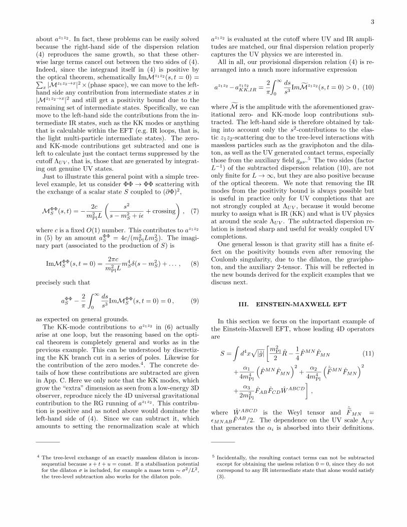
FIG. 1. Positivity bounds (19, 20) require α1 and α3 to liveinside the the smaller green wedge. The blue striped re-gion is where extremal black holes are self-repulsive, |Q| >M/(

√2mPl).

where F 2 = FµνFµν , and the same for V . The associated

subtracted forward elastic scattering amplitudes are

M(ΦΦ→ ΦΦ)(s, t = 0) =2s2

m4PlL

(2α1 − α3) > 0 , (16)

M(AA→ AA)(s, t = 0) =2s2

m4PlL

(2α1 + α3) > 0 , (17)

M(ΦA→ ΦA)(s, t = 0) =4s2

m4PlL

α2 > 0 . (18)

Therefore, the associated positivity bounds read

2α1 − α3 > 0 , (19)

2α1 + α3 > 0 , (20)

α2 > 0 , (21)

or, equivalently, α1 > |α3|/2, α2 > 0. These new pos-itivity bounds are one of the main results of this pa-per. In Fig. 1 we show the region constrained in the(α1, α3)-plane, which provides non-trivial constraints onthe 4D coefficients of the EFT (11) that includes a mass-less graviton in the spectrum.

Remarkably, these bounds are stronger, meaning moregeneral, than just pure 4D Euler-Heisenberg EFT with-out gravity [1, 2, 13], and carry extra information aboutα3, which enters the black hole extremality condition aswe discuss in Sec. IV.

Moreover, our homogeneous bounds (19 – 21) are dis-tinct from the order-of-magnitude causality bounds onO(|α3|) [13, 14], which are derived assuming positivity oftime delay and tree-level UV completion of the Einstein-Maxwell lagrangian. See also [14, 15] for a nice discus-sion of detectability of superluminal propagation withinan EFT, and how the Euler-Heisenberg lagrangian limitof the real-world QED avoids superluminality [16].

It is interesting to compare the bounds (19 – 21) withthe 4D calculation of the same processes retaining the

5

Coulomb singularity in the t→ 0 limit

M↓↓4D =− s2

m2Plt− s

m2Pl

+2s2 (2α1 − α3)

m4Pl

, (22)

M↑↑4D =− s2

m2Plt− s

m2Pl

+2s2 (2α1 + α3)

m4Pl

, (23)

M↑↓4D = − s2

m2Plt− s

m2Pl

+4s2α2

m4Pl

, (24)

where the up and down arrows represent the two choicesof real linear polarizations.6 The lesson is that our 4D-regulated calculation, which works with 3D Lorentz in-variance of the cylinder, teaches us which finite partswe are allowed to retain for the positivity bounds: throwaway the s2/t singularity, the finite O(s) term, but retainprecisely the O(s2) term.

This immediately prompts us to expect a continuousset of positivity bounds associated with arbitrary linearpolarizations |c1,2〉 = (cθ1,2 | ↑1,2〉+ sθ1,2 | ↓1,2〉), namely

α3(c2θ1 + c2θ2) + 4α1c2θ1+θ2 + 4α2s

2θ1+θ2 > 0 , (25)

where cθ = cos θ and sθ = sin θ. We will check thebounds (25) from arbitrary linear combinations with ourcontrolled, IR-regulated method in future work.

IV. WEAK GRAVITY CONJECTURE ANDEXTREMAL BLACK HOLES

The leading higher-dimensional corrections αi in the4D Einstein-Maxwell EFT (11) modify the black holeextremality condition to [18]

( √2|Q|

M/mPl

)

extr.

= 1 +4

5

(4π)2m2Pl

M2(2α1 − α3) > 1 , (26)

where M is the black hole mass and Q its charge (in-cluding the gauge coupling), and we work around M 'QmPl

√2. Remarkably, on the right-hand side of this

expression one finds the same combination 2α1 − α3

bounded to be positive by (19). Therefore, positivitybounds imply a greater charge-to-mass ratio for extremalblack holes than in pure general relativity coupled min-imally to an abelian U(1) gauge theory. The lighter theextremal black hole, the larger the charge-to-mass ratio.Extremal black holes within the validity of the 4D EFT,i.e. whose Schwarzschild radius rs = M/4πm2

Pl is largerthan 1/ΛUV , are therefore self-repulsive.

The positivity bound (19) implies the mild form of theWGC [5], which states that a consistent theory of quan-tum gravity must contain massive charged states in the

6 We use real linear polarizations because they correspond to cross-ing symmetric amplitudes [2, 17], up to the terms due to theCoulomb singularity.

spectrum with |q| > m/(√

2mPl): the extremal blackholes of (26) are such states. As a result, the paradoxof stable extremal black holes has evaporated, since ex-tremal black holes are no longer kinematically forbid-den to decay into smaller black holes. Indeed, an ex-tremal black hole of mass M and charge Q cannot de-cay into states that all have larger mass-to-charge ra-tio, since the spectrum of masses and charges (mi, qi)is constrained by M >

∑imi and Q =

∑i qi, whereas∑

imi =∑i |qi|mi/|qi| > M which would be a contradic-

tion. This argument is evaded precisely by decay prod-ucts that contain one smaller extremal black hole, whichhas smaller mass-to-charge ratio (26) because of the pos-itivity bound (19).

Since the same combination of EFT coefficients,2α1 − α3, enters the Wald entropy shift [12, 13], ourpositivity bound (19) implies a larger black hole entropyas well.7 Notice, however, that the reverse is not true.Requiring that the shift of the Wald entropy (of electri-cally charged black holes) is positive as a starting point[12] does not produce the same bounds on α1 and α3, andsays nothing about α2; while (19) is reproduced by de-manding a positive entropy shift [12, 13], the conditions(20) 2α1 + α3 > 0, (21) α2 > 0, and (25) are not.

V. BOUNDS ON SCALARS

Our IR-regulated positivity bounds can now be usedto constrain scalar theories, e.g. the EFT of axions ormodified gravity theories, that have a massless gravitonin the spectrum.8 Let us consider for instance

L = −1

2(∂φ)2 +

a

4f4(∂φ)4 + . . . . (27)

Without gravity, the positivity bounds would imply a > 0[1], and one could expect the same bound to hold as longas f � mPl. However, what about the case f � mPl? Infact, even for the case f � mPl, things are not completelyobvious in modified gravity theories.

For example, in the cosmological context a P (X) the-ory is usually considered with a decay constant f nottoo far from

√mPlH ≡ Λ2 � mPl, where H is the Hub-

ble constant. However, the limit t → 0 is an IR limitwhere the exchanged momentum goes to zero, so thatintermediate massless particles such as the graviton af-fect macroscopic distances.9 Even if one regulates theIR limit with the largest scale in the problem and takest ∼ H2, the graviton Coulomb singularity (1) would

7 Positivity bounds of even higher-derivative terms [17] imply pos-itive shift in the Kerr black hole entropy, too [19].

8 Positivity bounds applied to the Lorentz invariant EFT of mas-sive gravity had a dramatic impact [20].

9 Incidentally, this is why we believe the assumptions in [21] arenot fully justified, since the graviton is probing curved spacetimeregions even at large s.

6

give a contribution to the forward scattering which isat least as large as the one that we want to retain,i.e. O(s2/m2

PlH2) = O(s2/f4), thus spoiling the argu-

ment that leads to a > 0. The same issue was orig-inally pointed out in the context of 4D massive grav-ity [20], where the intermediate transverse graviton com-petes with the galileon modes for the contribution to theaππ ∼ m2

g/Λ63 ∼ 1/(m2

PlH2) for a graviton mass mg ∼ H.

In the case of 4D massless gravity studied in this pa-per, after compactifying to D = 3 there is no Coulombsingularity, while even if the series of gravitational KKmodes (6) is formally logarithmically divergent, it can ac-tually be removed in the subtracted dispersion relation(10). The left-hand side of (10) is thus finite and domi-nated by the contact terms, and since neither the dilatonnor the graviphoton contribute at leading order to thes2-term in the forward φφ→ φφ scattering, we concludethat in fact

a > 0 (28)

holds true in any weakly coupled UV completion of anEFT of the type (27), such as P (X) theories coupled togravity, and in fact even for axions with f � mPl shouldtheir cutoff ΛUV = g∗f be smaller than the Planck mass.

More interesting conclusions apply to weakly brokengalileons [22, 23]. Let us consider for example

L = −1

2(∂π)2 − 1

2Λ33

(∂π)2�π +1

4Λ42

(∂π)4 + . . . , (29)

where one can imagine the natural situation where Λ2 �Λ3 since (∂π)4 weakly breaks the Galilean symmetrywhereas (∂π)2�π is an invariant. It was shown indeedthat the hierarchy

Λ42 ' H2m2

Pl , Λ33 ' H2mPl , (30)

is stable under the loop corrections due to gravity thatbreak the galileon symmetry [23], and in fact even largervalues of Λ2 such as (Hm2

Pl)1/3 are in principle consistent.

However, as estimated in [2, 24] and calculated in de-tail in [20], the scales Λ2 and Λ3 cannot be arbitrarilyseparated while keeping the cutoff ΛUV fixed in a theorywithout gravity, because the integrand under the disper-sion relations (4) is strictly positive and it gives the fol-lowing beyond positivity bound [20]:

aππ =1

Λ42

>2

π

∫ Λ2UV ds

s3ImMππ(s) ∝ 1

16π2

Λ8UV

Λ123

. (31)

We can now see that a similar bound survives even whenthe graviton is dynamical if the UV completion is as-sumed to be weakly coupled (at least up to Λ2). Fol-lowing the arguments of the previous sections, we cansubtract the gravitational KK modes after the 3D com-pactification, and then extract the following bound

1

Λ42L

>2

π

∫ Λ2UV ds

s3ImMππ(s) >

c

16π2

Λ8UV

LΛ123

, (32)

where in the last inequality we used the optical the-orem and retained the contribution to the inelas-tic cross-section into two galileon KK modes πk,∑k,mk<ΛUV

σ(ππ → πkπk). The constant c = O(10−4)is an inessential numerical factor resulting from integrat-ing over the phase space and then along the branch cut.Loop corrections to the s2-coefficient on the left-handside of the dispersion relation are either very small orhave been subtracted. The bound (32) nicely reproducesthe scaling from the calculation without gravity in (31).As a consequence, the hierarchy (30) between Λ2 and Λ3,which is stable because of symmetries, in fact requires anextremely small cutoff

ΛUV <(H3mPl

)1/4(

16π2

c

)1/8

∼ 1

107 km(33)

in order to be consistent with the beyond positivitybound (32) that applies in a gravity theory. Vainshteinscreening [25] is no longer a valid EFT argument at scalesshorter than Λ−1

UV [2, 26] because operators with arbi-trarily more derivatives per field insertion become large,non-suprisingly, since new degrees of freedom are excitedat ΛUV .

It would be interesting to apply these new and pow-erful beyond positivity bounds to other general and stillstructurally robust EFTs of modified gravity [27].

VI. CURVED SPACETIME

In this section we argue how positivity bounds can beextended to the case of spacetimes which are barely dS4

(or AdS4), as appears to be the case in our universe witha 4D cosmological constant Λ4 that is very close to thescale of the neutrino masses. One trivial way would be toassume that we can vary Λ4 down to zero while the EFTcoefficients we are interested in depending very little onsuch a change. We entertain instead another possibility,where Λ4 is held fixed and less relevant or even marginaloperators (e.g. Yukawa couplings) are varied.

It was shown in [28] that the Standard Model cou-pled to gravity has a landscape of 3D vacua which isaccessible by varying the properties of neutrinos (or thevalue of Λ4, or both) by just O(1). One could for ex-ample vary the mass of the lightest neutrino, or thetype (Dirac vs Majorana), or the mass splitting squared∆m2

12, etc.. As these parameters are varied one getsdS3 or AdS3 solutions (times the compact dimension)which are energetically favored over dS4. Importantly, aflat 3D Minkowski solution (times the compact dimen-sion) can be energetically favorable as well. This can bereached for example by varying ∆m2

12 from 8 · 10−5 eV2

to 1.5 · 10−5 eV2 for Majorana neutrinos [28]. Tuningthe theory with such a value, we can run again the posi-tivity arguments derived in the previous sections to con-strain the coefficients a of, say, a e4(Fµν)4/Λ4

UV , whichis obtained by integrating out massive charged states at

7

the UV scale ΛUV . Since the neutrinos are neutral andweakly coupled, one natural expectation is that chang-ing e.g. ∆m2

12 while holding everything else fixed, willnot dramatically backreact on the value of a, that isa(∆m2

12) = a(∆m212|SM ) + O(δ∆m2

12/ΛUV )2. Alterna-tively, if the see-saw scale Λν for generating Majorananeutrino masses, mν ∼ v2/Λν , is much higher than thescale ΛUV we are interested in, then the contributionfrom particles at Λν to the parameter a is quickly over-run by the physics at ΛUV . One would thus conclude thata > 0 even in dS4 with a finite Λ4, within an accuracyO(δ∆m2

12/Λ2UV ,Λ

4UV /Λ

4ν).

The same logic can be applied to bound modified grav-ity theories, for example P (X) theories, assuming thatchanging e.g. ∆m2

12 (or the neutrino physics at Λν) doesnot change the cosmological constant Λ4 by orders ofmagnitude. For example, one could imagine that Λ4 isobtained by tuning various UV parameters against eachother, possibly associated with scales even higher thanΛν , so that they would impact the change in the coeffi-cient of the IR irrelevant operators even less.

We worked with a specific example related to the Stan-dard Model coupled to gravity, but the idea is general andcan be easily adapted to other cases, adding for exam-ple particles that are not coupled to the Standard Modeland yet contribute to the vacuum selection through theirCasimir energies.

VII. CONCLUSIONS AND DISCUSSION

In this paper we derived new amplitudes’ positivitiesin quantum gravity in four dimensions. We showed howto regulate and subtract the gravitational Coulomb sin-gularity in the forward elastic limit by putting the theoryon a cylinder, using its 3D residual Lorentz invariance,and then restoring to 4D spacetime. This method al-lowed us to extract positivity bounds on the s2-coefficientof the EFT amplitudes removing the t-channel gravitonsingularity in a controlled way. Remarkably, the result-ing positivity bounds are generically different than thoseobtained in flat space without gravity. This is due to thecontribution to the amplitudes from the dilaton and thegraviphoton (on top of the contact terms from the non-dynamical metric), which remain dynamical even on thecylinder and leave their finite gravitational footprint inthe 4D limit.

As an important application we studied the Einstein-Maxwell EFT and showed that the positivity bounds im-ply stronger inequalities than for the Euler-Heisenberglagrangian. In turn, the bounds imply that extremalblack holes have a charge-to-mass ratio larger than one,which is approached from above as the mass is increased.This provides an S-matrix proof of the mild form of theWGC since it implies that extremal black holes are self-repulsive, |Q| > M in suitable units, and unstable todecay to smaller black holes. The amplitudes’ positiv-ity imply as well that the Wald entropy shift due to the

leading higher-dimensional operators is always positive.

In the context of the “swampland” program, these areperhaps somewhat negative results, since they lower theexpectations that the WGC is useful to chart the land-scape of consistent theories of quantum gravity. Weemployed only very general, basic S-matrix principles,and yet we have been able to show that extremal blackholes are no longer kinematically stable thanks to thehigher-dimensional operators generated by “any” weaklycoupled UV completion with a consistent S-matrix. Ofcourse, it may be that string theory is the only UV com-pletion with such a canonical S-matrix.10

Given our bounds (19 – 21) on the Einstein-MaxwellEFT coefficients αi, one could try to follow the strat-egy of [6, 7, 29], that is, to see whether the establishedbounds imply specific constraints on microscopic QFTmodels with U(1) massive and charged particles that areintegrated out to generate the αi. Such a general pro-gram faces, however, an obstruction because in 4D thereare charge-independent and UV-sensitive contributionsto the αi from graviton loops (or dilaton, graviphoton,and KK-mode loops in the IR-regulated theory on thecylinder), which are not calculable in the QFT (i.e. theyrequire knowledge of the details of the UV completionof quantum gravity). One could perhaps make someprogress in this direction with the extra assumption thatsuch purely gravitational UV contributions are somehowsmall [6].

Another future direction is the exploration of the ef-fective theory of p-forms coupled to gravity and whetherthe extremality conditions for black branes are relatedto the positivity bounds in quantum gravity once higher-dimensional operators are included in the EFT. The caseof a zero form φ, an axion, would be extremely importantphenomenologically as the analog WGC could reveal anobstruction in taking transplanckian decay constants.

We considered other important applications in cosmol-ogy within the context of modified gravity, such as thepositivity bound on the leading shift-symmetric operatorfor scalars coupled to gravity, like e.g. axions, P (X) the-ories, and galileons. In particular, we found that pertur-bative UV completions of galileons can be consistent withthe (beyond) positivity bounds in a theory with a mass-less graviton only if the cutoff of the theory is at leastas small as few × (H3mPl)

1/4. We have also discussedhow positivity bounds can be extended to dS spacetimewith a small cosmological constant by varying e.g. theproperties of neutrinos.

10 We note that the logical possibility exists that violation of ourbounds points instead towards a fundamental obstruction to flat3D compactifications, no matter how large the radius of the com-pact dimension is taken.

8

Acknowledgements

We would like to thank Luca Martucci, Riccardo Rat-tazzi, Francesco Riva, Marco Serone, Francesco Sgarlata,and Filippo Vernizzi for useful discussions. We also thankMiguel Montero for interesting comments and GarretGoon for discussions on the scattering of gravitationalstates. We are especially grateful to Toshifumi Noumi,Clifford Cheung and Grant Remmen for discussions onthe soft limit. BB thanks Sergei Dubovsky for lively dis-cussions about the existence of analytic scattering ampli-tudes in 3D conical spaces. JS is supported by the Col-laborative Research Center SFB1258 and the DFG clus-ter of excellence EXC 153 “Origin and Structure of theUniverse.” ML acknowledges financial support from theEnhanced Eurotalents fellowship, a Marie Sklodowska-Curie Actions Programme, and the European ResearchCouncil under ERC-STG-639729, preQFT: Strategic Pre-dictions for Quantum Field Theories.

Conventions

We use the (−,+,+,+) metric convention where the4D (3D) tensors (do not) have a hat, latin (greek) upper(lower) case indices run over 4D (3D) values, and where

RABCD = ∂CΓADB + . . ., RAB = RCACB , WABCD =

RABCD − traces. Field strength tensors are defined asFµν = ∂µAν−∂νAµ, and the Levi-Civita tensor is defined

as εµ1···µd =√|gd| ε[µ1 · · ·µd], where ε[µ1 · · ·µd] = ±1, 0

is the standard Levi-Civita symbol. We use natural units~ = c ≡ 1.

Appendix A: Forward limit and graviton pole

In this appendix we discuss some special features ofD = 3 gravitational scattering in the forward limit.

In 3D flat space, the propagator of the metric fluctu-ations hµν , say in harmonic gauge, seems to give rise tothe offending s2/t-term in elastic amplitudes at tree level.This happens despite the fact that there is no masslessgraviton in the spectrum, the reason being that the for-ward limit does not actually put the internal hµν leg ona physical on-shell one-particle state. Indeed, t = 0 isobtained in the physical kinematics when the exchangedmomentum in the t-channel vanishes, q = k1 − k3 =

(0,~k1 − ~k3) → (0,~0), which is just a point of the light-cone q2 = 0. Such a momentum q is not carried by amassless one-particle state, since it has no energy, but itrather corresponds to the soft scattering of a state withthe same quantum numbers of the vacuum. Therefore,naively there is a singularity in the scattering amplitudeat t = 0 that does not correspond to a particle on-shell.The situation is different for more general complex kine-matics where

t = −q2 → 0 , q 6= 0 , (A1)

which would correspond to an on-shell particle. In thiscase the amplitude factorizes into the product of two 3-point amplitudes where all legs are now on-shell. In D =3, this non-forward t = 0 kinematics is possible only whenall momenta are parallel, since k2

i = k1 · k3 = k2 · k4 = 0.In this case we have that as t → 0 also s → 0, implyingthat s2/t → 0, confirming the absence of a physical, on-shell graviton in the spectrum.

Precisely because there is no propagating graviton inD = 3, as opposed to the 4D case, higher-order correc-tions can – and in fact do – shift the pole in 3D [30–33].One way to reproduce this result is by resumming theexchange of an infinite number of t-channel diagrams us-ing the eikonal amplitude [34] specialized to 3D [30, 32].Focusing first on the pure Einstein-Hilbert contribution,one obtains

δ(b, s)=1

4s

∫ +∞

−∞

dq

2πe−iqb

1

m2PlL

s2

q2= − s|b|

8Lm2Pl

, (A2)

M(s, t)=− i2s∫ +∞

−∞dbeibqe2iδ(b,s) =

−16Lm2Pls

2

16L2m4Plt+ s2

, (A3)

where q2 = −t, and we dropped an irrelevant i4πsδ(q).The first-order term in a 1/m2

Pl expansion reproducesthe tree-level amplitude −s2/(tm2

PlL), but higher-orderterms are even more singular for t → 0, confirmingthe need to include all orders to arrive at the non-perturbative result (A3). The resummed forward ampli-tude does not grow with s2, it actually goes to a constant,−16Lm2

Pl. This is irrelevant for the dispersion relation

(10), and it can thus be subtracted from M, withoutspoiling the Froissart bound (3), very much like the caseof the massive KK modes. This should be contrastedwith the 4D case, where the graviton pole is physicaland no correction can possibly erase it [34, 35].

The same result (A3) can be obtained by solving themotion of one of the scattered particles in the shock-wave spacetime generated by the other particle [31, 32].This actually provides a nice geometrical interpretationof the result, since the space is flat except at the con-ical singularity where the particle is located: the re-summed amplitude (A3) is clearly dominated by the clas-sical scattering on the cone, by an angle θ satisfyingsin θ/2 =

√s/(4Lm2

Pl) (for small angle). This actuallyexplains the singularity at s = ±4Lm2

Pl

√−t in usualterms: it is generated by an on-shell particle, propagat-ing through spacetime on two classical trajectories, eachreaching one of the two points on the edge of the con-ical space that are identified. Hence, this generates anAharonov-Bohm like effect due to the interference of thetwo different paths [32]. This is in complete analogy tothe case of light bending in the background of cosmicstrings in 4D; even though there is no static force, theparticle accumulates two different phases from its twodifferent trajectories around the string.

Importantly, in the large compact-dimension limit L→∞, one recovers flat Minkowsky space exactly. Neverthe-less, taking the long-distance limit t → 0 faster than

9

decompactifying 1/L2 → 0, the amplitude is regular (ofcourse for energies within the EFT, s � Λ2

UV � m2Pl).

This was possible because the leading gravitational ef-fects can be resummed exactly in the compactified theory,whereas scattering in a gravitational theory with D ≥ 4non-compact dimensions does not grant as much controlover the departure from exact Lorentz invariance, alwayspresent when scattering particles in gravity. In this re-gard, we recall that since ΛUV � 1/L, the positivityconstraints we derive in the main text bound 4D Wilsoncoefficients generated by the UV physics integrated outat distances 1/ΛUV , regardless of the limit t� 1/L2.

In practice, we learn that the flat-space propagator forthe graviton is a bad starting point for the forward scat-tering amplitude, and one should rather use the prop-agator in the background generated by the other parti-cle. Incidentally, this explains why one does not get anysubleading singularities at t = 0 from graviton loops,e.g. s2/

√−t, since t = 0 is a regular configuration for theactual propagator.

Once the leading order 3D theory is nicely behavingin the forward limit, we can safely add the perturba-tive corrections due the higher-dimensional operators in(11), generated by short-distance physics. Since theseproduce just contact terms in the elastic amplitude (16),of the form cαis

2, the eikonal resummation has no effectto leading order in the αi, namely

∆Mαi(s, t) = −i2s∫ +∞

−∞db eibqe2iδ(b,s)2i∆αi = cαis

2 ,

(A4)where ∆αi = cαisδ(b)/4. Another method that arrivesat the same conclusions is described in [33].

We end this appendix with a few comments on the 3Dflat-space polarizations in the harmonic gauge, ∂µh

µν = 0where hµν ≡ hµν − 1/2ηµνh and h = hµµ. Looking at the

matrix elements 〈q|hµν |0〉 ≡ εµν(q)eiqx for q 6= 0 we get

εµν(q) = a qµqν + b(sµqν + sµqµ) + csµsν , (A5)

where q2 = 0, qµεµν = 0, and sµ is a spacelike unit vector

orthogonal to q and to q, the latter being another nullvector such that q · q = −1, e.g.

qµ = (E,E, 0) , qµ =1

2E(1,−1, 0) , sµ = (0, 0, 1) . (A6)

In this way the metric can be written as ηµν = −(qµqν +qν qµ) + sµsν , from which it follows that

εµν(q) = aqµqν + b(sµqν + sµqµ) + c(ηµν + qµqν + qν qµ) .(A7)

When the graviton polarization εµν = εµν − εηµν iscontracted with a conserved and symmetric energy-momentum tensor, qµT

µν = 0, one gets εµνTµν = 0,

confirming that on-shell polarizations, such as those inthe numerator of the propagator at the pole, give rise tocontact terms only.

Besides, in the harmonic gauge there remains a residualgauge symmetry hµν → hµν +∂µξν +∂νξµ with �ξν = 0,

that one can actually use to set to zero all polarizations.This is accomplished by choosing

ξµ = (αqµ + βqµ + γsµ) eiqx , (A8)

which gives

δεµν(q) = i2α qµqν + iβsµsν + iγ(sµqν + sνqµ) , (A9)

and with α = ia/2, β = ic and γ = ib, cancels the expres-sion in (A5). In this decomposition, however, it was im-portant that q was a non-trivial null vector, rather thana vector that eventually vanishes in the forward limit,q → 0 (approached from a spacelike direction). In the lat-ter case, one is dealing with a large gauge transformation.That is why, in the harmonic gauge, the tree-level forwardamplitude is still singular in the forward limit. Impor-tantly, this is an artifact of the tree-level approximation.In the presence of a (lightlike) source, one can define apure-gauge, piece-wise (i.e. singular) metric as in [32], forwhich the graviton propagator is actually different thanin flat space. The resulting (non-perturbative) forwardamplitude grows less than s2 [31, 32] and can be sub-tracted, as we have seen above.

Finally, another avenue to further confirm our findingswould be to remove all together the metric fluctuations,up to a choice of topology, by compactifying one furtherdimension down to a 2D torus, leaving in the physicalspectrum two massless dilatons, the scalars from the 4Dphoton, and the (bound states of) KK modes. None ofthese states are expected to generate a t-channel singu-larity, but only contact terms in the forward limit. Weleave the explicit analysis of D = 2 for the future.

Appendix B: Relaxing the Froissart bound andrunning coefficients

In this appendix we discuss how the positivity con-straints are affected when relaxing the assumption of theFroissart-like asymptotic bound (3). We proceed firstby dropping altogether the assumption of polynomialboundedness, to next increase gradually the bound untilreaching (3).

Assuming nothing about the asymptotic behavior ofthe forward elastic amplitude, we can still compare theintegrals over (double) arcs at finite radius in the complexs-plane at t = 0, as depicted in Fig. 2, namely

Arcs0 −Arcs =2

π

∫ s

s0

ds

s3ImMz1z2(s, t = 0) > 0 (B1)

for s > s0. This means that the Wilson coefficients runat s0 are larger than those at s, i.e. the β-function forthose coefficients selected by the forward amplitudes arenegative, growing towards the IR. Here we define theWilson coefficients by taking into account the leadinglogarithmic correction to the IR amplitude,

Mz1z2(s, t=0) = az1z2(s)s2 (B2)

+ βas2 1

2 (log(s/s) + log(−s/s)) .

10

[s<latexit sha1_base64="IaX0Milgg0npjQkQn9NOj8B2UfI=">AAACHnicbVDLSsNAFJ3UV62vqks3wSK4KkkVdFl047KCfUASy2R60wydPJi5EUrof7hUP8aduNVvceO0zcK2Hhg4nHPv3HuPnwqu0LK+jdLa+sbmVnm7srO7t39QPTzqqCSTDNosEYns+VSB4DG0kaOAXiqBRr6Arj+6nfrdJ5CKJ/EDjlPwIjqMecAZRS09ugICdJQr+TDEer9as+rWDOYqsQtSIwVa/eqPO0hYFkGMTFClHNtK0cupRM4ETCpupiClbESH4Gga0wiUl8+2nphnWhmYQSL1i9GcqX87chopNY58XRlRDNWyNxX/85wMg2sv53GaIcRsPijIhImJOY3AHHAJDMVYE8ok17uaLKSSMtRBLUxR+qgQBguH5PpTpfev6LTs5WxWSadRty/qjfvLWvOmyK1MTsgpOSc2uSJNckdapE0YkeSZvJI348V4Nz6Mz3lpySh6jskCjK9f/caj6g==</latexit>

Arcss =1

2⇡i

Z

C

ds

s3Mz1z2(s, t = 0)

<latexit sha1_base64="0fAuhxlmsO+inu5jWNf4uEAEqyE=">AAACUXicbVFNaxsxEB1v0yZ1+uG2x16GmEIKxew6hfRSSJNLL4UE6iTgdRatrI1FtNpFmi11hP5iDsmp/6OXHloiO3toPh4Int6bkUZPea2kpTj+1YkerTx+srr2tLv+7PmLl71Xrw9t1RguRrxSlTnOmRVKajEiSUoc10awMlfiKD/bW/hHP4SxstLfaV6LSclOtSwkZxSkrDdLSfwkU7ovhlufuTRnBq3Hz5gWhnGXeDfEtJYoPaZSU1ux51t/ar2zJ1thWzKacabcN3/izrMEz7Ohx037ASkcFr/Pev14EC+B90nSkj602M96l+m04k0pNHHFrB0ncU0TxwxJroTvpo0VNeNn7FSMA9WsFHbilol4fBeUKRaVCUsTLtX/OxwrrZ2XeahczG3vegvxIW/cUPFp4qSuGxKa31xUNAqpwkW8OJVGcFLzQBg3MsyKfMZCUhQ+oRtCSO4++T45HA6SrcHw4GN/Z7eNYw3ewgZsQgLbsANfYR9GwOECfsNf+Ne56vyJIIpuSqNO2/MGbiFavwZvxbLQ</latexit>

Arcss0 =1

2⇡i

Z

C0

ds

s3Mz1z2(s, t = 0)

<latexit sha1_base64="5C0XoeXYNBS5ukaO96S2Cn/xXVo=">AAACS3icbVBLSzMxFM3U51dfVZdugkVQkDJTBd0IPjZuBAWrQqcOmTSjwUxmSO6INeT/uXHjzj/hxoUf4sJM24WvA4GTc+69uTlxLrgG33/2KiOjY+MTk/+qU9Mzs3O1+YUznRWKshbNRKYuYqKZ4JK1gINgF7liJI0FO49vDkr//JYpzTN5Cr2cdVJyJXnCKQEnRbU4BHYHKjV7imobGR35Fu/gMFGEmsCaJg5zjrnFIZcQmYPSHphdbY2+3HDXlMA1JcIc2UtzHwX4PmpavKrXMbhJ/lpUq/sNvw/8mwRDUkdDHEe1p7Cb0SJlEqggWrcDP4eOIQo4FcxWw0KznNAbcsXajkqSMt0x/SwsXnFKFyeZckcC7qtfOwxJte6lsass99Y/vVL8y2sXkGx3DJd5AUzSwUNJITBkuAwWd7liFETPEUIVd7tiek1cUuDir7oQgp9f/k3Omo1go9E82azv7g/jmERLaBmtogBtoV10iI5RC1H0gF7QG/rvPXqv3rv3MSiteMOeRfQNlbFPfKCyTg==</latexit>

UV discotinuity

IR discotinuity

KK threshold production<latexit sha1_base64="ovMYIh9DrVZ5R4F4EWuWy4+CD4Q=">AAACQnicdZDLSgMxFIYz3q23qks3waK4KjMq6FJ0o7hRsVXplJLJnNrQTDIkZ8Qy9Nnc+ATufAA3LhRx68K0FvF6IPDz/+ecJF+USmHR9++9oeGR0bHxicnC1PTM7FxxfqFqdWY4VLiW2pxHzIIUCiooUMJ5aoAlkYSzqL3Xy8+uwFih1Sl2Uqgn7FKJpuAMndUoXqyGCNdokrxSpbGwXKNQmcBONwwLn9nByf/Z4SHFlgHb0jKmqdFxxnuru41iyS/7/aK/RTAQJTKoo0bxLow1zxJQyCWzthb4KdZzZlBwCd1CmFlIGW+zS6g5qVgCtp73EXTpinNi2tTGHYW0736dyFlibSeJXGfCsGV/Zj3zr6yWYXO7nguVZgiKf1zUzCRFTXs8HRcDHGXHCcaNcG+lvMUM4+ioFxyE4OeXf4vqejnYKK8fb5Z2dgc4JsgSWSZrJCBbZIfskyNSIZzckAfyRJ69W+/Re/FeP1qHvMHMIvlW3ts730uyxw==</latexit>

s<latexit sha1_base64="kZPV9J5CaL/ASvNWBgddTAFVgl4=">AAAB7XicbVBNSwMxEJ3Ur1q/qh69BIvgqexWQY9FLx4r2A9ol5JNs21sNlmSrFCW/gcvHhTx6v/x5r8xbfegrQ8GHu/NMDMvTAQ31vO+UWFtfWNzq7hd2tnd2z8oHx61jEo1ZU2qhNKdkBgmuGRNy61gnUQzEoeCtcPx7cxvPzFtuJIPdpKwICZDySNOiXVSqxcSjU2/XPGq3hx4lfg5qUCORr/81RsomsZMWiqIMV3fS2yQEW05FWxa6qWGJYSOyZB1HZUkZibI5tdO8ZlTBjhS2pW0eK7+nshIbMwkDl1nTOzILHsz8T+vm9roOsi4TFLLJF0silKBrcKz1/GAa0atmDhCqObuVkxHRBNqXUAlF4K//PIqadWq/kW1dn9Zqd/kcRThBE7hHHy4gjrcQQOaQOERnuEV3pBCL+gdfSxaCyifOYY/QJ8/LnaO3g==</latexit>

s0<latexit sha1_base64="yJM4Ai0EJPdL7iSoxZdGVSDE2fo=">AAAB6nicbVBNS8NAEJ3Ur1q/qh69LBbBU0mqoMeiF48V7Qe0oWy2k3bpZhN2N0IJ/QlePCji1V/kzX/jts1BWx8MPN6bYWZekAiujet+O4W19Y3NreJ2aWd3b/+gfHjU0nGqGDZZLGLVCahGwSU2DTcCO4lCGgUC28H4dua3n1BpHstHM0nQj+hQ8pAzaqz0oPtuv1xxq+4cZJV4OalAjka//NUbxCyNUBomqNZdz02Mn1FlOBM4LfVSjQllYzrErqWSRqj9bH7qlJxZZUDCWNmShszV3xMZjbSeRIHtjKgZ6WVvJv7ndVMTXvsZl0lqULLFojAVxMRk9jcZcIXMiIkllClubyVsRBVlxqZTsiF4yy+vklat6l1Ua/eXlfpNHkcRTuAUzsGDK6jDHTSgCQyG8Ayv8OYI58V5dz4WrQUnnzmGP3A+fwAD3I2e</latexit>

⇤2UV

<latexit sha1_base64="PbmoYubO2IaL+D1tSclIuJq8sz4=">AAAB9XicbVBNT8JAFHzFL8Qv1KOXjcTEE2mRRI9ELx48YGKBBArZbrewYbttdrca0vA/vHjQGK/+F2/+GxfoQcFJNpnMzMt7O37CmdK2/W0V1tY3NreK26Wd3b39g/LhUUvFqSTUJTGPZcfHinImqKuZ5rSTSIojn9O2P76Z+e1HKhWLxYOeJNSL8FCwkBGsjdTv3ZlogAeZ25r2a4Nyxa7ac6BV4uSkAjmag/JXL4hJGlGhCcdKdR070V6GpWaE02mplyqaYDLGQ9o1VOCIKi+bXz1FZ0YJUBhL84RGc/X3RIYjpSaRb5IR1iO17M3E/7xuqsMrL2MiSTUVZLEoTDnSMZpVgAImKdF8YggmkplbERlhiYk2RZVMCc7yl1dJq1Z1Lqq1+3qlcZ3XUYQTOIVzcOASGnALTXCBgIRneIU368l6sd6tj0W0YOUzx/AH1ucPD9qSOQ==</latexit>

C<latexit sha1_base64="+8uM1n8ZBd18TZABvJ9T727NSeo=">AAAB7XicbVBNSwMxEJ3Ur1q/qh69BIvgqexWQY/FXjxWsLXQLiWbZtvYbLIkWaEs/Q9ePCji1f/jzX9j2u5BWx8MPN6bYWZemAhurOd9o8La+sbmVnG7tLO7t39QPjxqG5VqylpUCaU7ITFMcMlallvBOolmJA4FewjHjZn/8MS04Ure20nCgpgMJY84JdZJ7V5ING70yxWv6s2BV4mfkwrkaPbLX72BomnMpKWCGNP1vcQGGdGWU8GmpV5qWELomAxZ11FJYmaCbH7tFJ85ZYAjpV1Ji+fq74mMxMZM4tB1xsSOzLI3E//zuqmNroOMyyS1TNLFoigV2Co8ex0PuGbUiokjhGrubsV0RDSh1gVUciH4yy+vknat6l9Ua3eXlfpNHkcRTuAUzsGHK6jDLTShBRQe4Rle4Q0p9ILe0ceitYDymWP4A/T5A+Wnjq4=</latexit>

C0<latexit sha1_base64="olH7zl76boTBzXmnnL5BEPeSUnU=">AAAB6nicbVBNS8NAEJ34WetX1aOXxSJ4KkkV9FjsxWNF+wFtKJvtpF262YTdjVBCf4IXD4p49Rd589+4bXPQ1gcDj/dmmJkXJIJr47rfztr6xubWdmGnuLu3f3BYOjpu6ThVDJssFrHqBFSj4BKbhhuBnUQhjQKB7WBcn/ntJ1Sax/LRTBL0IzqUPOSMGis91Ptuv1R2K+4cZJV4OSlDjka/9NUbxCyNUBomqNZdz02Mn1FlOBM4LfZSjQllYzrErqWSRqj9bH7qlJxbZUDCWNmShszV3xMZjbSeRIHtjKgZ6WVvJv7ndVMT3vgZl0lqULLFojAVxMRk9jcZcIXMiIkllClubyVsRBVlxqZTtCF4yy+vkla14l1WqvdX5dptHkcBTuEMLsCDa6jBHTSgCQyG8Ayv8OYI58V5dz4WrWtOPnMCf+B8/gC6rY1u</latexit>

FIG. 2. Complex s-plane and singularity structure in the 4Dtheory compactified to 3D. The (double) arcs upon which theforward amplitude is integrated, see (B1), are also depicted.

Equivalently, βa = daz1z2(s)/d log s from the RG equa-tion dMz1z2/d log s = 0. In the Einstein-Maxwell EFTof Sec. III, this corresponds to

β2α1±α3 < 0 , βα2 < 0 . (B3)

Therefore, positivity of the Wilson coefficients (2α1±α3)and α2 evaluated at s0 is guaranteed asymptotically, fors0/Λ

2UV taken sufficiently small, corresponding to evalu-

ating the extremality condition for very large black holes,rs � 1/ΛUV . In turn, this implies the WGC for suchblack holes as a consequence of unitarity and causalityonly, with no reference to a Froissart-like bound. Notethat (B3) was actually shown via explicit calculation in[36].

We move now to examine the next-to-weakest assump-tion on the asymptotic amplitude, namely

lims→∞

|Mz1z2(s, t = 0)/s2| ∼ O(1/(LΛ2

UVm2Pl)), (B4)

which is the worst possible case compatible with nograviton in the spectrum and which reduces to theFroissart-like bound for mPl → ∞. Despite the veryweak assumption, we can still put positivity bounds di-rectly on az1z2(s ' Λ2

UV ) up to corrections of orderO(1/(LΛ2

UVm2Pl)), which are good enough if the UV con-

tributions to az1z2 are expected to be larger, which it isoften the case. For example, looking at the scattering ofgravitational modes such as the dilaton, we find

MΦσ(s, t=0) = −MAσ(s, t=0) = α3s2

m4PlL

, (B5)

and therefore α3 cannot be arbitrarily large, beingbounded in fact by |α3| < O(m2

Pl/Λ2UV ). This nicely

reproduces the causality bound of [14] but in a more con-trolled setting. Incidentally, this scaling reproduces thepower counting of QED after integrating out a heavy elec-tron: ΛUV = me, α3 ∼ (g/4π)2(mPl/ΛUV )2 thus smaller

than O(m2Pl/Λ

2UV ), and α1,2 ∼ g2(g/4π)2(mPl/ΛUV )4,

such that α1,2 � |α3| as long as ΛUV � gmPl, implyingthe WGC for any black hole within the EFT, not justasymptotically.

The next slightly stronger assumption is requiring (3)for scattering non-gravitational modes, yet (B4) stillholds for the gravitational ones. This again implies theWGC from the inequality 2α1 − α3 > 0 that can bederived as in Sec. III. In some cases, however, e.g. thecase of extended (and exact) supersymmetry in D = 4when the distinction between photons and gravitons isnot possible, only the previous assumptions may be valid.This is no surprise, the positivity bounds are IR sensi-tive, and by changing the IR (additional massless fieldsare present in this cases, the Einstein-Maxwell EFT inisolation is no longer valid in any finite energy range),the bounds may change as well, very much like they havechanged from pure Euler-Heisenberg theory to Einstein-Maxwell theory once gravity is turned on with a finitem2

Pl. Finally, we note that the asymptotic Froissart-likecondition (3) is satisfied in string theory for tree-levelscattering of open strings in D ≥ 4, see e.g. [1]. In-cluding the Regge behaviour, associated with (loops of)closed strings in D ≥ 4, might suggest instead the be-havior (B4) yet further suppressed by a factor (g/gUV )2,gUV being associated to states that are strongly coupled,in the sense that g < gUV . It is however unjustified atthis point to extrapolate these asymptotic limits at t = 0to D = 3.

Appendix C: Gravitational zero and KK modes

In this appendix we discuss how the universal loop con-tributions from zero and KK modes can be subtractedfrom our dispersion relation.

Let us then perform explicitly the relevant one-loopcalculations. Consider the lagrangian

L = −1

2(∂Φ)2 − c

2Lm2Pl

(∂Φ)2σ2n , (C1)

where σn is one of the dilaton’s nth KK mode (workingwith a real field), which contributes to aΦΦ at one loopby an amount

aΦΦσn =

c2

8πL2m4Plmσn

. (C2)

This is precisely matched by the integral of the cross-section

σ(ΦΦ→ σnσn) =c2√s

16m4PlL

2, (C3)

over the KK branch cut, namely

aΦΦσn −

2

π

∫ ∞

4m2σn

ds

s2σ(ΦΦ→ σnσn) = 0 . (C4)

11

In this way, we can remove all of the KK loops. Thisprocedure is also equivalent to working with a subtractedamplitude, e.g.

Mz1z2(s, t=0) =Mz1z2(s, t=0) (C5)

− d(s3/2arccot

√4mσn/s+ crossing

),

with d = c2/(8m4PlL

2) in the specific one-loop exam-ple above. This corresponds to removing dilaton pair-production from the right-hand side of (4), via de opticaltheorem (massless external states)

ImMz1z2(s, t = 0) = s∑

x

σz1z2→x(s) , (C6)

picking x = σnσn. Besides, notice that the asymptotic

bound (3) is still respected by Mz1z2 .

Analogously, the zero-mode loops generate non-analytic terms of the type

b

L2m4Pl

(s3/2 + (−s)3/2

). (C7)

However, in the limit L → ∞ these decrease faster thanthe contributions that we want to bound, which scaleinstead as 1/L, see e.g. (16). In any case, this type ofIR non-analytic terms can be subtracted as well [7] byworking again with a subtracted amplitude

Mz1z2 =Mz1z2 − b

L2m4Pl

(s3/2 + (−s)3/2

), (C8)

which corresponds to removing the intermediate x =σ0σ0 from the sum over intermediate states under thedispersive integral (C6). The resulting low-energy am-plitude is dominated by the s2-terms that we want tobound. Finally, higher powers of s do not affect the dis-persion relation and therefore can be retained.

More generally, one can subtract, selectively, any chan-nel by using the optical theorem (C6), and up to anydesired energy, as long as the Froissart bound (3) issatisifed. Since the imaginary part is bounded by s2 soit is each individual positive contribution. One can alsobe less selective and just subtract all IR contributionsat once, by integrating in the complex s-plane along thearcs reported in Fig. 2 in App. B (in this case the dis-persive integral starts from a finite s value, s 6= 0, whichcan be taken somewhat smaller than the cutoff Λ2

UV ofthe EFT).

Finally, it is instructive to see how the KK-mode loopswe have discussed reproduce the logarithmic running dis-cussed in App. B. As seen in (6), each KK mode gives a fi-nite IR contribution to az1z2 , ∆na

z1z2 = d/(8π2Lm4Pl|n|).

This follows e.g. from the explicit example in (C2), aftertaking into account that mσn ∝ |n|π/L. Such KK con-tribution is associated with an IR branch cut starting ats = 4m2

n, see Fig. 2. Therefore, the difference betweentwo arcs at s and s0 is precisely given by the KK modeswhose mass is within the range s0 < 4m2

n < s. Thereforeit follows that

Arcs = az1z2(Λ2UV ) +

|n|<ΛUV L

4π∑

|n|>Ls4π

∆naz1z1

' az1z2(Λ2UV ) +

2d

8π2Lm4Pl

log(Λ2UV /s) , (C9)

i.e. subtracting the KK modes as discussed in Sec. IIis nothing but considering the running coefficients at(or rather near to) the matching scale ΛUV where theEFT is generated. Smaller arcs, that is including moreKK modes in the calculation, corresponds to looking atlarger distances where az1z2(s0) is necessarily larger thanaz1z2(Λ2

UV ). Finally, it is even possible to work with a(double) arc of radius s > Λ2

UV , as long as we have aperturbative UV completion ΛUV � mPl, e.g. where thezero and KK modes of photons and gravitons exist evenabove Λ2

UV .

[1] A. Adams, N. Arkani-Hamed, S. Dubovsky, A. Nicolis,and R. Rattazzi, “Causality, analyticity and an IRobstruction to UV completion,” JHEP 10 (2006) 014,hep-th/0602178.

[2] B. Bellazzini, “Softness and amplitudes positivity forspinning particles,” JHEP 02 (2017) 034, 1605.06111.

[3] Z. Komargodski and A. Schwimmer, “OnRenormalization Group Flows in Four Dimensions,”JHEP 12 (2011) 099, 1107.3987.

[4] M. A. Luty, J. Polchinski, and R. Rattazzi, “Thea-theorem and the Asymptotics of 4D Quantum FieldTheory,” JHEP 01 (2013) 152, 1204.5221.

[5] N. Arkani-Hamed, L. Motl, A. Nicolis, and C. Vafa,“The String landscape, black holes and gravity as theweakest force,” JHEP 06 (2007) 060, hep-th/0601001.

[6] C. Cheung and G. N. Remmen, “Infrared Consistencyand the Weak Gravity Conjecture,” JHEP 12 (2014)087, 1407.7865.

[7] W.-M. Chen, Y.-t. Huang, T. Noumi, and C. Wen,“Unitarity bounds on charged/neutral state massratio,” 1901.11480.

[8] M. Froissart, “Asymptotic behavior and subtractions inthe Mandelstam representation,” Phys. Rev. 123 (1961)1053–1057.

[9] A. Martin, “Extension of the axiomatic analyticitydomain of scattering amplitudes by unitarity. 1.,”Nuovo Cim. A42 (1965) 930–953.

[10] M. Chaichian and J. Fischer, “Higher DimensionalSpace-time and Unitarity Bound on the ScatteringAmplitude,” Nucl. Phys. B303 (1988) 557–568.

12

[11] M. Chaichian, J. Fischer, and Yu. S. Vernov,“Generalization of the Froissart-Martin bounds toscattering in a space-time of general dimension,” Nucl.Phys. B383 (1992) 151–172.

[12] C. Cheung, J. Liu, and G. N. Remmen, “Proof of theWeak Gravity Conjecture from Black Hole Entropy,”JHEP 10 (2018) 004, 1801.08546.

[13] Y. Hamada, T. Noumi, and G. Shiu, “Weak GravityConjecture from Unitarity and Causality,” 1810.03637.

[14] X. O. Camanho, J. D. Edelstein, J. Maldacena, andA. Zhiboedov, “Causality Constraints on Corrections tothe Graviton Three-Point Coupling,” JHEP 02 (2016)020, 1407.5597.

[15] G. Goon and K. Hinterbichler, “Superluminality, blackholes and EFT,” JHEP 02 (2017) 134, 1609.00723.

[16] I. T. Drummond and S. J. Hathrell, “QED VacuumPolarization in a Background Gravitational Field andIts Effect on the Velocity of Photons,” Phys. Rev. D22(1980) 343.

[17] B. Bellazzini, C. Cheung, and G. N. Remmen,“Quantum Gravity Constraints from Unitarity andAnalyticity,” Phys. Rev. D93 (2016), no. 6 064076,1509.00851.

[18] Y. Kats, L. Motl, and M. Padi, “Higher-ordercorrections to mass-charge relation of extremal blackholes,” JHEP 12 (2007) 068, hep-th/0606100.

[19] H. S. Reall and J. E. Santos, “Higher derivativecorrections to Kerr black hole thermodynamics,”1901.11535.

[20] B. Bellazzini, F. Riva, J. Serra, and F. Sgarlata,“Beyond Positivity Bounds and the Fate of MassiveGravity,” Phys. Rev. Lett. 120 (2018), no. 16 161101,1710.02539.

[21] D. Baumann, D. Green, H. Lee, and R. A. Porto, “Signsof Analyticity in Single-Field Inflation,” Phys. Rev.D93 (2016), no. 2 023523, 1502.07304.

[22] A. Nicolis, R. Rattazzi, and E. Trincherini, “TheGalileon as a local modification of gravity,” Phys. Rev.D79 (2009) 064036, 0811.2197.

[23] D. Pirtskhalava, L. Santoni, E. Trincherini, and

F. Vernizzi, “Weakly Broken Galileon Symmetry,”JCAP 1509 (2015), no. 09 007, 1505.00007.

[24] A. Nicolis, R. Rattazzi, and E. Trincherini, “Energy’sand amplitudes’ positivity,” JHEP 05 (2010) 095,0912.4258. [Erratum: JHEP11,128(2011)].

[25] A. I. Vainshtein, “To the problem of nonvanishinggravitation mass,” Phys. Lett. 39B (1972) 393–394.

[26] A. Nicolis and R. Rattazzi, “Classical and quantumconsistency of the DGP model,” JHEP 06 (2004) 059,hep-th/0404159.

[27] L. Santoni, E. Trincherini, and L. G. Trombetta,“Behind Horndeski: structurally robust higherderivative EFTs,” JHEP 08 (2018) 118, 1806.10073.

[28] N. Arkani-Hamed, S. Dubovsky, A. Nicolis, andG. Villadoro, “Quantum Horizons of the StandardModel Landscape,” JHEP 06 (2007) 078,hep-th/0703067.

[29] S. Andriolo, D. Junghans, T. Noumi, and G. Shiu, “ATower Weak Gravity Conjecture from InfraredConsistency,” Fortsch. Phys. 66 (2018), no. 5 1800020,1802.04287.

[30] M. Ciafaloni, “Selfconsistent scattering matrix in (2+1)gravity,” Phys. Lett. B291 (1992) 241–245.

[31] G. ’t Hooft, “Nonperturbative Two Particle ScatteringAmplitudes in (2+1)-Dimensional Quantum Gravity,”Commun. Math. Phys. 117 (1988) 685.

[32] S. Deser, J. G. McCarthy, and A. R. Steif, “UltraPlanckscattering in D = 3 gravity theories,” Nucl. Phys. B412(1994) 305–319, hep-th/9307092.

[33] M. Zeni, “Forward scattering in (2+1) quantumgravity,” Class. Quant. Grav. 10 (1993) 905–911.

[34] D. N. Kabat and M. Ortiz, “Eikonal quantum gravityand Planckian scattering,” Nucl. Phys. B388 (1992)570–592, hep-th/9203082.

[35] G. ’t Hooft, “Graviton Dominance in Ultrahigh-EnergyScattering,” Phys. Lett. B198 (1987) 61–63.

[36] S. Deser and P. van Nieuwenhuizen, “One LoopDivergences of Quantized Einstein-Maxwell Fields,”Phys. Rev. D10 (1974) 401.