A Multi-Stage Stochastic Integer Programming Approach

for Capacity Expansion under Uncertainty

Shabbir AhmedSchool of Industrial & Systems Engineering,Georgia Institute of Technology,765 Ferst Drive, Atlanta, GA 30332

Alan J. KingMathematical Sciences Division,IBM T. J. Watson Research Center,Yorktown Heights, NY 10598

Gyana ParijaMathematical Sciences Division,IBM T. J. Watson Research Center,Yorktown Heights, NY 10598

November 15, 2000.Revised: July 24, 2001.

Abstract. This paper addresses a multi-period investment model for capacity expansion in an uncertainenvironment. Using a scenario tree approach to model the evolution of uncertain demand and cost param-eters, and fixed-charge cost functions to model the economies of scale in expansion costs, we develop amulti-stage stochastic integer programming formulation for the problem. A reformulation of the problem isproposed using variable disaggregation to exploit the lot-sizing substructure of the problem. The reformu-lation significantly reduces the LP relaxation gap of this large scale integer program. A heuristic scheme ispresented to perturb the LP relaxation solutions to produce good quality integer solutions. Finally, we outlinea branch and bound algorithm that makes use of the reformulation strategy as a lower bounding scheme,and the heuristic as an upper bounding scheme, to solve the problem to global optimality. Our preliminarycomputational results indicate that the proposed strategy has significant advantages over straightforwarduse of commercial solvers.

Keywords: capacity expansion, stochastic integer programming, reformulation, heuristic, branch & bound

1. Introduction

Planning for capacity expansion forms a crucial part of the strategic level decision mak-ing in many applications. Examples can be found in heavy process industries [26, 36],communication networks [10, 22, 37], electric utilities [30, 31], automobile industries [14],service industries [4, 5], and more recently, in electronic goods and semiconductor indus-tries [6, 35, 38]. In all of these applications, the expansion of production capacity requiresthe commitment of substantial capital resources over long periods of time. Furthermore,the economies-of-scale in the expansion costs, as well as the uncertainties in the long rangeforecasts for costs and demands, make these decision problems very complex. Consequently,quantitative models for economic capacity expansion planning has been the subject ofintense research since the 1960s.Early approaches for solving stochastic capacity expansion problems were based on

stochastic control theory [3, 12, 17, 25]. In these models, the demands are assumed to besimple stochastic processes to render analytical tractability. With the advent of stochastic

c© 2002 Kluwer Academic Publishers. Printed in the Netherlands.

ceuu.tex; 19/04/2002; 9:04; p.1

2

programming and increased computational power, the use of scenarios to model uncertain-ties in planning models has become increasingly popular [7, 20]. These models allow inclusionof greater logistical details in the form of constraints than conventional dynamic program-ming approaches. In capacity expansion problems however, fixed-charge expansion costfunctions prevent the use of standard stochastic programming decomposition approaches.To overcome this difficulty, existing stochastic programming approaches for capacity plan-ning, either, assume linear expansion costs [5, 11, 15], or are restricted to two decisionstages [14, 24, 38]. In two stage stochastic capacity expansion models, the first decision stageconstitutes determining the capacity expansion schedule for the entire planning horizon,while scenario dependent second stage decision constitutes taking recourse actions in orderto correct any infeasibilities. These recourse actions can be interpreted as outsourcing addi-tional capacity. Multi-stage models extend the two-stage stochastic programming models byallowing revised decisions in each time stage based upon the uncertainty realized so far. Theuncertainty information in a multi-stage stochastic program is modeled as a multi-layeredscenario tree, and the optimization problem consists of determining an expansion schedulethat hedges against this scenario tree. A notable exception to the existing two-stage or linearmodels for stochastic capacity expansion, is the work of Rajagopalan et al. [35], where amulti-stage stochastic capacity planning model with concave expansion costs is considered.The authors assumed a single product family with non-decreasing deterministic demand,with the uncertainties in the timing of capacity availability. For this model, the authorsexploited the problem structure to design an efficient dynamic programming algorithm.This paper addresses a multi-stage capacity expansion problem with uncertainties in

demand and cost parameters, and economies of scale in expansion costs. Using a scenario treeapproach to model the evolution of uncertain parameters, and fixed-charge cost functions tomodel the economies of scale in expansion costs, we develop a multi-stage stochastic integerprogramming formulation for the problem. A reformulation of the problem is proposedusing variable disaggregation to exploit the lot-sizing substructure of the problem. We showthat the proposed reformulation significantly reduces the LP relaxation gap of the originallarge-scale integer program. We describe a heuristic scheme to perturb the LP relaxationsolutions to produce good quality integer solutions. Finally, we outline a branch and boundalgorithm that makes use of the reformulation strategy as a lower bounding scheme, andthe heuristic as an upper bounding scheme, to solve the problem to global optimality.The remainder of this paper is organized as follows. The next section presents a multi-

stage stochastic integer programming formulation for the problem under study. A reformu-lation strategy is developed in Section 3. In Section 4, we discuss a heuristic for constructingfeasible solutions to the problem. A branch and bound algorithm is discussed in Section 5.Finally, some computational results are presented in Section 6.

2. Formulation

In this section, we present a multi-stage stochastic integer programming formulation for themulti-resource capacity expansion problem.Let us first address the deterministic problem. Consider a planning horizon of T time

periods, over which the capacity investment costs, and demands are assumed to be known.The objective is to determine a schedule of timing and level of capacity acquisitions ofa set of I resources or technology types to satisfy the demand of a product family while

ceuu.tex; 19/04/2002; 9:04; p.2

3

minimizing the total discounted cost over the entire planning horizon. Fixed-charge costmodels are assumed for the economies of scale in the investment costs. Without loss ofgenerality, we assume zero initial capacities. Using xit to denote the capacity expansion ofresource type i ∈ I in period t and yit to denote the boolean variable for the correspondingcapacity expansion decision, the problem can be stated as follows:

(CAP) : minT∑

t=1

∑i∈I(αitxit + βityit) (1)

s.t. 0 ≤ xit ≤ Mityit t = 1, . . . , T ; i ∈ I (2)t∑

τ=1

∑i∈I

xiτ ≥ dt t = 1, . . . , T (3)

yit ∈ {0, 1} t = 1, . . . , T ; i ∈ I (4)

where αit and βit are the discounted variable and fixed investment cost components, anddt are the demand parameters, respectively. Mit are the variable upper bounds on thecapacity additions. Constraint (2) enforces that capacity acquisition levels are boundedby the expansion bounds Mit. For the purposes of this paper, it is assumed that Mit issufficiently large. Constraint (3) ensures that total capacity installed is sufficient to satisfythe demand. Finally, the objective (1) is to minimize the total discounted expansion cost.To extend the formulation (CAP) to a stochastic setting, we assume that the uncertain

problem parameters (αit, βit, dt) evolve as discrete time stochastic processes with a finiteprobability space. This information structure can be interpreted as a scenario tree wherethe nodes n in stage (or level) t of the tree constitute the states of the world that can bedistinguished by information available up to time stage t. Each node n of the scenario tree,except the root (n = 0), has a unique parent a(n), and each non-terminal node n is theroot of a sub-tree T (n). Thus, T (0) denotes the entire tree. The probability associated withthe state of the world in node n is pn. St denotes the set of nodes corresponding to timestage t, and tn is the time stage corresponding to node n. The path from the root node toa node n will be denoted by P(n). If n is a terminal (leaf) node then P(n) corresponds toa scenario, and represents a joint realization of the problems parameters over all periods1, . . . , T . There are S leaf nodes corresponding to S scenarios. The notation just describedis illustrated in Figure 1.It is worthwhile to mention that, although in principle, scenario trees can be used to rep-

resent a wide variety of distributions and correlations; in practice, accurate approximationof a complex stochastic process by a modest-sized scenario tree is a very difficult problemin approximation theory [13, 18, 29, 33].With the scenario tree specified, and considering a risk-neutral objective of minimizing

expected total cost, the stochastic capacity expansion problem can be written as:

(SCAP) : min∑

n∈T (0)

pn

{∑i∈I(αinxin + βinyin)

}(5)

s.t. 0 ≤ xin ≤ Minyin n ∈ T (0); i ∈ I (6)∑m∈P(n)

∑i∈I

xim ≥ dn n ∈ T (0) (7)

yin ∈ {0, 1} n ∈ T (0); i ∈ I (8)

ceuu.tex; 19/04/2002; 9:04; p.3

4

Formulations (CAP) and (SCAP) represent the basic structure of multi-resource capacityexpansion problems. These can be extended and generalized in a number of ways. Forexample, a deterministic expansion lead time of L can be modeled in (CAP) by changing thesummation in constraint (3) to

∑(t−L)+

τ=1 . Similarly, for (SCAP), the summation in constraint(7) can be changed to

∑m∈P(n)\(∪tn

t=tn−LSt). Versions of (SCAP) that consider operating

decisions (i.e., how much of existing capacity should be committed for production), resourceswith unequal yield rates, and multiple demand families have been addressed in [1]. Theinclusion of inventory balances is also a straightforward extension, as is the consideration ofmultiple product families. Much of the subsequent developments in this paper are applicableto these model extensions without any added conceptual difficulty.(SCAP) is a multi-stage stochastic integer program for which no practical general purpose

solution methodology exists. In principle, with the scenario tree specified, the problemis a large scale deterministic mixed integer program and can be solved by standard IPtechniques. However, such a scheme will computationally be very expensive. In the follow-ing sections, we develop a specialized solution strategy to take advantage of the problemstructure.

3. Problem Reformulation

This section explores lot sizing substructures in the stochastic capacity expansion problemthat can be exploited to obtain “tight” reformulations, i.e., reformulations with small LPrelaxation gaps. Similar substructures for the deterministic capacity expansion problemhave been investigated in [36]. Tighter problem reformulations can help rounding heuristicsto produce approximate integer feasible solutions of good quality. Furthermore, the refor-mulations can provide better lower bounds and help expedite convergence in exact branchand bound algorithms.We begin by drawing the equivalence between the stochastic uncapacitated lot-sizing

problem and single resource (|I| = 1) instances of (SCAP). Next, we extend a well known re-formulation scheme for the deterministic uncapacitated lot-sizing problem to the stochasticcase. This scheme is then used to obtain reformulations of (SCAP) with tight LP relaxationgaps.

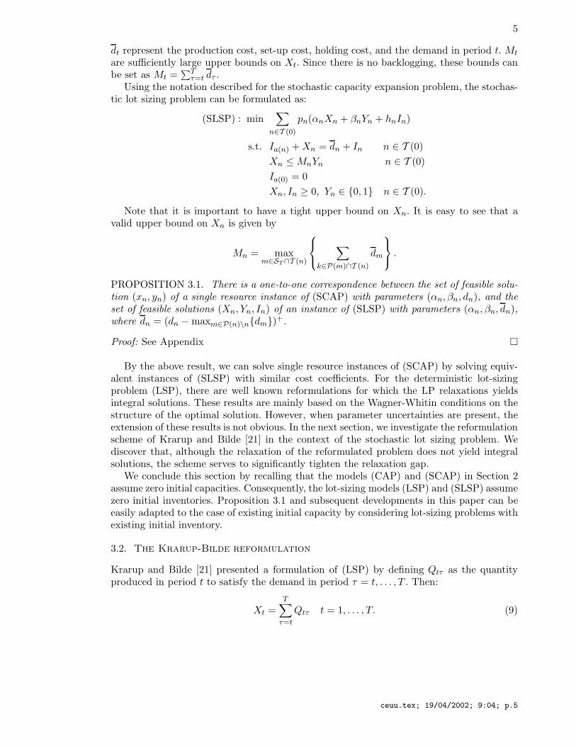
3.1. The Stochastic Lot-Sizing Problem

The deterministic uncapacitated lot sizing problem is stated as [32]:

(LSP) : minT∑

t=1

(αtXt + βtYt + htIt)

s.t. It−1 +Xt = dt + It t = 1, . . . , TXt ≤ MtYt t = 1, . . . , TI0 = 0Xt, It ≥ 0, Yt ∈ {0, 1} t = 1, . . . , T,

where Xt, It represents the production and inventory level in period t, and Yt indicateswhether a production set-up is carried out in period t. Problem parameters αt, βt, ht, and

ceuu.tex; 19/04/2002; 9:04; p.4

5

dt represent the production cost, set-up cost, holding cost, and the demand in period t. Mt

are sufficiently large upper bounds on Xt. Since there is no backlogging, these bounds canbe set as Mt =

∑Tτ=t dτ .

Using the notation described for the stochastic capacity expansion problem, the stochas-tic lot sizing problem can be formulated as:

(SLSP) : min∑

n∈T (0)

pn(αnXn + βnYn + hnIn)

s.t. Ia(n) +Xn = dn + In n ∈ T (0)Xn ≤ MnYn n ∈ T (0)Ia(0) = 0Xn, In ≥ 0, Yn ∈ {0, 1} n ∈ T (0).

Note that it is important to have a tight upper bound on Xn. It is easy to see that avalid upper bound on Xn is given by

Mn = maxm∈ST ∩T (n)

∑k∈P(m)∩T (n)

dm

.

PROPOSITION 3.1. There is a one-to-one correspondence between the set of feasible solu-tion (xn, yn) of a single resource instance of (SCAP) with parameters (αn, βn, dn), and theset of feasible solutions (Xn, Yn, In) of an instance of (SLSP) with parameters (αn, βn, dn),where dn = (dn −maxm∈P(n)\n{dm})+.

Proof: See Appendix �

By the above result, we can solve single resource instances of (SCAP) by solving equiv-alent instances of (SLSP) with similar cost coefficients. For the deterministic lot-sizingproblem (LSP), there are well known reformulations for which the LP relaxations yieldsintegral solutions. These results are mainly based on the Wagner-Whitin conditions on thestructure of the optimal solution. However, when parameter uncertainties are present, theextension of these results is not obvious. In the next section, we investigate the reformulationscheme of Krarup and Bilde [21] in the context of the stochastic lot sizing problem. Wediscover that, although the relaxation of the reformulated problem does not yield integralsolutions, the scheme serves to significantly tighten the relaxation gap.We conclude this section by recalling that the models (CAP) and (SCAP) in Section 2

assume zero initial capacities. Consequently, the lot-sizing models (LSP) and (SLSP) assumezero initial inventories. Proposition 3.1 and subsequent developments in this paper can beeasily adapted to the case of existing initial capacity by considering lot-sizing problems withexisting initial inventory.

3.2. The Krarup-Bilde reformulation

Krarup and Bilde [21] presented a formulation of (LSP) by defining Qtτ as the quantityproduced in period t to satisfy the demand in period τ = t, . . . , T . Then:

Xt =T∑

τ=t

Qtτ t = 1, . . . , T. (9)

ceuu.tex; 19/04/2002; 9:04; p.5

6

Using these variables and eliminating the inventory variables, the K-B reformulation of the(LSP) is as follows.

(RLSP) : minT∑

t=1

T∑τ=t

(αt + ht + ht+1 + . . .+ hτ−1)Qtτ +T∑

t=1

βtYt

s.t.t∑

τ=1

Qτt = dt t = 1, . . . , T

Qtτ ≤ dτYt t = 1, . . . , T ; τ = t, . . . , T

Qtτ ≥ 0, Yt ∈ {0, 1}.

PROPOSITION 3.2 (cf. [32]). The solution to the LP relaxation of (RLSP) yields 0 − 1values for the Y −variables. In addition, the image in the (X, I, Y ) space under the trans-formation (9) of all points (Q,Y ) feasible in the LP relaxation of (RLSP) produces theconvex hull of (LSP).

It thus follows that one only needs to solve the LP relaxation of (RLSP) and obtain asolution to (LSP). A number of other reformulation of (LSP) exist for which the aboveresult also holds [2, 27, 34].To extend the K-B reformulation strategy to (SLSP), let us introduce variables Qnk for

all k ∈ T (n) to indicate the part of the production Xn in node n that is used to satisfy thedemand in node k. However, in the stochastic case, the production at a node n can be usedto satisfy various demand scenarios corresponding to a particular time period. The mainobservation here is that the amount of production required at a node n is the maximumtotal amount carried over from node n to the successive periods. Thus we modify the K-Btransformation in eq. (9) as follows:

Xn = maxm∈ST ∩T (n)

∑k∈P(m)∩T (n)

Qnk

.

We can now reformulate (SLSP) as follows:

(RSLSP) : min∑

n∈T (0)

pn [αnXn + hnIn + βnYn]

s.t. Xn ≥∑

k∈P(m)∩T (n)

Qnk m ∈ ST ∩ T (n), n ∈ T (0)

∑k∈Pn

Qkn = dn n ∈ T (0)

Qnk ≤ dkYn k ∈ T (n), n ∈ T (0)Ia(n) +Xn = dn + In n ∈ T (0)Ia(0) = 0Qnk, In ≥ 0, Yn ∈ {0, 1}.

PROPOSITION 3.3. The optimal objective value of the LP relaxation of (RSLSP) is nosmaller than that of (SLSP), and it may be strictly greater.

ceuu.tex; 19/04/2002; 9:04; p.6

7

Proof: Given a feasible solution (Q,X, I, Y ) to the LP relaxation of (RSLSP), we need toshow that (X, I, Y ) is a feasible solution to the LP relaxation of (SLSP) with the sameobjective function value.We only need to show that the solution to (RSLSP) satisfies the constraints: Xn ≤ MnYn,

since all other constraints are implied. Notice that

Xn = maxm∈ST∩T (n)

∑k∈P(m)∩T (n)

Qnk

= max

m∈ST∩T (n)

∑k∈P(m)∩T (n)

dk.Qnk

dk

≤ max

m∈ST∩T (n)

∑k∈P(m)∩T (n)

dkYn

= MnYn

where the last two steps follow from the fact that Qnk ≤ dkYn, and the definition of Mn.Also note that we only consider those k ∈ P(m) ∩ T (n) for which dk > 0, since otherwiseQnk = 0.Thus the solution (X,Y, I) is feasible to (SLSP), and also has the same objective function

value. It then follows that the optimal value of the LP relaxation of (RSLSP) is no smallerthan that of (SLSP). The numerical example below shows that the value can indeed bestrictly greater. �

Example 1Consider an instance of (SLSP) with zero holding costs. The uncertain parameters evolveover the scenario tree depicted in Figure 2. The corresponding problem data are providedin Table I. The optimal IP and LP objective values of formulations (SLSP) and (RSLSP)are compared in Table II. We observe that the reformulation has very small LP relaxationgap (0.79%) in comparison to the original formulation (26.04%).

Table I. Problem Parame-ters

n αn βn dn pn

1 5 20 5 1

2 3 59 5 0.3

3 1 21 15 0.7

4 1 10 5 0.1

5 2 16 10 0.2

6 1 10 10 0.3

7 2 10 20 0.4

ceuu.tex; 19/04/2002; 9:04; p.7

8

Table II. Comparison of LP relaxation gaps

Formulation IP obj. val. LP obj. val. % Gap

(SLSP) 114.4 84.6 26.04

(RSLSP) 114.4 113.5 0.70

Unfortunately, unlike that of its deterministic counterpart, the LP relaxation of the re-formulation of (SLSP) does not yield integral solutions. This is because of the structuralproperties enjoyed by an optimal solution of (LSP) break down for the stochastic case.Table III displays the optimal solution for the numerical example. We can observe thatalthough inventory is carried in to node 3, there is still production in this node, thusIa(n)Xn = 0. Thus, the Wagner-Whitin conditions are not satisfied by an optimal solutionto the stochastic problem.

Table III. The Opti-mal Solution

n Xn Yn In

1 10 1 5

2 0 0 0

3 30 1 20

4 5 1 0

5 10 1 0

6 0 0 10

7 0 0 0

3.3. Reformulation of (SCAP)

Let us now apply the above reformulation scheme to the multi-resource capacity expansionproblem (SCAP). To see the lot-sizing substructure in this case, we introduce non-negativevariables Xn =

∑i∈I xin and binary variables zn, to denote the total capacity addition in

node n, and the decision to add capacity to any resource in node n, respectively. (SCAP)can then be written as:

min∑

n∈T (0)

pn

{∑i∈I(αinxin + βinyin)

}s.t. 0 ≤ xin ≤ Minyin n ∈ T (0); i ∈ I

yin ∈ {0, 1} n ∈ T (0); i ∈ IXn =

∑i∈I

xin n ∈ T (0)

0 ≤ Xn ≤ (∑i∈I

Min)zn n ∈ T (0)

ceuu.tex; 19/04/2002; 9:04; p.8

9∑m∈P(n)

Xm ≥ dn n ∈ T (0)

zn ∈ {0, 1} n ∈ T (0)

Note that the last three constraints of the above problem are identical to the constraintsof a single resource instance of (SCAP). Based on the variable disaggregation scheme forstochastic lot-sizing problems, the above problem can then be reformulated as:

min∑

n∈T (1)

pn

[∑i∈I(αinxin + βinyin)

]s.t. 0 ≤ xin ≤ Minyin n ∈ T (0); i ∈ I

yin ∈ {0, 1} n ∈ T (0); i ∈ IXn =

∑i∈I

xin n ∈ T (0)

Xn ≥∑

k∈T (n)∩P(m)

Qnk m ∈ ST ∩ T (n);n ∈ T (0)

∑k∈P(n)

Qkn = dn n ∈ T (0)

0 ≤ Qnk ≤ dkzn k ∈ T (n);n ∈ T (0)zn ∈ {0, 1} n ∈ T (0); i ∈ I

where dn = (dn −maxm∈P(n)\n{dm})+.Owing to the binary restrictions on zn and the constraints on Qkn, it is easily verified

that we can equivalently reformulate the above problem by substituting∑

i∈I xin for Xn,and

∑i∈I yin for zn. Thus the reformulation of the multi-resource (SCAP) is as follows:

(RSCAP) : min∑

n∈T (0)

pn

[∑i∈I(αinxin + βinyin)

]s.t. 0 ≤ xin ≤ Minyin n ∈ T (0); i ∈ I

yin ∈ {0, 1} n ∈ T (0); i ∈ I∑i∈I

xin ≥∑

k∈T (n)∩P(m)

Qnk m ∈ ST ∩ T (n);n ∈ T (0)

∑k∈P(n)

Qkn = dn n ∈ T (0)

0 ≤ Qnk ≤ dk

(∑i∈I

yin

)k ∈ T (n);n ∈ T (0)

The following example demonstrates the tightened LP relaxations obtained by the pro-posed reformulation. Further computational experiments are reported in Section 6.

ceuu.tex; 19/04/2002; 9:04; p.9

10

Example 2

Consider an instance of (SCAP) with three facilities. The uncertain parameters evolve overthe scenario tree depicted in Figure 2. The corresponding problem data are provided inTable IV. The optimal IP and LP objective values of formulations (SCAP) and (RSCAP)are compared in Table V. We observe that the reformulation has significantly smaller LPrelaxation gap (29.0%) in comparison to the original formulation (50.22%).

Table IV. Problem Parameters

n α1n α2n α3n β1n β2n β3n dn pn

0 2 1 2 10 15 5 5 1

1 1 1 1 10 30 20 15 0.3

2 3 1 2 11 5 10 10 0.7

3 1 2 1 5 10 3 5 0.1

4 2 1 1 10 3 5 10 0.2

5 2 1 3 3 10 5 10 0.3

6 1 3 2 10 5 3 20 0.4

Table V. Comparison of LP relaxation gaps

Formulation IP obj. val. LP obj. val. % Gap

(SCAP) 34.0 16.925 50.22

(RSCAP) 34.0 24.140 29.00

4. A Heuristic Strategy

In this section, we describe a heuristic strategy to construct feasible integer solutions tothe stochastic capacity expansion problem (SCAP). Note that simply rounding up thefractional values of the boolean variables (yin) in the LP relaxation solution provides afeasible integer solution. However, such a naive strategy might result in very poor solutions,possibly requiring capacity additions to be carried out in all periods. Recently, Ahmed andSahinidis [1] developed a rounding heuristic for an alternative formulation of (SCAP). Webriefly describe this heuristic strategy and adapt it to the formulation presented in thispaper.Let us consider an alternative formulation for (SCAP). Instead of defining the problem

variables over the nodes of the scenario tree, we define these over each individual scenariopath s = 1, . . . , S. A joint realization of the problem parameters corresponding to scenarios will be denoted by ωs := (ωs

1, . . . , ωsT ) where ωs

t := (αsit, β

sit, d

st ), with corresponding

probability ps. The technological constraints (2)-(4) in the deterministic problem (CAP)with the parameters ωs corresponding to scenario s will be concisely denoted by X (ωs).The decision variables corresponding to scenario s will be denoted by Xs := (Xs

1 , . . . ,XsT )

ceuu.tex; 19/04/2002; 9:04; p.10

11

with Xst := (xs

it, ysit). The objective function (1) corresponding to scenario s will be denoted

by f s(·). The decision maker cannot distinguish between the scenarios passing through thesame node at any time stage. Consequently, the feasible solutions Xs

t must satisfy:

Xs1t = Xs2

t ∀(s1, s2) ∈ n, ∀n ∈ St, ∀t = 1, . . . , T.

These conditions are known as the non-anticipativity constraints, and we shall collectivelydenote them by N . Using this notation, we can formulate the stochastic capacity expansionproblem as follows:

(SCAP′) : minS∑

s=1

psf s(Xs)

s.t. Xs ∈ X (ωs) ∩ N ∀s = 1, . . . , S

Observe that, in the absence of the non-anticipativity constraint N , the stochastic prob-lem (SCAP′) decomposes into S instances of the deterministic problem (CAP). Ahmedand Sahinidis [1] used this observation to decompose the problem across scenarios, thento construct integer solutions for each scenario subproblem, and finally to re-enforce thenon-anticipativity constraints to construct a feasible integer solution to (SCAP′). The keysteps of this heuristic are as follows. The details of the method can be found in [1].

Heuristic A:

1. Relax the integrality requirements in X (ωs) and solve the multi-stage stochastic linearprogram using standard solvers. Let X

s be the LP relaxation solution. Note that Xs ∈

N . If Xs ∈ X (ωs) stop, else go to Step 2.

2. For each scenario s, construct an integral solution fromXs by shifting capacity additions

from latter to earlier periods (see [1] for details). Let Xs be this solution. Note thatXs ∈ X (ωs). If Xs ∈ N stop, else go to Step 3.

3. Construct a solution Xs from Xs, such that Xs ∈ X (ωs) ∩ N . Note that the capacityshifting step might destroy the non-anticipativity structure of the capacity expansionvariables (xs

t ). We recover this by capacity bundling where we set xsit = maxs∈n {xs

it}for all s ∈ n, for all n ∈ St, for all t = 1, . . . , T . This guarantees that the capacityacquired in any period is the same in all scenarios of a scenario bundle. Finally, thebinary variables are rounded up accordingly.

Figure 3 illustrates the above heuristic strategy for a simple 3-period, 4-scenario example.The solutions obtained in each of the three phases of the heuristic are plotted. The heightof the rectangular blocks represent the capacity expansion bounds, and the height of fillingin the block represent the amount of capacity added in the corresponding solution. Notethat the LP relaxation solution satisfies the non-anticipativity constraints. For example, thecapacity additions in scenarios 2 and 3, in time period 2 are the same since these scenariosbelong to the same bundle. However, after capacity shifting (step 2), the non-anticipativitystructure is destroyed. The capacity bundling phase (step 3) restores the non-anticipativitystructure.It is easily verified that the scenario formulation (SCAP′) is entirely equivalent to the

tree formulation (SCAP) presented in Section 2. Thus, given any solution to one of the

ceuu.tex; 19/04/2002; 9:04; p.11

12

formulations, we can convert it to the other. Since the reformulation (RSCAP) provides atighter LP relaxation than (SCAP), we can apply the above heuristic to this solution toconstruct an integer feasible solution to (SCAP). The scheme is summarized as follows:

Heuristic B:

1. Solve the LP relaxation of (RSCAP). Let (xin, yin) denote this solution. Convert thissolution to the scenario formulation as follows. Let ns denote the leaf node in the scenariotree corresponding to scenario s. Then set xs

it := xin and ysit := yin if n ∈ P(ns) and

n ∈ St. The LP relaxation scenario solution is then Xs := (xs

it, ysit).

2. Apply steps 2 and 3 in Heuristic A to construct a heuristic solution to the scenarioformulation Xs = (xs

it, ysit) from the LP relaxation solution X

s.

3. Construct a heuristic solution to the tree formulation (SCAP) as follows: set xin := xsit

and yin := ysit if n ∈ P(ns) and n ∈ St.

Ahmed and Sahinidis [1] proved that Heuristic A produces a feasible solution to (SCAP′).From the equivalence of the two formulations, the following result then follows immediately.

PROPOSITION 4.1. Heuristic B produces a feasible solution to (SCAP).

The proposed heuristic can be easily improved by only shifting to periods that offer acost benefit. Furthermore, the strategy can potentially be integrated with other heuristicmethods such as those proposed by Fong and Srinivasan [16] and Li and Tirupati [23]. Suchimprovements will only produce better quality solutions. Under some standard assumptionson the parameter distributions, Ahmed and Sahinidis [1] showed that Heuristic A is asymp-totically optimal in the number of time periods. This result implies that, as the problem sizeincreases, the quality of the heuristic solution also increases and eventually, for sufficientlylarge problem sizes, the heuristic provides optimal solutions. Intuitively, if the demands arenot expected to vary widely (for example, if they have bounded moments), the heuristic canbe expected to have carried out enough capacity expansions in the early periods to satisfythe most of the demand. From the equivalence of the two formulations, Heuristic B alsopossesses this attractive property.

5. A Branch & Bound Algorithm

As mentioned earlier, currently there are no practical general purpose solution algorithms formulti-stage stochastic integer programs. A pioneering effort in this area is that of Carøe andSchultz [9] who proposed a branch and bound scheme coupled with Lagrangian relaxationfor scenario formulations of multi-stage stochastic integer programs. In this scheme, theLagrangian dual obtained by relaxing the non-anticipativity constraints in the scenarioformulation is solved to obtain lower bounds. Relaxing the non-anticipativity constraintsdecomposes the problem and allows each scenario sub-problem to be solved independently.A subgradient approach is then used to improve the dual multipliers. To close the dualitygap the authors propose branching on the integer variables. In [8] and [9], the authorspresent computational results using this algorithm for two-stage problems. Although themethod is theoretically applicable to the multi-stage case, the authors acknowledge that

ceuu.tex; 19/04/2002; 9:04; p.12

13

owing to the increased dimensionality of the Lagrangian dual and the branching variables,several issues regarding a successful implementation of such an approach for the multi-stagecase remain open.In this paper, we propose to solve (SCAP) by enhancing the standard integer program-

ming branch and bound algorithm with the problem specific reformulation technique andheuristic strategy described in Sections 3 and 4. In this scheme, we solve the LP relaxationof the reformulated problem (RSCAP) to obtain tight lower bounds. Standard stochasticlinear programming decomposition schemes, such as those implemented in solvers such as[19], can be used to solve these relaxations. As an upper bounding routine, Heuristic B(cf. Section 4) is used to obtain good quality feasible integer solutions. Conventional integerprogramming rules are used for branching.A potential advantage of the proposed method over that of Carøe and Schultz [9] from

an implementation point of view is that the lower bound is obtained by linear program-ming rather than computationally expensive subgradient methods to solve the Lagrangiandual. Furthermore, the number of branching variables is fewer. The scenario formulationof (SCAP′) that would be used in the Carøe and Schultz algorithm requires |I| × T × Sbinary variables, whereas the tree formulation (SCAP) requires |I|×|T (0)| binary variables;and |T (0)| < T × S. For example, a binary scenario tree with T periods has S = 2T−1,and |T (0)| = (2T − 1). Then if T > 1, we have |T (0)| < T × 2T−1. On the other hand,the Lagrangian bounding scheme of Carøe and Schultz is independent of any specializedproblem structure and provides very tight lower bounds for most problems.

6. Computational Results

In this section, we provide some computational experience using the solution strategydescribed in Section 5 to solve a set of 16 small instances of the multi-stage stochasticcapacity expansion problem (SCAP). A ternary scenario tree was assumed with the uncer-tain parameters jointly realizing as one of three sets of values in each period. Problems weregenerated by varying the number of time periods from 2 to 5 and the number of facilities from1 to 4. Data for the problem instances are available from the authors. Table VI presentsthe time periods, tree size, number of scenarios, number of facilities, and the number ofbinary variables, continuous variables, and rows in the original formulation (SCAP) and itsreformulation (RSCAP). Note that although the reformulation introduces a large numberof additional continuous variables and rows, the number of binary variables is same in bothmodels.We first investigate the strength of the LP relaxation gap of (RSCAP), and then the

performance of the proposed branch and bound algorithm. All computations were carriedout on an IBM RS/6000 Model 590 Workstation with 512 Mb RAM and a 66MHz processor.CPLEX 6.6 was used to the solve the linear and integer programs.

6.1. Comparison of LP Relaxation Gaps

Table VII compares the gap (from the optimal integer solution) and the CPU seconds forthe LP relaxation of the original formulation (SCAP) and the reformulation (RSCAP). Asexpected, the reformulation requires higher CPU time, but provides significantly better LPrelaxation bounds.

ceuu.tex; 19/04/2002; 9:04; p.13

14

Table VI. Problem Dimensions

(SCAP) (RSCAP)

No. T |T (0)| S |I| Bin. Cont. Rows Bin. Cont. Rows

P 2 1 2 4 3 1 4 4 8 4 14 24

P 2 2 2 4 3 2 8 8 12 8 18 28

P 2 3 2 4 3 3 12 12 16 12 22 32

P 2 4 2 4 3 4 16 16 20 16 26 36

P 3 1 3 13 9 1 13 13 26 13 104 141

P 3 2 3 13 9 2 26 26 39 26 117 154

P 3 3 3 13 9 3 39 39 52 39 130 167

P 3 4 3 13 9 4 52 52 65 52 143 180

P 4 1 4 40 27 1 40 40 80 40 860 951

P 4 2 4 40 27 2 80 80 120 80 900 991

P 4 3 4 40 27 3 120 120 160 120 940 1031

P 4 4 4 40 27 4 160 160 200 160 980 1071

P 5 1 5 121 81 1 121 121 242 121 7502 7350

P 5 2 5 121 81 2 242 242 363 242 7623 7471

P 5 3 5 121 81 3 363 363 484 363 7744 7592

P 5 4 5 121 81 4 484 484 605 484 7865 7713

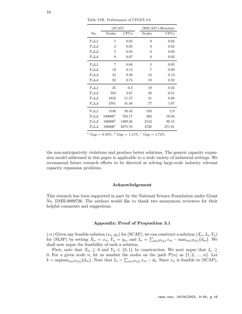
6.2. Performance of the Proposed Branch and Bound Algorithm

The proposed branch and bound algorithm was implemented by integrating Heuristic Bwith the CPLEX 6.6 MIP solver, and applying the algorithm to the reformulation (RSCAP).Table VIII compares the performance of the proposed method ((RSCAP) + Heuristic) toa straightforward application of the CPLEX 6.6 MIP solver on the original formulation(SCAP). A node limit of 100, 000 was imposed and the CPLEX default relative toleranceof 0.0001 was used. As can be observed from Table VIII, the proposed enhancements offersignificant reductions in the number of nodes and CPU seconds. The three largest problemsin the set could not be solved within the prescribed resource limits using the straightforwardCPLEX implementation.

7. Conclusions and Future Research

The key contributions of this paper are the following:

− We have proposed a multi-stage stochastic integer programming formulation for ageneral multi-resource capacity expansion problem under uncertainty.

− A reformulation scheme has been developed by exploiting special lot-sizing sub-structurein the problem. The proposed reformulation offers significantly tighter LP relaxationgaps than the original formulation.

ceuu.tex; 19/04/2002; 9:04; p.14

15

Table VII. LP Relaxation Gaps

(SCAP) (RSCAP)

No. % Gap CPUs % Gap CPUs

P 2 1 22.64 0.00 2.63 0.00

P 2 2 28.79 0.01 5.22 0.01

P 2 3 34.19 0.01 13.57 0.00

P 2 4 35.14 0.00 14.10 0.01

P 3 1 21.08 0.00 2.69 0.03

P 3 2 26.43 0.01 4.33 0.03

P 3 3 31.98 0.01 12.39 0.03

P 3 4 33.31 0.00 13.08 0.03

P 4 1 19.29 0.02 2.39 0.11

P 4 2 24.44 0.02 3.01 0.13

P 4 3 30.02 0.03 9.44 0.13

P 4 4 31.49 0.04 10.10 0.14

P 5 1 19.24 0.06 2.75 0.71

P 5 2 24.03 0.11 3.03 0.78

P 5 3 29.45 0.14 8.61 0.88

P 5 4 31.00 0.20 9.13 0.97

Average 27.66 0.04 7.28 0.25

− We have modified a recently proposed heuristic strategy for scenario based formulationsof capacity expansion problems to be applicable to the formulation presented in thispaper.

− We have proposed enhancing standard integer programing branch and bound algo-rithms by integrating the reformulation scheme and the heuristic strategy to solve theproblem to global optimality.

− We have presented computational results demonstrating the effectiveness of the refor-mulation and the proposed branch and bound algorithm.

The results in this paper pave the way for a number of future research avenues. Weassumed that the capacity expansion bounds were large enough, making the problem “un-restricted” and allowing the exploitation of the uncapacitated lot-sizing substructure. Forthe restricted case, recent results on capacitated lot-sizing problems [28] can be investigatedfor possible extensions. The heuristic strategy also has considerable room for improvement.Note that by fixing the solution corresponding to a parent node of the scenario tree aftera single pass of the heuristic, we can decouple the problems corresponding to the childsub-trees. The heuristic can then be applied recursively to these sub-trees. This multi-passversion of the heuristic can offer significantly better solutions. Furthermore, in the capacityshifting phase of the heuristic, the non-anticipativity constraints are relaxed without anypenalties. Incorporating appropriate Lagrange multipliers in the objective can help reduce

ceuu.tex; 19/04/2002; 9:04; p.15

16

Table VIII. Performance of CPLEX 6.6

(SCAP) (RSCAP)+Heuristic

No. Nodes CPUs Nodes CPUs

P 2 1 1 0.02 0 0.02

P 2 2 2 0.05 0 0.02

P 2 3 5 0.04 0 0.03

P 2 4 9 0.07 0 0.02

P 3 1 7 0.04 5 0.05

P 3 2 19 0.14 7 0.09

P 3 3 45 0.39 12 0.13

P 3 4 82 0.74 19 0.22

P 4 1 35 0.3 19 0.32

P 4 2 563 2.67 28 0.51

P 4 3 1822 11.57 41 0.88

P 4 4 4701 41.48 77 1.87

P 5 1 1536 20.43 193 5.9

P 5 2 100000a 784.17 492 16.94

P 5 3 100000b 1409.26 2142 90.15

P 5 4 100000c 2975.70 4728 271.91

a Gap = 0.58%, b Gap = 1.11%, c Gap = 1.74%.

the non-anticipativity violations and produce better solutions. The generic capacity expan-sion model addressed in this paper is applicable to a wide variety of industrial settings. Werecommend future research efforts to be directed at solving large-scale industry relevantcapacity expansion problems.

Acknowledgement

This research has been supported in part by the National Science Foundation under GrantNo. DMII-0099726. The authors would like to thank two anonymous reviewers for theirhelpful comments and suggestions.

Appendix: Proof of Proposition 3.1

(⇒) Given any feasible solution (xn, yn) for (SCAP), we can construct a solution (Xn, In, Yn)for (SLSP) by setting Xn = xn, Yn = yn, and In =

∑m∈P(n) xm − maxm∈P(n){dm}. We

shall now argue the feasibility of such a solution.First, note that Xn ≥ 0 and Yn ∈ {0, 1} by construction. We next argue that In ≥

0. For a given node n, let us number the nodes on the path P(n) as {1, 2, . . . , n}. Letk = argmaxm∈P(n){dm}. Note that In =

∑m∈P(n) xm − dk. Since xn is feasible in (SCAP),

ceuu.tex; 19/04/2002; 9:04; p.16

17

we have, for the k-th node,∑k

m=1 xm − dk ≥ 0. Since xm ≥ 0 for all m, it then followsIn =

∑km=1 xm − dk +

∑nm=k+1 xm ≥ 0.

It now remains to check the for the inventory balance constraints in (SLSP). For a givennode n, the left-hand side of this constraint is given by:

Ia(n) +Xn =∑

m∈P(n)\nxm − max

m∈P(n)\n{dm}+ xn

=∑

m∈P(n)

xm − maxm∈P(n)\n

{dm}.

The right-hand side of this constraint is:

dn + In = (dn − maxm∈P(n)\n

{dm})+ +∑

m∈P(n)

xm − maxm∈P(n)

{dm}.

If dn > maxm∈P(n)\n{dm}, then maxm∈P(n){dm} = dn, and both sides of the inventory bal-ance constraint are equal. Otherwise, (dn−maxm∈P(n)\n{dm})+ = 0 and maxm∈P(n){dm} =maxm∈P(n)\n{dm}, and once again both sides of the constraint are equal. Thus the con-structed solution is feasible to (SLSP).

(⇐) Given a feasible solution (Xn, In, Yn) to (SLSP), we can construct a solution (xn, yn) to(SCAP) by setting xn = Xn, and yn = Yn. We next argue the feasibility of such a solution.Note that xn ≥ 0 and yn ∈ {0, 1} by construction. Since there are no initial inventories,

by summing up the inventory balance constraints in (SLSP) for all m ∈ P(n), we have∑m∈P(n) Xn ≥∑

m∈P(n) dm, implying∑

m∈P(n) xn ≥∑m∈P(n) dm. It remains to argue that∑

m∈P(n) dm ≥ dn or ∑m∈P(n)

(dm − maxk∈P(m)\m

{dk})+ ≥ dn. (10)

For a given node n, let us number the nodes on the path P(n) as {1, 2, . . . , n}. Then, theleft-hand side of (10) is

n∑m=1

(dm −max{d1, . . . , dm−1})+ = d1 + (d2 − d1)+ + (d3 −max{d1, d2})+ + . . .

+ (dn −max{d1, . . . , dn−1})+

= max{d1, d2, . . . , dn}.

Since max{d1, d2, . . . , dn} ≥ dn, inequality (10) holds for all n. Thus the constructed solutionis feasible to (SCAP). �

References

1. S. Ahmed and N. V. Sahinidis. An asymptotically optimal heuristic for a stochastic capacity expansionproblem. Working paper, Department of Chemical Engineering, University of Illinois, 2000.

2. I. Barany, T. Van Roy, and L. A. Wolsey. Uncapacitated lot-sizing: The convex hull of solutions.Mathematical Programming Study, 22:32–43, 1984.

ceuu.tex; 19/04/2002; 9:04; p.17

18

3. J. C. Bean, J. L. Higle, and R. L. Smith. Capacity expansion under stochastic demands. OperationsResearch, 40:S210–S216, 1992.

4. O. Berman and Z. Ganz. The capacity expansion problem in the service industry. Computers &Operations Research, 21:557–572, 1994.

5. O. Berman, Z. Ganz, and J. M. Wagner. A stochastic optimization model for planning capacityexpansion in a service industry under uncertian demand. Naval Research Logistics, 41:545–564, 1994.

6. S. Bermon and S. Hood. Capacity optimization planning system (CAPS). Interfaces, 29:31–50, 1999.7. J. R. Birge and F. Louveaux. Introduction to Stochastic Programming. Springer, New York, NY, 1997.8. C. C. Carøe. Decomposition in stochastic integer programming. PhD thesis, University of Copenhagen,

1998.9. C. C. Carøe and R. Schultz. Dual decomposition in stochastic integer programming. Operations

Research Letters, 24:37–45, 1999.10. S-G. Chang and B. Gavish. Telecommunications network topological design and capacity expansion:

Formulations and algorithms. Telecommunication Systems, 1:99–131, 1993.11. Z-L. Chen, S. Li, and D. Tirupati. A scenario based stochastic programming approach for technology

and capacity planning. To appear in Computers & Operations Research, 2001.12. M. H. A. David, M. A. H. Dempster, S. P. Sethi, and D. Vermes. Optimal capacity expansion under

uncertainty. Advances in Applied Probability, 19:156–176, 1987.13. J. Dupacova, G. Consigli, and S. W. Wallace. Scenarios for multi-stage stochastic programs. Working

paper. Norwegian University of Science and Technology.URL: http://www.iot.ntnu.no/iok html/users/sww/reports.htm, 2000.

14. G. D. Eppen, R. K. Martin, and L. Schrage. A scenario approach to capacity planning. OperationsResearch, 37:517–527, 1989.

15. C. H. Fine and R. M. Freund. Optimal investment in product-flexible manufacturing capacity.Management Science, 36:449–466, 1990.

16. C. O. Fong and V. Srinavasan. The multiregion dynamic capacity expansion problem: Part II.Operations Research, 29:800–816, 1981.

17. J. Freidenfelds. Capacity expansion when demand is a birth-death random process. OperationsResearch, 28:712–721, 1980.

18. K. Høyland and S. W. Wallace. Generating scenario trees for multi-stage decision problems. To appearin Management Science, 2000.

19. IBM Corporation. IBM Stochastic Solutions.URL: http://www6.software.ibm.com/es/oslv2/features/stoch.htm, 1998.

20. P. Kall and S. W. Wallace. Stochastic Programming. John Wiley and Sons, Chichester, England, 1994.21. J. Krarup and O. Bilde. Plant location, set covering and economic lot size: An o(mn) algorithm for

structured problems. In Optimierung bei Graphentheoretischen und ganzzahligen Problemen, Collatzet al. (eds.), International Series of Numerical Mathematics, Birkhauser-Verlag, 36:155–180, 1977.

22. M. Laguna. Applying robust optimization to capacity expansion of one location in telecommunicationswith demand uncertainty. Management Science, 44:S101–S110, 1998.

23. S. Li and D. Tirupati. Dynamic capacity expansion problem with multiple products: technologyselection and timing of capacity additions. Operations Research, 42:958–976, 1994.

24. M. L. Liu and N. V. Sahinidis. Optimization in process planning under uncertainty. Industrial &Engineering Chemistry Research, 35:4154–4165, 1996.

25. A. S. Manne. Capacity expansion and probabilistic growth. Econometrica, 29:632–649, 1961.26. A.S. Manne, editor. Investments for Capacity Expansion. The MIT press, Cambridge, MA, 1967.27. R. K. Martin. Generating alternative mixed-integer programming models using variable redefinition.

Operations Research, 35:820–831, 1987.28. A. J. Miller. Polyhedral Approaches to Capacitated Lot-Sizing Problems. PhD thesis, Georgia Institute

of Technology, 1999.29. J. M. Mulvey. Generating scenario for the towers perrin investment system. Interfaces, 26:1–13, 1996.30. F. H. Murphy, S. Sen, and A. L. Soyster. Electric utility expansion planning in the presence of existing

capacity: A nondifferentiable, convex programming approach. Computers & Operations Research,14:19–31, 1987.

31. F. H. Murphy and H. J. Weiss. An approach to modeling electric utility capacity expansion planning.Naval Research Logistics, 37:827–845, 1990.

ceuu.tex; 19/04/2002; 9:04; p.18

19

32. G. L. Nemhauser and L. A. Wolsey. Integer and Combinatorial Optimization. John Wiley & Sons,1988.

33. G. Ch. Pflug. Scenario tree generation for multiperiod financial optimization by optimal discretization.Mathematical Programming, Series B. 89:251–271, 2001.

34. Y. Pochet and L. A. Wolsey. Lot-size models with backlogging: Strong reformulations and cuttingplanes. Mathematical Programming, 40:317–335, 1988.

35. S. Rajagopalan, M. R. Singh, and T. E. Morton. Capacity expansion and replacement in growingmarkets with uncertain technological breakthroughs. Management Science, 44:12–30, 1998.

36. N. V. Sahinidis and I. E. Grossmann. Reformulation of the multiperiod milp model for capacityexpansion of chemical processes. Operations Research, 40, Supp. No. 1:S127–S144, 1992.

37. I. Saniee. An efficient algorithm for the multiperiod capacity expansion of one location intelecommunications. Operations Research, 43:187–190, 1995.

38. J. M. Swaminathan. Tool capacity planning for semiconductor fabrication facilities under demanduncertainty. European Journal of Operational Research, 120:545–558, 2000.

ceuu.tex; 19/04/2002; 9:04; p.19

20

n

)(n�

)(n�

0

s = 1

s = 2

s = S

.

.

.

t = 1 t = T. . .

)(na

t = t n

nt�

Figure 1. The Scenario Tree Notation

✒✑�✏

✒✑�✏

✒✑�✏

✒✑�✏

✒✑�✏

✒✑�✏

✑✑

✑✑✸✟✟✟✟✟✯

�

◗◗

◗◗�

✒✑�✏

✲

t=2

�

0

1

2

3

4

5

6

t=3t=1

Figure 2. The Scenario Tree for Example 1

ceuu.tex; 19/04/2002; 9:04; p.20

21

Figure 3. The Heuristic Strategy

ceuu.tex; 19/04/2002; 9:04; p.21

ceuu.tex; 19/04/2002; 9:04; p.22