AN ABSTRACT OF A THESIS

PREDICTIVE ANALYSIS OF WIRELESS NETWORK BEHAVIORFROM PACKET DROP DATA USING RANDOM MATRIX THEORY

Aribido Oluwaseun Joseph

Master of Science in Electrical and Computer Engineering

Random Matrix Theory (RMT) has received accredited research attention inrecent times due to the universality of its tools for application across wide spatialdisciplines such as Quantum Physics, Biology, Multivariate Statistics and recently,Wireless Communication - especially for Multi-user MIMO. On another hand, thereis a burgeoning trend to find a model for the emerging discipline of Big-Data whichcoincides with the pertinent need to find suitable statistical framework in the samedomain. To leverage on the tools of RMT while analyzing Big-data, recent techniquesin RMT are used to monitor and predict the behavior of a single-cell wireless networkfrom a Big-data perspective using packet drop data collected from the network.

A network simulation is setup in OPNET Modeler 17.5 environment featuring250 Mobile nodes together with a central base station in a 3000× 3000 square-meterarea. Packet drop data is collected from each mobile node during down link trans-mission. Each packet drop is treated as a random variable and filled into the entriesof a matrix. The eigenvalue distribution of the matrix is investigated against estab-lished random matrix theories such as Marcenko-Pastur (MP) law, spiked eigenvaluemodels, and the ring law. Three consecutive scenarios are run in OPNET: First,shadow fading is enabled. Kernel Density Estimation is used to compare the proba-bility density function of the packet drop matrix against MP-distribution. The resultshows that the entries of the matrix are independent, not necessarily identical andthe ring-law also confirms this. In the second scenario, anonymous interference isintroduced into the network using a network Jammer. An eigenvalue spike in theeigenvalue spectrum is observed together with a shrinkage of eigenvalues towards theinner-radius of the unit ring. In the third scenario, four sources with independentjamming waveforms are added to the network and the packet drop matrix analyzedagain. The eigenvalue spectrum showed four eigenvalue spikes corresponding to fourjammers, with further shrinkage of eigenvalues towards the centers of the unit ring-showing much reduced independence between the rows of packet drop matrix. Theseresults are discussed in detail using RMT tools and an approximate model is foundfor the second scenario. Future research direction in the regard of this work is alsogiven.

PREDICTIVE ANALYSIS OF WIRELESS NETWORK BEHAVIOR

FROM PACKET DROP DATA USING RANDOM MATRIX THEORY

A Thesis

Presented to

the Faculty of the Graduate School

Tennessee Technological University

by

Aribido Oluwaseun Joseph

In Partial Fulfillment

of the Requirements for the Degree

MASTER OF SCIENCE

Electrical and Computer Engineering

Dec, 2014

Copyright c© Aribido Oluwaseun Joseph, 2014

All rights reserved

ii

CERTIFICATE OF APPROVAL OF THESIS

PREDICTIVE ANALYSIS OF WIRELESS NETWORK BEHAVIOR

FROM PACKET DROP DATA USING RANDOM MATRIX THEORY

by

Aribido Oluwaseun Joseph

Graduate Advisory Committee:

Dr. Robert Qiu, Chairperson date

Dr. Robert Qiu, Co-Chair date

Dr. Adam Anderson date

Dr. Mahmoud Mohammed date

Approved for the Faculty:

Francis OtuonyeAssociate Vice-President forResearch and Graduate Studies

Date

iii

DEDICATION

This Thesis is dedicated to my parents - who taught me the rudiments of life;

and to my Fiancee, Emike whose love replenishes my grand resolve.

iv

ACKNOWLEDGMENTS

My greatest appreciation goes to my lord and savior, Jesus Christ for his love

and ultimate sacrifice for me. I wish to give an unreserved gesture of appreciation

to my supervisor and adviser, Dr. Robert Caiming Qiu for his keen and visionary

research sense. I’ve not met yet a more motivated researcher as Dr. Qiu, his drive for

excellence is contagious. I also extend deep appreciation for Dr. Terry N. Guo, for his

patience and invaluable effort to painstakingly oversee every detail of this research.

In addition, I dearly appreciate the veritable support and counsel I received

from the members of my graduate committee: Dr. Adam Anderson and Dr. Mah-

moud Mohamed. Thank you so much. Also pertinent on my lit of appreciation is my

fellow graduate colleagues: Alex C. Zhang, Feng Lin and Brett Witherspoon for mak-

ing the lab warm with our business. A profound gratitude goes to my pals: Wadzani

Dauda, Adeniyi Babalola, Jojo France-Mensah, Dare Oladapo, Micheal Adenson, Es-

eme Sota, Helen, Tosin Owoseni, Muchy Ahiakwo and a host of acquaintances for the

rides to school, the insightful arguments, the prayer sessions and their contributions

to my life in one way or the other. I am very grateful.

I must not forget to dearly acknowledge my parents: Dr. and Mrs Aribido

together with Mrs Idalu for the love and care they have shown me thus far. It’s a

privilege to have you all as parents. I recall with gratitude, the love and support of

Tope, Rita, Deji, Pascal and David, my siblings. I love you all.

I reserve here an immeasurable chunk of gratitude to my wife and lover,

princess Rosemary Emike Idalu for her companionship and love all through my re-

search work. Your patience, smiles and friendship kept me going at every twist

v

and turn. Lastly, I appreciate the love and fellowship of my family at Life Church,

Cookeville especially the adult leaders at the Edge, you are awesome.

With Regards, Joseph

vi

TABLE OF CONTENTS

Page

LIST OF TABLES . . . . . . . . . . . . . . . . . . . . . . . . . . . . . . . . . xi

LIST OF FIGURES . . . . . . . . . . . . . . . . . . . . . . . . . . . . . . . . xii

Chapter

1. INTRODUCTION . . . . . . . . . . . . . . . . . . . . . . . . . . . . . 1

1.1 A BRIEF REVIEW . . . . . . . . . . . . . . . . . . . . . . . 1

1.2 MOTIVATION FOR THIS WORK . . . . . . . . . . . . . . 4

1.3 RESEARCH METHODLOGY . . . . . . . . . . . . . . . . . 5

1.4 ORGANIZATION OF THE THESIS . . . . . . . . . . . . . 6

2. LITERATURE SURVEY ON RANDOM MATRIX THEORY FORWIRELESS NETWORKS . . . . . . . . . . . . . . . . . . . . . . . . 7

2.1 LIMITING SPECTRAL DISTRIBUTIONS OF LARGERANDOM MATRICES . . . . . . . . . . . . . . . . . . . . . 8

2.1.1 The Semi-Circular Law . . . . . . . . . . . . . . . . . . . 8

2.1.2 The Circular Law . . . . . . . . . . . . . . . . . . . . . . 9

2.1.3 The Marcenko-Pastur Law . . . . . . . . . . . . . . . . . 10

2.2 RECENT RANDOM MATRIX TECHNIQUES . . . . . . . 12

2.2.1 Free Probability of Random Matrices . . . . . . . . . . . 12

R-Transform . . . . . . . . . . . . . . . . . . . . . . . . . . 15

S-Transform . . . . . . . . . . . . . . . . . . . . . . . . . . 16

vii

viii

Appendices Page

2.2.2 Perturbed Sample Covariance Matrices . . . . . . . . . . 18

The Ring Law . . . . . . . . . . . . . . . . . . . . . . . . . 20

Outliers outside the Ring Law . . . . . . . . . . . . . . . . . 21

2.2.3 Kernel Density Estimation . . . . . . . . . . . . . . . . . 23

3. SIMULATION SETUP AND DATA COLLECTION . . . . . . . . . . 26

3.1 OPNET BASICS . . . . . . . . . . . . . . . . . . . . . . . . 26

3.2 WHY OPNET . . . . . . . . . . . . . . . . . . . . . . . . . . 28

3.3 OPNET MODELER ENVIRONMENT . . . . . . . . . . . . 30

3.3.1 Node Editor . . . . . . . . . . . . . . . . . . . . . . . . . 31

3.3.2 Process Editor . . . . . . . . . . . . . . . . . . . . . . . 32

3.3.3 Project Editor . . . . . . . . . . . . . . . . . . . . . . . . 34

3.4 SIMULATION SETUP . . . . . . . . . . . . . . . . . . . . . 35

3.4.1 Channel Model . . . . . . . . . . . . . . . . . . . . . . . 38

3.5 PACKET DROP DATA COLLECTION . . . . . . . . . . . 38

3.5.1 Shadowing enabled in the network . . . . . . . . . . . . 41

3.5.2 One Jammer is placed in the network . . . . . . . . . . . 43

3.5.3 Four Jammers are placed in the network . . . . . . . . . 45

4. DATA ANALYSIS BY CASE STUDIES . . . . . . . . . . . . . . . . . 50

4.1 INTRODUCTION . . . . . . . . . . . . . . . . . . . . . . . 50

4.2 MODELING LARGE PACKET DROP RANDOM MATRICBY CASE STUDIES . . . . . . . . . . . . . . . . . . . . . . . 51

4.3 CASE 1: SHADOWING ENABLED . . . . . . . . . . . . . 51

ix

Appendices Page

4.3.1 Case 1 - Discussion . . . . . . . . . . . . . . . . . . . . . 54

4.4 CASE 2: ONE JAMMER IS PLACED IN THE NETWORK 55

4.4.1 Case 2 - Discussion . . . . . . . . . . . . . . . . . . . . . 57

Spiked Model for Packet Drop Data with One AnonymousInterference . . . . . . . . . . . . . . . . . . . . . . . . . 59

4.5 CASE 3: FOUR JAMMERS ARE PLACED IN THENETWORK . . . . . . . . . . . . . . . . . . . . . . . . . . . 61

4.5.1 Case 3 - Discussion . . . . . . . . . . . . . . . . . . . . . 62

5. SUMMARY AND CONCLUSION . . . . . . . . . . . . . . . . . . . . . 67

5.1 SUMMARY IN BRIEF . . . . . . . . . . . . . . . . . . . . . 67

5.1.1 Some Application of Results . . . . . . . . . . . . . . . . 69

5.2 FURTHER RESEARCH ON THIS WORK . . . . . . . . . . 71

5.2.1 Separation of Eigenvalue spectrum . . . . . . . . . . . . 71

5.2.2 Distribution of eigenvalue spikes . . . . . . . . . . . . . . 72

5.2.3 Localization of Jamming nodes in large complex networks 72

5.3 CONCLUSION . . . . . . . . . . . . . . . . . . . . . . . . . 73

A. MATLAB CODE FOR FIGURES IN THIS WORK . . . . . . . . . . . . 75

.1 MATLAB CODES FOR CHAPTER 2 . . . . . . . . . . . . . 76

.1.1 Wigner’s Semi-circle (Fig. 2.1) . . . . . . . . . . . . . . . 76

.1.2 Full-Circle Law (Fig. 2.2) . . . . . . . . . . . . . . . . . . 76

.1.3 Marcenko-Pastur Distribution (Fig. 2.3) . . . . . . . . . . 77

.1.4 Marcenko-Pastur Law with Outliers (Fig. 2.6) . . . . . . . 77

x

Appendices Page

.1.5 Haar distribution (Fig. 2.5) . . . . . . . . . . . . . . . . . 79

.1.6 Distribution of Eigenvalues within the Unit Ring (fig. 2.7) 79

B. NETWORK FIGURES . . . . . . . . . . . . . . . . . . . . . . . . . . . . 81

VITA . . . . . . . . . . . . . . . . . . . . . . . . . . . . . . . . . . . . . . . . 84

BIBLIOGRAPHY . . . . . . . . . . . . . . . . . . . . . . . . . . . . . . . . . 85

LIST OF TABLES

Table Page

3.1 OPNET 17.5 Interface . . . . . . . . . . . . . . . . . . . . . . . . . . . 26

3.2 Comparison of Popular Network Simulators. . . . . . . . . . . . . . . . 28

3.3 Simulators used in IEEE Journals and Conference Papers Published from2007 TO 2009 [1] . . . . . . . . . . . . . . . . . . . . . . . . . . . . . 29

3.4 Simulation Parameters for Mobile User and Base-Station Profile . . . . 37

3.5 Baseline configurations for IMT-Advanced. . . . . . . . . . . . . . . . . 39

3.6 Simulation Parameters for jammer’s profile used in OPNET (µ = mean,σ = standard deviation) . . . . . . . . . . . . . . . . . . . . . . . . . 47

xi

LIST OF FIGURES

Figure Page

2.1 Histogram of Eigenvalues . . . . . . . . . . . . . . . . . . . . . . . . . . 9

2.2 Eigenvalues of XN with N = 1000 . . . . . . . . . . . . . . . . . . . . 10

2.3 The Spectral distribution of 1nXXH with X ∈ CN×n when n = 1000,

N = 500 and c = N/n. The blue line is Marcenko-Pastur Law. . . . . 11

2.4 The Spectral distribution of 1nXXH with X ∈ CN×n when n = 1000,

N = 100 and c = N/n. The blue line is Marcenko-Pastur Law. . . . . 12

2.5 Haar Distribution. Notice that all eigenvalues lie on the unit circle. SeeMatlab code at Appendix A .1.5 . . . . . . . . . . . . . . . . . . . . 14

2.6 Marcenko-Pastur Law with outliers. . . . . . . . . . . . . . . . . . . . . 20

2.7 Distribution of Eigenvalues within the unit ring. See Appendix A .1.6 forMatlab code . . . . . . . . . . . . . . . . . . . . . . . . . . . . . . . . 21

2.8 The Ring Law with 3 Outliers. The Outliers are due to perturbation bylow-rank matrix F with eigenvalues outside the unit ring . . . . . . . 22

2.9 Kernel density Estimation when for h=0.02. Notice that the densityfunction is estimated but with spurts. . . . . . . . . . . . . . . . . . 24

2.10 Kernel density Estimation when for h=0.09 On Increasing h to 0.09, theoriginal density function is well estimated with the kernel density plot 25

3.1 OPNET Node Editor Interface. . . . . . . . . . . . . . . . . . . . . . . 31

3.2 OPNET Process Editor Interface. . . . . . . . . . . . . . . . . . . . . . 33

3.3 Obeject Palette tree. . . . . . . . . . . . . . . . . . . . . . . . . . . . . 35

3.4 Network Topology in OPNET. . . . . . . . . . . . . . . . . . . . . . . . 36

3.5 Discrete Event Simulation Parameters for the Topology used in this work 40

xii

xiii

Figure Page

3.6 Packet Drop Signature for selected nodes in all 10 clusters whenShadowing is enabled in the network . . . . . . . . . . . . . . . . . . 42

3.7 Network Topology Diagram when One Jammer is introduced into thenetwork . . . . . . . . . . . . . . . . . . . . . . . . . . . . . . . . . . 43

3.8 Jamming Waveform of Pulsed Jammer introdcued into the network. . . 44

3.9 Notice that the Pulses of the Jammer causes the packet drop signatureto vary in a similar fashion to the jamming waveform . . . . . . . . . 44

3.10 Packet Drops signature after one jammer is introduced into the network.Notice that nodes father from the cluster have lower packet drop rate.Nodes in Cluster 7 and 8 show higher variance and mean of packet dropand routine spikes in packet drop rate . . . . . . . . . . . . . . . . . 45

3.11 Modified Process Model of OPNET’s Pulsed Jammer . . . . . . . . . . 46

3.12 Pulsed Waveform of Jammer1 and corresponding packet drop profile . . 47

3.13 Pulsed Waveform of Jammer2 and corresponding packet drop profile . . 48

3.14 Pulsed Waveform of Jammer3 and corresponding packet drop profile . . 48

3.15 Pulsed Waveform of Jammer4 and corresponding packet drop profile . . 48

3.16 Network Topology with 4 Jammers Introduced . . . . . . . . . . . . . . 49

4.1 Marcenko-Pastur Distribution Vs Histogram of Eigenvalues of S =1√nXXH where n = 400 . . . . . . . . . . . . . . . . . . . . . . . . . 52

4.2 Marcenko-Pastur Distribution Vs KDE of the spectral distribution ofS = 1√

nXSX

HS where n = 400 . . . . . . . . . . . . . . . . . . . . . . 53

4.3 The Spectral Distribution of Xs within the unit ring . . . . . . . . . . . 54

4.4 Comparison of Eigenvalue distribution when shadowing is disabled andwhen shadowing is enabled in the network. Notice that there is notsignificant difference . . . . . . . . . . . . . . . . . . . . . . . . . . . 55

xiii

xiv

Figure Page

4.5 Marcenko-Pastur Distribution Vs Histogram of the spectral distributionof S = 1√

nXJ1X

HJ1 where n = 400. . . . . . . . . . . . . . . . . . . . 56

4.6 Marcenko-Pastur Distribution Vs KDE of the spectral distribution ofS = 1√

nXJ1X

HJ1 where n = 400 . . . . . . . . . . . . . . . . . . . . . . 57

4.7 The Spectral Distribution of XJ1 within the unit ring. Notice that theinner ring shrinks towards the center of the circle and the bulk ofeigenvalues also shift likewise compared to the unit ring in Fig. 4.3 . 58

4.8 Reproducing Fig. 4.5 using equation ( 4.2) . . . . . . . . . . . . . . . . 60

4.9 Marcenko-Pastur Distribution Vs Histogram of the spectral distributionof S = 1√

nXJ4X

HJ4 where n = 400. . . . . . . . . . . . . . . . . . . . . 61

4.10 Marcenko-Pastur Distribution Vs KDE of the spectral distribution ofS = 1√

nXJ4X

HJ4 where n = 400 . . . . . . . . . . . . . . . . . . . . . . 62

4.11 Marcenko-Pastur Distribution Vs KDE of the spectral distribution ofS = 1√

nXJ4X

HJ4 where n = 400 . . . . . . . . . . . . . . . . . . . . . . 63

4.12 5 Monte-carlo trials to show the clarity of shrinkage of eignvalue bulktowards the center of the ring . . . . . . . . . . . . . . . . . . . . . . 64

1 Base Station Configuration in OPNET. . . . . . . . . . . . . . . . . . . 82

2 Bast Station configuration in OPNET. . . . . . . . . . . . . . . . . . . 83

xiv

CHAPTER 1

INTRODUCTION

1.1 A BRIEF REVIEW

The underlying structure of this thesis seeks to investigate the interactions

between the sparse field of Data Science, the emerging discipline of Random Matrix

Theory and their application to Network Engineering. Network and Telecommuni-

cation Engineering have enjoyed vast contribution from well researched maths tools

such as Probability Theory, Graph Theory, Statistical Physics, Convex Optimization

and many more. Yet, recent attention in academia and the industrial community

given to Big-Data has unraveled a mammoth need for theoretical frameworks both to

investigate data and to give accurate statistical predictions.

The large chunk of data churned into the internet, due to major breakthrough

in Fiber-technology and Content Delivery Network (CDN) optimization, has called

for a matched response in academia to quickly provide a framework for real-time data

analysis accentuated by robust data engineering. However, computational power lim-

itation and the need to formulate a solid background science and technology for

Big-Data analytics has been a bottleneck for the network and communications indus-

try.

A Journal of Business Logistics titled ‘Big-Data, the Management Revolution’

in 2013, concluded that Data Science and predictive analytics presents opportunities

to explore Supply Chain Management. As such, it made demand for research that

contributes veritably in that regard [2]. Similarly, an older journal of Business

Logistics in 2012 by Barton and Court, also predicted that: ‘Advanced analytics is

1

2

likely to become a decisive competitive asset in many industries and a core element

in companies’ effort to improve performance....’ [3].

Leading Communications company have found ways to take advantage of Big-

Data revolution. Some are ‘pure-play’ anayltics company while some are larger com-

panies with a small group that specializes in Big-Data analytics. Katherine Noyes’s

article on Fortune.com, [4] lists ten leading Big-Data companies as: MapR, Mem-

SQL, Databricks, Platfora, Splunk, Teradata, Palantir, Premise, Datameer, Cloudera,

Hortonworks, MongoDB, and Trifacta. But like Noyes rightly notes, ‘most interest-

ing Big-Data companies aren’t Big-Data companies at all’. Rather, they are more

traditional companies that have spurned the web of communication, agriculture or

airline as leading fortune companies with a small Big-Data analytics group.

IBM tops the list of such traditional companies with a leading Big-Data revenue

of $1368 million USD in 2013 according to Wikibon [5], a professional community for

sharing open source knowledge on business and technology. Next on the list is Hp,

$869, Dell, $652 respectively. Wikibon tracked a list of 70 Big-Data companies, both

pure-plays -those deriving almost all their revenues from Big-Data, and vendors who

have small scale Big-Data groups. Its result show that Big-Data revenue and services

reached $18.6 billion in 2013, a 58% increase from 2012.

The burgeoning trend gives a forecast of $50.1 billion revenue rate in U.S.

dollars by 2017. With the promising earnings on Big-data, much effort is being

concentrated at optimizing algorithms for pattern awareness in large data chunks,

to forecast weather, and to make generalizations which could not be observed from

classical data science. The purpose of Big-data then lies in prediction. Making sense

of Big-Data requires technology that can make sense of size, arrive at reasonable

conclusion by observing the whole, not samples. The ethic of this holistic prediction

3

ensures that no part of the data should be thrown away. This is against the norm

of random sampling that has much characterized classical scientific studies over the

centuries. The perks of the data is as important as the average. Analysts believe

if enough data is collected then, a trend ensues which can then form the basis of

accurate prediction.

How big then, must data be before it is absorbed into the category of Big-

Data? To answer this a sufficient definition of Big-Data must be drawn: The executive

summary page of McKinsey Global Institute Magazine in 2011, [6] defines Big-Data

as ‘...data sets whose size is beyond the ability of typical database software tools to

capture, store, manage, and analyze’. [6] Also notes that although its definition

is subjective and involves a moving statistic, since database size will continue to

improve, it made the prediction to avoid putting a cap on what Big-Data size should

be.

Interestingly, Big-Data today will range from a few dozen terabytes to multiple

petabytes [6]. Although, traditional databases scale well for online and enterprise

data processing, they seem inept on query performance for unstructured data. Big-

data cannot be confined to the rows and columns structure of common database

tools. Some relational databases have been developed to help in the processing of

unstructured large data. Top among these include: MapReduce, Hadoop, Hive, PIG,

WibiData, PLATFORA, SKY Tree and others. Further readings on Big-Data tech-

nology can be found at [7–9].

4

1.2 MOTIVATION FOR THIS WORK

The motivation for this study is to leverage on the explosion of predictive

analysis and large-scale analysis of data furnished by Big-Data intelligence to enable

generalizations to be comfortably made based on the right mathematics framework.

In addition, this work intends to narrow the gap between ‘Data’ and how to make

sense of it. The application target of this research is Wireless mobile network. Current

LTE 4G technology is based on Mu-MIMO/OFDM technology. Research in this area

intends to increase the number of antennas to very large scale [10]. At present MU-

MIMO envisages hundreds of transmit and receive antennas - nt, nr but the limits of

antenna increment is yet, unbounded.

This presents an interesting research area that will be the foundation of pro-

posed 5G technology. [10] confirms that very large MIMO entails an unprecedented

number of antennas; the limitation being increased complexity in hardware and signal

processing. Algorithms that will solve the increasing trend of MIMO must accom-

modate a flexible design that breaks the boundary of finite restrictions placed by

orthogonality in current 4G LTE technology [11]. Also, MIMO-OFDM uses hundreds

of sub-carriers which can be treated as random variables since they are independent

or orthogonal. For large scale MIMO, the narrow-band channel matrix has hundreds

of Rows and Columns. This introduces Random matrix Theory as a robust analysis

tool into large scale MIMO. In other words, per-intentional maths scheme may be

used to model Big-Data in any domain, if the right analytic tool is selected.

The overall motivation then, is to first find a suitable statistic to make sense

of collected data at hand; such that if collected in sufficiently large size, would be

enough to predict performance or study behavioral anomaly from the rest of the data.

After this, the benefits of data prediction may be harnessed. Also, since analysis of

5

Big-Data lies in the domain of knowledge for which sufficient information can be

gathered, this work intends not to justify whether the data collected is large enough

to be termed ’Big-Data’. Rather, that data is collected and analyzed with rightly

selected tools.

In this research, the suitable statistic selected is packet drop traffic from a

large wireless network. Since packet drop is a passive network statistic, it masks

the inherent content of the data, yet predicts the Quality of Service (QoS) for the

given network. Hence packet drop is selected as the choice statistic for predicting

network behavior in this work. Furthermore, packet drop data is discrete it can be

collected in a distributed manner for centralized processing or it may be collected

in a a distributed framework and processed in distributively. Packet drop statistic

is universal to all mobile and IP networks and data can easily be collected from IP

telephony companies or Internet Service Providers.

Lastly, this work is motivated by recent results in Random Matrix Theory

(RMT) whose applications are Multi-disciplinary. RMT results are used to test vari-

ous hypotheses in modeling a wireless network and detecting trend changes in packet

drop statistics when anomalous interference occurs in the network.

1.3 RESEARCH METHODOLOGY

The method employed in this work involves collecting packet drop traffic from a

wireless campus network. First, two suitable simulation platforms are identified to be

used for state-of-the-art modeling of networks -OPNET from Riverbed Technologies

and QUALNET from Scalable Networks. OPNET is selected as the preferred simula-

tion platform of choice. Next, a medium scaled campus network is designed similar to

a college network setting. A base station is centrally located in the center of the net-

work to transmit data to wireless nodes on the network. The selected parameters of

6

the wireless network conforms to International Mobile Telecommunications-Advanced

(IMT-advanced) Urban Macro-cell standards (UMa-Los/NLoS(ITU-RM2135)) used

for 4G LTE networks.

The network simulation is made to run for a period of 400 seconds or 6.67-

minutes. In the simulation, mobile users are arranged in clusters and each mobile

user receives transmitted packets from the base station. The packet drop traffic of the

mobile users are collected during the down-link transmission as a vector. The vector of

packet drop traffic for each mobile user is then combined into a large random matrix.

The properties of the random matrix formed are then analyzed and conclusions are

drawn based on the result obtained.

1.4 ORGANIZATION OF THE THESIS

Chapter 2 introduces a broad literature review of random matrix theory and

recent works on the limiting spectral distribution of random matrices. It also details

how discussed random matrix techniques are used to interpret the distribution of a

random matrix. Chapter 3 Introduces OPNET basics and why OPNET simulation

package is selected as the choice network simulation platform for this thesis. In

addition, the methodology details involved in the simulation of the network are drawn

together with assumptions made. A broad topological insight is provided into how

the network simulation is structured and configuration pictures are also shown.

Chapter 4 gives insight into how the results obtained in chapter 3 is analyzed

in case studies. It borrows insight from cited articles on the implication of the results

and why they are interpreted thus. Lastly, chapter 5 gives a surface summary of

the work done, and provides insightful outlook for future research in the domain of

this work. Chapter 5 lastly gives a cogent summary and conclusion of this work.

Subsequent sections after chapter 5 includes Appendix A, B and Bibliography.

CHAPTER 2

LITERATURE SURVEY ON RANDOM MATRIX THEORY FOR

WIRELESS NETWORKS

Recent research in large scale MIMO has led to deeper exploration of Random

Matrix theory (RMT). This is because first, as the number of transmit and receiver

antennas (nt, nr) grow large, there is need to model the H-matrix of the channel

based on available Channel State Information (CSI) into a large non-hermittian ma-

trix. More calculations to optimize the channel will feature rigorous mathematical

operations on the H-matrix. For instance, how correlated are the antennas?, per-

forming parallel decomposition of the channel, space-time modulation and coding

and so on. Secondly, there has been a lot of publication on statistical analysis for the

spectral distribution of Large dimensional Random Matrices and eigenvalue outliers.

These research directions prompts this work to survey a number of papers on limiting

spectral distribution of Large Random Matrices and asymptotic properties of those

matrices.

Random Matrix was first introduced to Mathematical scientists and physicists

by Wishart in 1928 [12, 13]. After which it gained popularity when Wigner intro-

duced the idea of modeling the organizational structure of heavy nucleis using large

random matrices [14]. Since the pioneering work of Wigner, RMT has been of partic-

ular interest to Statistical Physicists because it presents an interesting deterministic

property when it is very large. A founding universal principle of RMT was proposed

by Marcenko and Pastur in 1967 [15]. [15] Showed that the spectral distribution

function of eigenvalues of a sample covariance matrix, tends to a limiting distribu-

tion. This is called Marcenko-Pastur law. The result of [15] can be used to predict a

7

8

bench-mark for studying whether the entries of a covariance matrix are independent

and identically distributed (i.i.d) or not. Several interesting books on RMT may be

found at [16–18].

2.1 LIMITING SPECTRAL DISTRIBUTIONS OF LARGE RANDOM

MATRICES

2.1.1 The Semi-Circular Law

IfX is an n×nmatrix with eigenvalues λj, j = 1, 2, ..., n. and all the eigenvalues

are real, then the empirical spectral distribution of X is

FX(x) =1

n|j ≤ n : λj ≤ x| (2.1)

[16]

The interesting part of large n× n as n→∞ is that their empirical distribu-

tion converges to a non-random distributions called Limiting Spectral Distributions

(LSD). The LSD however, may converge weakly, F xN → F , but this is still adequate

to explain spectral distribution results [19]. A popular example of the convergence of

eigenvalue distribution of large hermittian matrices is based on the work of Bai and

Silverstein [20]. This is accepted as Wigner’s semi-circular law named after Wigner

who first discovered it in 1955 [21] :

Theorem 1. Wigner’s Semi-Circular Law Consider an N×N Hermitian matrix

XN , with independent entries 1√NXNij such that E[XNij] = 0, E[|XNij|] = 1 and there

exists ε such that the XN ,ij have a moment of order 2 + ε. Then FXN→F almost

9

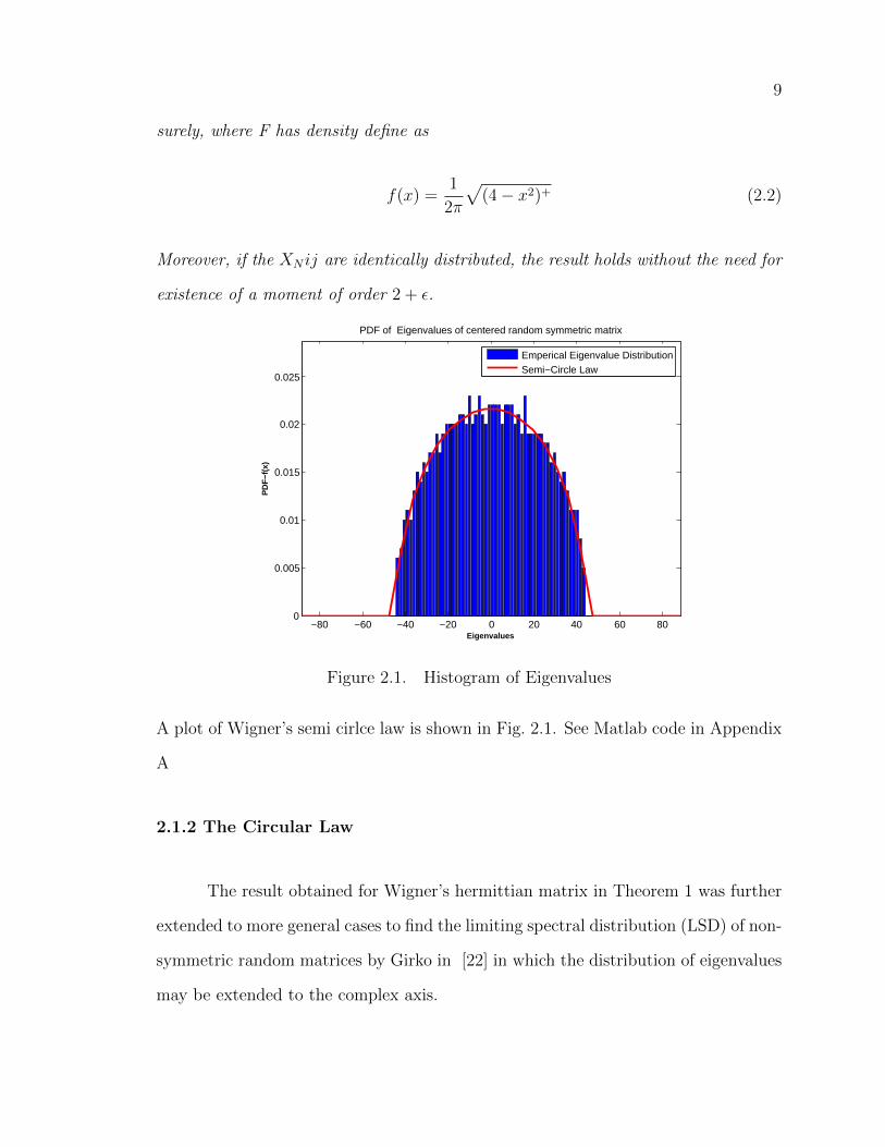
surely, where F has density define as

f(x) =1

2π

√(4− x2)+ (2.2)

Moreover, if the XN ij are identically distributed, the result holds without the need for

existence of a moment of order 2 + ε.

−80 −60 −40 −20 0 20 40 60 800

0.005

0.01

0.015

0.02

0.025

Eigenvalues

PD

F−f

(x)

PDF of Eigenvalues of centered random symmetric matrix

Emperical Eigenvalue DistributionSemi−Circle Law

Figure 2.1. Histogram of Eigenvalues

A plot of Wigner’s semi cirlce law is shown in Fig. 2.1. See Matlab code in Appendix

A

2.1.2 The Circular Law

The result obtained for Wigner’s hermittian matrix in Theorem 1 was further

extended to more general cases to find the limiting spectral distribution (LSD) of non-

symmetric random matrices by Girko in [22] in which the distribution of eigenvalues

may be extended to the complex axis.

10

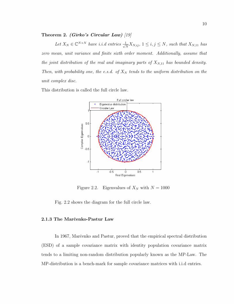
Theorem 2. (Girko’s Circular Law) [19]

Let XN ∈ CN×N have i.i.d entries 1√NXN,ij, 1 ≤ i, j ≤ N , such that XN,11 has

zero mean, unit variance and finite sixth order moment. Additionally, assume that

the joint distribution of the real and imaginary parts of XN,11 has bounded density.

Then, with probability one, the e.s.d. of XN tends to the uniform distribution on the

unit complex disc.

This distribution is called the full circle law.

Figure 2.2. Eigenvalues of XN with N = 1000

Fig. 2.2 shows the diagram for the full circle law.

2.1.3 The Marcenko-Pastur Law

In 1967, Marcenko and Pastur, proved that the empirical spectral distribution

(ESD) of a sample covariance matrix with identity population covariance matrix

tends to a limiting non-random distribution popularly known as the MP-Law. The

MP-distribution is a bench-mark for sample covariance matrices with i.i.d entries.

11

Theorem 3. (Marcenko-Pastur Law) [15] Assume a random N ×n matrix X ∈

CN×n with i.i.d entries ( 1√nXN,ij), such that XN,ij has zero mean and unit variance

and n→∞, N →∞ with Nn→ c ∈ (0,∞), the ESD of Rn = XXH converges almost

surely to a non random distribution function F(c) with density function given by:

fc(x) = (1− c−1)+δ(x) +1

2πcx

√(x− a)+(b− a)+ (2.3)

where a = (1−√c)2, b = (1−

√c)2 and δ(x) = 1{0}(x).

The proof of this theorem can be found on page 43 of [19].

0 0.5 1 1.5 2 2.5 30

0.1

0.2

0.3

0.4

0.5

0.6

0.7

0.8

0.9

1

x

f(x)

Empircal Eigenvalue DistributionMarchenko−Patur Law

Figure 2.3. The Spectral distribution of 1nXXH with X ∈ CN×n when n =

1000, N = 500 and c = N/n. The blue line is Marcenko-Pastur Law.

Fig. 2.3 gives the plot of the MP-law in Matlab. The matlab code can be found in

[23] and [24] as well as appendix A.

12

0.4 0.6 0.8 1 1.2 1.4 1.6 1.8 20

0.2

0.4

0.6

0.8

1

1.2

1.4

x

f(x)

Empircal Eigenvalue DistributionMarchenko−Patur Law

Figure 2.4. The Spectral distribution of 1nXXH with X ∈ CN×n when n =

1000, N = 100 and c = N/n. The blue line is Marcenko-Pastur Law.

2.2 RECENT RANDOM MATRIX TECHNIQUES

2.2.1 Free Probability of Random Matrices

The history of free probability can be traced to the pioneering work of voiculescu

in the 1980’s [25–27]. Voiculescu pointed out that freeness could be seen as an ana-

logue of the classical probability concept of ‘independence’ for random variables [28].

Free probability allows a means for the limiting spectral distribution (LSD) of several

rectangular matrices to be expressed in linear addition and multiplications analogous

to linear algebraic terms [28]. In page 162, [29] points out that free probability has

been applied to wireless networks to ‘extract information (where information in wire-

less networks is related to the eigenvalues of the random network)’ for simple models,

that is in cases where one of the matrices is unitarily invariant.

13

The significance of free probability lies in providing conditions to resolve the

difficulty in deducing the eigenvalue distribution of the sum or product of generic Her-

mitian Matrices A and B [19], chapter 4. The addition and multiplication formula for

non-cummutaitve algerba A in a fixed probability space (A, φ) with φ, a given linear

function, is based on the R-transform and S-transform. The algebra of Hermitian

random matrices involves a special case of (A, φ), for which the the random variables

(random matrices in this case), do not commute [19]. Taking the condition that the

entries of A and B are i.i.d, the asymptotic freeness condition of the LSD of ANBN

is not arbitrary.

The exact condition for which the LSD of A, B is a function of ANBN only

is unknown but sufficient condition for asymptotic freeness has been defined by free

probability theory. A number of theory must be examined to ascertain the conditions

for which the LSD function of random matrices can be said to be asymptotically free.

[28] points out the two ways to analyze the limit of distribution of random matrices

is through the resolvent method and the moment method. The resolvent method

represents the limiting distribution of the A and B with equations that can be solved

analytically. But this method requires specific resolution for every specific pair of

matrices p(AN , BN). The Moment method however, allows the limiting distribution of

p(AN , BN) to be calculated using combinatorial techniques. To instigate the property

of freeness, we assume AN and BN are random matrices with dimension N → ∞.

If AN and BN are independent and BN is a unitarily invariant ensemble, for which

UNYNU∗N is equivalent to YN , where UN is a unitary matrix. The following definition

as essential to determine the asymptotic freeness of AN and BN

14

Definition 1. (Haar Distribution) Let X be a random matrix with independent Gaus-

sian entries of zero mean and unit variance, the matrix U ∈ CN×N , is defined as:

U = X(XHX)−12 (2.4)

then the empirical spectral distribution of U of converges almost surely to the limiting

distribution:

FU(z) =1

2πδ(|z| − 1) (2.5)

as N →∞ The eigenvalues of a Haar matrix all lie on the complex unit circle

−1.5 −1 −0.5 0 0.5 1 1.5−1.5

−1

−0.5

0

0.5

1

1.5Haar Distribution N= 1000

Imag(X)

Rea

l(X)

Eigenvalues of XComplex Unit circle

Figure 2.5. Haar Distribution. Notice that all eigenvalues lie on the unitcircle. See Matlab code at Appendix A .1.5

Corollary 1. let {T1, ..., TK} be N ×N hermittian random matrices and {U1, ...UK}

be Haar distributed for all Tk. Assuming the eigenvalue distribution of all Tk converge

15

almost surely towards compactly supported probability distributions, then the random

matrices U1T1UH1 , ..., UKTKU

HK are asymptotically free almost as surely as N →∞

Definition 1 and corollary 1 sets suitable condition for freeness, making it conducive

to introduce the R and S transforms.

Furthermore, an N ×N matrix X can be said to be unitarily invariant if X has the

same distribution as

UXUH (2.6)

where U has been defined as a Unitary matrix. If X satisfies equation( 2.6), then it

can be decomposed as

X = UΛUH (2.7)

where Λ is the diagonal matrix equivalent of X and is U is unitary Haar matrix

Theorem 4. [30] a square random matrix X is a bi-unitarily-invariant, if it can be

decomposed as

X = UY (2.8)

where U is a Haar matrix and independent of unitarily invariant positive definite

matrix Y .

R-Transform.

Theorem 5. Let AN ∈ CN×N and BN ∈ CN×N be two random matrices. If AN and

BN are asymptotically free almost every where and have respective asymptotic eigen-

value probability distribution µA and µB, then AN +BN has an asymptotic eigenvalue

16

distribution µ, which is such that, if RA and RB are the respective R-transforms of

the l.s.d. of AN and BN

RA+B(z) = RA(z) +RB(z) (2.9)

almost surely, with RAN+BN the R-transform of the asymptotic eigenvalue distribution

of AN +BN . The distribution µ is often denoted µA+B

Listed below are the properties of the R-transform

(i) For any a > 0,

RaX(z) = aRX(az) (2.10)

(ii)

RF(a)(z) = aRF (az) (2.11)

where F is the LSD of X and RF(a)is the R-transform of the LSD F(a)

From theorem (5), a reasonable generalization can be applied to the random matrices

used in this work since they satisfy the condition for asymptotic freeness. The random

matrices used in this work are large random matrices with packet drop data entries

with dimensions up to X ∈ CN×n where N = 250, n = 400. It is convinent to say

a matrix of such size is a random matrix due to its size. It means then that several

realizations of {X1, ..., Xk} can be added together since they are asymptotically free.

S-Transform.

Theorem 6. ( [19]) Let XN ∈ CN×n and YN ∈ CN×n be two random matrices. If

XN and YN are asymptotically free almost everywhere and have respective (almost

17

sure) asymptotic eigenvalues distribution µA and µB, then XN , YN has an asymptotic

eigenvalue distribution µ, such that, if SA and SB are the respective S-transforms of

the LSD of XN and YN

SXY (z) = SX(z)SY (z) (2.12)

almost surely, with SXY the S-transform of the LSD of XN and YN

Listed below are the properties of the S-transform

(i) For any a > 0,

SaX(z) =1

aSX(z) (2.13)

(ii)

SF(a)(z) =

1

aSF (z) (2.14)

he application of both S and R transforms to this work are generalized based on the

following propositions:

Proposition 1. [31] Let the matrix Xi be a free family of R-diagonal matrices for

all 1 ≤ i ≤ L: Then,

1. Sum of free R-diagonal matrices: X1 + ...+XL =∑L

i=1Xi

2. Product of free R-diagonal matrices: X1...XL =∏L

i=1Xi

3. Power of a R-diagonal matrices:(Xi)p, i = 1, ...L for p ∈ R

are diagonal too.

From the foregoing, it can assumed X is asymptotically free and satisfies equa-

tion (2.6) for it to be R-diagonal. Then proposition 1 applies to X. Proposition 1

18

is necessary to establish the framework for operations performed on data collected in

this work in chapter 4.

2.2.2 Perturbed Sample Covariance Matrices

Given a random matrix X ∈ CN×n, and some operator φ to operate on A

φ(A), then the perturbation of A seeks to study how the effect of a perturbation on

A, given by (A + ε) affects the behavior of φ. In other words, perturbation theory

seeks to understand the relation between φ(A + ε) and φ(A). For this purpose of

this work, much interest is placed on the perturbation of random matrix XN by a

low rank diagonal matrix CN . From the foregoing we assume XN is a large random

matrix with dimension N, n and limN→∞,Nn→ c(c < 1). It has been shown that

the asymptotic distribution of XN follows MP-distribution. See equation. 2.3. If

the eigenvalues of CN lies outside the upper support of the MP-distribution given by

(1 +√c)2, then when CN perturbs XN , outliers (also called spikes) may be produced

outside the support of (1 +√c)2.

Stating this more formally, let the perturbed covariance matrix be modeled

as QN = T12NXNX

HN TN with i.i.d entries of zero-mean, variance 1/N . Assuming the

population covariance matrix is TN where TN contains some outlying eigenvalues, then

it can be shown that the empirical spectral distribution (ESD) of TN also converges

weakly to F . A key interest here is to determine whether the outlying eigenvalues in

TN produces corresponding outliers in the ESD of the sample covariance matrix. The

behavior of the largest eigenvalue distribution of QN is termed ‘fluctuation’ or BBP

phase-transition and was studied by [19,32–34]

Theorem 7. (Baik and Silverstein, 2006 [19]). Let QN = T12NXNX

HN TN , where

XN → CN×n has i.i.d. entries of zero mean, variance 1/n, and fourth order moment

19

of order O(1/n2), and TN → CN×N is diagonal given by:

TN = diag(α1, ..., α1︸ ︷︷ ︸k1

, ..., αM , ..., αM︸ ︷︷ ︸KM

, 1, ..., 1︸ ︷︷ ︸N−

∑Mi=1Ki

) (2.15)

with α1 > ... > αM > 0 for some M, C = limN N/n. Call #{j, αj > 1 +√c}. Denote

additionally λ1, ..., λN the eigenvalues of QN , ordered as λ1 ≥ λN . Then

1. for 1 ≤ j ≤M0, 1 ≤ i ≤ Kj

λk1+...+kj−1+i → αj +cαjαj−1

2. for the other eigenvalues, if c < 1,

* for M1 + 1 ≤ j ≤M , 1 ≤ i ≤ Kj λN−kj−...−kM+i → αj +cαjαj−1

* for the indexes of eigenvalues of TN inside [1−√c, 1 +

√c]

λk1+...+kM0+1 → (1 +

√(c)2

λkN−kM1+1−...−kM → (1−

√(c)2

if c > 1,

λn → (1−√c)2

λn+1 = ... = λN = 0

if c = 1,

λmin(n,N) → 0.

The implication of this theorem is that since TN has α1...αM0 eigenvalues whose values

exceed (1+√c), therefore k1+...+kM0 multiplicity eigenvalues lie outside the support

of the MP-distribution (1 +√c)2.

20

0 1 2 3 4 5 60

0.1

0.2

0.3

0.4

0.5

0.6

0.7

0.8

0.9

x

f(x)

Empircal Eigenvalue DistributionMarchenko−Patur Law

Outliers

Figure 2.6. Marcenko-Pastur Law with outliers.

Fig.2.6 illustrates this. When c is close to 1, some spikes may be hidden within the

bulk. In fig.2.6, the three spikes were observed outside the bulk because 1+√c < α1 <

α2 < α3 where α1, α2, and α3 are the extreme eigenvalues of the population covariance

matrix TN . The approximate value of αj can be calculated using theorem. 7. If the

approximate position of the jth outlier is known from the graph, then the approximate

position = αj +cαj

1−cαj . This result will be used to explain the outliers obtained in

chapter 4. Further study on the distribution of spiked eigenvalues outside the support

of the MP-distribution has been extensively studied by [35,36] and are found to follow

Tracy-Widom distribution.

The Ring Law.

Definition 2. Let the entries of the N×n matrix X be i.i.d. with zero mean variance

1/N : then, the empirical eigenvalue distribution of the singular value equivalent of X

21

converges almost surely to

fXu(z) ={ 1cπ

√1−c<|z|≤1

0 elsewhere (2.16)

as N, n→∞ with the ratio Nc≤ 1

−1.5 −1 −0.5 0 0.5 1 1.5−1.5

−1

−0.5

0

0.5

1

1.5

real(Z)

imag(Z

)

N=250, n=500, c=N/n=0.5, ρ =500, β = c =0.5, κ = β/ρ =0.001

EigenvaluesInner Unit CircleOuter Unit Circle

Figure 2.7. Distribution of Eigenvalues within the unit ring. See AppendixA .1.6 for Matlab code

Outliers outside the Ring Law. [34] in 2013 investigated the

spiked model of non-hermitian matrices, specifically for perturbed random matrices

when perturbed by F , given that the rank of F is bounded as the dimension go to

infinity and has eigenvalues out of the maximal circle of the single ring. The results of

[34] show that the macroscopic eigenvalue distribution of such matrices is governed

by the single ring theorem. This theorem is defined thus:

Definition 3. Assuming X is a random matrix and F is a perturbation matrix with

bounded rank lower than rb. Let ε > 0 be fixed and suppose that for all sufficiently

22

large n, F does not have any eigenvalues in the band z ∈ C, b + ε < |z| < b + 3ε

and has rb eigenvalues countd with multiplicity λ(F ), · · · , λrb(F ) with modulus higher

than b+ 3ε. Then, with probability tending to one, X + F has exactly rb eigenvalues

with modulus higher than b+ 3ε. Hence,

∀ i ∈ 1, · · · , rb, λi(X + F )− λi(F )→ 0 (2.17)

[34] further showed that there are no eigenvalues inside the annulus. All

outliers then, are due to perturbation by F .

−1.5 −1 −0.5 0 0.5 1 1.5−1.5

−1

−0.5

0

0.5

1

1.5

real(Z)

imag

(Z)

N=500, n=1250, c=N/n=0.4, β=c=0.4

EigenvaluesInner Unit CircleOuter Unit Circle

Figure 2.8. The Ring Law with 3 Outliers. The Outliers are due to pertur-bation by low-rank matrix F with eigenvalues outside the unit ring

23

2.2.3 Kernel Density Estimation

Kernel Density estimation is a non-parametric approach to estimate the proba-

bility density function of a random variable. Non-parametric approach implies Kernel

Density Estimation does not estimate the density function of random variables using

parameter estimations such as µ (mean) or σ2 (variance). Non-parametric density

estimation was first proposed by Fix and Hodges in 1951 and later made popular by

Silverman in 1986 [37]. However, the current Kernel form is credited to Emanuel

Parzen and Murray Rosenblatt who created it independently in 1956 [38]. Since Ker-

nel density estimation is non-parametric, it helps to represent the estimate (fh(x)) of

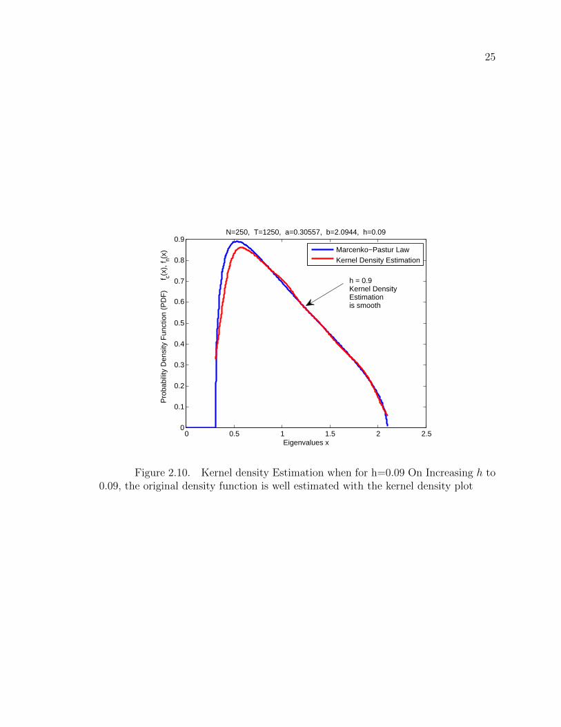
the density function (fx) of a distribution using a smoothing parameter h.

For practical purpose, a range of functions are selected as the kernel functions

e.g: normal, Epamechikov [39], triangular, biweight, triweight and others. However,

the standard normal Gaussian is usually used more often.

fh(x) =1

nh

n∑i=1

K

(x− xih

)(2.18)

The Kernel K(.) is normalized to integrate to 1 by dividing by nh. h > 0 is called

the bandwidth of the kernel function and the smaller the value of h, the higher the

sensitivity of sampling the target density function. The reverse is also true for h. It

can be shown that for fast convergence of the kernel estimator, h = n1/5 is optimum

although other values may be used if the smoothing property does not approximate

24

0 0.5 1 1.5 2 2.50

0.1

0.2

0.3

0.4

0.5

0.6

0.7

0.8

0.9

1

Eigenvalues x

Pro

babi

lity

Den

sity

Fun

ctio

n (P

DF

)

f c(x),

f n(x)

N=250, T=1250, a=0.30557, b=2.0944, h=0.02

Marcenko−Pastur LawKernel Density Estimation

h = 0.02Kernel Densityestimationis not smooth.

Figure 2.9. Kernel density Estimation when for h=0.02. Notice that thedensity function is estimated but with spurts.

the original density function as it should. Fig. 2.9 and 2.10 give examples of density

function estimation.

Summarily, some theory of random matrices given in this chapter is needed to

build a mathematical framework for results obtained in chapter 4. Howbeit, RMT is

one of the structure that framed the motivations for this work. Hence an elaborate

discussion such as the one given in this chapter is very valuable.

25

0 0.5 1 1.5 2 2.50

0.1

0.2

0.3

0.4

0.5

0.6

0.7

0.8

0.9

Eigenvalues x

Pro

babi

lity

Den

sity

Fun

ctio

n (P

DF

)

f c(x),

f n(x)

N=250, T=1250, a=0.30557, b=2.0944, h=0.09

Marcenko−Pastur LawKernel Density Estimation

h = 0.9Kernel DensityEstimationis smooth

Figure 2.10. Kernel density Estimation when for h=0.09 On Increasing h to0.09, the original density function is well estimated with the kernel density plot

CHAPTER 3

SIMULATION SETUP AND DATA COLLECTION

3.1 OPNET BASICS

Table 3.1. OPNET 17.5 Interface

In this thesis, OPNET Modeler 17.5 is used to simulate a large wireless network

and to collect data. The data collected is analyzed in Matlab. For the purpose

of familiarity, a brief overview of OPNET modeler is necessary to help build an

understanding of how the network simulation was done.

OPNET stands for Optimized Network Engineering Tools. OPNET Tech-

nologies has its headquarters at Maryland and it was co-founded by Alain Cohen

and his brother Marc in 1986. OPNET technologies was made public in 2000. In

2012, Riverbed Technologies bought OPNET at about $1 billion. OPNET tech-

nologies provide a range of software tools for managing networks and other related

26

27

services spanning application performance management, network planning, network

engineering, network operations and research and development. OPNET products for

application performance management is used for analytics of network applications.

OPNET panorama is used for real-time applications and analytics while IT Guru

Systems Planner is used for systems capacity management [40]. Simulations in OP-

NET is Descrete-Event based. It uses a Discrete Event Simulation approach to allow

interaction between events in a network to be efficiently represented. Event-based

simulations in OPNET are time based and the time is assigned by OPNET’s software

kernel while interactions between events are simulated based on the time assigned in

the simulation. OPNET modeler was the first application created by OPNET tech-

nologies. The hierarchical implementation method of network design used in OPNET

allows for a top-down design approach from the MAC layer to the Application layer

or from the Application layer to the MAC layer.

OPNET is one among a list of network simulation software packages. Popular

network simulation packages include: OPNET Modeler, NS-2, OMNeT++, the Java-

based JiST, the WSN simulator TOSSIM, Qualnet, GloMoSIM and host of others [41].

Although network simulators try to model real work network scenarios, they are not

perfect, but they give close enough result to give the researcher a meaningful insight

into the network under test [42]. Table. 3.2 was culled from page 13 of [1] and gives a

host of comparison between various popular network simulation platforms available.

To obtain further critical survey of network simulators and their relative usage

in academia, [1] surveyed all papers published in IEEE transactions (8370) on Net-

working, IEEE GLOBECOM, INFOCOM and ICC from 2007 to 2009; the conclusion

arrived at a relative distribution of the use of network simulation packages in those

papers:

28

Simulator Type Deployment

mode

Network impairments Network protocol

supported

OPNET Commercial

/academic

Enterprise Link models such as bus and point-

to-point (P2P), queuing service such

as Last-in-First-Out (LIFO), First-

in-First-Out (FIFO), priority non-

preemptive queuing, round-robin.

ATM, TCP, Fiber

distributed data interface

(FDDI), IP, Ethernet, Frame

Relay, 802.11, and support

for wireless.

QualNet Commercial Enterprise Evaluation of various protocols. Wired and wireless

networks; wide-area

networks.

NetSim Commercial

/academic

Large-scale Relative positions of stations on the

network, realistic modeling of signal

propagation, the transmission

deferral mechanisms, collision

handling and detection process.

WLAN, Ethernet, TCP/IP,

and ATM

Shunra

VE

Commercial Enterprise Latency, jitter and packet loss,

bandwidth

congestion and utilization.

Point-to-point, N-Tier, hub

and spoke, fully meshed

networks.

Ns-2 Open source Small-scale Congestion control, transport

protocols, queuing and routing

algorithms, and multicast.

TCP/IP, Multicast routing,

TCP protocols

over wired and wireless

networks.

GloMoSim Open source Large-scale Evaluation of various wireless

network protocols including channel

models, transport, and MAC

protocols.

Wireless networks.

OMNeT++ Open source Small-scale Latency, jitter, and packet losses. Wireless networks

P2P

Realm

Open source Small-scale Verify P2P network requirements,

topology management algorithm or

resource discovery.

Peer to peer (P2P)

GTNetS Open source Large-scale Packet tracing, queuing methods,

statistical methods, random number

generators.

Point-to-Point, Shared

Ethernet, Switched

Ethernet, and Wireless

links.

AKAROA Open source Small-scale Protocol evaluation. Wired and wireless

networks, Ethernet.

Table 3.2. Comparison of Popular Network Simulators.

3.2 WHY OPNET?

The choice to use OPNET in this research is based on some criteria for which

available network simulators are used in the industry. Some of these criteria are:

1. Ease of Use

2. Popularity and relevance in academia

29

Table 3.3. Simulators used in IEEE Journals and Conference Papers Pub-lished from 2007 TO 2009 [1]

SimulatorIEEETrans. onCommun.

IEEE/ACMTrans. onNetworking

IEEE/ACMIEEEGLOBECOM

IEEEINFOCOM

IEEEICC

Overall(%)

ns-2 14 57 45 39 59 42.8OPNET 6 4 8 3 17 7.6MATLAB 78 32 29 32 13 36.8QualNet - 1 5 12 3 4.2GloMoSim - 1 1 3 3 1.6OMNet++ - - 2 - 2 0.8CustomPrograms

2 5 10 11 3 6.2

Total 100% 100% 100% 100% 100%

3. Availability of Free license for research

4. Relative Optimization of System Resources

5. Closeness of result to real world scenarios

Tables. 3.2 and 3.1 show the relative performance of the network packages based on

the list of criteria considered. OPNET’s GUI is relatively easy to use and a well

documented library is also included to help modify existing packet nodes. Although

NS-2 is open source and very popular in the research industry, it is not as user-friendly

as OPNET. Also, it doesn’t have the support for as many protocols as OPNET. Given

the shortness of time for which this research was done, OPNET could be learnt within

such time constrain. This research was awarded two research licenses from Riverbed

Technologies and Scalable Networks for OPNET and Qualnet respectively. There is

no significant reason for selecting OPNET over Qualnet. Qualnet is equally a good

choice. A few of the features of OPNET may help justify its selection as the simulation

package of choice [42].

1. Fast discrete event simulation engine

30

2. Lot of component library with source code

3. Object-oriented modeling

4. Hierarchical modeling environment

5. Scalable wireless simulations support

6. 32-bit and 64-bit graphical user interface

7. Customizable wireless modeling

8. Discrete Event, Hybrid, and Analytical simulation

9. 32-bit and 64-bit parallel simulation kernel

10. Grid computing support

11. Integrated, GUI-based debugging and analysis

12. Open interface for integrating external component libraries

3.3 OPNET MODELER ENVIRONMENT

OPNET Modeler 17.5 version was used for this research. A basic introduction

of the varios operating environment is presented:

1. Node Editor

2. Process Editor

3. Project Editor

4. Packet Editor

5. Link Editor

6. Probe Editor

7. ICI Editor

However, only the node, process, project and packet editor environment are discussed

here. Further knowledge on user and advance operations in OPNET Modeler can be

found at [40,43].

31

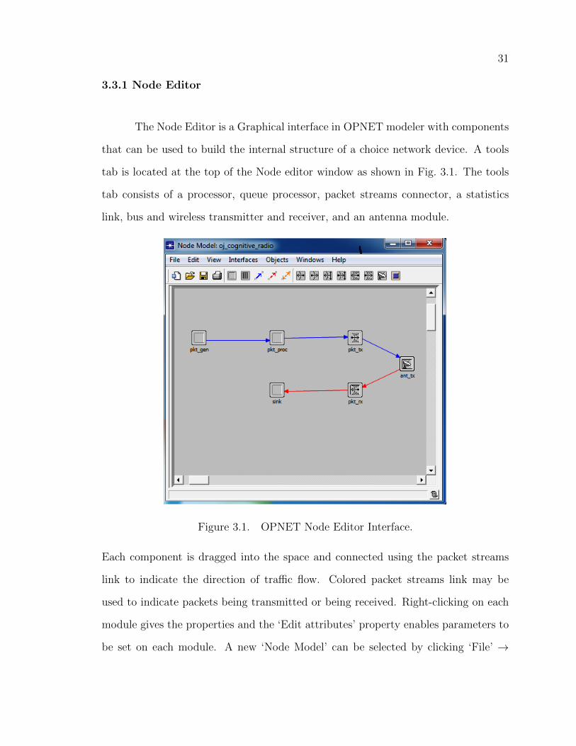
3.3.1 Node Editor

The Node Editor is a Graphical interface in OPNET modeler with components

that can be used to build the internal structure of a choice network device. A tools

tab is located at the top of the Node editor window as shown in Fig. 3.1. The tools

tab consists of a processor, queue processor, packet streams connector, a statistics

link, bus and wireless transmitter and receiver, and an antenna module.

Figure 3.1. OPNET Node Editor Interface.

Each component is dragged into the space and connected using the packet streams

link to indicate the direction of traffic flow. Colored packet streams link may be

used to indicate packets being transmitted or being received. Right-clicking on each

module gives the properties and the ‘Edit attributes’ property enables parameters to

be set on each module. A new ‘Node Model’ can be selected by clicking ‘File’ →

32

‘New’ → ‘Node Model’. One invaluable tool of assistance is OPNET documentation.

The documentation provides helps and examples to guide in using OPNET. OPNET

documentation is available from the help section of any of the editor interfaces. To

configure the working principle of each module, one may double-click on any of the

processor modules. Double-clicking any of the processor modules reveals a ‘process-

model’ in the ‘process editor’ interface.

3.3.2 Process Editor

The process editor is OPNET’s interface for customizing the operation of either

an existing node or a new one. It provides a means to write codes in C++ which can

be compiled by OPNET’s kernel using a C++ compiler. A C++ compiler must be

properly configured to work with OPNET during installation. Essentially, the process

model allows an algorithm to be implemented in the processor modules of the node

model. A node model may contain more than one processor module. For instance,

one processor module may be used for packet generation while another may be used

as a packet sink. Algorithms to be implemented in the process models can be done

logically with the aid of state transition diagrams (STD). Each state is indicated by

a green or red button.

The green state button represents a forced state while the red state button is

used for a conditional state. A force state green button indicates that the state flow

transitions to the next state unconditionally. The red state button indicates that a

condition in the state is met before the deciding on the destination state.

Each state button is connected to another by a state link. See Fig. 3.2. The

process model interface tab has the following icons: the state, the state link, the state

variable (SV), the temporary variable (TV), the Header Block (HB), the Feed Back

33

Figure 3.2. OPNET Process Editor Interface.

(FB), the Diagnostic Block (DB), the termination block (TB) and the compiler icon.

The state variable enable users to declare the data type of variables to be used in

programing various states. The TV icon enables codes for temporary variables to be

declared. Temporary variables are used for variables that change between states. The

HB specifies constants, imported C++/C Standard Template Libraries (STLs) and

transition conditions between states.

The compiler button is used to compile codes written in all the states. Fig. 3.2

shows texts in parenthesis on the state links between each state. This defines the

conditions that must be implemented while transitioning from one state to another.

The dark arrow button indicates the start of the finite state loop. Each state has an

entry and an exit interface for which codes can be included. Beneath each state is

the number of lines of codes written in the entry / the exit interface. On compiling

the process model, bugs may be indicated by the compiler. Each bug can be located

34

in the code by an error message indicating the line where an error occurred. If the

process models in each processor module compiles correctly, and all control structures

are adequately implemented, the node model can be exported to the Project Editor

for simulation. To create a new process model, one can click on ‘File’ → ‘New...’ →

‘Process Model’.

3.3.3 Project Editor

The project editor interface provides an environment for network configuration

and simulation. OPNET Modeler manages all simulation projects and scenarios. All

projects have one or more scenarios which may or may not be related. To create a new

project from OPNET’s main window, select File → New → Project and click OK.

Enter in the project name in the new Window and check Use Startup Wizard when

creating new scenarios. Click OK. An Initial Topology Window appears. Choose

create empty Scenario. In the Choose Network Window, choose Campus for a

campus network or choose between World, Enterprise, Office or Logical. In the Specify

Size window, choose the appropriate project window size. E.g., X Span = 1Km, Y

Span = 1Km.

When the project editor opens, the various tabs at the top have drop down

components that can be used in the creation of a network. Fig. ?? presents the

project editor setup windows. An important icon at the top tab is the Object Palette

35

Figure 3.3. Obeject Palette tree.

Utility icon. This icon opens the Object Palette Tree that lists all the network

device models and links by categories. Fig.3.3 shows the Object Palette Tree

3.4 SIMULATION SETUP

A new project editor environment is created in a Campus scale network size

spanning 3000 × 3000 square-meter horizontal terrain. OPNET Modeler’s Wire-

less Deployment Wizard is used to deploy clusters of 25 mobile nodes randomly

in the network span area. The node chosen for deployment is OPNET’s Cover-

age area transmitter adv. A base station is centrally located in the center of the

network using the same node model. Coverage area transmitter adv is used because

it has ‘PHY’ - attributes for modeling physical layer parameters and channel model

36

plus ‘Traffic’ - attributes for configuring packet transmit and re-transmit rate. Right-

clicking on any of the nodes shows the properties of the node. The ‘PHY’ attributes

of Coverage area transmitter adv allows the following settings to be made: Radio Link,

Transmitter and Receiver Settings and Traffic Parameters. Fig. 3.4 shows the network

topology.Network: Shadowing_and_Interference-Interference_no_shadowing [Subnet: top.Campus Network]

-1000 -500 0 500 1000 1500 2000

-1500

-1000

-500

0

500

1000

1500

2000

cluster

1

Cluster

2

Cluster

9

Cluster

3

Cluster

6

Cluster

5

Cluster

10

Cluster

4

Cluster

8

Cluster

7

Base_Station

Mobile_3

Mobile_5

Mobile_14

Mobile_24Mobile_25

Mobile_30

Mobile_34 Mobile_41

Mobile_47

Mobile_55

Mobile_57

Mobile_64

Mobile_66

Mobile_80

Mobile_84 Mobile_91

Mobile_97

Mobile_105

Mobile_107

Mobile_114

Mobile_116

Mobile_130

Mobile_132Mobile_134 Mobile_141

Mobile_147

Mobile_153

Mobile_155

Mobile_157

Mobile_164

Mobile_175

Mobile_178

Mobile_180

Mobile_182

Mobile_189

Mobile_200

Mobile_203

Mobile_205

Mobile_207

Mobile_214

Mobile_225

Mobile_230

Mobile_232Mobile_234 Mobile_241

Mobile_247

Figure 3.4. Network Topology in OPNET.

37

The network is modeled in resemblance to a campus network. The wire-

less channel is set for International Mobile Telecommunications-Advanced (IMT-

Advanced) termed ‘UMa-Los/NLoS(ITU-RM2135)’ model [44]. In a typical campus

network users usually sit in clusters or are found in the same building, which is the

motivation to set mobile users in clusters. As shown in Fig. 3.4, 10 clusters of 25

mobile nodes each are set in the campus network. Each cluster contains 25 uniformly

distributed mobile users in a 111× 111 square-meter area.

Table 3.4. Simulation Parameters for Mobile User and Base-Station ProfileRx Channel Mobile User Base StationAntenna Gain ( dBi) -1Rx Sensitivity ( dBm) -130 -200Min Frequency ( MHz) 1710 2110Bandwidth ( KHz) 22000 22000

Tx ChannelMin Frequency ( MHz) 2110 1710Bandwidth ( KHz) 22000 22000Channel Rate ( Mbps) 1 1Modulation qpsk qpskTx Power ( dBm) 26 30Shadow Fading Enabled Not Used

The parameters of the base station and mobile users are set in accordance with the

parameters shown in Table. 3.4. Additionaly, caution is taken to ensure that the rela-

tive distance of mobile nodes in the various clusters are close enough to approximate

a relative distance of mobile users from one another, but also to maintain similar

shadowing and path-loss model between mobile users.

38

3.4.1 Channel Model

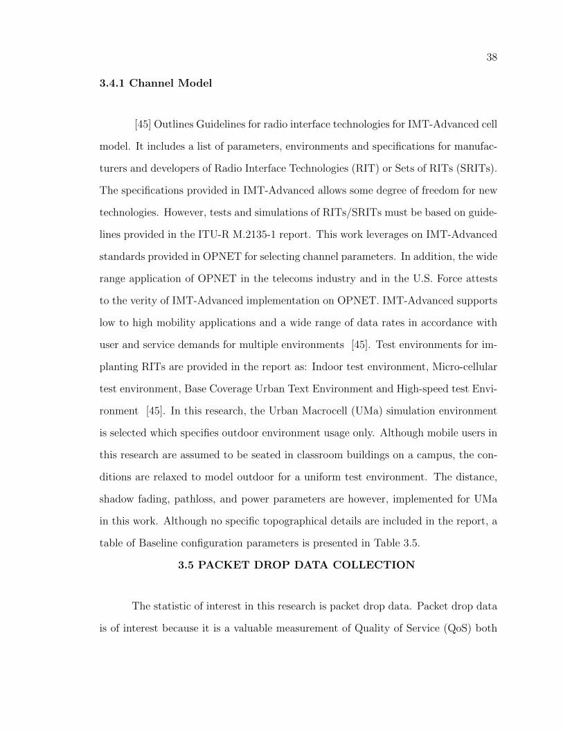
[45] Outlines Guidelines for radio interface technologies for IMT-Advanced cell

model. It includes a list of parameters, environments and specifications for manufac-

turers and developers of Radio Interface Technologies (RIT) or Sets of RITs (SRITs).

The specifications provided in IMT-Advanced allows some degree of freedom for new

technologies. However, tests and simulations of RITs/SRITs must be based on guide-

lines provided in the ITU-R M.2135-1 report. This work leverages on IMT-Advanced

standards provided in OPNET for selecting channel parameters. In addition, the wide

range application of OPNET in the telecoms industry and in the U.S. Force attests

to the verity of IMT-Advanced implementation on OPNET. IMT-Advanced supports

low to high mobility applications and a wide range of data rates in accordance with

user and service demands for multiple environments [45]. Test environments for im-

planting RITs are provided in the report as: Indoor test environment, Micro-cellular

test environment, Base Coverage Urban Text Environment and High-speed test Envi-

ronment [45]. In this research, the Urban Macrocell (UMa) simulation environment

is selected which specifies outdoor environment usage only. Although mobile users in

this research are assumed to be seated in classroom buildings on a campus, the con-

ditions are relaxed to model outdoor for a uniform test environment. The distance,

shadow fading, pathloss, and power parameters are however, implemented for UMa

in this work. Although no specific topographical details are included in the report, a

table of Baseline configuration parameters is presented in Table 3.5.

3.5 PACKET DROP DATA COLLECTION

The statistic of interest in this research is packet drop data. Packet drop data

is of interest because it is a valuable measurement of Quality of Service (QoS) both

39

Deployment

scenario for

the evaluation

process

Indoor

hotspot

Urban

micro-cell

Urban

macro-cell

Rural

macro-cell

Suburban

macro-cell

Base station (BS)

antenna

height

6 m, mounted

on ceiling

10 m, below

rooftop

25 m, above

rooftop

35 m, above

rooftop

35 m, above

rooftop

Number of BS

antenna

elements

Up to 8 rx

Up to 8 tx

Up to 8 rx

Up to 8 tx

Up to 8 rx

Up to 8 tx

Up to 8 rx

Up to 8 tx

Up to 8 rx

Up to 8 tx

Total BS transmit

power

24 dBm for

40 MHz,

21 dBm for

20 MHz

41 dBm for

10 MHz,

44 dBm for

20 MHz

46 dBm for

10 MHz,

49 dBm for

20 MHz

46 dBm for

10 MHz,

49 dBm for

20 MHz

46 dBm

for 10 MHz,

49 dBm

for 20 MHz

User terminal (UT)

power

class

21 dBm 24 dBm 24 dBm 24 dBm 24 dBm

UT antenna system Upto 2 tx

Upto 2 tx

Upto 2 tx

Upto 2 tx

Upto 2 tx

Upto 2 tx

Upto 2 tx

Upto 2 tx

Upto 2 tx

Upto 2 tx

Minimum distance

between UT and

serving cell

>= 3 m >= 10 m >= 25 m >= 35 m >= 35 m

Carrier frequency

(CF) for evaluation

(representative of

IMT bands)

3.4 GHz 2.5 GHz 2 GHz 800 MHz Same as urban

macro-cell

Outdoor to indoor

building

penetration loss

N.A. - N.A. N.A. 20 dB

Outdoor to in-car

penetration loss

N.A. N.A. 9 dB (LN, 𝜎 =5 dB)

9 dB (LN,

𝜎 = 5 dB)

9 dB (LN, 𝜎 =5 dB)

Table 3.5. Baseline configurations for IMT-Advanced.

in wireless sensor networks, and in ad-hoc mobile networks. Packet drops can easily

be collected at low overhead from individual nodes. Yet, it does not reveal sensitive

information about the content of the packet, it only measures discrete values of packet

losses per individual nodes. Packet drops in a wireless network may be caused by a

combination of factors, some of which may include: relative distance of receiver from

the transmitter, pathloss model of the channel, hardware variation between sending

40

and receiving pairs, differences in receiver sensitivity and oscillator calibration [46].

To record significant packets received at each mobile nodes, the base station is made

Figure 3.5. Discrete Event Simulation Parameters for the Topology used inthis work

to transmit packets at 20 packets/seconds. The size of each packet is set to a uniform

1024 bits for a conservative case. To select the simulation statistic to packet drops,

right-click on the open space in the project editor, click Choose Individual DES

Statistics. In the Choose Results window, select Received Packets Dropped.

Click Ok and save changes. The simulation is made to run for 400 seconds. It must be

noted here that OPNET uses Discrete-Events-Simulation (DES) to run simulations

between configured events. OPNET Modeler’s DES is set to the parameters shown

in Fig.3.5. The simulation is executed for three scenarios:

1. Shadowing enabled in the network

2. One Jammer is placed in the network

3. Four Jammers are placed in the network

41

After the simulation completes, the Received Packets Dropped statistic is

displayed for all 250 nodes in the results viewer graph. The packet drop graph for

each node is superimposed on one another for all 250 nodes. When superimposing

packet drop data, it was observed that clusters closer to the base-station had a lower

mean packet drop value and a lower packet drop range, while clusters farther away

had a higher average packet drop and a higher variance in packet drop values. Fig. 3.6

shows packet drop signature for selected nodes in the network.

OPNET provides a feature for exporting graphs to Microsoft Excel. All the

statistic superimposed in the results viewer graph are exported to spreadsheet and

saved. This is repeated for all the scenarios mentioned in section( 3.5).

3.5.1 Shadowing enabled in the network

By enabling shadowing in the network, OPNET simulates a wireless network

environment similar to IMT-advanced standard for shadow fading in an Urban Macro-

cell. [47] Describes shadow fading for IMT. Shadow fading is modeled independently

per base station site as:

PLinst = PL+ Zi (3.1)

where PLinst is instantaneous pathloss, PL is the pathloss and Zi is the ordinary

shadow random variable [47]. For various Base-stations to Mobile user, Zi must be

calculated separately. Essentially, shadow fading varies exponentially with distance

between two mobile users with same transmitting base station. When shadowing is

enabled, all nodes implement IMT shadowing fading standard in OPNET. To begin

42

data collection, the simulation is made to run for 400 seconds as described in sec-

tion( 3.4). Fig. 3.6 Shows Received Packet Dropped when shadowing was enabled

on the network.

Figure 3.6. Packet Drop Signature for selected nodes in all 10 clusters whenShadowing is enabled in the network

43

Network: Shadowing_and_Interference-Interference_jamming_100W_20percent [Subnet: top.Campus Network]

-1000 -500 0 500 1000 1500 2000

-1500

-1000

-500

0

500

1000

1500

2000

cluster

1

Cluster

2

Cluster

9

Cluster

3

Cluster

6

Cluster

5

Cluster

10

Cluster

4

Cluster

8

Cluster

7

Jammer

Base_Station

Jammer

Mobile_3

Mobile_5

Mobile_14

Mobile_24

Mobile_30

Mobile_37

Mobile_39

Mobile_49Mobile_50

Mobile_55

Mobile_62

Mobile_64

Mobile_74Mobile_75

Mobile_80

Mobile_84 Mobile_91

Mobile_97

Mobile_105

Mobile_114

Mobile_116Mobile_124

Mobile_130

Mobile_139

Mobile_141Mobile_149

Mobile_155

Mobile_164

Mobile_166Mobile_174

Mobile_182

Mobile_189

Mobile_191

Mobile_205

Mobile_214

Mobile_216Mobile_224

Mobile_230

Mobile_239

Mobile_241Mobile_249

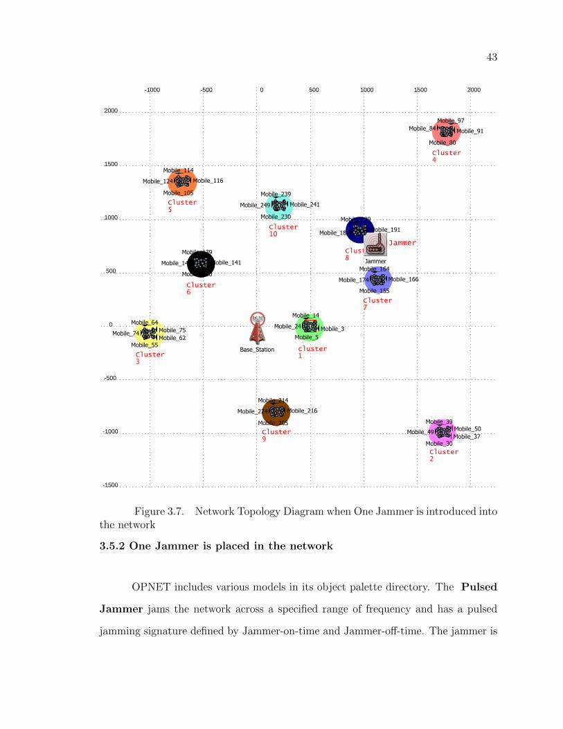
Figure 3.7. Network Topology Diagram when One Jammer is introduced intothe network

3.5.2 One Jammer is placed in the network

OPNET includes various models in its object palette directory. The Pulsed

Jammer jams the network across a specified range of frequency and has a pulsed

jamming signature defined by Jammer-on-time and Jammer-off-time. The jammer is

44

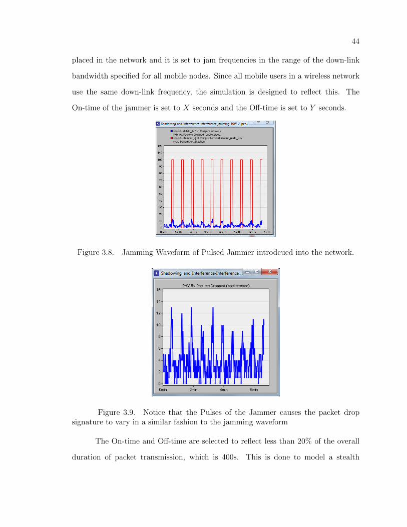
placed in the network and it is set to jam frequencies in the range of the down-link

bandwidth specified for all mobile nodes. Since all mobile users in a wireless network

use the same down-link frequency, the simulation is designed to reflect this. The

On-time of the jammer is set to X seconds and the Off-time is set to Y seconds.

Figure 3.8. Jamming Waveform of Pulsed Jammer introdcued into the network.

Figure 3.9. Notice that the Pulses of the Jammer causes the packet dropsignature to vary in a similar fashion to the jamming waveform

The On-time and Off-time are selected to reflect less than 20% of the overall

duration of packet transmission, which is 400s. This is done to model a stealth

45

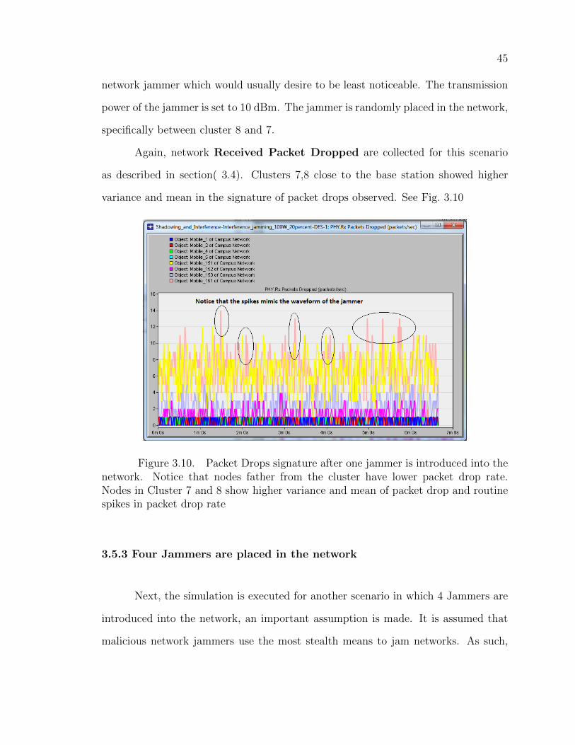
network jammer which would usually desire to be least noticeable. The transmission

power of the jammer is set to 10 dBm. The jammer is randomly placed in the network,

specifically between cluster 8 and 7.

Again, network Received Packet Dropped are collected for this scenario

as described in section( 3.4). Clusters 7,8 close to the base station showed higher

variance and mean in the signature of packet drops observed. See Fig. 3.10

Figure 3.10. Packet Drops signature after one jammer is introduced into thenetwork. Notice that nodes father from the cluster have lower packet drop rate.Nodes in Cluster 7 and 8 show higher variance and mean of packet drop and routinespikes in packet drop rate

3.5.3 Four Jammers are placed in the network

Next, the simulation is executed for another scenario in which 4 Jammers are

introduced into the network, an important assumption is made. It is assumed that

malicious network jammers use the most stealth means to jam networks. As such,

46

we assume that they use various jamming devices or at least the jamming waveform

signal is not exactly the same from jammer to jammer. Since the waveform of the

jamming signal can vary considerably from one to another, a combination of various

random distributions for the on-time and off-time of the jamming waveform is used.

To introduce such various distributions into the on-time and off-time attribute of

OPNET’s Pulsed jammer node, the process model of the pulsed jammer is modified.

Figure 3.11. Modified Process Model of OPNET’s Pulsed Jammer

Fig. 3.11 shows the modified process model of the pulsed jammer. At the init

state, all variables are initialized after which the condition statement BEGSIM is

executed. This allows the state transition to the wait for the first packet state.

The four Jammers are named individually and set to different distribution profiles as

described in section. 3.5.3. Table. 3.6 gives the distribution profile of on-off time of

each jammer introduced into the network.

Jammer1 has a mean Off-time of 50s with a standard deviation of 20s. Its

On-time profile has a mean on-time of 10s and a standard deviation of 10s.

47

Table 3.6. Simulation Parameters for jammer’s profile used in OPNET (µ =mean, σ = standard deviation)

On/OFF Time Jammer 1 Jammer 2 Jammer 3 Jammer 4

Off-Time(s)Normal Dist.µ = 50σ = 20

Constant70

Exponential Distµ = 45

Poisson Dist.µ = 70

On-Time(s)Normal Dist.µ = 10σ = 10

Constant4

Uniform Dist.Min=5Max=20

Uniform Dist.Min=7Max=30

Figure 3.12. Pulsed Waveform of Jammer1 and corresponding packet drop profile

Jammer2 is set to a constant 70s off-time and a constant on-time of 4 seconds.

Jammer3 is set to an exponential off-time of mean = 45s, and an on-time with uniform

distribution, min=5s, max=20s

Lastly, jammer4 is set to have an Off-time that is exponentially distributed with

mean=70s and an On-time with uniform distribution in the range: min=7s, max=30s.

All four jammers are then randomly placed in the network as shown in Fig. 3.16

The exported result in spreadsheet is analyzed using RMT tools in chapter 4.

48

Figure 3.13. Pulsed Waveform of Jammer2 and corresponding packet drop profile

Figure 3.14. Pulsed Waveform of Jammer3 and corresponding packet drop profile

Figure 3.15. Pulsed Waveform of Jammer4 and corresponding packet drop profile

49

Network: Shadowing_and_Interference-Interference_4_jammers_10W [Subnet: top.Campus Network]

-1000 -500 0 500 1000 1500 2000

-1500

-1000

-500

0

500

1000

1500

2000

cluster

1

Cluster

2

Cluster

9

Cluster

3

Cluster

6

Cluster

5

Cluster

10

Cluster

4

Cluster

8

Cluster

7

Base_Station

Mobile_16

Mobile_22

Mobile_24

Mobile_30

Mobile_39

Mobile_49Mobile_50

Mobile_57

Mobile_64

Mobile_80

Mobile_89

Mobile_91Mobile_99

Mobile_105

Mobile_109

Mobile_122

Mobile_130

Mobile_139

Mobile_141Mobile_149

Mobile_155

Mobile_159 Mobile_166

Mobile_172

Mobile_180

Mobile_189

Mobile_199

Mobile_205

Mobile_214

Mobile_216Mobile_224

Mobile_230

Mobile_239

Mobile_241

Jammer_Const_Const

Jammer_EXP_UNFRM

POI_UNIF

Jammer_NRM_NRM

Figure 3.16. Network Topology with 4 Jammers Introduced

CHAPTER 4

DATA ANALYSIS BY CASE STUDIES

4.1 INTRODUCTION

Chapter 2 has dealt sufficient introduction to the theoretical tools that can be

used to analyze the large packet drop matrices collected in chapter 3. In chapter 1

it was mentioned that this work is motivated by the application of Random matrix

theory to Big-Data as a framework for Large Network data analysis. As such, the

analysis of data in this work is carried out with Random Matrix theory tools presented

in chapter 2 from an Big-Data perspective. The data used in this work may not count

for Big-Data in scale but Big-Data perception is presented from the angle that the

packet drop matrices are large random matrices: XN ∈ CN×n with N, n → ∞ as

N/n→ c (c < 1).

Essentially then, it can be shown that if XN is large enough (with dimensions

N, n → ∞), with non-zero i.i.d entries, it can be counted as a random matrix and

can be treated as such. Although the packet drop matrices used in this work has

dimension N = 250 × n = 400, it is large enough to be treated as a random matrix

and the results obtained here can be extended to XN with N, n→∞ no matter the

size of N, n as long as they tend to infinity. This argument can be extended to Big-

Data as long as the data can be modeled into a large random matrix. Summarily, the

results obtained in the work can be extended to a very large network if the conditions

of random matrix theory are followed by the data collected in that network as in this

work.

50

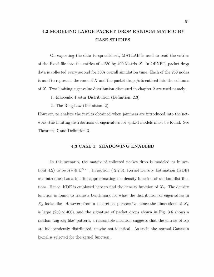
51

4.2 MODELING LARGE PACKET DROP RANDOM MATRIC BY

CASE STUDIES

On exporting the data to spreadsheet, MATLAB is used to read the entries

of the Excel file into the entries of a 250 by 400 Matrix X. In OPNET, packet drop

data is collected every second for 400s overall simulation time. Each of the 250 nodes

is used to represent the rows of X and the packet drops/s is entered into the columns

of X. Two limiting eigenvalue distribution discussed in chapter 2 are used namely:

1. Marcenko Pastur Distribution (Definition. 2.3)

2. The Ring Law (Definition. 2)

However, to analyze the results obtained when jammers are introduced into the net-

work, the limiting distributions of eigenvalues for spiked models must be found. See

Theorem 7 and Definition 3

4.3 CASE 1: SHADOWING ENABLED

In this scenario, the matrix of collected packet drop is modeled as in sec-

tion( 4.2) to be XS ∈ CN×n. In section ( 2.2.3), Kernel Density Estimation (KDE)

was introduced as a tool for approximating the density function of random distribu-

tions. Hence, KDE is employed here to find the density function of XS. The density

function is found to frame a benchmark for what the distribution of eigenvalues in

XS looks like. However, from a theoretical perspective, since the dimensions of XS

is large (250 × 400), and the signature of packet drops shown in Fig. 3.6 shows a

random ‘zig-zag-like’ pattern, a reasonable intuition suggests that the entries of XS

are independently distributed, maybe not identical. As such, the normal Gaussian

kernel is selected for the kernel function.

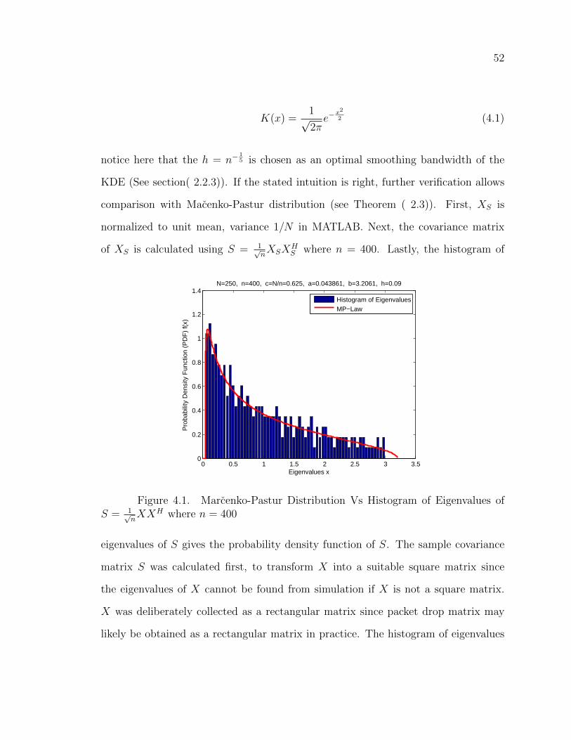
52

K(x) =1√2πe−

x2

2 (4.1)

notice here that the h = n−15 is chosen as an optimal smoothing bandwidth of the

KDE (See section( 2.2.3)). If the stated intuition is right, further verification allows

comparison with Macenko-Pastur distribution (see Theorem ( 2.3)). First, XS is

normalized to unit mean, variance 1/N in MATLAB. Next, the covariance matrix

of XS is calculated using S = 1√nXSX

HS where n = 400. Lastly, the histogram of

0 0.5 1 1.5 2 2.5 3 3.50

0.2

0.4

0.6

0.8

1

1.2

1.4

Eigenvalues x

Pro

babi

lity

Den

sity

Fun

ctio

n (P

DF

) f(

x)

N=250, n=400, c=N/n=0.625, a=0.043861, b=3.2061, h=0.09

Histogram of EigenvaluesMP−Law

Figure 4.1. Marcenko-Pastur Distribution Vs Histogram of Eigenvalues ofS = 1√

nXXH where n = 400

eigenvalues of S gives the probability density function of S. The sample covariance

matrix S was calculated first, to transform X into a suitable square matrix since

the eigenvalues of X cannot be found from simulation if X is not a square matrix.

X was deliberately collected as a rectangular matrix since packet drop matrix may

likely be obtained as a rectangular matrix in practice. The histogram of eigenvalues

53

of S is plotted against MP-distribution for comparison. See Fig. 4.1. KDE is used to

estimate the density function of S and plotted against MP-law for a closer comparison.

See Fig. 4.2.

0 0.5 1 1.5 2 2.5 3 3.50

0.2

0.4

0.6

0.8

1

1.2

1.4

Eigenvalues x

Pro

babi

lity

Den

sity

Fun

ctio

n (P

DF

)

f c(x),

f n(x)

N=250, n=400, c=N/n=0.625, a=0.043861, b=3.2061, h=0.09

Marcenko−Pastur LawKernel Density Estimation

Figure 4.2. Marcenko-Pastur Distribution Vs KDE of the spectral distribu-tion of S = 1√

nXSX

HS where n = 400

As seen in 4.2, the KDE of the sample covariance matrix of X approximates

to the MP-Law, which implies that the entries of XS are independently distributed.

This result forms an important benchmark to study the variation on the probability

density function (pdf) of XS in the following case studies.

In addition, the ring law (see section ( 2.2.2)) can be used to provide an anal-

ogous comparison between the limiting spectral properties of XS within the unit ring

and the limiting spectral distribution of a random matrix X ∈ CN×n with conditions

satisfying Definition ( 2). Already Fig.( 2.6) shows that the distribution of XN is uni-

form within the unit ring. As such, like the case of the MP-distribution, a comparison

is made between the spectral distribution of Xs and X.

54

−1.5 −1 −0.5 0 0.5 1 1.5−1.5

−1

−0.5

0

0.5

1

1.5

real(Z)

imag

(Z)

N=250, n=400, c=N/n=0.625, β=c=0.625

EigenvaluesInner Unit CircleOuter Unit Circle

Figure 4.3. The Spectral Distribution of Xs within the unit ring

4.3.1 Case 1 - Discussion

The result of Fig. 4.1, 4.2 and 4.3 comply with Theorem 3 and Definition 2

for the spectral distribution of a random matrix X ∈ CN×n when the dimensions of

N, n→∞ and N/n→ c(c < 1). c = 0.625 in this case. Since the spectral distribution

follows MP-distribution, it can be concluded that shadow fading has no significant

effect on the spectral distribution of packet drop data collected in a large network. To

make this convenient conclusion, shadow fading is disabled on all the nodes and the

spectral distribution is plotted against MP-distribution. (see Fig.4.3.1) and a nearly

perfect match between both plots is obtained. Furthermore, a significant explanation

for the indifference in spectral distribution when shadow fading is enabled or disabled

is because the effect of shadowing on packet drop is an increase in variance and mean

of packet drops from the affected nodes. But the signature of packet drop data is still

55

random even when the variance and mean increases. On normalization of the data,

there is no dominant mode created in the rows of XS due to shadowing. Hence, the

entries of XS is still independent and obeys MP-distribution.

0 0.5 1 1.5 2 2.5 3 3.50

0.2

0.4

0.6

0.8

1

1.2

1.4

Eigenvalues x

Pro

babi

lity

Den

sity

Fun

ctio

n (P

DF

) f(

x)

N=250, n=400, c=N/n=0.625, a=0.043861, b=3.2061, h=0.09

Histogram of EigenvaluesMP−Law

(a) MP-law vs histogram of eigenvalues

when shadowing is disabled

0 0.5 1 1.5 2 2.5 3 3.50

0.2

0.4

0.6

0.8

1

1.2

1.4

Eigenvalues x

Pro

babi

lity

Den

sity

Fun

ctio

n (P

DF

) f(

x)

N=250, n=400, c=N/n=0.625, a=0.043861, b=3.2061, h=0.09

Histogram of EigenvaluesMP−Law

(b) MP-law vs histogram of eigenvalues

when shadowing is enabled

Figure 4.4. Comparison of Eigenvalue distribution when shadowing is dis-abled and when shadowing is enabled in the network. Notice that there is notsignificant difference

4.4 CASE 2: ONE JAMMER IS PLACED IN THE NETWORK

In this case study, the network simulation is modeled as explained in section

( 3.5.2). Packet drop traffic is also collected and modeled into XJ1 as shown in section

( 4.2). The spectral distribution of XJ1 is obtained by simulation as in section ( 4.3).

To compare the histogram of eigenvalues of XJ1 to the marcenko-pastur limiting

distribution, a plot of both is made on same graph in Fig.4.5. Additionally. the

spectral distribution of XJ1 can be rightly approximated using KDE. Hence, a similar

comparison to Fig.4.2 is made by plotting the KDE of the spectral distribution of XJ1

and the MP-distribution. see Fig.4.6.In Fig.4.5, one eigenvalue spike is produced which reflects an extreme eigenvalue in

the spectral values of XJ1. Since a spike is observed, Theorem 7 presents a suitable

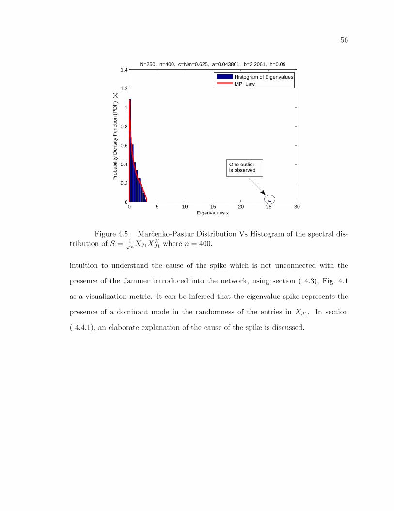
56

0 5 10 15 20 25 300

0.2

0.4

0.6

0.8

1

1.2

1.4

Eigenvalues x

Pro

babi

lity

Den

sity

Fun

ctio

n (P

DF

) f(

x)

N=250, n=400, c=N/n=0.625, a=0.043861, b=3.2061, h=0.09

Histogram of EigenvaluesMP−Law

One outlier is observed

Figure 4.5. Marcenko-Pastur Distribution Vs Histogram of the spectral dis-tribution of S = 1√

nXJ1X

HJ1 where n = 400.

intuition to understand the cause of the spike which is not unconnected with the

presence of the Jammer introduced into the network, using section ( 4.3), Fig. 4.1

as a visualization metric. It can be inferred that the eigenvalue spike represents the

presence of a dominant mode in the randomness of the entries in XJ1. In section

( 4.4.1), an elaborate explanation of the cause of the spike is discussed.

57

0 0.5 1 1.5 2 2.5 3 3.50

0.2

0.4

0.6

0.8

1

1.2

1.4

Eigenvalues x

Pro

babi

lity

Den

sity

Fun

ctio

n (P

DF

)

f c(x),

f n(x)

N=250, n=400, c=N/n=0.625, a=0.043861, b=3.2061, h=0.09

Marcenko−Pastur LawKernel Density Estimation

A minor deviation frommarcenko−pastur law

Figure 4.6. Marcenko-Pastur Distribution Vs KDE of the spectral distribu-tion of S = 1√

nXJ1X

HJ1 where n = 400

Fig. 4.6 shows that the entries of XJ1 are independent since the kernel approximation

of eigenvalues only deviate slightly from the MP-distribution. XJ1 can be said to

converge weakly to the MP-distribution.

4.4.1 Case 2 - Discussion

Couillet and Debbah in page 224 of [19] models the presence of spiked eigen-

values in a covariance matrix as QN = T12NXNX

HN TN (see section( 2.2.2)) with non-

negative eigenvalues {α1 · · ·αM} outside the Mp-law support and another set of

eigenvalues {τ1 · · · τN} within the support of {1 −√c, 1 +

√c}. The cause of the

presence of eigenvalues spikes in the limiting spectral distribution of XN are due to

{α1 · · ·αM}. In this case study, one eigenvalue spike αi, 1 ≤ i ≤ M was observed

in the spectral histogram of S = 1√nXJ1X

HJ1 (see Fig. 4.5). The majority of eigen-

bulk follow MP-distribution while the eigenspike is located at a considerable distance

58

−1.5 −1 −0.5 0 0.5 1 1.5−1.5

−1

−0.5

0

0.5

1

1.5

real(Z)

imag

(Z)

N=250, n=400, c=N/n=0.625, β=c=0.625

EigenvaluesInner Unit CircleOuter Unit Circle

One outlier

Inner circle shrinks towards the center

Figure 4.7. The Spectral Distribution of XJ1 within the unit ring. Noticethat the inner ring shrinks towards the center of the circle and the bulk of eigenvaluesalso shift likewise compared to the unit ring in Fig. 4.3

from the bulk. If the samples used were base-band samples, [19] explained that the

presence of eigenvalue spike indicates the presence of signal. However, since the data

collected in this work is packet drop data, the presence of the eigenvalue spike in

Fig. 4.5 is due to some correlation introduced into the packet drop data values of

nodes affected by the jammer. The effect of introducing the jammer into the network

(see section ( 3.5.2)) as an anonymous interference causes packet drop data, although

random on large scale, to take the waveform signature of the jamming signal.

Hence, on a large scale, the nodes affected by the jammer show a dominating

pattern in their packet drop metric corresponding to the on-time, off-time pattern

of the jammer. Essentially, when the jammer is off, packet drop data values vary

with collective mean and variance of nodes in the same cluster. When the jammer

comes on, packet drop data increases suddenly, and the instantaneous of packet drop

due to the jammer depends on the relative distance of the node from the jammer.

59

Fig. 3.9 illustrates the effect of the jammer on packet drop data of affected nodes. In

addition, αi, 1 ≤ i ≤ M refers to the eigenvalue of the true population matrix TN ;

assuming TN is a diagonal matrix with a value > 1 +√c. From Theorem 7, Baik

and Silverstein showed that the index position of the eigenvalue spike observed in

the support of the MP-distribution 1 −√c, 1 +

√c is at αj +

cαjαj−1 . Since the index

position of the eigenvalue spike in Fig. 4.5 can be obtained from simulation, α1 can

be calculated from a simple quadratic equation.

Spiked Model for Packet Drop Data with One Anonymous Interfer-

ence. Additionally, Fig. 4.8 gives one outlier unlike section( 4.3), Fig. 4.3.

To understand if the presence of an outlier outside the ring in Fig. 4.8 is related to the

eigenvalue spike observed in Fig. 4.5, an investigation of the results in Definition ( 3)

[34] show that an outlier is observed in the annulus when a random matrix XN satis-

fying the definition, with i.i.d entries is perturbed by a bounded finite rank matrix F

with rank ≤ rb and rb eigenvalues outside the bounds of {z ∈ C, b+ ε < |z| < b+ 3ε}.

If j < rb are the eigenvalues with modulus greater than b + 3ε, then, with near 1

probability, X +F has j eigenvalues greater than {b+ 3ε}. In referring to the packet

drop matrix collected in this scenario (XJ1), since one outlier was observed, the result

of [34] shows that XJ1 can be modeled as the result of a perturbed random matrix

X with another perturbation matrix F .

From the foregoing, the original matrix obtain in the shadowing scenario (XS)

could be conveniently taken as the perturbed random matrix. While F could be

modeled as a rank-1 matrix with one eigenvalue satisfying the condition of Definition

( 3). Modeling F as a rank-1 matrix is good enough since only one outlier was

observed. Also, if there are other outliers which are < {b + ε}, i.e within the inner

ring, [34] has further shown that they are not shown in the plot of the ring-law.

60

In other words, there are no eigenvalues within the inner-ring of the ring-law. It is

convenient then, to write an approximate model equation for the packet drop data

when one jammer is involved as:

0 5 10 15 20 250

0.2

0.4

0.6

0.8

1

1.2

1.4

Eigenvalues x

Pro

babi

lity

Den

sity

Fun

ctio

n (P

DF

) f(

x)

N=250, n=400, c=N/n=0.625, a=0.043861, b=3.2061, h=0.13572

Histogram of EigenvaluesMP−Law

Outlier obtained using model equation

Figure 4.8. Reproducing Fig. 4.5 using equation ( 4.2)

XJ1 = XS + F (4.2)

where XS is the packet drop matrix when shadowing is enabled/disabled in the net-

work, XJ1 is the packet drop matrix when one jammer is placed in the network and F

is perturbation matrix due to Jammer. It must be noted however, the equation( 4.2)

does not take into account the correlation introduced into XJ1 due to the effect of

jammer on packet drop, but the correlation effect is assumed negligible since the spec-

tral distribution of eigenvalues still converge weakly to MP-distribution. The model

equation was confirmed by simulation in MATLAB, using a different random matrix

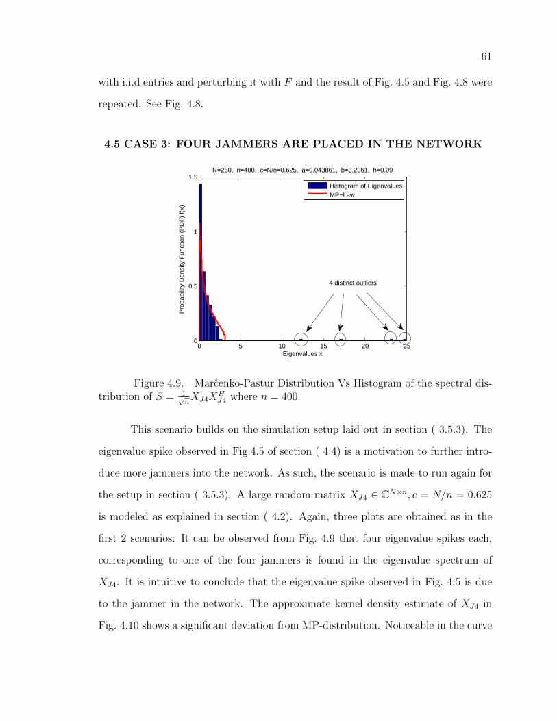
61

with i.i.d entries and perturbing it with F and the result of Fig. 4.5 and Fig. 4.8 were

repeated. See Fig. 4.8.

4.5 CASE 3: FOUR JAMMERS ARE PLACED IN THE NETWORK

0 5 10 15 20 250

0.5

1

1.5

Eigenvalues x

Pro

babi

lity

Den

sity

Fun

ctio

n (P

DF

) f(

x)

N=250, n=400, c=N/n=0.625, a=0.043861, b=3.2061, h=0.09

Histogram of EigenvaluesMP−Law

4 distinct outliers

Figure 4.9. Marcenko-Pastur Distribution Vs Histogram of the spectral dis-tribution of S = 1√

nXJ4X

HJ4 where n = 400.

This scenario builds on the simulation setup laid out in section ( 3.5.3). The

eigenvalue spike observed in Fig.4.5 of section ( 4.4) is a motivation to further intro-

duce more jammers into the network. As such, the scenario is made to run again for

the setup in section ( 3.5.3). A large random matrix XJ4 ∈ CN×n, c = N/n = 0.625

is modeled as explained in section ( 4.2). Again, three plots are obtained as in the

first 2 scenarios: It can be observed from Fig. 4.9 that four eigenvalue spikes each,

corresponding to one of the four jammers is found in the eigenvalue spectrum of

XJ4. It is intuitive to conclude that the eigenvalue spike observed in Fig. 4.5 is due

to the jammer in the network. The approximate kernel density estimate of XJ4 in

Fig. 4.10 shows a significant deviation from MP-distribution. Noticeable in the curve

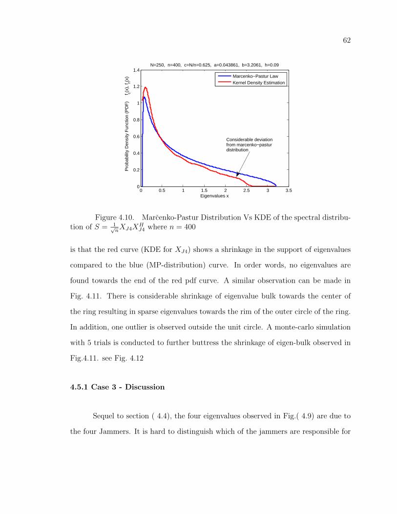
62

0 0.5 1 1.5 2 2.5 3 3.50

0.2

0.4

0.6

0.8

1

1.2

1.4

Eigenvalues x

Pro

babi

lity

Den

sity

Fun

ctio

n (P

DF

)

f c(x),

f n(x)

N=250, n=400, c=N/n=0.625, a=0.043861, b=3.2061, h=0.09

Marcenko−Pastur LawKernel Density Estimation

Considerable deviationfrom marcenko−pasturdistribution

Figure 4.10. Marcenko-Pastur Distribution Vs KDE of the spectral distribu-tion of S = 1√

nXJ4X

HJ4 where n = 400

is that the red curve (KDE for XJ4) shows a shrinkage in the support of eigenvalues

compared to the blue (MP-distribution) curve. In order words, no eigenvalues are

found towards the end of the red pdf curve. A similar observation can be made in

Fig. 4.11. There is considerable shrinkage of eigenvalue bulk towards the center of

the ring resulting in sparse eigenvalues towards the rim of the outer circle of the ring.

In addition, one outlier is observed outside the unit circle. A monte-carlo simulation

with 5 trials is conducted to further buttress the shrinkage of eigen-bulk observed in

Fig.4.11. see Fig. 4.12

4.5.1 Case 3 - Discussion

Sequel to section ( 4.4), the four eigenvalues observed in Fig.( 4.9) are due to

the four Jammers. It is hard to distinguish which of the jammers are responsible for

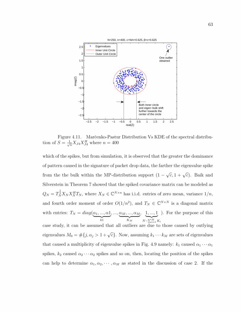
63

−2.5 −2 −1.5 −1 −0.5 0 0.5 1 1.5 2 2.5

−2.5

−2

−1.5

−1

−0.5

0

0.5

1

1.5

2

2.5

real(Z)

imag

(Z)

N=250, n=400, c=N/n=0.625, β=c=0.625

EigenvaluesInner Unit CircleOuter Unit Circle

Both Inner circle and eigen−bulk shiftfurther towards the center of the circle

One outlierobtained

Figure 4.11. Marcenko-Pastur Distribution Vs KDE of the spectral distribu-tion of S = 1√

nXJ4X

HJ4 where n = 400

which of the spikes, but from simulation, it is observed that the greater the dominance

of pattern caused in the signature of packet drop data, the farther the eigenvalue spike

from the the bulk within the MP-distribution support (1 −√c, 1 +

√c). Baik and

Silverstein in Theorem 7 showed that the spiked covariance matrix can be modeled as

QN = T12NXNX

HN TN , where XN ∈ CN×n has i.i.d. entries of zero mean, variance 1/n,

and fourth order moment of order O(1/n2), and TN ∈ CN×N is a diagonal matrix

with entries: TN = diag(α1, ..., α1︸ ︷︷ ︸k1

, ..., αM , ..., αM︸ ︷︷ ︸KM

, 1, ..., 1︸ ︷︷ ︸N−

∑Mi=1Ki

). For the purpose of this

case study, it can be assumed that all outliers are due to those caused by outlying

eigenvalues M0 = #{j, αj > 1 +√c}. Now, assuming k1 · · · kM are sets of eigenvalues

that caused a multiplicity of eigenvalue spikes in Fig. 4.9 namely: k1 caused α1 · · ·α1

spikes, k2 caused α2 · · ·α2 spikes and so on, then, locating the position of the spikes

can help to determine α1, α2, · · · , αM as stated in the discussion of case 2. If the

64

−2.5 −2 −1.5 −1 −0.5 0 0.5 1 1.5 2 2.5

−2.5

−2

−1.5

−1

−0.5

0

0.5

1

1.5

2

2.5

real(Z)

imag

(Z)

N=250, n=400, c=N/n=0.625, β=c=0.625, Monte−Carlo Tries =5

EigenvaluesInner Unit CircleOuter Unit Circle

Outliers occuralmost at thesame spot

Figure 4.12. 5 Monte-carlo trials to show the clarity of shrinkage of eignvaluebulk towards the center of the ring

position index of the spikes are known and the multiplicity of spikes they caused,

then the value of α1, α2, α3 and α4 can be calculated. For this case study, M = 4

spikes, c = 0.625, 1 +√c ≈ 1.791 and the multiplicity of each spike is 1. Hence,

1.791 < α1 < α2 < α3 < α4 It can be recalled from section ( 4.4.1) that the location

of the spikes in the spectrum of eigenvalues are

α1 +cα1

α1 − 1, α2 +

cα2

α2 − 1, · · · , α4 +

cα4

α4 − 1(4.3)

respectively. From simulation, the index positions of the spikes are obtained as

12.1510, 17.1634, 23.1758, 25.0062. Solving the quadratic equation for each α gives:

1. α1 = 3.6784,

2. α2 = 4.3346,

3. α3 = 5.0053 and

4. α4 = 5.1916

65

These values of α are the corresponding diagonal elements in the population covari-

ance matrix TN used in the spike model, that exceed (1 +√c) or that caused the

observed spikes in the spectrum.

Consider Fig. 4.11 and Fig. 4.12. The further shrinkage of the eigenvalue bulk

towards the center of the unit ring is due to the increased correlation between the

rows of matrix XJ4. The packet drop entries experience mixed fluctuation in value

corresponding to the on-off time of the affected nodes. Since all four jammers have

difference waveforms and they have varying degree of effect on the affected nodes

depending on their distance from the jammers, a mixed signature of all four jammers

is super-imposed on the eigenvalue value distribution of all the nodes. The closest

nodes to a particular jammer show a more dominant packet drop signature due to

that jammer.

Consequently, the effect of four jammers on the distribution of packet drop on

the nodes causes a pronounced pattern in packet drop across all affected nodes in all

10 clusters. Eventually, this causes pronounced correlation in the entries of XJ4. The

mixed superposition of the jammers’ effect on all nodes make it difficult to model

an equation to represent the effect of the jammers on the network. However, some

relations may be found for the effect of each jammer on the variance and mean of

packet drops during jammer on-time and off-time.

An interesting result here is that the effect of the jammers is isolated in the

spectrum of packet drop entries and the correlation effect is seen in the shrinkage

of the eigenvalue bulk in the unit ring. Contrary to intuition, only one outlier is

observed in Fig. 4.11. One expects four different outliers analogous to those of spikes

observed in the histogram of eigenvalues. A feasible explanation for obtaining only

one outlier in the unit ring was put forward by [34]. If the outliers are below a

66

particular threshold, phase transition occurs, also called ‘BBP’ transition and the

extreme eigenvalues only rotates between the bulk. In this case study, it can be

inferred that phase fluctuation occured for 3 of the expected outliers of the unit ring.

CHAPTER 5

SUMMARY AND CONCLUSION

5.1 SUMMARY IN BRIEF

The results obtained in this work is motivated by the wide reaching projection

of Random Matrix Theory (RMT) and the universality of its tools. Several works

have highlighted the application of RMT to various disciplines: [16, 48] outlines ap-

plication of RMT to the analysis of wireless networks for Randomly-Spaced Direct

Sequence CDMA, Multi-carrier CDMA, Single-User Multi-antenna Channels, Capac-

ity of Ad-hoc networks, Convergence of iterative algorithms for multiuser detection,

Principal component analysis and others. For other disciplines, such as Statistical

physics, Quantum physics, Financial data prediction and Biological networks, a host

of applications of RMT can be found in [49–54].

The list therefore, is inexhaustible with applications springing up with future

theoretical framing of RMT. Because data collection is carried out in this work, Big-

Data perception is used to extend the scope of the data used in this work to future

larger data sets collected from a very large networks. Like [6] noted in the definition

of Big-Data, the perception introduced about Big-Data in this work, does not put a

cap on data size. But inference is made from the understanding that once data is large

enough to model random matrix entries with independent entries, then, asymptotic

regimes of the data can be explored with a view to understanding its limiting spectral

distribution.

For cases of very large data, the bottle-neck of real-time analysis of spectral

analysis lies in the domain of computer processing power or developing real-time

67

68

distributed algorithms for such data. Some application of the results obtained in

this work are presented shortly, together with future research to build on preliminary

results obtained heretofore.

In this work, a large network of 250 nodes is simulated in OPNET modeler

platform using OPNET’s Coverage area transmitter adv node as mobile nodes on the

network. The network spans a 3000 × 3000 square-area and a 4G mobile network

environment is created using OPNET’s IMT-Advanced Urban Macro-cell standard

(UMa-Los/NLoS(ITU-RM2135)). Packet drop data entries are collected in the net-

work and simulated for 3 case studies. In the first case study, the collected packets

are formed into a random matrix to find the spectral distribution of eigenvalues in

its entries. In the second scenario, anonymous interference is introduced into the

network to model the stealth behavior of jamming a network. Packet-drop entries are

collected also in this scenario and the effect of the anonymous inference is observed

in the distribution of eigenvalues. In the third scenario, 4 jammers with independent

inference waveforms are introduced into the network. A further investigation of the

spectral distribution is carried out to both understand the results obtained in the

one-jammer scenario, and to build a consensus argument on the observed spectral

behavior in scenario two and three.

In expounding on all three scenarios, recent RMT tools discussed in chapter

two are rigorously employed to predict the spectral behavior observed in all the cases.

The results obtained thus far, serves the double purpose of first, establishing that

packet drop data collected in an IMT-Advanced Urban Macro-cell ’large’ network has

a Gaussian-Normal distribution and this distribution of packet drop data presents no

visible effect due to shadow fading on some part of the network or all of it. And

69

second, that the Gaussian-Normal distribution of packet drop data may be broken by

the presence of anonymous jamming signals on a significant part of the network.

The extent of the network that must be affected by the jammer before it re-

sults in an observable identification in the eigenvalue spectrum of packet drop data

is not set as a hard threshold by this work but further experiments may be needed to

set constraints based on affected number of nodes, size of the network and probably

the distance of nodes from the transmitter. Specifically, the jammers caused eigen-

value spikes in scenarios two and three outside the support of Marcenko-Pastur (MP)

distribution. A spiked model from [19] is used to expound on the distribution of

spectrum of eigenvalues in scenario two and three. In same vein, a model for outliers

in the unit ring based on the work of [33, 34] are used to explain the outliers in the

unit ring in the same scenarios. The importance of results drawn is deeper impressed

if some application of the results are discussed.

5.1.1 Application of Results

1. The significance of using packet drops indicates that a seemingly passive

network metric may be used to visualize a large network as a whole us-

ing random matrix tools. The results obtained here may be collected to a

central processing node using a simple feedback signal channel. Only the

number of packets that failed to deliver will be reported by mobile ter-

minals. This may add no significant overhead as the number of reported

packet drop may be sent using existing feedback signaling channel such as

the Physical uplink shared channel (PUSCH) or Physical random access

channel (PRACH) in 4G LTE networks [55].

70

2. For a very large wireless mobile or sensor network, packet drop data may

be collected per cell or per cluster and manageable chunks may be analyzed

using an algorithm to know whether an anonymous jammer has infiltrated

the network by observing the spectrum of eigenvalues in real-time, or re-

freshing the spectrum in convenient instances. In 2012, MIT technology

review indicated that LTE networks are particularly susceptible to jam-

ming from anonymous sources [56] Jeff Reed, mentioned that ‘This can be

relatively easy to do, and it would not be easy to defend against.... If a

hacker added an inexpensive power amplifier to his malicious rig, he could

take down an LTE network in an even larger region’. Such malicious fray

can be quickly detected just be collecting and analyzing packet drop data

in real-time or scheduled time-stamps.

3. This work also gives a significant insight into studying whether affected

nodes by a jammer can be identified from the matrix of eigenvalues. Al-

ready, equation ( 4.2) presents a simplified means to model packet drop

matrix as a perturbed matrix and the jammer as a rank-1 perturbation

matrix. Using some mathematical techniques, the effect of the jammer on

the original matrix can be separated to give an equivalent random matrix

and a low rank matrix. Other significant manipulation on the packet drop

matrix can help to predict the effect of the jammer on the original matrix.

For instance, when the jammers are introduced into the network in scenar-

ios two and three, there is correlation among the rows of the packet drop

matrix. Such correlation can be modeled as consequent product of a series

of equivalent independent m non-Hermittian random matrices X1, · · · , Xm

[57].

71

5.2 FURTHER RESEARCH ON THIS WORK

This section discusses further research work in the direction of this study. A

few are highlighted thus:

5.2.1 Separation of Eigenvalue spectrum

The technique used in this work is based in investigating the spectrum of

eigenvalues. Random matrix theory (RMT) has been used in Multi-user MIMO (Mu-

MIMO) research to explore the array gain of using multiple antennas in the environs

of multiple receivers. RMT is employed in Mu-MIMO to explore the Optimal channel

capacity based on whether CSI is known while leveraging on array-gains when the

number of transmit antennas and receivers grow large (→ ∞) at a small fixed ratio

c = T/R where T = number of transmit antennas, R = number of receivers and c < 1

[58–60].

However, one of the challenges of large-scale MIMO is pilot contamination.

[61] showed that using a method of blind pilot decontamination, the asymptotic scale

invariance of large random matrix can be employed to separate the eigenvalue spec-

trum of received signal and interference if the scale of transmitters T and receivers R

are large enough. [61] further showed that the bulk of interference and noise signal

separate into non-overlapping bulk in their eigenvalue spectrum for a known channel

matrix. Although the data used in this work is not received signal, the eigenvalue

spike featured in the eigenvalue spectrum of packet drop data can be used to formu-

late a distinct mathematical model that factors the correlation effect on packet drop

data due to interfering jammers and the threshold at which a spike is observed for

a specific c < 1. If this can be achieved, then a model may be formed for Case 3

72

of chapter 4 and a reverse prediction of interfering source may become clearer for a

given packet drop data.

5.2.2 Distribution of eigenvalue spikes

Tracy and Widom in 1996 studied the statistical distribution of extreme eigen-

values for N ×N Hermitian matrices with i.i.d entries above the diagonal [62]. The

maximum and minimum eigenvalues are independent in the asymptotic regime and

are treated as random variables. Tracy and Widom showed that the largest and

smallest eigenvalue of a square Hermitian matrix X ∈ CN×N with independent off-

diagonal entries of zero-mean, and variance 1/N , has a limiting distribution called

the Tracy-Widom distribution (page 223 of [19]). In this work, the resultant packet

drop matrix is full rank but may not be i.i.d due to correlation introduced between

its rows due to the jammer waveform (Case 2 and 3). However, an eigenvalue spike is

into its eigenvalue spectrum. Further work in this direction may seek to investigate

the distribution of the spiked eigenvalues for various transmit power of the jammers

and compare the distribution to Tracy-Widom distribution.

5.2.3 Localization of Jamming nodes in large complex networks

Although several more future work may be done in the domain of this work,

only three future research proposition are given of which this is the last. A plausible

investigation into estimating the position of the jammer may be done. This would

make a concrete contribution since only packet drop data is collected, localizing the

jamming source would be interesting. A direction in this regard would seek to draw

a correlation between mean and variance of packet drops with respect to the power

of the jamming signal. An experiment of various jamming source and node clusters

73

may help establish whether there exists a linear relationship between packet drops

and received jamming signal.

5.3 CONCLUSION

Results obtained in chapter 4 show that packet drop data collected in a large

wireless network may be modeled into a random matrix X ∈ CN×n with N, n → ∞

to monitor and predict anonymous interference due to malicious network jammers.

Additionally, packet drop data obtained from a large wireless network can be treated

as random variables when filled into row vectors of individual wireless nodes. Also,

malicious network jammers may cause increased packet drops in a network which may

then be observed in the distribution of eigenvalues of a covariance matrix formed by

packet drop entries obtained from the said network. Observable changes in eigen-

value spectrum may include spike(s) or separated eigenvalue bulks in the spectrum

of eigenvalues.

Essentially, eigenvalue spikes are extreme eigenvalues outside the support of the

Marcenko-Pastur distribution. Another effect of anonymous interference on wireless

network nodes, is that correlation is introduced into the rows of the random matrix

by causing a dominant pattern to be observed in the variance and mean of packet

drop data on the network. These observations may be modeled into real-time data

collection and time-stamp processing to continually monitor and predict changes in

a wireless network. Otherwise, observations may be used to localize or predict the

effect of damage caused by a jammer depending on the size of the network, the ratio

of N/n and distance of eigenvalue spikes from the rest of the bulk. There may be other

effects other than interference that may cause the same or similar effect the jammers

caused in the case studies of chapter 4 but shadow fading has been eliminated as one

of them. If other unmentioned factors are observed to cause a similar effect on large

74

packet drop data, they may be another basis for the investigation of packet drop data

in a large wireless network.

APPENDIX A. MATLAB CODE FOR FIGURES IN THIS WORK

75

76

.1 MATLAB CODES FOR CHAPTER 2

.1.1 wigner’s Semi-cirle (Fig. 2.1)

% Wigner s em i c i r l e law :% Probab i l i t y d i s t r i b u t i o n o f the e i g enva lu e s o f symmetric cente red random matr i ce s% as the l im i t when the dimension N tends to I n f i n i t y .% ( c )KHMOU Youssef , Random Matrix theory , May, 2014 .

n=500;N = 1000 ; % r=sq r t (N) ;A=randn (N) ;A=(A’+A)/2 ; % MˆT=M.L=e i g (A) ;Nbins=58;[Y,X]= h i s t (L , Nbins ) ;Y=Y/sum(Y) ;f i g u r e ; h=bar (X,Y) ;s e t (h , ’ FaceColor ’ , ’ Blue ’ ) ;hold on ;

% Theo r e t i c a l P robab i l i t y dens i ty func t i onx=l i n s p a c e (−max(L)∗ s q r t (N) ,max(L)∗ s q r t (N) , 5 0 0 ) ;r=max(L ) ;alpha =1.5 ; % S c a l l i n g parameter , i t depends on va r i ab l e Nbins .f =(2∗alpha /( p i ∗( r ˆ2 ) ) )∗ s q r t ( ( r ˆ2)−((x . ˆ 2 ) ) ) ;p l o t (x , f , ’ r ’ , ’ LineWidth ’ , 2 ) ;ax i s ( [ min (L)−r max(L)+r 0 max(Y)+max(Y) / 4 ] ) ;x l ab e l ( ’ Eigenvalues ’ , ’ FontWeight ’ , ’ bold ’ , ’ FontSize ’ , 8 )y l ab e l ( ’PDF−f ( x ) ’ , ’ FontWeight ’ , ’ bold ’ , ’ FontSize ’ , 8 ) ;t i t l e ( ’PDF o f Eigenva lues o f cente red random symmetric matrix ’ ) ;l egend ( ’ Emperical Eigenvalue D i s t r ibu t i on ’ , ’ Semi−Ci r c l e Law ’ ) ;

.1.2 Full-Circle Law (Fig. 2.2)

% Girko ’ s Ful l−Ci r c l e Law% Aribido Oluwaseun Joseph , Master ’ s Thes i s Tennessee Tech Un ive r s i ty% Dec . 2014N = 1000 ; % The dimension o f the random matrixA = randn (N) ; % This c r e a t e s a random matrix , s i z e N∗Nlambda = 1/ sq r t (N)∗ e i g (A) ; % Find the e i g enva lu e s and normal ize themt = 0:2∗ pi /100 :2∗ pi ; % Form a Unit c i r l c ex=s i n ( t ) ; y=cos ( t ) ;

77

p lo t ( r e a l ( lambda ) , imag ( lambda ) , ’ . ’ , x , y , ’ r − ’ , ’ LineWidth ’ , 2 ) ; % p lo t bothax i s ( [−1.5 1 .5 −1.5 1 . 5 ] ) ;l egend ( ’ Eigenvalue D i s t r ibu t i on ’ , ’ C i r cu l a r Law ’ ) ;t i t l e ( ’ Fu l l c i r c u l a r Law ’ ) ;

.1.3 Marcenko-Pastur Distribution (Fig. 2.3)

%Used by permis s ion o f Dr . Robert C. Qiu , Tennessee Tech Un ive r s i ty%Experiment : Gaussian Random Matrix%Plot : Histogram of the e i g enva lu e s o f XX /m%Theory : Marcenko−Pastur as n \ to i n f i n i t y%% Parameterst =1; %t r i a l sy = 0 .1 ; %aspect r a t i on =1000; %matrix column s i z em=round ( n/y ) ;v =[ ] ; %e ig enva lue samplesdx=0.05 ; %bin s i z e

%% Experimentf o r i =1: t ,X=randn (m, n ) ; % random m∗n matrix% X = X + peturbM ;s=X’∗X; %symmetric p o s i s i t v e d e f i n i t e matrixv =e i g ( s ) ; % e i g enva lu e sendv=v/m; % normal ized e i g enva lu e sa=(1− s q r t ( y ) )ˆ2 ; b=(1+ sq r t ( y ) )ˆ2 ;%% Plot[ count , x]= h i s t (v , a : dx : b ) ;c l a r e s e t

bar (x , count /( t ∗n∗dx ) , ’ y ’ ) ;hold on ;%% Theoryx= l i n s p a c e ( a ,b ) ;p l o t ( x , s q r t ( ( x−a ) . ∗ ( b−x ) ) . / ( 2 ∗ pi ∗x∗y ) , ’ LineWidth ’ , 2 )x l ab e l ( ’ x ’ )y l ab e l ( ’ f ( x ) ’ )l egend ( ’ Empircal Eigenvalue Di s t r ibut i on ’ , ’ Marchenko−Patur Law ’ )

.1.4 Marcenko-Pastur Law with Outliers (Fig. 2.6)

%Aribido Oluwaseun Joseph , Tennessee Tech Un ive r s i ty

78

%Master ’ s Thesis , Dec . 2014%Marcenko−pastur d i s t r i b u t i o n with o u t l i e r s%The Kernel Density Est imation part o f t h i s code was obtained from%Burak Cakmak (2012) MS Thes i s%This Code shows a random matrix X being perturbed%by per turbat i on matrix F

N=250; c =0.4 ; T=N/c ;s tep =0.01/40; % step =0.01/10/4/2/2;h=0.09; % s e t the smoothing parameter f o r Kernel D.E.a=(1− s q r t ( c ) ) ˆ 2 ; b=(1+sq r t ( c ) ) ˆ 2 ; % de f i n e the l im i t s o f the MP−lawx=(0+step ) : s tep : b ;f cx =(1/2/ p i /c . / x ) . ∗ s q r t ( ( b−x ) . ∗ ( x−a ) ) ; % the dens i ty func t i on o f Marcenko and Pastur lawH=(rand (N,N, 1 ) <= 0 . 5 ) +sq r t (−1)∗( rand (N,N, 1 ) <= 0 . 5 ) ; % i i d complex matrixU=H∗ sqrtm ( inv (H’∗H) ) ; % Unitrary Haar matrix U o f N x NX = ( randn (N, T) + 1 i ∗ randn (N, T))/ sq r t (2∗T) ;F = ze ro s (N,T) ; % Form a peturbat ion matrix , same dimension as XFamp = 0 . 0 1 ; % s e t Famp as a value to modify the e n t r i e s o f Fseq = 10 ; % Use t h i s to ampl i fy the e n t r i e s o f Fseq = Famp∗ seq / sq r t (T) ; % use t h i s loop to change F in to a rank 1 matrix

f o r k = 1 :NF(k , : ) = seq ;

endXp = X + F; % perturb X with Flambda=e i g (Xp∗Xp ’ ) ; % Find the covar iance o f Xp

L=(b−a )/ s tep ;x1=−0.4+step ;f o r j =1:L

f o r i =1:Ny=(x1−lambda ( i ) )/ h ;Ky( i )=ke rne l ( y ) ;

end %Nfnx ( j )=sum(Ky)/N/h ;x1=x1+step ;x2 ( j )=x1 ;

end %L

[ f v ] = h i s t ( lambda ,N/3 ) ;bar (v , f / t rapz (v , f ) ) ; hold on ;p l o t (x , fcx , ’ r ’ , ’ LineWidth ’ , 2 )hold o f f ;x l ab e l ( ’ E igenva lues x ’ )

79

y l ab e l ( ’ P robab i l i t y Density Function (PDF) f ( x ) ’ )l egend ( ’ Histogram of Eigenvalues ’ , ’MP−Law ’ ) ;

t i t l e ( [ ’N= ’ , i n t 2 s t r (N) , ’ , T= ’ , i n t 2 s t r (T) , ’ , c=N/T= ’ , num2str ( c ) , ’ ,a= ’ , num2str ( a ) , . . .

’ , b= ’ , num2str (b ) , ’ , h= ’ , num2str (h ) ] )

%In s e r t t h i s in a f i l e named ke rne l .m and p lace in same l o c a t i o n as the .m f i l e abovefunc t i on y = ke rne l ( x )

y = exp (−0.5∗xˆ2)/ sq r t (2∗ pi ) ;

.1.5 Haar distribution (Fig. 2.5)

% Aribido Oluwaseun Joseph , Haar D i s t r i bu t i on% Master Thesis , Tennessee Tech Un ive r s i ty% Dec . 2014

N = 1000 ;X = randn (N) ;f o r j =1:N

meanX = mean(X( : , j ) ) ;X( j , : )=X( j , : )− meanX ; % normal ized the mean to zeroX( j , : )=X( j , : ) / std (X( j , : ) ) ; % normal ized the var iance to one

end %jXh = X∗(X∗X’)ˆ( −1/2) ;lambda = e i g (Xh) ; % f i nd Eigenva luest = 0 :2∗ pi /100 :2∗ pi ; % Form a Unit c i r l c ex=s i n ( t ) ; y=cos ( t ) ;p l o t ( r e a l ( lambda ) , imag ( lambda ) , ’ . ’ , x , y , ’ r − ’ , ’ LineWidth ’ , 1 ) ;ax i s ( [−1.5 1 .5 −1.5 1 . 5 ] ) ;t i t l e ( [ ’ Haar D i s t r ibu t i on ’ , ’ N= ’ , i n t 2 s t r (N) ] )x l ab e l ( ’ Imag (X) ’ ) ;y l ab e l ( ’ Real (X) ’ ) ;l egend ( ’ Eigenva lues o f X’ , ’ Complex Unit c i r c l e ’ ) ;

.1.6 Distribution of Eigenvalues within the Unit Ring (Fig. 2.7)

%Part o f t h i s code was obta ined from Burak Cakmak (2012) MS Thes i s%And modi f i ed by me, Aribido Oluwaseun Joseph f o r my Master ’ s Thesis ,%Tennessee Tech Univers i ty , Dec . 2014

N = 1000 ; c =0.5 ; T=N/c ; kappa=0.05; % de f i n e parametersr ad i u s i nn e r=sq r t ( abs ((1−kappa ) )∗ abs ((1− c ) ) ) ; % s e t the inner rad iu sH=(rand (N,N, 1 ) <= 0 . 5 ) +sq r t (−1)∗( rand (N,N, 1 ) <= 0 . 5 ) ; % i i d complex matrix

80

U=H∗ sqrtm ( inv (H’∗H) ) ; % Unitrary Haar matrix U o f N x NQ=1/ sq r t (2)∗ randn (N,T)+sq r t (−1)∗1/ sq r t (2)∗ randn (N,T) ;Z=U∗ sqrtm (Q∗Q’ ) ; % s i n gu l a r va lue equ iva l en t

Z=Z/ sq r t (T) ; % normal ized so the e i g enva lu e s l i e with in un i t c i r c l elambdaZ=e i g (Z ) ;t =0:2∗ pi /1000:2∗ pi ; x=s i n ( t ) ; y=cos ( t ) ; % uni t c i r c l ep l o t ( r e a l ( lambdaZ ) , imag ( lambdaZ ) , ’ . ’ , r a d i u s i nn e r ∗x , r ad i u s i nn e r ∗y , ’ r− ’ ,x , y , ’ r − ’ ) ;a x i s ( [−1.5 1 .5 −1.5 1 . 5 ] )x l ab e l ( ’ r e a l (Z ) ’ ) ;y l ab e l ( ’ imag (Z ) ’ ) ;l egend ( ’ Eigenvalues ’ , ’ Inner Unit C i r c l e ’ , ’ Outer Unit C i r c l e ’ ) ;t i t l e ( [ ’N= ’ , i n t 2 s t r (N) , ’ , T= ’ , i n t 2 s t r (T) , ’ , c=N/T= ’ , num2str ( c ) , . . .’ , \beta=c= ’ , num2str ( beta ) ] )

APPENDIX B. NETWORK FIGURES

81

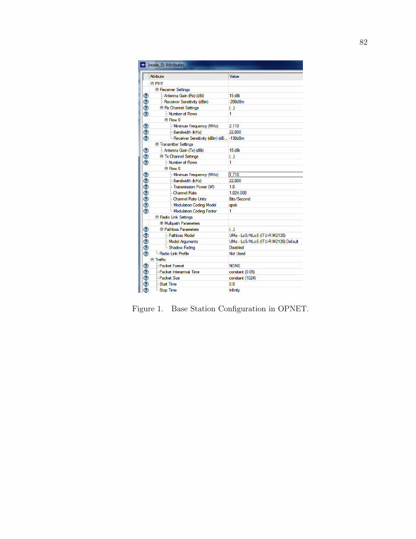
82

Figure 1. Base Station Configuration in OPNET.

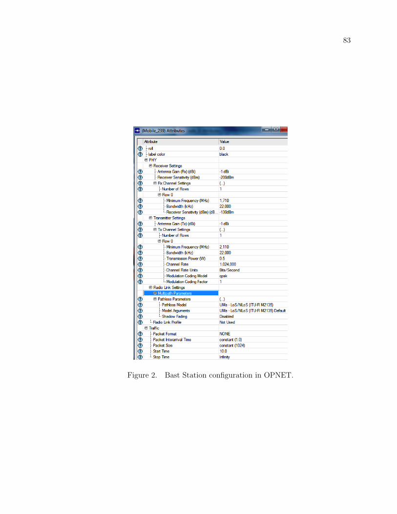
83

Figure 2. Bast Station configuration in OPNET.

VITA

Aribido Oluwaseun Joseph was born in June, 1987 at Kabba, Kogi State,

Nigeria. His love for academics began from childhood when he graduated best in his

primary school at NCAT staff school, zaria. He then attended Demonstration high

school where he exuded a rare sense of competitiveness to obtain the best West African

Examinations Council (WAEC) result in 2005. He went further to win the prestigious

Awokoya Memorial National competition in Chemistry, in september 2005 at the

annual Chemical Society of Nigeria (CSN) conference. On discovering his passion

for applied mathemtical sciences, he proceeded to study Electrical Engineering at

Ahmadu Bello University, Zaria and graduated with 2nd Class Upper division, and a

grand standing of 2nd position out of a class of over 120 students. During his masters

at Tennessee Tech, he researched on cutting edge wireless communications projects

that featured software algorithm design for Cognitive Radio on OPNET modeler

and Network Data Analysis using Random Matrix tools. His perpicacity was also

demonstrated in writing proposals for two research licenses which got approval for

OPNET modeler and Qualnet research software. At his leisure he loves hanging out

with his fiancee and friends at Life Church.

84

BIBLIOGRAPHY

85

86

[1] N. I. Sarkar and S. A. Halim, “A review of simulation of telecommunicationnetworks: simulators, classification, comparison, methodologies, and recommen-dations,” 2011.

[2] M. A. Waller and S. E. Fawcett, “Data science, predictive analytics, and bigdata: a revolution that will transform supply chain design and management,”Journal of Business Logistics, vol. 34, no. 2, pp. 77–84, 2013.

[3] M. A. Waller, S. E. Fawcett, and R. V. Hoek, “Thought leaders and thoughtfulleaders: advancing logistics and supply chain management,” Journal of BusinessLogistics, vol. 33, no. 2, pp. 75–77, 2012.

[4] K. Noyes, “These big data companies are ones to watch,” June 2014.

[5] R. F. Jeff Kelly, David Floyer, “Wikibon big data analytics survey, 2014,” August2014.

[6] J. Manyika, M. Chui, B. Brown, J. Bughin, R. Dobbs, C. Roxburgh, and A. H.Byers, “Big data: The next frontier for innovation, competition, and productiv-ity,” Journal of Business Logistics, 2011.

[7] M. Minelli, M. Chambers, and A. Dhiraj, “Big data technology,” Big Data,Big Analytics: Emerging Business Intelligence and Analytic Trends for Today’sBusinesses, pp. 61–88, 2012.

[8] A. Berson and S. J. Smith, Data warehousing, data mining, and OLAP. McGraw-Hill, Inc., 1997.

[9] P. Zikopoulos, C. Eaton, et al., Understanding big data: Analytics for enterpriseclass hadoop and streaming data. McGraw-Hill Osborne Media, 2011.

[10] F. Rusek, D. Persson, B. K. Lau, E. G. Larsson, T. L. Marzetta, O. Edfors, andF. Tufvesson, “Scaling up mimo: Opportunities and challenges with very largearrays,” Signal Processing Magazine, IEEE, vol. 30, no. 1, pp. 40–60, 2013.

[11] G. Wunder, M. Kasparick, S. ten Brink, F. Schaich, T. Wild, I. Gaspar,E. Ohlmer, S. Krone, N. Michailow, A. Navarro, et al., “5gnow: Challengingthe lte design paradigms of orthogonality and synchronicity,” in Vehicular Tech-nology Conference (VTC Spring), 2013 IEEE 77th, pp. 1–5, IEEE, 2013.

87

[12] J. Wishart, “The generalised product moment distribution in samples from anormal multivariate population,” Biometrika, pp. 32–52, 1928.

[13] P. Forrester, N. Snaith, and J. Verbaarschot, “Developments in random matrixtheory,” Random matrix theory, 2003.

[14] E. P. Wigner, “Random matrices in physics,” Siam Review, vol. 9, no. 1, pp. 1–23, 1967.

[15] V. A. Marcenko and L. A. Pastur, “Distribution of eigenvalues for some sets ofrandom matrices,” Sbornik: Mathematics, vol. 1, no. 4, pp. 457–483, 1967.

[16] Z. Bai and J. W. Silverstein, Spectral analysis of large dimensional random ma-trices. Springer, 2009.

[17] C. E. Ginestet, “Spectral analysis of large dimensional random matrices,” 2012.

[18] J. W. Silverstein and S.-I. Choi, “Analysis of the limiting spectral distribution oflarge dimensional random matrices,” Journal of Multivariate Analysis, vol. 54,no. 2, pp. 295–309, 1995.

[19] R. Couillet, M. Debbah, et al., Random matrix methods for wireless communi-cations. Cambridge University Press Cambridge, MA, 2011.

[20] Z. Bai and J. W. Silverstein, “No eigenvalues outside the support of the limitingspectral distribution of large-dimensional sample covariance matrices,” Annalsof probability, pp. 316–345, 1998.

[21] E. P. Wigner, “Characteristic vectors of bordered matrices with infinite dimen-sions i,” in The Collected Works of Eugene Paul Wigner, pp. 524–540, Springer,1993.

[22] V. Girko, “Circular law,” Theory of Probability & Its Applications, vol. 29, no. 4,pp. 694–706, 1985.

[23] A. Edelman and Y. Wang, “Random matrix theory and its innovative appli-cations,” in Advances in Applied Mathematics, Modeling, and ComputationalScience, pp. 91–116, Springer, 2013.

88

[24] R. C. Qiu, Smart Grid and Big Data: Theory and Practice. John Wiley andSons, 2013.

[25] D. Voiculescu, “Addition of certain non-commuting random variables,” Journalof functional analysis, vol. 66, no. 3, pp. 323–346, 1986.

[26] D. Voiculescu, Multiplication of certain non-commuting random variables. Inst.de Mat., 1985.

[27] U. Haagerup, “On voiculescus r-and s-transforms for free non-commuting randomvariables,” Free probability theory, vol. 12, pp. 127–148, 1997.

[28] R. Speicher, “Free probability and random matrices,” arXiv preprintarXiv:1404.3393, 2014.

[29] E. Altman, P. Dini, D. Miorandi, and D. Schreckling, “D2. 1.1 paradigms andfoundations of bionets research,” BIONETS (IST-2004-2.3. 4 FP6-027748) De-liverable (D2. 1.1), August, 2007.

[30] F. Hiai and D. Petz, The semicircle law, free random variables and entropy,vol. 77. American Mathematical Society Providence, 2000.

[31] U. Haagerup and F. Larsen, “Brown’s spectral distribution measure for¡ i¿r¡/i¿-diagonal elements in finite von neumann algebras,” Journal of FunctionalAnalysis, vol. 176, no. 2, pp. 331–367, 2000.

[32] J. Baik and J. W. Silverstein, “Eigenvalues of large sample covariance matricesof spiked population models,” Journal of Multivariate Analysis, vol. 97, no. 6,pp. 1382–1408, 2006.

[33] T. Tao, “Outliers in the spectrum of iid matrices with bounded rank pertur-bations,” Probability Theory and Related Fields, vol. 155, no. 1-2, pp. 231–263,2013.

[34] F. Benaych-Georges and J. Rochet, “Outliers in the single ring theorem,” arXivpreprint arXiv:1308.3064, 2013.

[35] D. S. Dean and S. N. Majumdar, “Large deviations of extreme eigenvalues ofrandom matrices,” Physical review letters, vol. 97, no. 16, p. 160201, 2006.

89

[36] Z. Ma et al., “Accuracy of the tracy–widom limits for the extreme eigenvaluesin white wishart matrices,” Bernoulli, vol. 18, no. 1, pp. 322–359, 2012.

[37] B. W. Silverman, Density estimation for statistics and data analysis, vol. 26.CRC press, 1986.

[38] M. Rosenblatt et al., “Remarks on some nonparametric estimates of a densityfunction,” The Annals of Mathematical Statistics, vol. 27, no. 3, pp. 832–837,1956.

[39] V. A. Epanechnikov, “Non-parametric estimation of a multivariate probabilitydensity,” Theory of Probability & Its Applications, vol. 14, no. 1, pp. 153–158,1969.

[40] Z. Lu and H. Yang, Unlocking the Power of OPNET Modeler. Cambridge Uni-versity Press, 2012.

[41] E. Weingartner, H. Vom Lehn, and K. Wehrle, “A performance comparison ofrecent network simulators,” in Communications, 2009. ICC’09. IEEE Interna-tional Conference on, pp. 1–5, IEEE, 2009.

[42] J. Pan and R. Jain, “A survey of network simulation tools: Current status andfuture developments,” Email: jp10@ cse. wustl. edu, 2008.

[43] adarshpal S. Sethi and V. Y. Hnatshin, The Practical OPNET User Guide forComputer Network. CRC PressTaylor & Francis Group, 2013.

[44] S. Parkvall, E. Dahlman, A. Furuskar, Y. Jading, M. Olsson, S. Wanstedt, andK. C. Zangi, “Lte-advanced-evolving lte towards imt-advanced.,” in VTC Fall,pp. 1–5, 2008.

[45] M. Series, “Guidelines for evaluation of radio interface technologies for imt-advanced,” tech. rep., ITU, Tech. Rep, 2009.

[46] K. Srinivasan, P. Dutta, A. Tavakoli, and P. Levis, “Understanding the causes ofpacket delivery success and failure in dense wireless sensor networks,” in Proceed-ings of the 4th international conference on Embedded networked sensor systems,pp. 419–420, ACM, 2006.

[47] I. H. InH, U. M. UMi, U. M. UMa, and R. M. RMa, “Guidelines for usingimt-advanced channel models,”

90

[48] A. M. Tulino and S. Verdu, “Random matrix theory and wireless communica-tions,” Communications and Information theory, vol. 1, no. 1, pp. 1–182, 2004.

[49] T. Guhr, A. Muller-Groeling, and H. A. Weidenmuller, “Random-matrix theo-ries in quantum physics: common concepts,” Physics Reports, vol. 299, no. 4,pp. 189–425, 1998.

[50] P. Buhlmann and S. Van De Geer, Statistics for high-dimensional data: methods,theory and applications. Springer, 2011.

[51] F. Luo, J. Zhong, Y. Yang, R. H. Scheuermann, and J. Zhou, “Application ofrandom matrix theory to biological networks,” Physics Letters A, vol. 357, no. 6,pp. 420–423, 2006.

[52] M. Potters, J.-P. Bouchaud, and L. Laloux, “Financial applications of randommatrix theory: Old laces and new pieces,” arXiv preprint physics/0507111, 2005.

[53] A. Utsugi, K. Ino, and M. Oshikawa, “Random matrix theory analysis of crosscorrelations in financial markets,” Physical Review E, vol. 70, no. 2, p. 026110,2004.

[54] V. Plerou, P. Gopikrishnan, B. Rosenow, L. A. N. Amaral, T. Guhr, and H. E.Stanley, “Random matrix approach to cross correlations in financial data,” Phys-ical Review E, vol. 65, no. 6, p. 066126, 2002.

[55] S. Sesia, I. Toufik, and M. Baker, LTE: the UMTS long term evolution. WileyOnline Library, 2009.

[56] D. Talbot, “One simple trick could disable a citys 4g phone network,” November14 2012.

[57] S. ORourke and A. Soshnikov, “Products of independent non-hermitian randommatrices,” Electron. J. Probab, vol. 16, no. 81, pp. 2219–2245, 2011.

[58] E. G. Larsson, O. Edfors, F. Tufvesson, and T. L. Marzetta, “Massive mimo fornext generation wireless systems,” arXiv preprint arXiv:1304.6690, 2013.

[59] C.-N. Chuah, D. N. C. Tse, J. M. Kahn, and R. A. Valenzuela, “Capacity scalingin mimo wireless systems under correlated fading,” Information Theory, IEEETransactions on, vol. 48, no. 3, pp. 637–650, 2002.

91

[60] S. A. Jafar and M. J. Fakhereddin, “Degrees of freedom for the mimo interferencechannel,” Information Theory, IEEE Transactions on, vol. 53, no. 7, pp. 2637–2642, 2007.

[61] R. R. Muller, M. Vehkapera, and L. Cottatellucci, “Blind pilot decontamination,”in Smart Antennas (WSA), 2013 17th International ITG Workshop on, pp. 1–6,VDE, 2013.

[62] C. A. Tracy and H. Widom, “The distributions of random matrix theory and theirapplications,” in New Trends in Mathematical Physics, pp. 753–765, Springer,2009.