An accurate finite element method for thenumerical solution of isothermal and

incompressible flow of viscous fluid, part I:computational analysis

B. Emek Abali ∗†

Abstract

Despite its numerical challenges, finite element method is used to compute viscous fluid flow. A consensuson the cause of numerical problems has been reached; however, general algorithms—allowing a robust andaccurate simulation for any process—are still missing. Either a very high computational cost is necessaryfor a direct numerical solution (DNS) or some limiting procedure is used by adding artificial dissipationto the system. These stabilization methods are often applied relative to the element size such that a localmonotonous convergence cannot be observed. We need a computational strategy for solving viscous fluidflow using only the balance equations. In this work, we present a general procedure solving fluid mechanicsproblems without use of any stabilization or splitting schemes. Hence its generalization to multiphysicsapplications is straight-forward. We discuss several numerical problems and present the methodology rigor-ously. Implementation is achieved by using open-source packages and the accuracy as well as the robustnessis demonstrated by comparing results to the closed-form solutions and by solving benchmarking problems.

1 IntroductionIsothermal flow of viscous fluid is governed by balance equations of mass and linear momentum:

∂ρ

∂t+ ∂viρ

∂xi= 0 , ∂ρvj

∂t+ ∂

∂xi

(viρvj − σij

)= ρgj , (1)

in Cartesian coordinates, where ρ denotes the mass density, vi the velocity, σij the non-convective flux term(Cauchy’s stress), gi the specific supply (gravitational forces); here and henceforth we apply Einstein’s sum-mation convention to repeated indices. In the case of Newtonian fluids such as water, oil, or alcohol, a linearrelation for stress furnishes the governing equations with accurate detail. This linear relation is the well-knownNavier–Stokes equation:

σij = (−p+ λdkk)δij + 2µdij , dij = 12

( ∂vi∂xj

+ ∂vj∂xi

), (2)

with the material constants λ, µ; and a new parameter p called hydrostatic pressure. Consider a control volumeinitially filled with homogeneous water, i.e., initial mass density is constant in space. Under conventionalpressure differences, we assume an incompressible flow, thus, the mass density remains constant in time. Forthe constant (in space and time) mass density, we obtain from the mass balance,

∂vi∂xi

= 0 , (3)

which is used for computing the pressure p. For an incompressible flow, the mechanical pressure − 13σii becomes

identical to the hydrostatic pressure p such that we handle p as the pressure generated in a pump. Velocity and

∗Corresponding author, email: bilenemek@abali.org†Technische Universitat Berlin, Institute of Mechanics

1

arX

iv:1

709.

0091

3v2

[cs

.CE

] 2

1 M

ar 2

018

pressure fields have to satisfy Eqs. (1)2 and (3).

In analytical mechanics, the aforementioned equations are fulfilled locally (in every infinitesimal point inspace). For a computation we discretize the space, for example with elements in finite size called the finite ele-ment method (FEM). Within each element, the analytical functions for the unknowns vi and p are representedby form (shape) functions with a local support, i.e., by means of a discrete element. The shape functions arenot smooth, they belong to Cn with a finite n. In other words, the unknowns are finitely differentiable anddepending on the governing equations and constitutive relations—from the mathematical analysis in [7]—weknow that the correct choice of the form functions for velocity and pressure is of paramount importance for a ro-bust computation. This so-called Ladyzhenskaya–Babuska–Brezzi (inf-sup compatibility) condition (LBBcondition) tells us how to adjust the shape functions of velocity and pressure in the case of an isothermal andincompressible flow. The prominent Taylor–Hood element is often used for the isothermal and incompressiblefluid flow problems. If one wants to include temperature deviation and electromagnetism into the computation,we fail to know the corresponding LBB condition for all shape functions (velocity, pressure, temperature, andelectromagnetic fields). For practical purposes, a robust computation without exploiting the LBB condition isuseful for a straight-forward extension to multiphysics applications.

Within a finite element, the governing equations are satisfied globally (over the domain of the element).There exists a general assumption that we can use the same local governing equations holding globally in finiteelements; however, this strategy leads to several numerical problems and to various proposals in [11, 29, 30, 48,45, 21, 10, 13, 25], for a review of such suggestions see [37]. These so-called stabilization methods introducea numerical parameter depending on the underlying mesh. This parameter induces an artificial viscosity inthe direction of the velocity change for suppressing and eliminating the numerical oscillations. Otherwise, acomputation is not possible since the numerical oscillations cause divergence of any numerical solution scheme.There are several successful implementations as in [32, 42, 31, 19, 28, 36, 20, 6]. From a practical point of view,such a stabilization method is very useful; however, introducing numerical parameters is problematic. Theseparameters are mesh dependent or they need to be tuned depending on the application. Tunable parameterscannot be measured such that an error estimation is not possible and most of the methods are conditionallystable, see [8]. A computation depending on the mesh size fails to show a local convergence, see references in[12] about accuracy problems of different techniques. We need to design a computation strategy for viscousfluid flows by using only physical (measurable) parameters such that a local monotonous convergence can beachieved by using FEM.

Indeed, numerical strategies exist for performing accurate simulations without numerical parameters. Byusing small elements—smaller than the characteristic length scale, for example Kolmogorov scale—we canovercome the numerical problems. This direct numerical simulation (DNS) is accurate and robust; however, it isoften not feasible without access to super-computers. There is another class of so-called splitting or projectionmethods such as Chorin’s method or its derivatives as in [17, 46, 47, 24, 9, 49, 14]. These methods are reliablebut it is challenging to adopt a splitting method in multiphysics.

The briefly mentioned problems are well known in the literature such that various new computation methodsare suggested for viscous flow problems. The (numerical) parameter free approach in [18] shows 2D and 3Dresults for stationary viscous flows without the nonlinear convection term (often called Stokes’s problem).Based on this idea an under-integrated mass matrix is used in [26, 34] to perform simulations without stabi-lization terms in 2D. Several mesh-dependent stabilization terms and their connections to mesh-independentstabilization methods are investigated in [15]. In [40] vorticity is used instead of velocity such that a new kindof splitting scheme is proposed for solving 3D problems. In [2] balance equations of mass, momentum, angularmomentum, and energy are used for performing 3D computations without numerical parameters; however, themethod already uses the energy equation making a generalization for the non-isothermal case quite difficult.In [41] vorticity is introduced as an independent term ensuring that the balance of moment of momentumis satisfied, only in 2D numerical solutions are performed without necessitating any (numerical) parameters.In [16] different strategies are performed for establishing 3D simulations. They are all based on writing thenonlinear convection term in a different (mathematically equivalent) form. In [22] a gradient-velocity-pressureformulation is suggested to solve 2D numerical experiments.

In this work, we discuss a special yet general case, namely an isothermal and incompressible flow. Forunderstanding the numerical problems, often, the pressure related numerical problems and velocity relatednumerical problems are studied separately. We use one balance equation for calculating the pressure and

2

another balance equation for calculating the velocity. These balance equations are coupled such that we failto uniquely identify which balance equation is to be used for pressure and velocity. Therefore, more robustnumerical strategies use both balance equations for both of the unknowns, this approach has already beenundertaken in Chorin’s method and then extensively used by the pressure stabilized Petrov–Galerkinmethod (PSPG). We use essentially the same strategy herein by motivating this approach from a differentperspective. Numerical problems are surpassed by incorporating the balance of angular momentum deliveringthe necessary smoothness for the pressure. Conventionally, the balance of angular momentum is neglected sinceit is already fulfilled locally by the balance of linear momentum (for the case of non-polar fluids). Furthermore,we discuss the integration by parts and suggest another approach than usually see in the literature. We explainin detail how to generate the weak form. Additionally, we emphasize that the weak form can be extended tofluid structure interaction or multiphysics problems very easily. We use open-source packages developed underthe FEniCS project1 and solve some academic examples in order to present the accuracy, local monotonousconvergence, and robustness of the proposed methodology. All codes are made public on the web site in [3] tobe used under the GNU Public license as in [23] for promoting an efficient scientific exchange as well as furtherstudies.

2 Variational formulationConsider the following general balance equation:(∫

Ωψ dv

)•

=∫

Ωz dv +

∫∂Ω

(f + φ) da , (4)

where the rate of the variable ψ is balanced with the supply term z acting volumetrically and with the fluxterms—convective f and non-convective φ—applying on the surface ∂Ω of a domain (control volume) Ω. Byusing Table 1 we can obtain the balance equations of mass, linear momentum, and angular momentum. The

Table 1: Volume densities, their supply and flux terms in the balance equations.

ψ z f φ

ρ 0 ni(wi − vi)ρ 0ρvj ρgj ni(wi − vi)ρvj σij

ρ(sj + εjklxkvl) ρ(`j + εjklxkgl) ni(wi − vi)ρ(sj + εjklxkvl) mij + εjklxkσil

domain may have its own velocity x•i = wi independent on the velocity of the fluid particle, vi. For a discussion

of the balance equations in a control volume with the domain velocity, we refer to [38, 39]. This domainvelocity can be chosen arbitrarily without affecting the underlying physics. For the sake of clarity, consider anexperiment where we record the motion of fluid by means of a high-speed camera. We may move the cameraarbitrarily, the motion of the fluid fails to alter. Normally we fix the camera to the laboratory frame such thatthe domain has no velocity, wi = 0. We will use this assumption of a fixed domain having two consequences.First, the time rate reads

(·)• = ∂(·)∂t

+ x•i

∂(·)∂xi

= ∂(·)∂t

+ wi∂(·)∂xi

= ∂(·)∂t

. (5)

Second, the rate of the infinitesimal volume element vanishes

dv• = ∂wi∂xi

dv = 0 . (6)

The domain velocity becomes important in computer methods for fluid structure interaction.

We start with the balance of mass for a fixed domain and apply the Gauss–Ostrogradskiy theorem∫Ω

∂ρ

∂tdv = −

∫∂Ωniviρda ,∫

Ω

∂ρ

∂tdv = −

∫Ω

∂viρ

∂xidv .

(7)

1The FEniCS computing platform, https://fenicsproject.org/

3

We assume that initially the fluid rests, vi(x, t = 0) = 0, and it is a homogeneous material, ρ(x, t = 0) = const.Moreover, we assume that the flow is incompressible, i.e., the mass density remains constant in time, ∂ρ/∂t = 0.Then the mass density is constant in space and time throughout the simulation leading to∫

Ωρ∂vi∂xi

dv = 0 . (8)

We multiply the latter with an arbitrary test function with the same rank of the integrand, i.e., a scalar. Havingan arbitrary test function ensures that the global condition holds locally as well. According to the Galerkinapproach, we will choose the test functions from the same space as the unknowns vi and p. Therefore, it isnatural to use δp and δvi as possible test functions. We emphasize that the choice of the scalar test function iscritical and we suggest to use ∫

Ωρ∂vi∂xi

δp dv = 0 , (9)

which is also the common procedure in the literature. Actually, by multiplying with the test function, we startedto utilize the discrete representation of the continuous velocity field. We omit a clear distinction in the notationsince we never use continuous and discrete functions together in one equation.

For the balance of linear momentum, the procedure is the same, we acquire for a fixed domain and incom-pressible flow ∫

Ω

(ρ∂vj∂t

)dv =

∫Ω

(ρgj − ρ

∂vivj∂xi

+ ∂σij∂xi

)dv . (10)

The integrand is a vector, hence, we use the test function δvi as being the usual case in the literature,∫Ω

(ρ∂vj∂t− ρgj + ρ

∂vivj∂xi

− ∂σij∂xi

)δvj dv = 0 . (11)

We refrain ourselves from inserting the mass balance, ∂vi/∂xi = 0, into the latter formulation. Since thiscondition is tested by δp, we cannot expect that it is fulfilled for the velocity distribution such that we chooseto enforce it by leaving the formulation as it is.

The same formalism is applied for the balance of angular momentum—for an incompressible flow ρ = const|x,twithin a fixed domain x•

i = wi = 0—leading to∫Ω

(ρ∂sj∂t

+ ρεjklxk∂vl∂t

)dv =

∫Ω

(ρ`j + ρεjkixkgi) dv +∫∂Ωni(− viρ(sj + εjklxkvl) +mij + εjklxkσil

)da ,∫

Ω

(ρ∂sj∂t

+ ρεjklxk∂vl∂t− ρ`j − ρεjkixkgi −

∂

∂xi

(− viρ(sj + εjklxkvl) +mij + εjklxkσil

))dv = 0 ,∫

Ω

(ρ∂sj∂t

+ ρεjklxk∂vl∂t− ρ`j − ρεjkixkgi + ρ

∂visj∂xi

+ ρεjklxk∂vivl∂xi

− ∂mij

∂xi− εjilσil − εjklxk

∂σil∂xi

)dv = 0 ,

(12)where ∂xi/∂xj = δij and the spin density si, its flux term (couple stress) mij , and its supply `i vanish for anon-polar medium like water (furnishing a symmetric stress). Then the angular momentum is identical to themoment of (linear) momentum,∫

Ωεjklxk

(ρ∂vl∂t− ρgl + ρ

∂vivl∂xi

− ∂σil∂xi

)dv = 0 ,∫

Ω

(ρ∂vl∂t− ρgl + ρ

∂vivl∂xi

− ∂σil∂xi

)dv = 0 ,

(13)

hence, in analytical mechanics, we can neglect it. However, we observe this term as an important term forresolving numerical challenges. Thus, we want to enforce it by multiplying the balance of angular momentumby a vector test function. If we multiply the balance of angular momentum for non-polar medium by δvl, thenthe outcome is identical to the variational form in Eq. (11). However, if we multiply by ∂δp/∂xl we obtain arestriction about the gradient of pressure, which is indeed the missing condition for the necessary numericalsmoothness for pressure. We may see this condition related to the LBB condition; however, we enforce it byusing an additional integral form instead of changing the order of shape functions. The same term multipliedby the mesh size is added in PSPG for the sake of a pressure stabilization. Herein we use it in equal manner for

4

every finite element independent of their size. The variational formulation for the balance of angular momentumreads ∫

Ω

(ρ∂vl∂t− ρgl + ρ

∂vivl∂xi

− ∂σil∂xi

)∂δp

∂xldv = 0 , (14)

which is one of the key contribution of this work providing stability and robustness.

We solve the transient integral forms in discrete time slices with a time step ∆t, this discretization in timecan be established by using Euler backwards method

∂vi∂t

= vi − v0i

∆t , (15)

where v0i indicates the value from the last time step. This implicit method is stable (for real valued problems)

and easy to implement.

3 Generating the weak formWe have to bring integral forms in Eqs. (9), (11), (14) into the same unit such that they can be summed up.We divide Eq. (9) by the mass density ρ and bring it to the unit of power. Equation (11) is already in the unitof power. We divide Eq. (14) by the mass density and multiply it by the time step ∆t and bring it also to theunit of power.

We rewrite the constitutive equation, σij = −pδij + τij , by combining all terms with dij into τij . Thesymmetric part of the velocity gradient, dij , thus, the term τij , include already velocity’s first derivative inspace. Therefore, we need to have a representation of the velocity function, which is at least C1 continuous.In the integral forms we observe another space derivative to τij leading to class C2 for velocity approximation.This condition can be weakened by integrating by parts. We emphasize that the integration by parts is appliedonly on the terms already including a differentiation in order to switch one differentiation to the test function.This strategy is not conventional. Often, integration by parts is used to all flux terms. We observe numericalproblems by using an integration by parts to all flux terms such that we suggest the method presented herein,which is another key contribution of this work. After bringing to the same unit and integrating by parts wherenecessary, we obtain

F1 =∫

Ωvi,iδp dv ,

F2 =∫

Ω

(ρvj − v0

j

∆t δvj − ρgjδvj + ρ(vivj),iδvj + p,iδvi + τijδvj,i

)dv−

∫∂Ωniτijδvj da ,

F3 =∫

Ω

((vj − v0

j )−∆tgj + ∆t(vivj),i −∆tρ

(−pδij + τij),i)δp,j dv ,

(16)

by using the usual comma notation for space derivative (),i = ∂()/∂xi. The weak form

Form∣∣Ω = F1 + F2 + F3 (17)

for one finite element reads zero by inserting the correct pressure and velocity distribution. A control volume isdecomposed into several elements such that the assembly over all elements, Form =

∑e F∣∣Ω, is the weak form

for the whole control volume. The sum over elements generate on the element boundaries the following term

JniτijK = Jni(σij + pδij)K (18)

with jump brackets J(·)K indicating the difference between the values of the quantity computed in adjacentelements. We use continuous form elements for pressure and velocity such that JnipK = 0, moreover, we enforceJniσijK = 0 relying on the balance of linear momentum on singular surfaces. Therefore, the integral term alongthe element boundaries vanish within the control volume. On the boundaries of the control volume eithervelocity or pressure is given. For the parts, where velocity is given, we choose δvi = 0 such that the boundaryterm vanishes. For the parts, where the water enters the domain with a prescribed pressure p against the planeoutward, ti = −pni, we obtain niτij = ni(σij + pδij) = tj + njp = 0. Therefore, all boundary terms vanish inthe weak form for an incompressible flow.

5

4 Algorithm and computationContinuous finite elements are used for all simulations in three-dimensional (3D) space. We use tetragonalelements with form functions of degree n = 1, hence, every element in 3D consists of four nodes. The primitivevariables are pressure and velocity and they are represented with their nodal values interpolated using the formfunctions. Concretely, 4 primitive variables P = p, v1, v2, v3 in three-dimensional space belong to

V =

P ∈ [Hn(Ω)]4 : P |∂Ω = given, (19)

where [Hn]4 is a 4-dimensional Hilbert space of class Cn as defined in [27] with additional differentiabilityproperties such that it is called a Sobolev space. The test functions, δP = δp, δv1, δv2, δv3, stem from thesame space

V =δP ∈ [Hn(Ω)]4 : δP |∂Ω = given

, (20)

which is the Galerkin approach. We use n = 1 for all simulations, in other words, we use the same linear formfunctions for pressure and for velocity. The spurious oscillations do not occur owing to the additional governingequation restricting the pressure gradient as well as the careful choice of terms to integrate by parts.

The weak form is nonlinear and coupled such that we need to linearize and solve it monolithically. For thelinearization we follow the ideas in [35, Part I, Sect. 2.2.3] and perform an abstract linearization using Newton’smethod at the partial differential level. The functional Form= F (P , δP ) is an integral of the function dependingon the primitive variables P and their variations (test functions) δP . We know the correct values of P at t0.The weak form is initially zero—we obtained it by subtracting left-hand sides from right-hand sides in thebalance equations. We search for the next time step, t = ∆t+ t0, by using the known P . This algorithm holdsfor every time steps, since we compute subsequently in time. We may describe the algorithm:

given: P (t) for x ,

find: P (t+ ∆t) at x ,

satisfying: F (P (t+ ∆t), δP ) = 0 .(21)

Now, by rewriting the unknowns P (t+ ∆t) in terms of the known values

P (t+ ∆t) = P (t) + ∆P (t) , (22)

we redefine the objective to searching for ∆P (t) instead of P (t+∆t). If ∆t is chosen sufficiently small, then thesolution is near to the known solution such that ∆P (t) is small. This condition leads to a Taylor expansionaround the known values, P (t), up to the (polynomial) order one

F (P + ∆P , δP ) = F (P , δP ) +∇PF (P , δP ) ·∆P , (23)

where we omit the time argument for the sake of clarity in notation. The expansion is linear in ∆P , hence weneed to construct a linear in ∆P differentiation operator, ∇P , which is established by the so-called Gateauxderivative:

∇PF (P , δP ) ·∆P = limε→0

ddεF (P + ε∆P , δP ) , (24)

where ε is an arbitrary parameter. Since we first differentiate in ε and then set the parameter ε equal to zero,only terms of order one in ∆P remain in the solution. By introducing the so-called Jacobian:

J(P , δP ) = ∇PF (P , δP ) , (25)

we rewrite the algorithm,given: P for x ,

find: ∆P at x ,

satisfying: F (P , δP ) + J(P , δP ) ·∆P = 0 .(26)

The last line is a linear function in ∆P such that we can solve the equation by obtaining ∆P and update thesolution in an iterative manner,

P := P + ∆P , (27)where “:=” is an assign operator in computational algebra. Here is the ultimate algorithm:

while |∆P | > TOL.solve ∆P , where F (P , δP ) + J(P , δP ) ·∆P = 0

P := P + ∆P

(28)

6

The term J ·∆P is computed automatically by means of symbolic differentiation implemented under the nameSyFi within the FEniCS project, see [4], [5]. This automatic linearization procedure allows us to use anynonlinear constitutive equation in the code. Herein we use a linear constitutive equation in order to achieve acomparison with closed-form solutions. The geometry is constructed in Salome2 by using NetGen algorithms3

for the triangulation. Then the mesh is transformed as explained in [1, Appendix A.3] and implemented in aPython code using packages developed by the FEniCS project, which is wrapped in C++ and solved in a Linuxmachine running Ubuntu.4

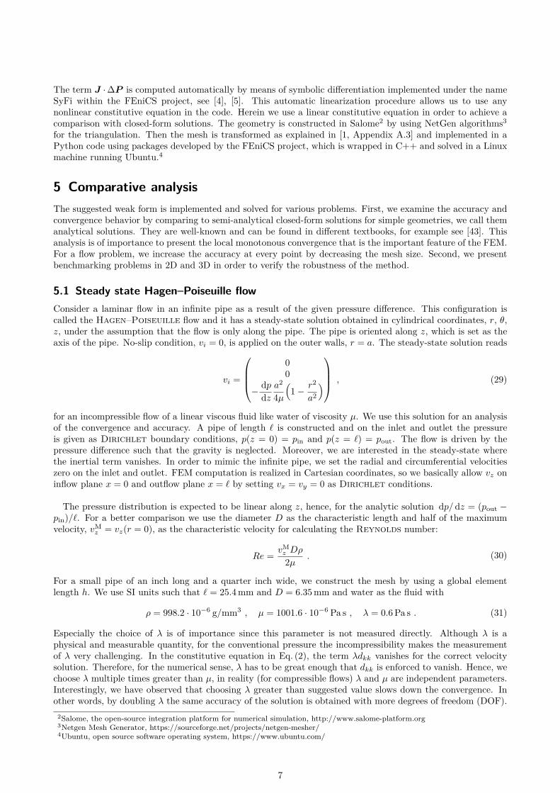
5 Comparative analysisThe suggested weak form is implemented and solved for various problems. First, we examine the accuracy andconvergence behavior by comparing to semi-analytical closed-form solutions for simple geometries, we call themanalytical solutions. They are well-known and can be found in different textbooks, for example see [43]. Thisanalysis is of importance to present the local monotonous convergence that is the important feature of the FEM.For a flow problem, we increase the accuracy at every point by decreasing the mesh size. Second, we presentbenchmarking problems in 2D and 3D in order to verify the robustness of the method.

5.1 Steady state Hagen–Poiseuille flowConsider a laminar flow in an infinite pipe as a result of the given pressure difference. This configuration iscalled the Hagen–Poiseuille flow and it has a steady-state solution obtained in cylindrical coordinates, r, θ,z, under the assumption that the flow is only along the pipe. The pipe is oriented along z, which is set as theaxis of the pipe. No-slip condition, vi = 0, is applied on the outer walls, r = a. The steady-state solution reads

vi =

00

− dpdz

a2

4µ

(1− r2

a2

) , (29)

for an incompressible flow of a linear viscous fluid like water of viscosity µ. We use this solution for an analysisof the convergence and accuracy. A pipe of length ` is constructed and on the inlet and outlet the pressureis given as Dirichlet boundary conditions, p(z = 0) = pin and p(z = `) = pout. The flow is driven by thepressure difference such that the gravity is neglected. Moreover, we are interested in the steady-state wherethe inertial term vanishes. In order to mimic the infinite pipe, we set the radial and circumferential velocitieszero on the inlet and outlet. FEM computation is realized in Cartesian coordinates, so we basically allow vz oninflow plane x = 0 and outflow plane x = ` by setting vx = vy = 0 as Dirichlet conditions.

The pressure distribution is expected to be linear along z, hence, for the analytic solution dp/dz = (pout −pin)/`. For a better comparison we use the diameter D as the characteristic length and half of the maximumvelocity, vM

z = vz(r = 0), as the characteristic velocity for calculating the Reynolds number:

Re = vMz Dρ

2µ . (30)

For a small pipe of an inch long and a quarter inch wide, we construct the mesh by using a global elementlength h. We use SI units such that ` = 25.4 mm and D = 6.35 mm and water as the fluid with

ρ = 998.2 · 10−6 g/mm3 , µ = 1001.6 · 10−6 Pa s , λ = 0.6 Pa s . (31)

Especially the choice of λ is of importance since this parameter is not measured directly. Although λ is aphysical and measurable quantity, for the conventional pressure the incompressibility makes the measurementof λ very challenging. In the constitutive equation in Eq. (2), the term λdkk vanishes for the correct velocitysolution. Therefore, for the numerical sense, λ has to be great enough that dkk is enforced to vanish. Hence, wechoose λ multiple times greater than µ, in reality (for compressible flows) λ and µ are independent parameters.Interestingly, we have observed that choosing λ greater than suggested value slows down the convergence. Inother words, by doubling λ the same accuracy of the solution is obtained with more degrees of freedom (DOF).

2Salome, the open-source integration platform for numerical simulation, http://www.salome-platform.org3Netgen Mesh Generator, https://sourceforge.net/projects/netgen-mesher/4Ubuntu, open source software operating system, https://www.ubuntu.com/

7

Its value does not change the convergence behavior, as long as it is great enough. In order to determine the valueof λ, we simply decreased until the maximum Re was achieved. Less than the used value leads to numericalproblems in the Newton–Raphson iterations.

By using a standard convergence analysis, we compare three different meshes starting with a global edgelength of tetrahedrons, h = 0.6 mm, then reducing it by half. Every time a new mesh is generated such thatthe number of nodes fail to increase exactly by 23 times in 3D. We use an unstructured mesh and the meshquality is nearly identical because of using the same algorithm on the relatively simple geometry. The expectedmonotonic convergence has been attained and can be seen in Fig. 1 for 2 different Reynold numbers. Two

(a) Re = 313 (b) Re = 940

Figure 1: Computation of steady state solution and its comparison to the analytic solution in a pipe for twodifferent Reynolds numbers.

important facts need to be underlined. First, the parabolic distribution of the velocity along the diameter isachieved even with a coarse mesh. Second, the relative error is 1.1% at r = 0 for a low Reynolds number and4.1% at r = 0 for a high Reynolds number by using mumps direct solver.

5.2 Starting Hagen–Poiseuille flowIn order to test the accuracy in the transient simulation, we use the same configuration and solve it transientlyin time. Since we have obtained the expected convergence in space discretization for the steady-state solution,we expect to have a monotonic convergence in time discretization, too. Therefore, we solve the same examplewith different time steps from t = 0 to t = 10 s with the initially applied pressure difference. For this case thereis a closed-form solution under the same assumptions as before,

vi =

00

− dpdz

a2

4µ

(1− r2

a2 −N∑n=1

8J0(Λn ra )

Λ3nJ1(Λn) exp(−Λ2

nτ)) , (32)

with τ = tµ/(ρa2) and Bessel functions (of the first kind) J0 and J1 with Λn being the roots of J0. Wecompute the (semi-)analytical solution by using SciPy packages for Bessel functions as well as its roots andchoose N = 50. By choosing the best mesh obtained from the convergence analysis in the steady-state case,namely the mesh with h = 0.15 mm, we compute the solution transiently in time by using different timesteps. We present in Fig. 2 the maximum value vz(r = 0, t) over time for different time steps showing theexpected convergence with decreasing time steps as well as the distribution at different time instants for thesmallest time step. In addition to the convergence in time, the relative error remains unchanged over time.We conclude that the suggested formalism is capable of simulating a simple, laminar, three-dimensional flow ofa linear viscous fluid accurately under a monotonic loading. The velocity and pressure distributions show noartifacts or mesh dependency as presented in Fig. 3. We have used mumps direct solver for achieving the highestaccuracy in the numerical solution. We emphasize that the pressure difference is applied instantaneously, whichis numerically challenging. For transient loading scenarios, there are various assumptions used for obtaining aclosed-form solution such that we omit to examine further. Based on the presented examples, we conclude thatthe approach delivers an accurate solution.

8

(a) ∆t = 1, 0.5, 0.25 s (b) ∆t = 0.25 s

Figure 2: Computation of transient solution and its comparison to the analytic solution in a pipe for Re = 313.

Figure 3: Velocity solution (direction as scaled arrows and magnitude as colors) and pressure solution (as colors)of the transient pipe flow at t = 5 s, shown on the half of the pipe (upper part: velocity and lowerpart: pressure) for Re = 313.

9

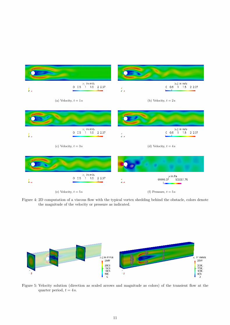
5.3 Flow over an obstacleAs suggested in [44] we implement a benchmarking problem in 2D and 3D. These benchmarking problems aredesigned to test a new method or code. They are well analyzed and the expected results are known. Bothproblems compute the viscous flow around an obstacle. The first problem is in 2D and we use the scaling as in[44] (for the 2D-2 case) such that the geometry is in meter length scale. A rectangle of ` = 2.2 m×H = 0.41 mhas a circular obstacle of radius 0.05 m located at (0.2, 0.2). On the upper and lower walls as well as on theobstacle fluid adheres to the resting walls. Fluid is pumped in from left and because of the unsymmetricalplacement of the obstacle, fluid around the hole gets perturbed. After a short amount of time, repeatingpattern of vortices appear behind the obstacle. This so-called von Karman vortex street is well-known in theliterature and a new numerical method has to be capable of reconstructing this phenomenon. On the right theDirichlet boundary condition for the pressure p = pref. is set. On the left the velocity profile:

vi =(vm

4y(H − y)H20

), (33)

is applied with vm = 1.5 m/s leading to the Reynolds number Re = 100 (inlet) for a linear viscous fluid ofρ = 1 kg/m3 and µ = 0.001 Pa s. Of course, such a fluid performing an incompressible flow is difficult to find inreality; however, the benchmark problem needs to be seen as a computationally challenging problem showingthe strength and robustness of the proposed code since a computation in such a low kinematic viscosity ν = µ/ρis known to generate numerical problems. By using ∆t = 0.001 s and bicgstab iterative solver with hypre-amgpreconditioner, we have computed up to 5 s as presented in Fig. 4.

For a comparison, the same problem is solved in [33, Section 3.4] by using the so-called incremental pressurecorrection scheme (IPCS) providing the same solution as herein. This splitting method is powerful for isother-mal case, but difficult to apply for non-isothermal cases.

The vortex shedding behind the obstacle occurs due to the boundary layer separation. This separation is dueto the changing pressure gradients as seen in Fig. 4(f). There are two stagnation points visible in front of andbehind the obstacle. Along the boundary of the obstacle, pressure gradient changes its sign at the top point.This change in pressure gradient resolves a so-called wake behind the obstacle, where the pressure is low suchthat the flow separates. We have modeled this phenomenon with the same element type and size around theboundary, in other words, without any special boundary layer modeling or whatsoever. Choosing Re = 100gives us an oscillating flow, between t = 2 s and t = 5 s one full cycle is surpassed. The pressure distributionalso shows the emerging vortices far away from the obstacle as moving wakes.

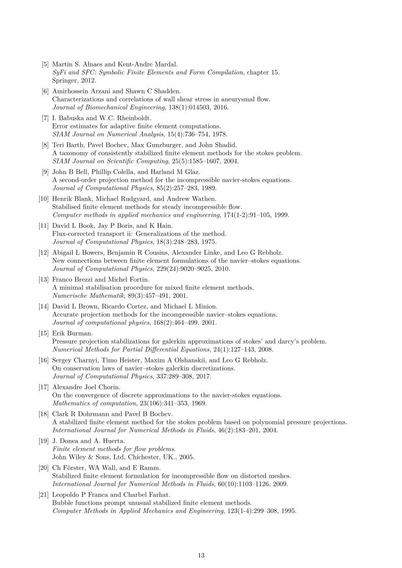
The second benchmark problem is in 3D. In analogy with the latter geometry, this time we simulate a pulsatingflow over a circular cylinder. The geometry is taken from the case 3D-3Z in [44] and rescaled to millimeterlength scale. The geometry is a box of 2500 mm x-length and H ×H cross section on yz-plane. A through holeof 100 mm diameter is placed asymmetrically, its center is at y = 200 mm and the y-length is H = 410 mm.This configuration leads to the same type of boundary layer separation. We apply a pulsating flow as follows

vi =

vm 16yz(H − y)(H − z)H4 sin

(πt

8

)00

, (34)

with the mean velocity of vm = 2250 mm/s. This parabolic function reads vm at the middle of the inflow planey = z = H/2 at t = 4 s. On the outflow plane x = 2500 mm we set the pressure as the reference pressure. Onthe walls and around the cylinder, no-slip condition, vi = 0, is implemented as Dirichlet boundaries. Wevisualize in Fig. 5 the velocity field and in Fig. 6 the pressure field at t = 4 s, when the maximum velocity onthe inflow plane has reached 2250 mm/s leading to a Reynolds number of Re = 100 with the diameter of thecylinder used as the characteristic length.

As expected, in the velocity solution we see the same distribution on the xy-plane as in 2D solution. Inyz-plane the distribution is manipulated because of the no-slip condition on the walls along z-axis. Behindthe cylinder the distribution is separated. In the middle there is a relatively slow back-flow. There is a smalldifference in the upper and lower distribution because of the non-symmetric placement of the obstacle. Thisfact can be seen in the pressure distribution as a difference between the highest and lowest position along the

10

(a) Velocity, t = 1 s (b) Velocity, t = 2 s

(c) Velocity, t = 3 s (d) Velocity, t = 4 s

(e) Velocity, t = 5 s (f) Pressure, t = 5 s

Figure 4: 2D computation of a viscous flow with the typical vortex shedding behind the obstacle, colors denotethe magnitude of the velocity or pressure as indicated.

Figure 5: Velocity solution (direction as scaled arrows and magnitude as colors) of the transient flow at thequarter period, t = 4 s.

11

Figure 6: Pressure solution as colors of the transient flow at the quarter period, t = 4 s.

cylinder. The pressure distribution along z-axis varies again effected by the no-slip condition on the walls alongz-axis. The total number of degrees of freedom (DOFs) for the 3D problem is 483 548 that is relatively smallfor such a computation in this detail. By using again bicgstab iterative solver with hypre-amg preconditioning,with the fixed time step, ∆t = 0.001 s, we could simulate on 13 CPUs via openmpi without facing any numericalproblems.

6 ConclusionA new method is proposed to compute fluid dynamics of isothermal and incompressible flows by means of FEM.We have rigorously investigated the convergence and the accuracy of the proposed approach by using closed-form solutions. Convergence in space and time is difficult to achieve in FEM for flow problems. The accuracyis only possible by using extremely high degrees of freedom. With the proposed method, we have attained agood accuracy with relatively coarse meshes. Local monotonic convergence in space and time is a remarkablequality of FEM and our method exploits this feature such that the proposed method is reliable. Moreover, wehave demonstrated the robustness of the implementation in open-source packages called FEniCS by solving flowaround the cylinder benchmark problems in 2D and 3D. Further research is being conducted as a second partincluding solution of real-life problems and verification of the proposed method with the aid of experimentalresults.

AcknowledgementB. E. Abali had the pleasure to have discussed and worked together with Prof. Omer Savas at the Universityof California, Berkeley.

References[1] B. E. Abali.

Computational Reality, Solving Nonlinear and Coupled Problems in Continuum Mechanics.Advanced Structured Materials. Springer, 2017.

[2] B. E. Abali, W. H. Muller, and D. V. Georgievskii.A discrete-mechanical approach for computation of three-dimensional flows.ZAMM-Journal of Applied Mathematics and Mechanics/Zeitschrift fur Angewandte Mathematik und

Mechanik, 93(12):868–881, 2013.[3] B. Emek Abali.

Technical University of Berlin, Institute of Mechanics, Chair of Continuum Mechanics and Material Theory,Computational Reality.

http://www.lkm.tu-berlin.de/ComputationalReality/, 2017.[4] Martin S. Alnaes and Kent-Andre Mardal.

On the efficiency of symbolic computations combined with code generation for finite element methods.ACM Transactions on Mathematical Software, 37(1), 2010.

12

[5] Martin S. Alnaes and Kent-Andre Mardal.SyFi and SFC: Symbolic Finite Elements and Form Compilation, chapter 15.Springer, 2012.

[6] Amirhossein Arzani and Shawn C Shadden.Characterizations and correlations of wall shear stress in aneurysmal flow.Journal of Biomechanical Engineering, 138(1):014503, 2016.

[7] I. Babuska and W.C. Rheinboldt.Error estimates for adaptive finite element computations.SIAM Journal on Numerical Analysis, 15(4):736–754, 1978.

[8] Teri Barth, Pavel Bochev, Max Gunzburger, and John Shadid.A taxonomy of consistently stabilized finite element methods for the stokes problem.SIAM Journal on Scientific Computing, 25(5):1585–1607, 2004.

[9] John B Bell, Phillip Colella, and Harland M Glaz.A second-order projection method for the incompressible navier-stokes equations.Journal of Computational Physics, 85(2):257–283, 1989.

[10] Henrik Blank, Michael Rudgyard, and Andrew Wathen.Stabilised finite element methods for steady incompressible flow.Computer methods in applied mechanics and engineering, 174(1-2):91–105, 1999.

[11] David L Book, Jay P Boris, and K Hain.Flux-corrected transport ii: Generalizations of the method.Journal of Computational Physics, 18(3):248–283, 1975.

[12] Abigail L Bowers, Benjamin R Cousins, Alexander Linke, and Leo G Rebholz.New connections between finite element formulations of the navier–stokes equations.Journal of Computational Physics, 229(24):9020–9025, 2010.

[13] Franco Brezzi and Michel Fortin.A minimal stabilisation procedure for mixed finite element methods.Numerische Mathematik, 89(3):457–491, 2001.

[14] David L Brown, Ricardo Cortez, and Michael L Minion.Accurate projection methods for the incompressible navier–stokes equations.Journal of computational physics, 168(2):464–499, 2001.

[15] Erik Burman.Pressure projection stabilizations for galerkin approximations of stokes’ and darcy’s problem.Numerical Methods for Partial Differential Equations, 24(1):127–143, 2008.

[16] Sergey Charnyi, Timo Heister, Maxim A Olshanskii, and Leo G Rebholz.On conservation laws of navier–stokes galerkin discretizations.Journal of Computational Physics, 337:289–308, 2017.

[17] Alexandre Joel Chorin.On the convergence of discrete approximations to the navier-stokes equations.Mathematics of computation, 23(106):341–353, 1969.

[18] Clark R Dohrmann and Pavel B Bochev.A stabilized finite element method for the stokes problem based on polynomial pressure projections.International Journal for Numerical Methods in Fluids, 46(2):183–201, 2004.

[19] J. Donea and A. Huerta.Finite element methods for flow problems.John Wiley & Sons, Ltd, Chichester, UK., 2005.

[20] Ch Forster, WA Wall, and E Ramm.Stabilized finite element formulation for incompressible flow on distorted meshes.International Journal for Numerical Methods in Fluids, 60(10):1103–1126, 2009.

[21] Leopoldo P Franca and Charbel Farhat.Bubble functions prompt unusual stabilized finite element methods.Computer Methods in Applied Mechanics and Engineering, 123(1-4):299–308, 1995.

13

[22] Guosheng Fu, Yanyi Jin, and Weifeng Qiu.Parameter-free superconvergent h(div)-conforming hdg methods for the brinkman equations.IMA Journal of Numerical Analysis, 2018.

[23] GNU Public.Gnu general public license.http://www.gnu.org/copyleft/gpl.html, June 2007.

[24] Katuhiko Goda.A multistep technique with implicit difference schemes for calculating two-or three-dimensional cavity flows.Journal of Computational Physics, 30(1):76–95, 1979.

[25] Volker Gravemeier.The variational multiscale method for laminar and turbulent flow.Archives of Computational Methods in Engineering, 13(2):249, 2006.

[26] Yinnian He and Jian Li.A stabilized finite element method based on local polynomial pressure projection for the stationary navier–

stokes equations.Applied Numerical Mathematics, 58(10):1503–1514, 2008.

[27] David Hilbert.The Foundations of Geometry.The Open Court Publishing Co., 1902.(transl. by Townsend, E.J.).

[28] Johan Hoffman and Claes Johnson.Computational turbulent incompressible flow, applied mathematics: body and soul 4.Springer, 2007.

[29] T. J. R. Hughes and A. Brooks.A theoretical framework for petrov-galerkin methods with discontinuous weighting functions: Application

to the streamline-upwind procedure.Finite elements in fluids, 4:47–65, 1982.

[30] T. J. R. Hughes, L. P. Franca, and M. Balestra.A new finite element formulation for computational fluid dynamics: circumventing the Babuska- Brezzi

condition: a stable Petrov- Galerkin formulation of the Stokes problem accommodating equal-orderInterpolation.

Computer Methods in Applied-Mechanics and Engineering, 59:85–99, 1986.[31] Thomas J. R. Hughes, Guglielmo Scovazzi, and Leopoldo P. Franca.

Encyclopedia of computational mechanics, volume 3, chapter 2 Multiscale and stabilized methods, pages5–59.

John Wiley & Sons, Ltd., 2004.[32] Dmitri Kuzmin and Stefan Turek.

Flux correction tools for finite elements.Journal of Computational Physics, 175(2):525–558, 2002.

[33] Hans Petter Langtangen and Anders Logg.Solving PDEs in Python: The FEniCS Tutorial I.Springer, 2016.

[34] Jian Li and Yinnian He.A stabilized finite element method based on two local gauss integrations for the stokes equations.Journal of Computational and Applied Mathematics, 214(1):58–65, 2008.

[35] Anders Logg, Kent-Andre Mardal, and Garth Wells.Automated solution of differential equations by the finite element method: The FEniCS book, volume 84.Springer Science & Business Media, 2012.

[36] Rainald Lohner.Applied computational fluid dynamics techniques: an introduction based on finite element methods.John Wiley & Sons, 2008.

[37] K. W. Morton.Finite element methods for non-self-adjoint problems.

14

In Peter Turner, editor, Topics in Numerical Analysis, volume 965, pages 113–148. Springer Berlin /Heidelberg, 1982.

[38] Wolfgang H. Muller and W. Muschik.Bilanzgleichungen offener mehrkomponentiger Systeme I. Massen- und Impulsbilanzen.Journal of Non-Equilibrium Thermodynamics, 8:29–46, 1983.

[39] W. Muschik and Wolfgang H. Muller.Bilanzgleichungen offener mehrkomponentiger Systeme II. Energie- und Entropiebilanz.Journal of Non-Equilibrium Thermodynamics, 8:47–66, 1983.

[40] Maxim A Olshanskii and Leo G Rebholz.Velocity–vorticity–helicity formulation and a solver for the navier–stokes equations.Journal of Computational Physics, 229(11):4291–4303, 2010.

[41] Artur Palha and Marc Gerritsma.A mass, energy, enstrophy and vorticity conserving (meevc) mimetic spectral element discretization for the

2d incompressible navier–stokes equations.Journal of Computational Physics, 328:200–220, 2017.

[42] R. Rannacher.Encyclopedia of computational mechanics, volume 3, chapter 6 Incompressible viscous flows, pages 155–181.John Wiley & Sons, Ltd., 2004.

[43] Omer Savas.Lecture notes, ME-260 A/B, Advanced Fluid Mechanics, Fall 2017.University of California, Berkeley, 2017.

[44] Michael Schafer, Stefan Turek, Franz Durst, Egon Krause, and Rolf Rannacher.Benchmark computations of laminar flow around a cylinder.In Flow simulation with high-performance computers II, pages 547–566. Springer, 1996.

[45] David J Silvester and N Kechkar.Stabilised bilinear-constant velocity-pressure finite elements for the conjugate gradient solution of the stokes

problem.Computer Methods in Applied Mechanics and Engineering, 79(1):71–86, 1990.

[46] Roger Temam.Sur l’approximation de la solution des equations de navier-stokes par la methode des pas fractionnaires (i).Archive for Rational Mechanics and Analysis, 32(2):135–153, 1969.

[47] Roger Temam.Sur l’approximation de la solution des equations de navier-stokes par la methode des pas fractionnaires (ii).Archive for Rational Mechanics and Analysis, 33(5):377–385, 1969.

[48] T. E. Tezduyar, S. Mittal, S.E. Ray, and R. Shih.Incompressible flow computations with stabilized bilinear and linear equal order interpolation velocity

pressure elements.Computer Methods in Applied Mechanics and Engineering, 95:221–242, 1992.

[49] Olgierd C Zienkiewicz and Ramon Codina.A general algorithm for compressible and incompressible flow—part i. the split, characteristic-based scheme.International Journal for Numerical Methods in Fluids, 20(8-9):869–885, 1995.

15