an adapted laplacian operator for hybrid quad… · an adapted laplacian operator for hybrid quad...
TRANSCRIPT
An Adapted Laplacian Operator ForHybrid Quad/Triangle Meshes
Alexander Pinzón Fernández
Universidad Nacional de Colombia
Facultad de Ingeniería, Departamento de Ingeniería de Sistemas e Industrial
Grupo de Investigación CIM@LAB
Bogotá, Colombia
2015
An Adapted Laplacian Operator ForHybrid Quad/Triangle Meshes
Alexander Pinzón Fernández
A thesis submitted in partial fulfillment of the requirements for the degree of:
Master in Systems Engineering and Computer Science
Advisor:Eduardo Romero Castro , Ph.D.
Research Area:Computer Graphics
Universidad Nacional de ColombiaFacultad de Ingeniería, Departamento de Ingeniería de Sistemas e Industrial
Grupo de Investigación CIM@LABBogotá, Colombia
2015
Dedicación
A Beatriz y Campo Elias mis padres que siempreme dieron la libertad de escoger, con su compren-sión y apoyo me permitieron dedicar mi tiempoa la ciencia.
A mis padres
Beatriz Fernández VargasCampo Elias Pinzón Rojas

Acknowledgment
I would like to thank my advisor professor Eduardo Romero and the CIM&LAB researchgroup for their support in this thesis.
I would like to thank all the workers in Colombia who fund public education with their work.
This work was supported in part by the Blender Foundation and the Google Summer ofCode program 2012 and 2013.

v
AbstractIn the last two decades three-dimensional modeling methods used by artists have been evolv-ing and developing rapidly thanks to the use of vector operators of differential geometry suchas the Laplacian operator. This operator allows modeling the behavior of complex appli-cations such as noise reduction, enhancement, remeshing, UV mapping, posing and skele-tonization, among others, in a simple way. The Laplacian operator is theoretically defined ina continuous and smooth domain, named manifold. In practice manifolds are often approx-imated by discrete polygon meshes composed by triangles and quadrangles which representthe real world three-dimensional objects with which the artists work. In these meshes, spec-tral structure is calculated using a discrete Laplacian operator, i.e. the discrete version ofthe Laplacian operator given by Pinkall in 1993. This approach only worked with trianglemeshes. In 2011 Xiong extended the operator to work exclusively with quad meshes. Thisthesis proposes an original extension of the Laplacian operator that allows working withhybrid meshes composed by triangles and quadrangles.
Along with the operator, this work presents new sculpting and modeling applications basedon enhancement. Additionally, applications on subdivision surfaces which use smoothing,mesh posing which use differential coordinates and skeletonization which use iterative con-tractions are developed. This series of applications demonstrates the quality, predictabilityand flexibility of the proposed operator.
The proposed operator was successfully used in new software tools in real production envi-ronment within 3D computer graphics software Blender. Currently these tools are availableas open source software.
ResumenEn las dos últimas décadas los métodos de modelado tridimensional utilizadas por los artistashan ido evolucionando y desarrollándose rápidamente, en parte gracias al uso de operadoresvectoriales de geometría diferencial, como el operador de Laplace. Este operador permitemodelar de una manera sencilla el comportamiento de aplicaciones complejas tales comola reducción de ruido, realce, remallado, mapeado UV, posado y esqueletonización, entreotros. Este operador Laplaciano es teóricamente definido en un dominio continuo y suavellamado variedad, las variedades son a menudo aproximadas por mallas discretas de polígonoscompuestas por triángulos y cuadrángulos que a su vez representan objetos tridimensionalesdel mundo real que los artistas trabajan. En estas mallas se calcula la estructura espectralcon el uso de algún operador Laplaciano discreto, la versión discreta del operador Laplacianopropuesta por Pinkall en el 1993 trabaja únicamente con mallas compuestas por triángulos,y la de Xiong en el 2011 trabaja exclusivamente con cuadrángulos. Esta tesis proponeuna extensión original del Operador Laplaciano que permite trabajar con mallas híbridascompuestas por triángulos y cuadrángulos.
vi
Junto con el operador, este trabajo presenta nuevas aplicaciones en esculpido y modelamientocon base en el realce, aplicaciones en subdivisión de superficies con el uso de suavizado,posado de mallas con el uso de coordenadas diferenciales y esqueletonización usando contrac-ción iterativa. Esta serie de aplicaciones demuestra la calidad, predictibilidad y flexibilidaddel operador propuesto.
El operador propuesto fue usado con exitoso en las nuevas herramientas del software paragráficos 3D por computadora Blender. Actualmente estas herramientas están disponiblescomo programas de código abierto.
Keywords: laplacian operator; smooth; enhance; sculpting; spectral mesh processing
Contents
Acknowledgement iv
Abstract v
1 Introduction 2
2 Mathematical Foundation and Background 42.1 Related work . . . . . . . . . . . . . . . . . . . . . . . . . . . . . . . . . . . 42.2 Manifolds . . . . . . . . . . . . . . . . . . . . . . . . . . . . . . . . . . . . . 62.3 Laplace Operator . . . . . . . . . . . . . . . . . . . . . . . . . . . . . . . . . 7
2.3.1 Discrete Laplace Operator Setting . . . . . . . . . . . . . . . . . . . . 7
3 Shape Inflation With an Adapted Laplacian Operator For Hybrid Quad/TriangleMeshes 83.1 Introduction . . . . . . . . . . . . . . . . . . . . . . . . . . . . . . . . . . . . 93.2 Related work . . . . . . . . . . . . . . . . . . . . . . . . . . . . . . . . . . . 103.3 Laplacian Smooth . . . . . . . . . . . . . . . . . . . . . . . . . . . . . . . . . 11
3.3.1 Gradient of Voronoi Area . . . . . . . . . . . . . . . . . . . . . . . . 113.3.2 Laplace Beltrami Operator . . . . . . . . . . . . . . . . . . . . . . . . 12
3.4 Proposed Method . . . . . . . . . . . . . . . . . . . . . . . . . . . . . . . . . 123.4.1 Laplace Beltrami Operator for Hybrid Quad/Triangle Meshes TQLBO 133.4.2 The Shape Inflation . . . . . . . . . . . . . . . . . . . . . . . . . . . . 15
3.5 Sculpting . . . . . . . . . . . . . . . . . . . . . . . . . . . . . . . . . . . . . 163.6 Subdivision surfaces . . . . . . . . . . . . . . . . . . . . . . . . . . . . . . . 173.7 Results . . . . . . . . . . . . . . . . . . . . . . . . . . . . . . . . . . . . . . . 183.8 Implementation . . . . . . . . . . . . . . . . . . . . . . . . . . . . . . . . . . 233.9 Conclusion and future work . . . . . . . . . . . . . . . . . . . . . . . . . . . 24
4 Mesh smoothing based on curvature flow operator in a diffusion equation 254.1 Synopsis . . . . . . . . . . . . . . . . . . . . . . . . . . . . . . . . . . . . . . 254.2 Benefits to Blender . . . . . . . . . . . . . . . . . . . . . . . . . . . . . . . . 254.3 Deliverables . . . . . . . . . . . . . . . . . . . . . . . . . . . . . . . . . . . . 264.4 Project Details . . . . . . . . . . . . . . . . . . . . . . . . . . . . . . . . . . 264.5 Project Schedule . . . . . . . . . . . . . . . . . . . . . . . . . . . . . . . . . 26
viii Contents
4.6 Mesh Smoothing . . . . . . . . . . . . . . . . . . . . . . . . . . . . . . . . . 274.7 Results and Conclusions . . . . . . . . . . . . . . . . . . . . . . . . . . . . . 28
5 Mesh Editing with Laplacian Deform 315.1 Synopsis . . . . . . . . . . . . . . . . . . . . . . . . . . . . . . . . . . . . . . 315.2 Benefits to Blender . . . . . . . . . . . . . . . . . . . . . . . . . . . . . . . . 315.3 Deliverables . . . . . . . . . . . . . . . . . . . . . . . . . . . . . . . . . . . . 325.4 Project Details . . . . . . . . . . . . . . . . . . . . . . . . . . . . . . . . . . 325.5 Project Schedule . . . . . . . . . . . . . . . . . . . . . . . . . . . . . . . . . 325.6 Laplacian Deform . . . . . . . . . . . . . . . . . . . . . . . . . . . . . . . . . 335.7 Testing Solvers . . . . . . . . . . . . . . . . . . . . . . . . . . . . . . . . . . 34
5.7.1 Hardware Specification . . . . . . . . . . . . . . . . . . . . . . . . . . 345.7.2 Software Specification . . . . . . . . . . . . . . . . . . . . . . . . . . 345.7.3 Numeric Solvers Used . . . . . . . . . . . . . . . . . . . . . . . . . . 35
5.8 Results . . . . . . . . . . . . . . . . . . . . . . . . . . . . . . . . . . . . . . . 36
6 Skeleton Extraction 396.1 Background . . . . . . . . . . . . . . . . . . . . . . . . . . . . . . . . . . . . 396.2 Contribution . . . . . . . . . . . . . . . . . . . . . . . . . . . . . . . . . . . . 426.3 Results and Conclusions . . . . . . . . . . . . . . . . . . . . . . . . . . . . . 44
7 Conclusion 46
Bibliography 46

List of Figures
3-1 A set of 48 successive shapes enhanced, from λ = 0.0 in blue to λ = −240.0
in red, with steps of −5.0. . . . . . . . . . . . . . . . . . . . . . . . . . . . . 83-2 Area of the Voronoi region around vi in dark blue.vj belong to the first neigh-
borhood around vi. αj and βj are opposite angles to edge −−−−→vj − vi. . . . . . . 113-3 t∗j1 ≡M vivjv
′j, t∗j2 ≡M viv
′jvj+1, t
∗j3 ≡M vivjvj+1 Triangulations of the quad
with common vertex vi proposed by [Xiong 2011] to define Mean LBO. . . . 133-4 The 5 basic triangle-quad cases with common vertex Vi and the relationship
with Vj and V ′j . (a) Two triangles [Desbrun 1999]. (b) (c) Two quads and onequad [Xiong 2011]. (d) (e) Triangles and quads (TQLBO) our contribution. . 14
3-5 Family of cups generated with our method, from a coarse model (a), (c): theshape, obtained from the Catmull-Clark Subdivision (b), (d), is inflated. Softconstraints, over the coarse model, is drawn in red and blue (c). . . . . . . . 17
3-6 (a) Original Model, (b) Model with Catmull-Clark Subdivision. Models withLaplacian smoothing: (c) and (d). Models with a first Laplacian filteringλ = 60.0, λe = 12.0 and before applying shape inflation: (e) and (f). . . . . 18
3-7 (a) Original Model. (b) Simple subdivision. (c), (d) (e) Laplacian smoothingwith λ = 7 and 2 iterations: (c) for triangles, (d) for quads, (e) for trianglesand quads chosen randomly. . . . . . . . . . . . . . . . . . . . . . . . . . . . 19
3-8 Top row: Original camel model in left. Shape inflation with λ = −30.0,λ = −100.0, λ = −400.0. Bottom row: Shape inflation with weight vertexgroup, λ = −50.0 and 2 iterations for the legs, λ = −200.0 and 1 iteration forthe head and neck. . . . . . . . . . . . . . . . . . . . . . . . . . . . . . . . . 20
3-9 The method is pose insensitive. The inflation for the different poses are similarin terms of shape. Top row: Original walk cycle camel model. Bottom row:Shape inflation with weight vertex group, λ = −400 and 2 iterations. . . . . 21
3-10Top row: (a) Original camel leg, (b) Inflate Brush used on leg within bluecircle, (c) Enhance Brush used on leg within red circle. Bottom row: (a)Original hand, (b) Inflate Brush used on fingers within blue circle, (c) EnhanceBrush used on fingers within red circle. . . . . . . . . . . . . . . . . . . . . . 21
3-11Performance of our dynamic Enhance Brush in terms of the sculpted verticesper second. Three models with 12K, 40K, 164K vertices used for sculpting inreal time. . . . . . . . . . . . . . . . . . . . . . . . . . . . . . . . . . . . . . 22
x List of Figures
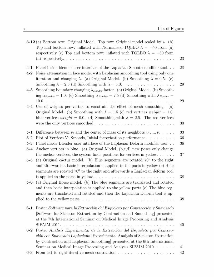
3-12 (a) Bottom row: Original Model. Top row: Original model scaled by 4. (b)Top and bottom row: inflated with Normalized-TQLBO λ = −50 from (a)respectively (c) Top and bottom row: inflated with TQLBO λ = −50 from(a) respectively. . . . . . . . . . . . . . . . . . . . . . . . . . . . . . . . . . . 23
4-1 Panel inside blender user interface of the Laplacian Smooth modifier tool. . . 284-2 Noise attenuation in face model with Laplacian smoothing tool using only one
iteration and changing λ. (a) Original Model. (b) Smoothing λ = 0.5. (c)Smoothing λ = 2.5 (d) Smoothing with λ = 5.0. . . . . . . . . . . . . . . . 29
4-3 Smoothing boundary changing λBorder factor. (a) Original Model. (b) Smooth-ing λBorder = 1.0. (c) Smoothing λBorder = 2.5 (d) Smoothing with λBorder =
10.0. . . . . . . . . . . . . . . . . . . . . . . . . . . . . . . . . . . . . . . . . 294-4 Use of weights per vertex to constrain the effect of mesh smoothing. (a)
Original Model. (b) Smoothing with λ = 1.5 (c) red vertices weight = 1.0,blue vertices weight = 0.0. (d) Smoothing with λ = 2.5. The red verticeswere the only vertices smoothed. . . . . . . . . . . . . . . . . . . . . . . . . . 30
5-1 Difference between vi and the center of mass of its neighbors v1, ..., v. . . . . 335-2 Plot of Vertices Vs Seconds, Initial factorization performance. . . . . . . . . 365-3 Panel inside Blender user interface of the Laplacian Deform modifier tool. . . 365-4 Anchor vertices in blue. (a) Original Model, (b,c,d) new poses only change
the anchor-vertices, the system finds positions for vertices in yellow. . . . . . 375-5 (a) Original cactus model. (b) Blue segments are rotated 70º to the right
and afterwards a basic interpolation is applied to the parts in yellow (c) Bluesegments are rotated 70º to the right and afterwards a Laplacian deform toolis applied to the parts in yellow. . . . . . . . . . . . . . . . . . . . . . . . . . 38
5-6 (a) Original Horse model. (b) The blue segments are translated and rotatedand then basic interpolation is applied to the yellow parts (c) The blue seg-ments are translated and rotated and then the Laplacian Deform tool is ap-plied to the yellow parts. . . . . . . . . . . . . . . . . . . . . . . . . . . . . . 38
6-1 Poster Software para la Extracción del Esqueleto por Contracción y Suavizado[Software for Skeleton Extraction by Contraction and Smoothing] presentedat the 7th International Seminar on Medical Image Processing and AnalysisSIPAIM 2011. . . . . . . . . . . . . . . . . . . . . . . . . . . . . . . . . . . . 40
6-2 Poster Análisis Experimental de la Extracción del Esqueleto por Contrac-ción con Suavizado Laplaciano [Experimental Analysis of Skeleton Extractionby Contraction and Laplacian Smoothing] presented at the 6th InternationalSeminar on Medical Image Processing and Analysis SIPAIM 2010. . . . . . . 41
6-3 From left to right iterative mesh contraction. . . . . . . . . . . . . . . . . . . 42

List of Figures xi
6-4 Left: The vertex xi moves along the line constraint. Right: the distance ofvertex xi to plane 1 and plane 2 when the position in every iteration changes. 43
6-5 sjSkeletonizer interface. (a) Open and display mesh. (b) Mesh contractedafter 4 iterations. (c) Skeleton obtained after surface simplification. . . . . . 44
6-7 Skeleton extracted from different models. (a) Dog model (b) Character model.(c) Person model. (d) Clay model. . . . . . . . . . . . . . . . . . . . . . . . . 45
6-6 Model with different poses and skeleton obtained with our skeleton extractionsoftware. . . . . . . . . . . . . . . . . . . . . . . . . . . . . . . . . . . . . . . 45

List of Tables
5-1 Vertices Vs Seconds, Laplacian Deform initial factorization performance. . . 35

1 Introduction
The discrete versions of the Laplace Beltrami Operator have been used in recent years forthe development of new geometric modeling tools. Pinkall [29] introduced the cotangentversion of the Laplace operator, which allowed finding the minimal surface when computinga discrete harmonic map with the Laplacian operator. This version has been widely studiedand applied in various problems of computer geometric modeling. This type of operator wasdefined over manifolds, i.e. continuous domains homeomorphic to Rn that are representedin pratice by polygon meshes. These polygons are generally composed of triangles andquadrangles. Working with the Laplacian operator in this hybrid composition is not amathematical challenge, most research only uses meshes composed by triangles [29, 14, 25, 37,3, 4, 20]. In recent studies [23, 43], the Laplacian operator may be used in meshes composedexclusively by quadrangles. However, from an artistic point of view, the topology and theway the edges, triangles and quadrangles are distributed, directly affects the processes ofanimation, interpolation, texturing, etc., as discussed by [26], who uses a manual connectionof a pair of vertices to perform animation processes and interpolation. It is then of paramountimportance to develop operators that easily interact with such meshes, eliminating the needof preprocessing the mesh to convert it to triangles and change the original topology.
Presently, modeling techniques that are able to generate a variety of realistic shapes areavailable [7] . Editing techniques have evolved from affine transformations to advancedtools such as sculpting [11, 17, 41], editing, creation from sketches [21, 19], and complexinterpolation techniques [37, 45]. Catmull-Clark based methods however require interactionwith a minimum number of control points for any operation to be efficient, or in otherwords, a unicity condition is introduced by demanding a smooth surface after any of theseshape operations. Hence, traditional modeling methods for subdividing surfaces from coarsegeometry have become widely popular [9, 40]. These works have generalized a uniform B-cubic spline knot insertion to meshes. Some of these add some type of control; for instancewith the use of creases to produce sharp edges [13] or the modification of some vertex weightsto locally control the zone of influence [5]. Nevertheless, these methods are difficult to useas they require a large number of parameters and a very tedious customization.
On the other hand, the proposed applications require a single parameter that controls theglobal curvature, which is used to maintain realistic shapes, creating a family of differentversions of the same object and therefore preserving the detail of the original model and arealistic appearance.

3
The shape inflation and shape exaggeration can thus be used as a type of brush in thesculpting process. When inflating a shape with other brushes the former ends up losingdetail when moving vertices [41]. In contrast, the presented enhance method inflates a meshby moving the vertices towards the reverse curvature direction, conserving the shape andsharp features of the model.
Contributions This work presents an extension of the Laplace Beltrami Operator for hy-brid quad/triangle meshes that have a larger mesh functionality spectrum than commontriangular or quadrangular meshes. The method eliminates the need of preprocessing andallows preservation of the original topology. Along with this operator, we propose a methodto generate a family of parameterized shapes, in a robust and predictable way. This methodenables customization of the smoothness and curvature obtained during the subdivision sur-faces process. Finally, a new brush for inflating the silhouette mesh features in modelingand sculpting is proposed.
The work is organized as follows: chapter 2 presents works related to the Laplacian operator,applications in digital sculpting, deformation, and offsetting methods for polygonal meshes.It also describes the theoretical framework of the Laplacian operator for polygon meshes;in chapter 3, we show the extension of the Laplacian Operator for hybrid meshes and theapplications of shape inflation ,subdivision of surfaces and sculpting; in chapter 4, we presentan application for mesh smoothing of the Laplacian operator extension here proposed, andimplemented into a well known software for computer modelling. Finally, in chapter 5, wepresent a successful application for mesh deformation and model re-posing based on differ-ential coordinates and the adaptation of this method to work with our Laplacian operatorextension.
2 Mathematical Foundation andBackground
This chapter studies basic mathematical foundations on differential geometry to understandthe differential operators and the Laplace Beltrami operator.
The differential geometry studies curvatures and geodesics [20]. These differential operatorsshow a deep relationship between the geometry (curvatures, geodesics) and topology of themanifold. They have been commonly used in computer geometric modeling applications overrecent years [35, 1].
2.1 Related work
Many tools, based on the Laplacian mesh processing, have been developed for modeling.These tools preserve the surface geometric details when using Laplacian operators for dif-ferent processes such as smoothing, enhancing, free-form deformation, fusion, morphing andother applications [34].
The most used discretization of Laplace Beltrami operator ∆Ω over a triangulated mesh Ω
was proposed by Pinkall [29].
∆Ω (u) = 12
∑j∈N1(i) (cotαj + cot βj) (xi − xj)
WhereN1is the 1-ring neighborhood, α and β are the opposite angles to edge between vertex iand vertex j. In this work the discrete Laplacian operator is used to find the minimal surfacebased on energy minimization strategy using the Dirichlet’s energy of the function u over amanifold represented by triangulated mesh Ω.
ED (u) = 12
´Ω
∣∣∇u∣∣2Taubin [42] was the first to treat the problem of noise reduction in digital polygonal meshesfrom a signal processing point of view. He extended Fourier analysis to signals definedon polygonal meshes, and observed that Fourier transformation is a decomposition of thesignal into eigenvectors of the Laplacian operator and reconstructs the signal with a linear
2.1 Related work 5
combination of these eigenvectors. Desbrun et al. [14] considered the same approach asTaubin, but they used a curvature normal (κn) based on a cotangent Laplacian operatorversion for noise reduction over a diffusion process. This is the most famous and popularLaplace Beltrami operator discretization [23]; many works for mesh smoothing and fairinghave been developed based on this Laplace Beltrami Operator (LBO) discretization [15, 25,36, 27]:
∂xi∂t
= −κini
−κini = 1A
∑j∈N1(i) (cotαj + cot βj)
where A is the area surrounding vertex i. This Laplacian operator L was used to reduce thenoise in a mesh X over a diffusion process.
The convergence of the Laplace Beltrami operator has been very important in fields suchas numerical analysis, given its implications in the simulation process and geometric partialdifferentials equations. Xu et al. [44] established the convergence of several discrete LaplaceBeltrami operators over triangulated meshes with numerical results that support the theoret-ical analysis. Over quadrilateral meshes, Liu et al. [23] presented a discrete Laplace BeltramiOperator based on a bilinear interpolation and its convergence over meshes composed onlyby quads.
In the work of Sorkine et al. [38] the Laplacian operator was used to re-pose a mesh whilepreserving geometry details of the surface. The details were stored in differential coordinatesδi for every vertex vi.
δi =∑
j∈N1(i)12
(cotαj + cot βj) (vi − vj)
The differential coordinates represent the difference between the absolute coordinate of viandthe center of mass of its immediate neighbors.
Offset methods for polygon meshing, based on the curvature defined by the Laplace Beltramioperator, have been developed. These methods adjust the shape offset by a constant distance,with high precision. Nevertheless, these methods fail to conserve sufficient detail because ofthe smoothing, a crucial issue which depends on the offset size [46]. In volumetric approaches,when using point-based representations, the offset boundary computation is based on thedistance field and therefore when calculating such offset, the topology of the model may bedifferent to the original [10].
Gal et al. [16] proposed automatic feature detection and shape edition with feature inter-relationship preservation. They defined salient surface features like ridges and valleys, char-acterized by their first and second order curvature derivatives (see [28]) and angle-based
6 2 Mathematical Foundation and Background
thresholds. Likewise, curves have also been classified as planar or non-planar, approximatedby lines, circles, ellipses and other complex shapes. In each case, the user defines an initialchange over several features which is propagated towards other features, based on the classi-fied shapes and the inter-relationships between them. This method works well with objectsthat have sharp edges, composed of basic geometric shapes such as lines, circles or ellipses.However, the method is very limited when models are smooth since it cannot find the properfeatures to edit.
Traditionally, digital sculpting has been approached under a polygonal representation or avoxel grid-based method. Brushes for inflation operations only depend on the vertex normal[41]. In grid-based sculpting, other operations allow the addition or removal of voxels, sinceproduction of polygonal meshes requires a processing of isosurfaces from volume [17]. Thedrawback comes from the difficulty of maintaining the surface details during larger scaledeformations.
In literature, several studies have described the skeleton extraction systems and differentmetrics that identify appropriate methods given a specific application [2]. One of the bestmethods reported in literature for the extraction of the skeleton is the Laplacian smoothingmethod given its advantages of homotopy representation and hierarchical connections be-tween parts. The skeleton extraction method permits the simplification of the dimension ofthe object while preserving the topological structure [12]. Au et. al. [3] present a skeletonextraction method based on iterative smoothing-contraction. In this method several con-straints are used to guarantee that the process converges to a skeleton formed by branchesand joints. The constraints are based on the Laplacian operator; the low frequencies of themesh are preserved with the use of an attractor to the original mesh, while the iterativesmoothing process removes high frequencies.
2.2 Manifolds
A manifold is a topological space M with the following properties:
If x ∈M , then there is some neighborhood N (x) and some integer n ≥ 0 such that N(x) ishomeomorphic to Rn [39].
Our work is related to manifolds that represent a surface in an three-dimensional EuclideanSpace. These manifolds are homeomorphic to R2.
The manifolds are represented by polygonal meshes with points connected by triangles andquads.
2.3 Laplace Operator 7
2.3 Laplace Operator
In computer graphics a manifold is often approximated by a discrete mesh [34], it is thereforenecessary to define a discrete Laplacian operator that acts on functions defined by suchmeshes.
Consider a smooth compact manifold M of dimension m isometrically embedded in a Eu-clidean space Rd.
Given a twice continuously differentiable function f ∈ C2 (M), let ∇Mf denote the gradientvector field of f on M .
The Laplace-Beltrami operator ∆M of f is defined as the divergence of the gradient; that is[39],
∂2f∂x2
+ ∂2f∂y2
+ ∂2f∂z2
= 0
∇2
Mf = ∆Mf = 0
∆Mf = div(∇Mf
)(2-1)
2.3.1 Discrete Laplace Operator Setting
Discrete Laplacian operators are linear operators that act on functions defined by meshes.These functions are defined by their values at the vertices.
Thus, if a mesh M has n vertices, then functions on M will be represented by vectors withn components and a mesh Laplacian will be described by an n× n matrix [34].
Locally, the Laplacian operator takes the difference between the value of a function at avertex and a weighted average of its values at the first-order or one-ring neighbor vertices,therefore a Laplacian matrix L has a local form that is given by
L (f)i = b−1i
∑j∈N(i)
wij (fi − fj)
where wijare the weights between the vertex i and the vertex j. b−1i are the factors depending
on the boundary region over vertex i. N (i) denotes the neighbors that share an edge withvertex i.
3 Shape Inflation With an AdaptedLaplacian Operator For HybridQuad/Triangle Meshes
Alexander Pinzón, Eduardo RomeroCimalab Research Group
Universidad Nacional de ColombiaBogota-Colombia
Email: [email protected], [email protected]
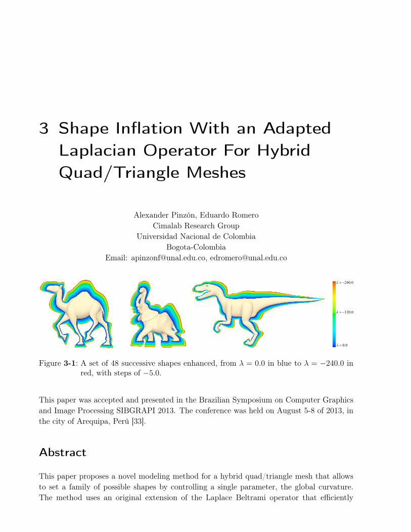
0.240
0.0
0.120
Figure 3-1: A set of 48 successive shapes enhanced, from λ = 0.0 in blue to λ = −240.0 inred, with steps of −5.0.
This paper was accepted and presented in the Brazilian Symposium on Computer Graphicsand Image Processing SIBGRAPI 2013. The conference was held on August 5-8 of 2013, inthe city of Arequipa, Perú [33].
Abstract
This paper proposes a novel modeling method for a hybrid quad/triangle mesh that allowsto set a family of possible shapes by controlling a single parameter, the global curvature.The method uses an original extension of the Laplace Beltrami operator that efficiently
3.1 Introduction 9
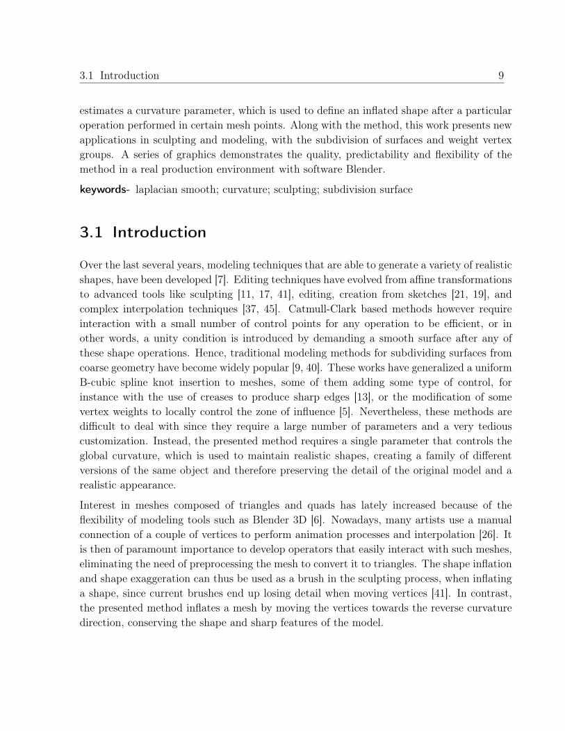
estimates a curvature parameter, which is used to define an inflated shape after a particularoperation performed in certain mesh points. Along with the method, this work presents newapplications in sculpting and modeling, with the subdivision of surfaces and weight vertexgroups. A series of graphics demonstrates the quality, predictability and flexibility of themethod in a real production environment with software Blender.
keywords- laplacian smooth; curvature; sculpting; subdivision surface
3.1 Introduction
Over the last several years, modeling techniques that are able to generate a variety of realisticshapes, have been developed [7]. Editing techniques have evolved from affine transformationsto advanced tools like sculpting [11, 17, 41], editing, creation from sketches [21, 19], andcomplex interpolation techniques [37, 45]. Catmull-Clark based methods however requireinteraction with a small number of control points for any operation to be efficient, or inother words, a unity condition is introduced by demanding a smooth surface after any ofthese shape operations. Hence, traditional modeling methods for subdividing surfaces fromcoarse geometry have become widely popular [9, 40]. These works have generalized a uniformB-cubic spline knot insertion to meshes, some of them adding some type of control, forinstance with the use of creases to produce sharp edges [13], or the modification of somevertex weights to locally control the zone of influence [5]. Nevertheless, these methods aredifficult to deal with since they require a large number of parameters and a very tediouscustomization. Instead, the presented method requires a single parameter that controls theglobal curvature, which is used to maintain realistic shapes, creating a family of differentversions of the same object and therefore preserving the detail of the original model and arealistic appearance.
Interest in meshes composed of triangles and quads has lately increased because of theflexibility of modeling tools such as Blender 3D [6]. Nowadays, many artists use a manualconnection of a couple of vertices to perform animation processes and interpolation [26]. Itis then of paramount importance to develop operators that easily interact with such meshes,eliminating the need of preprocessing the mesh to convert it to triangles. The shape inflationand shape exaggeration can thus be used as a brush in the sculpting process, when inflatinga shape, since current brushes end up losing detail when moving vertices [41]. In contrast,the presented method inflates a mesh by moving the vertices towards the reverse curvaturedirection, conserving the shape and sharp features of the model.
103 Shape Inflation With an Adapted Laplacian Operator For Hybrid Quad/Triangle
Meshes
Contributions
This work presents an extension of the Laplace Beltrami operator for hybrid quad/trianglemeshes, representing a larger mesh spectrum from what has been presented so far. Themethod eliminates the need of preprocessing and allows preservation of the original topology.Likewise, along with this operator, a method has been proposed to generate a family ofparametrized shapes, in a robust and predictable way. This method enables customizationof the smoothness and curvature obtained during the subdivision surfaces process. Finally,a new brush has been proposed for inflating the silhouette mesh features in modeling andsculpting.
This work is organized as follows: Section 3.2 presents works related to the Laplacian meshprocessing, digital sculpting, and offsetting methods for polygonal meshes; in section 3.3, thetheoretical framework of the Laplacian operator for polygon meshes is described; in section3.4, the method for shape inflation and applications of subdivision of surfaces and sculptingis presented; finally some Laplacian operator results using hybrid quad/triangle meshesare shown graphically, as well as results of the shape inflation applications in sculpting,subdivision and modeling.
3.2 Related work
Many tools have been developed for modeling, based on the Laplacian mesh processing.Thanks to the advantages of the Laplacian operator, these different tools preserve the surfacegeometric details when being used for different processes such as free-form deformation,fusion, morphing and other applications [37].
Offset methods for polygon meshing, based on the curvature defined by the Laplace Beltramioperator, have been developed. With enough precision, these methods adjust the shapeoffset by a constant distance. Nevertheless, these methods fail to conserve sufficient detailbecause of the smoothing, a crucial issue which depends on the offset size [46]. In volumetricapproaches, in the case of point-based representations, the offset boundary computation isbased on the distance field, and therefore when calculating such offset the topology of themodel may be different to the original [10].
[16] proposes automatic feature detection and shape edition with feature inter-relationshippreservation. They define salient surface features like ridges and valleys, characterized bytheir first and second order curvature derivatives, see [28], and angle-based threshold. Like-wise, curves have been also classified as planar or non-planar, approximated by lines, circles,ellipses and other complex shapes. In such cases, the user defines an initial change overseveral features which are propagated towards other features, based on the classified shapesand the inter-relationships between them. This method works well with objects that have
3.3 Laplacian Smooth 11
sharp edges, composed of basic geometric shapes such as lines, circles or ellipses. However,the method is very limited when models are smooth since it cannot find the proper featuresto edit.
Traditionally, digital sculpting has been approached under a polygonal representation or avoxel grid-based method. Brushes for inflation operations only depend on the vertex normal[41]. In grid-based sculpting, some other operations have allowed the addition or removal ofvoxels since production of polygonal meshes requires a processing of isosurfaces from volume[17]. The drawback comes from the difficulty of maintaining the surface details during largerscale deformations.
3.3 Laplacian Smooth
Computer objects, reconstructed from the real world, are usually noisy. Laplacian Smoothtechniques allow a proper noise reduction on the mesh surface with minimal shape changes,while still preserving a desirable geometry as well as the original shape.
Many smoothing Laplacian functionals regularize the surface energy by controlling the totalsurface curvature S.
E (S) =´Sκ2
1 + κ22dS
where κ1 and κ2 are the two principal curvatures of the surface S.
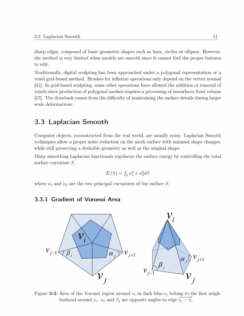
3.3.1 Gradient of Voronoi Area
iv
jv
1jv1jvj j
iv
jv1jv
1jvjj
Figure 3-2: Area of the Voronoi region around vi in dark blue.vj belong to the first neigh-borhood around vi. αj and βj are opposite angles to edge −−−−→vj − vi.

123 Shape Inflation With an Adapted Laplacian Operator For Hybrid Quad/Triangle
Meshes
Consider a surface S composed of a set of triangles around vertex vi. Let us define theVoronoi region of vi as shown in figure 3-2. The area change produced by the movement ofvi is called the gradient of Voronoi region [29, 14, 25].
∇A =1
2
∑j
(cotαj + cot βj) (3-1)
If the gradient in equation (3-1) is normalized by the total area of the 1-ring neighborhoodaround vi, the discrete mean curvature normal of a surface S is obtained, as shown inequation (3-2).
2κn =∇AA
(3-2)
3.3.2 Laplace Beltrami Operator
The Laplace Beltrami operator LBO noted as 4 is used for measuring the mean curvaturenormal to the Surface S [29].
4S = 2κn (3-3)
The LBO has desirable properties: the LBO points to the reverse direction of the minimalsurface area.
3.4 Proposed Method
This method exaggerates a shape using a Laplacian smoothing operator in the reverse di-rection, i.e., the new shape is a modified version in which those areas with larger curvatureare magnified. The operator amounts to a generator of a set of models, which conservesthe basic silhouette of the original shape. In addition, the presented approach can be eas-ily mixed with traditional or uniform subdivision of surfaces. This method is based on anoriginal extension of the Laplace Beltrami operator for hybrid quad/triangle meshes, mixingarbitrary types of meshes, exploiting the basic geometrical relationships and ensuring goodresults with few algorithm iterations.

3.4 Proposed Method 13
3.4.1 Laplace Beltrami Operator for Hybrid Quad/Triangle MeshesTQLBO
Given a mesh M = (V,Q, T ), with vertices V , quads Q, triangles T . The area of 1-ringneighborhood A (vi) corresponds to a sum of the quad faces A (Qvi) and the areas of thetriangular faces A (Tvi) adjacent to vertex vi.
A (vi) = A (Qvi) + A (Tvi)
*
1jt*
2jt
2j5j
3j4j
*
3jt
1j6j
iv iv
1jv 1jv
jv jv
jv jv jvjv
1jv
1j3j
4j
2j
5j
iv6j
*
4jt
Figure 3-3: t∗j1 ≡M vivjv′j, t∗j2 ≡M viv
′jvj+1, t
∗j3 ≡M vivjvj+1 Triangulations of the quad with
common vertex vi proposed by [Xiong 2011] to define Mean LBO.
Applying the mean average area, according to [43], from all possible triangulations, as showin figure 3-3, the area for quads A (Qvi) and triangles A (Tvi) is
A (vi) = 12m
m∑j=1
2m−1A (qj) +r∑
k=1
A (tk)
where q1, q2, ..., qj, ..., qm ∈ Qvi and t1, t2, ..., tk, ..., tr ∈ Tvi
A (vi) =1
2
m∑j=1
[A(t∗j1)
+ A(t∗j2)
+ A(t∗j3)]
+r∑
k=1
A (tk) (3-4)
Applying the gradient operator to (3-4)
∇A (vi) = 12
m∑j=1
[∇A
(t∗j1)
+∇A(t∗j2)
+∇A(t∗j3)]
+r∑
k=1
∇A (tk)
143 Shape Inflation With an Adapted Laplacian Operator For Hybrid Quad/Triangle
Meshes
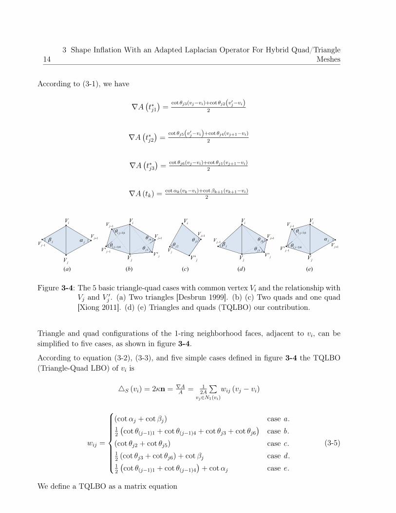
According to (3-1), we have
∇A(t∗j1)
=cot θj3(vj−vi)+cot θj2(v′j−vi)
2
∇A(t∗j2)
=cot θj5(v′j−vi)+cot θj4(vj+1−vi)
2
∇A(t∗j3)
=cot θj6(vj−vi)+cot θj1(vj+1−vi)
2
∇A (tk) = cotαk(vk−vi)+cotβk+1(vk+1−vi)2
1jViV
jV
1jV
jV '
1)1( j
1' jV4)1( j
6j
3j1jV
jj
iV
jV
1jV
iV
jV
1jV
jV '
5j
2j
iV
jV
1jV1jV 6j
3jj
1jViV
jV
1jV
1)1( j
1' jV4)1( j
j
)(a )(b )(c )(d )(e
jV '
Figure 3-4: The 5 basic triangle-quad cases with common vertex Vi and the relationship withVj and V ′j . (a) Two triangles [Desbrun 1999]. (b) (c) Two quads and one quad[Xiong 2011]. (d) (e) Triangles and quads (TQLBO) our contribution.
Triangle and quad configurations of the 1-ring neighborhood faces, adjacent to vi, can besimplified to five cases, as shown in figure 3-4.
According to equation (3-2), (3-3), and five simple cases defined in figure 3-4 the TQLBO(Triangle-Quad LBO) of vi is
4S (vi) = 2κn = ∇AA
= 12A
∑vj∈N1(vi)
wij (vj − vi)
wij =
(cotαj + cot βj) case a.12
(cot θ(j−1)1 + cot θ(j−1)4 + cot θj3 + cot θj6
)case b.
(cot θj2 + cot θj5) case c.12
(cot θj3 + cot θj6) + cot βj case d .12
(cot θ(j−1)1 + cot θ(j−1)4
)+ cotαj case e.
(3-5)
We define a TQLBO as a matrix equation
3.4 Proposed Method 15
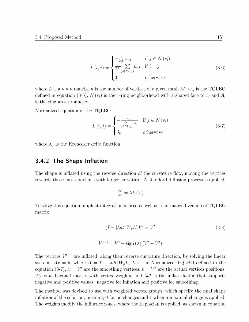
L (i, j) =
− 1
2Aiwij if j ∈ N (vi)
12Ai
∑j∈N(vi)
wij if i = j
0 otherwise
(3-6)
where L is a n×n matrix, n is the number of vertices of a given mesh M , wij is the TQLBOdefined in equation (3-5), N (vi) is the 1-ring neighborhood with a shared face to vi and Aiis the ring area around vi.
Normalized equation of the TQLBO
L (i, j) =
− wij∑
j∈N(vi)wij
if j ∈ N (vi)
δij otherwise(3-7)
where δij is the Kronecker delta function.
3.4.2 The Shape Inflation
The shape is inflated using the reverse direction of the curvature flow, moving the verticestowards those mesh portions with larger curvature. A standard diffusion process is applied:
∂V∂t
= λL (V )
To solve this equation, implicit integration is used as well as a normalized version of TQLBOmatrix
(I − |λdt|WpL)V ′ = V t (3-8)
V t+1 = V t + sign (λ) (V ′ − V t)
The vertices V t+1 are inflated, along their reverse curvature direction, by solving the linearsystem: Ax = b, where A = I − |λdt|WpL, L is the Normalized TQLBO defined in theequation (3-7), x = V ′ are the smoothing vertices, b = V t are the actual vertices positions,Wp is a diagonal matrix with vertex weights, and λdt is the inflate factor that supportsnegative and positive values: negative for inflation and positive for smoothing.
The method was devised to use with weighted vertex groups, which specify the final shapeinflation of the solution, meaning 0 for no changes and 1 when a maximal change is applied.The weights modify the influence zones, where the Laplacian is applied, as shown in equation
163 Shape Inflation With an Adapted Laplacian Operator For Hybrid Quad/Triangle
Meshes
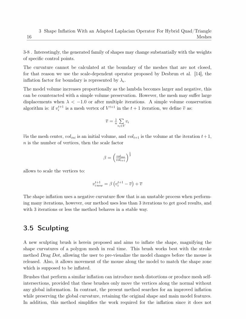
3-8 . Interestingly, the generated family of shapes may change substantially with the weightsof specific control points.
The curvature cannot be calculated at the boundary of the meshes that are not closed,for that reason we use the scale-dependent operator proposed by Desbrun et al. [14], theinflation factor for boundary is represented by λe.
The model volume increases proportionally as the lambda becomes larger and negative, thiscan be counteracted with a simple volume preservation. However, the mesh may suffer largedisplacements when λ < −1.0 or after multiple iterations. A simple volume conservationalgorithm is: if vt+1
i is a mesh vertex of V t+1 in the t+ 1 iteration, we define v as:
v = 1n
∑vi∈V
vi
vis the mesh center, volini is an initial volume, and volt+1 is the volume at the iteration t+1,n is the number of vertices, then the scale factor
β =(volini
volt+1
) 13
allows to scale the vertices to:
vt+1i new = β
(vt+1i − v
)+ v
The shape inflation uses a negative curvature flow that is an unstable process when perform-ing many iterations, however, our method uses less than 3 iterations to get good results, andwith 3 iterations or less the method behaves in a stable way.
3.5 Sculpting
A new sculpting brush is herein proposed and aims to inflate the shape, magnifying theshape curvatures of a polygon mesh in real time. This brush works best with the strokemethod Drag Dot, allowing the user to pre-visualize the model changes before the mouse isreleased. Also, it allows movement of the mouse along the model to match the shape zonewhich is supposed to be inflated.
Brushes that perform a similar inflation can introduce mesh distortions or produce mesh self-intersections, provided that these brushes only move the vertices along the normal withoutany global information. In contrast, the present method searches for an improved inflationwhile preserving the global curvature, retaining the original shape and main model features.In addition, this method simplifies the work required for the inflation since it does not

3.6 Subdivision surfaces 17
need different brushes for inflating, softening or styling. The inflated brush can do all theseoperations in a single step. Real-time brushes require the Laplacian matrix to be constructedwith the vertices that are within the sphere radius defined by the user, reducing the matrixto be processed. The center of this sphere depends on the place where the user clicks onthe canvas and also where the click is projected on the three-dimensional mesh. Specialhandling is required for the boundary vertices with neighbors that are not within the brushradius: these vertices mark the boundary though the curvature is not calculated there, butthey must be included in the matrix so that every vertex has their corresponding neighborswithin the selection. The sculpting Laplacian matrix reads as.
L (i, j) =
− wij∑
j∈N(vi)wij
if ‖vi − u‖ < r ∧ ‖vj − u‖ < r
0 if ‖vi − u‖ < r ∧ ‖vj − u‖ ≥ r
δij otherwise
where vj ∈ N (vi), u is the sphere center of radius r. The matrices should remove rows andcolumns of vertices that are not within the radius.
3.6 Subdivision surfaces
)(c)(a )(b
0.50,0.10 e0.0,0.10 e 0.8,0.80 e
0.0,0.10 e 0.2,0.80 e 0.60,0.50 e
0.0,0.10 e 0.50,0.10 e 0.8,0.80 e
0.60,0.50 e0.2,0.80 e0.0,0.10 e
)(d
Figure 3-5: Family of cups generated with our method, from a coarse model (a), (c): theshape, obtained from the Catmull-Clark Subdivision (b), (d), is inflated. Softconstraints, over the coarse model, is drawn in red and blue (c).
The Catmull-Clark subdivision transformation is used to smoothen a surface, as the limitof a sequence of subdivision steps [40]. This process is governed by a B-spline curve [24],performing a recursive subdivision transformation that refines the model into a linear in-terpolation that approximates a smooth surface. The model smoothness is automaticallyguaranteed [13].
183 Shape Inflation With an Adapted Laplacian Operator For Hybrid Quad/Triangle
Meshes
Catmull-Clark subdivision surface methods generate smooth and continuous models from acoarse model and produce quick results because of the simplicity of implementation. Nev-ertheless, changes to the global curvature are hardly implantable. The Catmull-Clark Sub-division Surfaces, together with shape inflation, can easily generate families of shapes bychanging a single parameter, allowing a model with very few vertices to be handled. Inpractice, this would allow an artist to choose a model from a similar set of options thatwould meet their needs without having to change each of the control vertices. Likewise, thepresented method allows the use of vertex weight paint over the control points. The weightscan be applied to a coarse model, followed by a Catmull-Clark subdivision where weightsare interpolated, producing weights with smooth changes in the influence zones, as shown infigure 3-5.c.
In equation 3-8, Wp is a diagonal matrix with weights corresponding to each vertex. Weightsat each vertex produce a different solution so that the matrix must be placed in the diffusionequation, since families that are generated may change substantially with the weight ofspecific control points.
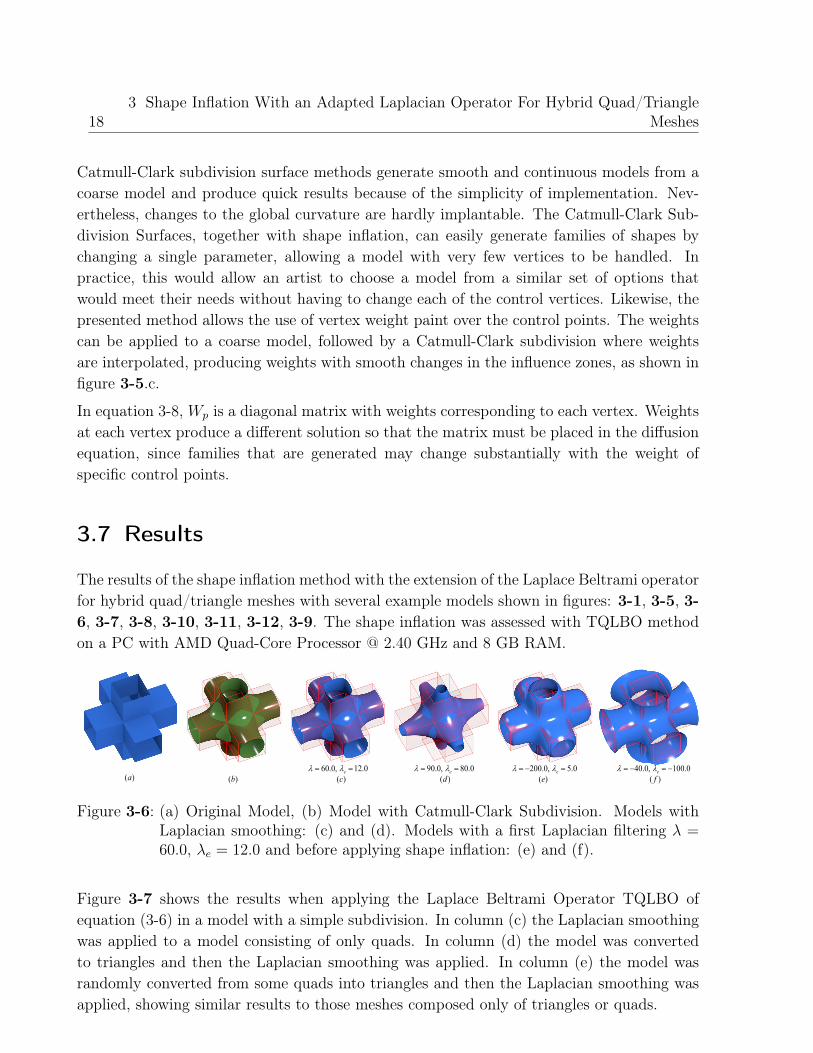
3.7 Results
The results of the shape inflation method with the extension of the Laplace Beltrami operatorfor hybrid quad/triangle meshes with several example models shown in figures: 3-1, 3-5, 3-6, 3-7, 3-8, 3-10, 3-11, 3-12, 3-9. The shape inflation was assessed with TQLBO methodon a PC with AMD Quad-Core Processor @ 2.40 GHz and 8 GB RAM.
0.12,0.60 e 0.80,0.90 e 0.5,0.200 e 0.100,0.40 e)(a )(b )(c )(d )(e )( f
Figure 3-6: (a) Original Model, (b) Model with Catmull-Clark Subdivision. Models withLaplacian smoothing: (c) and (d). Models with a first Laplacian filtering λ =60.0, λe = 12.0 and before applying shape inflation: (e) and (f).
Figure 3-7 shows the results when applying the Laplace Beltrami Operator TQLBO ofequation (3-6) in a model with a simple subdivision. In column (c) the Laplacian smoothingwas applied to a model consisting of only quads. In column (d) the model was convertedto triangles and then the Laplacian smoothing was applied. In column (e) the model wasrandomly converted from some quads into triangles and then the Laplacian smoothing wasapplied, showing similar results to those meshes composed only of triangles or quads.

3.7 Results 19
)(a )(b )(c )(d )(e
Figure 3-7: (a) Original Model. (b) Simple subdivision. (c), (d) (e) Laplacian smoothingwith λ = 7 and 2 iterations: (c) for triangles, (d) for quads, (e) for triangles andquads chosen randomly.
Methods using the Catmull-Clark Subdivision Surface and inflation allow the modificationof the curvature, as shown in figure 3-5. This test used a coarse cup model, in which thesubdivision was performed, followed by Laplacian smoothing and inflation. Figure 3-5.c, 3-5.d also shows the use of weight vertex groups over coarse models, with subdivision surfacesthat generate weights for the new interpolated vertices. These new weights were used forthe inflation obtained on the 6 cups that are at the right of the figure 3-5.d.

203 Shape Inflation With an Adapted Laplacian Operator For Hybrid Quad/Triangle
Meshes
0.4000.30
iterations2,0.50 iteration1,0.200
0.100Original
Figure 3-8: Top row: Original camel model in left. Shape inflation with λ = −30.0, λ =−100.0, λ = −400.0. Bottom row: Shape inflation with weight vertex group,λ = −50.0 and 2 iterations for the legs, λ = −200.0 and 1 iteration for the headand neck.
Laplacian smoothing applied with simple subdivision (see figure 3-6.c.) may produce similarresults to those obtained with Catmull-Clark (see figure 3-6.b.), whose models have averageequal triangles. The one obtained with the Laplacian smoothing is shown in panel (c),(d) and the curvature modified versions are in (e) and (f). As can be observed, differentversions of the original sketch can be obtained by parameterizing a single model value, a greatadvantage of the presented method. Figure 3-8 shows the generation of different versions ofa camel according to the λ parameter. In the top row the shape inflation results are shown.As λ becomes larger and negative, the resultant shape was inflated on the more convex parts,as shown in figure 3-1. The larger the λ parameter, the larger the model feature inflations.The bottom row of figure 3-8 shows the use of weighted vertex groups, specifying whichareas will be inflated. On the left, the inflation of the camel legs produces an organic aspect,notice that the border is not distorted and smooth.

3.7 Results 21
Figure 3-9: The method is pose insensitive. The inflation for the different poses are similarin terms of shape. Top row: Original walk cycle camel model. Bottom row:Shape inflation with weight vertex group, λ = −400 and 2 iterations.
The inflation of the silhouette’s features is predictable and invariant under isometric trans-formations, like those classically used in some animations (see Figure 3-9). In this figure, theanimation shows some camel poses during a walk. The inflation is performed at the neck andlegs, as shown in the bottom left camel in figure 3-9. Local modifications produced by thepose interpolation or animation rigging practically do not affect the result. There is a cleardifference despite the pose of the camel’s legs. The inflation method allows a flesh-like shapein the original pattern produced by the artist, this is due to the mesh restricted diffusionprocess so that small local changes are treated without affecting the global solution. Themethod therefore is rotation invariant since it depends exclusively on the normal mesh field.
(a) Original (b) Inflate Brush (c) Enhance Brush
Figure 3-10: Top row: (a) Original camel leg, (b) Inflate Brush used on leg within bluecircle, (c) Enhance Brush used on leg within red circle. Bottom row: (a)Original hand, (b) Inflate Brush used on fingers within blue circle, (c) EnhanceBrush used on fingers within red circle.

223 Shape Inflation With an Adapted Laplacian Operator For Hybrid Quad/Triangle
Meshes
0
0,2
0,4
0,6
0,8
1
1,2
1,4
0 500 1000 1500 2000 2500 3000 3500 4000 4500
Pro
cess
ing
tim
e in
sec
on
ds
Number of vertices
Sculpting Vertices per Second
12K
40K
164K
Figure 3-11: Performance of our dynamic Enhance Brush in terms of the sculpted verticesper second. Three models with 12K, 40K, 164K vertices used for sculpting inreal time.
Figure 3-10 shows the use of the Enhance Brush for sculpting in real time. One pass was usedwith the brush, shown by the blue and red radius. In figure 3-10.b the camel hoof shows theinflation intersection, which looks like two bubbles, a similar pattern that is observed on thefingers on the bottom row of the same figure. The silhouette inflation is observed in figure 3-10.c the main shape is retained together with either its finger or hoof details. Similar resultscan be obtained by using different brushes, however it would take several steps, while theEnhance Brush for shape inflation takes only a single step. For this reason, this new methodcan easily inflate organic features like muscles during the sculpting process. In figure 3-11the Enhance Brush performance is illustrated. In this experiment three models with 12K,40K and 164K vertices, were used. These models were sculpted with the Enhance Brush,each time the user selected a variable number of vertices for processing. The processing timefor 800 vertices in the camel hoof (40k model) only took 0.1 seconds, for 2600 vertices in theleg and neck (model 40k) it took 0.5 seconds. These times are suitable in real applicationssince an artist sculpts a model by parts and each part is represented by an average of about1800 vertices.

3.8 Implementation 23
)(a )(b )(c
Figure 3-12: (a) Bottom row: Original Model. Top row: Original model scaled by 4. (b)Top and bottom row: inflated with Normalized-TQLBO λ = −50 from (a)respectively (c) Top and bottom row: inflated with TQLBO λ = −50 from (a)respectively.
Tests with the Laplacian operator (equation 3-6) and its normalized version (equation 3-7),produce similar results if the triangles or quads that compose the mesh are about the samesize. The normalized version is more stable and predictable because it is not divided bythe area of the ring, which may be very small and cause numerical problems, as shown infigure 3-12.c bottom row. The shape inflation of the model with the normalized Laplacianoperator results in a more regular pattern. The model can be deformed with a normalizedversion of TQLBO with large λ (λ > 400) that can intersect itself but without any peaks.Figure 3-12.c shows different results due to the quads’ areas in the model. Quads with largerareas have smaller inflations (figure 3-12.c skull), and smaller quads have larger inflations(figure 3-12.c chin).
3.8 Implementation
The method was implemented as a modifier for modeling and brush for sculpting, on Blendersoftware [6] in C and C++ language programming. Working with Blender allowed themethod to be tested interactively against other methods, such as Catmull-Clark, WeightVertex Groups and Sculpting System.
To improve the performance, it was worked with the Blender mesh structure, visiting eachtriangle or quad and storing its corresponding index and the sum of the Laplacian weightsof the ring in a list so that only two visits were required for the list of mesh faces and two
243 Shape Inflation With an Adapted Laplacian Operator For Hybrid Quad/Triangle
Meshes
times for the edge list, if the mesh was not closed. This drastically reduced calculations,enabling real-time processing. In the construction of the Laplacian matrix, several indiceswere locked at vertices, which had face areas or edge lengths with zero value that could causespikes and bad results.
Under these conditions, the matrix of the equation 3-6 is sparse since the number of neighborsper vertex, corresponding to the number of data per row, is smaller compared to the totalnumber of vertices in the mesh. To solve the linear system equation 3-8 OpenNL [8] wasused, which is a a library for solving sparse linear systems.
3.9 Conclusion and future work
This work presented an extension of the Laplace Beltrami operator for hybrid quad/trianglemeshes that can be used in production environments and provides results similar to thoseobtained by working only with triangles or quads. This paper has introduced a new wayto change silhouettes in a mesh for modeling or sculpting in a few steps by means of thecurvature model modification while preserving its overall shape. In addition, a new modelingmethod has also been presented and some possible applications have been illustrated. Themethod works properly with isometric transformations, opening the possibility of introducingit to the process of animation.
We show that this tool may work in early modeling stages, when coarse models are used,allowing the shape generated by the Catmull-Clark subdivision surfaces to be modified andthereby avoiding edition of the vertices with a change of a single parameter.
Future work includes the analysis of theoretical relationships between the Catmull-Clarksubdivision surfaces and the Laplacian smoothing since they can produce very similar results.
Acknowledgment
We would like to thank anonymous friends for their support of our research.
This work was supported in part by the Blender Foundation, Google Summer of Codeprogram in 2012.
Livingstone elephant model is provided courtesy of INRIA and ISTI by the AIM@SHAPEShape Repository. The Hand model is courtesy of the FarField Technology Ltd. The Camelmodel by Valera Ivanov is licensed under a Creative Commons Attribution 3.0 UnportedLicense. Dinosaur and Monkey models are under public domain, courtesy of Blender Foun-dation.
4 Mesh smoothing based oncurvature flow operator in adiffusion equation
This work was accepted as part of the Blender [6] software, an open source 3D application formodeling, rendering, composing, video editing and game creation. The work was supportedby an awarded internship of the Google Summer of Code 2012 program, administered byGoogle Inc.
4.1 Synopsis
Objects reconstructed from the real world contain undesirable noise in many computer graph-ics applications. A Mesh smoothing may remove that noise while still preserving the geome-try and shape of the original model. This project aims to improve the mesh smoothing toolsuses by Blender software, using curvature flow operator in a diffusion equation, allowinghybrid meshes composed of triangles and quads to be worked with, and using the Laplacianoperator proposed by Pinzón and Romero [33].
4.2 Benefits to Blender
This project proposes a new and robust mesh smoothing tool that improves the appearanceof the surfaces of models. Usually, methods to scan computer graphics objects using theKinect ZCam need to remove the noise present at the time of capture. This mesh smoothingmethod produces higher quality results without shrinkage, while the smoothing tool currentlyused collapses after several iterations.
This mesh smoothing method allows hard and soft constraints on the positions of the meshpoints in order to maintain control over the shape, which facilitates the removal of noisegenerated during the sculpting, but without eliminating the desired details of the model.
26 4 Mesh smoothing based on curvature flow operator in a diffusion equation
4.3 Deliverables
• A new and robust mesh smoothing tool for Blender.
• Some documentation pages to be included in the manual.
• A technical document for developers to improve the method in the future.
• A tutorial explaining the use of the tool.
4.4 Project Details
The mesh smoothing algorithm was implemented as a diffusion equation for specific geometricstructures. The project was divided in four parts:
1. Initialization of data and necessary structures.
2. Computation of the Laplacian Matrix.
3. Definition of the sparse linear system.
4. Solution of the sparse linear system, using a preconditioned bi-conjugated gradientnumerical library.
Integration of the numerical library present in Blender to solve the sparse linear system
Generation of documentation and tutorials.
4.5 Project Schedule
• 3 weeks: Understanding the Blender source code and identifying the key points for theproject.
• 1 week: Definition of the data structures necessary to work with the Blender architec-ture.
• 1 week: Implementation of the methods for the initial configuration of the smoothingalgorithm. Implementation of the Laplacian matrix calculation.
• 2 weeks: Integration of the numerical library.
• 2 weeks: Formulation of the sparse linear system and implementation of the numericalmethod to solve it.
• 3 weeks: Formulation and implementation of the graphical user interface.
• 2 weeks: Testing the tool.
• 3 weeks: Generation of the documentation and tutorials.
4.6 Mesh Smoothing 27
4.6 Mesh Smoothing
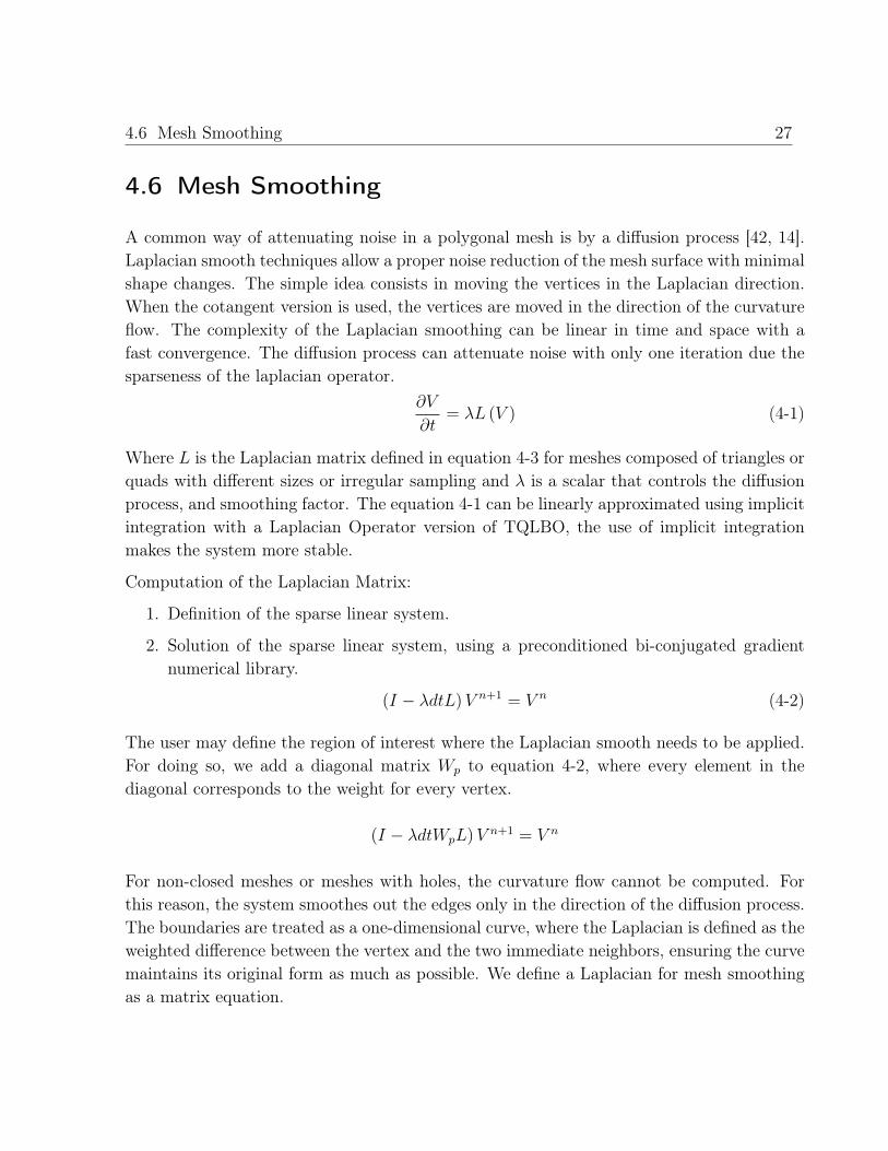
A common way of attenuating noise in a polygonal mesh is by a diffusion process [42, 14].Laplacian smooth techniques allow a proper noise reduction of the mesh surface with minimalshape changes. The simple idea consists in moving the vertices in the Laplacian direction.When the cotangent version is used, the vertices are moved in the direction of the curvatureflow. The complexity of the Laplacian smoothing can be linear in time and space with afast convergence. The diffusion process can attenuate noise with only one iteration due thesparseness of the laplacian operator.
∂V
∂t= λL (V ) (4-1)
Where L is the Laplacian matrix defined in equation 4-3 for meshes composed of triangles orquads with different sizes or irregular sampling and λ is a scalar that controls the diffusionprocess, and smoothing factor. The equation 4-1 can be linearly approximated using implicitintegration with a Laplacian Operator version of TQLBO, the use of implicit integrationmakes the system more stable.
Computation of the Laplacian Matrix:
1. Definition of the sparse linear system.
2. Solution of the sparse linear system, using a preconditioned bi-conjugated gradientnumerical library.
(I − λdtL)V n+1 = V n (4-2)
The user may define the region of interest where the Laplacian smooth needs to be applied.For doing so, we add a diagonal matrix Wp to equation 4-2, where every element in thediagonal corresponds to the weight for every vertex.
(I − λdtWpL)V n+1 = V n
For non-closed meshes or meshes with holes, the curvature flow cannot be computed. Forthis reason, the system smoothes out the edges only in the direction of the diffusion process.The boundaries are treated as a one-dimensional curve, where the Laplacian is defined as theweighted difference between the vertex and the two immediate neighbors, ensuring the curvemaintains its original form as much as possible. We define a Laplacian for mesh smoothingas a matrix equation.

28 4 Mesh smoothing based on curvature flow operator in a diffusion equation
L(i, j) =
− 12Aiwij if j ∈ N(vi) ∧ vi /∈ Boundary
12Ai
∑j∈N(vi)
wij if i = j ∧ vi /∈ Boundary
−eij if j ∈ N(vi) ∧ vi, vj ∈ Boundary2Ei
∑j∈N(vi)
eij if i = j ∧ vi, vj ∈ Boundary
0 otherwise
(4-3)
where L is a n×n matrix, n is the number of vertices of a given mesh M , wij is the TQLBOdefined in equation (3-5), N (vi) is the 1-ring neighborhood which has a shared face with vi,eij = 1
‖vi−vj‖ is the inverse length of the edge between vertices vi, vj, Ei =∑
j∈N(vi)
eij. Ai is
the ring area around vi.
4.7 Results and Conclusions
The developed user interface can be seen in figure 4-1. This tool allows the λ parameters forinner points and boundaries to be set, as well as to configure soft constraints using weightsdefined by vertices in “Vertex Group” and also to set strong constraints by independentlyapplying the algorithm in the axis X, Y or Z.
Figure 4-1: Panel inside blender user interface of the Laplacian Smooth modifier tool.
The tool developed can set the λdt parameter of equation 4-2. Using a small Lambda factor(λ < 1.0), noise can be removed without significantly affecting the geometry (see figure 4-
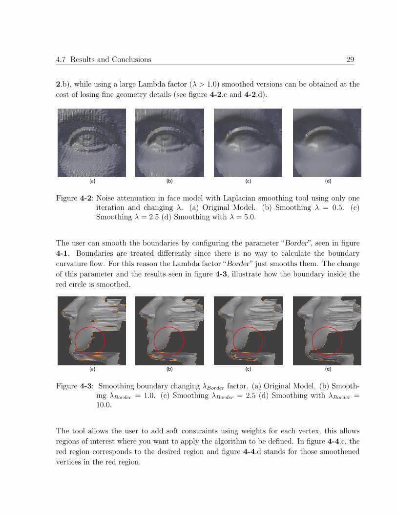
4.7 Results and Conclusions 29
2.b), while using a large Lambda factor (λ > 1.0) smoothed versions can be obtained at thecost of losing fine geometry details (see figure 4-2.c and 4-2.d).
(a) (b) (c) (d)
Figure 4-2: Noise attenuation in face model with Laplacian smoothing tool using only oneiteration and changing λ. (a) Original Model. (b) Smoothing λ = 0.5. (c)Smoothing λ = 2.5 (d) Smoothing with λ = 5.0.
The user can smooth the boundaries by configuring the parameter “Border”, seen in figure4-1. Boundaries are treated differently since there is no way to calculate the boundarycurvature flow. For this reason the Lambda factor “Border” just smooths them. The changeof this parameter and the results seen in figure 4-3, illustrate how the boundary inside thered circle is smoothed.
(a) (b) (c) (d)
Figure 4-3: Smoothing boundary changing λBorder factor. (a) Original Model. (b) Smooth-ing λBorder = 1.0. (c) Smoothing λBorder = 2.5 (d) Smoothing with λBorder =10.0.
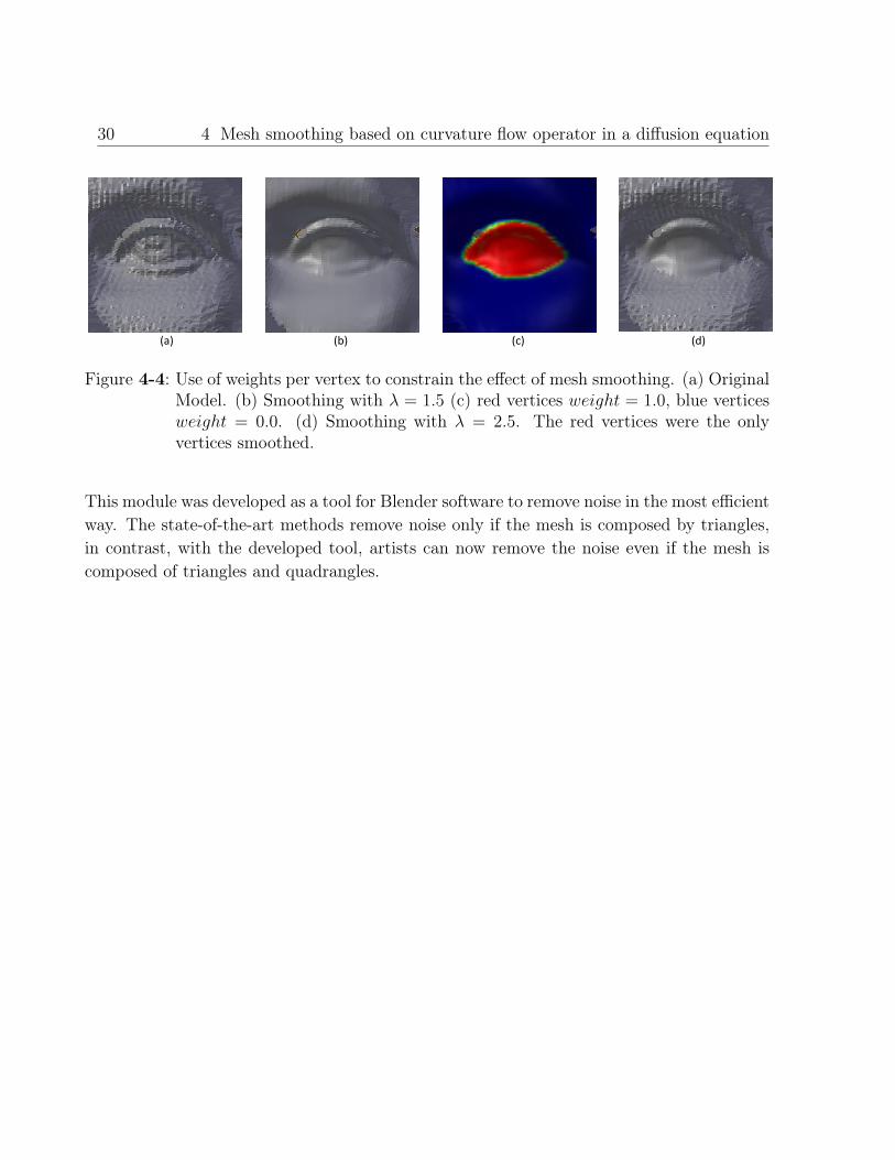
The tool allows the user to add soft constraints using weights for each vertex, this allowsregions of interest where you want to apply the algorithm to be defined. In figure 4-4.c, thered region corresponds to the desired region and figure 4-4.d stands for those smoothenedvertices in the red region.
30 4 Mesh smoothing based on curvature flow operator in a diffusion equation
(a) (b) (c) (d)
Figure 4-4: Use of weights per vertex to constrain the effect of mesh smoothing. (a) OriginalModel. (b) Smoothing with λ = 1.5 (c) red vertices weight = 1.0, blue verticesweight = 0.0. (d) Smoothing with λ = 2.5. The red vertices were the onlyvertices smoothed.
This module was developed as a tool for Blender software to remove noise in the most efficientway. The state-of-the-art methods remove noise only if the mesh is composed by triangles,in contrast, with the developed tool, artists can now remove the noise even if the mesh iscomposed of triangles and quadrangles.
5 Mesh Editing with LaplacianDeform
This work was accepted and completed for Blender [6] software, which is an open source 3Dapplication for modeling, animation, rendering, composing, video editing and game creation.In the Google Summer of Code 2013 program which was administered by Google Inc.
5.1 Synopsis
The mesh editing is generally done with affine transformations. Blender3D offers some toolsthat can transform vertices, such as “proportional editing object mode” with which thetransformation of some vertices is interpolated with the other vertices that are connectedwith the use of simple distance functions.
This project proposes to implement a method for mesh editing based on sketching linesdefined by the user and preserving the geometric details of the surface.
This method captures the geometric details using differential coordinates representations.The differential coordinates captures the local geometric information (curvature and direc-tion) of the vertex based on its neighbors. This method allows you to retrieve the bestpossible original model after changing the positions of some vertices by using the differentialcoordinates of the original model.
5.2 Benefits to Blender
This project proposes a new tool for Blender users that requires the preservation of geometricdetails of the surface during modeling, transformation and definition of the shape keys ofthe mesh vertices.
The method will allow novice users to edit any polygon mesh preserving the surface details.
This method allows the user to define new shape keys in a faster and more intuitive way.
32 5 Mesh Editing with Laplacian Deform
5.3 Deliverables
• A new mesh editing tool for Blender.
• Some pages of documentation to be included in the manual
• A technical document for developers to improve the method in the future.
• A tutorial explaining the use of the tool.
5.4 Project Details
The project is divided into eight parts:
1. Calculate the differential coordinates.
2. Store the fixed vertices (Hard constraints).
3. Store positions of the edited vertices.
4. Store the most representative vertex to retrieve rotation of every differential coordinate.
5. Solve the initial solution – in least-squares sense.
6. Rotate the differential coordinates based on initial solution and the most representativevertex.
7. Reconstruct the surface – in least-squares sense.
8. Generation of the documentation and tutorials.
5.5 Project Schedule
• 2 Weeks: Calculate the differential coordinates.
• 2 Weeks: Store the fixed vertices (Hard constraints).
• 2 Weeks: Store positions of the edited vertices.
• 2 Weeks: Compute initial solution.
• 2 Weeks: Rotate differential coordinates.
• 2 Weeks: Reconstruct the surface – in least-squares sense.
• 1 Week: Testing the tool and Define and implement graphical user integration.
• 2 Weeks: Generation of the documentation and tutorials.
5.6 Laplacian Deform 33
5.6 Laplacian Deform
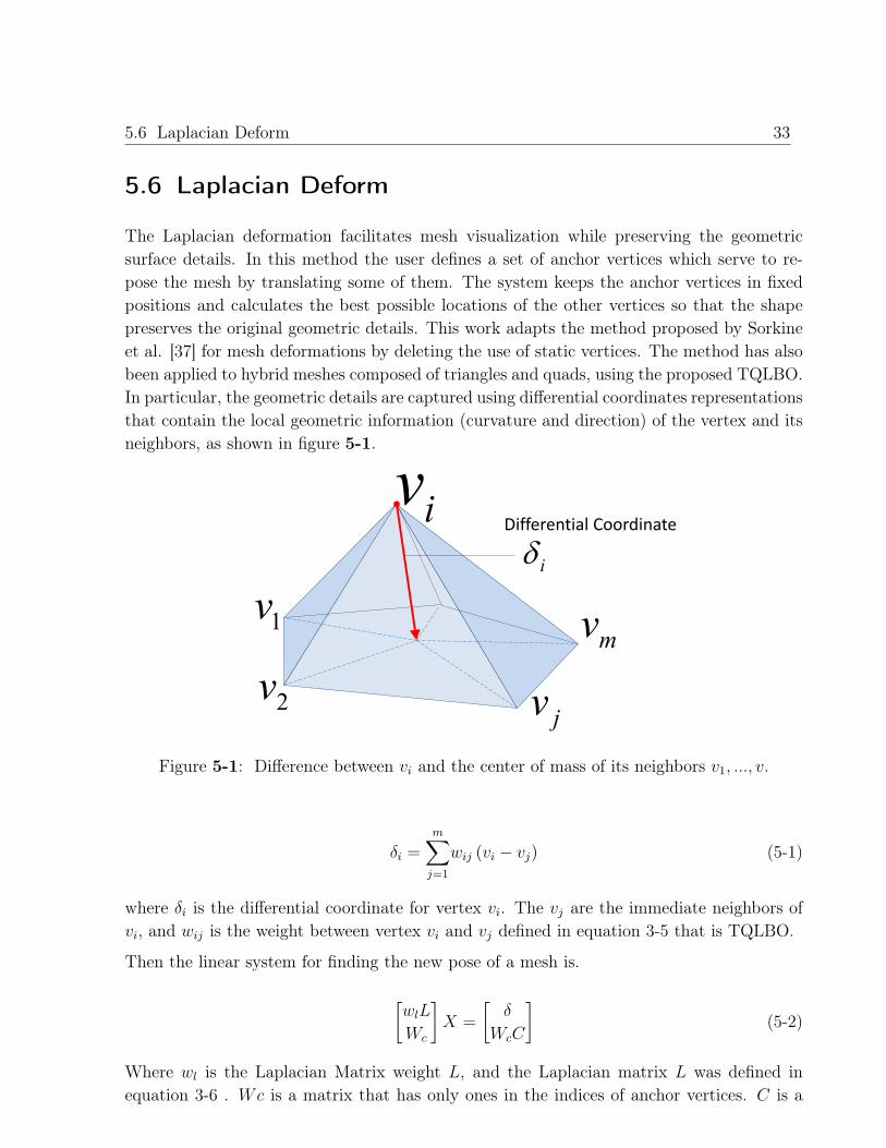
The Laplacian deformation facilitates mesh visualization while preserving the geometricsurface details. In this method the user defines a set of anchor vertices which serve to re-pose the mesh by translating some of them. The system keeps the anchor vertices in fixedpositions and calculates the best possible locations of the other vertices so that the shapepreserves the original geometric details. This work adapts the method proposed by Sorkineet al. [37] for mesh deformations by deleting the use of static vertices. The method has alsobeen applied to hybrid meshes composed of triangles and quads, using the proposed TQLBO.In particular, the geometric details are captured using differential coordinates representationsthat contain the local geometric information (curvature and direction) of the vertex and itsneighbors, as shown in figure 5-1.
i
1v
2v
mv
jv
iv Differential Coordinate
Figure 5-1: Difference between vi and the center of mass of its neighbors v1, ..., v.
δi =m∑j=1
wij (vi − vj) (5-1)
where δi is the differential coordinate for vertex vi. The vj are the immediate neighbors ofvi, and wij is the weight between vertex vi and vj defined in equation 3-5 that is TQLBO.
Then the linear system for finding the new pose of a mesh is.
[wlL
Wc
]X =
[δ
WcC
](5-2)
Where wl is the Laplacian Matrix weight L, and the Laplacian matrix L was defined inequation 3-6 . Wc is a matrix that has only ones in the indices of anchor vertices. C is a
34 5 Mesh Editing with Laplacian Deform
vector with coordinates of anchor vertices after several transformations. δ are the differentialcoordinates defined in equation 5-1.
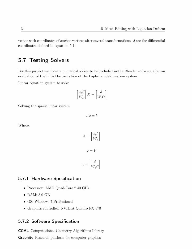
5.7 Testing Solvers
For this project we chose a numerical solver to be included in the Blender software after anevaluation of the initial factorization of the Laplacian deformation system.
Linear equation system to solve [wlL
Wc
]X =
[δ
WcC
]Solving the sparse linear system
Ax = b
Where:
A =
[wlL
Wc
]
x = V
b =
[δ
WcC
]
5.7.1 Hardware Specification
• Processor: AMD Quad-Core 2.40 GHz
• RAM: 8.0 GB
• OS: Windows 7 Professional
• Graphics controller: NVIDIA Quadro FX 570
5.7.2 Software Specification
CGAL Computational Geometry Algorithms Library
Graphite Research platform for computer graphics
5.7 Testing Solvers 35
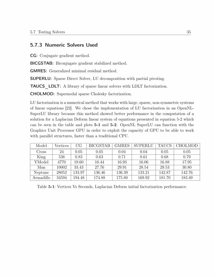
5.7.3 Numeric Solvers Used
CG: Conjugate gradient method.
BICGSTAB: Biconjugate gradient stabilized method.
GMRES: Generalized minimal residual method.
SUPERLU: Sparse Direct Solver, LU decomposition with partial pivoting.
TAUCS_LDLT: A library of sparse linear solvers with LDLT factorization.
CHOLMOD: Supernodal sparse Cholesky factorization.
LU factorization is a numerical method that works with large, sparse, non-symmetric systemsof linear equations [22]. We chose the implementation of LU factorization in an OpenNL-SuperLU library because this method showed better performance in the computation of asolution for a Laplacian Deform linear system of equations presented in equation 5-2 whichcan be seen in the table and plots 5-1 and 5-2. OpenNL SuperLU can function with theGraphics Unit Processor GPU in order to exploit the capacity of GPU to be able to workwith parallel structures, faster than a traditional CPU.
Model Vertices CG BICGSTAB GMRES SUPERLU TAUCS CHOLMODCross 24 0.05 0.05 0.04 0.04 0.05 0.05King 538 0.83 0.63 0.71 0.61 0.68 0.79
YModel 4770 19.60 16.44 16.93 16.06 16.88 17.95Man 10002 33.43 27.76 29.91 28.54 29.53 30.80
Neptune 28052 133.97 136.46 136.39 133.21 142.87 142.76Armadillo 34594 194.48 174.88 175.80 169.92 181.70 183.49
Table 5-1: Vertices Vs Seconds, Laplacian Deform initial factorization performance.
36 5 Mesh Editing with Laplacian Deform
0
20
40
60
80
100
120
140
160
180
200
0 5.000 10.000 15.000 20.000 25.000 30.000 35.000 40.000
Seco
nd
s
Vertices
Vertices Vs Seconds Initial Factorization Perfomance
CG
BICGSTAB
GMRES
SUPERLU
TAUCS
CHOLMOD
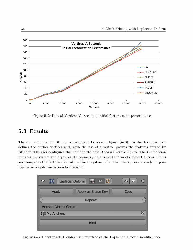
Figure 5-2: Plot of Vertices Vs Seconds, Initial factorization performance.
5.8 Results
The user interface for Blender software can be seen in figure (5-3). In this tool, the userdefines the anchor vertices and, with the use of a vertex, groups the features offered byBlender. The user configures this name in the field Anchors Vertex Group. The Bind optioninitiates the system and captures the geometry details in the form of differential coordinatesand computes the factorization of the linear system, after that the system is ready to posemeshes in a real-time interaction session.
Figure 5-3: Panel inside Blender user interface of the Laplacian Deform modifier tool.

5.8 Results 37
Figure (5-4) shows the Laplacian Deformation applied to a model with 173K vertices, onlyanchor vertices were used and are represented in blue. When the user applies several trans-formations (location, rotation, scale) to these anchor-vertices, the system finds a solutionand estimates the position of the vertices (in yellow). This method works in real time and
for doing so the matrix[wlL
Wc
]in equation (5-2) is LU decomposed only once, with LU fac-
torization, when the system initiates. Once the matrix is factorized, the system can solve theunknown variables in the order of milliseconds. Results are improved by solving the systemof equations several times, without LU factorization at every iteration, just the differentialcoordinates are adjusted since the differential coordinates can be rotated. Only four itera-tions were necessary for obtaining figure (5-4) but the system finds proper solutions withonly one iteration, when the angle of rotations are less thanπ.
(a) (b) (c) (d)
Figure 5-4: Anchor vertices in blue. (a) Original Model, (b,c,d) new poses only change theanchor-vertices, the system finds positions for vertices in yellow.
Figure 5-5 shows a comparison after making a single transformation that rotates the partsin blue 70º to the right. Results using a bicubic interpolation are shown in 5-5.b observehow the main trunk loses its shape when rotated. The propagation of changes made by theLaplacian deformation (figure 5-5.c) for the same transformation, shows better results.

38 5 Mesh Editing with Laplacian Deform
70º
70º
(a) (b) (c)
Figure 5-5: (a) Original cactus model. (b) Blue segments are rotated 70º to the right andafterwards a basic interpolation is applied to the parts in yellow (c) Blue seg-ments are rotated 70º to the right and afterwards a Laplacian deform tool isapplied to the parts in yellow.
The Laplacian Deformation tool allows the user to change the model’s pose while preservingthe geometry details. In figure 5-6.b and 5-6.c observe the horse’s new pose after fivetransformations and one head rotation. In figure 5-6.b the shape and details are lost at everychange using basic interpolation. In constrast, figure 5-6..c illustrates how the new pose ofthe horse looks more natural, above all for the body and neck. This comparison indicatesthat the Laplacian Deform method allows any transformation to be applied without any lossof detail.
(a) (b) (c)
g g g
Figure 5-6: (a) Original Horse model. (b) The blue segments are translated and rotated andthen basic interpolation is applied to the yellow parts (c) The blue segmentsare translated and rotated and then the Laplacian Deform tool is applied to theyellow parts.

6 Skeleton Extraction
Part of this work was accepted and presented as a poster titled Software para la Extraccióndel Esqueleto por Contracción y Suavizado [Software for Skeleton Extraction by Contractionand Smoothing] at 7th International Seminar on Medical Image Processing and AnalysisSIPAIM 2011. The conference was held on December 6-8 of 2011, in Bucaramanga, Colombia[31], the poster thumbnail is shown in figure 6-1.
Part of this work was accepted and presented as a poster titled Análisis Experimental de laExtracción del Esqueleto por Contracción con Suavizado Laplaciano [Experimental Analysisof Skeleton Extraction by Contraction and Laplacian Smoothing] at the 6th InternationalSeminar on Medical Image Processing and Analysis SIPAIM 2010. The conference was heldon December 1-4 of 2010, in the city of Bogotá, Colombia [30], the poster thumbnail is shownin figure 6-2.
6.1 Background
Skeleton extraction not only reduces the dimensionality but also represents a three-dimensionalobject as a uni-dimensional structure [12].
Skeleton extraction uses the natural shrink produced by Laplacian smoothing [25], to itera-tively contract the mesh until the volume inside the surface is about zero (see figure 6-3).This method stretches the mesh to guarantee that the object preserves, as much as possible,the original topology constraint [3].
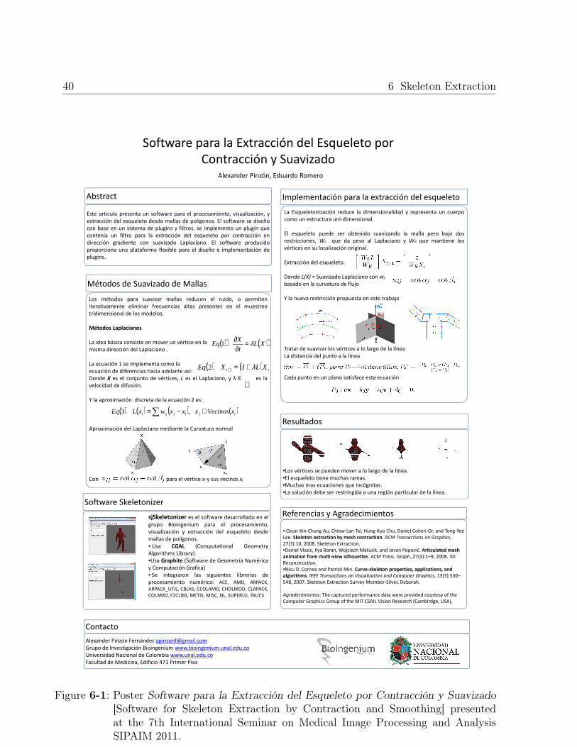
40 6 Skeleton Extraction
Software para la Extracción del Esqueleto porSoftware para la Extracción del Esqueleto por
Contracción y SuavizadoContracción y SuavizadoAlexander Pinzón, Eduardo Romero
AbstractAbstract
Este articulo presenta un software para el procesamiento, visualización, yEste articulo presenta un software para el procesamiento, visualización, y
extracción del esqueleto desde mallas de polígonos. El software se diseño
con base en un sistema de plugins y filtros, se implemento un plugin que
contenía un filtro para la extracción del esqueleto por contracción encontenía un filtro para la extracción del esqueleto por contracción en
dirección gradiente con suavizado Laplaciano. El software producido
proporciona una plataforma flexible para el diseño e implementación deproporciona una plataforma flexible para el diseño e implementación de
plugins.
Métodos de Suavizado de MallasMétodos de Suavizado de Mallas
Los métodos para suavizar mallas reducen el ruido, o permitenLos métodos para suavizar mallas reducen el ruido, o permiten
iterativamente eliminar frecuencias altas presentes en el muestreo
tridimensional de los modelos.
Métodos Laplacianos
∂La idea básica consiste en mover un vértice en la
misma dirección del Laplaciano .( ) ( )XL
t
XEq λ=
∂∂
1misma dirección del Laplaciano .
La ecuación 1 se implementa como la
ecuación de diferencias hacia adelante así:
t∂
( ) ( ) tt XLIXEq λ+=+12ecuación de diferencias hacia adelante así:
Donde X es el conjunto de vértices, L es el Laplaciano, y λ Є es la
velocidad de difusión.
( ) ( ) tt XLIXEq λ+=+12
ℜvelocidad de difusión.
Y la aproximación discreta de la ecuación 2 es:
ℜ
( ) ( ) ( ) ( )∑ ∈−= ijijiji xVecinosxxxwxLEq ,3
Aproximación del Laplaciano mediante la Curvatura normal
Con para el vértice xi y sus vecinos xj
Software SkeletonizerSoftware Skeletonizer
sjSkeletonizer es el software desarrollado en el
grupo Bioingenium para el procesamiento,grupo Bioingenium para el procesamiento,
visualización y extracción del esqueleto desde
mallas de polígonos.mallas de polígonos.
• Usa CGAL (Computational Geometry
Algorithms Library)
•Usa Graphite (Software de Geometría Numérica
y Computación Grafica)
• Se integraron las siguientes librerías de• Se integraron las siguientes librerías de
procesamiento numérico: ACE, AMD, ARPACK,
ARPACK_UTIL, CBLAS, CCOLAMD, CHOLMOD, CLAPACK,ARPACK_UTIL, CBLAS, CCOLAMD, CHOLMOD, CLAPACK,
COLAMD, F2CLIBS, METIS, MISC, NL, SUPERLU, TAUCS
ContactoContacto
Alexander Pinzón Fernández [email protected] Pinzón Fernández [email protected]
Grupo de Investigación Bioingenium www.bioingenium.unal.edu.co
Universidad Nacional de Colombia www.unal.edu.co
Facultad de Medicina, Edificio 471 Primer PisoFacultad de Medicina, Edificio 471 Primer Piso
Software para la Extracción del Esqueleto porSoftware para la Extracción del Esqueleto por
Contracción y SuavizadoContracción y SuavizadoAlexander Pinzón, Eduardo Romero
Implementación para la extracción del esqueletoImplementación para la extracción del esqueleto
La Esqueletonización reduce la dimensionalidad y representa un cuerpo
como un estructura uní-dimensional.como un estructura uní-dimensional.
El esqueleto puede ser obtenido suavizando la malla pero bajo dosEl esqueleto puede ser obtenido suavizando la malla pero bajo dos
restricciones, WL que da peso al Laplaciano y WH que mantiene los
vértices en su localización original.vértices en su localización original.
Extracción del esqueleto.
Donde L(X) = Suavizado Laplaciano con wij
basado en la curvatura de flujobasado en la curvatura de flujo
Y la nueva restricción propuesta en este trabajo
Tratar de suavizar los vértices a lo largo de la línea
La distancia del punto a la lineaLa distancia del punto a la linea
Cada punto en un plano satisface esta ecuación
ResultadosResultados
•Los vértices se pueden mover a lo largo de la línea.•Los vértices se pueden mover a lo largo de la línea.
•El esqueleto tiene muchas ramas.
•Muchas mas ecuaciones que incógnitas.
La solución debe ser restringida a una región particular de la línea.•La solución debe ser restringida a una región particular de la línea.
Referencias y Agradecimientos
• Oscar Kin-Chung Au, Chiew-Lan Tai, Hung-Kuo Chu, Daniel Cohen-Or, and Tong-Yee
Lee. Skeleton extraction by mesh contraction. ACM Transactions on Graphics, Lee. Skeleton extraction by mesh contraction. ACM Transactions on Graphics,
27(3):10, 2008. Skeleton Extraction.
•Daniel Vlasic, Ilya Baran, Wojciech Matusik, and Jovan Popović. Articulated mesh
animation from multi-view silhouettes. ACM Trans. Graph.,27(3):1–9, 2008. 3D animation from multi-view silhouettes. ACM Trans. Graph.,27(3):1–9, 2008. 3D
Reconstruction.
•Nicu D. Cornea and Patrick Min. Curve-skeleton properties, applications, and
algorithms. IEEE Transactions on Visualization and Computer Graphics, 13(3):530–algorithms. IEEE Transactions on Visualization and Computer Graphics, 13(3):530–
548, 2007. Skeleton Extraction Survey Member-Silver, Deborah.
Agradecimientos: The captured performance data were provided courtesy of the
Computer Graphics Group of the MIT CSAIL Vision Research (Cambirdge, USA).
Figure 6-1: Poster Software para la Extracción del Esqueleto por Contracción y Suavizado[Software for Skeleton Extraction by Contraction and Smoothing] presentedat the 7th International Seminar on Medical Image Processing and AnalysisSIPAIM 2011.

6.1 Background 41
Análisis Experimental de la Extracción del Esqueleto
por Contracción con Suavizado LaplacianoAlexander Pinzón, Fabio Martínez, Eduardo Romero
Abstract
Este articulo presenta un análisis sistemático del método de extracción del esqueleto por medio de la contracción de un volumen con suavizado Laplaciano. El trabajo realiza una
aproximación experimental al problema de la extracción del esqueleto, para encontrar el rendimiento del método evaluado frente a cambios isométricos, y durante la fase de
simplificación.
Esta evaluación utilizo el modelo tridimensional animado de una persona que realizaba una caminata, a este modelo se le extrajo el esqueleto y se compararon las diferencias en
distintos instantes de la animación, y distintas configuraciones del proceso de simplificación. Los resultados muestran un óptimo rendimiento del método frente a las
transformaciones isométricas, y múltiples problemas en la fase de simplificación de mallas.
Referencias y Agradecimientos
Experimentación
Se uso la implementación hecha en Oscar Kin-Chung Au et al. Por los autores, para
realizar la extracción del esqueleto de un modelo tridimensional que fue obtenido
mediante el método de recuperación de forma desde las siluetas realizado por
Vlasic et al. De este modelo se registro una caminata durante 240 cuadros.
Para evaluar el proceso de simplificación se variaron el numero de nodos usados
para describir uniones en el esqueleto (ver figura 3) y se clasificaron las uniones así
ver figura 2.
En el segundo experimento se seleccionaron diferentes poses para observar la
correspondencia topológica entre los esqueletos extraídos y analizar el
comportamiento del método frente a transformaciones isométricas de la geometría
de un cuerpo.
Resultados
El método recupera de forma óptima el esqueleto de un cuerpo bajo
transformaciones isométricas, ver la tabla 1, se recuperaron en promedio 19.71
nodos de los 21 necesarios para reconstruir el esqueleto en diferentes poses.
El método no pudo recuperar 1.86 nodos de los necesarios para reconstruir
totalmente el esqueleto. La línea verde en la figura 3 describe el numero de nodos
que hacen falta para recuperar el modelo.
Contracción con suavizado Laplaciano
Este método contrae iterativamente una malla de polígonos por medio del
suavizado laplaciano hasta tener un volumen de cero ver figura 1.
La contracción es tomada como un problema de minimización de energía, con los
siguientes términos.
• L: Operador Lapaciano para remover las frecuencias altas, es decir suavizar los
detalles de la geometría
• WH: Fuerza de atracción que usa los vértices, para mantener información clave
de la geometría durante la contracción.
• WL: Fuerza de contracción que hace que la forma tridimensional pierda volumen.
Fig. 1. Proceso de extracción del esqueleto
Fig. 2. Proceso de extracción del esqueleto Fig. 3. Variación del numero de nodos
NodosReferencias y Agradecimientos
• Oscar Kin-Chung Au, Chiew-Lan Tai, Hung-Kuo Chu, Daniel Cohen-Or, and Tong-
Yee Lee. Skeleton extraction by mesh contraction. ACM Transactions on Graphics,
27(3):10, 2008. Skeleton Extraction.
•Daniel Vlasic, Ilya Baran, Wojciech Matusik, and Jovan Popović. Articulated mesh
animation from multi-view silhouettes. ACM Trans. Graph.,27(3):1–9, 2008. 3D
Reconstruction.
•Nicu D. Cornea and Patrick Min. Curve-skeleton properties, applications, and
algorithms. IEEE Transactions on Visualization and Computer Graphics, 13(3):530–
548, 2007. Skeleton Extraction Survey Member-Silver, Deborah.
Agradecimientos: The captured performance data were provided courtesy of the
Computer Graphics Group of the MIT CSAIL Vision Research (Cambirdge, USA).
Durante la fase de simplificación (ver figura 3) el método no sufre perdida ni es
sensible al uso de mas de 24 nodos (línea azul). El método tiene un numero
mínimo de 3 nodos recuperados erróneamente como se observa el la línea roja de
la figura 3.
ContactoAlexander Pinzón Fernández [email protected]
Grupo de Investigación Bioingenium www.bioingenium.unal.edu.co
Universidad Nacional de Colombia www.unal.edu.co
Facultad de Medicina, Edificio 471 Primer Piso
Validos Erróneos Faltantes
Media 19.71 4.83 1.86
SD 1.47 1.47 1.47
Min 17 3 0
Max 21 7 40
5
10
15
20
25
0 5 10 15 20 25 30 35
Nodos
Nodos
Validos
Erroneos
Faltantes
Tabla 1. Resultados obtenidos al realizar
transformaciones isométricas
Fig. 3. Gráfico de la variación de nodos validos,
erróneos y faltantes durante la fase de simplificación
Conclusiones y Trabajo Futuro
El método de extracción mostró ser robusto y tener baja sensibilidad frente a cambios isométricos de la geometría, el método puede trabajar de forma automática a o largo de
todos los cuadros. El método recupera de forma eficiente el esqueleto sin hacer uso de un modelo, eliminando la necesidad de estimar la pose. El método permite realizar de
forma sencilla y automática el seguimiento del esqueleto a lo largo del vídeo.
Como trabajo futuro es posible mejorar la recuperación de información haciendo uso de la coherencia espacio temporal no presente en la técnica de extracción, para superar la
perdida de información entre cuadros de vídeo. Es posible automatizar el proceso de simplificación para encontrar el numero óptimo de nodos con lo cual puede ser representado
el esqueleto, haciendo uso de algoritmos de partición de mallas.
Figure 6-2: Poster Análisis Experimental de la Extracción del Esqueleto por Contracción conSuavizado Laplaciano [Experimental Analysis of Skeleton Extraction by Con-traction and Laplacian Smoothing] presented at the 6th International Seminaron Medical Image Processing and Analysis SIPAIM 2010.

42 6 Skeleton Extraction
Figure 6-3: From left to right iterative mesh contraction.
The Laplacian smooth process moves the vertices in the direction of the Laplacian. If thecotangent Laplacian operator is used, the vertices move in the direction of minimal surface[29] following the curvature flow of the mesh surface.
Au et al. [3] propose the next system of equations to iteratively contract the mesh until thevolume is zero and a skeleton appears.
[WLL
WH
]Xt+1 =
[0
WHXt
](6-1)
where L is the Laplacian matrix described in equation 3-6, WL is the smoothing factor andWH is the attraction constraint factor.
WL and WH change at every iteration. The contraction and smoothing constraint W t+1L =
SLWtL with SL = 2.0. The attraction constraint W t+1
H,i = W 0H,i
√A0
i
Ati.
Ati y A0i are the current area and initial area of the ring surrounding xi.
6.2 Contribution
This work proposes an additional constraint: it seeks to move the vertices along a normalline. This constraint eliminates the need to adjust the final skeleton, taking each skeletonnode and moving it to the center of the local mesh region.
The basic idea is to move the vertices along a normal line, estimated at every vertex, basedon the average of the normals of the faces.

6.2 Contribution 43
𝐧𝑖
𝑥𝑖 𝑥𝑗 𝑥𝑗+1
𝑙𝑖𝑛𝑒 = 𝑥𝑖 + 𝑎𝐧𝑖
𝑥𝑖∗
𝐧𝑖 𝑥𝑖
𝑑1 𝑑2
𝑃𝑙𝑎𝑛𝑒 1 𝑃𝑙𝑎𝑛𝑒 2
Figure 6-4: Left: The vertex xi moves along the line constraint. Right: the distance ofvertex xi to plane 1 and plane 2 when the position in every iteration changes.
This line can be seen as an intersection of two planes (see figure 6-4) created with theinformation of the vertex xi, the normal −→ni and neighbors xj of xi.
The plane equation.
ax + b0y + c0z + d0 = 0
There are various methods that build a plane equation using three non-collinear points.These three points were herein chosen using the vertex xi, the normal −→ni and neighbors xjof xi.
P1 = xi, P2 = xj when xj ∈ Neighbors (xi) and P3 = P1 −−→ni .
An equation plane only requires three non-collinear pointsP1, P2, P3 and we can solve thenext system of equations to find the a, b, c variables.
ax1 + by1 + cz1 + d = 0
ax2 + by2 + cz2 + d = 0
ax3 + by3 + cz3 + d = 0
The distance of point P0 = x0, y0, z0 to a plane Π = ax + b0y + c0z + d0.
|Π− P0| =|ax0 + by0 + cz0 + d|√
a2 + b2 + c2(6-2)
In the equation above, every point P0 = x0, y0, z0 that belongs to the plane exists whenequation (6-2) is null. If the point P0 is not in the plane, the value of the plane equation(6-2) changes, and the absolute value is increased if P0 is far from the plane. Let us usethis simple relationship to build a valid constraint that can be put in the form of the linearequation Ax = B. Where A is the matrix with values
∣∣a b c∣∣ the x value corresponds to
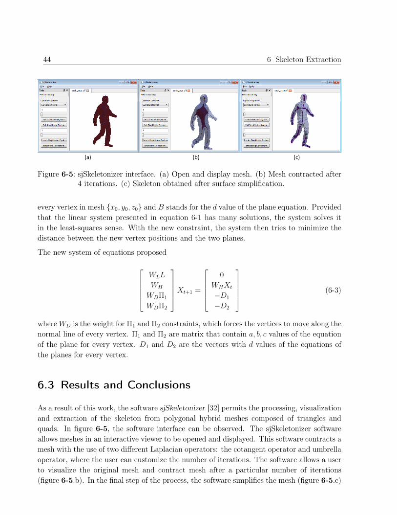
44 6 Skeleton Extraction
(a) (b) (c)
Figure 6-5: sjSkeletonizer interface. (a) Open and display mesh. (b) Mesh contracted after4 iterations. (c) Skeleton obtained after surface simplification.
every vertex in mesh x0, y0, z0 and B stands for the d value of the plane equation. Providedthat the linear system presented in equation 6-1 has many solutions, the system solves itin the least-squares sense. With the new constraint, the system then tries to minimize thedistance between the new vertex positions and the two planes.
The new system of equations proposed
WLL
WH
WDΠ1
WDΠ2
Xt+1 =
0
WHXt
−D1
−D2
(6-3)
whereWD is the weight for Π1 and Π2 constraints, which forces the vertices to move along thenormal line of every vertex. Π1 and Π2 are matrix that contain a, b, c values of the equationof the plane for every vertex. D1 and D2 are the vectors with d values of the equations ofthe planes for every vertex.
6.3 Results and Conclusions
As a result of this work, the software sjSkeletonizer [32] permits the processing, visualizationand extraction of the skeleton from polygonal hybrid meshes composed of triangles andquads. In figure 6-5, the software interface can be observed. The sjSkeletonizer softwareallows meshes in an interactive viewer to be opened and displayed. This software contracts amesh with the use of two different Laplacian operators: the cotangent operator and umbrellaoperator, where the user can customize the number of iterations. The software allows a userto visualize the original mesh and contract mesh after a particular number of iterations(figure 6-5.b). In the final step of the process, the software simplifies the mesh (figure 6-5.c)

6.3 Results and Conclusions 45
(a) (b) (c) (d)
Figure 6-7: Skeleton extracted from different models. (a) Dog model (b) Character model.(c) Person model. (d) Clay model.
using the same method proposed by Au et al. [3] that consists of a modified version ofquadric error metrics by Garland et al. [18] .
Figure 6-6: Model with different poses and skeleton obtained with our skeleton extractionsoftware.
Figure 6-7 shows the skeleton extracted from different models using our method. Everyskeleton accurately represents the topology and geometry of the original meshes. The ex-tracted skeletons are homotopic to the original shapes. Our method also allows the skeletonto be simplified to the user’s requirement in order to guarantee that every node in theskeleton closely represents every core part of the original model.
The method proposed is robust under isometric transformations ( figure 6-6) so that ifsome global transformations, such as rotations of central parts of the mesh, are made, theextracted skeletons will be similar because the Laplacian operator properties are invariantunder rotations. The figure shows similar skeletons for different poses of the same model,these skeletons show identical branching structure.

7 Conclusion
This work presented a novel extension of the Laplace Beltrami operator for hybrid quad/trianglemeshes, and the successful application of such principles in different types of problems incomputer geometric modelling like smoothing, enhancing, sculpting, deformation, reposingand skeleton extraction.
We have largely demonstrated that our method has good performance, stability and ro-bustness of the extension proposed. This novel extension of the Laplace Beltrami operatorwas introduced in the computer modeling industry inside the Blender 3D computer graphicssoftware, in order to facilitate artists who work with different tools developed using TQLBO,for any kinds of meshes, i.e., triangular meshes, quadrilateral meshes or hybrid meshes.

Bibliography
[1] Marc Alexa and Max Wardetzky. Discrete laplacians on general polygonal meshes. ACMTrans. Graph., 30(4):102:1–102:10, July 2011.
[2] D. Attali, J.-D. Boissonnat, and H. Edelsbrunner. Stability and computation of themedial axis — a state-of-the-art report. Mathematical Foundations of Scientific Visu-alization, Computer Graphics, and Massive Data Exploration, 1:–, 2007.
[3] Oscar Kin-Chung Au, Chiew-Lan Tai, Hung-Kuo Chu, Daniel Cohen-Or, and Tong-Yee Lee. Skeleton extraction by mesh contraction. ACM Transactions on Graphics,27(3):10, 2008.
[4] Mikhail Belkin, Jian Sun, and Yusu Wang. Discrete laplace operator on meshed surfaces.In Proceedings of the twenty-fourth annual symposium on Computational geometry, SCG’08, pages 278–287, New York, NY, USA, 2008. ACM.
[5] Henning Biermann, Adi Levin, and Denis Zorin. Piecewise smooth subdivision surfaceswith normal control. In Proceedings of the 27th annual conference on Computer graphicsand interactive techniques, SIGGRAPH ’00, pages 113–120, New York, NY, USA, 2000.ACM Press/Addison-Wesley Publishing Co.
[6] Blender-Foundation. Blender open source 3d application for modeling, animation, ren-dering, compositing, video editing and game creation. http://www.blender.org/, 2012.
[7] Mario Botsch, Mark Pauly, Christian Rossl, Stephan Bischoff, and Leif Kobbelt. Geo-metric modeling based on triangle meshes. In ACM SIGGRAPH 2006 Courses, SIG-GRAPH ’06, New York, NY, USA, 2006. ACM.
[8] Luc Buatois, Guillaume Caumon, and Bruno Lévy. Concurrent number cruncher: anefficient sparse linear solver on the gpu. In Proceedings of the Third international confer-ence on High Performance Computing and Communications, HPCC’07, pages 358–371,Berlin, Heidelberg, 2007. Springer-Verlag.
[9] E. Catmull and J. Clark. Recursively generated b-spline surfaces on arbitrary topologicalmeshes. Computer-Aided Design, 10(6):350–355, November 1978.
[10] Yong Chen and Charlie C. L. Wang. Uniform offsetting of polygonal model based onlayered depth-normal images. Comput. Aided Des., 43(1):31–46, January 2011.
[11] Sabine Coquillart. Extended free-form deformation: a sculpturing tool for 3d geometricmodeling. SIGGRAPH Comput. Graph., 24(4):187–196, September 1990.

48 Bibliography
[12] Nicu D. Cornea and Patrick Min. Curve-skeleton properties, applications, and algo-rithms. IEEE Transactions on Visualization and Computer Graphics, 13(3):530–548,2007.
[13] Tony DeRose, Michael Kass, and Tien Truong. Subdivision surfaces in character anima-tion. In Proceedings of the 25th annual conference on Computer graphics and interactivetechniques, SIGGRAPH ’98, pages 85–94, New York, NY, USA, 1998. ACM.
[14] Mathieu Desbrun, Mark Meyer, Peter Schröder, and Alan H. Barr. Implicit fairing ofirregular meshes using diffusion and curvature flow. In SIGGRAPH ’99: Proceedingsof the 26th annual conference on Computer graphics and interactive techniques, pages317–324, New York, NY, USA, 1999. ACM Press/Addison-Wesley Publishing Co.
[15] Mathieu Desbrun, Mark Meyer, Peter Schröder, and Alan H. Barr. Anisotropic feature-preserving denoising of height fields and bivariate data. In In Graphics Interface, pages145–152, 2000.
[16] Ran Gal, Olga Sorkine, Niloy J. Mitra, and Daniel Cohen-Or. iwires: An analyze-and-edit approach to shape manipulation. ACM Transactions on Graphics (Siggraph),28(3):#33, 1–10, 2009.
[17] Tinsley A. Galyean and John F. Hughes. Sculpting: an interactive volumetric modelingtechnique. SIGGRAPH Comput. Graph., 25(4):267–274, July 1991.
[18] Michael Garland and Paul S. Heckbert. Surface simplification using quadric error met-rics. In Proceedings of the 24th annual conference on Computer graphics and inter-active techniques, SIGGRAPH ’97, pages 209–216, New York, NY, USA, 1997. ACMPress/Addison-Wesley Publishing Co.
[19] Ozgur Gonen and Ergun Akleman. Smi 2012: Short paper: Sketch based 3d modelingwith curvature classification. Comput. Graph., 36(5):521–525, August 2012.
[20] Uwe Hahne. Weighting in Laplacian Mesh Editing. PhD thesis, Bauhaus-UniversitatWeimar, 2006.
[21] Takeo Igarashi, Satoshi Matsuoka, and Hidehiko Tanaka. Teddy: a sketching interfacefor 3d freeform design. In Proceedings of the 26th annual conference on Computergraphics and interactive techniques, SIGGRAPH ’99, pages 409–416, New York, NY,USA, 1999. ACM Press/Addison-Wesley Publishing Co.
[22] Bruno Levy. Numerical methods for digital geometry processing. In 2005 Israel-KoreaBi-national Conference on New Technologies and Visualization Methods for ProductDevelopment on Design and Reverse Engineering, Haifa/Israel, Nov 2005.
[23] Liu, L., Bajaj, C., Deasy, J. O., Low, D. A., Ju, and T. Surface reconstruction fromnon-parallel curve networks. Computer Graphics Forum, 27(2):155–163, April 2008.
[24] C. Loop. Smooth subdivision surfaces based on triangles. Department of mathematics,University of Utah, Utah, USA, August 1987.
Bibliography 49
[25] Mark Meyer, Mathieu Desbrun, Peter Schröder, and Alan H. Barr. Discrete differential-geometry operators for triangulated 2-manifolds. In Hans-Christian Hege and KonradPolthier, editors, Visualization and Mathematics III, pages 35–57. Springer-Verlag, Hei-delberg, 2003.
[26] Tony Mullen. Introducing character animation with Blender. Indianapolis, Ind. WileyPub. cop., 2007.
[27] Andrew Nealen, Takeo Igarashi, Olga Sorkine, and Marc Alexa. Laplacian mesh op-timization. In Proceedings of the 4th international conference on Computer graphicsand interactive techniques in Australasia and Southeast Asia, GRAPHITE ’06, pages381–389, New York, NY, USA, 2006. ACM.
[28] Yutaka Ohtake, Alexander Belyaev, and Hans-Peter Seidel. Ridge-valley lines on meshesvia implicit surface fitting. ACM Trans. Graph., 23(3):609–612, August 2004.
[29] Ulrich Pinkall, Strasse Des Juni, and Konrad Polthier. Computing discrete minimalsurfaces and their conjugates. Experimental Mathematics, 2:15–36, 1993.
[30] Alexander Pinzon, Fabio Martinez, and Eduardo Romero. Análisis experimental dela extracción del esqueleto por contracción con suavizado laplaciano, December 2010.Poster presented at 6th International Seminar on Medical Image Processing and Analy-sis (SIPAIM 2010), December 1–4, Universidad Nacional de Colombia, Bogota, Colom-bia.
[31] Alexander Pinzon and Eduardo Romero. Software para la extracción del esqueleto porcontracción y suavizado, December 2011. Poster presented at 7th International Seminaron Medical Image Processing and Analysis (SIPAIM 2011), December 6–8, UniversidadIndustrial de Santander, Bucaramanga, Colombia.
[32] Alexander Pinzon and Eduardo Romero. sjskeletonizer: Skeleton extraction software.,March 2012. http://code.google.com/p/jeronimo/.
[33] Alexander Pinzon and Eduardo Romero. Shape inflation with an adapted laplacian op-erator for hybrid quad/triangle meshes. 2013 26th SIBGRAPI Conference on Graphics,Patterns and Images, 0:179–186, 2013.
[34] Pawas Ranjan. Discrete Laplace Operator: Theory and Applications. PhD thesis, TheOhio State University, Columbus, OH, USA, 2012.
[35] Steven Rosenberg. The Laplacian on a Riemannian manifold: an introduction to anal-ysis on manifolds. Number 31. Cambridge University Press, 1997.
[36] Robert Schneider, Leif Kobbelt, and Hans-Peter Seidel. Improved bi-laplacian meshfairing. In Tom Lyche and Larry L. Schumaker, editors, Mathematical Methods forCurves and Surfaces: Oslo 2000, Innovations in Applied Mathematics, pages 445–454,Oslo, Norway, 2001. Vanderbilt University.
50 Bibliography
[37] O. Sorkine, D. Cohen-Or, Y. Lipman, M. Alexa, C. Rössl, and H.-P. Seidel. Laplaciansurface editing. In Proceedings of the 2004 Eurographics/ACM SIGGRAPH symposiumon Geometry processing, SGP ’04, pages 175–184, New York, NY, USA, 2004. ACM.
[38] Olga Sorkine. Differential representations for mesh processing. Comput. Graph. Forum,1:789–807, 2006.
[39] Michael Spivak. A Comprehensive Introduction to Differential Geometry, volume 1.Publish or Perish, Inc, 3rd edition, January 1999.
[40] Jos Stam. Exact evaluation of catmull-clark subdivision surfaces at arbitrary param-eter values. In Proceedings of the 25th annual conference on Computer graphics andinteractive techniques, SIGGRAPH ’98, pages 395–404, New York, NY, USA, 1998.ACM.
[41] Lucian Stanculescu, Raphalle Chaine, and Marie-Paule Cani. Freestyle: Sculptingmeshes with self-adaptive topology. Computers & Graphics, 35(3):614 – 622, 2011.Shape Modeling International (SMI) Conference 2011.
[42] Gabriel Taubin. A signal processing approach to fair surface design. In Proceedings of the22nd annual conference on Computer graphics and interactive techniques, SIGGRAPH’95, pages 351–358, New York, NY, USA, 1995. ACM.
[43] Yunhui Xiong, Guiqing Li, and Guoqiang Han. Mean laplace-beltrami operator forquadrilateral meshes. In Zhigeng Pan, Adrian Cheok, Wolfgang Muller, and Xubo Yang,editors, Transactions on Edutainment V, volume 6530 of Lecture Notes in ComputerScience, pages 189–201. Springer Berlin / Heidelberg, 2011.
[44] Guoliang Xu. Discrete laplace-beltrami operators and their convergence. Comput. AidedGeom. Des., 21(8):767–784, 2004.
[45] Kun Zhou, Jin Huang, John Snyder, Xinguo Liu, Hujun Bao, Baining Guo, and Heung-Yeung Shum. Large mesh deformation using the volumetric graph laplacian. ACMTrans. Graph., 24(3):496–503, July 2005.
[46] Wei Zhuo and Jarek Rossignac. Curvature-based offset distance: Implementations andapplications. Computers & Graphics, 36(5):445 – 454, 2012.