an adaptive gradient algorithm for maximum likelihood ... · an adaptive gradient algorithm for...
TRANSCRIPT

Gerhard Winkler:
An Adaptive Gradient Algorithm for MaximumLikelihood Estimation in Imaging: A Tutorial
Sonderforschungsbereich 386, Paper 120 (1998)
Online unter: http://epub.ub.uni-muenchen.de/
Projektpartner
An Adaptive Gradient Algorithm
for Maximum Likelihood Estimation in Imaging�A Tutorial
Gerhard Winkler
Institute of Biomathematics and BiometryGSF � National Research Center for Environment and Health
D������ Neuherberg� Germanye�mail gwinkler�gsf�de
Keywords� adaptive algorithm� stochastic approximation� stochastic gradientdescent� MCMC methods� maximum likelihood� Gibbs �elds� imaging
Abstract
Markov random �elds serve as natural models for patterns or textures
with random �uctuations at small scale� Given a general form of such
�elds each class of pattern corresponds to a collection of model parameters
which critically determines the abilitity of algorithms to segment or clas�
sify� Statistical inference on parameters is based on �dependent� data given
by a portion of patterns inside some observation window� Unfortunately�
the corresponding maximum likelihood estimators are computationally in�
tractable by classical methods� Until recently� they even were regarded
as intractable at all� In recent years stochastic gradient algorithms for
their computation were proposed and studied� An attractive class of suchalgorithms are those derived from adaptive algorithms� wellknown in en�
geneering for a long time�
We derive convergence theorems following closely the lines proposed
by M� M�etivier and P� Priouret ����� This allows a transparent
�albeit somewhat technical� treatment� The results are weaker than those
obtained by L� Younes �����
� Introduction
Markov random �elds serve as �exible models in image analysis� speech recogni�tion and many other �elds� In particular� textures with random �uctuations atsmall scale are reasonably described by random �elds� A large class of recursiveneural networks can be reinterpreted in this framework as well�
Let a pattern be represented by a �nite rectangular array x � xss�S of�greyvalues� or �colours� xs � Gs in �pixels� s � S where all sets Gs and S are�nite� A �nite random eld is a strictly positive probability measure on the
� INTRODUCTION �
�nite space X �Qs�S Gs of all con�gurations x� Taking logarithms shows that
is of the Gibbsian form
x � Z�� exp�Kx� Z �Xz
exp�Kz� �
with an energy function K on X� �Modelling� a certain type of pattern or textureamounts to the choice of a random �eld� typical samples of which share su��ciently many statistical properties with samples from the real pattern� Hence thechoice of K usually is based on statistical inference besides prior knowledge� Anonparametric approach is not feasible and we restrict attention to the linearparametric case� We consider families
� � f ��� � � � �g �
of random �elds onX� where � � Rd is the parameter space and each distribution
is a Gibbs �eld of the exponential form
��� � Z��� exp h��Hi � � � ��
The energy is given by K� � �h��Hi where H � H�� � � � � Hd is a vector offunctions on X� � � � � R
d� and h��Hi is the Euclidean inner product�Given a sample x � X� a maximum likelihood estimator ��x maximizes the
�log�� likelihood function
Lx� � � � �� R� � ��� ln x���
The covariance of Hi and Hj under ��� will be denoted by covHi� Hj��and the corresponding covariance matrix by covH��� Straightforward calcula�tions give ����� Prop� ������
Proposition ��� Let � be open The likelihood function � �� Lx�� is innitelyoften continuously di�erentiable for every x The gradient is given by
�
��iLx�� � Hix� E Hi�� �
and the Hessean matrix is given by
��
��i��jLx�� � �cov Hi� Hj�� �
In particular� the likelihood function is concave
This result tells us that direct computation of ML estimators in the presentcontext is not possible� In fact� the expectation in the gradient is a sum overX which may have cardinality of order ����������� Because of the mentioned
� INTRODUCTION �
misgivings� ML estimators on large spaces until recently were thought to becomputationally intractable� Therefore� J� Besag in ���� ��� suggested the codingand the pseudo�likelihood method where the full likelihood function is replacedby �pseudo�likelihoods� based on conditional probabilities only� These estimatorsare computationally feasible in many cases cf� ���� and also ����
In the last decade� accompanied by the development of learning algorithmsfor Neural Networks and encouraged by the increase of computer power� recursivealgorithms for the computation or at least apprioximation of maximum likelihoodestimators themselves were studied� Many of them are related to basic gradientascent which is ill�famed for poor convergence� More sophisticated methodsfrom numerical analysis violate the requirement of �locality� which basically meansthat the updates can be computed component by component from the respectivepreceding components� In this paper� we study the asymptotics of adaptivealgorithms which we hasten to de�ne now�
We want to compute maximum likelihood estimators for Gibbs �elds� i�e�maximize the likelihood function W � Lx� � for a �xed sample x � X� Thestarting point is steepest ascent
��k��� � ��k� � �k��rW ��k� � ��k� � �k���Hx� EH���k�
��
with gains �k possibly varying in time� Given ���� � Rd� the adaptive algorithm
is recursively de�ned by
��k��� � ��k� � �k�� Hx�H�k��
P �k�� � z j�k � x � Pkx� z �
where Pk is the Markov kernel of one sweep of the Gibbs sampler for ����k��The Gibbs sampler is a Markov process on X which via a law of large numbersgives estimates of the expectations appearing in �� It will be de�ned below�Note that �k� ��k�k�� is a Markov process taking values in X � R
d and livingon a suitable probability space ��F �P� We shall be mainly interested in themarginal process ��k�k���
Let us brie�y comment on the philosophy behind� Consider the ordinarydi�erential equation ODE
��t � rW �t� t � �� �� � ����� �
where �� � d�dt� Under mild assumptions on W � each of these initial valueproblems has a unique solution �tt�� and �t� �� as t� cf� Proposition
���� Hence a process���k�
�converges to �� if it stays near a solution� Steepest
ascent can be interpreted as an Euler method for the discrete approximation ofsolutions of the ODE� Similarly� the paths of � will be compared to the solutionsof ��
� THE GIBBS SAMPLER �
Coupling the Gibbs sampler and an ascent algorithm like in � amountsto adaptive algorithms which play an important role in �elds of engineering likesystem identi�cation� signal modelling� adaptive �ltering and others� They re�ceived considerable interest in recent years and were studied by M�etivier andPriouret �� !� ����� in a general framework� The circle of such ideas is illus�trated� surveyed and extended in the monograph Benveniste� M�etivier andPriouret ����� ���� an extended English version of the French predecessor from�� !� The monograph Freidlin and Wentzell �� �� ���� had considerablein�uence on the development of the theory�
The theory of adaptive algorithms was applied to ML estimation in imagingby L� Younes �� � �� �� ����� ��!�� �� �� In some respects� the theorygets simpler in this setting due to the boundedness of the energy function K�On the other hand� some assumptions from the general theory are not met andtherefore additional estimates are required� Younes �� � ��!�� proves almostsure convergence developing a heavy technical machinery� We decided to steera middle course� we shall follow the lines of M�etivier� Priouret �� !� �����closely in order not to obscure the main ideas by too many technical details� Onthe other hand the results will be weaker than Younes��
The reader we have in mind should be acquainted with general probabilityspaces and conditional expectations� He or she should also have met discrete�time�continuous�space Markov processes and martingales� Concerning martingale the�ory� part of the six pages ����� pp� ����!� is su�cient� For more backgroundinformation the reader may consult ���� and �!��
� The Gibbs Sampler
To complete the de�nition of the algorithm � the Gibbs sampler is introducednow� Let be a Gibbs �eld of the form � and consider the Markov chainrecursively de�ned by the rules�
�� Enumerate the sites in S� i�e� let S � f�� � � � � jSjg��� Choose an initial con�guration x��� � X�
�� Given x�k�� pick a greyvalue y� � G� at random from X� � �jXj �
x�k�j � j � �� Given the con�guration updated in the last pixel repeat this
step for s � �� � � � � jSj� Now a �sweep� is �nished with the result x�k����
The symbol jSj denotes the number of elements in S� the enumeration of Sis called a deterministic visiting scheme� the projections X � Gj� x �� xj aredenoted by Xj and AjB is the conditional probability of A given B� Formally�the Gibbs sampler is a homogeneous Markov chain with transition probability
P x� y � � � � � jSj�
� MAIN RESULTS �
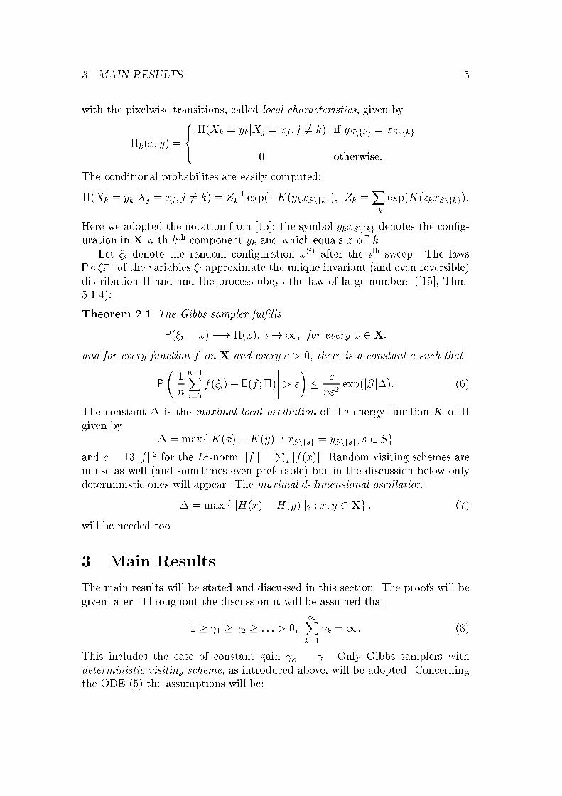
with the pixelwise transitions� called local characteristics� given by
kx� y �
�����
Xk � ykjXj � xj� j � k if ySnfkg � xSnfkg
� otherwise�
The conditional probabilites are easily computed�
Xk � ykjXj � xj� j � k � Z��k exp�KykxSnfkg� Zk �
Xzk
expKzkxSnfkg�
Here we adopted the notation from ����� the symbol ykxSnfkg denotes the con�g�uration in X with kth component yk and which equals x o� k�
Let �i denote the random con�guration x�i� after the ith sweep� The lawsP � ���i of the variables �i approximate the unique invariant and even reversibledistribution and and the process obeys the law of large numbers ����� Thm�������
Theorem ��� The Gibbs sampler fullls
P�i � x �� x� i�� for every x � X�
and for every function f on X and every � �� there is a constant c such that
P
��nn��Xi�
f�i� Ef �
�
� c
n�expjSj"� �
The constant " is the maximal local oscillation of the energy function K of given by
" � maxfjKx�Kyj � xSnfsg � ySnfsg� s � Sgand c � ��kfk� for the L��norm kfk �
Px jfxj� Random visiting schemes are
in use as well and sometimes even preferable but in the discussion below onlydeterministic ones will appear� The maximal d�dimensional oscillation
#" � max fkHx�Hyk� � x� y � Xg � !
will be needed too�
� Main Results
The main results will be stated and discussed in this section� The proofs will begiven later� Throughout the discussion it will be assumed that
� � �� � �� � � � � � ���Xk�
�k ��
This includes the case of constant gain �k � �� Only Gibbs samplers withdeterministic visiting scheme� as introduced above� will be adopted� Concerningthe ODE � the assumptions will be�
� MAIN RESULTS �
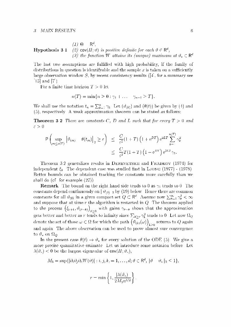
Hypothesis ������ � � R
d���� covH�� is positive denite for each � � R
d���� the function W attains its �unique� maximum at �� � R
d
The last two assumptions are ful�lled with high probability� if the family ofdistributions in question is identifyable and the sample x is taken on a su�cientlylarge observation window S� by recent consistency results ���� for a summary see���� and �!��
For a �nite time horizon T � � let
nT � minfn � � � �� � � � �� �n�� � Tg�We shall use the notation tn �
Pnk� �k� Let ��k� and �t be given by � and
�� respectively� A weak approximation theorem can be stated as follows�
Theorem ��� There are constants C� D and L such that for every T � � and � �
P
�sup
m�n�T �
�����m� � �tm�����
� C
�� � T
�� � eDT
�e�LT
n�T �Xk�
��k
� C
�T � � T
�� � eDT
�e�LT���
Theorem ��� generalizes results in Derevetskii and Fradkov ��!� forindependent �k� The dependent case was studied �rst in Ljung ��!! � ��! �Better bounds can be obtained tracking the constants more carefully than weshall do cf� for example �!�
Remark� The bound on the right hand side tends to � as �� tends to �� Theconstants depend continuously on k����k� by �� below� Hence there are commonconstants for all ���� in a given compact set Q � R
d� Assume nowP�
k� ��k �
and suppose that at time r the algorithm is restarted in Q� The theorem appliedto the process
��r�k� ��r�k�
�k��
with gains �r�k shows that the approximation
gets better and better as r tends to in�nity sinceP
k�r ��k tends to �� Let now �Q
denote the set of those � � for which the path���k�
�k��
returns to Q again
and again� The above observation can be used to prove almost sure convergenceto �� on �Q�
In the present case �t � �� for every solution of the ODE �� We give amore precise quantitative estimate� Let us introduce some notation before� Let��� � � be the largest eigenvalue of covH����
M � supfj�i�j�kW �j � i� j� k�� �� � � � � d�� � Rd� k�� ��k� � �g�
r � min
���
j���j�Mn���
�

� MAIN RESULTS !
and �nally�� � inffkrW �k�� � k�� ��k�� � �g�
Then
Lemma ��� Each initial value problem ��� has a unique solution �tt�� and�t� �� as t� Moreover�
k�t� ��k� � r exp
��j���j
�t� �
for t � �
where � � jW ���W ��j�r All this is proved in the Appendix� By these results the following makes sense�
Corollary ��� Given � � choose T � � such that k�T � ��k� � Then
P
������n�T �� � ������� �
�� C��� T
where C��� T � � as �� � �
For special choices of gains almost sure convergence holds�
Theorem ��� Younes ����� Let �k � uk��� u � �� #"� Then
��n� �� �� P� almost everywhere�
As already mentioned� the proof of this strong result is fairly technical and willnot be given here� Nevertheless� the main idea is similar to that presented below�
The following informal argument might nourish the hope that the programcan be carried out� We know that the Gibbs sampler as a time�homogeneousMarkov process obeys the law of large numbers� i�e means w�r�t� ��� can beapproximated by means in time cf� Theorem ���� Let � � � be a constant gain�Choose r � � and n � �� Then
��r�n� � ��r� � �n��Xk�
Hx�H�r�k��
� ��n� � n�
�Hx� �
n
n��Xk�
H �r�k��
��r� � n�rW ��r��
The approximation holds if �r�kn��k� is approximately stationary and n is large�
For the former� the parameters ��r�k� should vary rather slowly which is the casefor small gain and small n� The proper balance between the requirements �nsmall� and �n large� is one of the main problems in the proof�
� ERROR DECOMPOSITION AND L��ESTIMATES
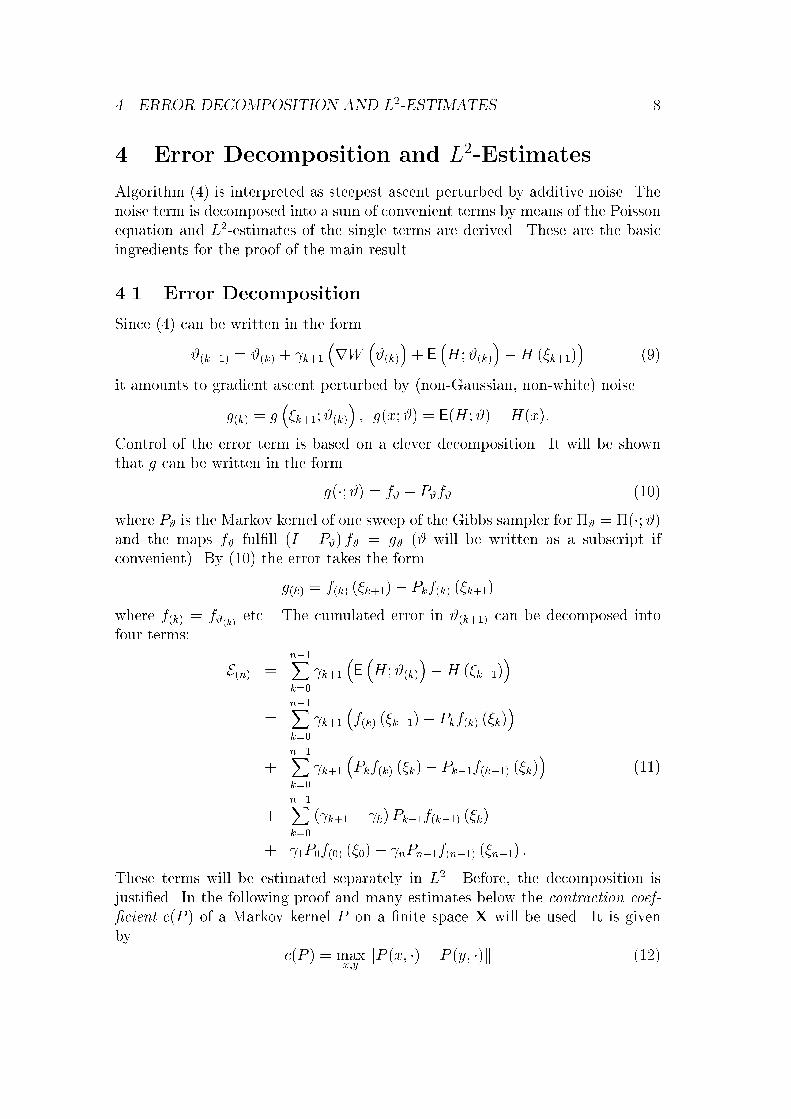
� Error Decomposition and L��Estimates
Algorithm � is interpreted as steepest ascent perturbed by additive noise� Thenoise term is decomposed into a sum of convenient terms by means of the Poissonequation and L��estimates of the single terms are derived� These are the basicingredients for the proof of the main result�
��� Error Decomposition
Since � can be written in the form
��k��� � ��k� � �k��
�rW
���k�
�� E
�H���k�
��H �k��
��
it amounts to gradient ascent perturbed by non�Gaussian� non�white noise
g�k� � g��k�����k�
�� gx�� � EH���Hx�
Control of the error term is based on a clever decomposition� It will be shownthat g can be written in the form
g��� � f� � P�f� ��
where P� is the Markov kernel of one sweep of the Gibbs sampler for � � ���and the maps f� ful�ll I � P� f� � g� � will be written as a subscript ifconvenient� By �� the error takes the form
g�k� � f�k� �k��� Pkf�k� �k��
where f�k� � f��k� etc�� The cumulated error in ��k��� can be decomposed intofour terms�
E�n� �n��Xk�
�k��
�E
�H���k�
��H �k��
�
�n��Xk�
�k��
�f�k� �k��� Pkf�k� �k
�
�n��Xk�
�k��
�Pkf�k� �k� Pk��f�k��� �k
���
�n��Xk�
�k�� � �kPk��f�k��� �k
� ��P�f��� ��� �nPn��f�n��� �n�� �
These terms will be estimated separately in L�� Before� the decomposition isjusti�ed� In the following proof and many estimates below the contraction coef�cient cP of a Markov kernel P on a �nite space X will be used� It is givenby
cP � maxx�y
kP x� �� P y� �k ��
� ERROR DECOMPOSITION AND L��ESTIMATES �
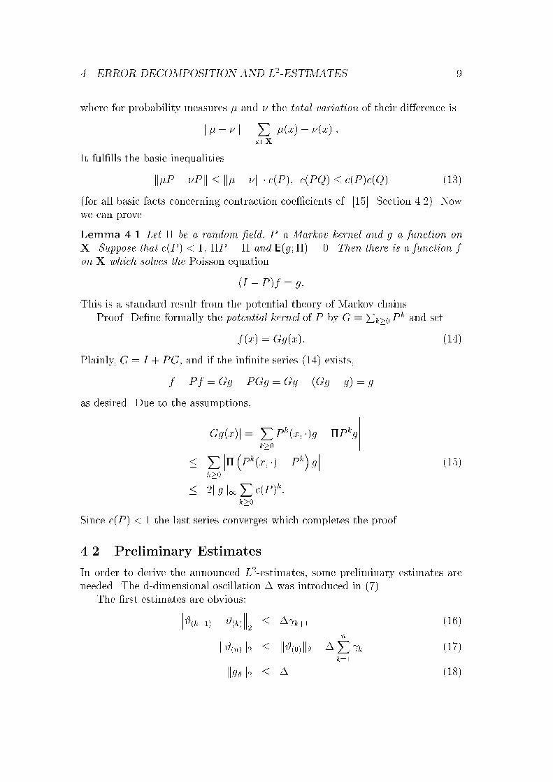
where for probability measures � and � the total variation of their di�erence is
k�� �k �Xx�X
j�x� �xj�
It ful�lls the basic inequalities
k�P � �Pk � k�� �k � cP � cPQ � cP cQ ��
for all basic facts concerning contraction coe�cients cf� ����� Section ���� Nowwe can prove
Lemma ��� Let be a random eld� P a Markov kernel and g a function onX Suppose that cP � �� P � and Eg� � � Then there is a function fon X which solves the Poisson equation
I � P f � g�
This is a standard result from the potential theory of Markov chains�Proof� De�ne formally the potential kernel of P by G �
Pk�� P
k and set
fx � Ggx� ��
Plainly� G � I � PG� and if the in�nite series �� exists�
f � Pf � Gg � PGg � Gg � Gg � g � g
as desired� Due to the assumptions�
jGgxj �Xk��
P kx� �g � P kg
� X
k��
�P kx� �� P k�g ��
� �kgk�Xk��
cP k�
Since cP � � the last series converges which completes the proof�
��� Preliminary Estimates
In order to derive the announced L��estimates� some preliminary estimates areneeded� The d�dimensional oscillation #" was introduced in !�
The �rst estimates are obvious������k��� � ��k������ #"�k�� ��
k��n�k� � k����k� � #"nX
k�
�k �!
kg�k� � #" �
� ERROR DECOMPOSITION AND L��ESTIMATES ��
It is easily seen that cP� � ��exp� #"k�k� ����� ���� and hence by �!�
�� cPk�� � exp
�� #"k����k�
�exp
�� #"�tk
�� C expDtk� ��
The following estimates are less obvious�
Lemma ��� There are constants C and D such that���f�k������ C expDtk �����Pk��f�k��� � Pkf�k�
����� C expDtk��
�����k��� � ��k�����
��
Proof� By �� and � �
kf�k� � � #"�� cP����
Hence �� implieskf�k�k� � � #"C expDtk�
The proof of �� is technical and lengthy and hence will be postponed to Section�� Lemma ���� For the moment� take it for granted�
Let us �nally note the simple but useful relation
������pX
j�
aj�j
�������
�
��� pXj�
aj
�A pX
j�
aj k�jk�� ��
for aj � � and �j � Rd� If all aj vanish there is nothing to show� otherwise it
amounts to a modi�ed de�nition of convexity�
��� L��Estimates
L��estimates for the four sums in �� will be derived now� The �rst one is mostinteresting� Set
S�n� �n��Xk�
�k��
�f�k� �k��� Pkf�k� �k
��
Lemma ��� There are constants C and D such that
E
�maxm�n
���S�m�
�k���� C
n��Xk�
expDtk��k���
Proof� First we shall show that S ��S�n�
�n��
is a martingale� To this end�
let Fn denote the ���eld generated by ��� � � � � �n� Note that ����� � � � � ��n� areFn�measurable as well� By construction of the process�
E
�f�k� �k�� jFk
�� Pkf�k� �k �
� ERROR DECOMPOSITION AND L��ESTIMATES ��
Hence the term in S�n� with index k � n � � vanishes conditioned on Fn� Theother summands are Fn�measurable and hence invariant under conditioning� Thisproves the martingale property
E
�S�n� jFn
�� S�n����
By Jensen�s inequality�
E
����f�k� �k�������
�� E
�E
����f�k� �k�������jFk
��
� E
�E
����f�k� �k������jFk
���� E
����Pkf�k� �k�����
��
By orthogonality of increments ����� Lemma ������
E
�S�n���� E
�n��Xk�
��k�����f�k��k��� Pkf�k��k
�����
�
By ��� the previous estimate� and ��� one may proceed with
E
�kS�n�k��
�� �E
�n��Xk�
��k��kf�k���k���k��� �C
n��Xk�
��k�� exp�Dtk�
The uniform estimate in m � n �nally follows from Doob�s L��inequality �����Lemma ������
E
�maxm�n
kS�m�k���� �E
�kS�n�k��
��
This completes the proof�The remaining three estimates are straightforward�
Lemma ��� There are constants C and D such that
ak �����k��
�Pkf�k��k� Pk��fk���k
������ C expDtk�
�k
bk �����k�� � �kPk��f�k����k
����� C expDtk���k�� � �k
ck ������P�f������ �nPn��f�n����n��
����� C exp�Dtn��
���n � ���
�
Proof� By �� and �!�
����k��Pkf�k��k� Pk��f�k����k����
� �k��Ck��k� � ��k���k� expDtk � C ���k expDtk
which proves the �rst estimate� The second one follows from ��� The third oneis implied by �� and �� with p � �� aj � ��
Now we can put things together to derive the L��estimate of the total error�
� PROOF OF THE APPROXIMATION THEOREM ��
Proposition ��� There are constants C and D such that
E
�maxm�n
kE�m�k���� C expDtn��
�� �
nXk�
��k
�nX
k�
��k
�
Proof� We shall use �� and Lemmata ��� and ���� By �� for p � � and aj � ��
E
�maxm�n
kE�m�k���
� �
��E�max
m�nkS�m�k��
��
�n��Xk�
ak
�
�
�n��Xk�
bk
�
� cn
�A �
Plainly�
�n��Xk�
ak
�
� C
�n��Xk�
��k expDtk
�
� exp�Dtn��
�n��Xk�
��k
�n��Xk�
bk
�
� C
�n��Xk�
�k�� � �k expDtk��
�
� C exp�Dtn���n � ��� � C exp�Dtn���
�� �
Summation now gives the desired result�For a �nite time horizon the estimate boils down to
Corollary �� There are constants C and D such that for every T � ��
E
�max
m�n�T �kE�m�k��
� CeDT � � ��T
n�T �Xk�
��k�
� Proof of the Approximation Theorem
We complete now the proof of Theorem ��� and append the missing estimates�The main tool is the following discrete Gronwall lemma�
Lemma ��� If the real sequence bkk�� satises
b� � �� br � C �DrX
k�
�kbk�� for r � �� � � � � n�
with C�D � � then
bn � C exp
�D
nXk�
�k
�

� PROOF OF THE APPROXIMATION THEOREM ��
Proof� If C or D vanishes there is nothing to show� Hence we may assume thatD � � otherwise we modify the �k� First we show
� �rX
k�
�k exp
��k��Xj�
�j
�A � exp
�rX
k�
�k
� r � �� � � � � n� ��
For r � � this boils down to ���� � exp�� which plainly is true� The inductionstep reads
exp
�r��Xk�
�k
� exp
�rX
k�
�k
exp�r��
� exp
�rX
k�
�k
� �r�� exp
�rX
k�
�k
� � �
�� rXk�
�k exp
��k��Xj�
�j
�A�A� �r�� exp
�rX
k�
�k
� � �
��r��Xk�
�k exp
��k��Xj�
�j
�A�A �
The �rst inequality follows from expx � � � x and the second one from theinduction hypothesis�
Since b� � C the assertion holds for r � �� If it holds for all k � r then using��� the assumption and the induction hypothesis
br�� � C
��� � r��X
k�
�k exp
��k��Xj�
�j
�A�A � C exp
�r��Xk�
�k
and the desired inequality is veri�ed�Solutions of the ODE � and steepest ascent will be compared now� Since
jHi � EHij � #"
the following estimates hold�
krW �k� � #"� jcov�Hi� Hjj � #"�� ��
For a smooth map t �� �t the chain rule reads
d
dt
�
��iW �t �
dXj�
��
��i��jW �t
d
dt�jt� ��
This will be used to prove�

� PROOF OF THE APPROXIMATION THEOREM ��
Lemma ��� There are a constant C and maps ��k� such that
�tk��� �tk � �k��rW �tk � ��k�
k��k�k� � C��k���
Proof� If �t solves � then
�tk��� �tk �Z tk��
tkrW �t dt� ��
By the mean value theorem
�
��iW �t �
�
��iW �tk �
d
dt
�
��iW �sitt� tk
for some sit � �tk� t�� By �� applied to t �� �t and since ��t � rW �tthe identity holds with
��k��i �Z dX
j�
��
�i�jW �sitrW sitt� tk dt�
Since jt� tkj � �k�� if tk � t �k�� and by ���
j��k��ij � d #"��k��
which implies the inequality�These and the previous L��estimates are combined with the Gronwall lemma
to prove the main result�Proof of Theorem ���� Let �tt�� be a solution of �� By � and Lemma
����
��k� � ��k��� � �krW ��k��� � �kg�k���
�tk � �t�k��� � �krW �tk�� � ��k����
Hence
��n� � �tn �n��Xk�
�k��rW ��k��rW �tk � E�n� �n��Xk�
��k��
By Lemmata ��� and ����
k��n� � �tnk� � Ln��Xk�
�k��k��k� � �tkk� � kE�n�k� � Cn��Xk�
��k��
��kE�n�k� � C
n��Xk�
��k��
exp
�L
nXk�
�k
�
� PROOF OF THE APPROXIMATION THEOREM ��
If tn � T then
k��n� � �tnk�� � �
��kE�n�k�� � C�
�n��Xk�
��k��
��A exp�LT �
By ��� ��n�T �X
k�
��k
�A�
�n�T �Xk�
�k
n�T �Xk�
�k � ��Tn�T �Xk�
��k�
Together with Proposition ��� this implies
E
�max
m�n�T �k��m� � �tmk��
� f�C expDT ����T ��C���Tg exp�LT
n�T �Xk�
��k�
Since �� � � the last quantity is dominated by an expression of the form
C� � T � � expDT exp�LT n�T �Xk�
��k� �!
Application of Markov�s inequality now completes the proof�Finally� the estimate �� is veri�ed�
Lemma ��� There are constants C and D such that ���j f��i � C exp�Dk�k�
kPk��f�k��� � Pkf�k�k� � C exp�Dtk��k��k��� � ��k�k��Proof� Existence of partial derivatives and the �rst estimate will be proved si�multaneously� By ��� f� �
Pk�� P
k�g�� Since
E�g� � �� �Pk�g�� �
one has
f�x �Xk��
Xx��y
�x��P k� x� y� P k
� x�� y
�giy ��
Xk��
S�k�� x�
Since � and k will be �xed for a while� they will be dropped�� The chain rule gives
�
��jS�k�i �
Xx��y
�
��j x�
�P kx� y� P kx�� y
�giy
�Xx��y
x�
��
��jP kx� y� �
��jP kx�� y
giy
�Xx��y
x��P kx� y� P kx�� y
� �
��jgiy
� � R��� �R��� �R��� ��
� PROOF OF THE APPROXIMATION THEOREM ��
It is easy to see that R���� R��
� � #"� � LcP k� ��
in fact��
��j x� � x� ln x�
and hence by Proposition ���� ���j x�
� #"
which proves the estimate of R���� Concerning R�� use Proposition ��� and ���� Estimating R��� is cumbersome and tricky� First the partial derivatives
have to be computed� For s � S and x� y � X the local characteristic is given by
fsgx� z � �xSnfsgzSnfsgz zsjzSnfsg�Proposition ��� for conditional Gibbs �elds yields
�
��j �zsjzSnfsg
��
��
��jln zsjzSnfsg
zsjzSnfsg
� Hjz� EHjjzSnfsg szsjzSnfsg� � �sz zsjzSnfsg ��
which implies�
��j fsgx� z � �sz fsgx� z�
In one sweep z � X is reached from x with positive probability along preciselyone path z� � x� z�� � � � � z� � z and hence
P x� z ��Y
s�
fsgzs��� zs
where it is tacitly assumed that S � f�� � � � � �g and that the sites are visited inincreasing order� By the product rule
�
��jP x� z � P x� z
�Xs�
�szs �� P x� z�x� z
wherej�x� zj � � #"� ��
Repeating this argument for
P kx� y �X
z������zk��
P x� z� � � � � � P zk��� y� k � ��
� PROOF OF THE APPROXIMATION THEOREM �!
gives�
��jP kx� y �
Xz������zk��
kXr�
�zr��� zrP x� z� � � � � � P z���� y
where z� � x and z� � y� Rearranging summation gives
�
��jP kx� y �
kXr�
Xu�v
�u� vP u� vP r��x� uP k�rv� y� ��
� Plugging �� into R��� results in
R��� �kX
r�
Xx��u�v
x��P r��x� u� P r��x�� u
�P u� v�u� v�X
y
P r�kv� ygiy�
By � the last sumP
y � � � can be replaced byXw�y
w�P k�rv� y� P k�rw� y
�giy
which can be estimated by �kgik�cP k��� Similarly� the remaining term isbounded by �� #"kcP r��� In summary�R���
� CkcP k��� ��
Note �nally that R��� � � if k � ��� Putting ��� �� and �� together yields
�Xk�
�
��jS�k���i
� C
��Xk�
cP�k �
�Xk�
k � �cP�k
� C��� cP�
�� � �� cP����
� �C �� cP��� � �C exp �Dk�k�
where �� was used in the last line� This shows that derivatives of partial sumsconverge uniformly on every compact subset of Rd� hence di�erentiation andsummation may be interchanged and the �rst inequality holds�
� For the second inequality� use the triangle inequality���Pn��f�n���y� Pnf�n�y���
����Pn�� � Pn f�n���y
��������Pn �f�n��� � f�n�
�y����
� � A �B�
Setting �s � ��n� � s���n��� � ��n�
�� �� implies
jPn��x� y� Pnx� yj �Z �
�
d
dtP��s�x� y ds
�
Z �
�h��n��� � ��n��rP��s�x� yi ds
� �����n��� � ��n�����
pd� #"�
� APPENDIX� HOW CLOSE IS �T TO �� �
Hence by ���
A � C exp Dtn�����n��� � ��n�
�����
By �!� both ��n� and ��n��� are contained in a ball B of radius C � � #"tn��
around � � Rd and by convexity �s� s � ��� �� as well� Hence the �rst inequality
implies
B �����f�n��� � f�n�
�y�����Z �
�h��n��� � ��n��rf��s� ds
�
�����n��� � ��n�����C exp �Dtn�� �
The estimates of A and B imply the second inequality�
� Appendix� How Close is ��t� to ��
It is shown now that each of the initial value problems � has a unique solutionand that each solution converges to the unique maximum likelihood estimator�Moreover estimates are given for the time one has to wait until a solution enters agiven neighbourhood of ��� This yields an estimate of the �nite time horizon T inTheorem ��� needed to guarantee a prescribed precision of the approximation of�� by the algorithm �� This appendix is included for convenience of the readeronly since all arguments are standard�
Let k � kM denote the matrix norm�
Proposition �� Each initial value problem ��� has a unique solution �t� t � ��and �t� �� as t�
Proof� By Proposition ���� the estimates �� and �� applied to the map �t �� � t�� � �� one has the estimate
����� ddtrW �t
������
� kcovH��tkMk ��tk� � d #"�k ��tk�� ��
Hence
krW ���rW �k� �Z �
�
����� ddtrW �t
������
dt � d #"�k�� � �k�
and thus the right hand side of � is Lipschitz continuous� In particular� eachinitial value problem � has a unique solution �t� t � �� Solutions of �converge to �� as t � which follows from elementary stability theory� Wehave
d
dtW � �t � �jrW �tj�
� APPENDIX� HOW CLOSE IS �T TO �� ��
by the chain rule and �� Hence W is a global Ljapunov function for the gradientsystem � and� moreover� �� is the only critical point� This completes the proof�
A rough estimate for the distance between the solution of the di�erentialequation � and the limit �� will be derived now� It will �rst be stated in ageneral form� Consider the gradient system
��t � �rV �t� �� � ��� ��
Throughout the discussion the following hypothesis will be assumed�
Hypothesis ����� V � CRn�R� V � � �� V � � � if � � � ��� The Hessean matrix C of V is positive denite at � � � ��� For each � � �� �� � inffkrV �k�� � k�k�� � �g � ��
Note that � � Rd now plays the role of �� in the previous discussion� Hence the
maximal solution � of �� is de�ned on ��� and �t� � as t�� Let
M � supnj�i�j�kV �j � i� j� k � �� � � � � d�� � R
d� k�k� � �o
and let �� denote the smallest eigenvalue of C�� By � in Hypothesis ���one has �� � �� Finally set
r � min
���
��
�Mn���
�
The following result yields the desired estimate for the distance between �t andthe optimal ���
Theorem �� Assume that the above hypothesis hold Let �t be the solutionof ���� and
��� �V ��
�r�
Then the following holds�i� If k���k� � r for some �� � R� then
k�tk� � r � exp����
�t� ��
for t � ���
�ii� In fact�k����k� � r�
The following is straightforward� For a d�m�matrix A let kAk� � maxi�j jAi�jj�Lemma �� For any d�m�matrix A and any orthogonal d� d�matrix T �
kTAk� �pd � kAk�� kATk� �
pd � kAk��
� APPENDIX� HOW CLOSE IS �T TO �� ��
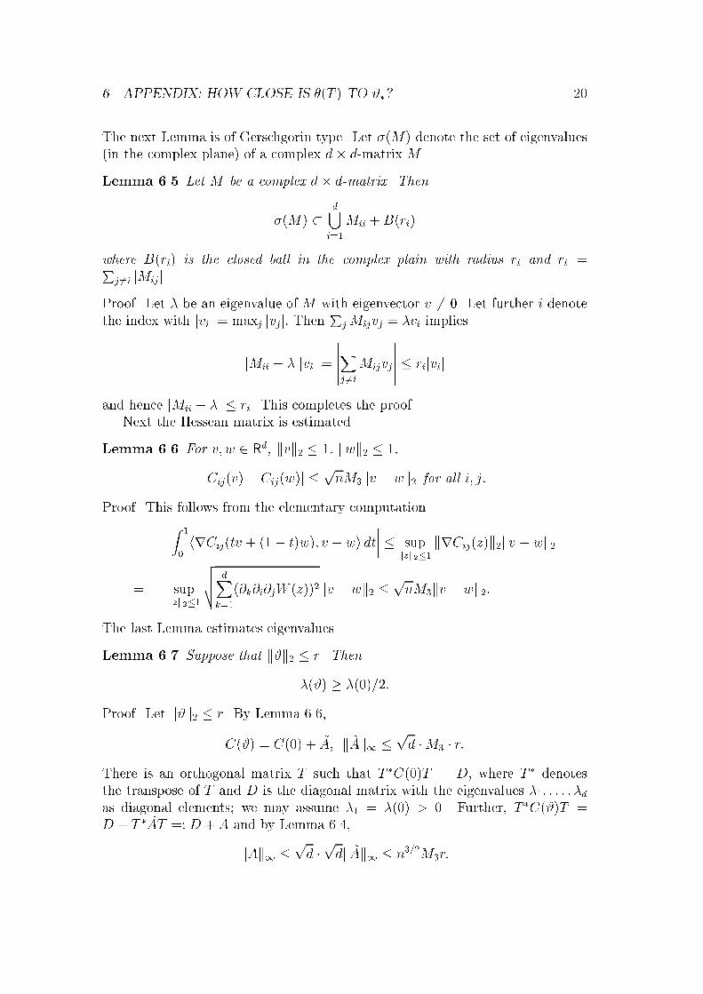
The next Lemma is of Gerschgorin type� Let �M denote the set of eigenvaluesin the complex plane of a complex d� d�matrix M �
Lemma �� Let M be a complex d� d�matrix Then
�M �d�i�
Mii �Bri
where Bri is the closed ball in the complex plain with radius ri and ri �Pj i jMijj
Proof� Let � be an eigenvalue of M with eigenvector v � �� Let further i denotethe index with jvij � maxj jvjj� Then PjMijvj � �vi implies
jMii � �jjvij �Xj i
Mijvj
� rijvij
and hence jMii � �j � ri� This completes the proof�Next the Hessean matrix is estimated�
Lemma � For v� w � Rd� kvk� � �� kwk� � ��
jCijv� Cijwj �pnMkv � wk� for all i� j�
Proof� This follows from the elementary computationZ �
�hrCijtv � �� tw� v � wi dt
� supkzk���
krCijzk�kv � wk�
� supkzk���
vuut dXk�
�k�i�jW z�kv � wk� �pnMkv � wk��
The last Lemma estimates eigenvalues�
Lemma �� Suppose that k�k� � r Then
�� � ����
Proof� Let k�k� � r� By Lemma ����
C� � C� � $A� k $Ak� �pd �M � r�
There is an orthogonal matrix T such that T �C�T � D� where T � denotesthe transpose of T and D is the diagonal matrix with the eigenvalues ��� � � � � �das diagonal elements� we may assume �� � �� � �� Further� T �C�T �D � T � $AT �� D � A and by Lemma ����
kAk� �pd �pdk $Ak� � n��Mr�

� APPENDIX� HOW CLOSE IS �T TO �� ��
Since �C� � �T �C�T � Lemma ��� gives
�� �n�i�
�i � Aii �Bri�
where ri �P
j i jAijj � d� �kAk�� By the de�nition of r�
�� � �� � jA�� � d� �kAk� � �� � dkAk�� ��� nkAk� � ��� d���Mr � ���
which had to be shown�Now the preparations for the proof of the Theorem are complete�Proof of Theorem ���� For kvk � r Lemma ��! yields the estimate
hv�rV vi ��v�Z �
�Ctv dt � v
��Z �
�hv� Ctvvi dt
�Z�tvkvk�� dt �
��
�kvk���
For the proof of �i� assume that k���k� � r� The set
I � fs � ���� � k�tk � r for all t � ���� s�g
is a closed interval� We are going to prove I � ����� If ��� � � then thesolution stays there and the assertion clearly holds� Otherwise �s � � for somes � ��� Let Ut � k�tk�� for t � ��� If s � I then
�Us � h�s� ��si � �h�s�rV �si� ���
�k�sk�� � ���Us � ��
Hence I is also open in ����� Since �� � I this implies I � ����� Theestimate for �U implies
Us � U�� exp���s� �� for s � ���
and hence
k�sk� � k��� exp����
�s� ��
� r exp
����
�s� ��
for s � ��
which proves �i��
� APPENDIX� HOW CLOSE IS �T TO �� ��
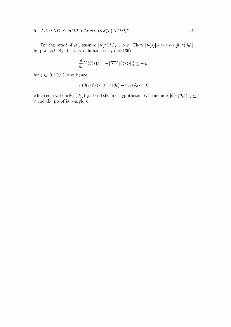
For the proof of �ii� assume k����k� � r� Then k�sk� � r on ��� ����by part �i�� By the very de�nition of �r and ���
d
dsV �s � �krV �sk�� � ��r
for s � ��� ���� and hence
V ���� � V ��� �r��� � �
which contradicts ���� � � and the �rst hypothesis� We conclude k����k� �r and the proof is complete�
REFERENCES ��
We thank B� Lani�Wayda� who pointed out to us the estimates in the Ap�pendix�
References
��� Benveniste A��M�etivier M� and Priouret P� ����� Adaptive Algo�rithms and Stochastic Approximations� Springer Verlag� Berlin HeidelbergNew York London Paris Tokyo HongKong Barcelona
��� Besag J� ��!�� Spatial Interaction and the Statistical Analysis of LatticeSystems with discussion� J of the Royal Statist Soc � B� � � ���%���
��� Besag J� ��!!� E�ciency of Pseudolikelihood for Simple Gaussian Field�Biometrika �� ���%���
��� Comets F� ����� On Consistency of a Class of Estimators for Exponen�tial Families of Markov random �elds on the Lattice� The Ann of Statist ��� ���%� �
��� Derevitzkii D�P� and Fradkov A�L� ��!�� Two Models for Analyzingthe Dynamics of Adaption Algorithms� Automation and Remote Control ���� ����!
��� Freidlin M�I� and Wentzell A�D� �� �� Random Perturbations ofDynamical Systems Springer Verlag� Berlin Heidelberg New York
�!� X� Guyon ����� Random Fields on a Network Springer Verlag� NewYork� Berlin
� � Guyon X� and K�unsch H�R� ����� Asymptotic Comparison of Esti�mators in the Ising Model� In� Stochastic Models� Statistical methods andAlgorithms in Image Analysis� P� Barone� A� Frigessi� M� Piccioni�eds� Lecture Notes in Statistics !�� Springer Verlag� �!!���
��� Jensen J�L� and K�unsch H�R� ����� On Asymptotic Normality ofPseudo Likelihood Estimates for Pairwise Interaction Processes� To appearin Ann Inst Statist Math
���� Ljung L� ��!!a� On Positive Real Transfer Functions and the Conver�gence of some Recursions� IEEE Trans on Automatic Control AC��� ���������
���� Ljung L� ��!!b� Analysis of Recursive Stochastic Algorithms� IEEETrans on Automatic Control AC��� �� �����!�
REFERENCES ��
���� Ljung L� ��! � Convergence of an Adaptive Filter Algorithm� Int J Control �� �� �!�����
���� M�etivier M� and Priouret P� �� !� Th&eor'emes de Conver�gence Presque Sure pour une Classe d�Algorithmes Stochastique 'a Pasd&Ecroissant� Probab Th Rel Fields ��� ���%��
���� Weizs�acker� H�v� andWinkler G� ����� Stochastic Integrals� Friedr�Vieweg ( Sohn� Braunschweig)Wiesbaden
���� Winkler G� ����� Image Analysis� Random Fields and Dynamic MonteCarlo Methods An Introduction to Mathematical Aspects Springer�Verlag�Berlin Heidelberg New York
���� Younes L� �� a� Estimation pour Champs de Gibbs et Application auTraitement d�Images� Universit&e Paris Sud Thesis
��!� Younes L� �� b� Estimation and Annealing for Gibbsian Fields� Ann Inst Henri Poincare ��� No� �� ���%���
�� � Younes L� �� �� Parametric Inference for Imperfectly Observed Gibb�sian Fields� Prob Th Rel Fields ��� ���%���