an adaptive optimization-based load shedding … adaptive optimization-based load shedding scheme in...

An Adaptive Optimization-Based Load Shedding Scheme in Microgrids

Amin Gholami, Tohid Shekari, and Xu Andy SunGeorgia Institute of Technology, Atlanta, Georgia 30332, USA

Email: [email protected], [email protected], [email protected]

Abstract

This paper proposes an adaptive optimization-basedapproach for under frequency load shedding (UFLS) inmicrogrids (µµµGs) following an unintentional islanding.In the first step, the total amount of load curtailmentsis determined based on the system frequency response(SFR) model. Then, the proposed mixed-integer linearprogramming (MILP) model is executed to find the bestlocation of load drops. The novel approach specifies theleast cost load shedding scenario while satisfying net-work operational limitations. A look-up table is arrangedaccording to the specified load shedding scenario to beimplemented in the network if the islanding event occursin the µµµG. To be adapted with system real-time conditions,the look-up table is updated periodically. The efficiency ofthe proposed framework is thoroughly evaluated in a testµµµG with a set of illustrative case studies.

Nomenclature

Indices, Sets, and Mappingsb Load block index.g Distributed generation (DG) index.i, j Bus indices.p Cosine linearization segment index.r Renewable energy source (RES) index.ΩBi

Set of load blocks at bus i.ΩL Set of lines.ΩG/ΩRES Set of DGs/RESs.ΩN Set of microgrid (µG) buses.ΩP Set of cosine linearization segments.MG/MRES Mapping of the set of DGs/RESs into

the set of buses.

ParametersBB Break point in cosine linearization seg-

ments.CB Cosine value in the associated break

point.H/D/R DG inertia/damping coeffi-

cient/governor droop.

G/B Conductance/susceptance of line.M,M ′ Sufficiently large positive numbers.pD/qD Pre-fault active/reactive power con-

sumption of load obtained from stateestimation (SE).

pRES/qRES Pre-fault active/reactive power produc-tion of RES obtained from SE.

pG,0 Active power generation of DG beforethe load shedding.

PM µG pre-fault energy exchange with theupstream grid obtained from SE.

PMthr The minimum amount of PM whichactivates the load shedding process.

PMthr,SSF/DF Steady-state/dynamic threshold of PM .pShed Minimum total amount of load drops.pShedSSF /p

ShedDF Total amount of load shedding sat-

isfying steady-state/dynamic frequencylimitation.

RU/RD Ramp-up/down limit of DG.S Capacity (apparent power) of DG.tShed/tmin Instants when the load shedding is im-

plemented and minimum dynamic fre-quency occurs.

V ∗ Pre-fault bus voltage magnitude ob-tained from SE.

τT /τV Turbine/governor valve time constantof DG.

λV OLL Value of lost loads (VOLL).κPI/κPC/κPP

Coefficient of constantimpedance/constant current/constantpower term in active power load.

κQI/κQC/κQP

Coefficient of constantimpedance/constant current/constantpower term in reactive power load.

∆fSSF /∆fDF

Steady-state/nadir value of frequencydeviation.

α1, α2, α3,β1, β2, β3, $,m1,m2,m3,c1, c2, c3, φ,δ1, δ2, δ3, δ4

Axillary continuous parameters.

Proceedings of the 51st Hawaii International Conference on System Sciences | 2018

URI: http://hdl.handle.net/10125/50225ISBN: 978-0-9981331-1-9(CC BY-NC-ND 4.0)

Page 2660

VariablesfP /fQ Active/reactive power flow of line.I Current flow of line.pG/qG Active/reactive power output of DG

following the load shedding process.pD/qD Active/reactive power consumption of

load following the load shedding pro-cess.

V Voltage magnitude of bus following theload shedding process.

x Binary variable indicating the loadshedding status of load (0/1).

αP /αQ Axillary continuous variable.ω Piecewise linear approximation of

cos (θi − θj).s/v Positive/binary variable used in cosine

linearization.

Symbols and Functionsu (•) Unit step function.(•)min /max Symbol for variable lower/upper limit.

1. Introduction

In recent years, the proliferation of distributed energyresources (DERs) has led to an increase in on-site elec-tricity service procurement for customers. This new trendhas a set of advantages and disadvantages over the con-ventional centralized power generation paradigm in termsof reliability, cost of maintenance, economies of scale,resiliency, and sustainability, to name a few [1]. Moreover,deploying DERs in a widespread and efficient mannerrequires practical mechanisms to identify and resolve thechallenges of integration. In this context, microgrids (µGs)are emerging as a flexible way to aggregate DERs. TheDepartment of Energy (DOE) defines a µG as “a groupof interconnected loads and DERs within clearly definedelectrical boundaries that acts as a single controllableentity with respect to the grid. A µG can connect anddisconnect from the grid to enable it to operate in bothgrid-connected or island mode” [2].

An unintentional islanding usually occurs in µGs inthe event of unforeseen faults in the upstream grid. IEEE929-1988 Std. [3] necessitates the disconnection of DERsonce the unintentional islanding event happens in the µG.Furthermore, IEEE 1547-2003 Std. [4] enforces DERs todetect the unintentional islanding and cease energizing theµG within maximum 2 sec. following the islanding event.Therefore, in the case of unintentional islanding, blackoutsseem inevitable.

It goes without saying that the current practice ofdisconnecting the DERs following an islanding event is

not economical since it imposes immense costs on the µG.When a µG with DERs is islanded, usually the frequencywill change. The frequency will either go up if there isexcess generation or down if there is excess load. Theformer can be controlled by reducing the output powerof the distributed generators (DGs) or other DERs [5].However, coping with the latter is more challenging. It isworth mentioning that in the normal operating condition,photovoltaic (PV) systems usually use maximum powerpoint tracking and variable speed wind turbines optimizepower coefficient (Cp) to produce maximum power. Thus,if all of the DGs are operating at maximum power andthe frequency still goes down, some loads have to beshed to bring the frequency back to the allowable range.Nonetheless, it is possible that PV generators and windturbines withhold production (these resources are non-dispatchable, but curtailable), and this is a growing trend inpower system operation which provides further flexibility.

To address the weaknesses of conventional under fre-quency load shedding (UFLS) scheme, researchers haveproposed adaptive load shedding schemes, which can beclassified into two main categories: decentralized andcentralized algorithms. Decentralized approaches use localvoltage and frequency signals at each bus to make thedecision about the load shedding process at that bus.Indeed, using these algorithms, the location, speed, andthe amount of load curtailments are adjusted adaptively topreserve the system stability following severe incidents.

Centralized methods, on the other hand, use the datagathered from the grid in order to decide which load tobe shed. The centralized schemes proposed in [6] droploads at different buses based on their VQ margin andpost-fault voltage magnitude. Reference [7] adopts bothvoltage and frequency information provided by phasormeasurement units (PMUs) to implement the appropriateload shedding scenario in the network. Other centralizedmethods determine the amount and location of load dropsaccording to the complete post-fault information about thenetwork [8]–[11].

Owing to the differences between µGs and bulk powersystems, the load shedding mechanism for a µG shouldbe treated differently. µGs usually have small generatorsand, hence, small inertia. As a consequence, the frequencydeclines more rapidly in µGs. This paper presents a cen-tralized adaptive optimization-based load shedding schemeto curtail the minimum amount of loads to preserve the µGstability following an unintentional islanding event. Thedeveloped technique arranges a look-up table includingthe optimum amount and location of load curtailments.The main contributions of the new methodology can besummarized as follows:

1) Given a specific amount of power exchange betweenthe µG and the upstream grid, the optimal total

661

amount of load shedding is determined. Specifically,this value depends on the response of both thegenerators and the loads to the islanding event.These responses are reflected in the system fre-quency response (SFR) model as well as the µGdynamic and static frequency limitations.

2) We developed a mixed-integer linear programming(MILP) model for obtaining the amount of loaddrops at different buses. In the optimization model,an approximation of the µG AC operational limita-tions are considered to ensure the network securityfollowing the islanding event.

3) A hierarchical structure is proposed in this paperso as to reduce both data and communication re-quirements of the new centralized algorithm. Togive more explanation, the majority of the neededinformation are periodically updated and only apractically tractable share is gathered in real time.

The rest of this paper is organized as follows. Section2 presents the overview of the proposed load sheddingalgorithm. In Section 3, a method for estimating thetotal amount of load curtailments is developed. Section4 is devoted to introducing the optimization-based loadshedding scheme. Section 5 exhibits the efficiency of thenovel approach using an illustrative case study. Eventually,conclusion is given in Section 6.

2. Overview of the Proposed Load SheddingAlgorithm

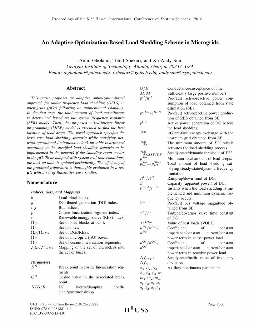
The general framework of the proposed load sheddingalgorithm is depicted in Fig. 1. In the first step, theµG master controller (µGMC) gathers the network dataperiodically (e.g., ∆T = 5 min.) and runs the stateestimation (SE) in order to obtain the proposed scheme’sinput parameters (operating point of the µG, load andgeneration data, and µG topology). Then, the optimumtotal amount of load curtailments is determined basedon the µG SFR model and the power exchange betweenthe µG and the upstream grid. Note that the obtainedtotal amount of load drops satisfies the µG dynamic andstatic frequency limitations. The total amount of loadshedding along with the SE data are fed into the proposedoptimization model in order to arrange a look-up tableincluding the location of load drops as well as appropriatepost load shedding strategies. On the other side, thestatus of point of common coupling (PCC) circuit breakeris monitored using indication (i.e., binary) data. If anunintentional islanding happens and the amount of powermismatch is greater than a specific value, the pre-specifiedload shedding scenarios will be implemented in the µG.Detailed explanations about different parts of the proposedmethodology are provided in the following sections.

Real-Time Analysis

Monitor the Circuit Breaker in PCC

Yes

Offline Analysis

Perform Data Polling and State Estimation Periodically

Determine the Total Amount of Load Curtailments

Run the Proposed MILP Model

Look-Up TableImplement the Look-Up Table in the Microgrid

Unintentional Islanding Event Occurs?

No

Load SheddingLoad Shedding Is

Required?

Yes

No

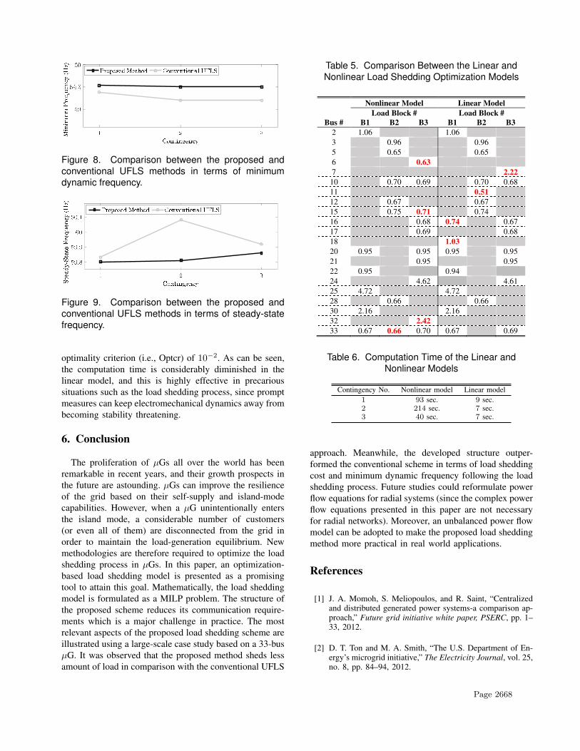
Figure 1. The general framework of the proposed loadshedding algorithm.

Time

Frequency

Steady-State Frequency

Minimum Dynamic Frequency

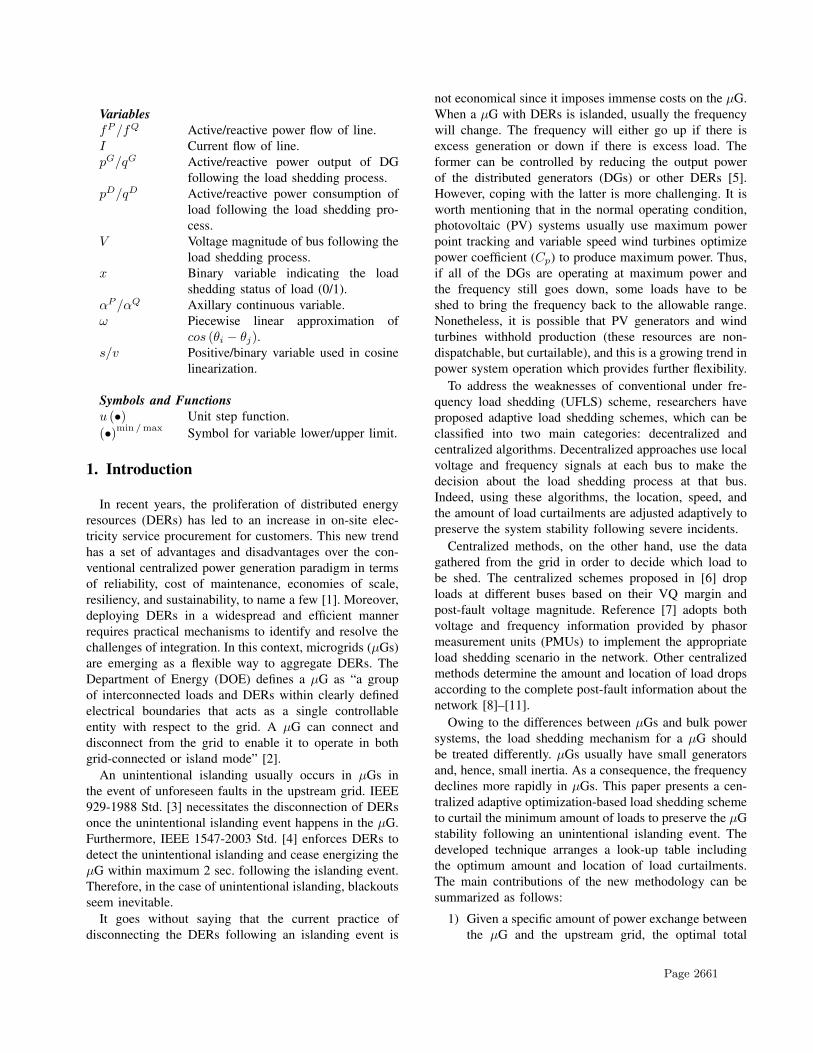
Figure 2. A typical frequency response of a µGfollowing an unintentional islanding event.

3. Optimal Amount and Threshold for Acti-vation of Load Shedding

The aim of this section is to determine the minimumamount of load curtailments as well as a threshold foractivation of the load shedding process, while the µGdynamic and steady-state frequency limitations are satis-fied. The minimum dynamic and steady-state frequenciesare indicated in a typical frequency response of a µGfollowing an unintentional islanding event, Fig. 2.

3.1. Frequency Response of the µG to an Island-ing Event

As the first step, the frequency response of the µG toan islanding event should be specified. To do so, we usethe aggregated SFR model of the µG as shown in Fig.3 [12], [13]. This model is an equivalent single machine

Page 2662

12Hs+D

1τV s+1

1τT s+1

1R

∆P ∆f

−

Figure 3. Block diagram of the adopted SFR model.

model of all DGs in the µG, where the frequency of thecenter of inertia is considered by ignoring intermachineoscillations. The transfer function 1

2Hs+D in the forwardpath represents the swing equation of the equivalent DGas well as the effects of the µG loads which are lumpedinto a single damping constant D. Moreover, the transferfunctions in the feedback loop are associated with thegovernor droop, governor time constant, and turbine timeconstant of the equivalent DG [13].

The transfer function of the adopted SFR model can bewritten as (1).

H (s) =α1s

2 + α2s+ α3

s3 + β1s2 + β2s+ β3, (1)

where

α1 =1

2H,α2 =

1

2H

(1

τT+

1

τV

), α3 =

1

2HτT τV

β1 =D

2H+

1

τT+

1

τV, β2=

1

τT τV+

D

2H

(1

τT+

1

τV

)β3 =

1R +D

2HτT τV.

3.2. Threshold for Activation of Load SheddingScheme

In the wake of an unintentional islanding, the gover-nors and loads in the µG will respond to the incident,thereby compensating for a portion of power mismatch.Consequently, load shedding is not necessary in all cases.Specifically, the minimum amount of power mismatchwhich would activate the load shedding process is obtainedby (2).

PMthr = minPMthr,SSF , P

Mthr,DF

, (2)

where PMthr,SSF and PMthr,DF are the steady-state anddynamic thresholds of PM , respectively. Suppose that theµG is not equipped with any load shedding scheme. In thiscondition, if an unintentional islanding happens, the inputpower deviation of the SFR model in Fig. 3 is defined as(3).

∆P (t) = −PMu (t) ,∆P (s) =−PM

s. (3)

Hence, the Laplace form of the frequency deviation func-tion is obtained as (4).

∆f (s) = H (s) ∆P (s) =

F(s)︷︸︸︷α1s

2 + α2s+ α3

s (s3 + β1s2 + β2s+ β3)

(−PM

).

(4)

Accordingly, F (s) can be decomposed into three termsusing partial-fraction decomposition as follows:

F (s) =α1s

2 + α2s+ α3

s (s3 + β1s2 + β2s+ β3)

=δ1s

+δ2

s−m1+

δ3s+ δ4s2 +m2s+m3

,

(5)

where

m2 =2

3

(β1 −

c12− c2

2c1

),

m3 =1

9

[(β1 −

c12− c2

2c1

)2

+3

4

(c1 −

c2c1

)2],

c1 =3

√c3 +

√c23 − 4c322

,m1 =−1

3

(β1 + c1 +

c2c1

),

c2 = β21 − 3β2, c3 = 2β3

1 − 9β1β2 + 27β3,

δ1 =α3

β3, δ2 =

α1m21 + α2m1 + α3

m31 +m2m2

1 +m3m1,

δ3 = − (δ1 + δ2) , δ4 = (δ1β2 + δ2m3 − α2) /m1.

Taking the inverse Laplace transform of F (s), F (t) isgiven by:

F (t) =

(δ1 + δ2e

m1t +δ3e

−m22 t

cos (φ)cos ($t+ φ)

)u (t) ,

(6)where

$ =

√m3 −

m22

4, cosφ =

$√$2 +

(m2

2 −δ3δ4

)2.

Therefore, ∆f (t) can be written as (7).

∆f (t) = −PMF (t) . (7)

3.2.1. Steady-State Threshold of PM . Given ∆f (t) as(7), ∆fSSF (i.e., steady state frequency deviation) can becomputed as (8).

∆fSSF = limt→∞

∆f (t) =(−PM

)δ1. (8)

The load shedding process will be triggered if the valueof ∆fSSF exceeds a given threshold ∆fmax

SSF , that is:∣∣(−PM) δ1∣∣ ≥ |∆fmaxSSF | . (9)

Page 2663

Therefore, the minimum amount of PM which violatesthe steady-state frequency limitation, and thus, triggers theload shedding process is acquired as follows:

PM ≥ |∆fmaxSSF |

(D +

1

R

). (10)

Accordingly, we define the right hand side of (10) asthe steady state threshold of PM .

3.2.2. Dynamic Threshold of PM . The time when thefrequency nadir happens (i.e., when the lowest frequencyis reached before the frequency starts to recover) can becalculated by putting the first derivative of ∆f (t) equalto zero:

tmin = min

t : t > 0,

d∆f (t)

dt= 0

. (11)

Accordingly, the second trigger for the load sheddingprocess is associated with the violation of nadir frequencylimitation, that is:

|∆f (tmin)| ≥ |∆fmaxDF | . (12)

The solution to this inequality in terms of PM , willprovide another criterion or lower bound (denoted byPMthr,DF in (2)) for the activation of the load sheddingprocess.

3.3. Optimal Amount of Load Shedding

The minimum total amount of load curtailments satis-fying both steady-state and dynamic frequency limitationsis calculated as (13).

pShed = maxpShedSSF , p

ShedDF

, (13)

where pShedSSF and pShedDF are obtained as follows. Supposethat the load shedding scheme is implemented in the µGwith a delay of tShed, subsequent to the unintentionalislanding event. Accordingly, the input power deviationof the SFR model will be defined as (14).

∆P (t) = −PMu (t) + pShedu(t− tShed

). (14)

Taking the Laplace transform of ∆P (t) yields

∆P (s) =1

s

(−PM + pShede−t

Sheds). (15)

Hence, the Laplace form of the frequency deviationfunction is obtained as (16).

∆f (s) = F(s)(−PM + pShede−t

Sheds), (16)

where, F (s) is obtained from (5). Taking the inverseLaplace transform of (16), ∆f (t) can be written as (17)below

∆f (t) = −PMF (t) + pShedF(t− tShed

), (17)

where F (t) is calculated in (6).

3.3.1. Load Shedding Value Based on the Steady-StateFrequency Limitation. Given ∆f (t) as (17), ∆fSSF canbe computed as (18) [8].

∆fSSF = limt→∞

∆f (t) =(−PM + pShedSSF

)δ1. (18)

Therefore, the minimum total amount of load shed-ding satisfying the steady-state frequency limitation (i.e.,|∆fSSF | ≤ |∆fmax

SSF |) is acquired as follows:

pShedSSF = PM − |∆fmaxSSF |

(D +

1

R

). (19)

3.3.2. Load Shedding Value Based on the DynamicFrequency Limitation. Similar to Section 3.2.2, the timewhen the frequency nadir happens is acquired by solving(11), where ∆f (t) is calculated according to (17). Byapplying the nadir frequency limitation (i.e., |∆fDF | ≤|∆fmax

DF |), the minimum amount of load shedding satisfy-ing dynamic frequency limitation (i.e., pShedDF ) is obtained.It should be noted that the proposed method in this paperis aimed at bringing the frequency to the permissible range(according to ∆fmax

SSF and ∆fmaxDF ) with the minimum

amount of load shedding. Obviously, the frequency shouldfinally bring back to 60 Hz, but this transition can happenwith a short delay (2-3 minutes) with the advantage ofshedding fewer loads. Subsequent to load shedding, DERswill try to bring the frequency back to 60 Hz. If thiscannot happen (e.g., due to some limitations in the outputof DERs), further loads will be curtailed. This idea isconsistent with the load-frequency control mechanismswhich are done in three different successive steps (i.e.,primary control, secondary control, tertiary control).

4. Optimization-Based Load SheddingScheme

4.1. Basic Model

In this section, the basic model of the µG load sheddingscheme is presented. The objective function and problemconstraints are outlined as follows:

min∑i∈ΩN

∑b∈ΩBi

λV OLLib (1− xib) pDib (20)

subject to∑g:(g,i)∈MG

pGg +∑

r:(r,i)∈MRES

pRESr −∑b∈ΩBi

xibpDib =

∑(i,j)∈ΩL

fP(i,j),∀i ∈ ΩN

(21)

Page 2664

∑g:(g,i)∈MG

qGg +∑

r:(r,i)∈MRES

qRESr −∑b∈ΩBi

xibqDib =

∑(i,j)∈ΩL

fQ(i,j),∀i ∈ ΩN

(22)

fP(i,j) = G(i,j)

(V 2i − ViVjcos (θi − θj)

)−B(i,j)

(ViVjsin (θi − θj)

),∀ (i, j) ∈ ΩL

(23)

fQ(i,j) = −B(i,j)

(V 2i − ViVjcos (θi − θj)

)−G(i,j)

(ViVjsin (θi − θj)

),∀ (i, j) ∈ ΩL

(24)

−fP,max(i,j) ≤ fP(i,j) ≤ f

P,max(i,j) ,∀ (i, j) ∈ ΩL (25)

−fQ,max(i,j) ≤ fQ(i,j) ≤ f

Q,max(i,j) ,∀ (i, j) ∈ ΩL (26)

fP(i,j) + fP(j,i) =G(i,j)

G2(i,j) +B2

(i,j)

∣∣I(i,j)∣∣2 ≤ fP,Loss,max(i,j)

=G(i,j)

G2(i,j) +B2

(i,j)

∣∣∣Imax(i,j)

∣∣∣2,∀ (i, j) ∈ ΩL

(27)

V mini ≤ Vi ≤ V max

i ,∀i ∈ ΩN (28)

pDib = pDib

(κPIib (Vi/V

∗i )

2

+ κPCib (Vi/V∗i ) + κPPib

),∀i ∈ ΩN , b ∈ ΩBi

(29)

qDib = qDib

(κQIib (Vi/V

∗i )

2

+ κQCib (Vi/V∗i ) + κQPib

),∀i ∈ ΩN , b ∈ ΩBi

(30)

−RDg ≤ pGg − pG,0g ≤ RUg ,∀g ∈ ΩG (31)

pG,ming ≤ pGg ≤ pG,max

g ,∀g ∈ ΩG (32)

qG,ming ≤ qGg ≤ qG,max

g ,∀g ∈ ΩG (33)

∑i∈ΩN

∑b∈ΩBi

(1− xib)pDib ≥ pShed (34)

xib ∈ 0, 1 ,∀i ∈ ΩN , b ∈ ΩBi. (35)

The objective function, (20), is the load shedding costin the µG, which should be minimized. λV OLLib is a

socioeconomic parameter and varies for different types ofloads (e.g., industrial, commercial, agricultural, residential,and general loads). The group of equations (21)–(24) isrelated to the AC power flow equations. Line flow limitsand bus voltage constraints are modeled through (25)–(27) and (28), respectively. Incorporation of a suitableload model for µG loads plays an important role in powersystem stability studies [9]. Therefore, the active and re-active power demands at different buses are modeled withvoltage-dependent load model referred to as ZIP model,(29)–(30) [14]. Constraints (31)–(33) revolve around DG’sramp-up and ramp-down limits (31) and active and reactivepower generation limits of DGs (32)–(33). The minimumtotal load shedding constraint is expressed as (34), andfinally, the status of loads is characterized by a binaryvariable in (35).

4.2. Linearization of the Basic Model

The developed problem in Section 4.1 is a mixed-integernonlinear programming (MINLP) model. In order to attaincomputational efficiency, the nonlinear equations ought tobe linearized. The nonlinear terms xibpDib and xibq

Dib in

(21)–(22) and (34) are the product of a binary and continu-ous variables. We can linearize these terms with the big-Mmethod by introducing auxiliary semi-continuous variables(i.e., αPib

∆= xibp

Dib and αQib

∆= xibq

Dib ) and the set of

equations (36)–(39). In order to reduce the integrality gapin the linearized version of the aforementioned constraints,Big-Ms (i.e., Mib and M ′ib) should be as small as possible,and it is usually challenging to determine correct valuesfor them to use for each specific implementation. However,in this particular application, we can set Mib = pDib andM ′ib = qDib , ∀i ∈ ΩN , b ∈ ΩBi

. Note that these data (i.e.,the upper bounds of active and reactive loads) are usuallyavailable in any system.

Moreover, considering reasonable assumptions given inTable 1 [15], AC power flow equations are replaced bytheir piecewise linear approximation form as (40)–(49).Finally, considering the permissible range for bus voltagemagnitudes at different buses (i.e., 0.9 ≤ Vi, V

∗i ≤ 1.1),

(29)–(30) can be reasonably approximated by (50)–(51)[9]. With these changes, the proposed model is trans-formed into an MILP model.

− (1− xib)Mib ≤ αPib − pDib≤Mib (1− xib) ,∀i ∈ ΩN , b ∈ ΩBi

(36)

−xibMib ≤ αPib ≤Mibxib,∀i ∈ ΩN , b ∈ ΩBi(37)

Page 2665

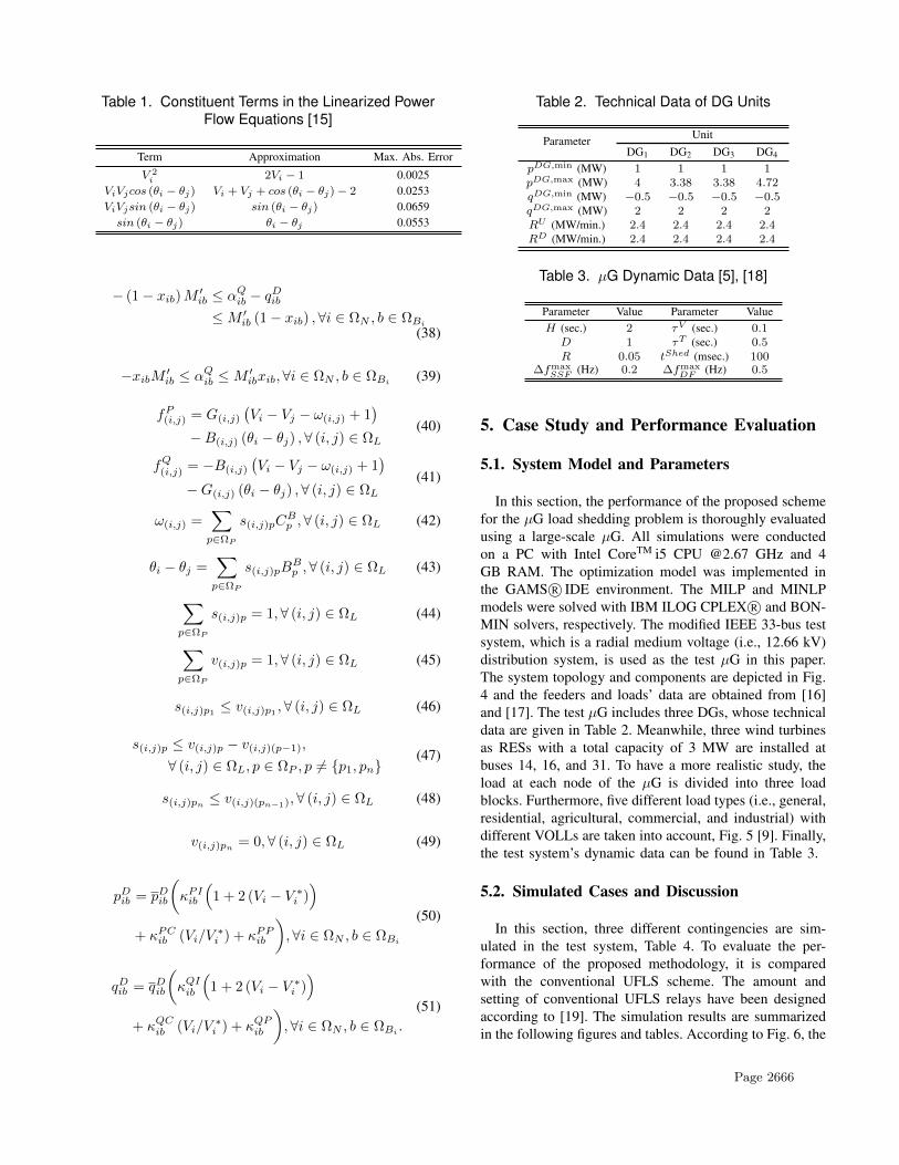
Table 1. Constituent Terms in the Linearized PowerFlow Equations [15]

Term Approximation Max. Abs. Error

V 2i 2Vi − 1 0.0025

ViVjcos (θi − θj) Vi + Vj + cos (θi − θj) − 2 0.0253ViVjsin (θi − θj) sin (θi − θj) 0.0659sin (θi − θj) θi − θj 0.0553

− (1− xib)M ′ib ≤ αQib − q

Dib

≤M ′ib (1− xib) ,∀i ∈ ΩN , b ∈ ΩBi

(38)

−xibM ′ib ≤ αQib ≤M

′ibxib,∀i ∈ ΩN , b ∈ ΩBi (39)

fP(i,j) = G(i,j)

(Vi − Vj − ω(i,j) + 1

)−B(i,j) (θi − θj) ,∀ (i, j) ∈ ΩL

(40)

fQ(i,j) = −B(i,j)

(Vi − Vj − ω(i,j) + 1

)−G(i,j) (θi − θj) ,∀ (i, j) ∈ ΩL

(41)

ω(i,j) =∑p∈ΩP

s(i,j)pCBp ,∀ (i, j) ∈ ΩL (42)

θi − θj =∑p∈ΩP

s(i,j)pBBp ,∀ (i, j) ∈ ΩL (43)

∑p∈ΩP

s(i,j)p = 1,∀ (i, j) ∈ ΩL (44)

∑p∈ΩP

v(i,j)p = 1,∀ (i, j) ∈ ΩL (45)

s(i,j)p1 ≤ v(i,j)p1 ,∀ (i, j) ∈ ΩL (46)

s(i,j)p ≤ v(i,j)p − v(i,j)(p−1),

∀ (i, j) ∈ ΩL, p ∈ ΩP , p 6= p1, pn(47)

s(i,j)pn ≤ v(i,j)(pn−1),∀ (i, j) ∈ ΩL (48)

v(i,j)pn = 0,∀ (i, j) ∈ ΩL (49)

pDib = pDib

(κPIib

(1 + 2 (Vi − V ∗i )

)+ κPCib (Vi/V

∗i ) + κPPib

),∀i ∈ ΩN , b ∈ ΩBi

(50)

qDib = qDib

(κQIib

(1 + 2 (Vi − V ∗i )

)+ κQCib (Vi/V

∗i ) + κQPib

),∀i ∈ ΩN , b ∈ ΩBi .

(51)

Table 2. Technical Data of DG Units

Parameter UnitDG1 DG2 DG3 DG4

pDG,min (MW) 1 1 1 1pDG,max (MW) 4 3.38 3.38 4.72qDG,min (MW) −0.5 −0.5 −0.5 −0.5qDG,max (MW) 2 2 2 2RU (MW/min.) 2.4 2.4 2.4 2.4RD (MW/min.) 2.4 2.4 2.4 2.4

Table 3. µG Dynamic Data [5], [18]

Parameter Value Parameter ValueH (sec.) 2 τV (sec.) 0.1D 1 τT (sec.) 0.5R 0.05 tShed (msec.) 100

∆fmaxSSF (Hz) 0.2 ∆fmax

DF (Hz) 0.5

5. Case Study and Performance Evaluation

5.1. System Model and Parameters

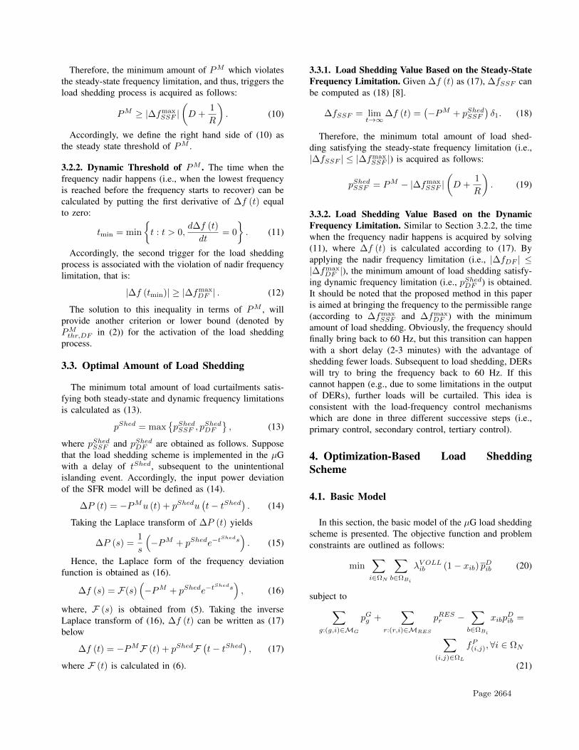
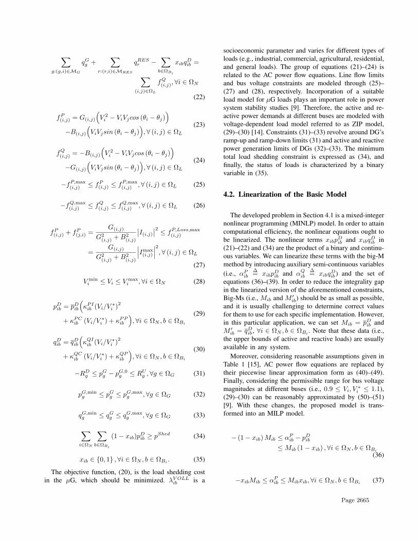
In this section, the performance of the proposed schemefor the µG load shedding problem is thoroughly evaluatedusing a large-scale µG. All simulations were conductedon a PC with Intel CoreTM i5 CPU @2.67 GHz and 4GB RAM. The optimization model was implemented inthe GAMS R© IDE environment. The MILP and MINLPmodels were solved with IBM ILOG CPLEX R© and BON-MIN solvers, respectively. The modified IEEE 33-bus testsystem, which is a radial medium voltage (i.e., 12.66 kV)distribution system, is used as the test µG in this paper.The system topology and components are depicted in Fig.4 and the feeders and loads’ data are obtained from [16]and [17]. The test µG includes three DGs, whose technicaldata are given in Table 2. Meanwhile, three wind turbinesas RESs with a total capacity of 3 MW are installed atbuses 14, 16, and 31. To have a more realistic study, theload at each node of the µG is divided into three loadblocks. Furthermore, five different load types (i.e., general,residential, agricultural, commercial, and industrial) withdifferent VOLLs are taken into account, Fig. 5 [9]. Finally,the test system’s dynamic data can be found in Table 3.

5.2. Simulated Cases and Discussion

In this section, three different contingencies are sim-ulated in the test system, Table 4. To evaluate the per-formance of the proposed methodology, it is comparedwith the conventional UFLS scheme. The amount andsetting of conventional UFLS relays have been designedaccording to [19]. The simulation results are summarizedin the following figures and tables. According to Fig. 6, the

Page 2666

1

Abstract—

I. CASE STUDY AND PERFORMANCE EVALUATION

In this section, the performance of the proposed scheme for

the µG load shedding problem is thoroughly evaluated using a

large-scale µG. All simulations were conducted on a PC with

Intel CoreTM i7 CPU @3.20 GHz and 4 GB RAM. The MILP

optimization model was implemented in the GAMS®IDE

environment [**] and the model was solved with IBM ILOG

CPLEX ® 12.4 solver [***].

The modified IEEE 33-bus test system is a medium voltage

(i.e., 12.66 kV) distribution network which is used as the test

µG in this paper. The µG topology and components are

depicted in Fig. 4 and the feeders’ data are obtained from

[***]. Note that the switchable lines are also depicted in this

figure by red dashed trajectories. The location and size of DGs

are determined according to [***]. The technical

characteristics of the DGs can be found in Tables II.

Three RESs with a total capacity of 3 MW are installed at

buses 14, 16, and 31. As µG buses are located in a small

geographical region, the outputs of the three RESs are

considered to be the same in our study.

Fig. 4. Single line diagram of the simulated µG.

Adoption of a reasonable model for representing the load

behavior plays a prominent role in both voltage and frequency

stability analyses. To have a more realistic study, the load at

each node of the µG is divided into three load blocks.

Moreover, five different load types (including general,

residential, agricultural, commercial, and industrial) are taken

into account. The contribution percentage as well as the VOLL

of these loads are provided in Table III.

TABLE II TECHNICAL CHARACTERISTICS OF DEPLOYED CONVENTIONAL DGS

Unit Technical Constraints

(MW)G

iP

(MW)G

iP (MVAr)G

iQ

(MW)G

iQ R H

DG1 3 0.21 2.1 -2.1 2 2

DG2 2 0.19 1.9 -1.9 2 2

DG3 2 0.19 1.9 -1.9 2 2

DG4 3 0.22 2.2 -2.2 2 2

TABLE I VOLL FOR VARIOUS LOAD TYPES [22]

Load Type VOLL ($/MW) Contribution Percentage (%)

General 650 16.4

Residential 190 6

Agricultural 420 23.5

Commercial 4365 11.6

Industrial 5172 42.5

A. Results and Discussion

Considering a mip gap of 0%, the computation time was 20

seconds which further illustrates the practical merits of the

proposed framework in case of real-scale networks.

Simulation and results

Amin Gholami, Student Member, IEEE, Tohid Shekari, Student Member, IEEE, Farrokh Aminifar, Senior Member, IEEE, and Mohammad Shahidehpour, Fellow, IEEE

Upstream

Network MG Operator

1 2 3 7 6 5 4 8 9 10 11

19 18 17 16 15

14 13 12

20 21 22

33 32 31 30 29 28 27 26

23 24 25

PCC

Substation

DG4

RES1

RES3

DG3 RES2

DG1

DG2

Figure 4. Single line diagram of the simulated µG [17].

3

General Residential Agricultural Commercial Industrial0

1000

2000

3000

4000

5000

6000

VOLL

($/M

W)

General Residential Agricultural Commercial Industrial0

1000

2000

3000

4000

5000

6000

VOLL

($/M

W)

Figure 5. VOLL for different types of loads.

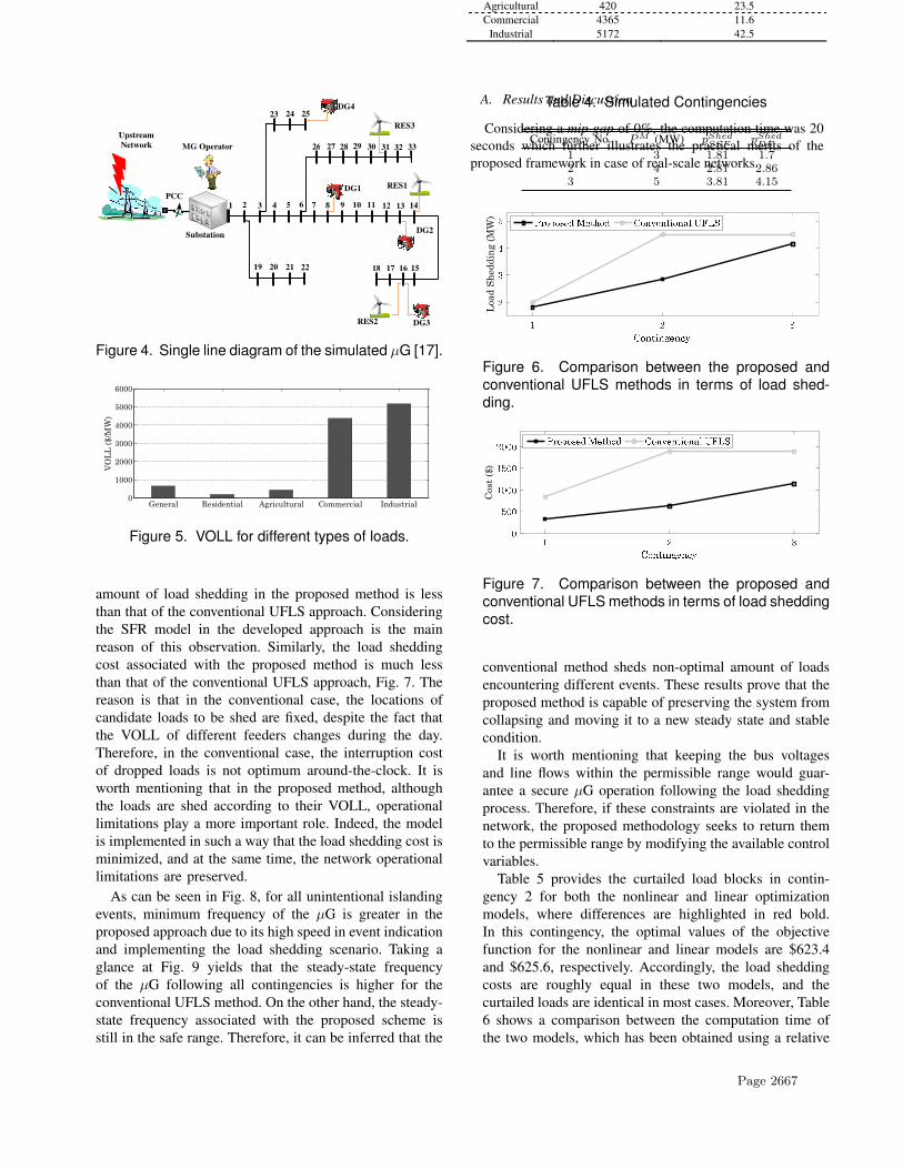
amount of load shedding in the proposed method is lessthan that of the conventional UFLS approach. Consideringthe SFR model in the developed approach is the mainreason of this observation. Similarly, the load sheddingcost associated with the proposed method is much lessthan that of the conventional UFLS approach, Fig. 7. Thereason is that in the conventional case, the locations ofcandidate loads to be shed are fixed, despite the fact thatthe VOLL of different feeders changes during the day.Therefore, in the conventional case, the interruption costof dropped loads is not optimum around-the-clock. It isworth mentioning that in the proposed method, althoughthe loads are shed according to their VOLL, operationallimitations play a more important role. Indeed, the modelis implemented in such a way that the load shedding cost isminimized, and at the same time, the network operationallimitations are preserved.

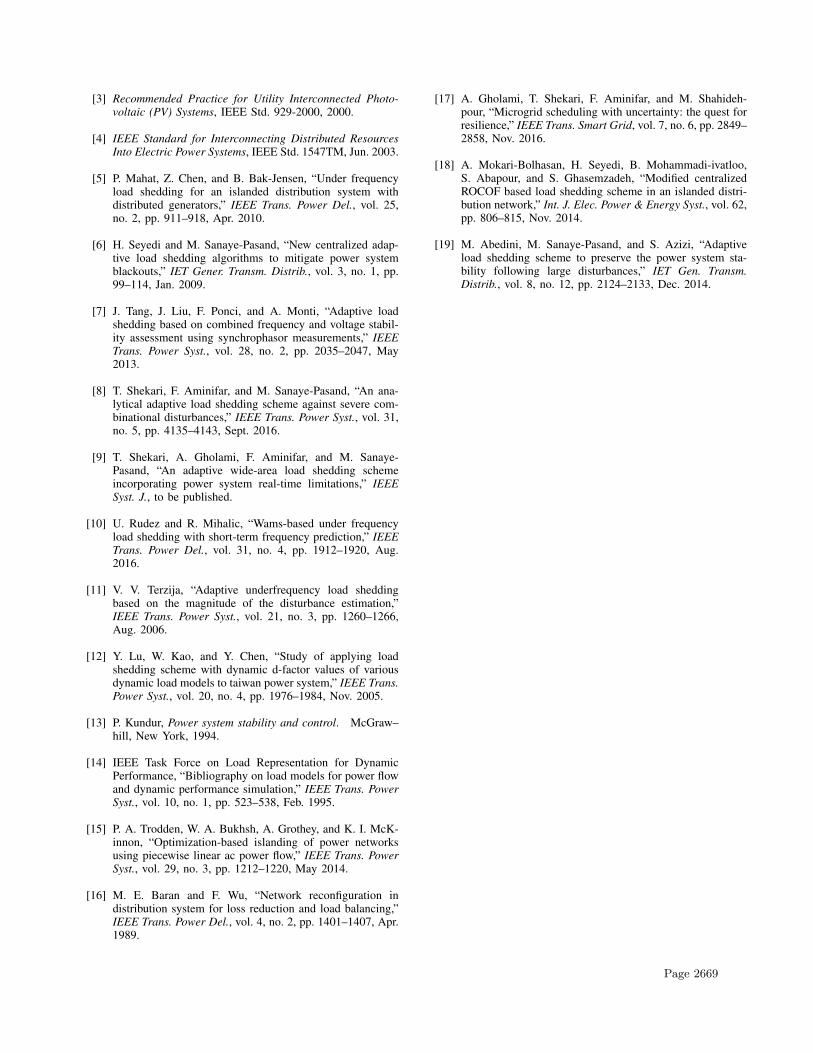
As can be seen in Fig. 8, for all unintentional islandingevents, minimum frequency of the µG is greater in theproposed approach due to its high speed in event indicationand implementing the load shedding scenario. Taking aglance at Fig. 9 yields that the steady-state frequencyof the µG following all contingencies is higher for theconventional UFLS method. On the other hand, the steady-state frequency associated with the proposed scheme isstill in the safe range. Therefore, it can be inferred that the

Table 4. Simulated Contingencies

Contingency No. PM (MW) pShedSSF pShed

DF

1 3 1.81 1.72 4 2.81 2.863 5 3.81 4.15

1

Abstract—

In this section,

Load Shedding (MW)

Cost ($)

the performance of the proposed scheme for the µG load

shedding problem is thoroughly evaluated using a large-scale

µG. All simulations were conducted on a PC with Intel

CoreTM i7 CPU @3.20 GHz and 4 GB RAM. The MILP






















NES imulation and results


Upstream

Network MG Operator

1 2 3 7 6 5 4 8 9 10 11

19 18 17 16 15

14 13 12

20 21 22

33 32 31 30 29 28 27 26

23 24 25

PCC

Substation

DG4

RES1

RES3

DG3 RES2

DG1

DG2

Figure 6. Comparison between the proposed andconventional UFLS methods in terms of load shed-ding.

1

Abstract—

In this section,

Load Shedding (MW)

Cost ($)




























Upstream

Network MG Operator

1 2 3 7 6 5 4 8 9 10 11

19 18 17 16 15

14 13 12

20 21 22

33 32 31 30 29 28 27 26

23 24 25

PCC

Substation

DG4

RES1

RES3

DG3 RES2

DG1

DG2

Figure 7. Comparison between the proposed andconventional UFLS methods in terms of load sheddingcost.

conventional method sheds non-optimal amount of loadsencountering different events. These results prove that theproposed method is capable of preserving the system fromcollapsing and moving it to a new steady state and stablecondition.

It is worth mentioning that keeping the bus voltagesand line flows within the permissible range would guar-antee a secure µG operation following the load sheddingprocess. Therefore, if these constraints are violated in thenetwork, the proposed methodology seeks to return themto the permissible range by modifying the available controlvariables.

Table 5 provides the curtailed load blocks in contin-gency 2 for both the nonlinear and linear optimizationmodels, where differences are highlighted in red bold.In this contingency, the optimal values of the objectivefunction for the nonlinear and linear models are $623.4and $625.6, respectively. Accordingly, the load sheddingcosts are roughly equal in these two models, and thecurtailed loads are identical in most cases. Moreover, Table6 shows a comparison between the computation time ofthe two models, which has been obtained using a relative

Page 2667

1

Abstract—

In this section,

Load Shedding (MW)

Cost ($)




























Upstream

Network MG Operator

1 2 3 7 6 5 4 8 9 10 11

19 18 17 16 15

14 13 12

20 21 22

33 32 31 30 29 28 27 26

23 24 25

PCC

Substation

DG4

RES1

RES3

DG3 RES2

DG1

DG2

Figure 8. Comparison between the proposed andconventional UFLS methods in terms of minimumdynamic frequency.

1

Abstract—

In this section,

Load Shedding (MW)

Cost ($)




























Upstream

Network MG Operator

1 2 3 7 6 5 4 8 9 10 11

19 18 17 16 15

14 13 12

20 21 22

33 32 31 30 29 28 27 26

23 24 25

PCC

Substation

DG4

RES1

RES3

DG3 RES2

DG1

DG2

Figure 9. Comparison between the proposed andconventional UFLS methods in terms of steady-statefrequency.

optimality criterion (i.e., Optcr) of 10−2. As can be seen,the computation time is considerably diminished in thelinear model, and this is highly effective in precarioussituations such as the load shedding process, since promptmeasures can keep electromechanical dynamics away frombecoming stability threatening.

6. Conclusion

The proliferation of µGs all over the world has beenremarkable in recent years, and their growth prospects inthe future are astounding. µGs can improve the resilienceof the grid based on their self-supply and island-modecapabilities. However, when a µG unintentionally entersthe island mode, a considerable number of customers(or even all of them) are disconnected from the grid inorder to maintain the load-generation equilibrium. Newmethodologies are therefore required to optimize the loadshedding process in µGs. In this paper, an optimization-based load shedding model is presented as a promisingtool to attain this goal. Mathematically, the load sheddingmodel is formulated as a MILP problem. The structure ofthe proposed scheme reduces its communication require-ments which is a major challenge in practice. The mostrelevant aspects of the proposed load shedding scheme areillustrated using a large-scale case study based on a 33-busµG. It was observed that the proposed method sheds lessamount of load in comparison with the conventional UFLS

Table 5. Comparison Between the Linear andNonlinear Load Shedding Optimization Models

1

Abstract—

I. CASE STUDY AND PERFORMANCE EVALUATION

This is the table

Nonlinear Model Linear Model

Load Block # Load Block #

Bus # B1 B2 B3 B1 B2 B3

2 1.06 1.06

3 0.96 0.96

5 0.65 0.65

6 0.63

7 2.22

10 0.70 0.69 0.70 0.68

11 0.51

12 0.67 0.67

15 0.75 0.71 0.74

16 0.68 0.74 0.67

17 0.69 0.68

18 1.03

20 0.95 0.95 0.95 0.95

21 0.95 0.95

22 0.95 0.94

24 4.62 4.61

25 4.72 4.72

28 0.66 0.66

30 2.16 2.16

32 2.42

33 0.67 0.66 0.70 0.67 0.69

that the switchable lines are also depicted in this figure by

red dashed trajectories. The location and size of DGs are

determined according to [***]. The technical characteristics of

the DGs can be found in Tables II.

of the proposed scheme for the µG load shedding problem

is thoroughly evaluated using a large-scale µG. All simulations

were conducted on a PC with Intel CoreTM i7 CPU @3.20

GHz and 4 GB RAM. The MILP optimization model was

implemented in the GAMS®IDE environment [**] and the

model was solved with IBM ILOG CPLEX ® 12.4 solver

[***].
















Lost Load Table

Upstream

Network MG Operator

1 2 3 7 6 5 4 8 9 10 11

19 18 17 16 15

14 13 12

20 21 22

33 32 31 30 29 28 27 26

23 24 25

PCC

Substation

DG4

RES1

RES3

DG3 RES2

DG1

DG2

Table 6. Computation Time of the Linear andNonlinear Models

Contingency No. Nonlinear model Linear model1 93 sec. 9 sec.2 214 sec. 7 sec.3 40 sec. 7 sec.

approach. Meanwhile, the developed structure outper-formed the conventional scheme in terms of load sheddingcost and minimum dynamic frequency following the loadshedding process. Future studies could reformulate powerflow equations for radial systems (since the complex powerflow equations presented in this paper are not necessaryfor radial networks). Moreover, an unbalanced power flowmodel can be adopted to make the proposed load sheddingmethod more practical in real world applications.

References

[1] J. A. Momoh, S. Meliopoulos, and R. Saint, “Centralizedand distributed generated power systems-a comparison ap-proach,” Future grid initiative white paper, PSERC, pp. 1–33, 2012.

[2] D. T. Ton and M. A. Smith, “The U.S. Department of En-ergy’s microgrid initiative,” The Electricity Journal, vol. 25,no. 8, pp. 84–94, 2012.

Page 2668

[3] Recommended Practice for Utility Interconnected Photo-voltaic (PV) Systems, IEEE Std. 929-2000, 2000.

[4] IEEE Standard for Interconnecting Distributed ResourcesInto Electric Power Systems, IEEE Std. 1547TM, Jun. 2003.

[5] P. Mahat, Z. Chen, and B. Bak-Jensen, “Under frequencyload shedding for an islanded distribution system withdistributed generators,” IEEE Trans. Power Del., vol. 25,no. 2, pp. 911–918, Apr. 2010.

[6] H. Seyedi and M. Sanaye-Pasand, “New centralized adap-tive load shedding algorithms to mitigate power systemblackouts,” IET Gener. Transm. Distrib., vol. 3, no. 1, pp.99–114, Jan. 2009.

[7] J. Tang, J. Liu, F. Ponci, and A. Monti, “Adaptive loadshedding based on combined frequency and voltage stabil-ity assessment using synchrophasor measurements,” IEEETrans. Power Syst., vol. 28, no. 2, pp. 2035–2047, May2013.

[8] T. Shekari, F. Aminifar, and M. Sanaye-Pasand, “An ana-lytical adaptive load shedding scheme against severe com-binational disturbances,” IEEE Trans. Power Syst., vol. 31,no. 5, pp. 4135–4143, Sept. 2016.

[9] T. Shekari, A. Gholami, F. Aminifar, and M. Sanaye-Pasand, “An adaptive wide-area load shedding schemeincorporating power system real-time limitations,” IEEESyst. J., to be published.

[10] U. Rudez and R. Mihalic, “Wams-based under frequencyload shedding with short-term frequency prediction,” IEEETrans. Power Del., vol. 31, no. 4, pp. 1912–1920, Aug.2016.

[11] V. V. Terzija, “Adaptive underfrequency load sheddingbased on the magnitude of the disturbance estimation,”IEEE Trans. Power Syst., vol. 21, no. 3, pp. 1260–1266,Aug. 2006.

[12] Y. Lu, W. Kao, and Y. Chen, “Study of applying loadshedding scheme with dynamic d-factor values of variousdynamic load models to taiwan power system,” IEEE Trans.Power Syst., vol. 20, no. 4, pp. 1976–1984, Nov. 2005.

[13] P. Kundur, Power system stability and control. McGraw–hill, New York, 1994.

[14] IEEE Task Force on Load Representation for DynamicPerformance, “Bibliography on load models for power flowand dynamic performance simulation,” IEEE Trans. PowerSyst., vol. 10, no. 1, pp. 523–538, Feb. 1995.

[15] P. A. Trodden, W. A. Bukhsh, A. Grothey, and K. I. McK-innon, “Optimization-based islanding of power networksusing piecewise linear ac power flow,” IEEE Trans. PowerSyst., vol. 29, no. 3, pp. 1212–1220, May 2014.

[16] M. E. Baran and F. Wu, “Network reconfiguration indistribution system for loss reduction and load balancing,”IEEE Trans. Power Del., vol. 4, no. 2, pp. 1401–1407, Apr.1989.

[17] A. Gholami, T. Shekari, F. Aminifar, and M. Shahideh-pour, “Microgrid scheduling with uncertainty: the quest forresilience,” IEEE Trans. Smart Grid, vol. 7, no. 6, pp. 2849–2858, Nov. 2016.

[18] A. Mokari-Bolhasan, H. Seyedi, B. Mohammadi-ivatloo,S. Abapour, and S. Ghasemzadeh, “Modified centralizedROCOF based load shedding scheme in an islanded distri-bution network,” Int. J. Elec. Power & Energy Syst., vol. 62,pp. 806–815, Nov. 2014.

[19] M. Abedini, M. Sanaye-Pasand, and S. Azizi, “Adaptiveload shedding scheme to preserve the power system sta-bility following large disturbances,” IET Gen. Transm.Distrib., vol. 8, no. 12, pp. 2124–2133, Dec. 2014.

Page 2669

an adaptive optimization-based load shedding … adaptive optimization-based load shedding scheme in...

Documents