AN ADAPTIVE UNSCENTED KALMAN FILTER FOR

TIGHTLY-COUPLED INS/GPS INTEGRATION

A THESIS SUBMITTED TO THE GRADUATE SCHOOL OF NATURAL AND APPLIED SCIENCES

OF MIDDLE EAST TECHNICAL UNIVERSITY

BY

TAMER AKÇA

IN PARTIAL FULLFILLMENT OF THE REQUIREMENTS FOR

THE DEGREE OF MASTER OF SCIENCE IN

ELECTRICAL AND ELECTRONICS ENGINEERING

FEBRUARY 2012

Approval of the thesis:

AN ADAPTIVE UNSCENTED KALMAN FILTER FOR TIGHTLY-COUPLED INS/GPS INTEGRATION

submitted by TAMER AKÇA in partial fulfillment of the requirements for the degree of Master of Science in Electrical and Electronics Engineering Department, Middle East Technical University by,

Prof. Dr. Canan Özgen Dean, Graduate School of Natural and Applied Sciences _________ Prof. Dr. İsmet Erkmen Head of Department, Electrical and Electronics Engineering _________ Prof. Dr. Mübeccel Demirekler Supervisor, Electrical and Electronics Engineering Dept., METU _________ Examining Committee Members Prof. Dr. Erol Kocaoğlan Electrical and Electronics Engineering Dept., METU _________ Prof. Dr. Mübeccel Demirekler Electrical and Electronics Engineering Dept., METU _________ Prof. Dr. Kemal Leblebicioğlu Electrical and Electronics Engineering Dept., METU _________ Prof. Dr.Tolga Çiloğlu Electrical and Electronics Engineering Dept., METU _________ M.Sc.Uğur Kayasal Roketsan Missiles Industries Inc. _________

Date: 02.02.2012

  iii

I hereby declare that all information in this document has been obtained and presented in accordance with academic rules and ethical conduct. I also declare that, as required by these rules and conduct, I have fully cited and referenced all material and results that are not original to this work.

Name, Last name : Tamer AKÇA

Signature :

  iv

ABSTRACT

AN ADAPTIVE UNSCENTED KALMAN FILTER FOR

TIGHTLY-COUPLED INS/GPS INTEGRATION

Akça, Tamer

M. Sc., Department of Electrical and Electronics Engineering

Supervisor: Prof. Dr. Mübeccel Demirekler

February 2012, 92 pages

In order to overcome the various disadvantages of standalone INS and GPS, these

systems are integrated using nonlinear estimation techniques and benefits of the two

complementary systems are obtained at the same time. The standard and most widely

used estimation algorithm in the INS/GPS integrated systems is Extended Kalman

Filter (EKF). Linearization step involved in the EKF algorithm can lead to second

order errors in the mean and covariance of the state estimate. Another nonlinear

estimator, Unscented Kalman Filter (UKF) approaches this problem by carefully

selecting deterministic sigma points from the Gaussian distribution and propagating

these points through the nonlinear function itself leading third order errors for any

nonlinearity. Scaled Unscented Transformation (SUT) is one of the sigma point

selection methods which gives the opportunity to adjust the spread of sigma points

and control the higher order errors by some design parameters. Determination of

these parameters is problem specific. In this thesis, effects of the SUT parameters on

integrated navigation solution are investigated and an “Adaptive UKF” is designed

for a tightly-coupled INS/GPS integrated system. Besides adapting process and

  v

measurement noises, SUT parameters are adaptively tuned. A realistic fighter flight

trajectory is used to simulate IMU and GPS data within Monte Carlo analysis.

Results of the proposed method are compared with standard EKF and UKF

integration. It is observed that the adaptive scheme used in the sigma point selection

improves the performance of the integrated navigation system especially at the end

of GPS outage periods.

Keywords: INS/GPS; Adaptive Nonlinear Estimation; EKF; UKF; Unscented

Transformation

  vi

ÖZ

SIKI BAĞLI ANS/KKS TÜMLEŞTİRMESİNDE

UYARLAMALI KOKUSUZ KALMAN FİLTRESİ UYGULAMASI

Akça, Tamer

Yüksek Lisans, Elektrik ve Elektronik Mühendisliği Bölümü

Tez Yöneticisi : Prof. Dr. Mübeccel Demirekler

Şubat 2012, 92 sayfa

Tek başlarına çalıştırıldıklarında çeşitli dezavantajları bulunan ataletsel navigasyon

sistemi (ANS) ve küresel konumlama sistemi (KKS), doğrusal olmayan kestirim

algoritmaları kullanılarak tümleştirilmekte ve birbirini bütünler nitelikte olan bu iki

sistemin ayrı ayrı getirileri tek bir sistemden elde edilmektedir. Bu uygulama için en

çok ve en yaygın bir biçimde kullanılan kestirim algoritması genişletilmiş kalman

filtresidir (EKF). EKF uygulamasında yer alan doğrusallaştırma işlemleri nedeniyle

kestirim sonucunun ortalama ve standart sapma değerlerinde ikinci dereceden hatalar

oluşabilmektedir. Bu uygulamada kullanılabilecek bir başka doğrusal olmayan

kestirim algoritması ise kokusuz kalman filtresidir (UKF). UKF, Gaussian dağılım

içerisinden belirli bir şekilde seçilen örnekleme noktalarını, doğrusal olmayan sistem

ve ölçüm modelinden geçirir ve ikinci dereceden hatalara sahip kestirim sonucunu

elde eder. Bahsi geçen örnekleme noktalarının seçiminde kullanılan yöntemlerden

biri Orantılanmış Kokusuz Dönüşümdür (SUT). Bu yöntem dahilindeki bazı

değişkenler ile örnekleme noktalarının dağılımını belirleme ve yüksek dereceden

kestirim hatalarının kontrolünü sağlama imkanı elde edilir. Bu değişkenlerin

  vii

belirlenmesi ilgili probleme özgüdür. Bu tez kapsamında SUT değişkenlerinin

tümleştirilmiş navigasyon sistemi üzerindeki etkileri değerlendirilmiş ve sıkı bağlı

ANS/KKS tümleşik sistemi, “Uyarlamalı UKF” kullanılarak tasarlanmıştır. Bu

uygulama kapsamında süreç ve ölçüm gürültülerinin dışında, SUT değişkenleri

uyarlamalı olarak değiştirilmiştir. Gerçekçi bir savaş uçağı uçuş senaryosu ile,

ataletsel ölçüm biriminin ve küresel konumlama sisteminin çoklu koşum analizi

yöntemi dahilinde benzetimi yapılmıştır. Önerilen yöntem ile elde edilen sonuçlar,

standart EKF ve UKF yöntemlerinin sonuçları ile kıyaslanmıştır. Sonuç olarak

özellikle KKS sinyallerinin kesintiye uğradığı sürelerden sonra, önerilen yöntemin

navigasyon sisteminin hassasiyetini arttırdığı gözlemlenmiştir.

Anahtar Kelimeler: ANS/KKS; Uyarlamalı doğrusal olmayan kestirim; EKF; UKF;

kokusuz dönüşüm

  viii

To My Family and My Endless Love Merve

  ix

ACKNOWLEDGEMENTS

First of all, I would like to express my sincere thanks to my supervisor Prof. Dr.

Mübeccel Demirekler for her complete guidance, advice, criticism and

encouragement throughout the M.Sc. study.

I would like to express my appreciation to Roketsan Missile Industries Inc. for

providing me a peaceful working environment and continuous support.

I also would like to thank my dear friend Recep Serdar Acar for his valuable ideas

and encouragement throughout this study.

Finally, I would like to express my special thanks to my family for their permanent

support and sincere love.

  x

TABLE OF CONTENTS

ABSTRACT................................................................................................................ iv

ÖZ ............................................................................................................................... vi

ACKNOWLEDGEMENTS ........................................................................................ ix

TABLE OF CONTENTS............................................................................................. x

LIST OF FIGURES .................................................................................................. xiv

LIST OF TABLES .................................................................................................... xvi

CHAPTERS

1 INTRODUCTION ................................................................................................ 1

1.1 Objectives of the Thesis ................................................................................ 2

1.2 Outline of the Thesis ..................................................................................... 2

2 INERTIAL NAVIGATION SYSTEMS............................................................... 4

2.1 Inertial Measurement Unit............................................................................. 4

2.1.1 Gimbaled Systems.................................................................................... 5

2.1.2 Strapdown Systems .................................................................................. 6

2.1.3 IMU Technology...................................................................................... 7

2.1.3.1 Accelerometer Technology .............................................................. 7

2.1.3.1.1 Force Feedback Accelerometer ................................................... 7

2.1.3.1.2 Vibrating Beam Accelerometer................................................... 8

2.1.3.1.3 MEMS Accelerometer................................................................. 9

2.1.3.2 Gyroscope Technology .................................................................. 10

2.1.3.2.1 Spinning Mass Gyroscope......................................................... 10

2.1.3.2.2 Ring Laser Gyroscope ............................................................... 11

  xi

2.1.3.2.3 Fiber Optical Gyroscope............................................................ 12

2.1.3.2.4 Coriolis Gyroscope.................................................................... 13

2.1.3.2.5 MEMS Gyroscope..................................................................... 13

2.1.4 IMU Error Sources................................................................................. 14

2.1.4.1 Bias................................................................................................. 14

2.1.4.2 Scale Factor.................................................................................... 15

2.1.4.3 Misalignment ................................................................................. 16

2.1.4.4 Noise .............................................................................................. 16

2.1.5 IMU Error Model ................................................................................... 17

2.2 Inertial Navigation System (INS) Dynamics............................................... 18

2.2.1 Coordinate Frames ................................................................................. 18

2.2.1.1 Inertial Frame (I-Frame) ................................................................ 18

2.2.1.2 Earth Frame (E-Frame) .................................................................. 18

2.2.1.3 Navigation Frame (N-Frame)......................................................... 19

2.2.1.4 Body Frame (B-Frame) .................................................................. 19

2.2.2 Earth Model............................................................................................ 19

2.2.3 Gravity model......................................................................................... 20

2.2.4 INS Mechanization................................................................................. 21

2.2.4.1 Attitude Mechanization.................................................................. 22

2.2.4.2 Velocity Mechanization ................................................................. 23

2.2.4.3 Position Mechanization.................................................................. 24

2.2.5 INS Error Model .................................................................................... 25

2.2.5.1 Attitude Error Model...................................................................... 25

2.2.5.2 Velocity Error Model ..................................................................... 27

2.2.5.3 Position Error Model...................................................................... 27

2.2.5.4 State Space Error Model ................................................................ 28

  xii

3 GLOBAL POSITIONING SYSTEM (GPS) ...................................................... 31

3.1 GPS Fundamentals ...................................................................................... 32

3.2 GPS Navigation Solution ............................................................................ 33

3.2.1 Measurement Equation .......................................................................... 34

3.2.2 Least Squares Estimate of The Navigation Solution.............................. 35

3.3 Measurement Errors .................................................................................... 37

3.4 Nonlinear Measurement Model................................................................... 38

4 INS/GPS INTEGRATION ................................................................................. 40

4.1 Benefits and Drawbacks of Each System.................................................... 40

4.2 Integration Architectures ............................................................................. 42

4.2.1 Loosely Coupled .................................................................................... 42

4.2.2 Tightly Coupled ..................................................................................... 43

4.2.3 Ultra Tightly Coupled ............................................................................ 44

4.3 IMU/GPS Specifications ............................................................................. 45

4.4 System Model.............................................................................................. 46

4.5 Discrete Time Equivalent System Model.................................................... 47

4.6 Measurement Model.................................................................................... 48

5 ESTIMATION TECHNIQUES.......................................................................... 50

5.1 The Kalman Filter........................................................................................ 50

5.2 The Extended Kalman Filter ....................................................................... 52

5.3 The Unscented Kalman Filter...................................................................... 54

5.4 The Adaptive Unscented Kalman Filter ...................................................... 57

6 RESULTS AND DISCUSSIONS....................................................................... 63

6.1 Simulation Results....................................................................................... 63

6.1.1 Reference and Standalone Inertial Navigation Results.......................... 63

6.1.2 Standard EKF and UKF Results ............................................................ 67

  xiii

6.1.3 Adaptive UKF Results ........................................................................... 76

6.2 Field Test Results ........................................................................................ 77

6.2.1 Test Results without GPS Outages ........................................................ 80

6.2.2 Test Results with GPS Outages ............................................................. 83

7 CONCLUSIONS ................................................................................................ 87

LIST OF FIGURES

FIGURES

Figure 1 Inertial measurement units (Figure is adapted from [8]) ............................... 6

Figure 2 Schematic of a force feedback accelerometer (Figure is adapted from [9]).. 8

Figure 3 Schematic of a Vibrating beam accelerometer (Figure is adapted from [9]) 9

Figure 4 Basic components of laser gyroscopes (Figure is adapted from [8])........... 12

Figure 5 Schematic of the INS mechanization equations .......................................... 22

Figure 6 Flowchart of loosely coupled architecture................................................... 43

Figure 7 Flowchart of tightly coupled architecture.................................................... 44

Figure 8 Flowchart of ultra tightly coupled integration............................................. 44

Figure 9 RMSE variations over alpha values for Steady state conditions ................. 61

Figure 10 RMSE variations over alpha values for 20 seconds GPS Outage ............. 61

Figure 11 RMSE variations over alpha values for 30 seconds GPS Outage ............. 62

Figure 12 RMSE variations over alpha values for 40 seconds GPS Outage ............. 62

Figure 13 Reference flight trajectory in 3D space ..................................................... 64

Figure 14 Standalone INS and reference flight trajectories in 3D space ................... 64

Figure 15 Simulated acceleration output of the IMU................................................. 65

Figure 16 Simulated angular rate output of the IMU................................................. 65

Figure 17 Position output of standalone INS ............................................................. 66

Figure 18 Velocity output of standalone INS ............................................................ 66

Figure 19 Attitude output of standalone INS ............................................................. 67

Figure 20 EKF Position estimation error and 1 error bound................................. 69

Figure 21 EKF Velocity estimation error and 1 error bound................................ 69

Figure 22 EKF Attitude estimation error and 1 error bound................................. 70

Figure 23 EKF Accelerometer bias estimation error and 1 error bound............... 70

Figure 24 EKF Accelerometer bias estimation error and 1 error bound............... 71

  xiv

Figure 25 UKF Position estimation error and 1 error bound ................................ 71

Figure 26 UKF Velocity estimation error and 1 error bound ............................... 72

Figure 27 UKF Attitude estimation error and 1 error bound ................................ 72

Figure 28 UKF Accelerometer bias estimation error and 1 error bound .............. 73

Figure 29 UKF Gyroscope bias estimation error and 1 error bound..................... 73

Figure 30 Comparison of EKF and UKF RMSE metrics .......................................... 74

Figure 31 Position RMSE values of EKF&UKF (Zoomed version of Figure 30)..... 75

Figure 32 Navigation Systems: a. FOG INS/GPS- CNS5000, b. MEMS IMU-MTi 77

Figure 33 Test set-up for the reference system (Figure is adapted from [38]) .......... 78

Figure 34 Acceleration measurements of CNS5000 (REF) and MTi (MEMS) ........ 79

Figure 35 Angular rate measurements of CNS5000 (REF) and MTi (MEMS)......... 79

Figure 36 3D Flight trajectory computed by the reference system and AUKF ......... 80

Figure 37 Horizontal position computed by the reference system and AUKF.......... 81

Figure 38 Position output computed by the reference system and AUKF................. 81

Figure 39 Velocity output computed by the reference system and AUKF................ 82

Figure 40 Attitude output computed by the reference system and AUKF................. 82

Figure 41 AUKF Position estimation error and 1 error bound ............................. 84

Figure 42 AUKF Position estimation error and 1 error bound ............................ 84

Figure 43 AUKF Position estimation error and 1 error bound ............................. 85

Figure 44 AUKF Position estimation error and 1 error bound ............................. 85

  xv

LIST OF TABLES

TABLES

Table 1 INS mechanization equations........................................................................ 25

Table 2 Benefits and drawbacks of INS and GPS...................................................... 41

Table 3 Specifications of the MEMS IMU ................................................................ 45

Table 4 Specifications of the GPS receiver observables............................................ 46

Table 5 The Kalman Filter Algorithm ....................................................................... 51

Table 6 The Extended Kalman Filter Algorithm ....................................................... 53

Table 7 Scaled Unscented Transformation Algorithm.............................................. 55

Table 8 The Unscented Kalman Filter Algorithm [32].............................................. 56

Table 9 Spread of -points for different parameters ............................................ 58

Table 10 Optimal Alpha values and RMSE improvement percentage ...................... 59

Table 11 Generalized variance intervals for different GPS outage periods............... 60

Table 12 GPS outage periods in the flight trajectory................................................. 68

Table 13 RMSE Performance comparison of EKF and UKF.................................... 75

Table 14 RMSE Performance comparison of EKF, UKF and AUKF ....................... 76

Table 15 Field test RMSE performance comparison of EKF, UKF and AUKF........ 83

Table 16 GPS outage periods in the flight trajectory................................................. 83

Table 17 Field test RMSE performance comparison of EKF, UKF and AUKF........ 86

  xvi

  1

CHAPTER 1

1 INTRODUCTION

Inertial Navigation Systems (INS) are designed in order to determine the velocity,

position and the attitude of a moving object. These systems are originally developed

for navigating rockets during the Second World War and widely used in marine,

aerospace and land navigation areas [1]. Such a system is mainly composed of

accelerometers, gyroscopes and computers which make use of the outputs of these

sensors. Both, accelerometers and gyroscopes operate on the inertial principles

(Newton’s Laws of Motion) while forming linear acceleration and angular velocity

measurements. For this reason, the system composed of these inertial sensors is

named as Inertial Navigation System [2]. The sensor cluster formed by three

accelerometers and three gyroscopes is called as inertial measurement unit which is

the most significant component of INS.

Global Positioning System (GPS) is a satellite based radio navigation system that

provides three dimensional navigation solution. GPS project was developed in 1973

to improve the performance of the previous navigation systems. The system became

fully operational in 1994 and made freely available for the civilian use [3]. The basic

operation of the GPS is obtaining user position and velocity using the radio signals

broadcast by the satellites. Navigation solution is basically obtained by comparing

the transmission and receiving times of the GPS signals.

Both INS and GPS suffer from various error sources and deficiencies which propel

the accompaniment of the two complementary systems. Inertial navigation systems

  2

exhibit relatively low noisy outputs which tend to drift over time [4]. Contrary to

INS, GPS outputs are relatively noisy but do not exhibit long-term drift [4]. Using

both of these systems together results in a superior navigation performance than

either alone. Integrating the outputs from each sensor results in a system which can

be viewed as a drift free INS [5].

1.1 Objectives of the Thesis

In the process of INS/GPS integration, various estimation techniques have been

utilized. The most widely used algorithm is the Extended Kalman Filter which is

based on linearized system and measurement models [6]. In order to improve the

performance of the integration, different methods are proposed and implemented. In

the scope of this thesis, an Adaptive Unscented Kalman Filter implementation is used

to overcome the deficiencies of the Extended Kalman Filter and improve the

navigation performance of the INS/GPS integrated system.

1.2 Outline of the Thesis

Chapter 2 presents the fundamental information about the inertial navigation

systems. The Earth and the gravity models, error model of the inertial measurement

unit, the INS mechanization equations, and the linear error model of the INS are all

included in this chapter.

Chapter 3 provides the fundamental characteristics of the Global Positioning System.

After the background information, methods for obtaining the GPS navigation

solution are investigated. The definitions of the sources of measurement errors are

discussed and a nonlinear measurement model is obtained at the end of the chapter.

Chapter 4 discusses the benefits and drawbacks of the INS and the GPS in detail by

considering their performance, cost and functionality. INS/GPS integration

architectures, loosely coupled, tightly coupled and deeply coupled, are defined.

  3

Specifications of the utilized sensor systems are supplied. Finally, the state space

model and the measurement model for the INS/GPS integration process are

constituted.

Chapter 5 provides the background information about the nonlinear estimation

algorithms, Extended Kalman Filter and Unscented Kalman Filter. The adaptive

scheme utilized for the Unscented Kalman Filter is discussed. Pseudo codes for each

algorithm are supplied in related sections.

Chapter 6 presents overall results of the simulations, tests and discussions about the

utilized methods.

Chapter 7 provides a brief summary and conclusions of the thesis study. The

comparison of the results and the future work of the thesis are mentioned.

  4

CHAPTER 2

2 INERTIAL NAVIGATION SYSTEMS

This chapter provides the background information about the inertial navigation

systems, which is necessary in order to understand the nature and principles of

operation of the inertial navigation. Equations serving as the framework for INS/GPS

integration are explained and clarified starting from the sensor level then proceeding

to the system level. After making a brief introduction to inertial measurement units,

basic design and production technologies for inertial sensors are considered. Then

IMU error model is obtained using the predefined inertial sensor error source models.

Remaining part of the chapter is devoted to the INS dynamics which includes the

definitions of reference frames, the Earth and gravity models, INS mechanization

equations, INS error model and state space error model for the INS/GPS integration

process in turn.

2.1 Inertial Measurement Unit

An inertial measurement unit is composed of three gyroscopes and three

accelerometers which are orthogonally mounted on a fixture. These sensors are

mainly used to determine the current state of the system in three dimensional space.

Also flight control systems and stabilized platforms make use of the IMU outputs

[7].

Angular velocity of the system is measured by gyroscopes. Via integrating angular

velocities in three axes, angular position of the system can be obtained considering

  5

the initial conditions. Angular velocities can be regarded as the rate at which the

system rotates around a given axis.

Linear acceleration of the system is measured by accelerometers. Once integrating

the linear acceleration, linear speed is obtained. By integrating the speed, change in

the position can be found. With the use of initial conditions, current velocity and

position of the system can be obtained.

Literally, large number of designs exists for inertial measurement units. These units

are classified according to their sensor technologies and areas of interests. In general,

these systems are categorized into two groups, namely gimbaled systems and

strapdown systems.

2.1.1 Gimbaled Systems

The sensor cluster consisting of three gyroscopes and three accelerometers is rigidly

mounted to the gimbal part in gimbaled systems. In this setup, sensors are isolated

from the rotations of the outer system. Attitude of the sensor cluster does not change

even the vehicle rotates. The sensor cluster is stabilized by using feedback from the

gyroscopes which sense the rotation of the outer system. By using sensors with

precise measurement, very accurate results can be obtained from this system. One

drawback of this system is the gimbal lock phenomena. When two of the gimbals

align themselves parallel to each other, rotations of the sensor cluster around one of

the three axes can not be eliminated. A fourth gimbal is required to overcome this

problem [8].

Gimbals are very expensive and sophisticated devices. High cost can be considered

as a disadvantage of this system. The advantage is that, many sensor errors are

eliminated and more accurate results are obtained by stabilizing the inertial sensors.

2.1.2 Strapdown Systems

The sensor cluster is rigidly mounted to the axis of the moving object in strapdown

systems. Therefore inertial sensors are not stabilized, in other words they follow the

motion of the outer vehicle. They experience higher rotation rates than the gimbaled

systems. Due to the higher rotation rates, outputs of the sensors become more

erroneous and more complicated error correction mechanisms are needed to

compensate for the deviations from the exact data.

Strapdown systems can be preferred in wide range of applications as they have

smaller size and lower weight. Most importantly, they reduce the cost, power

consumption and complexity of the system drastically. As a result, with the

accompaniment of the improvements in computation power of onboard computers

since 70’s, strapdown systems became the most common configuration [8]. In this

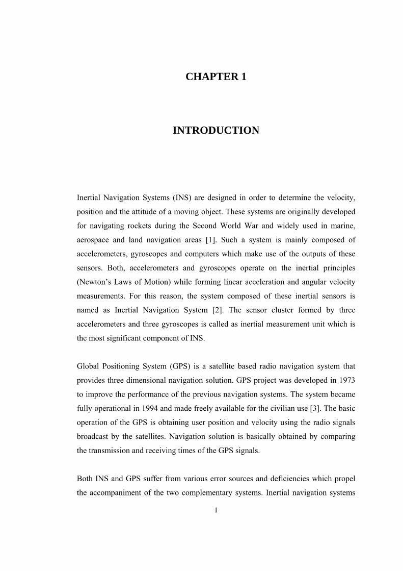
thesis work, a strapdown inertial navigation system is modeled. Diagram of the

internal structure of two systems can be seen in the figure below.

Figure 1 Inertial measurement units (Figure is adapted from [8])

  6

  7

2.1.3 IMU Technology

Basic operational principles and technological basis of accelerometers and

gyroscopes are discussed in this section.

2.1.3.1 Accelerometer Technology

Most of the accelerometers are based on force feedback or vibrating beam

technology. Both technologies share the same principle of measuring the force acting

on a proof mass instead of the vehicle [9].

2.1.3.1.1 Force Feedback Accelerometer

These types of accelerometers are also called as “pendulous mass”. A proof mass is

connected to the accelerometer case by the help of a pendulous arm. The proof mass

is made free to move only in the input axis direction by supporting it with a hinge in

two dimensions. Acceleration of the vehicle causes a force to act on the proof mass

which in turn results in a deflection in the position of the proof mass. An external

force which is proportional to the acceleration is required to stabilize the proof mass.

The deflection of the proof mass is detected by a pick-off system. The signal

generated by this system is used in a torquer system in order to move the proof mass

back to its null position. The force applied by the torquer system is proportional to

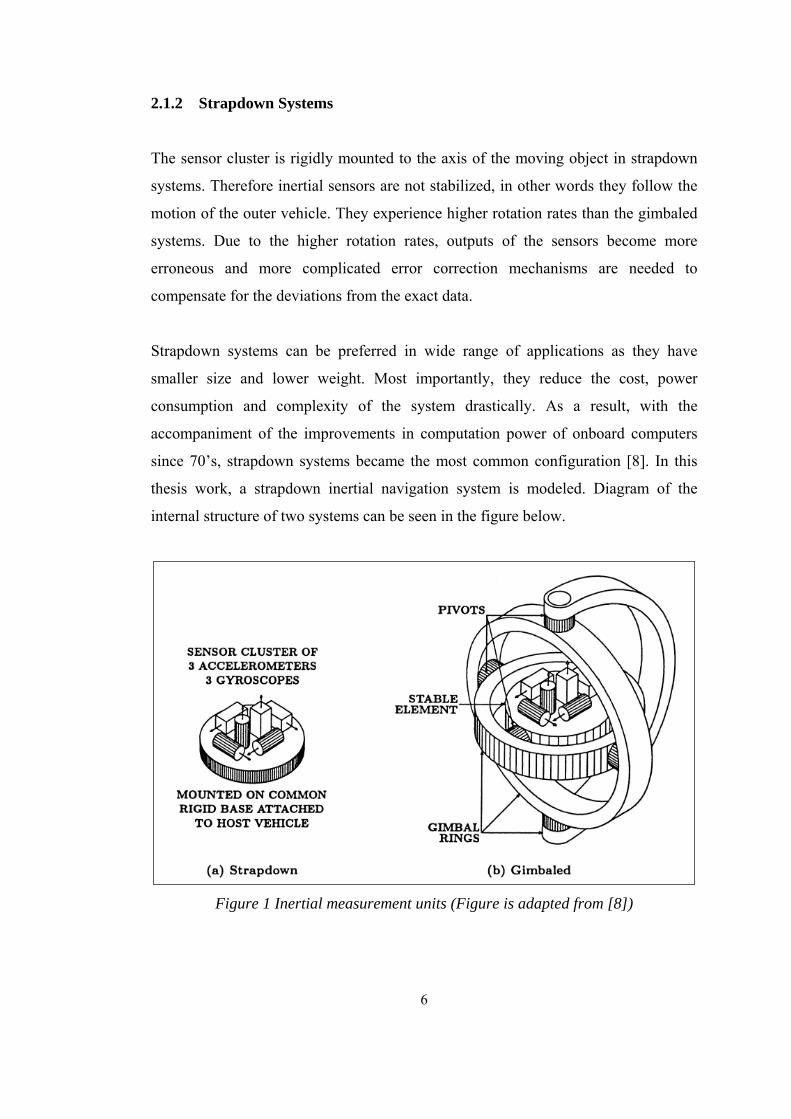
the acceleration of the host system [10]. A simple schematic of a force feedback

accelerometer can be seen in Figure 2

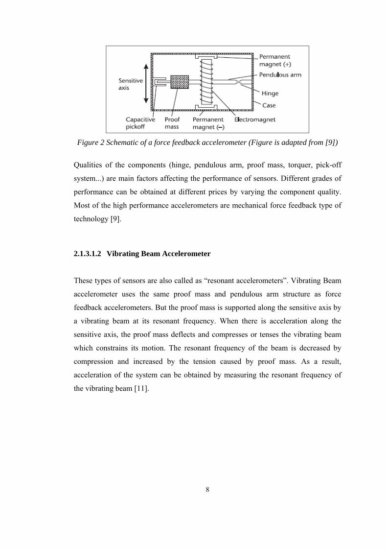
Figure 2 Schematic of a force feedback accelerometer (Figure is adapted from [9])

Qualities of the components (hinge, pendulous arm, proof mass, torquer, pick-off

system...) are main factors affecting the performance of sensors. Different grades of

performance can be obtained at different prices by varying the component quality.

Most of the high performance accelerometers are mechanical force feedback type of

technology [9].

2.1.3.1.2 Vibrating Beam Accelerometer

These types of sensors are also called as “resonant accelerometers”. Vibrating Beam

accelerometer uses the same proof mass and pendulous arm structure as force

feedback accelerometers. But the proof mass is supported along the sensitive axis by

a vibrating beam at its resonant frequency. When there is acceleration along the

sensitive axis, the proof mass deflects and compresses or tenses the vibrating beam

which constrains its motion. The resonant frequency of the beam is decreased by

compression and increased by the tension caused by proof mass. As a result,

acceleration of the system can be obtained by measuring the resonant frequency of

the vibrating beam [11].

  8

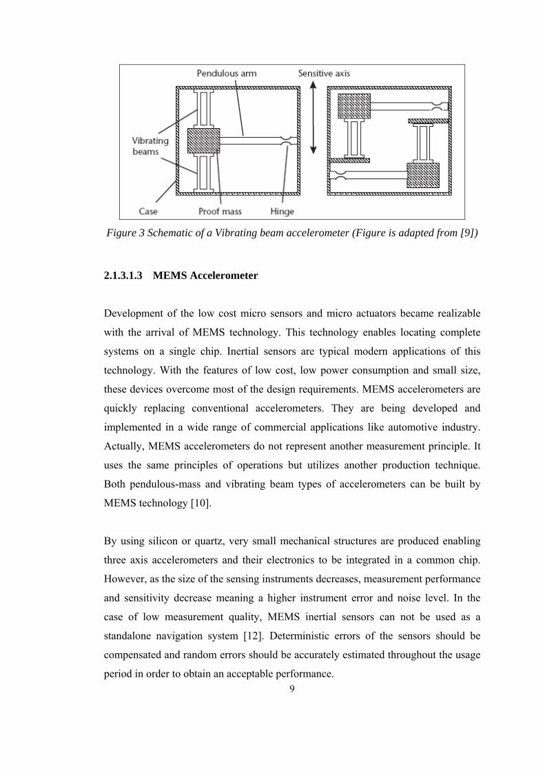
Figure 3 Schematic of a Vibrating beam accelerometer (Figure is adapted from [9])

2.1.3.1.3 MEMS Accelerometer

Development of the low cost micro sensors and micro actuators became realizable

with the arrival of MEMS technology. This technology enables locating complete

systems on a single chip. Inertial sensors are typical modern applications of this

technology. With the features of low cost, low power consumption and small size,

these devices overcome most of the design requirements. MEMS accelerometers are

quickly replacing conventional accelerometers. They are being developed and

implemented in a wide range of commercial applications like automotive industry.

Actually, MEMS accelerometers do not represent another measurement principle. It

uses the same principles of operations but utilizes another production technique.

Both pendulous-mass and vibrating beam types of accelerometers can be built by

MEMS technology [10].

By using silicon or quartz, very small mechanical structures are produced enabling

three axis accelerometers and their electronics to be integrated in a common chip.

However, as the size of the sensing instruments decreases, measurement performance

and sensitivity decrease meaning a higher instrument error and noise level. In the

case of low measurement quality, MEMS inertial sensors can not be used as a

standalone navigation system [12]. Deterministic errors of the sensors should be

compensated and random errors should be accurately estimated throughout the usage

period in order to obtain an acceptable performance.   9

  10

In the scope of this study, MEMS accelerometers are selected as the linear

acceleration measurement source and modeled accordingly.

2.1.3.2 Gyroscope Technology

Gyroscope technology is more complicated and more diverse than accelerometers.

There have been many different solutions for the design and production of

gyroscopes. Gyroscope technology can be discussed in four main types namely

spinning mass, optical, coriolis and MEMS gyroscopes [10]. Also there are two types

of optical gyroscopes, that is ring laser and fiber optic gyroscopes, using the same

principle of operation but different technological basis. All of these technologies are

handled separately in the following parts.

2.1.3.2.1 Spinning Mass Gyroscope

Gyroscopic theory is the fundamental method of measuring rotation of a body

without using an external reference [10]. When a spinning mass is rotated around its

input axis perpendicular to its spin axis, a reaction will take place in the third axis

which is perpendicular to both. The amount of this reaction is an indicator for the

rate of input rotation. This principle forms the basis for all mechanical gyroscopes

[10].

There exist different types of spinning mass gyroscopes such as dynamically tuned

gyroscope, electrostatically suspended gyroscope, magnetically suspended gyroscope

etc. A dynamically tuned gyroscope eliminates the movement in the reaction axis by

using an electrical rebalance loop. The input rotation rate is proportional to the

amount of required current for balancing the spinning mass. Different gyroscope

performances can be obtained at different prices depending on the quality of control

electronics, spin motor and torquers [9].

  11

2.1.3.2.2 Ring Laser Gyroscope

RLG consists of a triangular laser cavity with mirrors located at the vertices of closed

loop with at least three arms. A beam of laser is split into two beams, one of which

travels in the clockwise direction and the other in the counter-clockwise direction.

Mirrors at the vertices are used to form a continuous light path. Laser beams

generated travel around this path being reflected from each mirror, and return to its

initial starting point. In case of the sensor being stationary, both beams have the same

frequency. When the gyro rotates at some angular rate, optical path lengths change,

i.e., the distance traveled by the beam travelling in the opposite direction of the

rotation becomes shorter than the other one. The frequency of each beam changes to

maintain the resonant condition. This results in a phase difference between two

travelling waves. This phenomenon is called “Sagnac Effect”. The phase shift can be

measured by an interferometer. This output is proportional to the rate of rotation

[11].

The drawback of this technology is the laser lock phenomena. At low rotation rates,

the phase difference measured can be equal to zero as the result of back scattering.

This causes the beams to synchronize and travel at the same rates in the lock-in state.

At this state, the device will not accurately track its angular position over time

meaning that no measurements are taken. One of the methods to lessen this problem

is using mechanical oscillation. Angular vibrations are applied to the whole laser

cavity at high frequency and low amplitude through small angles. Drawback of this

method is an increase in size, weight and complexity of the system. The output

should be compensated optically or electronically for the oscillatory motion. There

are no moving parts in RLG structure meaning that there is no friction. Therefore

there will not be inherent drift terms, which is an advantage of the system.

Furthermore the entire unit is compact, light weighted and virtually indestructible.

The primary disadvantage of RLG technology is the requirement for polishing the

laser blocks and difficulties in producing the mirrors. High technology methods must

be used to produce the mirrors that increase the cost of the device. RLG technology

is still advancing, and it is at the practical limits of this technology [13].

2.1.3.2.3 Fiber Optical Gyroscope

Its principle operation depends on measuring the “Sagnac Effect” as in the case of

RLG. An external laser source exists in the FOG which generates travelling beams

both in the clockwise and in the counter-clockwise directions. In this setup, the light

waves travel in a fiber-optic cable. When the device experiences inertial rotation, the

distances travelled by two counter waves become different due to the sagnac effect.

This operation results in two different frequencies for two beams which mean a

phase difference between the laser beams. The output phase difference measured is

proportional to the rotation rate of the device [11].

Meanwhile, temperature changes and accelerations may disrupt the structure of the

optical fiber. This is one of the sources of error which should be minimized by using

design techniques. On the other hand fiber optic gyroscopes do not include mirrors or

gas in their internal design. Furthermore, lock-in phenomena is not inherent in FOG

technology unlike the RLG. These properties make the FOG technology cheaper

compared to RLG. In these days FOGs are replacing RLGs in the lower performance

tactical and commercial applications. Improvements in the FOG performance will

make it possible to use these devices in strategic applications with performance

requirements of 0,001 deg/h [10]. In the implementation of FOG; fiber-optic sensing

coil, a light source and a photo detector is used. In the figure below, internal

structures of two types of laser gyros (RLG, FOG) can be seen.

Figure 4 Basic components of laser gyroscopes (Figure is adapted from [8])

  12

  13

By the help of developments in the FOG technology, Interferromagnetic Fiber

Optical gyroscope (IFOG) is invented. This device has brought substantial increases

in the performance of gyroscopes. This technology has been used in many lower

grade applications as unmanned vehicles, stabilization systems etc. [8]. Measurement

accuracy of IFOGs is approaching to RLGs but due to high prices, it is not used

widely. However with increasing industrial investments, the costs will decrease and

IFOG is expected to replace RLG in high performance applications. With the

implementation of IFOG technology, integrated guidance and navigation systems

have the potential of having very low cost with high reliability and suitability for a

wide range of military and commercial applications [13].

2.1.3.2.4 Coriolis Gyroscope

Coriolis gyroscopes are also called as vibratory gyroscopes. In this type of sensors,

there exists an element which undergoes a simple harmonic motion in a plane. The

shapes of this vibrating element may be tuning fork, ring, hemisphere, cylinder,

spring, beam or pair of beams [9]. All types of these gyroscopes have the same

principle of operation, which can be summarized as detecting the coriolis

acceleration of the vibrating element when it is subject to a rotation. A sinusoidal

vibration is induced in a plane perpendicular to the vibration of the element when the

gyroscope is rotated. The amount of the induced vibration is proportional to the

rotation rate. Most of the coriolis gyroscopes have low performance specifications

with a low price. Hemispherical resonator gyroscope is an exception that it can

indeed offer high performance [10].

2.1.3.2.5 MEMS Gyroscope

As stated in section 2.1.3.1.3 about MEMS accelerometers, MEMS gyroscopes do

not represent a different measurement principle. They use the same principles of

operations but utilize another production technique. MEMS gyroscopes are generally

based on coriolis principles discussed in section 2.1.3.2.4. These gyroscopes are

  14

produced in very small sizes and micro-machined directly on silicon or similar

substrates. It is noted that better performances can be obtained by using quartz rather

than silicon substrates [9]. Basic advantages of this technology are its mass

production capability, very low cost with high quantity, very small size, minimal

power requirements and resistance to very high shock. In the context of this thesis, a

MEMS gyroscope with moderate performance is modeled.

2.1.4 IMU Error Sources

The outputs of the inertial sensors exhibit definite types of errors to some extent

depending on their performance. Bias, scale factor, misalignment and noise are the

basic systematic error sources of accelerometers and gyroscopes. Each of these error

sources has four different characteristics namely, a deterministic fixed component, a

temperature dependent component, a turn-on to turn-on component and an in-run

variation component [9]. First two deterministic components of sensor errors can be

compensated on the IMU processor by using the IMU calibration data. The

procedures for obtaining the calibration database for inertial sensors are clearly

defined by IEEE standards [14]. The remaining two other error components have a

stochastic behavior which determines the performance of the IMU. In the context of

this study, it is assumed that the deterministic errors of the IMU outputs are

compensated perfectly. Since post calibration performance of the IMU is major in

determining the inertial navigation performance, only stochastic errors are modeled

while forming the inertial data [9]. Stochastic error characteristics of accelerometers

and gyroscopes are discussed in detail.

2.1.4.1 Bias

Inertial sensor bias is defined as the constant error present in the average of the

sensor output over a specified time measured at specified operating conditions [14].

Bias error is independent of the underlying acceleration or angular rate of the sensor.

It is convenient to consider bias in two components as static and dynamic biases.

Static bias is also known as turn-on to turn-on bias or bias repeatability. This

component of the bias is set at the power up and it is constant throughout IMU

operation period. But it varies from run to run. Bias repeatability also includes

residual fixed bias remaining after the calibration of sensor [9]. The variation of the

bias repeatability can be represented by a Gaussian distribution and this component

can be modeled as a random constant as follows.

0

0bias accbias

bias gyrobias

a

(2.1)

Where , zero mean gaussian white noiseaccbias gyrobias

Dynamic bias is also known as in-run bias variation or bias stability. This component

of the bias varies over periods of order of a minute depending on the characteristics

of sensors. Bias stability also includes temperature dependent bias remaining after

the calibration of sensor. Typical value of the bias stability is about 10 percent of

bias repeatability [9]. Bias stability can be modeled as a first order Gaussian Markov

process.

2.1.4.2 Scale Factor

Scale factor is a parameter that is used to obtain acceleration or angular rate values

from the voltage outputs of accelerometers and gyroscopes. Scale factor is defined as

the departure of slope of the input-output curve of an inertial sensor from unity after

the unit conversion by IMU [14]. The scale factor errors of the accelerometers and

gyroscopes are proportional to acceleration and angular rates along the sensitive axis

respectively. Similar to bias, it is convenient to separate scale factor as static and

dynamic components.

Static component of the scale factor, namely scale factor repeatability is set at the

power up of the instrument and remains constant throughout IMU operation period.

It also includes the residual error left after the calibration of sensor. Scale factor

repeatability can be modeled as a random constant [9].

  15

  16

Dynamic component of the scale factor, namely scale factor stability is the dual of

bias stability. This component includes temperature dependent scale factor error

remaining after the calibration of sensor and represents the variation of the scale

factor error over the operating periods. Scale factor stability can also be modeled as a

first order Gaussian Markov process [9].

2.1.4.3 Misalignment

Because of the manufacturing limitations, sensitive axis of the inertial sensors cannot

be placed orthogonally. This makes each accelerometer and gyroscope sensitive to

the accelerations and angular rates along other axis which results in a cross-coupling

error. Scale factor and misalignment errors are unitless quantities which are typically

expressed in parts per million (ppm). Misalignment errors can be modeled as random

constants [7].

2.1.4.4 Noise

Random noise is an additional error resulting from the internal structure of inertial

sensors and sensor electronics. In general, random noise is a non-systematic,

stochastic process which cannot be compensated by using deterministic models.

Random noise of the inertial sensors can be modeled as zero mean additive white

noise. Random noise of the accelerometers and gyroscopes is generally described as

velocity random walk and angular random walk respectively. Noise on the

accelerometer measurements is integrated to obtain velocity random walk. Similarly,

noise on the gyroscope measurements is integrated to obtain angular random walk.

Magnitudes of the random walk process are proportional to the square root of the

integration time [9].

2.1.5 IMU Error Model

Accelerometers and gyroscopes exhibit further error characteristics such as bias

instability, g-dependent bias, g-square dependent bias, scale factor nonlinearity,

quantization noise etc. [9]. But these errors have negligible effect on the system

performance for a short period of operation time in the order of a few minutes and

they are out of scope of this study. The major error sources which have significant

contribution to the growth of errors in inertial navigation systems are bias

repeatability, scale factor repeatability, misalignment and random noise [4]. In the

simulations, first three parameters are set randomly at the beginning of each run and

held constant through that individual run. Random noise is generated at each time

step by randomly sampling from a zero mean Gaussian distribution whose standard

deviation is determined by the sensor specifications. Bias and scale factor stability

errors are not modeled since the simulation time is comparable with the correlation

time of these errors. The mathematical models, constituted in order to represent

realistic IMU errors by injecting predefined errors to the reference accelerometer and

gyroscope outputs are given in equations (2.2) and (2.3) respectively.

  17

x

z

w

1 1 0 0

1 0 1 0

1 0 0 1

b acc acc acc b acc accx x xy xz x xb acc acc acc b acc acc

y y yx yz y y yacc acc acc b acc accbz zx zy z zz

f b M M f S

f b M M f S w

b M M f S wf

(2.2)

Where , , , , ,b b acc acc acc accf f b M S w stand for reference acceleration, accelerometer

sensed acceleration, bias, misalignment, scale factor and noise parameters for

modeled accelerometer respectively.

1 1 0 0

1 0 1 0

1 0 0 1

b gyro gyro gyro b gyro gyrox x xy xz x x xb gyro gyro gyro b gyro gyroy y yx yz y y yb gyro gyro gyro b gyro gyroz z zx zy z z z

b M M S

b M M S w

b M M S w

w

(2.3)

Where , , , , ,g g gyro gyro gyro gyrob M S w stand for reference angular rate, gyroscope

sensed angular rate, bias, misalignment, scale factor and noise parameters for

modeled gyroscope respectively.

  18

2.2 Inertial Navigation System (INS) Dynamics

Main objective of the inertial navigation systems is obtaining position, velocity and

attitude information of the host platform. While constituting this navigation

information, onboard computer of the INS makes use of inertial data collected from

IMU, gravity data obtained from the Earth model and gravity model. Collected data

is processed by the help of kinematic INS mechanization equations and desired

inertial solution is acquired. In this section of the thesis, dynamics of the inertial

navigation system is discussed in detail.

2.2.1 Coordinate Frames

A coordinate frame is a reference that provides an origin and a set of axis in three

dimensional space for a moving object [9]. Defining required number of orthogonal

and right handed frames is the fundamental process of navigation. While navigating

in the vicinity of the Earth, velocity and position with respect to the Earth are the

main outputs [8]. At the same time, measurements of IMU are referenced to a non-

rotating inertial frame expressed in body axis of the vehicle. Therefore it is

customary to define the coordinate frames before considering the navigation

equations in order to prevent any confusion.

2.2.1.1 Inertial Frame (I-Frame)

Origin of the inertial frame is the centre of the Earth and its axes are non-rotating

with respect to the fixed stars. Z-axis of the inertial frame is coincident with the

Earth’s polar axis (z-axis).

2.2.1.2 Earth Frame (E-Frame)

Origin of the Earth frame is the center of the Earth and its axes are fixed with respect

to the Earth (rotating around the Earth’s polar axis with Earth rate). X-axis of the

  19

Earth frame points to the Greenwich meridian from the center of the Earth. Its Z-axis

is coincident with the Earth’s polar axis. Y-axis of the Earth frame is defined along

the equatorial plane forming a right handed orthogonal set with X-axis and Z-axis.

2.2.1.3 Navigation Frame (N-Frame)

Origin of the Navigation frame is at the center of navigation system which moves

with the host platform. It is a locally level geographic frame whose X, Y, Z axes are

aligned with the directions of north, east and down respectively.

2.2.1.4 Body Frame (B-Frame)

Origin of the body frame is at the center of navigation system. Orthogonal axes of

the body frame are aligned with roll, pitch and yaw axes of the navigating platform.

X-axis of the body frame is forward along the longitudinal axis of the navigating

platform, Z-axis is directed downward and Y-axis is defined towards right side of the

navigating platform forming a right handed orthogonal set with X-axis and Z-axis.

2.2.2 Earth Model

Since velocity and position with respect to Earth are the main outputs while

navigating in the vicinity of the Earth [8], it is required to define an Earth model

which makes realistic assumptions regarding the shape of the Earth. In most of the

navigation systems, Earth is modeled as an ellipsoid which is defined by two radii

[9]. The equatorial radius Ro is defined as the length of semi-major axis which is

equal to the radius of the Earth’s equatorial plane. Polar radius Rp is defined as the

length of semi-minor axis which is equal to the distance from earth center to either

pole.

In accordance with this model, the following parameters are defined in the WGS84

standards as given below. The ellipsoid is represented by the equatorial radius and

the flattening. Other Earth related parameters may be obtained using these two terms

[15].

0

0

1 2

6,378,137.0 : Length of semi-major axis

1 : Length of semi-minor axis

1 298.257223563: Flattening of the ellipsoid

e = 2 : Major eccentricity of the ellipsoid

p

R m

R R f

f

f f

(2.4)

A meridian of curvature and a transverse radius of curvature, which will be used in

defining the rates of change of latitude and longitude, may also be derived in

accordance with the ellipsoidal definition of the Earth [8].

20

3 22 2

01 22 2

1:Meridian radius of curvature

1 sin

:Transverse radius of curvature1 sin

N

E

R eR

e L

RR

e L

(2.5)

For navigation purposes, rotation rate of the Earth is assumed as a constant according

to the WGS84 standards. Value of the Earth rate is given in the equation (2.6) [15].

57.292115 10ie rad s (2.6)

Rotation of the Earth is in counter-clockwise direction around Z-axis of E-frame.

Earth rotation vector can be expressed in E-frame as follows.

0 0TE

IE IE (2.7)

Earth rotation vector can be expressed in N-frame as a function of geodetic latitude.

cos 0 sinTN

IE IE IEL L (2.8)

2.2.3 Gravity model

A relatively simple model of acceleration constituted by gravity at the ellipsoid as a

function of latitude is given by WGS84 datum as in the Equation (2.9). This is a

gravity field model called Somigliana. It is assumed that the gravity vector is

  20

perpendicular to the predefined ellipsoid and its direction is downwards through the

third axis of the N-frame [9].

2

20 2 2

1 0.001931853sin9.7803253359

1 sin

Lg L m

e L

s (2.9)

The variation of the gravitational field with height can be modeled using a scaling

parameter which is a function of latitude and height above the ellipsoid as follows.

2

02,e

eS

eeS

r Lg L h g L

r L h

(2.10)

22 2 2cos 1 sin : Geocentric radiuseeS Er L R L e L (2.11)

Acceleration due to gravity which is also called “plumb-bob gravity” is composed of

gravitational acceleration and centripetal acceleration [16].The formulas given above

define magnitude of the acceleration due to gravity. Since the direction of this

acceleration is downwards perpendicular to the predefined ellipsoid, vector form of

the plumb-bob gravity can be represented in N-frame as given in equation (2.12).

0 0 ,TN

pg g L h (2.12)

2.2.4 INS Mechanization

This section of the thesis focuses on the equations derived for obtaining navigation

solution, namely attitude, velocity and position, using linear acceleration and angular

rate outputs of IMU’s. Figure 5 shows a schematic of operations utilized in inertial

navigation processing.

  21

Bf

BIBw

Nf

NBC

,

, ,

N NBV C

L h

Npg

Figure 5 Schematic of the INS mechanization equations

After the initialization of navigation states, attitude computation is done in order to

transform the linear acceleration outputs of accelerometers from B-frame to N-frame.

Then using gravity model and coriolis correction, velocity and position computations

are done. INS mechanization is defined in the form of continuous time differential

equations. Equations for attitude, velocity and position mechanizations are given in

sections 2.2.4.1, 2.2.4.2 and 2.2.4.3 respectively.

2.2.4.1 Attitude Mechanization

Attitude is a significant parameter for strapdown inertial navigation processing since

transformation of vectors between different reference frames is utilized by using this

information. In the literature, there are miscellaneous methods for representing

attitude [16]. In the context of this thesis, coordinate transformation matrix, in other

words direction cosine matrix (DCM), is the selected notation for updating attitude

solution. For visualization and evaluation of the results, Euler angles are computed

from the DCM by a simple algorithm.

  22

Differential equation describing the rate of change of DCM that is used to transform

vectors represented in B-frame to vectors in N-frame is given below [17]. The

variables defined as x , xB NIB IN are skew-symmetric forms of the corresponding

vectors.

x xN N B NB B IB IN BC C C N (2.13)

Angular rates existing in the equation above are defined as follows.

cos 0 sin : Earth rate in N-frame

N N NIN IE EN

TNIE IE IEL L

(2.14)

Transport rate NEN is defined as the angular rate of the N-frame with respect to the

E-frame represented in the N-frame.

tan= cos sin

TTN NE E

ENE N E

VV VL L L

R h R h R h

L (2.15)

Where ,L stand for latitude, longitude and stand for east and north

components of . Initial value for this differential equation is obtained by using

initial Euler angles as follows.

,E NV V

NV

cos cos cos sin sin sin cos sin sin cos sin cos

cos sin cos cos sin sin sin sin cos cos sin sin

sin sin cos cos cos

NBC

(2.16)

Where , , are roll, pitch and yaw angles respectively. Initial values of these

angles are predefined depending on individual simulation trajectories.

2.2.4.2 Velocity Mechanization

As stated before, inertial navigation deals with the velocity of a moving object with

respect to the Earth. Since position solution is expressed in curvilinear coordinates by

latitude, longitude and altitude; velocity solution is supposed to be expressed in the

N-frame. At the same time, linear accelerations are measured with respect to I-frame

  23

and represented in B-frame. Therefore, starting from the I-frame, differential

equations for velocity mechanization are derived in I-frame, E-frame and N-frame in

turn [18].

Velocity in I-frame:

I I I I I IIE IE IEV f g r V I (2.17)

Velocity in E-frame:

2E E E E E EIE IE IEV f g r V E (2.18)

Velocity in N-frame:

2N N N N N N NIE IE IE ENV f g r V N

B

(2.19)

By substituting N NBf C f and plumb-bob gravity vector, conclusive equation for

N-frame velocity mechanization is obtained.

2N N B N N NB p IE ENV C f g V N (2.20)

2.2.4.3 Position Mechanization

Position solution of inertial navigation systems is generally expressed in curvilinear

coordinates by latitude, longitude and altitude for its simplicity and

comprehensibility. The rate of change of the curvilinear position can be expressed as

follows [19].

; ; N ED

N E

V VL h V

R h R h

(2.21)

Where; stand for the north, east and down components of the N-frame

velocity vector respectively. Definitions of are given in the Earth model

equation

, ,N E DV V V

,N ER R

(2.5).

  24

In order to transform vectors defined in the N-frame to E-frame, a DCM is formed

which is function of latitude and longitude. For instance, the Earth rate vector

represented in E-frame is transformed to the N-frame via transpose of this DCM

[19].

sin cos sin cos cos

sin sin cos cos sin

cos 0 sin

EN

L

C L L

L L

(2.22)

A summary of the INS mechanization equations is given in the table below.

Table 1 INS mechanization equations

Attitude x xN N B NB B IB IN BC C C N

Velocity 2N N B N N NB p IE ENV C f g V N

Position ; ; N ED

N E

V VL h V

R h R h

2.2.5 INS Error Model

In the context of this thesis, an error state system model will be constituted for the

integration of INS and GPS. Position, velocity, attitude errors and inertial sensor

biases are selected as the state space variables. Therefore nonlinear equations for

position, velocity and attitude given in the previous section need to be linearized

about the most recent navigation solution. For this linearization operation, nonlinear

equations are perturbed for the state space variables [9]. In the derivation step of this

model, second order terms in the error quantities are dropped [19].

2.2.5.1 Attitude Error Model

For the attitude errors, small angle attitude error model is utilized. The attitude

mechanization equation [equation (2.13)] is linearized with respect to the state space

variables and the following results are obtained [9].

  25

x N B N BIN IN BC IB (2.23)

Where; is the attitude error present in the state estimate.

B IB is the gyroscope error vector represented in the B-frame.

NIN is the error in the angular rate of the N-frame with respect to the I-frame

which is composed of earth rate error and transport rate error as given below.

N N NIN IE EN (2.24)

Earth rate error NIE is obtained by perturbing the Earth rate N

IE by latitude error

L . Assuming that perturbation of the Earth rate is equal to zero

sin 0 cosTN

IE L L L L

(2.25)

Transport rate error is similarly obtained by perturbing NEN N

EN by four of the

state space variables EV , NV , h , L .

2

2

2 2

tantan

cos

E E

E E

N N NEN

N N

E EE

E EE

V Vh

R h R h

V Vh

R h R h

V L VLV h

R h R h LR h

L

(2.26)

Attitude error model can be represented in state space form as follows. Definitions

for the elements of the state space are given in Section 2.2.5.4.

N BP V B I

P

F F F V C

B

(2.27)

  26

2.2.5.2 Velocity Error Model

Similarly, velocity error model is obtained by perturbing the velocity mechanization

equation given in the equation (2.20) by state vectors, Earth rate and transport rate

errors. The rate of change of velocity error is given below as a function of state

variables and gravity error [9].

022 2N N B N B N N N N N N

B B IE EN IE EN eeS

g LV C f C f V V

r Lh

(2.28)

Velocity error model can be represented in state space form as follows. Definitions

for the elements of the state space are given in section 2.2.5.4 state space error

model.

NVP VV VV F P F V F (2.29)

2.2.5.3 Position Error Model

Analogous to velocity error model, position error model is obtained by perturbing the

position mechanization equation given in the equation (2.21) by position and velocity

error states [9].

2

2

1

tan1

cos cos cos

NN

N N

E EE

E E E

D

VL V h

R h R h

V L VV L

R h L R h Lh

R h L

h V

(2.30)

Position error model can be represented in state space form as follows. Definitions

for the elements of the state space are given in section 2.2.5.4 state space error

model.

PP PV P

P

P F F F V

(2.31)

  27

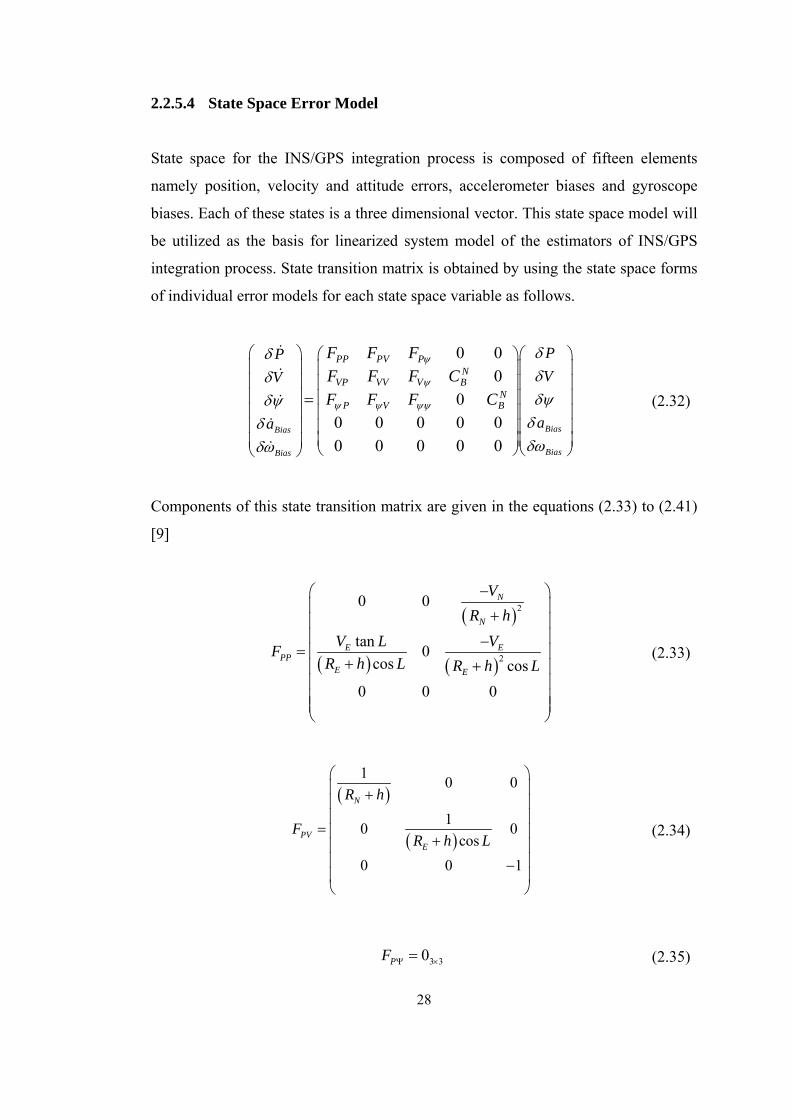
2.2.5.4 State Space Error Model

State space for the INS/GPS integration process is composed of fifteen elements

namely position, velocity and attitude errors, accelerometer biases and gyroscope

biases. Each of these states is a three dimensional vector. This state space model will

be utilized as the basis for linearized system model of the estimators of INS/GPS

integration process. State transition matrix is obtained by using the state space forms

of individual error models for each state space variable as follows.

0 0

0

0

0 0 0 0 0

0 0 0 0 0BiasBias

BiasBias

PP PV PN

VP VV V BN

P V B

PP

VV

aa

F F F

F F F C

F F F C

(2.32)

Components of this state transition matrix are given in the equations (2.33) to (2.41)

[9]

2

2

0 0

tan0

cos cos

0 0 0

N

N

E EPP

E E

V

R h

V L VF

R h L R h L

(2.33)

10 0

10

cos

0 0

N

PVE

R h

FR h L

0

1

(2.34)

3 30PF (2.35)

  28

2 2

2 22

22

22

2 2

tan2 cos 0

cos

tan2 cos 2 sin 0

cos

2 sin 0

N DE EE

E E N

N E E N E DVP N D

E E

NEE

E N

V VV VV L

R h L R h R h

V V V V L V VF V L V L

R h L R h

VVV L

R h R h

L

(2.36)

2 tan2 sin

tantan2 sin 2 cos

2 22 cos 0

ND E

N E N

N DE EVV

E E E

N E

N E

VV V LL

R h R h R h

V L VV L VF L L

R h R h R h

V VL

R h R h

(2.37)

0

0 ;

0

N xD EN

V D N E B

E N D z

y

f ff f

F f f f C

f f f

f

f

(2.38)

2

2

22

sin 0

0 0

tancos 0

cos

E

E

NP

N

E E

E E

VL

R h

VF

R h

V VL

R h L R h

L

(2.39)

10 0

01

0 0 ; 0

0tan

0 0

ED E

V DN

E N

E

R h

F FR h

L

R h

N

(2.40)

  29

Where T N N N

N E D IN IE EN

sin0 sin

cos

sinsin 0 cos

cos

cos 0

NE

E N

E E

E E

N E

N E

VV LL

R h L R h

V L VF L

R h L R h

V VL

R h R h

L

(2.41)

  30

  31

CHAPTER 3

3 GLOBAL POSITIONING SYSTEM (GPS)

The global positioning system is a satellite based navigation system that provides the

users three dimensional position and velocity solution by using passive radio signals.

Accurate time information is also provided in addition to the navigation solution

when there is an unobstructed line of sight to four or more satellites. GPS project was

developed in order to get through the deficiencies of the previous navigation systems

in 1973 by U.S. Department of Defense. The system became fully operational in

1994 and made freely available for the civilian use [3]. Several improvements and

modernizations are made to the system in order to meet the military and civilian

users' needs. There are ongoing studies which aim to increase performance and

accuracy of the system [10].

The basic operation of the GPS is obtaining user position and velocity using radio

navigation signals broadcast by the orbiting satellites. These signals include the

position and velocity information of each satellite and the time of transmission of the

signal from the satellite. By comparing the transmission and receiving times of the

GPS signals, the range between satellites and the GPS receiver antenna is measured

assuming that the signal travels with the speed of light. Geometrically, position of the

user should be on a sphere centered at the corresponding satellite with a radius

defined by the range information obtained. Each ranging data gathered from

individual satellites defines a similar sphere for the position of the user. When two

satellites are available, position solution is confined on a circle formed by the

intersection of two spheres. By using the information from a third satellite, two

  32

possible points are determined to define the user position. Therefore, signals from at

least four satellites are required in order to obtain navigation solution of a GPS user.

When there exists an obstruction of line of sight to the satellites or a signal loss

resulting in access to less than four satellites, standalone GPS cannot provide

navigation solution to its users [19].

In this chapter, fundamental characteristics of the GPS are considered first. Then

techniques for obtaining the GPS navigation solution for position are investigated.

After defining the sources of measurement errors, a nonlinear measurement model is

obtained at the end of the chapter.

3.1 GPS Fundamentals

GPS consists of three main segments namely the space segment, the control segment

and the user segment. The space and control segments are maintained and operated

by the US Air Force [20]. The user segment consists of GPS receiver and receiver

antenna which are commercial off-the-shelf products.

The space segment is composed of the GPS satellites which rotate in Earth centered

approximately circular orbits. The set of satellites in orbit providing the ranging

signals and data messages to the user segment is called the satellite constellation.

Standard constellation consists of twenty-four satellites which are positioned in six

orbital planes with four satellites in each plane [21]. The orbits are equally spaced

around the equatorial plane with a nominal inclination angle which provides an all-

day long global navigation capability. The subsystems of the satellites perform some

functions such as maintaining the solar panels pointing to the sun and satellites

pointing to the Earth [21].

The control segment is physically composed of the master control station, monitor

stations and the ground antennas. Basic operation of the control segment is

maintaining the orbital configuration of satellites, monitoring the health of satellites

and signals broadcast. Moreover, satellite clock corrections, ephemerides, almanac

  33

and other control parameter updates are sent to the constellation at least once per day

by the control segment. Command and control of the GPS constellation is provided

by the master control station centrally. All of the six monitor stations and four

ground antennas are also controlled remotely by the master control station [20].

The user segment comprises the GPS receiver and also the receiver antenna. The

radio frequency signals transmitted from GPS constellation are converted to

electronic signals by receiver antenna and processed by the receiver in order to

obtain position, velocity and time information. A GPS receiver processor consists of

two main components. First one is the ranging processor which determines the

transmission time of the received signal and forms the GPS observables. Second one

is the navigation processor which obtains GPS navigation solution by using the GPS

observables [9]. In the next section, basic operations used in the navigation processor

are summarized.

3.2 GPS Navigation Solution

In order to calculate the position of a GPS receiver, at least four satellites should be

available since there are four parameters to be determined to find the user position in

the E-frame; three parameters for X, Y, Z coordinates and receiver clock bias term.

In order to obtain these four unknowns four independent equations are needed.

Position calculations are done by using the ranging signals and data messages which

are acquired from individual GPS signals broadcast by the satellites [19].

Position computation of the receiver is done by making use of the pseudo range

observable which is obtained from the ranging signals. Pseudo range is the receiver

calculated erroneous range between each satellite and the receiver antenna. It is

obtained by comparing the transmission and receiving time of the GPS signals and

multiplying by the speed of light [22].

Pseudo ranges can be modeled as:

i r i iP t t c c (3.1)

Where; i stands for the number of satellite, i is the travelling time of the signal from

satellite i to the receiver, and c represents speed of light.

Atomic clocks in each satellite and clocks in the receivers do not run exactly aligned

with the true GPS time which is represented by . There exists a clock offset in

each clock of the satellites and the receiver. Clock offsets of the GPS satellites are

determined by the control segments and sent to each satellite. This correction term is

present in the data message broadcast by each satellite

GPSt

[9].

The clock offsets of GPS satellites and the receiver can be defined as:

: i'th satellite time

: receiver time

GPSi i

GPSr r

t t t

t t t

(3.2)

3.2.1 Measurement Equation

The most common algorithm used in the position calculations of receivers using

pseudo ranges is the least squares estimator (LSE) [23]. This method can easily be

used for over determined systems where the number of equations is more than the

number of unknowns. First of all, measurement equation for the GPS position should

be written in order to use LSE.

The geometric range between the satellites and the receiver can be defined as:

2 2

i i i iX X Y Y Z Z 2 (3.3)

Where , ,i i iX Y Z and correspond to ECEF position of the ith satellite and true

position of the GPS receiver respectively. ECEF positions and velocities of the

satellites are present in the data message broadcast by each satellite therefore these

variables are given.

, ,X Y Z

  34

By adding the measurement errors of the GPS receiver to the geometric range,

equation for the measured pseudo range can be obtained as follows:

i i r i i iP c t t T I ie (3.4)

Undefined variables in the measured pseudo range equation above can be clarified as

: Tropospheric delay

: Ionospheric delay

: Pseudo range measurement residual

i

i

i

T

I

e

Atmospheric delay parameters are included in the data message broadcast by each

satellite as correction terms. Definitions of these measurement error parameters are

given in detail in section 3.3.

Combining the geometric range equation with the previous equation, conclusive

expression for the measured pseudo range can be obtained as follows.

2 2 2

i i i i r i i iP X X Y Y Z Z c t t T I ie (3.5)

There are only four unknowns in the equation above, namely receiver position

and receiver clock bias, ,X Y Z rt .

3.2.2 Least Squares Estimate of The Navigation Solution

Measurement residual term should be minimized using the least square estimator

for obtaining the unknown receiver position. In order to use this estimator, the

nonlinear equation for the pseudo range measurement needs to be linearized for

receiver position coordinates and receiver clock bias as follows.

kie

, ,X Y Z

Starting point of the linearization can be chosen to be the center of the Earth as a rule

of thumb [23].

0 0 0, , 0,0,0X Y Z (3.6)

  35

The estimated user position is used as the linearization point of the next iteration.

After a number of iterations using the same GPS measurements, user navigation

solution is obtained.

Define geometric range function as,

  36

2 2, , i i i

2f X Y Z X X Y Y Z Z (3.7)

Define 1 1 1 0 0 0, , , ,X Y Z X X Y Y Z Z

First order Taylor series expansion of the function can be obtained as follows:

0 0 0 0 0 0 0 0 01 1 1 0 0 0

0 0 0

, , , , , ,, , , ,

f X Y Z f X Y Z f X Y Zf X Y Z f X Y Z X Y Z

X Y Z

(3.8)

After taking the partial derivatives, the first order linearized equation is obtained as:

0 0 0i i ii i r i r i i

i i i

X X Y Y Z ZP X Y Z c t t c t T

iI e

(3.9)

Where 2 2

i i i iX X Y Y Z Z 2

The equation for pseudo ranges can be written in matrix from as;

1i i ii i r i i i

i i i

r

X

YX X Y Y Z ZP c

Z

c t

it t T I e

(3.10)

Rearranging this equation in the standard form for LSE Ax b , the following result

is obtained. In this equation, n stands for the number of satellites. Therefore A is a

matrix 4n [23].

1 1 1

1 1 1 1 1 1 1 1 1

1

1

r

n n n n n r n n nr

n n n

X X Y Y Z ZX

P c t c t T I eY

ZnX X Y Y Z Z P c t c t T I e

c t

(3.11)

Note that, least squares estimation for the system Ax b is

12min || || minT T T

ie b Ax b Ax x A A

A b (3.12)

3.3 Measurement Errors

The essential measurements made by the GPS receivers are pseudo range and pseudo

range rates. These measurements are subject to time-correlated and noise like errors

[9]. Each of these errors will be defined and their effects to the GPS navigation

solution will be discussed in this section.

The satellite clock errors originate from the oscillator noise of the precise atomic

clocks. This source of errors can be calibrated by using the coefficients in the data

message. The residual clock error which depends on the stability of the satellite clock

and control segment's monitoring network results in about 1 meter of range error on

the average [24].

The ephemeris prediction errors arise due to the errors in the control segment's

prediction of the satellite positions. The effects of ephemeris errors vary with

different satellite geometries, but it results in an average range error of 0.45 meter

[9].

The ionosphere layer of the atmosphere refracts GPS signals due to its dispersive

medium. This refraction causes a delay in the carrier of the GPS signal. The effect of

ionospheric delay on range error changes with the time of the day and satellite

geometry.

  37

Troposphere is a nondispersive layer of atmosphere which extends about 12 km

above the Earth surface. The tropospheric delay can be corrected by using models

which are functions of elevation and height of the user. These corrections of the

troposhperic delay give up residual errors resulting in about 0.2m of range error in

pseudo range measurements [9].

Multipath error occurs when the GPS antenna receives reflected signals from a given

satellite in addition to the direct signals. In most cases, GPS signals are reflected

from the host body, ground, buildings and trees. These signals are always delayed

compared to the direct signals.

Modeling and evaluation of these separate error sources are not in the context of this

thesis. Therefore, measurement errors of GPS are modeled as additive zero mean

Gaussian noise for simplicity. The resulting measurement equation is as follows.

ky h x v (3.13)

Where 20,kv N and h x is the nonlinear measurement function defined in the

next section. Designation of the variance of the measurement noise 2 is

considered in section 4.3.

3.4 Nonlinear Measurement Model

In the tightly coupled INS/GPS integration architecture, which is discussed in

Section 4.2.2, pseudo range and pseudo range rate observables are used as GPS

measurements. The nonlinear equations relating the measurements to the state

variables are the geometric range and range rate functions.

2 2

1 , , i i ih X Y Z X X Y Y Z Z 2

(3.14)

2 2

2 , ,i i iX Y Z X X Y Y Z Zh V V V V V V V V V

2 (3.15)

  38

  39

Where and correspond to ECEF position and velocity of the

ith satellite. This information is acquired from the GPS data signal for each visible

satellite. and

, ,i i iX Y Z

, ,X Y Z

, ,i i iX Y ZV V V

, ,X Y ZV V V correspond to the estimated user ECEF position

and velocity. The estimated navigation solution can be obtained after the feedback

step involved in the error state Kalman filter implementation.

  40

CHAPTER 4

4 INS/GPS INTEGRATION

Inertial navigation systems exhibit relatively low noisy outputs which tend to drift

over time. A typical aviation grade INS errors grow at rates about 1-10 nmi/h (1.8-18

km/h) during normal operation [25]. Contrary to INS, GPS outputs are relatively

noisy but do not exhibit long-term drift [4]. Using both of these systems results in a

superior navigation performance than either alone. Integrating the outputs from each

sensor results in a system which can be visualized as a drift free INS. Benefits of

integrating these two navigation systems can be realized by first considering

advantages and disadvantages of individual systems. In section 4.1, benefits and

drawbacks of two systems are discussed in detail. The subsequent section focuses on

the INS/GPS integration architectures, namely loosely coupled, tightly coupled and

deeply coupled architectures. Each of these architectures determines the amount of

interaction of two separate systems and the attribute of data used in the integration

process.

4.1 Benefits and Drawbacks of Each System

Each of INS and GPS has a number of advantages and disadvantages. INS operation

is not dependent on outer signals or systems. It is a self-contained system operating

continuously in all external conditions and provides high bandwidth output at high

rates. Outputs of the INS, namely position, velocity and attitude, exhibit low short-

term noise. INS also provides linear acceleration and angular rates which are used by

stabilization and flight control systems [4]. On the other hand, as the instrument

  41

errors are continuously integrated in the INS mechanization equations, accuracy of

the navigation solution degrades with time. For a relatively long operation periods of

navigation, in the order of minutes, high performance INS’s are required which have

high cost about 100000$, high power consumption and large size restricting the

platform settlement [9].

In contrast to the INS, GPS is dependent on the signals broadcast by the satellites.

External conditions, namely weather conditions, visibility of the satellites, satellite

geometry, multipath of the signals and jamming have significant effects on the

performance of the navigation solution. Standalone GPS provides high long-term

position accuracy with limited errors to a few meters. Navigation solution of the GPS

includes just position and velocity of the platform. These navigation states are output

at very low rates, around 1-10Hz, and exhibit short-term high frequency noise.

Attitude solution, linear acceleration and angular rate signals are not provided by this

system. GPS signals are also subject to obstruction and interference which make the

system unreliable for continuous navigation. The benefits and drawbacks of the INS

and standard GPS are summarized in the following table for comparison [8].

Table 2 Benefits and drawbacks of INS and GPS Technical Properties INS GPS

Error propagation with

time Increases with time Limited errors in time

Attitude Solution Available Not availble

Flight control signals Available Not availble

Data rate High rate (100-1000 Hz) Low rate(1-10 Hz)

Bandwidth High bandwidth Low bandwidth

Interference Resistent Vulnerable

Dependency to environment Independent of the outer

world

Environment

dependent

Initial value assignment Not available Available

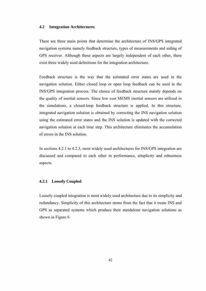
  42

4.2 Integration Architectures

There are three main points that determine the architecture of INS/GPS integrated

navigation systems namely feedback structure, types of measurements and aiding of

GPS receiver. Although these aspects are largely independent of each other, there

exist three widely used definitions for the integration architecture.

Feedback structure is the way that the estimated error states are used in the

navigation solution. Either closed loop or open loop feedback can be used in the

INS/GPS integration process. The choice of feedback structure mainly depends on

the quality of inertial sensors. Since low cost MEMS inertial sensors are utilized in

the simulations, a closed-loop feedback structure is applied. In this structure,

integrated navigation solution is obtained by correcting the INS navigation solution

using the estimated error states and the INS solution is updated with the corrected

navigation solution at each time step. This architecture eliminates the accumulation

of errors in the INS solution.

In sections 4.2.1 to 4.2.3, most widely used architectures for INS/GPS integration are

discussed and compared to each other in performance, simplicity and robustness

aspects.

4.2.1 Loosely Coupled

Loosely coupled integration is most widely used architecture due to its simplicity and

redundancy. Simplicity of this architecture stems from the fact that it treats INS and

GPS as separated systems which produce their standalone navigation solutions as

shown in Figure 6

Figure 6 Flowchart of loosely coupled architecture

Position and/or velocity information computed by GPS navigation filter is used as

the measurement of the integration filter in order to estimate the INS errors.

Standalone INS solution is corrected using the estimated error states and integrated

navigation solution is obtained

This architecture can be utilized with any commercial off-the-shelf INS and GPS

user equipment. Redundancy of this architecture stems from the fact that, in addition

to the integrated solution, each of the INS and GPS produces its independent

solution. This enables integrity monitoring of the utilized INS/GPS Kalman filter

[12].

4.2.2 Tightly Coupled

Tightly coupled integration eliminates the usage of cascaded filters unlike loosely

coupled integration. Therefore, correlation of the measurements in GPS navigation

filter is prevented. Instead of navigation solution of GPS, pseudo range and/or

pseudo range rates obtained from Doppler data is used as the measurements of

INS/GPS integration Kalman filter. Choice of these measurements brings

nonlinearity to the measurement model of the integration filter. Figure 7 shows the

flowchart of this architecture.

  43

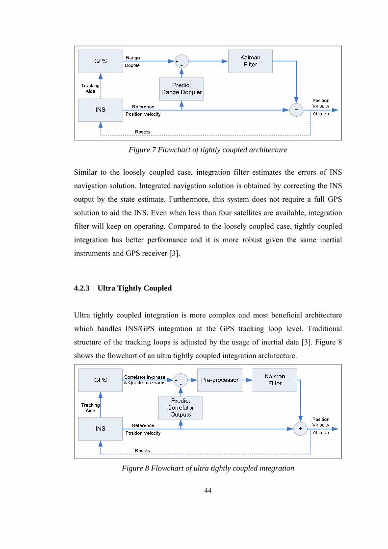
Figure 7 Flowchart of tightly coupled architecture

Similar to the loosely coupled case, integration filter estimates the errors of INS

navigation solution. Integrated navigation solution is obtained by correcting the INS

output by the state estimate. Furthermore, this system does not require a full GPS

solution to aid the INS. Even when less than four satellites are available, integration

filter will keep on operating. Compared to the loosely coupled case, tightly coupled

integration has better performance and it is more robust given the same inertial

instruments and GPS receiver [3].

4.2.3 Ultra Tightly Coupled

Ultra tightly coupled integration is more complex and most beneficial architecture

which handles INS/GPS integration at the GPS tracking loop level. Traditional

structure of the tracking loops is adjusted by the usage of inertial data [3]. Figure 8

shows the flowchart of an ultra tightly coupled integration architecture.

Figure 8 Flowchart of ultra tightly coupled integration

  44

This architecture can improve acquisition time and tracking performance of the GPS

signals. The most important profit of this method is its ability to operate at lower

signal to noise ratio levels. In this architecture, in-phase and quadrature samples of

the GPS correlators can be used as measurement for the INS/GPS estimator [26].

In the context of this thesis study, a tightly-coupled INS/GPS integration architecture

is utilized due to its higher performance than loosely coupled integration and relative

simplicity compared to ultra-tightly coupled integration.

4.3 IMU/GPS Specifications

In the context of this thesis, a MEMS accelerometer and a MEMS gyroscope based

low performance IMU is chosen as the basic component of the navigation system.

The utilized MEMS IMU, MTi is a commercial off-the-shelf stabilization grade

instrument produced by the Xsens Technologies Company. The performance

specifications of this unit are gathered from its datasheet issued by the company and

given in the following table.

Table 3 Specifications of the MEMS IMU Specifications Gyroscope Accelerometer

Bias repeatability 200 deg/ h 40 mg

Scale factor repeatability 1000 ppm 1000 ppm

Misalignment 0.1 deg 0.1 deg

Noise 0.05 deg/ /h hz 0.002 2/ /m s hz

  45

In order to obtain realistic results from the simulations, aiding measurement system

is also modeled using specifications of a commercial off-the-shelf GPS receiver. In

the process of forming GPS measurements, reference pseudo range and pseudo range

rate observables are calculated using reference satellite positions, velocities and

reference user position, velocity. Zero mean Gaussian random noise is added to the

reference pseudo range and pseudo range rate measurements to obtain realistic GPS

measurements. Standard deviation parameters of the Gaussian distributions are

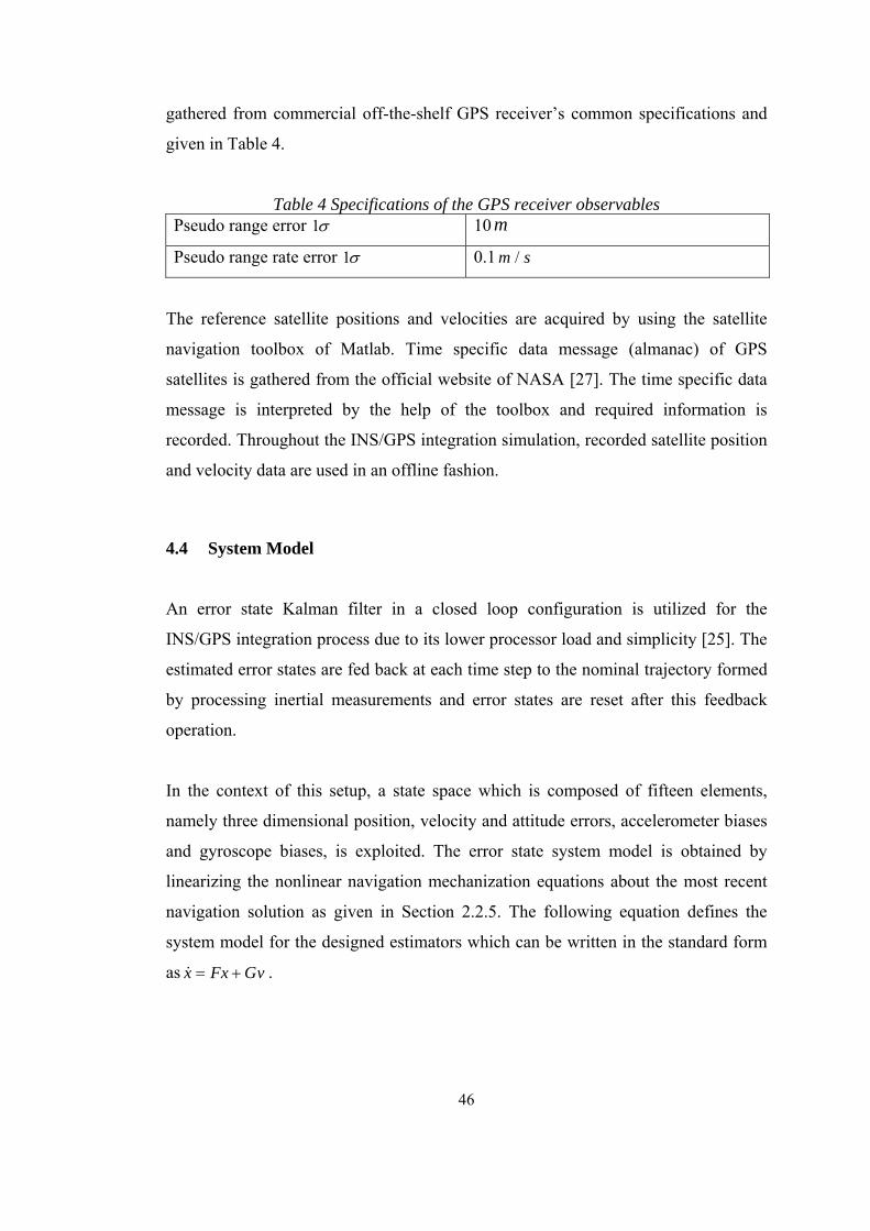
gathered from commercial off-the-shelf GPS receiver’s common specifications and

given in Table 4.

Table 4 Specifications of the GPS receiver observables Pseudo range error 1 10 m

Pseudo range rate error 1 0.1 /m s

The reference satellite positions and velocities are acquired by using the satellite

navigation toolbox of Matlab. Time specific data message (almanac) of GPS

satellites is gathered from the official website of NASA [27]. The time specific data

message is interpreted by the help of the toolbox and required information is

recorded. Throughout the INS/GPS integration simulation, recorded satellite position

and velocity data are used in an offline fashion.

4.4 System Model

An error state Kalman filter in a closed loop configuration is utilized for the

INS/GPS integration process due to its lower processor load and simplicity [25]. The

estimated error states are fed back at each time step to the nominal trajectory formed

by processing inertial measurements and error states are reset after this feedback

operation.

In the context of this setup, a state space which is composed of fifteen elements,

namely three dimensional position, velocity and attitude errors, accelerometer biases

and gyroscope biases, is exploited. The error state system model is obtained by

linearizing the nonlinear navigation mechanization equations about the most recent

navigation solution as given in Section 2.2.5. The following equation defines the

system model for the designed estimators which can be written in the standard form

as x Fx Gv .

  46

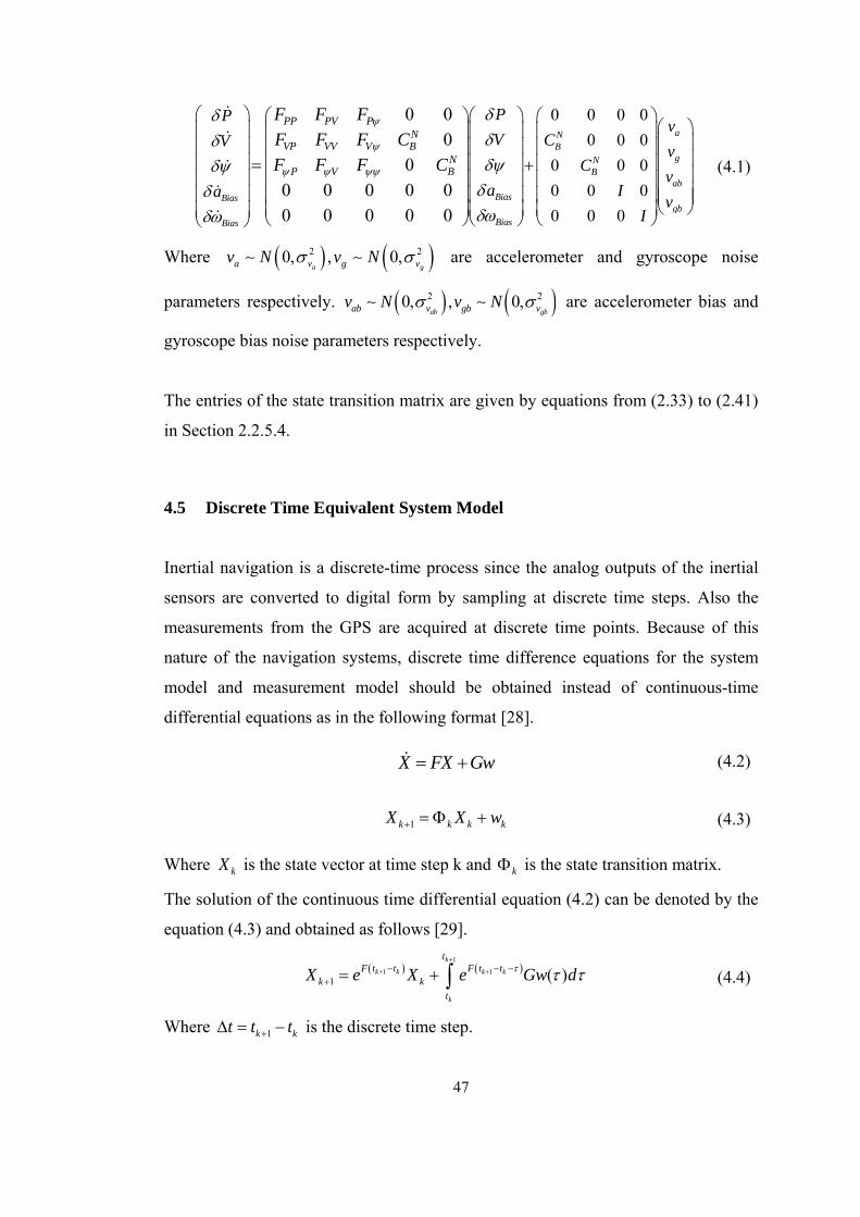
0 0 0 0

0 0 0

0 0 0

0 0 0

0 0 0

0 0

0

0

0 0 0 0 0

0 0 0 0 0

aNB

gNB

ab

BiasBiasgb

BiasBias

PP PV PN

VP VV V BN

P V B

PPv

V CVv

Cv

a Iav

I

F F F

F F F C

F F F C

(4.1)

Where 20, , 0,aa v gv N v N 2

gv are accelerometer and gyroscope noise

parameters respectively. 2 , 0,gbgb vv N 20,

abab vv N are accelerometer bias and

gyroscope bias noise parameters respectively.

The entries of the state transition matrix are given by equations from (2.33) to (2.41)

in Section 2.2.5.4.

4.5 Discrete Time Equivalent System Model

Inertial navigation is a discrete-time process since the analog outputs of the inertial

sensors are converted to digital form by sampling at discrete time steps. Also the

measurements from the GPS are acquired at discrete time points. Because of this

nature of the navigation systems, discrete time difference equations for the system

model and measurement model should be obtained instead of continuous-time

differential equations as in the following format [28].

X FX Gw (4.2)

1k k k kX X w (4.3)

Where kX is the state vector at time step k and k is the state transition matrix.

The solution of the continuous time differential equation (4.2) can be denoted by the

equation (4.3) and obtained as follows [29].

1

1 1

1 ( )k

k k k k

k

tF t t F t t

k k

t

X e X e Gw d

(4.4)

Where is the discrete time step. 1kt t t k

  47

Assuming that the system dynamics matrix F is constant over a time period of t ,

the state transition matrix can be simply obtained by matrix exponential of F t [28].

2

2!F t

k

F te I F t

(4.5)

The numerical evaluation of the discrete-time equivalent of process noise is more

difficult than the state transition matrix. The following method proposes a simplified

algorithm for the evaluation of the discrete-time process noise [28]. In this method,

the matrix exponential of the matrix A is evaluated at first.

0

T

T

F GWGA

F

1

0Ak

T

QB e

(4.6)

1*k kQ Q (4.7)

Where is the power spectral density matrix of the process noise and G is the

scaling matrix of the process noise defined in Equation

W

(4.2).

Then, by using the upper right and lower right parts of the matrix B, discrete-time

equivalent process noise matrix is obtained. kQ

4.6 Measurement Model

The nonlinear measurement functions relating the state space variables and GPS

measurements, namely pseudo range and pseudo range rates are given again in the

equations (4.8) and (4.9) respectively for the sake of completeness.

2 2

1 , , i i ih X Y Z X X Y Y Z Z 2

(4.8)

2 2

2 , ,i i iX Y Z X X Y Y Z Zh V V V V V V V V V

2 (4.9)

  48

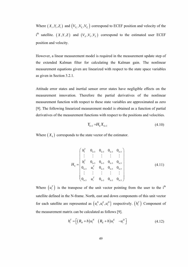
  49

Where and correspond to ECEF position and velocity of the

ith satellite.

, ,i i iX Y Z , ,i i iX Y ZV V V

, , ZX Y and , ,X Y ZVV V correspond to the estimated user ECEF

position and velocity.

However, a linear measurement model is required in the measurement update step of

the extended Kalman filter for calculating the Kalman gain. The nonlinear

measurement equations given are linearized with respect to the state space variables

as given in Section 3.2.1.

Attitude error states and inertial sensor error states have negligible effects on the

measurement innovation. Therefore the partial derivatives of the nonlinear

measurement function with respect to these state variables are approximated as zero

[9]. The following linearized measurement model is obtained as a function of partial

derivatives of the measurement functions with respect to the positions and velocities.

1 1k kY H Xk (4.10)

Where corresponds to the state vector of the estimator. kX

1 1 3 1 3 1 3 1 3

1 3 1 3 1 3 1 3

1 3 1 1 3 1 3 1 3

1 3 1 3 1 3 1 3

0 0 0 0

0 0 0 0

0 0 0 0

0 0 0 0

T

Ti

k T

Ti

h

hH

u

u

(4.11)

Where is the transpose of the unit vector pointing from the user to the ith

satellite defined in the N-frame. North, east and down components of this unit vector

for each satellite are represented as

Tiu

, ,N E Di i iu u u respectively. Component of

the measurement matrix can be calculated as follows

Tih

[9].

T N Ei N i E ih R h u R h u u

Di (4.12)

CHAPTER 5

5 ESTIMATION TECHNIQUES

This chapter of the thesis provides background information about the nonlinear

estimation algorithms used in the INS/GPS integration process. In the first section, a

short review of the Kalman Filtering is given with the mathematical models

involved. In section 5.2 and 5.3, the Extended and Unscented Kalman Filters are

discussed in detail, respectively. The adaptive scheme utilized for the Unscented

Kalman Filter is described in the last section.

5.1 The Kalman Filter

The Kalman Filter (KF) is an optimal, recursive, minimum mean-square error

estimator which can be utilized for the estimation of finite dimensional linear

dynamic systems [30]. Discrete-time system and measurement models of the linear

dynamic systems can be expressed in the following form.

  50

k 1k k kx F x w (5.1)

k k k ky H x v (5.2)

Where kx is the state vector, is the state transition matrix, and is the process

noise matrix.

kF kw

ky is the measurement vector, is the measurement matrix and is

the measurement noise vector. The equation

kH kv

(5.1) represents the system model which

defines the evolution of the state with time. System model is used in the time update

step of the KF. Time update is the step where the state is predicted and expected

measurements are formed. Equation (5.2) represents the measurement model which

defines the observables in terms of the state variables. Measurement model is used in

the measurement update step of the KF. Measurement update is the step where the

predicted state is corrected using incoming measurements.

  51

The KF uses the basic assumptions of and being independent, zero-mean,

additive Gaussian noise processes. These zero mean Gaussian processes can be

denoted by and

kw kv

0,k kw N Q kv N R 0, k where and kQ kR are the covariance

matrices of the process and the measurement noise respectively. The standard KF

algorithm is summarized in Table 5 [29].

Table 5 The Kalman Filter Algorithm

State Space Model

1k k k

k k k k

kx F x w

y H x v

(5.3)

Initialization Of The Filter

0 0

0 0 0 0 0

ˆ

ˆ ˆ T

x E x

P E x x x x

(5.4)

For k=0:end

Time Update

1| |

1| |

ˆ ˆk k k k k

Tk k k k k k k

x F x

P F P F

Q

(5.5)

Kalman Gain

1

1 1| 1| 1T T

k k k k k k k k kK P H H P H R

(5.6)

Measurement Update

1| 1 1| 1 1 1|

1| 1 1 1|

ˆ ˆ ˆk k k k k k k k k

k k k k k k

x x K y H x

P I K H P

(5.7)

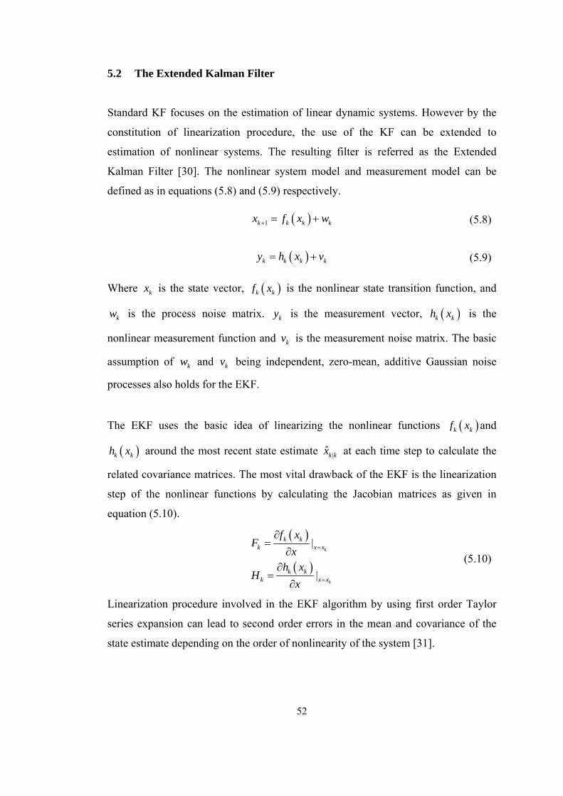
5.2 The Extended Kalman Filter

Standard KF focuses on the estimation of linear dynamic systems. However by the

constitution of linearization procedure, the use of the KF can be extended to

estimation of nonlinear systems. The resulting filter is referred as the Extended

Kalman Filter [30]. The nonlinear system model and measurement model can be

defined as in equations (5.8) and (5.9) respectively.

1k k k kx f x w (5.8)

k k ky h x vk (5.9)

Where kx is the state vector, k kf x

k

is the nonlinear state transition function, and

is the process noise matrix. kw y is the measurement vector, is the

nonlinear measurement function and is the measurement noise matrix. The basic

assumption of and being independent, zero-mean, additive Gaussian noise

processes also holds for the EKF.

k kh x

kv

kw kv

The EKF uses the basic idea of linearizing the nonlinear functions k k f x and

around the most recent state estimate k kh x |ˆk kx at each time step to calculate the

related covariance matrices. The most vital drawback of the EKF is the linearization

step of the nonlinear functions by calculating the Jacobian matrices as given in

equation (5.10).

|

|

k

k

k kk x

k kk x

f xF

xh x

Hx

x

x

(5.10)

Linearization procedure involved in the EKF algorithm by using first order Taylor

series expansion can lead to second order errors in the mean and covariance of the

state estimate depending on the order of nonlinearity of the system [31].

  52

After obtaining the linearized system and measurement models, standard KF

equations can be applied to the nonlinear system as given in Table 6 [30].

Table 6 The Extended Kalman Filter Algorithm

State Space Model

1k k k

k k k k

kx f x w

y h x v

(5.11)

Initialization Of The Filter

0 0

0 0 0 0 0

ˆ

ˆ ˆ T

x E x

P E x x x x

(5.12)

For k=0:end

Calculate Jacobians

|

|

k

k

k kk x

k kk x

f xF

xh x

Hx

x

x

(5.13)

Time Update

1| |

1| |

ˆ ˆk k k k k

Tk k k k k k k

x f x

P F P F

Q (5.14)

Kalman Gain

1

1 1| 1| 1T T

k k k k k k k k kK P H H P H R

(5.15)

Measurement Update

1| 1 1| 1 1 1|

1| 1 1 1|

ˆ ˆ ˆk k k k k k k k k

k k k k k k

x x K y h x

P I K H P

(5.16)

  53

5.3 The Unscented Kalman Filter

The state distribution is approximated as a Gaussian random variable in the EKF

implementation. Mean and covariance matrix of the state vector are propagated

through the first order linearization of the nonlinear system model. Large

linearization errors can be introduced in the mean and covariance of posterior

distribution leading to suboptimal performance and even divergence of the filter [29].

Another nonlinear estimator, Unscented Kalman Filter (UKF) approaches this

problem by carefully selecting deterministic sigma points from the Gaussian

distribution completely capturing mean vector and covariance matrix. These points

are propagated through the nonlinear function itself leading to third order errors for

any nonlinearity. Therefore, the assumption of state being Gaussian distributed holds

for both the EKF and UKF, but representation of this distribution by the help of

deterministic sigma points instead of mean and covariance matrix makes the UKF

superior in performance [32] .

The basic operation of the UKF is Unscented Transformation (UT) which is a

method of calculating the statistics of a random variable undergoing a nonlinear

transformation [30]. The sigma points are determined by the help of UT. In the

literature, there are various methods utilized for the UT. The Scaled Unscented

Transformation (SUT) is one of the sigma point selection methods which gives the

opportunity to adjust the spread of sigma points and control the higher order errors

by some design parameters [33].

The algorithm for the SUT is given in Table 7 [33]. There are three design

parameters in the given algorithm. The parameter determines the spread of sigma

points around the given state. It is usually set to a small value. The parameter is

used to incorporate the prior knowledge about the distribution of the state space

variables. The optimal value of this parameter for Gaussian distributions is asserted

as 2. The parameter , which is a secondary constant controlling higher order effects,

is usually set to 0. In the literature, there is not a compromised method for the

  54

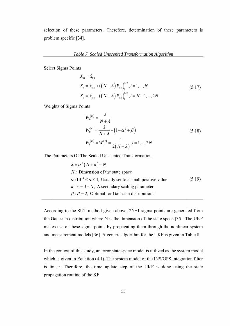
selection of these parameters. Therefore, determination of these parameters is

problem specific [34].

Table 7 Scaled Unscented Transformation Algorithm

Select Sigma Points

0 |

1/2

| |

1/2

| |

ˆ

ˆ , 1,...,

ˆ , 1,..., 2

k k

i k k k k i

i k k k k i

X x

X x N P i N

X x N P i N

N

(5.17)

Weights of Sigma Points

0

20 1

1, 1,..., 2

2

m

c

m ci i

WN

WN

W W iN

N

(5.18)

The Parameters Of The Scaled Unscented Transformation

2

4

: Dimension of the state space

:10 1, Usually set to a small positive value

: 3 , A secondary scaling parameter

: 2, Optimal for Gaussian distributions

N N

N

N

(5.19)

According to the SUT method given above, 2N+1 sigma points are generated from

the Gaussian distribution where N is the dimension of the state space [35]. The UKF

makes use of these sigma points by propagating them through the nonlinear system

and measurement models [36]. A generic algorithm for the UKF is given in Table 8.

In the context of this study, an error state space model is utilized as the system model

which is given in Equation (4.1). The system model of the INS/GPS integration filter

is linear. Therefore, the time update step of the UKF is done using the state

propagation routine of the KF.

  55

Table 8 The Unscented Kalman Filter Algorithm [32]

State Space Model

1k k k

k k k k

kx f x w

y h x v

(5.20)

Initialization of the filter

0 0

0 0 0 0 0

ˆ

ˆ ˆ T

x E x

P E x x x x

(5.21)

For k=0:end

Calculate the sigma points

ˆ ˆ ˆ k k k k k kX x x P x P (5.22)

Time Update

1|

2

1| , 1|0

2

1| , 1| 1| , 1| 1|0

ˆ

ˆˆ

ˆ ˆˆ ˆ

k k k k

Nm

k k i i k ki

N Tck k i i k k k k i k k k k k

i

X f X

x W X

P W X x X x

Q

(5.23)

Measurement Prediction

1| 1|

2

1 ,0

ˆ

ˆ

k k k k k

Nm

k i ii

Y h X

y W Y

1|k k

(5.24)

Kalman Gain

1 1

1 1

1 1 1 1

2

, 1| 1 , 1| 10

2

, 1| 1 , 1| 10

11

ˆ ˆ

ˆ ˆ ˆ

k k

k k

k k k k

N Tcy y i i k k k i k k k k

i

N Tcx y i i k k k i k k k

i

k x y y y

P W Y y Y y R

P W X x Y y

K P P

1

(5.25)

Measurement Update

1 1

1| 1 1| 1 1 1

1| 1 1 1

ˆ ˆ ˆ

k k

k k k k k k k

Tk k k y y k

x x K y y

P K P K

(5.26)

  56

5.4 The Adaptive Unscented Kalman Filter

As mentioned in Section 5.3, the underlying routine for the UKF is the UT which

determines the sigma points representing the related Gaussian distributions. Since the

SUT gives the opportunity to adjust the spread of sigma points and control the higher

order errors by some design parameters, it is selected as the UT method in the

context of this thesis.

When the effects of the SUT parameters on integrated navigation solution are

investigated, it is observed that the performance of the UKF is dependent on these

design parameters. Selection of different parameters for the same navigation scenario

results in varying navigation accuracy [37]. Also, in-flight performance of the

integration filter changes for different parts of the trajectory for a given set of SUT

parameters.

The parameter , which is usually set to a small value between 0 and 1, determines

the spread of sigma points around the given state. The parameter , whose optimal

value for Gaussian distributions is 2, is used to incorporate the prior knowledge

about the distribution of the state space variables. The parameter , which is a

secondary constant controlling higher order effects, is usually set to 0.

Among these three parameters, is the most influential one in affecting the UKF

performance. When the parameters and are set to their default values as 2 and

0, respectively, different values of changes the spread of sigma points explicitly.

In Table 9, the spread of the sigma points from the mean value of the state can be

observed as a function of the standard deviation of the state estimate . Also

related weights of the sigma points are given in the same table.

  57

Table 9 Spread of -points for different parameters Value of alpha

Distinction of -points wrt.mean

Weight

0mW

Weight

0cW

0.1 0.39 -98.99 -96.01

0.2 0.77 -24.00 -21.04

0.3 1.16 -10.11 -7.20

0.4 1.55 -5.25 -2.41

0.5 1.94 -3.00 -0.25

It can be inferred from Table 9 that, for small values of , selected sigma points are

close to the mean and they have relatively large weights. When the parameter is

raised, spread of the sigma points are extended and they move away from the mean

with reduced weights. Depending on the uncertainty of the state estimate, state

covariance matrix grows or shrinks. For large state covariance matrices, meaning

high uncertainties, a large value of the parameter results in sigma points which are

far away from the mean. It is observed from the simulations that; in the INS/GPS

integration process, such a situation may result in divergence of the UKF. But when

the uncertainties of the state estimate are low, better performance can be obtained

with larger values of the parameter . When elements of the state covariance matrix

are relatively small, a small value of the parameter results in heavily weighted

sigma points which are very close to the mean. This situation resembles to the EKF

which uses just the mean value of the state in order to represent the state estimate.

Proceeding from this point of view, selection of a common value for the parameter

is not a reasonable choice for the systems whose uncertainty may change

drastically in time which is the case for INS/GPS integrated systems. Since GPS is

vulnerable to jamming and signal blockage, intermittence of this aiding system can

occur frequently. When the GPS aiding is obtained regularly, covariance matrices

and mean of the state estimate can be kept bounded. But when the GPS outage is

considered, accuracy of the state estimate degrades with time depending on the

duration of measurement outage. Therefore, it is proposed that, different values of

  58

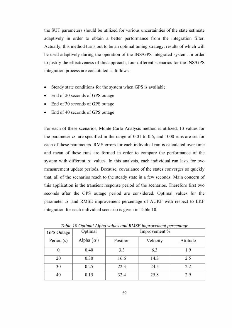
the SUT parameters should be utilized for various uncertainties of the state estimate

adaptively in order to obtain a better performance from the integration filter.

Actually, this method turns out to be an optimal tuning strategy, results of which will

be used adaptively during the operation of the INS/GPS integrated system. In order

to justify the effectiveness of this approach, four different scenarios for the INS/GPS

integration process are constituted as follows.

Steady state conditions for the system when GPS is available

End of 20 seconds of GPS outage

End of 30 seconds of GPS outage

End of 40 seconds of GPS outage

For each of these scenarios, Monte Carlo Analysis method is utilized. 13 values for

the parameter are specified in the range of 0.01 to 0.6, and 1000 runs are set for

each of these parameters. RMS errors for each individual run is calculated over time

and mean of these runs are formed in order to compare the performance of the

system with different values. In this analysis, each individual run lasts for two

measurement update periods. Because, covariance of the states converges so quickly

that, all of the scenarios reach to the steady state in a few seconds. Main concern of

this application is the transient response period of the scenarios. Therefore first two

seconds after the GPS outage period are considered. Optimal values for the

parameter and RMSE improvement percentage of AUKF with respect to EKF

integration for each individual scenario is given in Table 10.

Table 10 Optimal Alpha values and RMSE improvement percentage Improvement % GPS Outage

Period (s)

Optimal

Alpha Position Velocity Attitude

0 0.40 3.3 6.3 1.9

20 0.30 16.6 14.3 2.5

30 0.25 22.3 24.5 2.2

40 0.15 32.4 25.8 2.9

  59

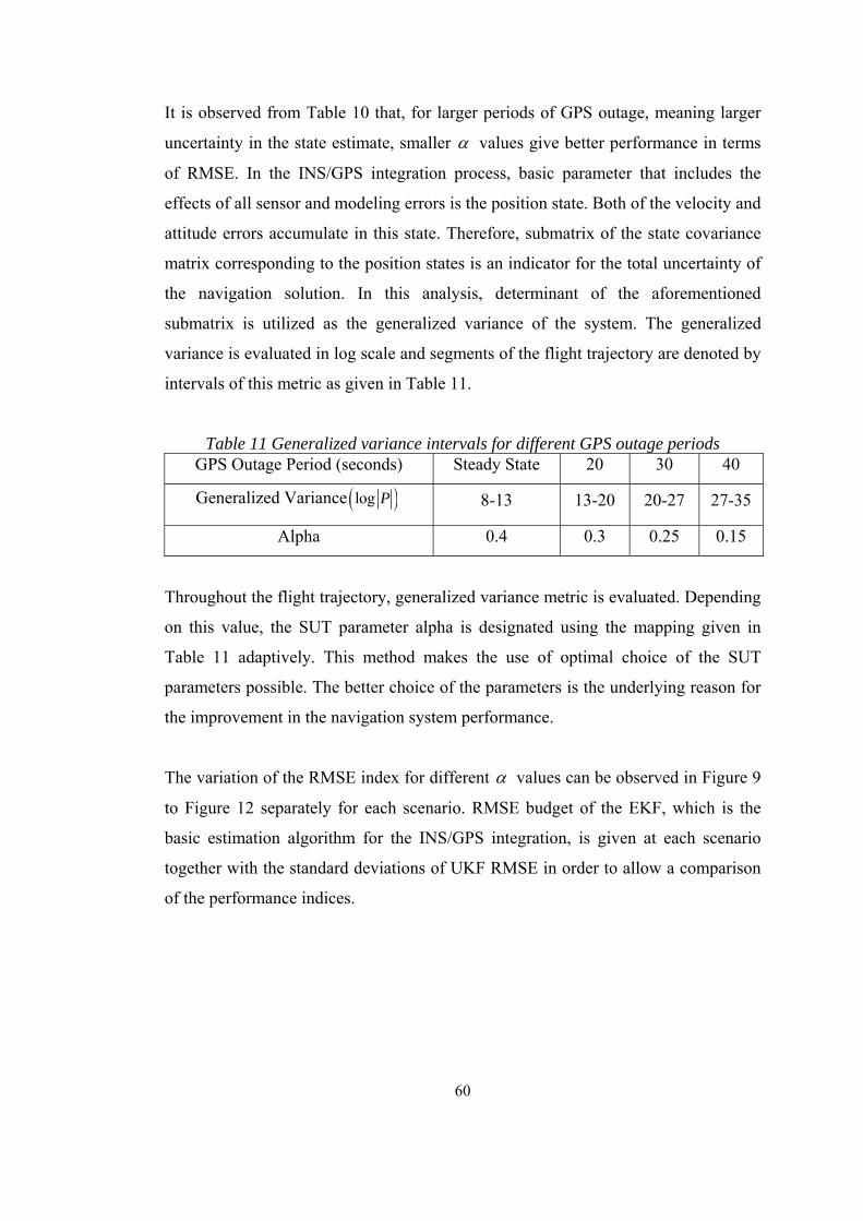
It is observed from Table 10 that, for larger periods of GPS outage, meaning larger

uncertainty in the state estimate, smaller values give better performance in terms

of RMSE. In the INS/GPS integration process, basic parameter that includes the

effects of all sensor and modeling errors is the position state. Both of the velocity and

attitude errors accumulate in this state. Therefore, submatrix of the state covariance

matrix corresponding to the position states is an indicator for the total uncertainty of

the navigation solution. In this analysis, determinant of the aforementioned

submatrix is utilized as the generalized variance of the system. The generalized

variance is evaluated in log scale and segments of the flight trajectory are denoted by

intervals of this metric as given in Table 11.

Table 11 Generalized variance intervals for different GPS outage periods GPS Outage Period (seconds) Steady State 20 30 40

Generalized Variance log P 8-13 13-20 20-27 27-35

Alpha 0.4 0.3 0.25 0.15

Throughout the flight trajectory, generalized variance metric is evaluated. Depending

on this value, the SUT parameter alpha is designated using the mapping given in

Table 11 adaptively. This method makes the use of optimal choice of the SUT

parameters possible. The better choice of the parameters is the underlying reason for

the improvement in the navigation system performance.

The variation of the RMSE index for different values can be observed in Figure 9

to Figure 12 separately for each scenario. RMSE budget of the EKF, which is the

basic estimation algorithm for the INS/GPS integration, is given at each scenario

together with the standard deviations of UKF RMSE in order to allow a comparison

of the performance indices.

  60

0 0.1 0.2 0.3 0.4 0.5 0.6 0.75.45.65.8

66.26.4

Position RMSE Mean & Mean 1

Po

s. R

MS

E (

m)

Alpha

EKFUKFMean1

0 0.1 0.2 0.3 0.4 0.5 0.6 0.70.55

0.60.65

0.70.75

0.80.85

0.9Velocity RMSE Mean & Mean 1

Ve

l. R

MS

E(m

/s)

Alpha

EKFUKFMean1

0 0.1 0.2 0.3 0.4 0.5 0.6 0.70.330.340.350.360.370.380.39

0.4Attitude RMSE Mean & Mean 1

Alpha

Att.

RM

SE

(de

g)

UKFEKFMean1

Figure 9 RMSE variations over alpha values for Steady state conditions

0 0.1 0.2 0.3 0.4 0.5 0.6 0.70

20406080

100Position RMSE Mean & Mean 1

Po

s. R

MS

E (

m)

Alpha

EKFUKFMean1

0 0.1 0.2 0.3 0.4 0.5 0.6 0.70.20.40.60.8

11.2

Velocity RMSE Mean & Mean 1

Ve

l. R

MS

E(m

/s)

Alpha

EKFUKFMean1

0 0.1 0.2 0.3 0.4 0.5 0.6 0.70.430.440.450.460.470.480.49

0.5Attitude RMSE Mean & Mean 1

Alpha

Att.

RM

SE

(de

g)

UKFEKFMean1

Figure 10 RMSE variations over alpha values for 20 seconds GPS Outage

  61

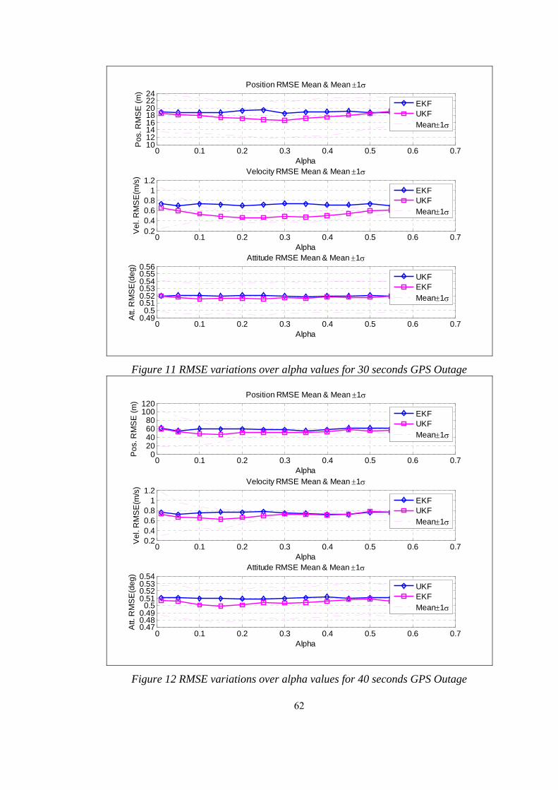
0 0.1 0.2 0.3 0.4 0.5 0.6 0.71012141618202224

Position RMSE Mean & Mean 1

Po

s. R

MS

E (

m)

Alpha

EKFUKFMean1

0 0.1 0.2 0.3 0.4 0.5 0.6 0.70.20.40.60.8

11.2

Velocity RMSE Mean & Mean 1

Ve

l. R

MS

E(m

/s)

Alpha

EKFUKFMean1

0 0.1 0.2 0.3 0.4 0.5 0.6 0.70.49

0.50.510.520.530.540.550.56

Attitude RMSE Mean & Mean 1

Alpha

Att.

RM

SE

(de

g)

UKFEKFMean1

Figure 11 RMSE variations over alpha values for 30 seconds GPS Outage

0 0.1 0.2 0.3 0.4 0.5 0.6 0.70

20406080

100120

Position RMSE Mean & Mean 1

Po

s. R

MS

E (

m)

Alpha

EKFUKFMean1

0 0.1 0.2 0.3 0.4 0.5 0.6 0.70.20.40.60.8

11.2

Velocity RMSE Mean & Mean 1

Ve

l. R

MS

E(m

/s)

Alpha

EKFUKFMean1

0 0.1 0.2 0.3 0.4 0.5 0.6 0.70.470.480.49

0.50.510.520.530.54

Attitude RMSE Mean & Mean 1

Alpha

Att.

RM

SE

(de

g)

UKFEKFMean1

Figure 12 RMSE variations over alpha values for 40 seconds GPS Outage

  62

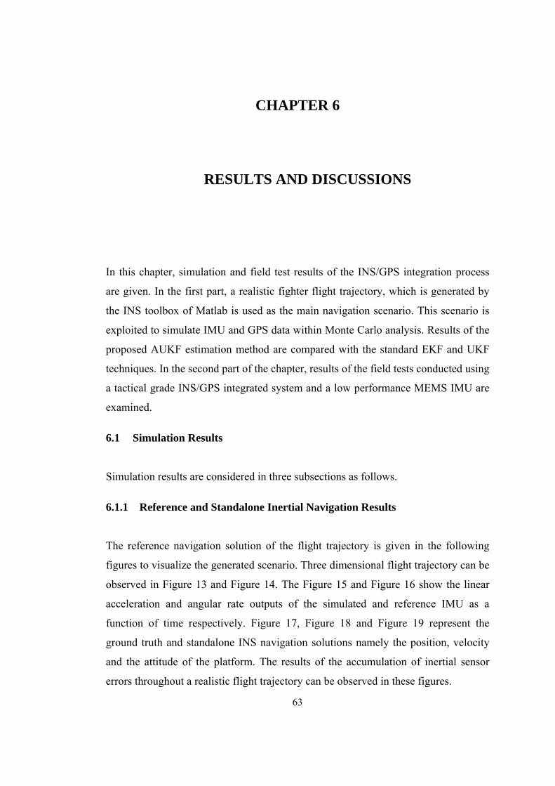
  63

CHAPTER 6

6 RESULTS AND DISCUSSIONS

In this chapter, simulation and field test results of the INS/GPS integration process

are given. In the first part, a realistic fighter flight trajectory, which is generated by

the INS toolbox of Matlab is used as the main navigation scenario. This scenario is

exploited to simulate IMU and GPS data within Monte Carlo analysis. Results of the

proposed AUKF estimation method are compared with the standard EKF and UKF

techniques. In the second part of the chapter, results of the field tests conducted using

a tactical grade INS/GPS integrated system and a low performance MEMS IMU are

examined.

6.1 Simulation Results

Simulation results are considered in three subsections as follows.

6.1.1 Reference and Standalone Inertial Navigation Results

The reference navigation solution of the flight trajectory is given in the following

figures to visualize the generated scenario. Three dimensional flight trajectory can be

observed in Figure 13 and Figure 14. The Figure 15 and Figure 16 show the linear

acceleration and angular rate outputs of the simulated and reference IMU as a

function of time respectively. Figure 17, Figure 18 and Figure 19 represent the

ground truth and standalone INS navigation solutions namely the position, velocity

and the attitude of the platform. The results of the accumulation of inertial sensor

errors throughout a realistic flight trajectory can be observed in these figures.

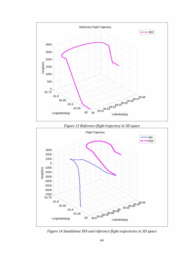
3939.01

39.0239.03

39.0439.05

39.0639.07

39.08

-82

-81.95

-81.9

-81.85

-81.8

-81.750

500

1000

1500

2000

2500

3000

Latitude(deg)

Reference Flight Trajectory

Longitude(deg)

He

igh

t(m

)

REF

Figure 13 Reference flight trajectory in 3D space

38.938.92

38.9438.96

38.9839

39.0239.04

39.0639.08

-82

-81.95

-81.9

-81.85

-81.8

-81.75-7000

-6000

-5000

-4000

-3000

-2000

-1000

0

1000

2000

3000

Latitude(deg)

Flight Trajectory

Longitude(deg)

He

igh

t(m

)

INSREF

Figure 14 Standalone INS and reference flight trajectories in 3D space

  64

0 50 100 150 200 250-10

-505

1015

X-axis Acceleration

Time(s)

ax(

m/s

2)

INSREF

0 50 100 150 200 250-3-2-1012

Y-axis Acceleration

Time(s)

ay(

m/s

2)

INSREF

0 50 100 150 200 250-150-100

-500

50100

Z-axis Acceleration

Time(s)

az(

m/s

2)

INSREF

Figure 15 Simulated acceleration output of the IMU

0 50 100 150 200 250-3-2-10123

X-axis Angular Rate

Time(s)

p(d

eg

/s)

INSREF

0 50 100 150 200 250-1.5

-1-0.5

00.5

11.5

Y-axis Angular Rate

Time(s)

q(d

eg

/s)

INSREF

0 50 100 150 200 250-0.2

-0.15-0.1

-0.050

0.050.1

0.15Z-axis Angular Rate

Time(s)

r(d

eg

/s)

INSREF

Figure 16 Simulated angular rate output of the IMU

  65

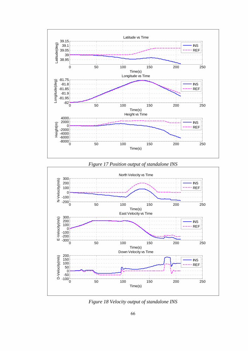
0 50 100 150 200 250

38.9539

39.0539.1

39.15Latitude vs Time

Time(s)

La

titu

de

(de

g)

INSREF

0 50 100 150 200 250-82

-81.95-81.9

-81.85-81.8

-81.75Longitude vs Time

Time(s)

Lo

ng

itud

e(d

eg

)

INSREF

0 50 100 150 200 250-8000-6000-4000-2000

020004000

Height vs Time

Time(s)

He

igh

t(m

)

INSREF

Figure 17 Position output of standalone INS

0 50 100 150 200 250-200-100

0100200300

North Velocity vs Time

Time(s)

N-V

elo

city

(m/s

)

INSREF

0 50 100 150 200 250-300-200-100

0100200300

East Velocity vs Time

Time(s)

E-V

elo

city

(m/s

)

INSREF

0 50 100 150 200 250-100

-500

50100150200

Down Velocity vs Time

Time(s)

D-V

elo

city

(m/s

)

INSREF

Figure 18 Velocity output of standalone INS

  66

0 50 100 150 200 250-60-50-40-30-20-10

010

Phi Angle vs Time

Time(s)

Ph

i(d

eg

)

INSREF

0 50 100 150 200 250-40-30-20-10

0102030

Theta Angle vs Time

Time(s)

Th

eta

(de

g)

INSREF

0 50 100 150 200 250-100

-50

0

50

100Psi Angle vs Time

Time(s)

Psi

(de

g)

INSREF

Figure 19 Attitude output of standalone INS

It is clear from Figure 14 that a low cost MEMS IMU can not be used as a sole

navigation system after a few minutes from the take off. Accumulation of large

errors present in the outputs of the low performance inertial sensors result in large-

scaled navigation errors which can not be tolerated for most of the moving platforms.

This result makes integration of two complementary systems, namely INS and GPS

essential.

6.1.2 Standard EKF and UKF Results

Low cost and low performance MEMS IMU is integrated with the GPS in a tightly-

coupled architecture using the standard EKF and UKF algorithms. Identical system

and measurement models are utilized in both of the filters. The same initial state

covariance, process noise and measurement noise matrices are used in the estimation

algorithms for a meaningful comparison of the performances.

  67

  68

As mentioned in section 4.6, the nonlinearity of the INS/GPS integrated system

stems from the utilization of the nonlinear measurement model. In the presence of

the regular measurements, the estimation error of the navigation solution is kept

bounded. Therefore, the nonlinearity in the measurements can easily be handled by

the EKF.

When large initial state errors and covariances are considered, the first order

approximation of the EKF becomes insufficient to cope with the nonlinearity. These

situations may result in even divergence of the filter. Since GPS is vulnerable to

jamming and signal blockage, outage of this aiding system should be considered

carefully. Intermittence of the GPS measurements results in large initial state errors

and large initial state covariances for the estimation algorithms depending on the

period of standalone practice of the INS. In the course of the analysis, three GPS

outage periods are modeled to create a compelling scenario for the estimation

algorithms. Hence the actual performance of the EKF and the UKF are compared in a

more compelling and realistic case. Simulated GPS outage periods are summarized

in the following table.

Table 12 GPS outage periods in the flight trajectory GPS Availability OFF ON OFF ON OFF ON

Time Period (s) 0-20 20-60 60-90 90-130 130-170 170-210

In Figure 20 to Figure 29, estimation errors for the curvilinear position, the velocity,

the attitude and the sensor biases for a single scenario are presented together with the

standard deviations of the two estimation algorithms consecutively. In Figure 30, the

Root Mean Square Error values of the two filters throughout the trajectory are given

in order to compare the performances.

0 50 100 150 200 250-3-2-10123

x 10-3 Latitude Error & 1

La

t-E

rro

r(d

eg

)

Time(s)

Error

1

0 50 100 150 200 250-4-20246

x 10-3 Longitude Error & 1

Lo

n-E

rro

r(d

eg

)

Time(s)

Error

1

0 50 100 150 200 250-400

-200

0

200

400Height Error & 1

H-E

rro

r(m

)

Time(s)

Error

1

Figure 20 EKF Position estimation error and 1 error bound

0 50 100 150 200 250-20

-10

0

10

20North Velocity Error & 1

N-V

el-

Err

or(

m/s

)

Time(s)

Error

1

0 50 100 150 200 250-20

-10

0

10

20East Velocity Error & 1

E-V

el-

Err

or(

m/s

)

Time(s)

Error

1

0 50 100 150 200 250-20

-10

0

10

20Down Velocity Error & 1

D-V

el-

Err

or(

m/s

)

Time(s)

Error

1

Figure 21 EKF Velocity estimation error and 1 error bound

  69

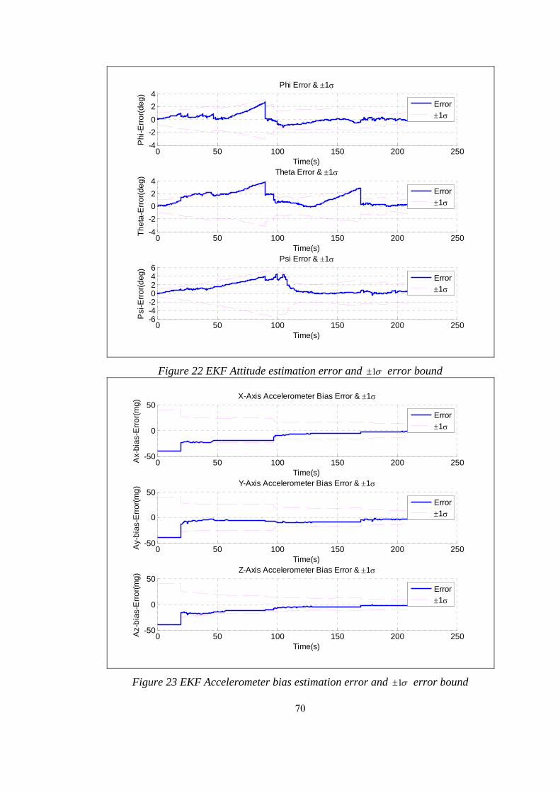
0 50 100 150 200 250-4

-2

0

2

4Phi Error & 1

Ph

i-E

rro

r(d

eg

)

Time(s)

Error

1

0 50 100 150 200 250-4

-2

0

2

4Theta Error & 1

Th

eta

-Err

or(

de

g)

Time(s)

Error

1

0 50 100 150 200 250-6-4-20246

Psi Error & 1

Psi

-Err

or(

de

g)

Time(s)

Error

1

Figure 22 EKF Attitude estimation error and 1 error bound

0 50 100 150 200 250-50

0

50X-Axis Accelerometer Bias Error & 1

Ax-

bia

s-E

rro

r(m

g)

Time(s)

Error

1

0 50 100 150 200 250-50

0

50Y-Axis Accelerometer Bias Error & 1

Ay-

bia

s-E

rro

r(m

g)

Time(s)

Error

1

0 50 100 150 200 250-50

0

50Z-Axis Accelerometer Bias Error & 1

Az-

bia

s-E

rro

r(m

g)

Time(s)

Error

1

Figure 23 EKF Accelerometer bias estimation error and 1 error bound

  70

0 50 100 150 200 250-300-200-100

0100200300

X-Axis Gyroscope Bias Error & 1

Gx-

bia

s-E

rro

r(d

eg

/h)

Time(s)

Error

1

0 50 100 150 200 250-300-200-100

0100200300

Y-Axis Gyroscope Bias Error & 1

Gy-

bia

s-E

rro

r(d

eg

/h)

Time(s)

Error

1

0 50 100 150 200 250-300-200-100

0100200300

Z-Axis Gyroscope Bias Error & 1

Gz-

bia

s-E

rro

r(d

eg

/h)

Time(s)

Error

1

Figure 24 EKF Accelerometer bias estimation error and 1 error bound

0 50 100 150 200 250-3-2-10123

x 10-3 Latitude Error & 1

La

t-E

rro

r(d

eg

)

Time(s)

Error

1

0 50 100 150 200 250-4-20246

x 10-3 Longitude Error & 1

Lo

n-E

rro

r(d

eg

)

Time(s)

Error

1

0 50 100 150 200 250-400

-200

0

200

400Height Error & 1

H-E

rro

r(m

)

Time(s)

Error

1

Figure 25 UKF Position estimation error and 1 error bound

  71

0 50 100 150 200 250-20

0

20North Velocity Error & 1

N-V

el-

Err

or(

m/s

)

Time(s)

Error

1

0 50 100 150 200 250-20

0

20East Velocity Error & 1

E-V

el-

Err

or(

m/s

)

Time(s)

Error

1

0 50 100 150 200 250-20

0

20Down Velocity Error & 1

D-V

el-

Err

or(

m/s

)

Time(s)

Error

1

Figure 26 UKF Velocity estimation error and 1 error bound

0 50 100 150 200 250-4

-2

0

2

4Phi Error & 1

Ph

i-E

rro

r(d

eg

)

Time(s)

Error

1

0 50 100 150 200 250-4

-2

0

2

4Theta Error & 1

Th

eta

-Err

or(

de

g)

Time(s)

Error

1

0 50 100 150 200 250-6-4-20246

Psi Error & 1

Psi

-Err

or(

de

g)

Time(s)

Error

1

Figure 27 UKF Attitude estimation error and 1 error bound

  72

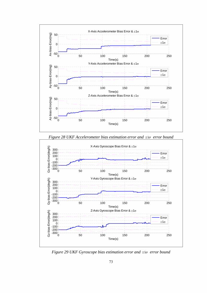
0 50 100 150 200 250-50

0

50X-Axis Accelerometer Bias Error & 1

Ax-

bia

s-E

rro

r(m

g)

Time(s)

Error

1

0 50 100 150 200 250-50

0

50Y-Axis Accelerometer Bias Error & 1

Ay-

bia

s-E

rro

r(m

g)

Time(s)

Error

1

0 50 100 150 200 250-50

0

50Z-Axis Accelerometer Bias Error & 1

Az-

bia

s-E

rro

r(m

g)

Time(s)

Error

1

Figure 28 UKF Accelerometer bias estimation error and 1 error bound

0 50 100 150 200 250-300-200-100

0100200300

X-Axis Gyroscope Bias Error & 1

Gx-

bia

s-E

rro

r(d

eg

/h)

Time(s)

Error

1

0 50 100 150 200 250-300-200-100

0100200300

Y-Axis Gyroscope Bias Error & 1

Gy-

bia

s-E

rro

r(d

eg

/h)

Time(s)

Error

1

0 50 100 150 200 250-300-200-100

0100200300

Z-Axis Gyroscope Bias Error & 1

Gz-

bia

s-E

rro

r(d

eg

/h)

Time(s)

Error

1

Figure 29 UKF Gyroscope bias estimation error and 1 error bound

  73

Performance of the EKF and the UKF algorithms are compared in terms of the Root

Mean Square Error (RMSE) metrics which are obtained using the results of Monte

Carlo Simulations in which the stochastic IMU and GPS error parameters are set

randomly. RMSE of the results are calculated using the Equation (6.1).

2 2

1 1

1 1N KREF REF REF

k k k k k kn k

RMSE x x y y z zN K

2

(6.1)

where is the number of Monte Carlo runs and is the number of time steps in

the scenario.

N K

, ,REF REF REFk k kx y z are the error-free reference data and , ,k k kx y z are

the state estimates of the filter at time step k.

The RMSE results for EKF and UKF are obtained using 1000 Monte Carlo runs.

Variation of the two estimators’ RMSE performance in time is given in Figure 30.

0 50 100 150 200 2500

100200300400500

Position RMSE vs Time (EKF:108.3414 / UKF:107.2512)

Time(s)

Po

s. R

mse

(m)

EKFUKF

0 50 100 150 200 25005

10152025

Velocity RMSE vs Time (EKF:7.4364 / UKF:7.3852)

Time(s)

Ve

l. R

mse

(m/s

)

EKFUKF

0 50 100 150 200 2500123456

Attitude RMSE vs Time (EKF:2.3668 / UKF:2.2982)

Time(s)

Att.

Rm

se(d

eg

)

EKFUKF

Figure 30 Comparison of EKF and UKF RMSE metrics  

  74

A close look at the Figure 30 shows that the standard UKF slightly improves the

performance of the EKF. For comparison, RMSE’s of the estimated navigation

solutions are given below in Table 13.

Table 13 RMSE Performance comparison of EKF and UKF RMSE POSITION VELOCITY ATTITUDE

EKF 108.3414 7.4364 2.3668

UKF 107.2512 7.3852 2.2982

Improvement 1.01 % 0.689 % 2.89 %

However, when different segments of the flight trajectory are considered separately,

UKF does not have superior performance at all times. This case can be observed by

simply zooming in to Figure 30. While the position RMSE of the UKF is barely

larger than that of the EKF at the end of 20 seconds GPS outage, UKF has better

performance than the EKF at the end of 30 and 40 seconds of GPS outage periods as

seen in Figure 31.

20 20.5 21 21.5 22 22.5 23 23.5 24 24.5 250

5

10

15

20

Time(s)

Po

s. R

mse

(m)

Position RMSE vs Time (Time Segment: 20-25)

EKFUKF

90 90.5 91 91.5 92 92.5 93 93.5 94 94.5 950

1020304050

Time(s)

Po

s. R

mse

(m)

Position RMSE vs Time (Time Segment: 90-95)

EKFUKF

170 170.5 171 171.5 172 172.5 173 173.5 174 174.5 1750

10203040506070

Time(s)

Po

s. R

mse

(m)

Position RMSE vs Time (Time Segment: 170-175)

EKFUKF

Figure 31 Position RMSE values of EKF&UKF (Zoomed version of Figure 30)

  75

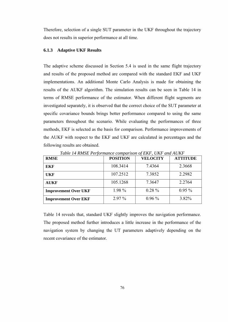
  76

Therefore, selection of a single SUT parameter in the UKF throughout the trajectory

does not results in superior performance at all time.

6.1.3 Adaptive UKF Results

The adaptive scheme discussed in Section 5.4 is used in the same flight trajectory

and results of the proposed method are compared with the standard EKF and UKF

implementations. An additional Monte Carlo Analysis is made for obtaining the

results of the AUKF algorithm. The simulation results can be seen in Table 14 in

terms of RMSE performance of the estimator. When different flight segments are

investigated separately, it is observed that the correct choice of the SUT parameter at

specific covariance bounds brings better performance compared to using the same

parameters throughout the scenario. While evaluating the performances of three

methods, EKF is selected as the basis for comparison. Performance improvements of

the AUKF with respect to the EKF and UKF are calculated in percentages and the

following results are obtained.

Table 14 RMSE Performance comparison of EKF, UKF and AUKF RMSE POSITION VELOCITY ATTITUDE

EKF 108.3414 7.4364 2.3668

UKF 107.2512 7.3852 2.2982

AUKF 105.1268 7.3647 2.2764

Improvement Over UKF 1.98 % 0.28 % 0.95 %

Improvement Over EKF 2.97 % 0.96 % 3.82%

Table 14 reveals that, standard UKF slightly improves the navigation performance.

The proposed method further introduces a little increase in the performance of the

navigation system by changing the UT parameters adaptively depending on the

recent covariance of the estimator.

6.2 Field Test Results

A field test is conducted using a tactical grade INS/GPS integrated system as the

reference and a stabilization grade low performance IMU as the unit under test.

These two systems can be seen in Figure 32.

a. b.

Figure 32 Navigation Systems: a. FOG INS/GPS- CNS5000, b. MEMS IMU-MTi

CNS5000 is a high performance INS/GPS integrated navigation system of KVH

Industries Inc. which uses a tactical grade FOG IMU. MTi is a low cost - low

performance MEMS IMU of Xsens Technologies Inc.

In the test setup, both of the navigation systems are located in a passenger car side by

side and GPS antenna of the reference system is attached on the top of the car. An

overview of the test set-up for the reference system is given in the following figure.

The utilized MEMS IMU is directly connected to the USB port of the test-PC.

  77

Figure 33 Test set-up for the reference system (Figure is adapted from [38])

In the rest of the thesis, measurements and navigation results of the high performance

INS/GPS integrated system CNS5000 is referred to as reference (REF in short).

Outputs of the low performance IMU MTi is referred to as MEMS.

In Figure 34 and Figure 35, linear acceleration and angular rate measurements of the

two navigation units are given, respectively.

  78

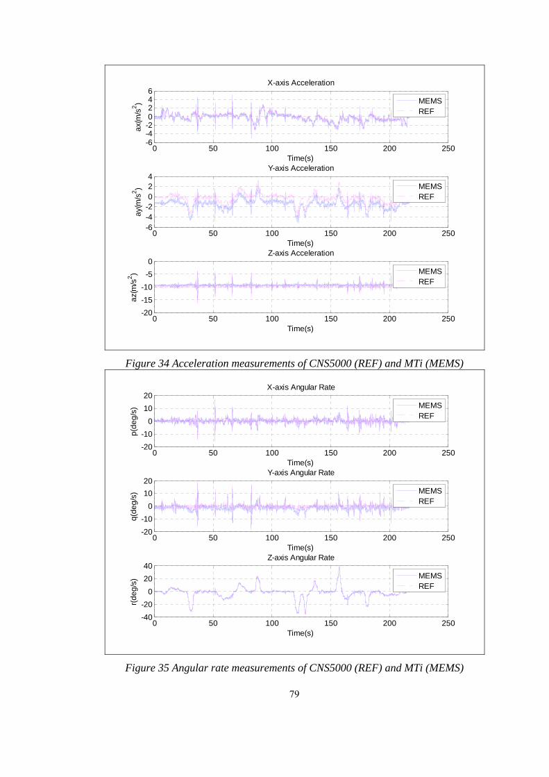
0 50 100 150 200 250-6-4-20246

X-axis Acceleration

Time(s)

ax(

m/s

2)

MEMSREF

0 50 100 150 200 250-6-4-2024

Y-axis Acceleration

Time(s)

ay(

m/s

2)

MEMSREF

0 50 100 150 200 250-20

-15

-10

-5

0Z-axis Acceleration

Time(s)

az(

m/s

2)

MEMSREF

Figure 34 Acceleration measurements of CNS5000 (REF) and MTi (MEMS)

0 50 100 150 200 250-20

-10

0

10

20X-axis Angular Rate

Time(s)

p(d

eg

/s)

MEMSREF

0 50 100 150 200 250-20

-10

0

10

20Y-axis Angular Rate

Time(s)

q(d

eg

/s)

MEMSREF

0 50 100 150 200 250-40

-20

0

20

40Z-axis Angular Rate

Time(s)

r(d

eg

/s)

MEMSREF

Figure 35 Angular rate measurements of CNS5000 (REF) and MTi (MEMS)

  79

6.2.1 Test Results without GPS Outages

Navigation results namely position, velocity and attitude of the test vehicle obtained

by AUKF algorithm are given together with the reference system outputs in Figure

36 toFigure 40.

39.98639.9865

39.98739.9875

39.98839.9885

39.98939.9895

39.9939.9905

39.991

33.10233.1025

33.10333.1035

33.10433.1045

33.10533.1055

33.10633.1065

33.1071160

1165

1170

1175

1180

1185

1190

1195

1200

Latitude(deg)

Flight Trajectory

Longitude(deg)

Hei

ght(

m)

AUKF

REF

Figure 36 3D Flight trajectory computed by the reference system and AUKF

  80

39.986 39.987 39.988 39.989 39.99 39.991 39.99233.102

33.1025

33.103

33.1035

33.104

33.1045

33.105

33.1055

33.106

33.1065

33.107 Flight Trajectory

Latitude(deg)

Lo

ng

itud

e(d

eg

)

AUKFREF

Figure 37 Horizontal position computed by the reference system and AUKF

0 50 100 150 200 25039.98639.98739.98839.989

39.9939.99139.992

Latitude vs Time

Time(s)

La

titu

de

(de

g)

AUKFREF

0 50 100 150 200 25033.10233.10333.10433.10533.10633.10733.108

Longitude vs Time

Time(s)

Lo

ng

itud

e(d

eg

)

AUKFREF

0 50 100 150 200 250116011701180119012001210

Height vs Time

Time(s)

He

igh

t(m

)

AUKFREF

Figure 38 Position output computed by the reference system and AUKF

  81

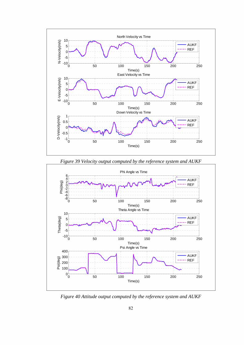
0 50 100 150 200 250-10

-5

0

5

10North Velocity vs Time

Time(s)

N-V

elo

city

(m/s

)

AUKFREF

0 50 100 150 200 250-10

-5

0

5

10East Velocity vs Time

Time(s)

E-V

elo

city

(m/s

)

AUKFREF

0 50 100 150 200 250-1

-0.5

0

0.5

1Down Velocity vs Time

Time(s)

D-V

elo

city

(m/s

)

AUKFREF

Figure 39 Velocity output computed by the reference system and AUKF

0 50 100 150 200 250-8-6-4-20246

Phi Angle vs Time

Time(s)

Ph

i(d

eg

)

AUKFREF

0 50 100 150 200 250-10

-5

0

5

10Theta Angle vs Time

Time(s)

Th

eta

(de

g)

AUKFREF

0 50 100 150 200 2500

100

200

300

400Psi Angle vs Time

Time(s)

Psi

(de

g)

AUKFREF

Figure 40 Attitude output computed by the reference system and AUKF

  82

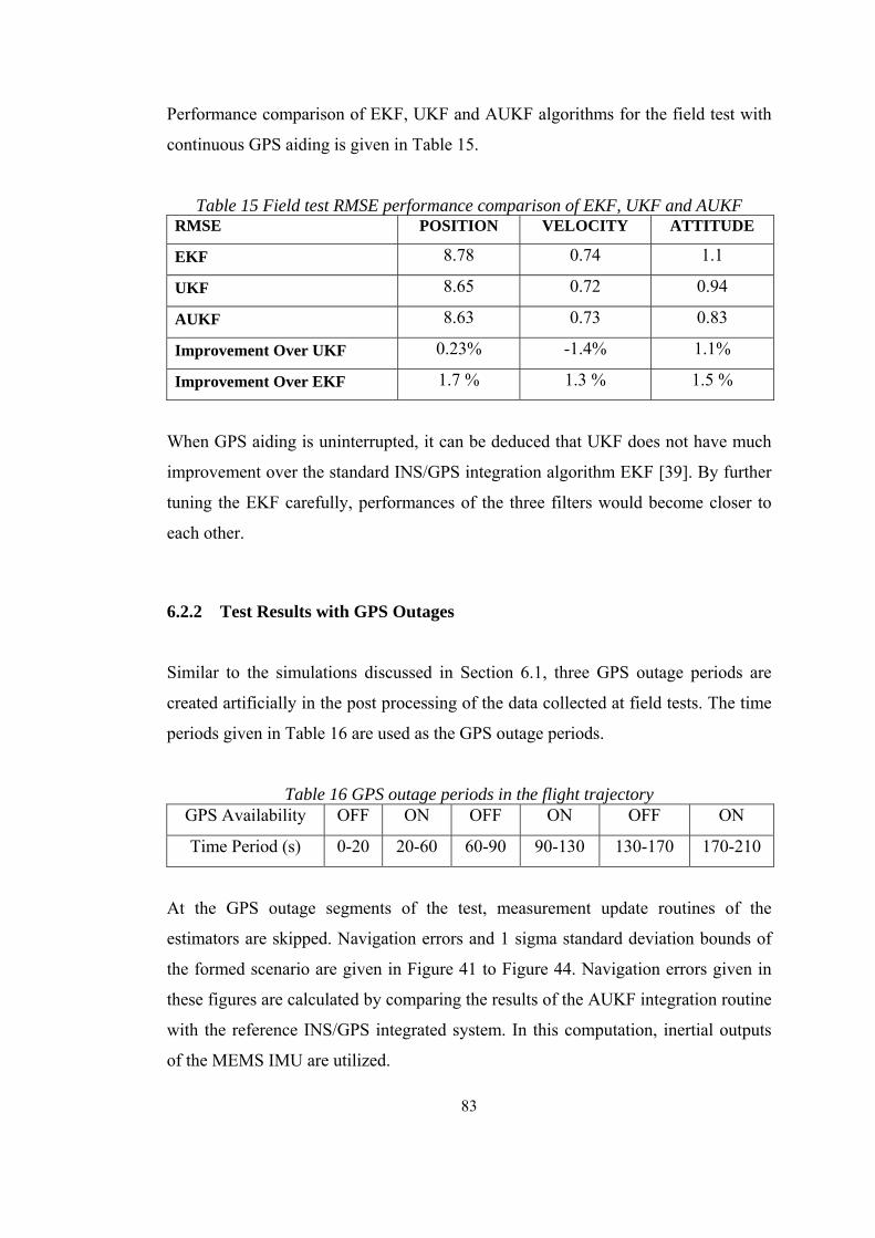
  83

Performance comparison of EKF, UKF and AUKF algorithms for the field test with

continuous GPS aiding is given in Table 15.

Table 15 Field test RMSE performance comparison of EKF, UKF and AUKF RMSE POSITION VELOCITY ATTITUDE

EKF 8.78 0.74 1.1

UKF 8.65 0.72 0.94

AUKF 8.63 0.73 0.83

Improvement Over UKF 0.23% -1.4% 1.1%

Improvement Over EKF 1.7 % 1.3 % 1.5 %

When GPS aiding is uninterrupted, it can be deduced that UKF does not have much

improvement over the standard INS/GPS integration algorithm EKF [39]. By further

tuning the EKF carefully, performances of the three filters would become closer to

each other.

6.2.2 Test Results with GPS Outages

Similar to the simulations discussed in Section 6.1, three GPS outage periods are

created artificially in the post processing of the data collected at field tests. The time

periods given in Table 16 are used as the GPS outage periods.

Table 16 GPS outage periods in the flight trajectory GPS Availability OFF ON OFF ON OFF ON

Time Period (s) 0-20 20-60 60-90 90-130 130-170 170-210

At the GPS outage segments of the test, measurement update routines of the

estimators are skipped. Navigation errors and 1 sigma standard deviation bounds of

the formed scenario are given in Figure 41 to Figure 44. Navigation errors given in

these figures are calculated by comparing the results of the AUKF integration routine

with the reference INS/GPS integrated system. In this computation, inertial outputs

of the MEMS IMU are utilized.

0 50 100 150 200 250-3-2-10123

x 10-3 Latitude Error & 1

La

t-E

rro

r(d

eg

)

Time(s)

Error

1

0 50 100 150 200 250-6-4-2024

x 10-3 Longitude Error & 1

Lo

n-E

rro

r(d

eg

)

Time(s)

Error

1

0 50 100 150 200 250-400-300-200-100

0100200300

Height Error & 1

H-E

rro

r(m

)

Time(s)

Error

1

Figure 41 AUKF Position estimation error and 1 error bound

0 50 100 150 200 250-15-10

-505

1015

North Velocity Error & 1

N-V

el-

Err

or(

m/s

)

Time(s)

Error

1

0 50 100 150 200 250-20-15-10

-505

1015

East Velocity Error & 1

E-V

el-

Err

or(

m/s

)

Time(s)

Error

1

0 50 100 150 200 250-15-10

-505

101520

Down Velocity Error & 1

D-V

el-

Err

or(

m/s

)

Time(s)

Error

1

Figure 42 AUKF Position estimation error and 1 error bound

  84

0 50 100 150 200 250-3-2-101234

Phi Error & 1

Ph

i-E

rro

r(d

eg

)

Time(s)

Error

1

0 50 100 150 200 250-4-3-2-10123

Theta Error & 1

Th

eta

-Err

or(

de

g)

Time(s)

Error

1

0 50 100 150 200 250-10

-5

0

5

10Psi Error & 1

Psi

-Err

or(

de

g)

Time(s)

Error

1

Figure 43 AUKF Position estimation error and 1 error bound

0 50 100 150 200 2500

100200300400500600700

Position RMSE vs Time (EKF:170.0148 / AUKF:163.2533)

Po

s. R

mse

(m)

EKFAUKF

0 50 100 150 200 25005

1015202530

Velocity RMSE vs Time (EKF:7.7596 / AUKF:7.4821)

Ve

l. R

mse

(m/s

)

EKFAUKF

0 50 100 150 200 2500

1

2

3

4Attitude RMSE vs Time (EKF:2.1126 / AUKF:1.8078)

Time(s)

Att.

Rm

se(d

eg

)

EKFAUKF

Figure 44 AUKF Position estimation error and 1 error bound

  85

  86

A summary of the results obtained from the collected data is given in Table 17.

Table 17 Field test RMSE performance comparison of EKF, UKF and AUKF RMSE POSITION VELOCITY ATTITUDE

EKF 170.0148 7.7596 2.1126

UKF 168.2164 7.7612 2.0127

AUKF 163.2533 7.4821 1.8078

Improvement Over UKF 2.95 % 3.60 % 11.33 %

Improvement Over EKF 3.98% 3.58% 14.43%

It is observed that, the AUKF algorithm improves the navigation performance by an

amount of about 4 percent in the position, 3.5 percent in the velocity and 15 percent

in the attitude when compared to the EKF within a scenario including various GPS

outages. Due to the selection of the optimal SUT parameters, results of the UKF

algorithm are further increased by a small amount.

  87

CHAPTER 7

7 CONCLUSIONS

In this thesis, the INS/GPS integration is examined and three estimation techniques

have been utilized in the context of the study. As a standard and most widely used

algorithm, the Extended Kalman Filter is used to solve the regarding estimation

problem. In order to improve the performance of the standard INS/GPS integration

routine, Unscented Kalman Filter and Adaptive Unscented Kalman Filter

implementations are utilized. Designed algorithms are verified and validated as a part

of a realistic simulation within the Monte Carlo Analysis. In addition to the

simulations, the results are proven with field tests conducted.

Initially, the fundamental information about the inertial navigation systems is

presented. The Earth and the gravity models, the error models of the inertial

measurement unit, the inertial navigation mechanization equations, and the linear

error model of the INS, which is the system model of the designed estimators, are

discussed in detail.

After providing the fundamental characteristics of the Global Positioning System,

related measurement model and the measurement errors are discussed. A nonlinear

measurement model is obatined. The constituted state space and the measurement

model for the INS/GPS integration process are used within the estimators which are

discussed in detail.

  88

Finally, the results obtained from the simulations and the field tests are presented and

performances of the three estimators are compared in terms of RMSE of the

navigation outputs.

It is concluded that UKF provides only a slight improvement in the navigation

performance over EKF. When the GPS aiding is obtained regularly, covariance

matrices and mean of the state estimate can be kept bounded. In this situation,

satisfactory estimation accuracy can be obtained from EKF.

When the GPS outages are considered, accuracy of the standalone navigation

deteriorates with the duration of the measurement outage periods. Large GPS outage

periods result in large initial state errors and large initial state covariance for the

estimators Due to the inaccuracy in the initialization of the estimator states at the end

of intermittence of measurements, degradation occurs in the EKF INS/GPS

integration in terms of accuracy and convergence time. The underlying reason for

this situation is the fact that the first order approximation of the EKF becomes

insufficient to cope with the growing nonlinearity [40]. By a proper selection of the

parameters of the SUT method, up to fourth order accuracy for any nonlinearity can

be obtained from the UKF [32].

One of the most important result of the simulations is that, the performance

improvement of the UKF over the EKF increases with increasing initialization errors

which means increasing nonlinearity.

When the effects of the SUT parameters on the integrated navigation solution are

investigated, it is observed that the performance of the UKF depends on these design

parameters. Selection of different parameters for the same navigation scenario results

in varying navigation accuracy. Proper designation of the SUT parameters in the

context of the AUKF further introduces little increase in the performance of the

navigation system. This method is applied by changing the SUT parameters

adaptively depending on the recent covariance of the estimator. It is found from the

simulations and the field test results that, the correct choice of the SUT parameters at

  89

specific covariance bounds brings better performance compared to using fixed

parameters throughout the scenario.

To further increase the performance of the AUKF, the number of covariance bounds

which are defined for specific a SUT parameters can be increased as a feature work.

By increasing the test points for finding optimal SUT parameters, these parameters

can be selected more accurately.

In the proposed adaptive method, adaptiveness of the selection of the SUT

parameters depends on the determinant of the covariance matrix of the position

states. Further analysis can be done by using different metrics, such as the trace of

the covariance matrix or the filter innovations.

Finally, by making a detailed stochastic observability analysis, further insight can be

gained about the AUKF. The effects of the navigation scenario on the performance

of the integration algorithm can be observed by considering the observabilities of the

individual estimation filter states.

  90

REFERENCES

[1] Hofmann Wellenhof, Klaus Legat, Manferd Wieser, Navigation: Principles

of Positioning and Guidance, Springer-Verlag Wien New York, 2003

[2] Averil B. Chatfield, Fundamentals of High Accuracy Inertial Navigation,

American Institute of Aeronautics and Astronautics, Inc., 1997

[3] Mohinder S. Grewal, L.R. Weill, A.P. Andrews, Global Positioning

Systems, Inertial Navigation & Integration, John Wiley and Sons, New

York, 2007

[4] Daniel J. Biezad, Integrated Navigation and Guidance Systems, American

Institute of Aeronautics and Astronautics, Inc., 1999

[5] Christopher Jekeli, Integrated Navigation Systems With Geodetic

Applications, Walter de Gruyter GmbH & Co., 2000

[6] Esmat Bekir, Introduction to Modern Navigation Systems, World Scientific

Publishing Co. Pte. Ltd., 2007

[7] Robert M. Rogers, Applied Mathematics in Integrated Navigation Systems,

American Institute of Aeronautics and Astronautics, Inc., 2007

[8] D.H. Titterton, J.L. Weston, Strapdown Inertial Navigation Technology,

American Institute of Aeronautics and Astronautics, 2004

[9] Paul D. Groves, Principles of GNSS, Inertial , and Multisensor Integrated

Navigation Systems, Artech House, 2008

[10] NATO RTO-SET-054/RTG-30 Panel, Basic Guide to Advanced

Navigation, 2003

[11] George R. Pitman, Inertial Guidance, John Wiley and Sons Inc., New York-

London, 1962

[12] Oleg Salychev, Applied Inertial Navigation: Problems and Solutions, The

Bauman Moscow State Technical University Press, 2004

[13] George T. Schmidt, “INS/GPS Technology Trends” NATO RTO-SET-116

Panel, 2010

  91

[14] IEEE Standard Specification Format Guide and Test Procedure for

Accelerometers and Gyroscopes, IEEE Std 952&1293, 1998

[15] National Imagery and Mapping Agency, Department of Defence World

Geodetic System 1984, Public Release, 2000

[16] Paul G. Savage, Strapdown Analytics, Strapdown Associates Inc., 2007

[17] Paul G. Savage, “Strapdown Inertial Navigation Integration Algorithm

Design Part1: Attitude Algorithms”, Journal of Guidance, Control and

Dynamics Vol.21, No.1, January-February 1998

[18] Paul G. Savage, “Strapdown Inertial Navigation Integration Algorithm

Design Part2: Velocity and Position Algorithms”, Journal of Guidance,

Control and Dynamics Vol.21, No.1, March-April 1998

[19] Jay A. Farrel, Aided Navigation: GPS with High Rate Sensors, McGraw-

Hill Companies, 2008

[20] Scott Gleason, Demoz Gebre-Egziabher, GNSS Applications and Methods,

Artech House Boston-Lodon, 2009

[21] Elliot D. Kaplan, Understanding GPS Principles And Applications, Artech

House Inc., 2006

[22] Paul Zarchan, Global Positioning System: Theory and Applications

Volume1, American Institute of Aeronautics and Astronautics, Inc., 1996

[23] Kai Borre, A software defined GPS and Galileo receiver, Birk Hauser

Boston, 2007

[24] T. Creel, “New, Improved GPS: The Legacy Accuracy Improvement

Initiative”, GPS World, 2006

[25] George T. Schmidt, Richard E. Philips, “INS/GPS Integration

Architectures”, NATO RTO-EN-SET-116 Panel, 2010

[26] Santiago Alban, Dennis M. Akos, Stephen M. Rock, “Performance Analysis

And Architectures For INS-Aided GPS Tracking Loops”, Department Of

Aeronautics And Astronautics, Standford University, 2004

[27] The Navigation Center of Excellence, US Department of Homeland

Security, http://www.navcen.uscg.gov , Last access date: 01.12.2011

[28] Robert Grover Brown and Patrick Y.C. Hwang, Introduction to Random

Signals and Applied Kalman Filtering. John Wiley and Sons Inc., 1997.

  92

[29] Mohinder S. Grewal, Angus P. Andrews, Kalman Filtering Theory and

Practice Using Matlab, John Wiley and Sons Inc., 2008

[30] Simon Haykin, Kalman Filtering And Neural Networks, John Wiley and

Sons Inc, 2001

[31] Junchuan Zhou, Stefan Knedik, Otmar Loffeld, “Development of an

Unscented Particle Filter for Tightly Coupled MEMS INS/GPS Integrated

Navigation System”, ION International Technical Meeting, 2010

[32] Wan E., Van der Merwe, “The Unscented Kalman Filter for Nonlinear

Estimation”, Proceedings of the IEEE Symposium (AS-SPCC), Lake

Louise, Alberta, CA,2000

[33] Simon J. Julier, Jeffrey K. Uhlmann, “Unscented Filtering and Nonlinear

Estimation”, Proceedings of the IEEE, Vol. 92, No.3, March 2004

[34] Rudolph Van Der Merwe, Arnaud Doucet, Nondo de Freitas, Eric Wan,

“The Uncented Particle Filter”, Technical Report CUED/F-INFENG/TR

380 Cambridge University Engineering Department, 2000

[35] Yaakov Bar-Shalom, X. Rong Li and Thiagalingam Kirubarajan, Estimation

with Applications to Tracking and Navigation. Wiley-Interscience

Publication, 2001.

[36] Recep Serdar Acar, Tracking Short Range Ballistic Targets, METU M.Sc.

Thesis, 2011

[37] Jae-Hyuk Kim, Sang-Young Park, Young-Rok Kim, “Analysis of Scaling

Parameters of the Batch Unscented Transformation for Precision Orbit

Determination using Satellite Laser Ranging Data”, Journal of Astronomy

and Space Sciences, 2011

[38] KVH CNS5000 Continuous Navigation System User Manual, KVH

Industries Inc., 2010.

[39] Yong Li, Chris Rizos, Jinlig Wang, Peter Mumford, Weidong Ding, “Sigma

Point Kalman Filtering for Tightly Coupled GPS/INS Integration”,

Navigation: Journal of the Institute of Navigation, Vol.55, No. 3, 2008

[40] Yudan Yi, Dorota A., Grejner-Brzezinska, “Tightly-Coupled GPS/INS

Integration Using Unscented Kalman Filter and Particle Filter”, ION GNSS

19th International Technical Meeting of the Satellite Division, 26 Sept. 2006