an advanced vof algorithm for oil boom …...
TRANSCRIPT

International Journal of Modelling and Simulation, Vol. 26, No. 1, 2006
AN ADVANCED VOF ALGORITHM FOR
OIL BOOM DESIGN
J. Fang∗ and K.-F.V. Wong∗∗
Abstract
In this paper, an accurate interface convection technique based on
the volume-of-fluid (VOF) scheme is presented and the concepts of
interface basis and three types of fluxes are introduced to handle
two-layer fluid flow in complex geometric situations. The scheme
was tested and the results proved to be accurate. We then compared
the computational simulation and the laboratory experiment of an
innovative boom arrangement. Satisfactory results indicate the
potential for using the computational technique developed in this
paper to aid in oil boom design as well as in other multilayer
immiscible flow applications.
Key Words
VOF algorithm, immiscible flow, interface, oil boom
Nomenclature
C1, C2, C3 =oil collection zoneρoil, ρwater, ρoil =densityµoil, µwater, µoil =dynamic viscosityp =pressureui =velocity component in direction xit =timef =volume fraction of oilδij =Kronecker deltaRe, Fr =Reynolds number, Froude numberDf , Lf , Vf =fluxVd, Voil =dark fluid volume, volume of oilδm =global velocity divergence
1. Introduction
With billions of gallons of oil being transferred and storedthroughout the world, the potential for an oil spill issignificant. The inevitability of such spills and the need tominimize environmental damage make it worth developingeffective and easy-to-apply oil slick collection methods.The most common equipment used for controlling oil spills
∗ IT Consultant, NationsHealth, Sunrise, FL, USA; e-mail:[email protected]
∗∗ Department of Mechanical Engineering, University of Miami,Coral Gables, FL 33124, USA; e-mail: [email protected]
Recommended by Dr. I. Tansel(paper no. 205-4148)
is the oil boom. Booms are used to contain the oil and keepit from spreading prior to various oil removal techniques. Inan effort to achieve high oil collection efficiency, researchershave investigated boom arrangement [1–4]. Such studiesare especially useful to oil spill recovery at inlets, rivers,and canals.
The purpose of this paper is to establish a computa-tional method to test the performance of designed boomsystems. Oil and water are immiscible fluids and are sep-arated by an interface. Across the interface, the fluiddensity and viscosity change dramatically. Because themoving interface is highly coupled with fluid flows, thelocation of the interface cannot be known in advance,and it becomes an important part of the solution of thiskind of hydrodynamic system. A variety of methods areavailable to handle the moving interfaces. Essentially,they can be classified into two categories, the Eulerian orthe Lagrangrian methods. Lagrangrian methods, such asboundary integral techniques [5, 6], finite element methods[7, 8], and boundary-fitted coordinates [9, 10], maintainthe interface as a discontinuity and explicitly track itsevolution. No modelling is necessary to define the inter-face, but it is difficult for Lagrangrian methods to handlelarge interface deformation as well as interface folding andmerging. Eulerian methods have the potential for handlinglarge interface deformations. In these methods, the inter-faces are not explicitly tracked out but are reconstructedfrom the properties of appropriated field variables. Amongthem, the Level-Set Method [11, 12] uses a distance func-tion, and Marker-and-Cell (MAC) [13, 14] and volume-of-fluid (VOF) makes use of a fluid volume fraction variable.Level-Set Method can be easy to use in three-dimensionalproblems, but its interface has a finite thickness, which isartificially assigned, and the mass conservation is not guar-anteed. The MAC method involves Eulerian flow field cal-culation and Lagrangrian liquid-particle movement. Thevelocity of a marker particle is found by taking the averageof the Eulerian velocity in its vicinity. The average velocityfield cannot be divergence-free again. Therefore, the MACmethod may create high or low marker number densities inthe cells. VOF method is not susceptible to the problemsthat may be encountered when using the Level-Set or MACmethods, but VOF methods become very complicated inthree-dimensional applications. Two further major prob-lems arise for every VOF-based algorithm. One is how to
36 EX5031-000001-TRB

reconstruct the exact interface geometry, and the other ishow to convect the interface.
We will first review some typical techniques for inter-face reconstruction by VOF method. The earlier and well-known technique is donor-acceptor technique [15]. Theorientation of an interface segment in a cell is assumedto be either horizontal or vertical. This is the so-calledzeroth-order method. To improve the accuracy of interfacereconstruction, Young [16] and Ashgriz and Poo [17] useda sloped line in each interface cell rather than a horizontalor vertical line. The detailed method for calculating theslope was described in FLAIR [17]. Recently, Kim [18]developed a second-order model in which a second-orderlinear curve fits the volume fraction distribution in a blockof 3× 3 cells, with the interface cell in the centre of thisblock. A high-order model for interface reconstructionmakes the high-order VOF algorithm possible. Unfortu-nately, in most current literature, the volume fraction con-vection schemes are treated simply. Therefore the totalvolume of one fluid is not conservative, and in some cellsthe volume fraction may be greater than unity or less thenzero, which is physically impossible. In this paper, wedeveloped an accurate and conservative algorithm for thevolume fraction convection.
The remainder of this paper is arranged as follows.Section 2 presents the configuration of a boom system andthe formulations of this problem. Numerical methods andprocedure are described in Section 3. The volume fractionconvection algorithm is also specified in this section. Re-sults and discussion are given in Section 4, and the finalsection gives conclusions.
2. Formulation of the Problem
2.1 Configuration of the Tested Design
A cross-sectional view of a newly designed boom systemby Wong and Kusijanovic [4] is illustrated in Fig. 1. Onthe upstream is a ramp boom with an attack angle of 15◦.Following the ramp boom there are three regular booms.Between these booms are oil collection zones (C1, C2, andC3). The dimensionless lengths in Fig. 1 are scaled by thedepth of the regular boom, such as boom A. The width ofthe booms arranged in z direction is usually the same asthe span of the protection area, which is much longer than
Figure 1. The configuration of the innovative boom arrangement.
the depth of the booms. So it is reasonable to reduce thisproblem to a two-dimensional problem.
2.2 Governing Equations
Suppose the velocity can be considered continuous acrossthe interface, and the interface tension can be ignored dueto the high Weber number in the experiment [4]. Theconservation equations of mass and momentum for thistwo-layer flow can be written as:
mass equation
ρ,t + (ρui),i = 0 (1)
momentum equation
ρui,t + ρuiuj,j = −p,i − ρgδi2 + (µui,j),j (2)
where i, j=1, 2, and ui is the velocity component in the xi(x1 =x, x2 = y) direction, t is time, p pressure, ρ density,µ dynamic viscosity, g gravity, and δij the Kronecker delta.The density and dynamic viscosity are supposed to belinear to the volume fraction f [19]:
ρ = (1− f) · ρwater + f · ρoilµ = (1− f) · µwater + f · µoil (3)
The definition of volume fraction f is the volume ratio ofoil in a small space element. In VOF code, the small spaceelements are the computational cells, f =Voil/(∆x ·∆y)cell.The conservation of oil subjects the volume fraction f tothe conservation law.
f,t + uif,i = 0 (4)
It is convenient to use the following dimensionless variables,which can be obtained by choosing water density ρ, waterdynamic viscosity µwater, the draft L of regular boomA, and uniform upstream velocity U0 as a dimensionallyindependent set of variables:
xi =xiL, t =
tU0
L, ui =
uiU0, p =
p
ρwaterU20
,
ρ =ρ
ρwater, µ =
µ
µwater(5)
37 EX5031-000002-TRB

After dropping the bars, the dimensionless governing equa-tions become:
ui,i = 0 (6)
ρui,t + ρuiuj,j = −p,i + 1− ρ
Fr2δi2 +
1
Re(µui,j),j (7)
ρ = 1− f + fρoil
µ = 1− f + fµoil (8)
f,t + uif,i = 0 (9)
where Reynolds number, Re= ρwaterU0L/µwater, Froudenumber, Fr=U0/
√gL. Mass conservation equation (6)
can be derived from equations (1), (3), and (4).The computational domain is showed in Fig. 1. The
incoming flow conditions are given by u1 =1, u2 =0.The outlet conditions are given as p=constant andu1,1 =u2,1 =0. In our computational cases, the free surfaceis approximated by a rigid free-slip wall; then u1,2 =u2 =0.On the bottom, rigid nonslip wall condition is used,u1 =u2 =0.
As the initial condition at t=0, the fluid is assumedstationary and the pressure is static. When dimensionlesstime 0≤ t≤ 1, we disable the VOF process and just cal-culate the flow field. The entrance velocity increases lin-early with the time until the dimensionless velocity u1 =1.When t> 1, the entrance velocity is kept at 1, and theVOF begins to update the volume fraction field.
3. Numerical Method and Procedure
In VOF schemes, the volume fraction variable f is usedto reconstruct and convect the interface. An accurateVOF scheme needs a correct and divergence-free velocityfield, an accurate interface reconstruction technique, andan accurate convection scheme of volume fraction f . Weuse the SIMPLER [20] scheme to solve the N-S equations.Compared with the SIMPLE scheme, SIMPLER has afaster convergence rate, which is desired by unsteady flowcalculation. The SIMPLER scheme is a finite-volumescheme. The velocities are defined on the boundaries ofthe volume cell. Thus VOF can use the exact velocitiesdirectly instead of the interpolation ones. The last stepin SIMPLER is to correct the velocity field. In ourcomputations, we have triply corrected the velocity in eachiteration cycle to ensure a divergence-free velocity field.
The interface reconstruction scheme used in this workis rooted in the FLAIR method, with some modificationsmade by the authors. The main four steps taken in thepresent scheme are:
Step 1. Mark the cell type. Every cell is marked byone of the following three types. If f =0, this cell is markedas light cell (water is called light fluid in this section); if0<f< 1, this cell is marked as interface cell; in case off =1, if one of its neighbour cells satisfies f =0, this cell isan interface cell, and otherwise is a dark cell (oil, the darkfluid).
Step 2. Find the interface basis and slope in an in-terface cell. Before calculating the slope of the interfacesegment in a cell, the interface basis should be determinedby inspecting the volume fraction f distribution in itsvicinity area. The basis is on one side of the interface cell;if we turn the basis to the bottom, the dark fluid is laidabove the basis, and the angle from the basis crossing thedark fluid to the interface is an acute angle. The area is ablock of 3× 3 cells if all the interface sides are not laid ona solid surface or a free surface (Fig. 2(a)), or it is a blockof 2× 3 cells if one side is impermeable (Fig. 2(b)). If a cellhas two impermeable sides, we use a simple treatment.
Figure 2. Determining the basis of an interface cell. Thedashed line indicates the possible basis.
Consider the case showed in Fig. 2(a). We determinethe interface basis by comparing the four average volumefractions.
fN =1
hx
1∑k=−1
f(i+ k, j − 1) · dx(i+ k) (10)
fS =1
hx
1∑k=−1
f(i+ k, j + 1) · dx(i+ k) (11)
fW =1
hy
1∑k=−1
f(i− 1, j + k) · dy(j + k) (12)
fE =1
hy
1∑k=−1
f(i+ 1, j + k) · dy(j + k) (13)
where f(i, j) is volume fraction f in cell (i, j), andhx =
∑1k=−1 dx(i+ k), hy =
∑1k=−1 dy(j+ k). If fP =
max(fN , fS , fW , fE), P ∈ (N,S,W,E), then the side P isthe basis. Actually, a common interface cell as showed inFig. 2(a) may have two suitable bases. They are side Wand S in this particular case. Therefore, when one sideof an interface cell is on the solid boundary or on the freesurface, at least one basis is still available from the otherthree sides (side N in case of Fig. 2(b)).
If two sides of an interface cell are impermeable, theflux directions on the other two sides must be opposed,from one side into the cell and from the other out. In thiscase, the donor–acceptor scheme is used to reconstruct and
38 EX5031-000003-TRB
convect the interface. The basis is set to parallel to theout-velocity direction.
If we make a rotation and let the interface stand abovethe basis, we can use FLAIR algorithm to calculate theslope of the interface. The slope angle may be positiveor negative. If it is a negative angle, we make a mirrortransformation in its vicinity area. For instance, if side S inFig. 2(a) is the basis, then the slope has a negative angle.But if we rearrange its neighbour cells by exchanging thewest side and east side cells, the slope angle will be positive.
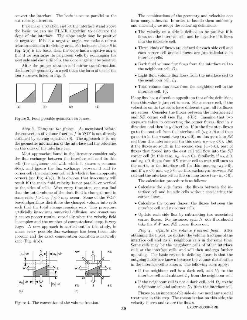
After the proper rotation and mirror transformation,the interface geometry in a cell takes the form of one of thefour subcases listed in Fig. 3.
Figure 3. Four possible geometric subcases.
Step 3. Compute the fluxes. As mentioned before,the convection of volume fraction f in VOF is not directlyobtained by solving equation (9). The approach is to usethe geometric information of the interface and the velocitieson the sides of the interface cell.
Most approaches found in the literature consider onlythe flux exchange between the interface cell and its sidecell (the neighbour cell with which it shares a commonside), and ignore the flux exchange between it and itscorner cell (the neighbour cell with which it has an oppositecorner) (see Fig. 4(a)). It is obvious that inaccuracy willresult if the main fluid velocity is not parallel or verticalto the sides of cells. After every time step, one can findthat the total volume of the dark fluid is changed, and insome cells, f > 1 or f < 0 may occur. Some of the VOF-based algorithms distribute the changed volume into cellssuch that the total change remains zero. This procedureartificially introduces numerical diffusion, and sometimesit causes poorer results, especially when the velocity fieldis complex and the number of computational steps is verylarge. A new approach is carried out in this study, inwhich every possible flux exchange has been taken intoaccount and the exact conservation condition is naturallykept (Fig. 4(b)).
Figure 4. The convection of the volume fraction.
The combinations of the geometry and velocities canform many subcases. In order to handle them uniformlyand efficiently, we adopt the following definitions.
• The velocity on a side is defined to be positive if itflows out the interface cell, and be negative if it flowsinto the interface cell.
• Three kinds of fluxes are defined for each side cell andeach corner cell and all fluxes are just calculated ininterface cells.
• Dark fluid volume flux flows from the interface cell tothe neighbour cell, Df .
• Light fluid volume flux flows from the interface cell tothe neighbour cell, Lf .
• Total volume flux flows from the neighbour cell to theinterface cell, Vf .
If any flux has a direction opposite to that of the definition,then this value is just set to zero. For a corner cell, if thevelocities on its two sides have different signs, all its fluxesare zeroes. Consider the fluxes between the interface celland SE corner cell (see Fig. 4(b)). Imagine that twosteps are taken in convecting the corner fluxes, first in xdirection and then in y direction. If in the first step fluxesgo to the east cell from the interface cell (uE > 0) and thengo north in the second step (uS < 0), no flux goes into SEcell from this interface cell (in this case, uE ·uS < 0). Butif the fluxes go south in the second step (uS > 0), part offluxes that flowed into the east cell will flow into the SEcorner cell (in this case, uE ·uS > 0). Similarly, if uE < 0,and uS < 0, fluxes from SE corner cell to west will turn tothe north, to the interface cell (in this case, uE ·uS > 0),and if uE < 0 and uS > 0, no flux exchanges between SEcell and the interface cell in this circumstance (uE ·uS < 0).
The calculation procedure is as follows:
• Calculate the side fluxes, the fluxes between the in-terface cell and its side cells without considering thecorner fluxes.
• Calculate the corner fluxes, the fluxes between theinterface cell and its corner cells.
• Update each side flux by subtracting two associatedcorner fluxes. For instance, each N side flux shouldtake the NW and NE corner fluxes out.
Step 4. Update the volume fraction field. Afterobtaining the fluxes, we update the volume fractions of theinterface cell and its all neighbour cells in the same time.Some cells may be the neighbour cells of other interfacecells or the interface cells, and will then undergo furtherupdating. The basic reason in defining fluxes is that theoutgoing fluxes are known because the volume distributionin the interface cell is known. The following rules apply:
• If the neighbour cell is a dark cell, add Vf to theinterface cell and subtract Lf from the neighbour cell.
• If the neighbour cell is not a dark cell, add Df to theneighbour cell and subtract Df from the interface cell.
Fluxes on an impermeable side do not need any specialtreatment in this step. The reason is that on this side, thevelocity is zero and so are the fluxes.
39 EX5031-000004-TRB
4. Results and Discussion
4.1 Validation Tests
The accuracy and reliability of the numerical methods usedin this work have been tested in many ways. Two globalparameters are always monitored:global velocity-divergence,
δm =∑
all cells
|∆u1∆x2 +∆u2∆x1|
and total dark fluid volume,
Vd =∑
all cells
f∆x1∆x2
In our computations, the global velocity-divergence iscontrolled in less than 10−2. When f is set to zero ineach cell, then the problem reduces to uniform fluid case.In this way, we compared our results with Ertekin [21]at Re=5000 and Dennis [22] at Re=100. (To comparewith Ertekin’s results, we modified the free surface condi-tion to nonslip boundary condition.) We found excellentagreement with both works.
To check the VOF scheme, many cases have beentested. The fluctuation of the global parameter Vd is lessthan 0.01% after every 1000 time steps when we applya given divergence-free velocity field. This error is justcaused by the single precision round-off error. Due tospace limitations, only two tests are discussed below. Toverify the results, we will suppose two fluids have the samephysical properties. Case 1 is free convection of a dark-fluid circle. In this test, the velocity field is specified to beuniform, so it is exactly divergence-free. In this way, wecan focus our attention on the VOF scheme itself. Differentvelocity orientations against the grids were tested. In Fig.5, the original circle has a diameter of 15 cells, and thevelocity field is given by u1 =1, u2 =−1. After 1000 timesteps, the dark circle keeps the perfect circle shape and itsvolume only changes 0.003%.
Figure 5. Free convection of a circle. Time t and totaldark fluid volume Vd are dimensionless. Reference timeand volume are unspecified for general case.
Case 2 is similar to a flow visualization experiment.In the upstream, three layers of dark fluid flow into the
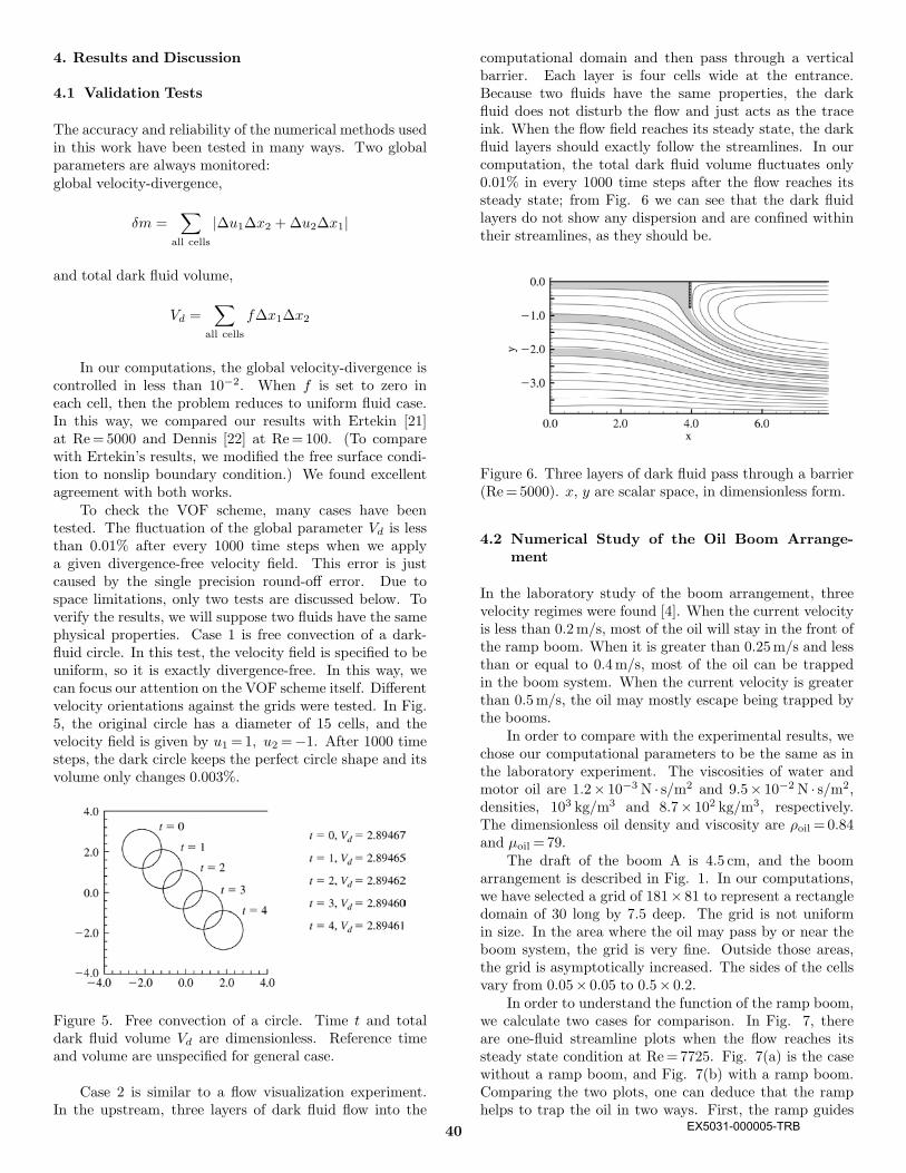
computational domain and then pass through a verticalbarrier. Each layer is four cells wide at the entrance.Because two fluids have the same properties, the darkfluid does not disturb the flow and just acts as the traceink. When the flow field reaches its steady state, the darkfluid layers should exactly follow the streamlines. In ourcomputation, the total dark fluid volume fluctuates only0.01% in every 1000 time steps after the flow reaches itssteady state; from Fig. 6 we can see that the dark fluidlayers do not show any dispersion and are confined withintheir streamlines, as they should be.
Figure 6. Three layers of dark fluid pass through a barrier(Re=5000). x, y are scalar space, in dimensionless form.
4.2 Numerical Study of the Oil Boom Arrange-ment
In the laboratory study of the boom arrangement, threevelocity regimes were found [4]. When the current velocityis less than 0.2m/s, most of the oil will stay in the front ofthe ramp boom. When it is greater than 0.25m/s and lessthan or equal to 0.4m/s, most of the oil can be trappedin the boom system. When the current velocity is greaterthan 0.5m/s, the oil may mostly escape being trapped bythe booms.
In order to compare with the experimental results, wechose our computational parameters to be the same as inthe laboratory experiment. The viscosities of water andmotor oil are 1.2× 10⁻³ N · s/m2 and 9.5× 10⁻² N · s/m2,densities, 103 kg/m3 and 8.7× 10² kg/m3, respectively.The dimensionless oil density and viscosity are ρoil =0.84and µoil =79.
The draft of the boom A is 4.5 cm, and the boomarrangement is described in Fig. 1. In our computations,we have selected a grid of 181× 81 to represent a rectangledomain of 30 long by 7.5 deep. The grid is not uniformin size. In the area where the oil may pass by or near theboom system, the grid is very fine. Outside those areas,the grid is asymptotically increased. The sides of the cellsvary from 0.05× 0.05 to 0.5× 0.2.
In order to understand the function of the ramp boom,we calculate two cases for comparison. In Fig. 7, thereare one-fluid streamline plots when the flow reaches itssteady state condition at Re=7725. Fig. 7(a) is the casewithout a ramp boom, and Fig. 7(b) with a ramp boom.Comparing the two plots, one can deduce that the ramphelps to trap the oil in two ways. First, the ramp guides
40 EX5031-000005-TRB

the direction of the flow. When the fluid enters the oilcollection zones, it will have a lower vertical downwardvelocity, and the oil will be prevented from overshootingout of these zones. Another reason is that a large quiescentoil collection zone is created by the ramp boom. As aresult, in the presence of the ramp boom, the buoyant forcehas a longer action time to separate the fluids due to theirdifferent densities.
Figure 7. Streamline plots of one-fluid cases. x, y arescaled by the draft (L=4.5 cm) of boom A.
Figure 8. Initial condition for the following computationalcases (at t=0). x, y are scaled by the draft (L=4.5 cm) ofboom A.
Figure 9. The oil layer evolution with current velocity of 0.2m/s. x, y are scaled by the draft (L=4.5 cm) of boom A, andthe corresponding times are 1.125 s, 2.250 s, 3.375 s, 4.5 s, 6.75 s, and 9.0 s, respectively.
In the following section we present the computationalresults of several current velocities. From their definitions,Reynolds number and Froude number are directly pro-portional to the current velocity when other physical pa-rameters remain unchanged: Re=38625.0U0, Fr=1.505U0
where U0 is the current velocity, and it has the unit ofmeter per second. The initial condition is the same foreach following computational case (Fig. 8).
With the current velocity U0 =0.2m/s, the dimension-less parameters are Re=7725 and Fr=0.301. It appearsfrom Fig. 9 that the oil inertia cannot overcome the buoy-ancy when it moves along the ramp boom. The oil goesforward first and then goes backward. Only a little oilenters collection zone C1; most of the oil stays in the frontof the ramp. A head wave is formed against the currentin the oil layer. This head wave was also found in exper-imental investigation [4, 23]. Under the influence of thebuoyancy, the oil has a tendency to move up and stretchout on the free surface, but the inertia of the oil and thefriction between water and oil make the oil follow the watercurrent. These opposite actions cause the head wave in thefront of the oil layer.
On the interface near the head wave, there is a strongshear layer. The oil may form little droplets and enter thewater current owing to turbulence and Kelvin-Helmholtzeffect. This is the so-called entrainment failure of oilcontainment by boom [24]. The entrainment failure occursin small space and time scales; it is not included in thisstudy.
When the current velocity increases to 0.25m/s, thesituation is very different. All of the oil passes through theramp boom and most of the oil is collected by zone C1 andC2. Fig. 10 also shows that the oil is broken into piecesand the interface is totally deformed when time is less than30. But at time=40, the oil stays at the top in differentcollection zones; the oil and water are well separated
41 EX5031-000006-TRB
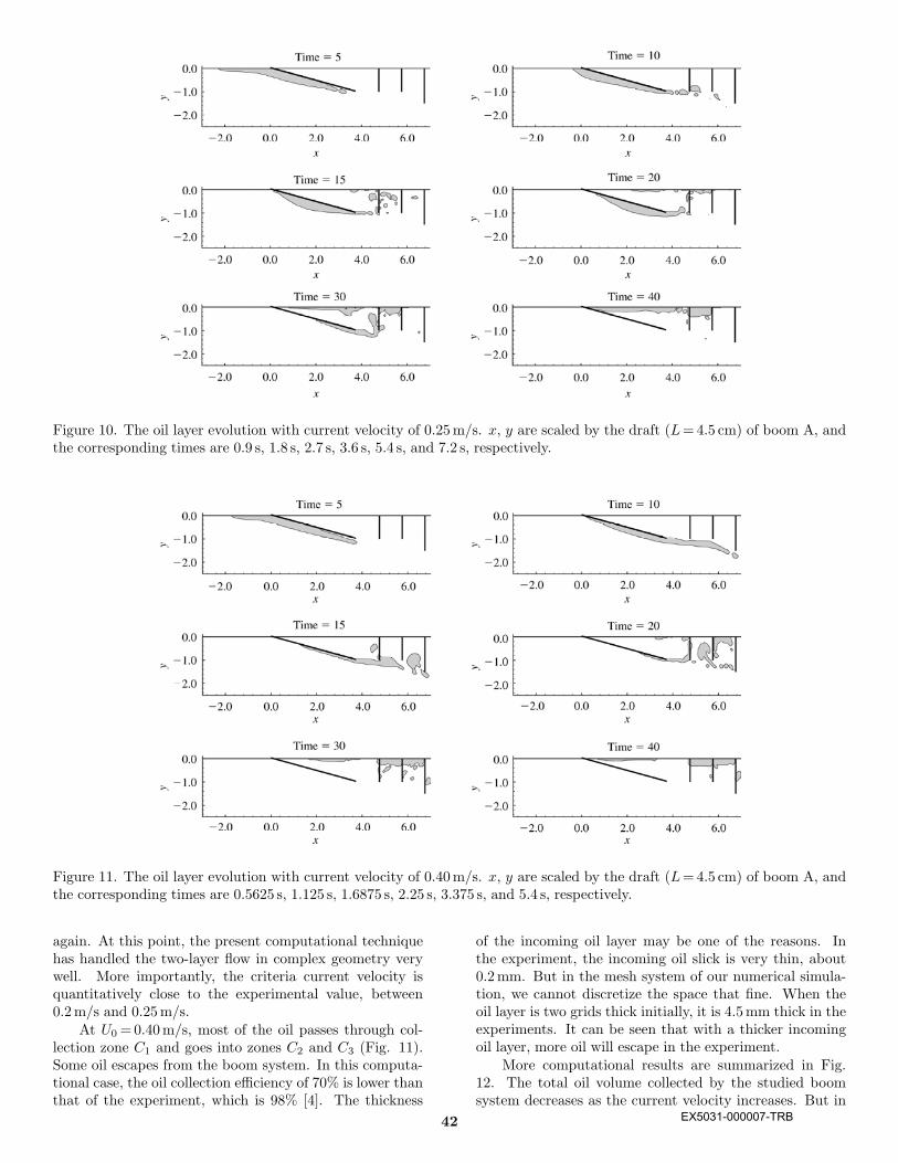
Figure 10. The oil layer evolution with current velocity of 0.25m/s. x, y are scaled by the draft (L=4.5 cm) of boom A, andthe corresponding times are 0.9 s, 1.8 s, 2.7 s, 3.6 s, 5.4 s, and 7.2 s, respectively.
Figure 11. The oil layer evolution with current velocity of 0.40m/s. x, y are scaled by the draft (L=4.5 cm) of boom A, andthe corresponding times are 0.5625 s, 1.125 s, 1.6875 s, 2.25 s, 3.375 s, and 5.4 s, respectively.
again. At this point, the present computational techniquehas handled the two-layer flow in complex geometry verywell. More importantly, the criteria current velocity isquantitatively close to the experimental value, between0.2m/s and 0.25m/s.
At U0 =0.40m/s, most of the oil passes through col-lection zone C1 and goes into zones C2 and C3 (Fig. 11).Some oil escapes from the boom system. In this computa-tional case, the oil collection efficiency of 70% is lower thanthat of the experiment, which is 98% [4]. The thickness
of the incoming oil layer may be one of the reasons. Inthe experiment, the incoming oil slick is very thin, about0.2mm. But in the mesh system of our numerical simula-tion, we cannot discretize the space that fine. When theoil layer is two grids thick initially, it is 4.5mm thick in theexperiments. It can be seen that with a thicker incomingoil layer, more oil will escape in the experiment.
More computational results are summarized in Fig.12. The total oil volume collected by the studied boomsystem decreases as the current velocity increases. But in
42 EX5031-000007-TRB

Figure 12. Oil volume collected by zones versus currentvelocity. Oil volume in a collection zone is the summationof f∆x∆y in this zone. Total collected oil includes the oil incollection zones 1, 2, and 3, and the oil in front of the ramp.Oil volume is dimensionless scaled by L×L=20.25 cm2,in the 2-D calculations.
each of three separated collection zones, the oil volume hasa peak value at a certain current velocity. The peak valuein the last zone appears when the current velocity is near0.4m/s. In some sense, that oil passing through the rampboom is similar to throwing an object under the influenceof the gravity. If the shooting angle is fixed, the higher thevelocity, the longer the landing distance. When this kindof landing point is on the outside of the last boom, mostof the oil will escape. This is the reason that the totalcollected oil volume decreases quickly when the currentvelocity exceeds 0.40m/s.
We can then arrange the booms by a longer separateddistance and find a suitable attack angle for the ramp boomto achieve a good performance. But in fact two neighbour-ing booms cannot be separated too widely; otherwise, thestill zones will no longer exist and the collected oil willre-enter the current. Moreover, the effects of the densityand viscosity of the oil and the depth of the canal makethis problem much more complicated than the problem ofthrowing an object.
5. Conclusion
An advanced interface convection technique in complexgeometry has been developed and applied to analyze an oilboom arrangement design. This technique is based on thenumerical volume-of-fluid method. The volume fractionconvection is conservative and accurate in nature; no ad-ditional artificial correction is necessary. The conceptualinterface basis and three types of fluxes are introducedto handle the possible combinations of complex interface
geometry and the velocity field. These definitions makethis VOF algorithm easy to use. By using this scheme,we preliminarily studied the performance of an oil boomarrangement. Our computation shows that the ramp boomcreates a flow pattern for trapping the oil slick in the oilcollection zone. Three velocity regimes, which have beenfound in the laboratory experiments, are also found in ournumerical simulations, and the critical velocities obtainedfrom the experiment [4] and our computations agree witheach other. The successful primary study shows that thisVOF scheme can be used in the computer-aided boomarrangement design and in other interface applications.
References
[1] J.-M. Lo, Laboratory investigation of single floating boomsand series of booms in the prevention of oil slick and jellyfishmovement, Ocean Engineering, 23(6), 1996, 519–531.
[2] K.V. Wong & D. Guerrero, Quantitative analysis of shorelineprotection by boom arrangements, Proc. 2nd Int. Oil SpillR&D Forum, London, May 1995.
[3] K.V. Wong & A. Wolek, Application of flow visualization to thedevelopment of an innovative boom system, Proc. 19th Arcticand Marine Oil Spill Program Technical Seminar, Calgary,Canada, June 1996.
[4] K.V. Wong & I. Kusijanovic, Oil spill recovery methods forinlets, rivers and canals, Proc. Int. Oil Spill Conf., Seattle,Washington, March 1999.
[5] M. Natori & H. Kawarada, Numerical solution of free surfacedrainage problem of two immiscible fluids by the boundaryelement method, Japanese Journal of Applied Physics, 24,1985, 1359–1362.
[6] H.C. Henderson, M. Kok, & W.L. de Koning, Computer-aided spillway design using the boundary element method andnon-linear programming, International Journal of NumericalMathematical Fluids, 13, 1991, 625–641.
[7] D.R. Lynch, Unified approach to simulation on deformingelements with application to phase change problems, Journalof Computational Physics, 47, 1982, 387–411.
[8] P. Bach & O. Hassager, An algorithm for the use of theLagrangian specification in Newtonian fluid mechanics andapplications to free-surface flow, Journal of Fluid Mechanics,152, 1985, 173–190.
[9] G. Ryskin & L.G. Leal, Numerical solution of free-boundaryproblems in fluid mechanics, Part 1: The finite-differencetechnique, Journal of Fluid Mechanics, 148, 1984, 1–17.
[10] N.S. Asaithambi, Computation of free-surface flows, Journalof Computational Physics, 73, 1987, 380–394.
[11] S. Osher & J.A. Sethian, Fronts propagating with curvature-dependent speed: Algorithms based on Hamilton-Jacobi for-mulations, Journal of Computational Physics, 79, 1988, 12–49.
[12] M. Sussman, P. Smereka, & S. Osher, A level set approach forcomputing solutions to incompressible two-phase flow, Journalof Computational Physics, 114, 1994, 146–159.
[13] R.K.-C. Chan & R.L. Street, A computer study of finite-amplitude water waves, Journal of Computational Physics, 6,1970, 68–94.
[14] H. Miyata, Finite difference simulation of breaking waves,Journal of Computational Physics, 65, 1986, 179–214.
[15] A.J. Chorin, Curvature and solidification, Journal of Compu-tational Physics, 57, 1985, 472–490.
[16] D.L. Young, Time-dependent multi-material flow with largefluid distortion, in K.W. Morton & M.J. Baineks (Eds.),Numerical methods for fluid dynamics (New York: AcademicPress, 1982).
[17] N. Ashgriz & J.Y. Poo, FLAIR: Flux line-segment model foradvection and interface reconstruction, Journal of Computa-tional Physics, 93, 1991, 449–468.
[18] S.-O. Kim & H.C. No, Second-order model for free surfaceconvection and interface reconstruction, International Journalfor Numerical Methods in Fluids, 26, 1998, 79–100.
43 EX5031-000008-TRB

[19] E.G. Puckett, A.S. Almgren, J.B. Bell, D.L. Marcus, & W.J.Rider, A high-order projection method for tracking fluid in-terface in variable density incompressible flows, Journal ofComputational Physics, 130, 1997, 269–282.
[20] S.V. Patankar, Numerical heat transfer and fluid flow (Wash-ington, DC: Hemisphere Publishing, 1979).
[21] R.C. Ertekin & H. Sundararaghavan, The calculations of theinstability criterion for a uniform viscous flow past an oil boom,Journal of Offshore Mechanics and Arctic Engineering, 117,1995, 24–29.
[22] S.C.R. Dennis, O. Wang, M. Coutanceau, & J.-L. Launay,Viscous flow normal to a flat plate at moderate Reynoldsnumbers, Journal of Fluid Mechanics, 248, 1993, 605–635.
[23] G.A.L. Delvigne, Barrier failure by critical accumulation ofviscous oil, Proc. Int. Oil Spill Conf., USEPA, USCG, andAPI, San Antonio, TX, 1989, 143–148.
[24] S.T. Grilli, Z. Hu, & L.S. Malcolm, Numerical modeling of oilcontainment by a boom, Proc. 19th Arctic and Marine Oil SpillProgram Technical Seminar, Calgary, Canada, 1996, 343–376.
Biographies
Jianzhi Fang currently workswithin the IT industry in theMiami area.
Kau-Fui Wong has been a pro-fessor for almost 26 years. In theoil spill community he is popu-larly known as “Dr. Boom.” Hisresearch interests are energy andthe environment, and recently hehas developed an interest in nan-otechnology.
44 EX5031-000009-TRB

Reproduced with permission of the copyright owner. Further reproduction prohibited without permission.
EX5031-000010-TRB