An Aerodynamic Analysis of Recent FIFA World Cup Balls

Adrian L. Kiratidis∗ and Derek B. Leinweber†

Special Research Centre for the Subatomic Structure of Matter, Department ofPhysics, The University of Adelaide, SA, 5005, Australia.

February 20, 2018

Abstract

Drag and lift coefficients of recent FIFA world cup balls are examined. We fit a novelfunctional form to drag coefficient curves and in the absence of empirical data provide estimatesof lift coefficient behaviour via a consideration of the physics of the boundary layer. Differencesin both these coefficients for recent balls, which result from surface texture modification, cansignificantly alter trajectories. Numerical simulations are used to quantify the effect thesechanges have on the flight paths of various balls. Altitude and temperature variations atrecent world cup events are also discussed. We conclude by quantifying the influence thesevariations have on the three most recent world cup balls, the Brazuca, the Jabulani and theTeamgeist. While our paper presents findings of interest to the professional sports scientist, itremains accessible to students at the undergraduate level.

1 Introduction

The aerodynamics of various sports balls has been an area of long-standing interest for both thegeneral public [1–5] and the professional sports scientist [6–8]. Golf balls [9,10], cricket balls [11,12],baseballs [13, 14] and spheres more generally [15, 16] have all been areas of research interest. Ofall the sports balls, there is more worldwide interest in the aerodynamics of football (soccer) ballsthan any other. This interest typically peaks around the time of the FIFA World Cup and it isnot hard to see why.

The FIFA World Cup is perhaps the most watched sporting event globally. According to FIFA,more than 3.2 billion people, or almost half the world’s population watched at least part of the2010 incarnation [17], which netted FIFA $885 million US dollars in broadcasting and marketingrights [18]. The 2014 World Cup also broke numerous viewing records in a number of differentregions [19]. With the eyes of the media world on the competition there is never a shortageof controversy, both on and off the field. One such topic that has caused controversy in recenttimes is that of the ball, where the aerodynamic properties of the surface of the ball has played acontroversial role.

In 1978 the unmistakable ‘Tango’ design was developed for the world cup in Argentina. Theball was made of leather with a waterproofing coating, and had 20 panels with the visually iconic‘triads’ creating the impression of 12 circles. A Tango type ball was used until 2002, when theball manufacturers, Adidas, opted for a change. The 32 Panel Adidas Fevernova, with its thickpolyurethane surface which included a layer of purpose built foam was designed. It was builtfor a ‘more precise and predictable flight path’, and yet the controversy came. Legendary Italianshot-stopper Gianluigi Buffon labelled the Fevernova “a ridiculous kiddy’s bouncing ball”, whilethe Brazilian star Rivaldo told reporters the ball soars too far when kicked.

For the 2006 FIFA world cup in Germany the ball was the 14 Panel Teamgeist. Its thermallybonded panels represented a rather radical change when compared to the stitched panels seen in

∗Email: adriankiratidis@gmail.com; Corresponding author†Email: derek.leinweber@adelaide.edu.au

1

arX

iv:1

710.

0278

4v2

[ph

ysic

s.po

p-ph

] 1

8 Fe

b 20

18

previous balls. The Teamgeist was the roundest ball to date, had very smooth panels and wasessentially water-proof. It was expected to perform more uniformly and predictably, but onceagain the complaints came. Germany’s keeper Oliver Kahn said the ball was “built in favour ofthe strikers”, while Brazilian Roberto Carlos, who has his fair share of famous strikes to his name,said “It’s very light, the way they are doing it is completely different from before. It seems like it’smade of plastic.”

The 2010 FIFA World Cup in South Africa then brought us the most controversial ball todate, the Jabulani. The surface of the ball was constructed with 8 thermally bonded panels, eachpossessing a microtexture. The criticism this time was especially widespread. Brazilian keeperJulio Cesar said “It’s terrible, horrible. It’s like one of those balls you buy in the supermarket”while the English custodian Joe Hart described it doing “anything but staying in my gloves”.Outfield players were also critical. The Dane Daniel Agger said “it makes us look like drunkensailors” while even the Brazilian forward Robinho said “For sure the guy who designed this ballnever played football”. Its general reception by most players was sufficiently negative to promptboth FIFA and Adidas to release official comments on the ball, along with a promise for furtherdialogue. This was an unprecedented measure. There were however some memorable goals scoredwith the ball, perhaps none more than Maicon’s goal in the group stage against North Korea [20],in which the ball is seen to swerve significantly over a relatively short distance.

The recent 2014 FIFA World Cup has come and gone, and the official match ball, the “Brazuca”,with its 6 thermally bonded panels has undoubtedly been put under heavy scrutiny by the play-ers. Given the extensive criticism received by previous world cup balls, perhaps one wouldn’t besurprised to hear a raft of complaints levelled at the Brazuca. However, while there was certainlycontroversy on the field, there was generally praise for the ball, with the international media largelyfocusing on on-field issues. With the 2014 Brazuca seemingly a well-received ball, the fans couldeasily be left wondering why there were so many complaints at previous world cups. Were theplayer’s complaints valid with previous balls being, in some sense, “horrible”, or is it simply aneasy excuse to use the ball as a scapegoat for any failures, past or potential? A discussion of thephysics involved in the ball’s flight will shed light on an answer to such questions.

In this paper we examine the aerodynamics of the three most recent world cup balls, theTeamgeist, the Jabulani and the Brazuca, comparing their aerodynamic properties to the 32-panelballs players are accustomed to from various leagues around the world. We begin in Section 2by outlining the basic physics at work as a ball flies through the air. We then introduce a newfunctional form in order to fit drag coefficient (CD) data in Section 3. Using these fits and ourunderstanding of the physics of the boundary layer we then discuss the implications for the liftcoefficient (CL) of the ball in section 4, making use of empirical lift coefficient data where available.In doing so, we develop a method to estimate the behaviour of lift coefficients in the absence ofreadily available empirical data, enabling us to produce accurate flight trajectories. The effectaltitude and temperature has on flight paths is then quantified in Section 5, where we focus on thetwo most recent world cup balls. Finally throughout Section 7 we present visualisations comparingflight trajectories with a variety of different balls and various initial conditions.

2 Fundamental Ball Aerodynamics

As a ball flies through the air it is subject to forces due to gravity and the air through which itis flying. We follow the usual practice [21–23] of separating the force exerted by the air into dragand lift forces, FD and FL respectively, as shown in Fig. 1.

For a given ball the drag force is in a direction opposite to the ball’s velocity and has magni-tude [24]

FD =1

2CD(Re, Sp) ρAv2, (1)

while the lift force, or Magnus force, is in the direction ~ω × ~v and has magnitude [24]

FL =1

2CL(Re, Sp) ρAv2. (2)

2

&%'$

����������3

JJJJJJJJJ]

���

���

��

��+

?

I

v

θ

FG = mg

FD

FL

Figure 1: A schematic diagram of the forces on a ball travellingwith velocity v at angle θ to the ground (magnitudes are of coursenot to scale). Here the lift force is drawn for backspin, ~ω, with thespin axis orthogonal to the plane of the page and pointing out ofthe page.

Here ~ω is the ball’s angular velocity, v is the magnitude of the ball’s velocity, ~v, ρ is the airdensity, and A is the ball’s cross sectional area. CD and CL are the ball’s drag and lift coefficientsrespectively. It’s interesting to note that the lift force was first observed by Robins [25] in measuringthe trajectories of spinning projectiles. Reference [26] provides a contemporary review.

These coefficients are functions of Reynolds number Re, and spin parameter Sp, where

Re :=v D

νk, (3)

andSp :=

r ω

v. (4)

Here r is the ball’s radius, D = 2r its diameter and ω its angular speed, |~ω|. νk is the kinematicviscosity which is given by the ratio of viscosity to air density. Crucially, CD and CL are alsodependent on the ball’s surface properties [6, 7, 15, 16] via the physics of the thin layer of airaround the ball, called the boundary layer. At low speeds, in the laminar airflow regime, theboundary layer separates early creating a large wake with high drag (high CD) as shown in part a)of Figure 2. On the other hand, at high speeds, in the turbulent airflow regime, the boundary layerseparates late from the ball creating a small wake and hence low drag (small CD) as seen in partb) of Figure 2. Wind tunnel visualisations of this effect can be found in references [27, 28]. Thespeed at which this turbulent-to-laminar transition occurs, called the critical Reynolds number,is directly affected by the surface roughness of the ball. It has been shown for spheres that highlevels of surface roughness correspond to a relatively low critical Reynolds number [16]. Thissurface roughness serves to trip turbulence, delaying the onset of the laminar regime as the ballslows. However, the same roughness also serves to increase drag in the turbulent regime, by virtueof thickening the boundary layer. The critical speed at which the turbulent-to-laminar transitionoccurs can have wide-reaching consequences for a ball’s aerodynamic performance, introducing thepossibility of surprising even the game’s best goalkeepers. This is discussed in more depth for eachball individually in Section 3.

3

(a) A diagram showing the boundary layer sepa-rating early in the low speed and high drag lam-inar flow regime creating a large wake.

(b) A diagram showing the boundary layer sep-arating late in the high speed and low drag tur-bulent flow regime creating a small wake.

Figure 2: (Colour online) Diagrams showing boundary layer separation for laminarand turbulent regimes.

The turbulent-to-laminar transition is not the only difficulty goalkeepers have to contend with.A common technique when shooting for goal is to impart spin on the ball in order to perform aswerving shot. A spinning ball drags the boundary layer with it resulting in later boundary layerseparation on one side of the ball than the other, creating an uneven wake as shown in Figure 3.This uneven boundary layer separation unbalances the side forces on the ball contributing to theMagnus force, and hence to the swerve of the ball. In the ball’s reference frame the air in theboundary layer is travelling at v v − rω on one side and v v + rω on the other. By the Bernoulliprinciple faster flowing air creates a region of lower pressure, meaning a spinning ball will create apressure gradient pulling the ball further “towards its nose”. The pressure gradient and the unevenboundary-layer separation work together to produce a strong side force. While back-spinning ballsexperience lift, side-spinning balls swerve. In both cases it is common to refer to this Magnus forceas a lift force.

Furthermore, at low drag, the boundary layer is close to the ball being well intact, enhancingthe aforementioned lift affects, whereas at high drag a thicker boundary layer that has been spoiledwill result in a reduction. Consequently, the ball’s surface roughness is once again intimately linkedto its aerodynamic performance.

Total seam length and depth are currently believed to be the dominant measures of surfaceroughness for footballs [29]. Of the balls studied for this work the Jabulani has the lowest totalseam length of v 203 cm while the seam lengths of the Brazuca and Teamgeist are v 327 cm andv 345 cm respectively [30]. Conventional 32-panel balls have a seam length of v 400 cm [29, 30].In addition to having the shortest seam length the Jabulani also has the most shallow seams ofv 0.48 mm, while a conventional 32-panel ball’s seams are v 1.08 mm deep [30] and the Brazucahas the largest value of v 1.56 mm. This makes the Jabulani the smoothest of all the balls,meaning it will have the highest critical Reynolds number. Given the seam lengths and depths ofthe 2014 Brazuca and 32-panel balls above, we would anticipate them to have similar aerodynamicproperties.

Currently, the sport’s world governing body, FIFA, has relatively tight restrictions on multipleball properties, such as circumference, mass and initial pressure of the ball [31]. However, there areno such regulations on the surface roughness or material used for the ball’s construction, enablingball manufacturers to alter CD and CL. For a given ball CD and CL can be determined empirically,either through trajectory analysis [21,22,32,33] or by analysing wind tunnel data [27,34].

3 Drag Coefficients

To create accurate flight trajectories it is essential to quantify the drag and lift coefficients in amanner that captures all the physics governing their behaviour. Motivated by wind tunnel data [8]

4

Figure 3: (Colour online) A diagram showing the boundary layer properties around arotating ball. The lighter shading of the boundary layer represents the lower pressureof the Bernoulli effect.

for the CD dependence on Reynolds number for various non-spinning balls, we propose a new termin the CD fitting function used by [22,35]. The new fitting function (at Sp = 0), is given by

CD(v)∣∣Sp=0

=a− bmin

1 + exp[(v − vc)/vs]+ bmin +

v − vmin1 + exp[−(v − vmin)/vs]

bmax − bminvmax − vmin

, (5)

where the third term is a new term constructed in order to reproduce the increase in drag athigh Reynolds numbers [8]. Given that goal scoring shots are likely to spend a significant portionof their flight path in this region, the third term is a useful addition. We note here that thecomplete functional form and all coefficients are chosen in order to characterise the degrees offreedom required to reproduce a close fit to available data such as the wind tunnel results seenin reference [8] without over-fitting. Therefore, each coefficient has a corresponding attribute itgoverns, which we now proceed to describe.

The variable a governs the maximum value attained by CD for the given ball, vc governs thecritical velocity at which the turbulent-to-laminar transition occurs and vs governs the slope andhence relative speed of the associated transition. The variables (bmin, bmax) and (vmin, vmax)control the minimum and maximum CD values and velocities respectively of the linear tail of thefunction in the turbulent regime.

Fits of Equation 5 to available wind tunnel data are illustrated in Figure 4. Figure 5 confirmsour expectations based on boundary layer physics and surface roughness as discussed in Section2. As the Jabulani has the shortest total seam length and the shallowest seams, the turbulent-to-laminar transition occurs at the highest speed. This effect is significant and easily observedin Figure 4. Although a typical goal scoring shot would likely begin its trajectory at about 35ms−1, some shots could slow to as low as v 15 ms−1, meaning a portion of the trajectory is spenttransitioning from turbulent to laminar boundary layer flows. The Tango12 32-panel ball is nextto undergo the transition to laminar flow followed closely by the Brazuca and Teamgeist. This isin accord with our expectations based on surface roughness in Section 2.

During the turbulent-to-laminar transition, the airflow on one side of the ball may be slowenough to be laminar, while a seam or surface roughness may be tripping turbulence in the bound-ary layer on the opposite side. The boundary layer on the turbulent side will separate later, givingrise to an uneven wake and hence a lift force. As the ball is travelling at a speed in the critical regiona small change in seam orientation may reverse the uneven wake with the ball now experiencinga lift force in the opposite direction. It is exactly this type of erratic behaviour that makes a ball

5

5 10 15 20 25 30 35v (m/s)

0.1

0.2

0.3

0.4

0.5

CD

Brazuca Drag Coefficient

(a) The fit to Brazuca drag coefficient data. Datapoints were obtained from wind tunnel experi-ments [37]. Values have been averaged over twoseam orientations.

5 10 15 20 25 30 35v (m/s)

0.1

0.2

0.3

0.4

0.5

CD

Jabulani Drag Coefficient

(b) The fit to Jabulani drag coefficient data.Data points were obtained from wind tunnel ex-periments [37]. Values have been averaged overtwo seam orientations.

5 10 15 20 25 30 35v (m/s)

0.1

0.2

0.3

0.4

0.5

CD

Teamgeist Drag Coefficient

(c) The fit to Teamgeist drag coefficient data.Data points were obtained via trajectory analy-sis [22].

5 10 15 20 25 30 35v (m/s)

0.1

0.2

0.3

0.4

0.5

CD

Tango12 Drag Coefficient

(d) The fit to Tango 12 drag coefficient data.Data points were obtained from wind tunnel ex-periments [37]. Recall the Tango 12 is a 32-panelball.

Figure 4: (Colour online) Diagrams showing various drag coefficient data and theirfits via Eq. 5.

susceptible to knuckle-ball type effects that are well known from sports such as baseball [14, 36].In this way the critical Reynolds number can be thought of as a characteristic speed near whichthe flight path of the ball becomes unpredictable.

As shown in Figures 4 and 5, this characteristic range of speeds varies from ball to ball. For theJabulani this unpredictable region lies approximately between 15 − 24 ms−1, while the the otherballs have their corresponding region at approximately 10 − 17 ms−1. Recall that while shots atgoal can start their flight paths at speeds of up to 35 ms−1 just after the ball leaves the player’sboot, the ball can slow to between 15 − 20 ms−1 by the time the ball arrives at the goaline andthe keeper is called to make a save.

This is precisely the reason for the much publicised complaints about the Jabulani. Its un-predictable region where it was susceptible to knuckle-ball type effects happens to coincide withthe typical speeds the ball was travelling at just before it arrived at the keeper or on the head ofa striker. As the ball can slow to 15 − 20 ms−1 during relevant match situations, all balls otherthan the Jabulani generally spend their flight path in the turbulent regime, making them in somesense predictable. Furthermore, as the lift force is proportional to v2, the force on the Jabulaniwhen it starts to transition to a laminar flow is greater than that of the other balls. For example,as the Jabulani begins to transition to a laminar flow it experiences a lift force approximately(24/17)2 ≈ 2 times greater than the lift force on the Brazuca when it begins its transition. This

6

5 10 15 20 25 30 35v (m/s)

0.1

0.2

0.3

0.4

0.5

CD

Drag Coefficient Comparison

Tango12

Teamgeist

Jabulani

Brazuca

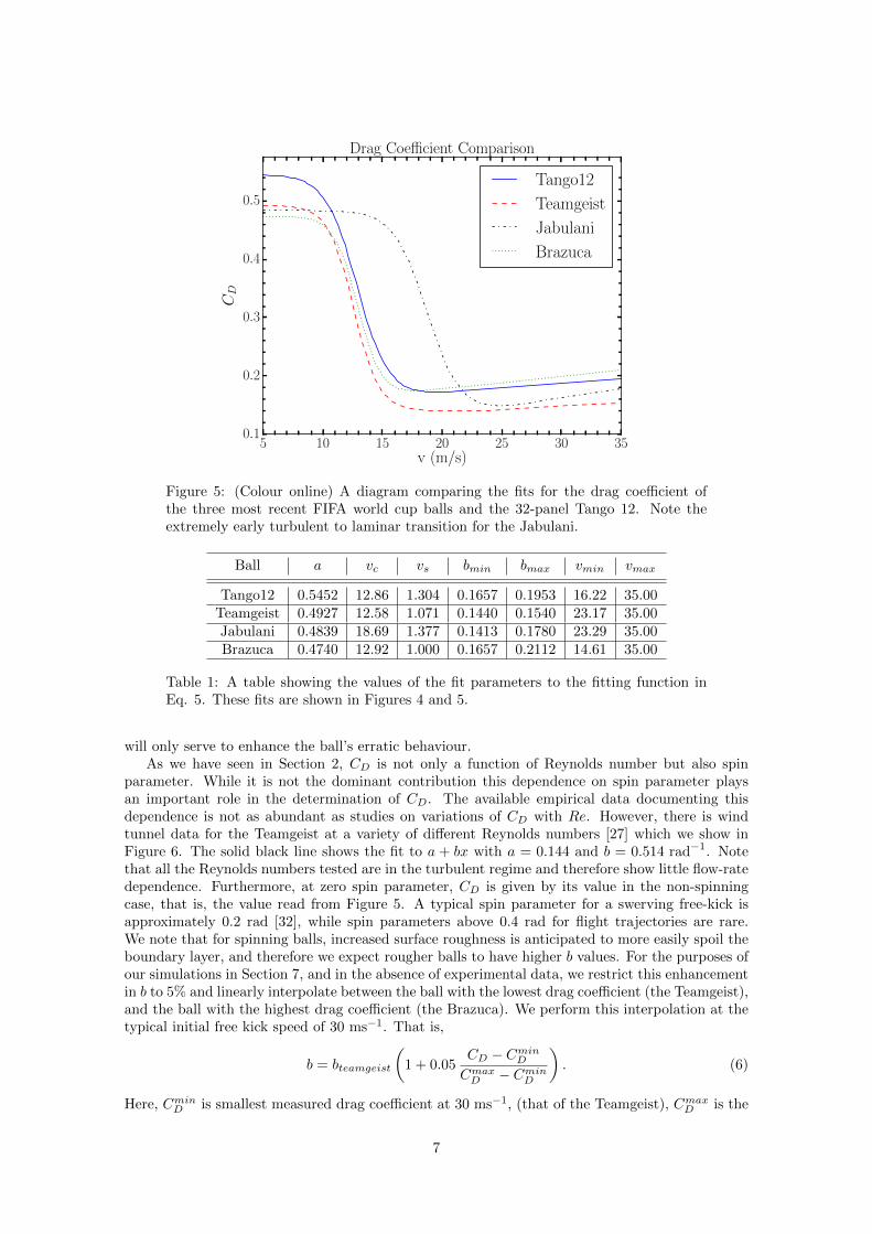
Figure 5: (Colour online) A diagram comparing the fits for the drag coefficient ofthe three most recent FIFA world cup balls and the 32-panel Tango 12. Note theextremely early turbulent to laminar transition for the Jabulani.

Ball a vc vs bmin bmax vmin vmax

Tango12 0.5452 12.86 1.304 0.1657 0.1953 16.22 35.00Teamgeist 0.4927 12.58 1.071 0.1440 0.1540 23.17 35.00Jabulani 0.4839 18.69 1.377 0.1413 0.1780 23.29 35.00Brazuca 0.4740 12.92 1.000 0.1657 0.2112 14.61 35.00

Table 1: A table showing the values of the fit parameters to the fitting function inEq. 5. These fits are shown in Figures 4 and 5.

will only serve to enhance the ball’s erratic behaviour.As we have seen in Section 2, CD is not only a function of Reynolds number but also spin

parameter. While it is not the dominant contribution this dependence on spin parameter playsan important role in the determination of CD. The available empirical data documenting thisdependence is not as abundant as studies on variations of CD with Re. However, there is windtunnel data for the Teamgeist at a variety of different Reynolds numbers [27] which we show inFigure 6. The solid black line shows the fit to a + bx with a = 0.144 and b = 0.514 rad−1. Notethat all the Reynolds numbers tested are in the turbulent regime and therefore show little flow-ratedependence. Furthermore, at zero spin parameter, CD is given by its value in the non-spinningcase, that is, the value read from Figure 5. A typical spin parameter for a swerving free-kick isapproximately 0.2 rad [32], while spin parameters above 0.4 rad for flight trajectories are rare.We note that for spinning balls, increased surface roughness is anticipated to more easily spoil theboundary layer, and therefore we expect rougher balls to have higher b values. For the purposes ofour simulations in Section 7, and in the absence of experimental data, we restrict this enhancementin b to 5% and linearly interpolate between the ball with the lowest drag coefficient (the Teamgeist),and the ball with the highest drag coefficient (the Brazuca). We perform this interpolation at thetypical initial free kick speed of 30 ms−1. That is,

b = bteamgeist

(1 + 0.05

CD − CminD

CmaxD − CminD

). (6)

Here, CminD is smallest measured drag coefficient at 30 ms−1, (that of the Teamgeist), CmaxD is the

7

0.00 0.05 0.10 0.15 0.20 0.25 0.30 0.35 0.40Sp

0.00

0.05

0.10

0.15

0.20

0.25

0.30

0.35

0.40

CD

Teamgeist Drag Coefficient vs Spin Parameter

Re = 455,172

Re = 424,827

Re = 394,482

Re = 364,137

Re = 333,793

Figure 6: (Colour online) A diagram quantifying the dependence of CD on Sp. Windtunnel data has been gleaned from reference [27]. The solid black line shows the fit.

largest measured drag coefficient at 30 ms−1, (that of the Brazuca), CD is the drag coefficient ofthe ball in question measured at 30 ms−1, while b and bteamgeist are the b values of the ball inquestion and the Teamgeist respectively. Consequently, the final value of CD, which is calculatedwith the b value from Equation 6, is then given by

CD(Re, Sp) = CD∣∣Sp=0

+ b Sp, (7)

where CD∣∣Sp=0

is set by reading the appropriate value read from Figure 5.

4 Lift Coefficients

While drag coefficient data for various balls has been well documented, there is not as muchempirical data available for lift coefficients. Nevertheless, an understanding of the physics of theboundary layer enables the relevant lift coefficient information to be related to the drag coefficients.In the turbulent regime the low drag corresponds to a small wake, meaning the boundary layeris intact. The boundary layer in this regime is therefore close to the ball enhancing the effect ofuneven boundary layer separation and pressure gradients that gives rise to lift. Balls with lowerdrag coefficients will have higher lift coefficients.

Conversely, as the ball undergoes transition to a high drag laminar flow the boundary layer isspoiled, separating much earlier creating a larger wake. Given the boundary layer is now awayfrom the ball, any uneven boundary layer separation or pressure gradient effects are diminished.A reduction in the ball’s lift coefficient occurs as it slows.

Available data supports this understanding. A compilation of relevant data from wind tunnelmeasurements and a trajectory analysis is shown in Figure 7 for the Teamgeist ball. Note that theturbulent-to-laminar transition for the Teamgeist occurs approximately between Reynolds numbersof 1.3×105 and 2.3×105, meaning all the wind tunnel data corresponding to the data points joinedby the solid lines are in the turbulent regime. The data points from the trajectory analysis are ata Reynolds number of 3× 105. We commence our discussion of Figure 7 by turning our attentionto the wind tunnel data.

There is a trend, particularly at higher values of the spin parameter, where higher Reynoldsnumbers generally correspond to lower drag. Utilizing the boundary layer discussion of this section,this is consistent with the rising tails in the drag coefficient curves of Figure 4. The Tango 12,

8

Jabulani and particularly the Brazuca all display increasing drag with increasing Reynolds numberwithin the turbulent regime. The effect is most pronounced for the Brazuca and the Jabulani whichare the balls with the most surface roughness, whereas the glassy smooth panels of the Teamgeistbetter preserve the minimum drag observed. Smooth panels preserve the boundary layer at highflow speeds whereas panel roughness acts to thicken and spoil the boundary layer [8,16]. Likewise,compromising the boundary layer compromises the lift.

As the Reynolds number is further decreased to 3× 105 we observe an enhancement to the liftcoefficient as expected. Subsequent reductions to the Reynolds number correspond to speeds duringwhich the turbulent to laminar transition is occurring, meaning the boundary layer is beginningto separate earlier. We anticipate lower lift coefficients for the “in transition” Reynolds numbersof 2.1 × 105 and 1.6 × 105. The final data point at a Reynolds number of 1.3 × 105 is now in thelaminar regime as we consequently observe the lift coefficient dropping to near zero.

Turning our discussion toward the spread of the data, we note that the variation particularlybetween the trajectory analysis data points is quite considerable. In order to obtain consistentresults from a trajectory analysis, one must orientate the ball identically between successive trials.This can be particularly difficult in practice leading to the observation of successive balls exitingthe launcher with slightly different seam orientations [22]. As previously discussed, a differingseam orientation can alter the manner in which the boundary layer separates from the ball thusaltering the lift force. The producers of these data points suggest overcoming this issue in futureexperiments by devising a method to visualise boundary layer flow during the launch. A discussionof other minor contributions to this variation can be found in reference [22].

We now draw on this understanding of the connection between drag and lift coefficients to modelthe anticipated flight trajectory of balls. In order to model the behaviour of the lift coefficients ofvarious balls, we begin by considering a power law of the form

CfitL (Sp) = αSpβ . (8)

This choice is motivated by the data in Figure 7. We choose a reference Reynolds number of 333793 at which we perform our fit, since this is the smallest Reynolds number we have data forthat remains in the turbulent regime, and consequently corresponds to the lowest CD and largestCL. As noted previously, we expect the low CD values associated with an intact boundary layer tocorrespond to high CL values and visa versa. Consequently, we aim to perform a linear interpolationup to the maximum drag coefficient, at which point the boundary layer will be completely blownaway giving rise to a lift coefficient of zero. That is, we aim to encapsulate the behaviour of CLon Sp by fitting

CL(Re, Sp) = CfitL (Sp)

(CD|Re=0 −min(CD, CD|Re=0)

CD|Re=0 − CrefD

). (9)

Here, CfitL encapsulates the power behaviour of the CL dependence on Sp displayed in Figure 7,CD|Re=0 is the drag coefficient at Re = 0 of the the ball whose data we are using to interpolate. In

our case we use the Teamgeist. CrefD is the drag coefficient evaluated at the reference spin param-eter, (which we discuss imminently) and CD is the drag coefficient of the ball we are consideringat (Re, Sp).

We note here that the drag coefficients with which we are scaling CfitL themselves depend onSp via the final term of Equation 5. Drawing from the data at the reference Reynolds numberof 333 793, we aim to achieve CL = 0.33 for Sp = 0.31, and enforce the fit to pass through(Sp,CL) = (0.19, 0.29), which we set to be our reference spin parameter. Consequently, we discover(α, β) = (1.15, 0.83) not only encapsulates the trend of reduced lift at higher flow rates in theturbulent regime, but also produces predictions for the point at Sp = 0.06 well (providing 0.14compared with the empirical value of 0.15). We therefore use these values of α and β in oursimulations.

It is evident that the empirical data contains significant uncertainties, particularly at low valuesof Sp, and future studies quantifying these uncertainties and/or increasing statistics would be usefulin producing more accurate modelling of the data.

9

0.00 0.05 0.10 0.15 0.20 0.25 0.30 0.35 0.40 0.45Sp

0.00

0.05

0.10

0.15

0.20

0.25

0.30

0.35

0.40

CL

Lift Coefficient vs Spin Parameter

Re = 455 172

Re = 424 827

Re = 394 482

Re = 364 137

Re = 333 793

Re = 300 000

Re = 210 000

Re = 160 000

Re = 130 000

Figure 7: (Colour online) A diagram showing the available lift coefficient, CL, datafor the Teamgeist. The data points joined by a solid line are wind tunnel measure-ments [27]. Data points not joined by a line are sourced from a trajectory analysis [22].

5 Altitude

In recent times the maximum altitude at which official matches can be held has been a topic ofheated discussion. This is particularly relevant on the south American continent where a significantportion of stadia are located at high elevations. The 2007 Copa Libertadores, a South Americaninternational club competition, pitted Brazilian side Flamengo against Real Potosı of Bolivia,whose home stadium is 3,960 m above sea level. Following a petition by the Brazilian FootballConfederation outlining that players were making use of bottled oxygen at such venues, FIFAimposed a ban on international matches above 2,500 m in May 2007 meaning Bolivia, Colombiaand Ecuador could no longer host World Cup qualifiers in their capital cities. This limit was laterlifted to 3,000 m meaning only Bolivia’s La Paz was effected. Ultimately however, in May 2008 theban was suspended by FIFA after an official complaint from CONMEBOL, the governing body ofsouth American football, which was supported by all member nations except Brazil.

While FIFA’s concerns were primarily about the health of the players and consequently theintegrity of the competition, altitude also has an influence on the ball’s trajectory via changingair density. As shown in Equations 1 and 2, the forces on the ball are directly proportional to airdensity which decreases with increasing altitude.

Air density, ρ, can be estimated with the ideal gas law [38]

ρ =pM

RT, (10)

where M is the molar mass, R is the ideal universal gas constant, T the temperature and p is thepressure which can be expressed as a function of elevation h as

p = p0

[1− Lh

T0

] g MRL

. (11)

Here p0 is atmospheric pressure at sea level, T0 is the temperature at sea level, g is the gravitationalacceleration and L is the temperature lapse rate, defined to be the rate at which atmospherictemperature decreases with increasing altitude. Naturally, L will vary as a result of atmospherictemperature variations. We note here that the ideal gas law is accepted as a valid approximation

10

0 500 1000 1500 2000 2500 3000 3500 4000Elevation (m)

0.7

0.8

0.9

1.0

1.1

1.2

1.3A

irD

ensi

ty(k

g/m

3)

Air Density vs Elevation in Brazil

12◦C

27◦C

(a) A plot of air density against elevation. Thetemperatures of 12◦C and 27◦C are the aver-age minimum and maximum temperatures inBras ilia during the tournament months of Juneand July. The lines at 3,600 m are shown by wayof comparison with Bolivia’s capital La Paz.

0 500 1000 1500 2000 2500 3000 3500 4000Elevation (m)

0.7

0.8

0.9

1.0

1.1

1.2

1.3

Air

Den

sity

(kg/

m3)

Air Density vs Elevation in South Africa

3◦C

18◦C

(b) A plot of air density against elevation. Thetemperatures of 3◦C and 18◦C are the averageminimum and maximum temperatures in Johan-nesburg during the tournament months of Juneand July. The lines at 3,600 m are shown by wayof comparison with Bolivia’s capital La Paz.

Figure 8: (Colour online) Plots of Air Density against altitude.

for air at Standard Temperature and Pressure (STP) of 0◦C and 101.3 kPa. At typical SouthAmerican altitudes the pressure is lower and the temperature is higher than STP, and hence theair more closely approximates an ideal gas.

In the 2014 World Cup in Brazil, the Estadio Nacional in Brasılia was the highest altitudestadium at almost 1,200m above sea level. Matches were also held in coastal cities and wereconsequently at sea level. Figure 8 a) shows the variation in air density with altitude at 12◦C and27◦C which are the average minimum and maximum temperature during the tournament months ofJune and July in Brasılia [39]. The lines at 3,600 m show the air densities at the same temperaturesin the Bolivian Capital of La Paz for comparison.

This variation is smaller than it was during the 2010 tournament. South Africa held matchesin coastal cities near sea level, while games were also played in Johannesburg at an elevationof approximately 1,750 m. Figure 8 b) shows the variation in air density with altitude at 3◦Cand 18◦C which are the average minimum and maximum temperatures during June and July inJohannesburg [39]. Once again the lines at 3,600 m are for comparison with La Paz. The effect onair density is directly proportional to the drag and lift forces and the amplitude is large with upto 23% effects observed in Figure 8 over the temperature and altitude ranges encountered.

6 Simulation Details

Prior to presenting simulation results, we here briefly outline the method by which we solve therelevant differential equations. Using Newton’s second law and the expressions for drag and liftforces in Section 2, we sum the forces on the ball to obtain the differential equation governing theball’s flight which is given by

d2~r

dt2= −g− ρAv2

2m

[CD(Re, Sp) v − CL(Re, Sp) (s× v)

]. (12)

Here is the unit vector in the y direction, v is the unit vector in the direction of the ball’s motion,and s the unit vector on the ball’s rotation axis. It is worth noting that the aerodynamic responseto surface roughness is encoded within the CD and CL coefficients discussed in Sections 2, 3 and 4.We solve this via the implementation of the iterative 5th order Cash-Karp Runge-Kutta algorithm,embedded with a 4th order approximation, enabling error estimates to be performed.

The general form for a 5th order Runge-Kutta is

yn+1 = yn + c1k1 + c2k2 + c3k3 + c4k4 + c5k5 + c6k6 +O(h6), (13)

11

where the value of ki are given by

k1 = hy′(xn, yn)

k2 = hy′(xn + a2h, yn+ b21k1)

k3 = hy′(xn + a3h, yn+ b31k1 + b32k2)

. . .

k6 = hy′(xn + a6h, yn+ b61k1 + . . .+ b65k5), (14)

h is the step size and the ai and ci coefficients are Cash-Karp parameters, which can be found(along with a more detailed discussion of the iterative method) in Ref. [40]. The embedded fourthorder estimate is given by

y?n+1 = yn + c?1k1 + c?2k2 + c?3k3 + c?4k4 + c?5k5 + c?6k6 +O(h5), (15)

which leads to an error estimate of

yn+1 − y?n+1 =

6∑i=1

(ci − c?i )ki. (16)

Once again values used for the Cash-Karp parameters c?i can be found in Ref. [40]. We select valuesfor the step size that render the discretisation errors negligible.

7 Simulation Results

We are now in a position to present accurate visualisations of flight trajectories. The initialsimulation parameters are shown in Table 2. Two sets of initial conditions are considered in orderto better observe the effect boundary layer flow transition has on the flight path. We note that the

Input Variable Set 1 Value Set 2 Value

Gravitational acceleration g 9.81ms−2 9.81ms−2

Ball diameter 0.22m 0.22mMass of ball 0.43kg 0.43kg

Distance from goal 25m 25mDistance right of goal center 0.0m 0.0mHeight of ball when kicked 0.11m (= radius) 0.11m (= radius)

Initial speed 34ms1 27ms1

Initial velocity angle of inclination 12.5◦ 18◦

Initial velocity angle of rotation about vertical 15◦ 15◦

Ball spin 6.0rps 6.0rpsSpin angle of inclination 90◦ 90◦

Spin angle of rotation about vertical 0.0◦ 0.0◦

Wind speed 0.0ms−1 0.0ms−1

Angle of wind origin clockwise from straight ahead 0.0◦ 0.0◦

Time increment for solver 0.01s 0.01s

Table 2: A Table showing the two sets of initial conditions used.

only parameters to change between Set 1 and Set 2 are the initial speed of the ball and the angleof inclination. Typical free kick type shots are generally taken at ≈ 30 ± 5 ms−1 [21, 22, 27, 33], arange in which both initial speeds fall within.

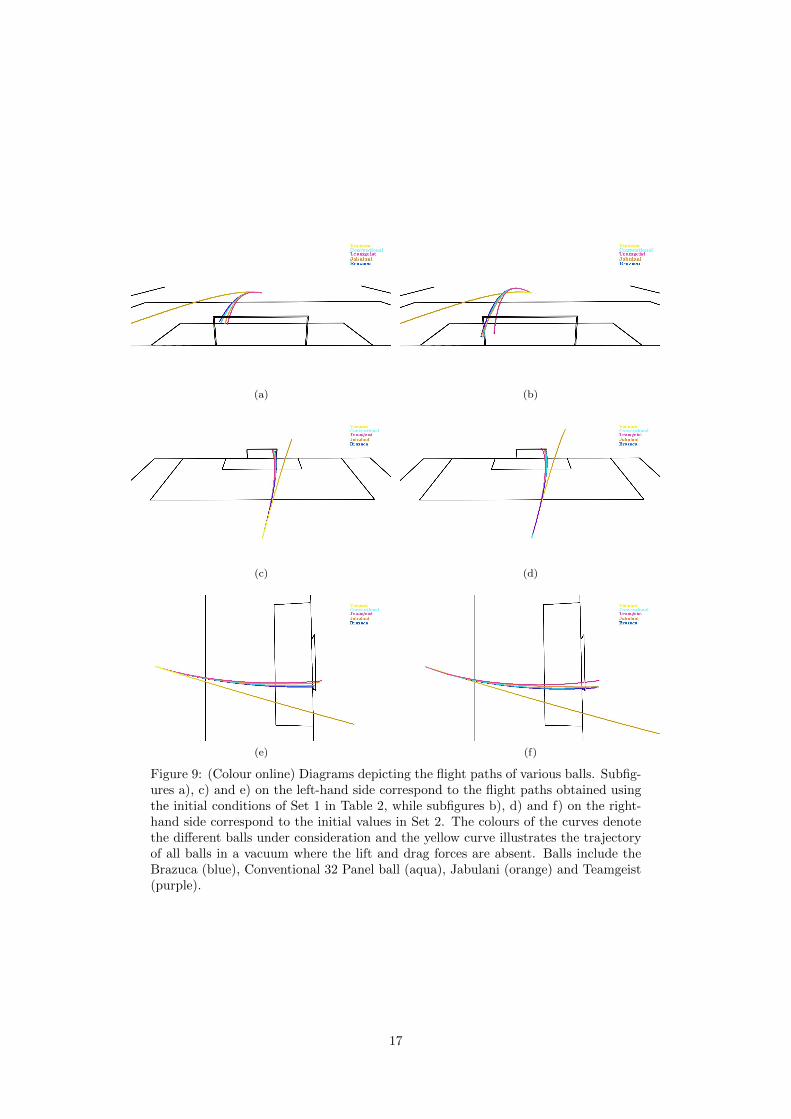
The illustrations of Figure 9 show this difference to have a significant impact, particularly onthe Jabulani’s trajectory. While the Set 1 initial speed of 34ms−1 is sufficiently fast that theboundary layer on all balls considered stays turbulent right until reaching the goal, this is not thecase with the initial speed of 27 ms−1 used in Set 2. Recall from Figure 5 that at approximately 24

12

ms−1 the Jabulani begins its transition from the turbulent to laminar regime, dramatically losinglift as the boundary layer moves away from the ball’s surface. This is particularly evident in theaforementioned figure where the Jabulani has encountered its transition, losing lift and crossingover the trajectory of the conventional 32-panel ball. This sensitivity of the lift coefficient toperturbation of initial speed within the speed range typical shots may arrive at the keeper, canfurther add to the inherent difficulty of the knuckleball effects the Jabulani experiences, discussedin Section 3. The angle of inclination is altered between the two sets of initial conditions in orderfor the ball to reach the goalmouth in a comparable position for both sets. Naturally, as playersare aiming for the goal, this reflects gameplay. Figure 9 also highlights the Teamgeist as the mostinteresting ball from an aerodynamics point of view. The long deep seams keep the flight in theturbulent regime, while its smooth panels keep the boundary layer intact at the highest speedsmaximising lift and associated curvature in the trajectory.

Figure 10 shows a comparison of the Brazuca and Jabulani with changing altitude. The initialconditions used for these simulations are Set 1 of Table 2. As discussed in Section 5 the capital cityin which the last two world cup finals were played was the venue with the highest elevation, whileboth world cups hosted matches played at sea level. The temperatures of 23◦C and 14◦C werechosen for the simulation as these were the pitchside temperatures at kickoff of the respective worldcup finals [41]. We readily observe that changing the altitude at which one plays can significantlyalter flight trajectories. At the time the ball went out of play (either for a goalkick or into the net),the difference in position for the Brazuca sea level kick and the one in Brasilia was 49.0 cm, whilethe corresponding difference for the Jabulani was notably more, at 82.0 cm. This relatively largevariation in the Jabulani’s behaviour derived solely from the different location at which the kickwas taken may well have further compounded previously discussed difficulties inherent to the ball.

While the altitude variation was significant, the difference in flight trajectories caused by thetemperature variation effect on air density is not as great, as can be readily deduced from Figure8. Figure 11 compares two kicks at the average minimum and maximum temperatures during thetournament months of June and July for both the Brazuca and Jabulani in the left hand and righthand columns respectively. At the time the ball went out of play (either for a goalkick or into thenet), the difference in position for the Brazuca at 12◦C and the Brazuca at 27◦C was 16.6 cm whilethe corresponding distance between the Jabulani kicked at 18◦C and 3◦C was 24.5 cm, both ofwhich are significantly less than the variation in trajectory seen resulting from changes in altitude.

8 Conclusions

Following a general summary of ball aerodynamics, we have developed a method for predicting thebehaviour of lift coefficients based on drag coefficient data, lift coefficient data as available and anunderstanding of the physics of the boundary layer. The drag coefficient data has also been fittedwith an improved functional form addressing high flow rate effects. This has been utilised to runaccurate simulations of various balls over typical match parameters.

While it was known that the high transition speed of the Jabulani caused knuckleball typeeffects at higher speeds, our boundary layer discussion indicates that this transition is likely tocoincide with a loss of lift. This has the potential to further compound other difficulties with theball, leading us to conclude that the players complaints in the 2010 world cup is supported by theavailable data and the present analysis.

We then considered the effect altitude and temperature has on flight trajectories, quantifyingthe difference in flight paths for the Brazuca and Jabulani at various altitudes and temperaturesexperienced at their respective world cups. We found that the variation observed in the Jabulani’sflight path in South Africa due to altitude variation was significant, perhaps further adding to thedifficulty the players experienced during the 2010 FIFA world cup.

While predicted lift coefficients from drag data coupled with an understanding of the boundarylayer provides an attractive framework within which we can produce accurate simulations, empiricallift data would be a natural extension. It would therefore be interesting to confront our theoreticalpredictions summarised in Equation 9 with experimentally measured lift coefficient values over arange of Reynolds numbers and spin parameters for a variety of balls, whether they be wind tunneldata or the results of trajectory analysis.

13

Acknowledgments

DBL thanks Jamie Seidel and the Advertiser newspaper for their interest and enthusiasm forexploring the physics of sports ball aerodynamics. The authors also thank Michels Warren fortheir permission to include the diagrams illustrating boundary layer separation in Section 2. Theirgenerosity is greatly appreciated. This research was supported by the School of Physical Sciencesat the University of Adelaide.

References

[1] http://www.physics.adelaide.edu.au/theory/staff/leinweber/Advertiser/

060610TurbulentTimes10jun06pgw02cropped.pdf

[2] http://www.physics.adelaide.edu.au/theory/staff/leinweber/Advertiser/

060527SurpriseAttack27may06pgw02cropped.pdf

[3] http://www.physics.adelaide.edu.au/theory/staff/leinweber/Advertiser/

051231SwingersDelight31dec05pgw02cropped.pdf

[4] http://www.physics.adelaide.edu.au/theory/staff/leinweber/Advertiser/

050910BehindTheSeams10sep05pgw02cropped.pdf

[5] http://www.physics.adelaide.edu.au/theory/staff/leinweber/Advertiser/

061202CricketInFullSwing02dec06pgw02cropped.pdf

[6] Mehta R D, Aerodynamics of sports balls. Ann. Rev. Fluid Mech. 17, 151-189, (1985).

[7] Mehta R D and Pallis J M, Sports ball aerodynamics: effects of velocity, spin and surfaceroughness. In Materials and Science in Sports, Proceedings of Symposium sponsored by TMS(The Minerals, Metals and Materials Society Warrendale, PA), (TMS press, Warrendale, PA),185-197, San Diego, (2001).

[8] Haake S J, Goodwill S R and Carre M J, A new measure of roughness for defining the aero-dynamic performance of sports balls. Proc. IMechE Vol.221 Part C:J. Mechanical EngineeringScience. 789-806, (2007).

[9] Alam F, Chowdhury H, Moria H and Brooy R L A Comparative Study of Golf Ball Aerody-namics. 17th Australasian Fluid Mechanics Conference, (2010).

[10] Nauro T and Mizota T, The Influence of Golf Ball Dimples on Aerodynamic Characteristics.Procedia Engineering 72 780-785, (2014).

[11] Mehta R D, An overview of cricket ball swing. Sports Engineering 8 181-192, (2005).

[12] Sayers A T and Hill A, Aerodynamics of a cricket ball. Journal of Wind Engineering andIndustrial Aerodynamics 79 169-182, (1999).

[13] Alam F, Ho H, Smith L, Subic A, Chowdhury H and Kumar A, A Study of Baseball andSoftball Aerodynamics. Procedia Engineering 34 86-91, (2012).

[14] Watts R.G, Sawyer E, Aerodynamics of a knuckleball, Am. J. Phys. Vol. 43, No. 11. November1975.

[15] Achenbach E, Experiments on the flow past spheres at very high Reynolds numbers. J. FluidMech. 54, 565-575,(1972).

[16] Achenbach E, The effects of surface roughness and tunnel blockage on the flow past spheres.J. Fluid Mech.,65, 113-125, (1974).

[17] http://espn.go.com/sports/soccer/news/_/id/6758280/least-1-billion-saw-part-

2010-world-cup-final

14

[18] http://www.fifa.com/mm/document/affederation/administration/01/60/80/10/

fifafinanzberichteinternet.pdf

[19] http://www.fifa.com/worldcup/news/y=2014/m=6/news=tv-viewing-breaks-records-

in-first-fifa-world-cup-matches-2378078.html

[20] http://www.fifa.com/tournaments/archive/worldcup/southafrica2010/highlights/

video/video=1246495/index.html

[21] Carre M J, Asai T, Akatsuka T and Haake S J, The curve kick of a football II:flight throughthe air. Sports Engineering 5, 193-200, (2002).

[22] Goff J E and Carre M J, Soccer ball lift coefficients via trajectory analysis. Eur. J. Phys. 31775-784, (2010).

[23] Goff J E, Kelley J, Hobson C M, Seo K, Asai T and Choppin S B, Creating drag and liftcurves from soccer trajectories. Eur. J. Phys. 38 044003, (2017).

[24] De Mestre N, The Mathematics of Projectiles in Sports (Cambridge: Cambridge UniversityPress) (1990).

[25] B. Robins, Mathematical Tracts, 1 & 2. J. Nourse, London, 1761

[26] Sengupta T K and Talla S B Robins-Magnus effect: A continuing saga Current Science. Vol.86(7), pp 1033-1036 (2004)

[27] Asai T, Seo K, Kobayashi O and Sakashita R, Fundamental aerodynamics of the soccer ball.Sports Engineering 10, 101-110, (2007).

[28] Thorsten K, J’org Franke, Wolfram F, Magnus effect on a rotating soccer ball at high Reynoldsnumbers, J. Wind Eng. Ind. Aerodyn. 124 (2014) 46-53.

[29] Takeshi Asai and Kazuya Seo: Aerodynamic drag of modern soccer balls, SpingerPlus, 2:171

[30] http://theconversation.com/hard-evidence-how-will-the-2014-world-cup-ball-

swerve-22985

[31] http://www.fifa.com/mm/document/footballdevelopment/refereeing/81/42/36/

log2013en_neutral.pdf

[32] Goff J E and Carre M J, Trajectory analysis of a soccer ball. Am. J. Phys., Vol. 77, No. 11,1020-1027, (2009).

[33] Bray K and Kerwin D G, Modelling the flight of a soccer ball in a direct free kick. Journal ofSports Sciences, 21, 75-85, (2003).

[34] Carre M J, Goodwill S R and Haake S J, Understanding the effect of seams on the aerody-namics of an association football. Proc. IMechE Vol.219 Part C:J. Mechanical EngineeringScience. 657-666, topview-Johannesburg-temp-comp.pdf(2005).

[35] Giordano N J and Nakanishi H, Computational Physics 2nd Edn (Englewood Cliffs, NJ:Prentice-Hall), (2006).

[36] Hong S, Chung C, Nakayama M and Asai T, Unsteady aerodynamic force on a knuckleball insoccer, Procedia Engineering 2 (2010) 24552460.

[37] Goff J E, Asai T and Hong S, A comparison of Jabulani and Brazuca non-spin aerodynamics,Proc IMechE Part P: J Sports Engineering and Teechnology 1-7, 2014.

[38] Levine S, Derivation of the ideal gas law, J. Chem. Educ., 1985, 62 (5), p 399 DOI:10.1021/ed062p399.1

[39] http://www.worldweatheronline.com/Brasilia-weather-averages/Distrito-

Federal/BR.aspx

15

[40] Press W.H, Teukolsky S.A, Vetterling W.T, Flannery B.P, Numerical Recipes in FORTRAN:The Art of Scientific Computing, Cambridge University Press, (1992).

[41] http://resources.fifa.com/mm/document/tournament/competition/02/40/47/25/eng_

64_0713_ger-arg_tacticalstartlist_neutral.pdf

16

(a) (b)

(c) (d)

(e) (f)

Figure 9: (Colour online) Diagrams depicting the flight paths of various balls. Subfig-ures a), c) and e) on the left-hand side correspond to the flight paths obtained usingthe initial conditions of Set 1 in Table 2, while subfigures b), d) and f) on the right-hand side correspond to the initial values in Set 2. The colours of the curves denotethe different balls under consideration and the yellow curve illustrates the trajectoryof all balls in a vacuum where the lift and drag forces are absent. Balls include theBrazuca (blue), Conventional 32 Panel ball (aqua), Jabulani (orange) and Teamgeist(purple).

17

(a) (b)

(c) (d)

(e) (f)

Figure 10: (Colour online) Diagrams comparing the flight paths of the Brazuca andJabulani over the range of altitudes encountered at their prospective world cups.Subfigures a), c) and e) on the left-hand side show comparisons with the Brazuca,while subfigures b), d) and f) on the right hand side depict Jabulani flight paths. Thetemperatures of 23◦C and 14◦C were the recorded temperatures at the respectivefinal’s kickoff time.

18

(a) (b)

(c) (d)

(e) (f)

Figure 11: (Colour online) Diagrams comparing the flight paths of the Brazuca andJabulani over the range of temperatures likely encountered at their prospective worldcups. Subfigures a), c) and e) on the left hand side show comparisons with theBrazuca, while subfigures b), d) and f) on the right hand side depict Jabulani flightpaths. The temperatures of 12◦C and 27◦C were the average minimum and maximumtemperatures during the tournament months of June and July in Brasılia, while 3◦Cand 18◦C were the average minimum and maximum temperatures during June andJuly in Johannesburg.

19