an alternative algorithm for empirical mode...

AN ALTERNATIVE ALGORITHM FOR EMPIRICAL MODE

DECOMPOSITION

LUAN LIN, YANG WANG, AND HAOMIN ZHOU

Abstract. The empirical mode decomposition (EMD) was a method pioneered by Huanget al [8] as an alternative technique to the traditional Fourier and wavelet techniques forstudying signals. It decomposes a signal into several components called intrinsic mode

functions (IMF), which have shown to admit better behaved instantaneous frequencies viaHilbert transforms. In this paper we propose an alternative algorithm for empirical modedecomposition (EMD). This approach yields similar results as the more traditional siftingalgorithm for EMD. In many cases the convergence can be rigorously proved.

1. Introduction

Signal and data analysis is an important and necessary part in both research and practical

applications. Understanding large data set is particularly important and challenging given

the explosion of data and numerous ways they are being collected today. While many

data sets are used to estimate parameters or to confirm certain models, finding hidden

information and structures is often a challenge in data and signal analysis. Unfortunately

for the latter we often encounter several difficulties: The data span is short; the data

represent a nonlinear process and is non-stationary; the essential information in the data is

often mingled together with noise or other irrelevant information.

Historically, Fourier spectral analysis has provided a general method for analyzing signals

and data. The term “spectrum” is synonymous with the Fourier transform of the data.

Another popular technique is the wavelet transform. These techniques are often effective,

but are known to have their limitations. To begin with, none of these techniques is data

adaptive. This can be a disadvantage in some applications. There are other limitations.

For example, the Fourier transform may not work well for non-stationary data or data from

Key words and phrases. Empirical mode decomposition (EMD), intrinsic mode function, Hilbert-Huangtransform, instantaneous frequency, sifting algorithm, low-pass filter.

The second and third authors are supported in part by the National Science Foundation, grants DMS-0811111, DMS-0410062 and DMS-0645266 respectively.

1

2 LUAN LIN, YANG WANG, AND HAOMIN ZHOU

nonlinear systems. It also does not offer spatial and temporal localization to be useful for

some applications in signal processing. The wavelet transform captures discontinuities very

successfully. But it too has many limitations; see [8] for a more detailed discussion.

The empirical mode decomposition (EMD) for data, which is a highly adaptive scheme

serving as a powerful complement to the Fourier and wavelet transforms, was proposed by

Norden Huang et al [8]. This study was motivated primarily by the need for an effective

way for analyzing the instantaneous frequency of signals, from which hidden information and

structures can often be brought to conspicuous view. The notion of instantaneous frequency

is not without controversies. It has not been accepted by all researchers in mathematics

and engineering, see e.g. [1]. Nevertheless this concept has proven to be useful in many

applications. Traditionally, instantaneous frequency of a signal is defined through its Hilbert

transform. Let X(t) be a function (a signal). The Hilbert transform X(t) is defined as

(1.1) XH(t) :=1

πPV

∫

R

X(s)

t − sds,

where PV is the principal value of the integral. Another way to understand the Hilbert

transform is from its Fourier transform. It is easy to show that (1.1) yields

XH(ξ) = −isign(ξ)X(ξ),

where sign(ξ) is the standard signum function taking the value +1 if ξ > 0, −1 if ξ < 0,

and 0 otherwise. Now write Z(t) := X(t) + iXH(t) = a(t)eiθ(t) where a(t) = |Z(t)|. The

instantaneous frequency at time t is now defined to be ω(t) := θ′(t).

The problem is that the instantaneous frequency obtained in this fashion is often mean-

ingless. A simple example is to take X(t) = cos(t) + b where b is a constant. We have

XH(t) = sin(t). For a = 0 the corresponding Z(t) = eit yields the perfect instanteneous

frequency ω(t) = 1. Ideally as we vary the constant b the instantaneous frequency should

remain the same. However, this is far from being true. For b = 1 we get Z(t) = 2 cos( t2 )ei t

2 ,

yielding ω(t) = 1/2. In fact by varying b one can obtain a continuum reading of instanta-

neous frequencies at any given t. Thus in this example for b 6= 0 the instantaneous frequency

obtained from the Hilbert transform is not meaningful.

The EMD was introduced in [8] to address this problem. In the EMD a data set is

decomposed into a finite, often small, number of components called Intrinsic Mode Functions

(IMF), which satisfy the following two conditions:

AN ALTERNATIVE ALGORITHM FOR EMPIRICAL MODE DECOMPOSITION 3

• The number of the extrema and the number of the zero crossings of an IMF must

be equal or differ at most by one.

• At any point of an IMF, the mean value of the envelopes defined by the local extrema

is zero.

Although it is by no means mathematically proven, IMFs do seem to admit in general better

behaved Hilbert transforms that often lead to meaningful readings for the instantaneous

frequency of the data. This process is known as the Hilbert-Huang transform (HHT). EMD

and HHT have found many successful applications in analyzing a very diverse range of data

sets in biological and medical sciences, geology, astronomy, engineering, and others; see

[2, 4, 8, 9, 13, 10]. Many of them cannot be fully captured easily by spectral or wavelet

techniques.

The original EMD is obtained through an algorithm called the sifting process. The local

maxima and minima in the process are respectively connected through cubic splines to

form the so-called upper and lower envelopes. The average of the two envelopes is then

subtracted from the original data. EMD is obtained after applying this process repeatedly.

The sifting algorithm is highly adaptive; it is also unstable. A small change in data can

often lead to different EMD. As powerful as EMD and HHT are in many applications, a

mathematical foundation is virtually nonexistent. Many fundamental mathematical issues

such as the convergence of the sifting algorithm, the orthogonality of IMFs and others

have never been established. The difficulty is partly due to the highly adaptive nature of

the sifting algorithm as well as the ad hoc nature of using cubic splines. In [2] the cubic

splines were replaced by B-splines, which gives an alternative way for EMD. But again this

modification does not resolve those mathematical issues. Overall, building a mathematical

foundation remains a big challenge in the study of EMD and HHT. Norden Huang, the

principal author of [8], has repeatedly called for help from mathematicians who have been

working in the area.

This paper is an attempt to address the aforementioned mathematical issues, and to lay

down a mathematical framework for an alternative approach to EMD. Given the difficulty

encountered from relying on cubic splines or B-splines, our alternative algorithm calls for

replacing the mean of the envelopes by certain “moving average” in the sifting algorithm.


The moving average can be adaptive in the sense that it is data dependent. We establish

rigorous mathematical criteria for convergence under certain conditions.

It should be pointed out that as with the B-spline EMD, our new approach to EMD may

or may not lead to similar decompositions as the traditional EMD. It is not our intention to

claim that this alternative algorithm for EMD is superior to the traditional EMD. Rather,

our intention is to present a different approach that can serve as a complement to it,

with which some rigorous mathematical properties can be proved. An added advantage

is that this alternative approach can readily be extended to higher dimensions. We hope

that our attempt will encourage others to do likewise in our combined effort to lay out a

comprehensive mathematical foundation for EMD and the Hilbert-Huang transform.

2. An Alternative Algorithm for EMD

The essence of EMD is to decompose a signal into intrinsic mode functions, from which the

instantaneous frequencies can be analyzed using HHT. Before discussing our own approach

we first briefly describe the sifting algorithm for the traditional EMD. Let X(t) be a function

representing a signal, where t ∈ R or t ∈ Z. Let {tj} be the local maxima for X(t). The

cubic spline EU (t) connecting the points {(tj ,X(tj))} is referred to as the upper envelope

of X. Similarly, with the local minima {sj} of X we also have the lower envelope EL(t) of

X. Now define the operator S by

(2.1) S(X) = X − 1

2(EU + EL).

In the sifting algorithm, the first IMF in the EMD is given by

I1 = limn→∞

Sn(X),

where Sn means applying the operator S successively n times. The limit is taken so that

repetitively applying S will no longer change the remaining signal. This implies that the

resulting I1 is an IMF, which has zero mean everywhere. Subsequent IMF’s in the EMD

are obtained recursively via

(2.2) Ik = limn→∞

Sn(X − I1 − · · · − Ik−1).


The process stops when Y = X − I1 − · · · − Im has at most one local maximum or local

minimum. This function Y (t) denotes the trend of X(t). The EMD is now complete with

(2.3) X(t) =

m∑

j=1

Ij(t) + Y (t).

One of the main unresolved questions mentioned earlier is the convergence of Sn(X) in

general. Even though in practice we stop the iteration once some stopping criterion is met

(and the stopping criterion rarely calls for high precision), it is still important to know

whether such criterion will ever be met. Interestingly, although there is no mathematical

proof for the convergence, there have been no examples in which the sifting algorithm fails

to stop.

We should point out that the sifting process is highly adaptive and nonlinear. At different

stages the sifting operators are different. Thus the notation Sn is in fact an abuse of

notation. However, given the is no confusion we shall adopt it anyway because of its

simplicity.

Here we propose an alternative algorithm for EMD. Instead of using the envelopes gen-

erated by splines we use a “moving average” to replace the mean of the envelopes. The

essence of the sifting algorithm remains. Let L be an operator such that L(X)(t) represents

some moving average of X. Now define

(2.4) T (X) = X − L(X).

The IMF’s are now obtained precisely via the same sifting algorithm (2.2) for obtaining

the traditional IMF’s, where the operator S is now replaced by T . Note again we abuse

the notation here because at diferet steps the operator L are different. Thus, The first

IMF in our EMD is given by I1 = limn→∞ T n(X), where T n means applying operator Tsuccessively n time to X and subsequently Ik = limn→∞ T n(X − I1 − · · · − Ik−1). Again

the process stops when Y = X − I1 − · · · − Im has at most one local maximum or local

minimum.

The critical question is how do we choose the moving average operator L(X) to replace

the mean of the envelopes. Ideally this choice should be data adaptive, easy to implement

and analyze, and the sifting algorithm should converge. The simplest choice for the moving

average is an adaptive local weighted average.


Since in applications the data are discrete and finite, we shall focus first on X(t) being a

discrete-time signal, X = X(n) where n ∈ Z. We consider the moving average Y = L(X)

given by Y (n) =∑m

j=−m aj(n)X(n + j), where m = m(n). a(n) = (aj(n))mj=−m is called

the mask (or filter coefficients) for L at n. We say L has uniform mask if a(n) = a are

independent of n, and use La to denote this operator. In other words, La(X) = Y has

Y (n) =∑m

j=−m ajX(n + j).

When EMD is applied to stationary data it makes sense to use a uniform mask (chosen

adaptively) for the operator L in the process of extracting each IMF. An advantage of

uniform mask is that in this setting we can establish rigorous convergence criteria, which we

prove below. For many nonstationary data, however, a uniform mask may not work as well.

One may need to choose L with nonuniform mask. We shall discuss these later. One of the

major issues is that with nonuniform mask the convergence of the sifting algorithm is harder

to establish mathmetically. This is perhaps why we have focused more on the uniform mask

case. However, there is some encouraging recent development in this direction. Convergence

criteria for a broad class of L with nonuniform mask have been established in an ongoing

work by Huang and Yang [7]. Our numerical examples will include both cases.

To study finite data it is common that we extend them to infinite data via some form of

periodic extension. So without loss much generality we may assume X = X(n) is periodic,

i.e. there exists an N > 0 such that X(n+N) = X(n) for all n ∈ Z. The following theorem

establishes the convergence of the sifting algorithm in the uniform mask setting.

Theorem 2.1. Let a = (aj)mj=−m and T (X) = X−La(X). Denote a(ξ) =

∑mj=−m aje

2πijξ.

(i) Let N > 2m. Then T n(X) converges for all N -periodic X(n) if and only if for all

ξ ∈ 1N

Z we have either a(ξ) = 0 or |1 − a(ξ)| < 1.

(ii) T n(X) converges for all periodic X(n) if and only if for all ξ ∈ Q we have either

a(ξ) = 0 or |1 − a(ξ)| < 1.

Proof. We first prove (i). Since for every N -periodic X the function Y = T (X) is also

N -periodic, the convergence of Yn := T n(X) is equivalent to the convergence of

yn := [Yn(0), Yn(1), . . . , Yn(N − 1)]T .

Now we extend a to (aj : −m ≤ j ≤ N − m − 1) such that aj = 0 for j > m. Define the

N ×N matrix M = [cij ]N−1i,j=0 by cij = ak where k is the unique integer −m ≤ k ≤ N −m−1


such that k ≡ i + j (mod N). We have

yn = (IN − M)nx

where x = [X(0),X(1), . . . ,X(N − 1)]T . Thus yn converges for all x ∈ RN if and only if

the eigenvalues λ of I −M have either λ = 1 or |λ| < 1 and the dimension of the eigenspace

for λ = 1 equals the multiplicity of the eigenvalue 1. Note that M is a cyclic matrix whose

eigenvalues are well known to be precisely a(j/N), j = 0, 1, . . . ,N −1, counting multiplicity

(these values may not be distinct), with corresponding eigenvectors

vj = [1, ωjN , ω2j

N , . . . , ω(N−1)jN ]T

where ωN = e2πiN . The eigenvalues of I − M are thus 1 − a(j/N), j = 0, 1, . . . ,N − 1,

counting multiplicity. The vectors {vj} are linearly independent because the N ×N matrix

[v0,v1, · · · ,vN−1] is a Vandermonde matrix with distinct columns. This implies that the

dimension of the eigenspace for the eigenvalue 1 equals its multiplicity. Hence yn converges

for all x ∈ RN if and only if for all j = 0, 1, . . . ,N − 1 we have either a(j/N) = 0 or

|1 − a(j/N)| < 1. Note that a(ξ) = a(ξ + 1). Part (i) of the theorem now follows.

Part (ii) is essentially a corollary of part (i). First, observe that if X is N -periodic that

if is also kN -periodic. So we may without loss of generality consider the convergence for all

periodic X with period N > 2m. Part (ii) now follows from part (i) as Q =⋃

N>2m1N

Z.

Corollary 2.2. Let a = (aj)mj=−m and T (X) = X−La(X). Assume that for an N -periodic

X(n) we have limn→∞ T n(X) = Y , where N > 2m. Then

(2.5) Y =∑

k∈Γ

ckEk,

where Γ = {0 ≤ k < N : a(k/N) = 0}, Ek is given by Ek(n) = e2πikn

N and

ck =1

N

N−1∑

j=0

X(j)e−2πikj

N .

Proof. Let x = [X(0),X(1), . . . ,X(N − 1)]T and y = [Y (0), Y (1), . . . , Y (N − 1)]T . Then

y = limn→∞ Mnx, where M is defined in the proof of Theorem 2.1. The vectors vj defined

in the proof of Theorem 2.1 are eigenvectors for the eigenvalues 1 − a(j/N), respectively.

They also form an orthogonal basis for CN . Write

x =N−1∑

k=0

ckvk


where ck = 1N

∑N−1j=0 X(j)e−

2πikj

N . Then

Mnx =

N−1∑

k=0

ck(1 − a(k/N))nvk.

This yields y =∑

k∈Γ ckvk should Mnx converges. The corollary now follows.

It is worth noting that many high pass filters also satisfy the convergence conditions. But

they are not suitable for obtaining the moving averages of signals and we do not consider

them in this study.

In practical applications we often choose to make the masks symmetric, i.e. aj(n) =

a−j(n) for all j and n. For a symmetric mask a we have a(ξ) ∈ R. In this case, it is easy

to see that a has the property that for all ξ ∈ Q we have either a(ξ) = 0 or |1 − a(ξ)| < 1

is equivalent to the property that 0 ≤ a(ξ) < 2 for all ξ ∈ Q, which is in turn equivalent to

0 ≤ a(ξ) ≤ 2 for all ξ ∈ R with a(ξ) 6= 2 for ξ ∈ Q.

Proposition 2.3. Let a = (aj)mj=−m be a symmetric mask. Then 0 ≤ a(ξ) ≤ 2 for all ξ ∈ R

is equivalent to a(ξ) = |b(ξ)|2 for some mask b = (bj)mj=0 with |b(ξ)| ≤

√2.

Proof. The fact that a(ξ) = |b(ξ)|2 for some mask b follows directly from Fejer-Riesz

Theorem since a(ξ) ≥ 0 is a nonnegative trigonometric polynomial. Obviously we must have

|b(ξ)| ≤√

2. Finally we can always choose in the form of b = (bj)lj=0 because translating

the mask does not change |b(ξ)|2. Now we can choose l = m because the support of a is

from −m to m.

A simple class of L with uniform mask is the double averaging filter with mask am where

am is given by am(ξ) = |bm(ξ)|2, with bm = (bj)mj=0, bj = 1

m+1 . When m is an odd number,

this is equivalent to averaging over the neighborhood of radius m twice. am = (aj)mj=−m has

the explicit expression aj = (m+1−j)/(m+1)2. It is clear that the double averaging masks

satisfy the condition 0 ≤ a(ξ) ≤ 1 so convergence of the sifting algorithm with T = I − La

is assured. Furthermore, the zeros of them are known: am(ξ) = 0 if and only if ξ = km+1 ,

1 ≤ k ≤ m + 1.

An adaptive version of the double averaging filter seem to work well numerically. In this

version, the moving average operator L has mask am at n with m = m(n). By varying

m(n) according to the local density of the local extrema this approach seems to work well


for nonstationary data in numerical experiment. The convergence of the sifting algorithm,

however, has not been established yet.

In the continuous setting the moving average can be similarly defined through an integral

operator

(2.6) L(X)(t) =

∫

R

k(s, t)X(s)ds.

The equivalence of uniform mask in the continuous setting is to set k(s, t) = g(s − t) for

some g. For periodic functions the convergence with uniform kernel is easily analyzed by

considering the Fourier transform of the kernel. Also, one attractive feature of this alterna-

tive approach to EMD is its easy extension to higher dimensions. The entire machinery can

readily be adopted for use on higher dimensional data. Such study will be presented in a

future paper. A far more challenging mathematical problem is to analyze the convergence

of T n(X) for general X ∈ l∞. This question is considered by Wang and Z. Zhou in [14].

3. Implementation of the Alternative Algorithm for EMD

We have primarily focused on using the double averaging filter to perform this alternative

approach of EMD. This is partly because of its simplicity as well as its effectiveness in our

experiments. For effective sifting we need to choose both the right window size for the

double averaging mask and the right stopping criteria.

In our approach we choose the window size of our filter primarily according to the fre-

quency of oscillations in the signal, which is very much related to how the envelopes are

obtained in [8]. Let N be the sample size of our data X(t), and let k be the number of local

maxima and minima in the data. The simplest way to choose the window size is

(3.1) m =

⌊αN

k

⌋

where α can be adjusted. For most of our numerical experiments we choose α = 2. This

setting works very well for stationary X(t); even for some nonstationary ones it seems to

work well, see the examples in the next section. We have also found that the algorithm is

rather robust with respect to small perturbations of the parameter α.

For nonstationary data, especially extremely nonstationary data, it will be wise to use

a more adaptive moving average with nonuniform mask. More sophisticated method for

choosing the mask will be needed. It is rather natural to choose a moving average operator


whose mask at time t depends on the local density of the extrema. We shall describe in

detail how such nonuniform masks were chosen in [7] in one of the examples later. The

convergence of sifting algorithm with nonuniform mask in the continuous time setting is

established in [7] for certain class of signals. In the discrete time setting the convergence

appears more difficult to prove. A more comprehensive study on this is an ongoing project.

An important part of EMD is the stopping criteria for the sifting algorithm. For this we

employ the same standard deviation criteria as in [8]. Let Ik,n(t) = T nk (X(t)− I1(t)− · · · −

Ik−1(t)). Define

(3.2) SD =

∑N−1t=0

∣∣Ik,n(t) − Tk,n−1(t)∣∣2

∑N−1t=0

∣∣Tk,n−1(t)∣∣2 .

We stop the iteration when SD reaches certain threshold. The smaller SD is the more sifting

we do. There is a clear tradeoff here. With a small SD more IMFs will be obtained, some

of them may not be useful to lead us to more insight. With a larger SD one may not be

able to obtain satisfactory separations. This is an area where further study will be needed.

In our numerical experiments we have used SD ranging from 0.001 to 0.2. For one of the

examples in this paper, a small SD was needed to separate sin(2t) and sin(4t).

4. Numerical Experiments

In this section we demonstrate the performance of the proposed new apporach to EMD

through a series of examples involving a wide variety of data. We examine the IMF’s and

their instantenous frequencies.

In all our numerical experiments we determine the window size m in each decomposition

as in (3.1) with α = 2. Unless otherwise specified we use SD = 0.2 for our stopping criterion.

Note that by lowering the value SD we can achieve better separations in general. However,

this will often yield more IMF’s, especially when the data have noise. It should be noted

that in different illustrations the scales often vary to better illustrate each IMF.

Example 1. We first test our EMD on a standard test functions, where the test functions

are combinations of two sinusoidal functions. Figure 4 left is given by

f(t) = sin(t) + sin(4t).


0 1 2 3 4 5 6 7−2

−1.5

−1

−0.5

0

0.5

1

1.5

2

0 1 2 3 4 5 6 7−2

−1.5

−1

−0.5

0

0.5

1

1.5

2

0 1 2 3 4 5 6 7−2

−1.5

−1

−0.5

0

0.5

1

1.5

2

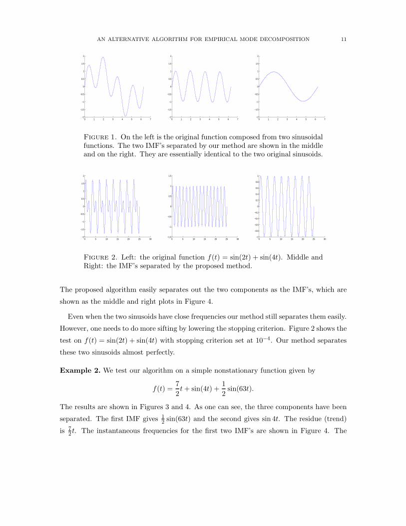
Figure 1. On the left is the original function composed from two sinusoidalfunctions. The two IMF’s separated by our method are shown in the middleand on the right. They are essentially identical to the two original sinusoids.

0 5 10 15 20 25 30−2

−1.5

−1

−0.5

0

0.5

1

1.5

2

0 5 10 15 20 25 30−1.5

−1

−0.5

0

0.5

1

1.5

0 5 10 15 20 25 30−1

−0.8

−0.6

−0.4

−0.2

0

0.2

0.4

0.6

0.8

1

Figure 2. Left: the original function f(t) = sin(2t) + sin(4t). Middle andRight: the IMF’s separated by the proposed method.

The proposed algorithm easily separates out the two components as the IMF’s, which are

shown as the middle and right plots in Figure 4.

Even when the two sinusoids have close frequencies our method still separates them easily.

However, one needs to do more sifting by lowering the stopping criterion. Figure 2 shows the

test on f(t) = sin(2t) + sin(4t) with stopping criterion set at 10−4. Our method separates

these two sinusoids almost perfectly.

Example 2. We test our algorithm on a simple nonstationary function given by

f(t) =7

2t + sin(4t) +

1

2sin(63t).

The results are shown in Figures 3 and 4. As one can see, the three components have been

separated. The first IMF gives 12 sin(63t) and the second gives sin 4t. The residue (trend)

is 72t. The instantaneous frequencies for the first two IMF’s are shown in Figure 4. The


0 1 2 3 4 5 60

5

10

15

20

25

0 1 2 3 4 5 6−0.5

−0.4

−0.3

−0.2

−0.1

0

0.1

0.2

0.3

0.4

0.5

0 1 2 3 4 5 6−1

−0.8

−0.6

−0.4

−0.2

0

0.2

0.4

0.6

0.8

1

Figure 3. Left: A nonstationary function. The middle and right plots arethe first two IMF’s separated by the proposed alternative EMD algorithm.

0 1 2 3 4 5 60

5

10

15

20

25

0 1 2 3 4 5 60

10

20

30

40

50

60

70

80

90

100

0 1 2 3 4 5 60

1

2

3

4

5

6

7

8

9

10

Figure 4. Left: the third IMF (trend) of the signal shown on the left inFigure 3. The middle and right pictures show the instantaneous frequenciesfor the second (middle) and third (right) IMF’s shown in Figure 3.

instantaneous frequency function for the IMF’s lie around 63 and 4 respectively, as they are

supposed to be.

Example 3. We test our algorithm on a frequency modulated signal with additive noise.

Here the signal is given by

f(t) = 2 sin(2t + 0.65 sin(t2)) + 5 sin(9.125t + 0.037t2) + ǫ(t),

where ǫ(t) is a spatially uniformly distributed random variable in [−0.5, 0.5]. The IMF’s are

shown in Figure 5. The first two IMF’s correspond to noise. The last IMF is the residual

trend. The most relevant IMF’s are the 4th and the 5th, which correspond to the two FM

components. Their instantaneous frequencies are shown in Figure 6.


0 1 2 3 4 5 6−8

−6

−4

−2

0

2

4

6

8

0 1 2 3 4 5 6−0.5

−0.4

−0.3

−0.2

−0.1

0

0.1

0.2

0.3

0.4

0.5

0 1 2 3 4 5 6−0.5

−0.4

−0.3

−0.2

−0.1

0

0.1

0.2

0.3

0.4

0.5

0 1 2 3 4 5 6−6

−4

−2

0

2

4

6

0 1 2 3 4 5 6−6

−4

−2

0

2

4

6

0 1 2 3 4 5 6−6

−4

−2

0

2

4

6

Figure 5. Top left: the original function of two FM signals with additivenoise. The others are the IMF’s separated by our method.

0 1 2 3 4 5 60

5

10

15

0 1 2 3 4 5 60

0.5

1

1.5

2

2.5

3

3.5

4

4.5

5

Figure 6. The instantaneous frequencies of the 4th and the 5th IMF’sshown in Figure 5 respectively.

Example 4. In this example we test the impact of noise. This is a rather challenging case

given the amount of noise and the proximity of the two frequencies. Let

f(t) = sin(2t) + 2 sin(4t) + η(t),

where η(t) is an i.i.d Gaussian random noise of distribution N(0, 3). The signal-to-noise

ratio is −5.6 dB. With the stopping criterion set as 10−4, our method yields 11 IMF’s. The

first 9 components essentially correspond to noise. Figure 7 plots the original signal and

the last three IMF’s. We omit the first eight IMF’s since they mainly correspond to the


0 5 10 15 20 25 30 35−15

−10

−5

0

5

10

15

0 5 10 15 20 25 30 35−0.8

−0.6

−0.4

−0.2

0

0.2

0.4

0.6

0.8

1

0 5 10 15 20 25 30 35−5

−4

−3

−2

−1

0

1

2

3

4

5

0 5 10 15 20 25 30 35−2

−1.5

−1

−0.5

0

0.5

1

1.5

2

Figure 7. Left: The original signal f(t) = sin(2t) + 2 sin(4t) + η(t) whereη(t) is an i.i.d. Gaussian noise with distribution N(0, 3). The other threeplots show the 9th, 10th and 11th IMF’s, respectively.

noise. It is quite remarkable that the last two components actually closely recover the two

sinusoidal components in the original signal. We have also tested for uniform noise from -6

to 6. The noise-to-signal ratio is 6.8 dB. The result is quite similar.

Example 5. This example demonstrates how nonuniform mask can be used to treat a highly

nonstationary signal, courtesy of the authors of [7]. Let f(t) = cos(4πλ(t)t) + 2 sin(4πt)

where λ(t) is given by λ(t) = 4 + 32t for 0 ≤ t ≤ 0.5 and its symmetric reflection λ(t) =

λ(1 − t) for 0.5 ≤ t ≤ 1. As before we work with the discretized version of f(t) with

x(k) = f(k/N). To perform EMD using nonuniform double average filter mask one needs

to find a good mechanism for specifying the length of the mask at a given k. This is done

as follows in [7]: Let nj be the local extrema of the discretized x(k). The mask length at

k = nj is

w(nj) =2N

nj+2 − nj−2.

Now connect the points (nj , w(nj)) using a cubic spline. The mask length w(k) for any

other k is given by the interpolated value using the spline. Using this non-uniform mask


-2.96e+000

3.00e+000

-2.07e+000

2.01e+000

-5.58e-001

7.09e-001

-9.99e-001

9.81e-001-2.98e+000

3.00e+000

-2.05e+000

2.02e+000

-1.08e+000

1.05e+000

Figure 8. The left figure shows EMD using uniform mask, where the orig-inal is at the top and the other three are the IMF’s. The right figure showsEMD using the aforementioned non-uniform mask, with a virtually perfectdecomposition.

the EMD yields essentially a perfect decomposition with two IMF’s, see the right figure in

Figure 8. In comparison, the EMD using uniform mask is given on the left of Figure 8.

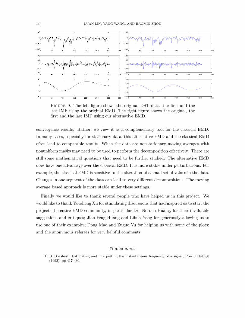
Example 6. We compare the traditional EMD with this alternative EMD using a couple

of real world data. Figure 9 is a partial side-by-side comparison of the two algorithms on

DST data. The traditional EMD yields 5 IMF’s while our method yields 7 IMF’s. Figures

9 and 11 compare the first 11 IMF’s of the rainfall data using our alternative EMD and the

original EMD, respectively. As one can see the similarities are unmistaken.

5. Conclusion

In this paper we have provided an alternative algorithm for the empirical mode decom-

position (EMD). This alternative approach replaces the mean of the spline-based envelopes

in the original sifting algorithm by an adaptively chosen moving average.

One of the goals of this alternative algorithm is to address the concern that the classical

EMD is hard to rigorously analyze mathematically due to the lack of analytical characteri-

zation of the cubic spline envelopes. The use of a moving average allows in many cases for

a more rigorous mathematical analysis of this proposed alternative EMD.

We would like to emphasize once again that it is not our intention to claim that this

alternative EMD is superior to the classical EMD simply because it allows us to prove some


0 50 100 150 200 250 300 350−200

−100

0

100

0 50 100 150 200 250 300 350−100

−50

0

50

100

0 50 100 150 200 250 300 350−20

−10

0

10

20

Figure 9. The left figure shows the original DST data, the first and thelast IMF using the original EMD. The right figure shows the original, thefirst and the last IMF using our alternative EMD.

convergence results. Rather, we view it as a complementary tool for the classical EMD.

In many cases, especially for stationary data, this alternative EMD and the classical EMD

often lead to comparable results. When the data are nonstationary moving averages with

nonuniform masks may need to be used to perform the decomposition effectively. There are

still some mathematical questions that need to be further studied. The alternative EMD

does have one advantage over the classical EMD: It is more stable under perturbations. For

example, the classical EMD is sensitive to the alteration of a small set of values in the data.

Changes in one segment of the data can lead to very different decompositions. The moving

average based approach is more stable under these settings.

Finally we would like to thank several people who have helped us in this project. We

would like to thank Yuesheng Xu for stimulating discussions that had inspired us to start the

project; the entire EMD community, in particular Dr. Norden Huang, for their invaluable

suggestions and critiques; Jian-Feng Huang and Lihua Yang for generously allowing us to

use one of their examples; Dong Mao and Zuguo Yu for helping us with some of the plots;

and the anonymous referees for very helpful comments.

References

[1] B. Boashash, Estimating and interpreting the instantaneous frequency of a signal, Proc. IEEE 80(1992), pp 417-430.


0 2000 4000 6000 8000 10000 12000 14000 16000 180000

100

200

0 2000 4000 6000 8000 10000 12000 14000 16000 18000−100

0

100

0 2000 4000 6000 8000 10000 12000 14000 16000 18000−20

0

20

0 2000 4000 6000 8000 10000 12000 14000 16000 18000−20

0

20

0 2000 4000 6000 8000 10000 12000 14000 16000 18000−10

0

10

0 2000 4000 6000 8000 10000 12000 14000 16000 18000−5

0

5

0 2000 4000 6000 8000 10000 12000 14000 16000 18000−5

0

5

0 2000 4000 6000 8000 10000 12000 14000 16000 18000−5

0

5

0 2000 4000 6000 8000 10000 12000 14000 16000 18000−5

0

5

0 2000 4000 6000 8000 10000 12000 14000 16000 18000−0.5

0

0.5

Figure 10. First 11 IMFs of the rainfall data using the alternative EMD

[2] Q. Chen, N. Huang, S. Riemenschneider and Y. Xu, B-spline approach for empirical mode decom-position, preprint.

[3] L. Cohen, Time-Frequency Analysis. Englewood Cliffs, NJ, Prentice Hall (1995).[4] J. C. Echeverria, J. A. Crowe, M. S. Woolfson and B. R. Hayes-Gill, Application of empirical mode

decomposition to heart rate variability analysis, Medical and Biological Engineering and Computing39 (2001), pp 471-479.

[5] P. Flandrin, G. Rilling, and P. Gonalves, Empirical mode decomposition as a filter bank, IEEE

Signal Processing Lett. 11 (2004), pp 112-114.


Figure 11. First 11 IMFs of the rainfall data using the original EMD

[6] P. Flandrin, P. Gonalves and G. Rilling, EMD equivalent filter banks, from interpretation to appli-cations, in Hilbert-Huang Transform : Introduction and Applications, N. E. Huang and S. Shen Ed,World Scientific, Singapore (2005), pp 67–87.

[7] J.-F. Huang and L. Yang, Empirical mode decomposition based on locally adaptive filters, preprint.[8] N. Huang et al, The empirical mode decomposition and the Hilbert spectrum for nonlinear nonsta-

tionary time series analysis, Proceedings of Royal Society of London A 454 (1998), pp 903-995.[9] N. Huang, Z. Shen and S. Long, A new view of nonlinear water waves: the Hilbert spectrum, Annu.

Rev. Fluid Mech. 31 (1999), pp 417-457.[10] B. Liu, S. Riemenschneider and Y. Xu, Gearbox fault diagnosis using emperical mode decomposition

and hilbert spectrum, preprint.


[11] S. Mallat, A Wavelet Tour of Signal Processing. London, Academic Press (1998).[12] R. Meeson, HHT Sifting and Adaptive Filtering, in Hilbert-Huang Transform : Introduction and

Applications, N. E. Huang and S. Shen Ed, World Scientific, Singapore (2005), pp 75–105.[13] D. Pines and L. Salvino, Health monitoring of one dimensional structures using empirical mode

decomposition and the Hilbert-Huang Transform, Proceedings of SPIE 4701(2002), pp 127-143.[14] Y. Wang and Z. Zhou, On the convergence of EMD in l

∞, preprint.[15] Z. Wu and N. E. Huang, A study of the characteristics of white noise using the empirical mode

decomposition method, Proc. Roy. Soc. London 460A (2004), pp 1597–1611.[16] Z. Wu and N. E. Huang, Statistical significant test of intrinsic mode functions. in Hilbert-Huang

Transform : Introduction and Applications, N. E. Huang and S. Shen Ed, World Scientific, Singapore(2005), pp 125-148.

[17] Z. Wu and N. E. Huang, Ensemble empirical mode decomposition: a noise-assisted data analysismethod, Center for Ocean-Land-Atmosphere Studies, Technical Report No. 193 (2005), downloadfrom http://www.iges.org/pubs/tech.html

School of Mathematics, Georgia Institute of Technology, Atlanta, Georgia 30332-0160,

USA.

E-mail address: [email protected]

Department of Mathematics, Michigan State University, East Lansing, MI 48824-1027, USA.


School of Mathematics, Georgia Institute of Technology, Atlanta, Georgia 30332-0160,

USA.


an alternative algorithm for empirical mode...

Documents