An Alternative to the Feltham-Ohlson ValuationFramework: Using q-Theoretic Income to Predict Firm

Value

Miles B. GietzmannCass Business School

City University

Adam OstaszewskiDept. of Mathematics

London School of Economics

May 2003, altgo-conf.tex

Abstract

In this model we provide a theoretical justi¯cation for why the functional relationshipbetween earnings and value will be non linear. Moreover in our stylized model we derivea closed form for the relationship and show why earnings response coe±cients are lowerfor ¯rms that are contracting or expanding relative to those ¯rms that are maintaininga steady investment strategy. We extend earlier research which posits a simple convexrelationship based upon ¯xed abandonment values and also generalize research which usesreal options valuation models based upon the assumption that ¯rms only ever exerciseone real investment option and then are committed to that strategy ad in¯nitum. Inparticular, since in some empirical settings the special case of `¯xed' abandonment willnot apply, we show how the form of convexity changes. Secondly, in our model ¯rmsare allowed to dynamically change investment strategies, for instance expanding in oneperiod followed by contraction in the subsequent period. Given an objective of derivingcomparative statics results for earnings response coe±cients, our dynamic model is ableto capture more accurately real investment behavior than a model in which ¯rms onlyever decide to expand or contract once. Our model provides both an alternative rationalefor accounting measures having information content and an alternative framework for theempirical speci¯cation of tests of `accounting value relevance' based upon ¯nite mixture(regime-switching) distributions. Our model shows how one can view equity value ascomprising opening cash, q-revalued opening stock, current q-income and future q-income.

We are grateful for comments from Nick Bingham, Graham Brightwell, Patricia De-chow, Mike Kirschenheiter, Russ Lundholm, John O'Hanlon, and from seminar partici-pants at the University of Lancaster, EIASM Madrid Economics and Accounting work-shop, and at King's College London.

1

1 INTRODUCTION

In this section we discuss the established Feltham-Ohlson (FO) valuation model and brie°yreview the main ¯ndings and some related research. We argue that, since the FO approachhas no transparent role for management, the approach excludes consideration of important realoptions that typically arise empirically when investment decisions are undertaken. In addition,we present a simple example that shows that the traditional residual income number is not theonly accounting measure which admits valuation equivalence to the discounted dividend stream.Another well-known criticism, following Peasnell (1982), of the clean surplus class of models,such as FO, is that the models do not give rise to any structural implications for the applicationof accounting rules. That is, it may be hard to argue that the models present a justi¯cation foraccrual accounting when there is little evidence of the need for accrual adjustments. Exploitingthis equivalence type result we show that a di®erent form of residual income valuation doesgive rise to a reasonably tractable method for analyzing optimal investment decisions anddevelops an approach to go beyond the general equivalence result and identify a restricted setof accounting measures that meet a certain `axiomatic' property, as follows. When consideringcandidate earnings numbers with the intention of predicting ¯rm value, we require that asthe chosen earnings number increases, this rationally results in higher estimates of future ¯rmvalue. We thus propose that this simple monotonicity property should be satis¯ed by candidateearnings measures, on the grounds that investors will question any measurement methods of anearnings number for which current higher earnings, can mean lower ¯rm value in the future.

Initially, one may suspect that satisfaction of this seemingly quite mild axiomatic conditionwill not be particularly discriminating and that many earnings measures will satisfy the axiom.However, interestingly, we ¯nd that the established earning measure used in the literature(residual income) fails to satisfy the axiom and show how an alternative income measure basedupon the established q-theory of income does satisfy the axiom. Clearly, with one simple axiomwe cannot provide a way to discriminate between all possible earnings measures. However, wesuggest that unlike the FO approach which provides no discrimination, our analytical approachis amenable to testing the satisfaction of additional well-speci¯ed axiomatic requirements andso o®ers the ability to re¯ne the number of candidate earnings numbers that satisfy a chosenset of axioms1.

In addition to providing a theoretical means to discriminate between alternative earningsmeasures, our approach also contributes to empirical issues. In particular, since our approach isbased upon multi-period optimization, we are able to derive comparative statics results whichexplain in a constructive way, why for instance, earnings response is non linear. In particularwe show why for ¯rms that are expanding aggressively, the earnings response coe±cient may bequite low. Since our model is based upon optimizing behaviour we believe we may o®er a supe-rior explanation for the role of earnings in estimating future value in such settings than thoseresearchers who simply conclude that a low earnings response coe±cient may be interpreted

1We believe this to be of some importance at this time, given the active debate concerning the overalldesirability of comprehensive and other earnings measures.

2

as evidence of the lack of usefulness of earnings numbers and rush to explore the explanatorypower of non ¯nancial performance measures.

1.1 Real Options and the Feltham-Ohlson ModelIn our model management need to evaluate real options embedded within typical investmentdecisions. We review an established model in section two which derives the q-theory of in-vestment in such a setting. In section three we introduce a new investment model in whichreal options naturally arise and can be solved for optimally. This analysis allows us to makeprecise statements about expected ¯rm future value and leads us naturally to think about analternative measure of income based upon q-theory. In section four we then consider how aninvestor could utilize alternative income measures to forecast future ¯rm value. We show thatestimates based on residual income are subject to `hysteresis e®ects', and expected future ¯rmvalue can take multiple values for a given reported residual income number. We then showthat our proposed income measure, q-theory pro¯t, is not subject to this same problem. Wesubsequently show how residual income can be shown to be equivalent to q-theory pro¯t in arestrictive setting. We present concluding remarks in section ¯ve.

We also note that there exists a number of review papers of the FO (Ohlson (1995) andFeltham and Ohlson (1995)) approach, such as Lo and Lys (2000) and Walker (1997), whichthoroughly review the model and provide critiques of the approach. However, having subjectedthe model to a critique, those papers do not provide constructive alternative valuation ap-proaches. In contrast we try to mount a constructive response to the identi¯ed limitations ofthe FO approach by developing a new model designed to overcome the lack of a well-de¯nedfunction for management with respect to project selection in FO. In the following sections wederive a valuation model in which management has a role to play via real options in projectselection2.

The FO model is normally developed by ¯rst recalling a well-known transformation of thetraditional discounted future dividend valuation model:

1X

τ=1γτEt(dt+τ). (1)

at date t, where dt = dividends paid at the end of each period t, γ = (1 + r)¡1 the discountrate and Et = the expectations operator. Before considering the transformation, there aretwo natural interpretations of (1). The ¯rst has expectations computed using an equivalentmartingale measure for the equity price (a modelling assumption is that such exists on the

2To the best of our knowledge only two other authors consider a similar modelling approach. Yee (2000)also incorporates project selection but in a very di®erent way from our model. In Yee ¯rms facing poor returnscan switch out of existing projects as other exogenous projects are available. By contrast, in our model weare concerned with the expansion and contraction path of an investment in place, that is, the ¯rm does notcompletely abandon a project when things are bad, they ¯rst need to manage a contraction or later expansionon an ongoing basis. The other paper, much closer to ours in spirit, is Zhang (2000) which is discussed at theend of the subsection.

3

grounds of no arbitrage opportunities), and then the discount rate r is interpreted as theriskless rate. Alternatively, if the returns on equity Wt are modelled as independently andidentically distributed (i.i.d.; assuming such a belief on the part of investors), then the physicalprobability for the distribution of equity price may be used as an equivalent procedure, in whichcase the discount rate becomes the constant expected rate of return, and that of necessity isset equal to the `required rate of return' for the given class of risk. Our model is based on thelatter premise; that is to say, the model assumes that management control economic activitiesso that expected return is set equal to the `required rate of return'. The precise signi¯cance ofthis rule is studied in later sections, and involves recognition of elements of irreversibility. Thestudy of such settings through identi¯cation of embedded investment call and put options isstandard in the real-options approach to investment.

Equation (1) requires a technical assumption3. From this equation, and also subject to asimilar kind of technicality4, appealing to the clean surplus identity

Bt = Bt¡1 + yt ¡ dt (2)

(where Bt = book value of equity at t, yt = earnings at the end of period t ) leads to theresidual income according to the identity:

St = Equity value at time t = Bt +1X

τ=1γτEt(eyt+τ), (3)

where residual income, or `abnormal earnings' as it is alternatively called, is de¯ned by

eyt ´ yt ¡ rBt¡1.

The most attractive feature of this approach is that it links valuation to observable accountingdata. The ability to re-express (1) in a way that gives accounting centre stage via (3) has beenwell-known for a considerable time. Ohlson's particular contribution was to set out a speci¯cproposal for how eyt+τ evolves. In particular he posited that

eyt+1 = ωeyt + xt + εt+1, (4)

where 0 · ω, xt = value relevant information not yet captured by accounting and εt+1 is azero-mean disturbance term. In turn he assumed

xt+1 = gxt + ηt+1, (5)

where g < 1 and ηt+1 is a zero-mean disturbance term. Together (4) and (5) imply that abnor-mal earnings follow an AR(1) process. It is apparent immediately that the Ohlson approach

3The `no bursting bubble' assumption γτE[Wτ ] ! 0 as τ ! 1 is required here.4Namely: γτBτ ! 0 as τ ! 1, i.e. book value does not grow faster than the riskless or required rate of

return (whichever is appropriate).

4

presents an opaque model of management, since nowhere does the Ohlson model consider man-agerial project selection or opportunities. Similarly the Feltham-Ohlson (FO) extension, whichallows for conservative accruals, is silent with respect to project opportunities and the real op-tions that these create. Thus, while the FO approach does establish a dependence of abnormalearnings on book value, it does so via a simple (decision opaque) mechanistic formulation. Loand Lys (2000) pick up this point and comment in detail on links with the Gordon dividendgrowth model, pointing out that the assumption of an AR(1) process, although perhaps viewedinitially as quite benign, implies very real restrictions on the economic settings in which theFO model can justi¯ably be applied.

Remark 1: The Feltham - Ohlson model is not well suited to applications where¯rms adopt °exible investment strategies. One of our principal objectives is toderive an alternative model framework which puts at center stage a valuation modelbased upon ¯rm's period-by-period observed decision on whether or not to expand,contract or maintain investment.

That is, a signi¯cant limitation of the FO approach is that it is essentially a static strategictheory of investment in which once management make an investment they implicitly ignore thetype of strategic new investments and divestments opportunities that typically characterize therich empirical setting in which investment decisions are taken in practice. A central part of ourmodel will be to identify a ¯rm's optimal dynamic investment strategy. That is, in our modelwe will consider how management dynamically adjust their investment strategy in response totime-varying stochastic conditions. We suggest that our model provides a more natural bridgeupon which to structure empirical observations of ¯rms that routinely switch from contracting,shutting down, maintaining or expanding investment projects.

Remark 2: We show that an alternative accounting measure also provides an equiv-alence to valuation resulting from discounting dividend streams via (1), and fur-thermore that this alternative measure has a `desirable' feature.

Furthermore, we shall later argue that because of the decision-opaque nature of the FO ap-proach, it is under-speci¯ed in terms of what role-informational asymmetries are being assumed,if any. When the possibility for asymmetries is allowed for, we then suggest one imposes5 aregularity requirement which provides a simple test for what seems to be a `reasonable prop-erty' for an accruals system, namely, that when using an income measure to predict future ¯rmvalue there exist a functional relationship between the two. We show the FO residual incomemodel may fail this test, and so fails to be a `satisfactory measure' upon which to conditionforecasts of future ¯rm value. Again anticipating an argument that will be made more formally

5In later sections we shall provide a preliminary consideration of the issue of what constitutes a \good"accounting accruals measurement system. At this early stage we are just highlighting that our methodologycan at least lead to some discrimination between alternative accruals processes unlike FO. We stress that atthis early stage we are not claiming to be in a position to identify optimality of accruals measurement, simplythat we can provide a partial ranking unlike the total inability to provide rankings under the FO approach.

5

in subsequent sections, this arises because we can show how the FO measure is subject to \hys-teresis e®ects". Speci¯cally, we show that given the same level of FO residual income eyt for two¯rms, the prediction of optimal future ¯rm value must be conditioned upon whether the ¯rmis expanding or contracting its investment set. That is, if one ¯rm is expanding while the otheris contracting, even though the residual income ¯gures are identical6, our theory predicts thatdi®erent valuations be attached to the respective ¯rms. Put di®erently, simple linear extrapo-lation of future ¯rm value based upon current residual income omits important features centralto characterizing the empirical nature of ¯rms' investment settings.

The approach of Zhang (2000) also considers how to revise the FO approach to include realoption e®ects. In that respect the initial starting point of his approach and ours is identical.However, the Zhang model is essentially a one shot model in which ¯rms only ever once decidewhether to expand, maintain or contract investment7. That is, after the one time decisionthey are locked into that decision ad in¯nitum. In contrast, our model is dynamic in the sensethat for instance in three successive periods a ¯rm may expand, contract and then maintaininvestment. On the surface one may at ¯rst believe that the Zhang approach, although o®eringa simpli¯cation, may be able to capture most of the essential pertinent features of investmentbehaviour. However, since the model is essentially one shot, empirical issues of coping withover- or under-investment in the previous periods are not captured, that is, the Zhang modelis not history dependent. We develop a model that is history dependent in the sense thatwe introduce an additional variable, opening capital stock, use of which management need tooptimise given stochastic input prices. In contrast the Zhang approach depends only upon astochastic e±ciency factor (which partly mirrors our price variable) while capital stock levelschange according to a simple exogenous assumption. Thus at its simplest our model is a twovariable investment model (a stochastic price or e±ciency parameter, and a history dependentopening investment stock parameter) whereas the Zhang model considers only the ¯rst variable.In terms of empirical implications our model potentially provides an explanation for why two¯rms which, according to the Zhang model, would both expand investment may be seen toadopt di®ering maintenance and expansion strategies respectively given that one of them had\over-invested" in the previous period. That is, our approach allows a richer empirical modelto be ¯tted to data8 in which capital stocks, as well as e±ciency (or price variability), have animportant explanatory e®ect.

In order to give an initial °avour9 of our approach, we will introduce a simple two-period6The informal intuition is as follows. Two ¯rms could have the same residual income, with one ¯rm making

high revenues and expanding and purchasing signi¯cant additional amounts of capital, while the other ¯rm hasonly intermediate level revenues but can achieve the same overall pro¯t ¯gure by contracting and running downcapital stocks.

7Zhang (2000) makes this point clearly in the text arguing that the assumptions are made to insure tractabil-ity. Hence one of our contributions is to maintain tractability for a more realistic investment setting in which¯rms vary their investment startegies through time.

8Another important di®erence between our approaches is that rather than our focus upon dynamic optimiza-tion, Zhang's focus is upon the links bewteen valuation and `arbitrarily' biased accounting numbers.

9Although the di®erence presented in the subsection below may be considered by some readers as small,we actually introduce a far more signi¯cant change in emphasis on income measures away from the traditional

6

model which illustrates how we choose to account for values in our general model setting.

1.2 An Example of Equivalence with an Alternative Measure ofResidual Income

We motivate our discussion by a simple two period model10. The returns technology is assumedto follow a simple square-root formulation so that period pro¯t from applying x units of capitalinto production gives the ¯rm a return of 2

px. From this the purchase cost of the capital

px needs to be deducted in order to determine pro¯t. We shall assume that the ¯rm expectsthe input price of capital to rise before the next period in which another production decision istaken and the ¯rm actually chooses11 to commence with x+u units of capital at t = 0 purchasedat p0 a unit12. The ¯rm plans to use x of the units in the ¯rst period and u of the units in thesecond period with the square-root returns function operating in both periods. Thus:

opening net assets B0 = p0(u + x).

We compute the two periods' respective earnings and residual incomes under the historiccost convention as:

B1 = 2p

x + p0u B2 = (1 + r)2p

x + 2p

uB1 ¡ B0 = y1 B2 ¡ B1 = y2y1 = 2

px ¡ p0x y2 = 2

pu ¡ p0u + 2

pxr

ey1 = y1 ¡ rp0(u + x) ey2 = y2 ¡ r(2p

x + p0u)ey1 = 2

px ¡ (1 + r)p0x ¡ rp0u ey2 = 2

pu ¡ (1 + r)p0u.

Note that the revenue 2p

x included in B1 is assumed to arise at the end of the ¯rst period(i.e. time t = 1) for discounting purposes. Since we will want to show valuation equivalencewith another method of calculating residual income, we note that under the above historic costassumptions the value of the ¯rm at time t = 0 is given by opening book value plus the sum ofdiscounted (historical) residual incomes:

B0 +ey1

1 + r+

ey2(1 + r)2

residual income focus in sections three and four.10This initial model is presented for paedagogic purposes. Many of the most interesting dynamic features are

absent so as to ¯rst alert the reader's attention to pure accounting valuation issues before formally consideringthe investment optimality dynamics, which complicate the analysis, but adds important empirical richness tothe setting.

11Clearly one of the tasks of subsequent sections will be to show, when this is optimal and when it is not,to identify the optimal policy. The intuition here is that given the future value of the stock is expected toincrease, the fact that the price is stochastic, means there is an economic value associated with not committingto purchase all resource needs in advance. That is the fact that prices could fall as well as rise leads to somevalue of waiting.

12Assume this is ¯nanced by the owners initial equity investment.

7

= p0(u + x) +2p

x ¡ (1 + r)p0x ¡ rp0u1 + r

+2p

u ¡ (1 + r)p0u(1 + r)2

= p0u +2p

x ¡ rp0u1 + r

+2p

u ¡ (1 + r)p0u(1 + r)2

=2p

x1 + r

+2p

u(1 + r)2

.

Finally the key thing to note from this simple example is that during intermediate periods(e.g. t = 1), calculating residual income requires one to keep track of both investment stockused up in the period (x) and investment stock carried forward (u) for future use in some otherperiod, that is:

ey1 = 2p

x ¡ (1 + r)p0x ¡ rp0u, ey2 = 2p

u ¡ (1 + r)p0u. (6)

Now in contrast, rather than track historic-cost accounting income, as in the F-O framework,we shall instead track current-value accounting income adding an adjustment for per-periodholding gains denoted HG (we thus include both realized and unrealized gains). That is, weshall assume that any physical stock valued at u which remains unused during a period is valuedat u(1+r) at the end, just as with any (banked) cash receipts generated in the previous period.Thus let us de¯ne current value accounting income that incorporates holding gains as:

yCVt = (Bt + HGt) ¡ (Bt¡1 + HGt¡1) + dt (7)

= BCVt ¡ BCV

t¡1 + dt (8)where

eyCVt = yCV

t ¡ rBCVt¡1 and BCV

t = Bt + HGt.

For our setting above, the current-value accounting values are given by:

HG1 = r.p0u HG2 = 2rp

xBCV

1 = 2p

x + p0u(1 + r) BCV2 = (1 + r)2

px + 2

pu

BCV1 ¡ BCV

0 = yCV1 BCV

2 ¡ B1 = yCV2

yCV1 = 2

px ¡ p0x + p0ur yCV

2 = 2p

u ¡ p0u(1 + r) + 2p

xreyCV1 = yCV

1 ¡ rp0(u + x) eyCV2 = yCV

2 ¡ r(2p

x + p0u(1 + r))= 2

px ¡ (1 + r)p0x = 2

pu ¡ (1 + r)2p0u.

Next we note that, under the above current value cost assumptions, the value of the ¯rm attime t = 0 is given by opening book value plus the sum of discounted (current-value) residualincomes, which is identical to the above valuation with pure historic costs:

B0 +eyCV1

1 + r+

eyCV2

(1 + r)2

8

= p0(u + x) +2p

x ¡ (1 + r)p0x1 + r

+2p

u ¡ (1 + r)2p0u(1 + r)2

=2p

x1 + r

+2p

u(1 + r)2

= B0 +ey1

1 + r+

ey2(1 + r)2

,

and thus from an investor-valuation perspective at t = 0 the two methods are equivalent.However, look at the two current-value residual incomes:

eyCV1 = 2

px ¡ (1 + r)p0x, eyCV

2 = 2p

u ¡ (1 + r)2p0u.

Lettingbt = (1 + r)ptx,

we see immediately that the current value residual incomes can simply be written as

eyCV1 = 2

px ¡ b0x, eyCV

2 = 2p

u ¡ b1u, (9)

and hence unused stock in each period does not need to be included in the determination ofcurrent-value residual income as is the case in (6). It is important to recognize theseexpressions naturally lead to use of replacement-cost accounting. That is, given thatwe wish to consider whether intermediate-period residual income is useful for predicting future¯rm value, we shall ¯nd it simpler to characterize current value residual incomes as illustratedin (9).

Remark 3: Like the FO traditional historic cost residual income measure, ourcurrent-value residual income measure is equivalent to the discounted dividendstream.

Having shown an alternative decomposition of accounting income, we next return to the issueof the AR(1) process that FO employ. The reason why FO make this assumption in their modelis because they need some method to predict how residual income is generated. In contrast totheir mechanistic formalization, we assume that residual income results explicitly from ¯rm-based microeconomic optimization. In the dynamic investment setting that we consider here,this corresponds to a requirement of solving for the optimal value function of the ¯rm,which when added to book-value at any point in time, following a stochastic realization ofa parameter, provides the appropriate valuation of the ¯rm conditional upon optimaldecision making13. Thus, provided we can solve for the optimal value function, we can criticallyappraise the question concerning how well an accounting measure, such as residual income,performs at predicting ¯rm value. Indeed, one can directly refer to the relationship between theaccounting-based measure and the optimal value function.

13As with the earlier discusion in this section we are trying to maintain an element of intuitive informalitybefore subsequently introducing formal technical arguments.

9

Given that the identi¯cation of the optimal value function underpins our analysis, thefollowing two sections are concerned with developing the optimization procedures required todetermine the optimal value function. Section 2 presents a selected overview of a well-knowngeneral model which explains most succinctly why the implicit optimization of traditional staticinvestment analyses, such as that of FO, is found to be de¯cient. The model shows that since thecall and put options embedded in investment expansion and contraction options are omitted,these traditional approaches do not form the basis for identi¯cation of optimal investmentdecision making.

Remark 4: Attempting to show empirically how FO residual income relates toexpected ¯rm value can be misguided because if managers actually used FO residualincome to rank projects, this would imply an element of sub-optimization on thepart of managers.

We now turn to consider how to characterize optimal (dynamic) investment behavior.

2 The Real-Options Approach to Investment ValuationWe commence our discussion of the real options approach by brie°y reviewing the work of Abel,Dixit, Eberley and Pindyck (1996) -hereinafter referred to as ADEP - which presents an easilyaccessible introduction to the literature and clearly demonstrates the above-outlined limitationwith the FO model. After setting out the ADEP model we discuss various extensions whichlead in a natural way to the speci¯cation of our alternative model.

In a simple two-period setting the model considers the problem of whether a ¯rm shouldadd to or reduce its opening (¯rst-period) stock of capital K0 which is purchased at a unit priceof b0. This is to be determined given the following three complications: the future (period one)purchase price of capital bH may exceed its current price (costly expandability; bH > b0); thefuture resale price of capital bL may be less than its current price (costly reversibility; bL < b0)and ¯nally second-period revenues from employing capital are stochastic. The stochastic ele-ment is introduced as follows14. In the ¯rst period total revenue from installed capital is r(K0);in the second period the revenue, denoted R(K, a), has a stochastic component determined bythe realization of a. Subsequently in the second period after a has been revealed the ¯rm adjuststhe capital stock to a new optimal level denoted K1(a). Di®erentiating the revenue functionwith respect to K, the following two critical values of a are identi¯ed:

RK(K0, aL) ´ bL and RK(K0, aH) ´ bH .

That is, the optimal (marginal) decision rule is:- when a < aL it is optimal to sell capital to the point that RK(K1, a) = bL,- when aL · a · aH it is optimal to neither purchase nor sell capital, that is K1(a) = K0,

14For brevity we are not including details of all the regularity conditions since they can be found in the originaltext.

10

- when a > aH it is optimal to purchase capital until RK(K1, a) = bH ;and so the present value of net cash °ows V (K0) accruing to the ¯rm commencing with capitalstock K0 in period zero with inter period discount rate γ, is given by

V (K0) = r(K0) + γZ aL

¡1fR(K1(a), a) + bL[K0 ¡ K1(a)]gdF (a) (10)

+γZ aH

aL

R(K0, a)dF (a) + γZ 1

aH

fR(K1(a), a) ¡ bH [K1(a) ¡ K0]gdF (a).

Thus the period-one decision faced by the ¯rm is

K0 = argmaxV (K0) ¡ b0K0,

and the Net Present Value Rule can be interpreted from the ¯rst-order condition as requiring

V 0(K0) ´ r0(K0) + γbLF (aL) + γZ aH

aL

R0(K0, a)dF (a) + γbH [1 ¡ F (aH)] (11)

= b0.

This equates the period-one and onwards marginal return to capital to the initial marginal cost;note that the terms after r0(K0) which take into account the optimal change in capital stockin the following period. An alternative interpretation is also available. ADEP point out thatequation (11) can be interpreted using Tobin's q-theory of the marginal value of capital. In thisinstance the marginal value of capital is

q ´ V 0(K0),

and so the optimal investment rule can be identi¯ed by management if they determine q.With respect to implementing this rule ADEP (p 761) comment that this (theoretically

correct) rule can be di±cult to apply in practice because \for a manager contemplating addinga unit of capital, it requires rational expectations of the path of the ¯rm's marginal return tocapital through the inde¯nite future" and thus in practice the most commonly used proxy forthe correct NPV \treats the marginal unit of capital installed in period 1 as if the capital stockis not going to change again". In this case the marginal value of V 0(K0) is approximated by:

eV 0(K0) ´ r0(K0) + γZ 1

¡1RK(K0, a)dF (a), (12)

and ADEP describe this replacement for the left-hand side of (11) as yielding the naive NPVrule.

At this point it is very helpful to note that the di®erence between eV 0(K0) and V 0(K0) isgiven precisely by the embedded put and call options present in the problem. To see this wecan rewrite (10) as

V (K1) = r(K1) + γZ 1

¡1R(K0, a)dF (a) (13)

+γZ aL

¡1f[R(K1(a), a) ¡ bLK1(a)] ¡ [R(K0, a) ¡ bLK0]gdF (a)

+γZ 1

aH

f[R(K1(a), a) ¡ bHK1(a)] ¡ [R(K0, a) ¡ bHK0]gdF (a),

11

or more succinctly asV (K0) = eV (K0) + γP (K0) ¡ γC(K0), (14)

where

eV (K0) ´ r(K0) + γZ 1

¡1R(K0, a)dF (a),

P (K0) ´Z aL

¡1f[R(K1(a), a) ¡ bLK1(a)] ¡ [R(K0, a) ¡ bLK0]gdF (a),

C(K0) ´Z 1

aH

f¡[R(K1(a), a) ¡ bHK1(a)] + [R(K0, a) ¡ bHK0]gdF (a);

here eV (K0) is the expected present value over both periods keeping the capital stock ¯xed atK0, i.e. not allowing expansion or contraction of the capital stock. Now

P 0(K0) =Z aL

¡1fbL ¡ R0(K0, a)gdF (a) = E[maxfbL ¡ R0(K0), 0g].

is the value of a (marginal) put15 on the marginal product of capital with exercise price bL

corresponding to selling back. Similarly C 0(K0) is the value of a (marginal) call on the marginalproduct of capital with exercise price bH :

C 0(K0) =Z aL

¡1f¡bH + R0(K0, a)gdF (a) = E[maxfR0(K0) ¡ bH , 0g]

Thus, given (11), to capture the incentives to invest and divest we can decompose the marginalvalue into three components:

q = V 0(K0) = eV 0(K0) + γP 0(K0) ¡ γC 0(K0).

Notice that the present value of expansion requires additional outlay (hence the negative term),whereas contraction generates additional income (hence the positive term).

To summarize, in the ¯rst period optimality requires management to choose K0 so that

eV 0(K0) = b0 ¡ γP 0(K0) + γC 0(K0). (15)

That is, under the naive rule in which management set eV 0(K0) = b0, management areignoring (strategic) option values to contract or expand in the second period and hence typicallywould choose K1 suboptimally.

15The put corresponds to the option to reduce the capital stock K1 by selling k of the existing stock at bLwhenever a < aL. Thus the realized value of the ¯rm when the realization a is below aL is to ¯rst order

r(K1) + γ(R(K1 ¡ k) ¡ R(K1) + bLk)= r(K1) + γk(bL ¡ R0(K1)).

12

Moreover it is straightforward to show16 that the FOmodel is an implementation of the naiveinvestment rule which ignores the options to expand and contract available in most real-optionssettings and hence accounting valuation theory based upon that approach is unlikely to beable to capture how accounting valuation impinges upon the ¯rm's actual dynamic investmentstrategy (including both expansion and contraction possibilities).

The objective of the next section is to develop a simple model which overcomes this de¯ciencyin that management formally need to evaluate options to expand and contract each period andmoreover it extends the two period ADEP model to more realistic investment horizons of N > 2¯nite periods17. After setting out the revised ¯nite-horizon investment model, we then returnto consider accounting valuation issues in the following section.

3 Optimal Investment by Management: An EndogenousRegime-Switching Model of Investment

Our model speci¯cation is somewhat di®erent from that of ADEP. Before concentrating on thedi®ering interpretation over speci¯c variables it is important to establish from the outset thatour general methodological goal is also di®erent. Whereas ADEP were able to identify generalstatements concerning the conditions that optimal investment strategy should satisfy and howthat leads one naturally to consider embedded put and call options, they did not actuallycharacterize the functional form for the rewards from adopting an optimal investment strategy.That is, their analysis is not of direct use when trying to assess whether an accounting measuredoes, or does not, allow users to predict (optimal) future ¯rm value. We depart from theirapproach by introducing speci¯c functional forms to characterize the basic investment settingwith the hope of being able to identify how optimal future ¯rm value depends parametricallyupon decision variables that management face.

The following quite technical section shows that within our model speci¯cation we can infact identify future ¯rm value as the optimal value function for the dynamic investment strategyadopted by management and that this takes a quite intuitive form18.

Remark 5: In our model setting, future ¯rm value V () is given by the sum ofexpected future period-by-period (optimized) indirect pro¯ts, plus the valuationof the existing stock of investment at its expected marginal value, which is theq-theoretic income.

Recalling the original Ohlson motivation for introducing an AR(1) process as a means for16See Lo and Lys (2000). The FO approach simply assumes constant expansion (as in the Gordan growth

model) rather than period-by-period expansion or contraction as will be allowed for in the model developedbelow.

17This is not the only di®erence between the two models. As we shall see in the following section there are anumber of other di®erences, the most signi¯cant perhaps being that, in our model setting, depreciation occursthrough use rather than at a constant rate, or alternatively not at all as in the ADEP model.

18The precise statement is given towards the end of this section by equation (31).

13

dealing with the need to model how expectations evolve, it may at ¯rst seem that we too arenow in exactly the same situation - needing to impose a model of how expectations, albeit offuture ¯rm pro¯tability rather than residual income, evolve over time. Appreciation of howwe respond to this point provides the critical conceptual distinction between our approach andthat of FO. In particular, working with the indirect pro¯t function19 we are able to show in thissection how the period t (indirect) pro¯t is functionally determined by the most recent observedinvestment input price bt. That is, we show that when attempting to form expectations uponfuture values of the indirect pro¯t function, this requires expectations to be formed over howthe stochastic input price bt evolves. We state our assumption formally in equation (16) below.So have we simply replaced the FO, AR(1) assumption just with some other equally restrictiveassumption? We would argue not, for the following reasons. Our distributional assumption isimposed upon an input price process which arises before any managerial action is taken. Thisis in contrast to Ohlson, who imposes a distributional assumption directly on the evolutionarypath of residual income, and hence - as we have seen earlier - this imposes very real constraintsupon the implied investment settings where this could logically be assumed to have followedfrom rational managerial behavior. Expressed alternatively, we would argue that it is lessrestrictive to impose a distributional assumption on an input than it is to impose one upon anoutput that results from managerial actions being applied to inputs. To summarize, it is ourcontention that the necessary distributional assumption that needs to be applied to computeexpectations in any model of future ¯rm value, is applied at too late a stage in the modelof managerial behavior in the Ohlson approach. Applying the distributional assumption toexpected residual income necessarily restricts attention to only a subset of real-world decisionscenarios that management may face in practice. For instance, as our earlier discussion makesclear, the FO model simply does not apply in a setting where a ¯rm has good and bad years.By contrast, in our model the `good' or `bad' realizations of the stochastic input price are atcentre stage and the evaluation of the induced management's performance is e®ectively in termsof an assessment of their ability to exercise correctly the embedded growth, maintenance andor contraction options that come `into the money'.

Having outlined methodologically what we want to achieve in general terms, let us now turnto the detailed speci¯cation. However, just before doing so, we draw the reader's attention tothe fact that there exists a di®erence in our model and that of ADEP in the way in which capitalis utilized. In particular we develop a model of (installed) capital in which capital depreciatesthrough use (as directed by management), rather than at a constant rate, or not at all, as inthe ADEP model. We make this assumption to allow for the possibility that the net book valueof an investment asset after subtracting accumulated depreciation could in principle be equalto the economic value of the asset to the organization. In contrast in the ADEP framework, theasset is assumed never to depreciate. In addition, we extend the investment planning horizonbeyond a simple two-period framework to a general ¯nite-horizon setting. In order to introducethe di®erence in speci¯cation as transparently as possible, we ¯rst consider a two-period modelvariant of the ADEP model.

19See for instance Varian (1992) for a discussion of the use of the indirect pro¯t function.

14

3.1 The two-period modelIn reality, ¯rm investment is subject to multiple sources of uncertainty. In the ADEP model,the source of uncertainty is the price of ¯nished output. By contrast, in our model we focusupon the input price of capital as the principle source of uncertainty20. Our objective herewill be to characterize V (K0), the optimal value function for capital usage. As we shall see,by making certain functional assumptions for the operating environment, we will be able togo further than ADEP, since not only can we identify equivalent optimality conditions to (14),but moreover we can solve for the conditions once we have derived the functional form for theoptimal value function V (K0).

We now develop our model via direct comparison to the ADEP approach. Simplifying theoutput-return side21 we take the time t = 0 revenue to be r(K) = 2

pK and the time t = 1

revenue to be R(K,a1) = 2a1p

K, where a1 > 0 represents the unit sale price of the output attime t = 1. To further simplify the analysis, since in our model the input price is the primesource of uncertainty, we shall take a1 = 1. Concentrating upon the source of uncertainty, weshall allow b1, the input purchase price of capital at time t = 1 (corresponding to the constantbH considered by ADEP), to be stochastic. In addition, we assume that the resale price ofthe input is b1φ1 at time t = 1 (instead of bL in ADEP notation), where the discount factorφ1 < 1 re°ects the partial irreversibility of earlier investment. For clarity of exposition, φ1 isdeterministic in this model, but the model can be adapted to allow φ1 to be stochastic. Thefractional value of φ1 is assumed to result from the input not being freely tradeable, and thiscreates a fundamental incompleteness in the specialist capital-input market. This has importantimplications for the valuation of the ¯rm; the assumptions of the standard martingale approachin real-option theory posit the existence of a `traded twin security' perfectly correlated with thereal asset. In our case the real asset is the additional capital, for which the purchase and saleprices diverge at time t = 1 by the factor φ1, so that it is no longer possible to hold long andshort positions at one price. Furthermore, the `input asset' most de¯nitely has a `convenienceyield' on account of its productive value - it is not held purely for trade. We therefore abandonthe simple martingale approach22, and instead adopt the standard `private values' dynamicprogramming approach23 for valuation using the physical distribution of the input price b1.

20Our focus here is with capital input hedging possibilities that may exist. For instance see Hopp andNair (1991). A generalised version of our model in which both the input price and the output price arestochastic is available from the authors. The two sources of uncertainty complicate the analysis by requiringconsideration be centered around the ratio of output to the input price without changing the general nature ofresults substantively.

21In general, we need not restrict attention to a square-root formulation: all we need is concavity. The roleof the square root speci¯cation is to maximize the simplicity of the presentation. The reader should be warned,however, that the Cobb-Douglas revenue function can generate an arbitrarily large return, albeit only for smallenough inputs. In general, a revenue function would exhibit a bounded return as input vanishes.

22A related situation is that of a four-state model in which prices of a traded asset move up or down andan investor receives a partially correlated preference shock to buy, sell (or even hold). This single-risky-assetmodel is evidently incomplete but presents two obvious martingales, one for `expansion' and one for `contraction'corresponding to an interpretation of the appropriate buy:sell ratio of the four-state model as a resale discount.

23See Dixit and Pindyck (1994) for an extended discusssion of this point.

15

This is the approach also taken by Abel and Eberley (1995) in their continuous-time in¯nitehorizon model.

Commencing at time t0, we assume that a ¯rm has u0 = ut0 (ut0 ¸ 0) units of capital instock24. Given that the ¯rm can purchase some more capital in the next period, the decision ofhow to allocate capital stock optimally between the current and latter period will ceteris paribusbe driven by the capital input price process. We shall denote the `one-period-appreciated' 25

price of capital by bt.

3.1.1 Price of inputs

Although in general we use a sequence of times and corresponding prices that evolve geomet-rically, the price is nevertheless presented as though it evolves continuously as a geometricBrownian motion. Such an approach is dictated purely by mathematical convenience; themathematics of optimization is much streamlined by the assumption that at each time, priceis distributed continuously rather than multinomially; the presence of interperiod prices is notreferred to in any way because we have periodic management decision making. The price bt

has positive drift (anticipated growth) µb > 0, and is presented in the traditional stochasticdi®erential form:

dbt = bt(µbdt + σbdWb(t)), (16)

where Wb(t) is a standard Wiener process. It is assumed that γφ1eµb < 1 and that γeµb > 1,i.e.

µb + ln γ > 0 > µb + ln γ + lnφ1,

so that in particular per-period the expected rise in input price rises above the required returnon capital and the resale price drops below it. For t > s, we let Q(btjbs) denote the (log-normal)cumulative distribution of bt given bs and we also let Qn(b) = Q(btn jbtn¡1 = 1) denote the (log-normal) cumulative distribution of bn = btn given that btn¡1 = 1. When the context permits,we drop the subscript n.The development of the model depends on the multiplicative natureprices - the distribution of the ratio bt+1/bt is independent of bt.

3.1.2 Optimal investment

In the simplest model the manager observes the price at discrete times, in this case at times t0and t1, and can purchase/resell capital at these discrete moments in amounts which we shalldenote z0 = zt0 and z1 = zt1 . In order to track the stock of capital carried forward betweenperiods we shall denote the period t0 opening capital stock as vt0, or just v0, and closing stock

24Note u0 in our notation corresponds to K0 in ADEP notation. We do not adopt their notation because ofthe di®erent way in which capital is \consumed" in the two models.

25By `one-period-appreciated', we mean that if the asset is purchased for pn = ptn at the commencement ofthe time interval [tn, tn+1), then the unit opportunity cost of funds tied up in the asset are pn(1+r) = bn, wherebn stands for btnand r is the one-period interest rate. Alternatively, one can regard the supplier as rationallyrecognising that if payment for delivery from stock is to be delayed a period, then the price payable at the endof the period needs to include the cost of funds tied up in inventory.

16

as ut0 , or just u0. Let us now consider how to determine the optimal amount of capital ut0 tocarry forward to the next period given the amount purchased in the period is unrestricted, sothat in this case zt0 ¸ 0.

The manager now needs to maximize over both z0 (¸ 0) and x0 the pro¯t26

2p

x0 ¡ b0z0 + γV0(v0 + z0 ¡ x0, b0).

Here V0(u0, b0) denotes the optimal future expected value given the current price b0 and thecapital stock carried forward u0 paid for in a previous period. (Thus V0 is an increasing concavefunction). Equivalently, letting u0 = v0 + z0 ¡ x0 we maximize over x0 and u0

2p

x0 ¡ b0(u0 + x0 ¡ v0) + γV0(u0, b0). (17)

Then when choosing optimally the closing stock of capital u0 the ¯rst-order condition (if u0 > 0)from (17) gives:

γV 00(u0, b0) = b0 (18)

and27

x0 =1b20

, (19)

where the prime denotes the derivative ∂V (u, b0)/∂u . Note that (18) implies that for investmentu0 to be chosen optimally, the unit marginal return needs to be equated to the constant return1 + r, i.e.

V 00(u0, b0)

b0= γ¡1 = (1 + r),

and so the return on u0, namely [V0(u0, b0) ¡ b0u]/b0u, is greater28 than r.

3.1.3 Optimal divestment

A ¯rm planning to divest, i.e. taking z0 < 0, faces a similar problem. If the resale discountis φ0 the ¯rm considers the corresponding problem: maximize over both z0 (< 0) and x0 thepro¯t29

2p

x0 ¡ φ0b0z0 + γV0(v0 + z0 ¡ x0, b0),26That is choice of the variables to maximise the sum of current pro¯t plus the optimal value function V (.)

re°ecting future optimal period payo®s.27This very simple nature of this result is why we utilise the square-root speci¯cation.28To see this ¯x b > 0 to be any price at time t = 0 and r an interest rate. Let the non-negative, con-

cave, di®erentiable function g(u) represent a deterministic value receivable at time t = 1 and assume thatlimu!1 g0(u) < b(1 + r). Let u¤ maximise the pro¯t g(u) ¡ b(1 + r)u. De¯ne the rate of return on g(u) to beR(u), where 1 + R(u) = g(u)/(bu). Evidently if ¹u > 0 satis¯es g(¹u) = (1 + r)b¹u then u¤ < ¹u and R(¹u) = r.Now the rate is decreasing for u < ¹u; indeed bR0(u) = ¡g#(u)/u2 and g#(u) is an increasing function (sinceDug#(u) = ¡g00(u) ¸ 0), but g#(¹u) = g(¹u) ¡ ¹ug0(¹u) = ¹u[b(1 + r) ¡ g0(¹u)] > 0. Hence R(u¤) > r. Notice thatR(0+) is either unbounded (if g(0) > 0) or g0(0+)/p.

29That φ < 1 is standard in the literature, otherwise if φ = 1 we would have the possibility of simple portfoliorebalancing.

17

or equivalently, letting u0 = v0 + z0 ¡ x0 ,

2p

x0 ¡ φ0b0(u0 + x0 ¡ v0) + γV0(u0, b0).

Thus the ¯rst order condition for u0 (again assuming u0 > 0) is

γV 00(u, b0) = φ0b0, (20)

and for x0 isx0 =

1φ20b20

. (21)

3.1.4 Tobin's q and normalized inputs

We return to the investment version and let u = bu(b0) denote the solution to equation (18).

Remark 6: Formal identi¯cation of the two-period optimal value function shows itis made up of three components conditioned upon whether the ¯rm is expanding,maintaining or contracting investment.

We note that in our two-period model we have

V0(ujφ1, b0) =Z ebL

0(1b1

+ b1u)dQ(b1jb0) + 2p

uZ ebL/φ1

ebL

dQ(b1jb0) (22)

+Z 1

ebL/φ1(

1φ1b1

+ φ1b1u)dQ(b1jb0),

where φ1 is the resale rate for the second period and ebL = 1/p

u. The three integrals classifyinvestment by the corresponding three input price policy ranges30 according to the ranges ofintegration, as follows:

(U) The under-invested range (0 · b1 · eb1), in which additional investment in capital is made.Here as in (17) one maximizes over x1 ¸ 0 the second-period pro¯t

2p

x1 ¡ b1x1

with required input x1 = 1/b21 made available through the purchase of x1 ¡ u at a price b1 andnet revenue 2/b1 ¡ b1(x1 ¡ u) = 1/b1 + b1u. Clearly the extreme case is zero purchase whenu = 1/b21, whence the limit of integration b1 = ebL.

30Equivalent to the three output price ranges in the ADEP model.

18

(IO) The (endogenously) irreversible31 over-invested range (ebL · b1 · ebL/φ1), where all remain-ing capital (excess from period 0) is optimally applied between current and future production.(RO) The reversible over-investment range (eb1/φ1 · b1 · 1), where some excess capital isresold. Here one maximizes over x1 · u the second-period pro¯t

2p

x1 + φ1b1(u ¡ x1)

obtained by reselling an amount u ¡ x1 of the capital stock. The required input is x1 =1/(φ1b1)2, yielding net revenue 2/(φ1b1) + φ1b1(u ¡ x1) = 1/(φ1b1) + φ1b1u. The extreme caseis u = 1/(φ1b1)2, giving the limit of integration b1 = 1/(

puφ1). Thus

V 00(u, b0, φ1) =

Z ebL

0b1dQ(b1jb0) + ebL

Z ebL/φ1

ebL

dQ(b1jb0) +Z 1

ebL/φ1φ1b1dQ(b1jb0).

In general, the resale factor φ1 will not be known at time t0 and so one should take expecta-tions over φ1leading to an average version ¹V 0

0(u, b0) of V 00(u, b0, φ1). For presentational purposes

we will usually avoid this additional expectation and pretend φ1 is deterministic.

A critical interpretation of the marginal value V 00 of capital is now possible with reference to

Tobin's q. Consider a policy of investment triggered by input prices below a threshold level ofB. The average marginal bene¯t of such a strategy corresponds to the value of Tobin's marginalq. This we may compute from the last formula by writing B in place of ebL (so by implicationwe are setting B = 1/

pu), obtaining the function:

q(B, b0) =Z B

0b1dQ(b1jb0) + B

Z B/φ1

BdQ(b1jb0) +

Z 1

B/φ1φ1b1dQ(b1jb0).

At this point it is important to note that our assumption of a Cobb-Douglas type technologygives rise to the following homogeneity property:

q(B, b0) = b0q(B/b0, 1),

which we will wish to apply. An inductive argument shows that this homogeneity propertyextends to all periods in the context of a Cobb-Douglas production function (see Appendix D).

The function q0(B) =def q(B, 1) is of course Tobin's marginal quotient, q, namely, theexpected future return on an additional unit of capital measured in ratio to the market value(replacement cost) of the additional capital. This motivates our notation. Indeed we have

limh!0

V0(u + h, b0) ¡ V0(u, b0)hb0

=1b0

V 0(u, b0) =q(B, b0)

b0= q0(1/(b0

pu)).

31Endogenous in the sense that though reversal is possible, it is never optimal in this setting to choose it andhence the ¯rm acts as if the situation was irreversible.

19

We note that the expression 1/(b0p

u) is likewise a marginal quotient: f 0(u)/b0;is it is themarginal return of an investment u if it were currently consumed in production (`current' qrather than future q).

For a further insight into this equation, observe an important second homogeneity property(true here by inspection, but preserved also in a multi-period setting, as we show in AppendixE), namely that:

V0(u, b0) =1b0

V0(ub20, 1).

A parallel derivation of the marginal return on investment starts from the remark that

V0(u + h, b0) ¡ V0(u, b0)b0h

=V0((u + h)b20, 1) ¡ V0(ub20, 1)

b20h,

and so, if we put ~u = ub20, we see that Tobin's marginal quotient is

limh!0

V0(u + h, b0) ¡ V0(u, b0)b0h

= lim~h!0

V0(~u + ~h, 1) ¡ V0(~u, 1)~h

=∂V0(~u, 1)

∂~u.

The transformation B = 1/p~u (noted earlier) shows the latter quotient to be q0(B) = q0(1/

p~u) =

q0(1/(b0p

u).The change of variable used here, ~u = ub20, is natural, as it arises from solving theequation f 0(~u) = f 0(u)/b0 in which the input quantity u is scaled to ~u - and has the equivalentmarginal return corresponding to a unit input price. We will refer to ~u as a normalizedinput quantity.32

The behavior of q(B, 1) is indicated in Figure 1: a strictly increasing function (a propertythat is characteristic for multiple period models also)33.

Place Figure 1 Here

3.1.5 Censor equation

The importance of the function q0 stems from the induced decomposition of the solution of (18)into two steps. The ¯rst step is to solve for eb1

γq(eb1, b0) = b0, (23)

and the second is to solve eb1 = ebL = 1/p

u for u, to obtain

bu(b0) = 1/(eb1)2.32In the general Cobb-Douglas case the transformation of a quantity v to its normalization is given by

~v = vb1/α0 .

33We note that q00(B) =

R B/φ1

B dQ(b1) > 0. A similar calculation is shown later for the multiperiod qn.

20

We call (23) the censor equation. The solution exists and is unique if and only ifinfb1 q(b1, b0) < (1 + r)b0 < supb1 q(b1, b0), that is34,

E[φ1]E[b1jb0] < (1 + r)b0 < E[b1jb0],

and, since we have assumed for simplicity that φ1 is deterministic, this amounts to

φ1E[b1jb0] < (1 + r)b0 < E[b1jb0].

This is a proviso that while (discounted) prices are expected to rise the resale price is never-theless expected to fall35, a condition that is akin to absence of arbitrage opportunities. Weassume this to hold. We call the value of the price b1 given by eb1, i.e. solving (23) above, thecensor. Clearly eb1 is a function of µb, σ, γ.

It may be shown thateb1(b0) = b0g1(1 + r), (24)

where g1 (the dynamic multiplier factor) is a function of µ = µb+ln γ and of σ. The intuition forthis result may be traced to the fact that in our model the price b1 is log-normally distributed,so that ln b1 has mean ln b0 + (µb ¡ 1

2σ2); it thus makes sense to scale price b1 not only by b0

but also by the compounding factor (1 + r).To see why the result is valid note that, since q(eb1, b0) = b0q(eb1/b0, 1), the censor equation

may be written in equivalent form as

γq(B, 1) = 1,

where B = eb1/b0. Shifting the drift from µb to µ = µb+ln γ (which is positive, by the assumptionthat γeµb > 1) and letting the function corresponding to q(B, 1) for this drift be denoted by~q(G, 1), we have36

q(B, 1) = (1 + r)~q(γB, 1).

Now we may simplify the equation to

1 = γq(B, 1) = (1 + r)γ~q(γB, 1),34If we assume the resale rate is independent of the sale price, then infB q(B, 1) = E[φ1].35For simplicity we assume that φ1 is independent of b1; as the inter-period is assumed to be unity, we have

E[b1jb0] = eµ and the condition amounts to γeµ > 1 > γE[φ1].36Proof: Writing b1 = (1 + r)g1, B = (1 + r)G and ~Q(g1) = Q((1 + r)g1j1) we have

q(B, 1) = q((1 + r)G, 1) =Z G

0(1 + r)g1d ~Q(g1) + (1 + r)G

Z ψB

Bd ~Q(g1) +

Z 1

ψBφ1(1 + r)g1d ~Q(g1)

= (1 + r)[Z G

0g1d ~Q(g1) + G

Z ψB

Bd ~Q(g1) +

Z 1

ψBφ1g1d ~Q(g1)]

= (1 + r)~q(G, 1) = (1 + r)~q(γB, 1).

21

and so the ¯nal form of the equivalent censor equation reads

~q(g, 1) = 1,

where g = γB = γeb1/b0. If we denote the solution of this last equation by g1 then this quantityis evidently a function of µ and σ and we have as claimed

eb1 = b0g1(1 + r).

Thus, in particular

bu(b0) =γ2

(bg1b0)2. (25)

It is of interest to point out that there is a critical value of φ1 = φcrit for which it is the casethat37 bg1(1 + r) = 1, and so bg1(1 + r) > 1 i® φ1 < φcrit. In the case that bg1(1 + r) > 1 theadvance purchase is lower than the current demand.

The corresponding problem for divestment calls for the solution of

γq(ebφ0 , b0) = φ0b0,

γq(ebφ0/b0, 1) = φ0, (26)

and this will have a solution if and only if

φ0 > infB

γq(B, 1) = γE[φ1],

or, if the discount factor φ1 is assumed deterministic, exactly when

φ0 > infB

γq(B, 1) = γφ1.

The intuition is simple: if there is no solution, then there is no resale possible in that period38.Here again we note that

φ0 = γq(ebφ0/b0, 1) = (1 + r)γ~q(γebφ0/b0, 1),

so thatebφ0 = (1 + r)b0g1(φ0)φ0,

where ~q(φ0g1(φ0), 1) = φ0.37Regarding q as a fuction of φ1 we see that for B ¯xed q or ~q is increasing in φ1 as e.g. dq/dφ1 = E[b1j1].Note

that now for φ1 = 1 we have q(B, 1) = E[b1j1] and for φ1 = 0 we have the irreversible case for which evidentlyit is the case that g1(1 + r) > 1.

38If we assume the resale rate is independent of the sale price, then infB q(B, 1) = E[φ1].

22

3.1.6 The embedded options

Comparing (10) and (22), we can make the same re-arrangement as ADEP, to give

V0(u, φ1, b0) = 2q

x(b0) + γ[2p

uZ 1

0dQ(b1jb0)

+Z ebL

0(1b1

+ b1u ¡ 2p

u)dQ(b1jb0) +Z 1

ebL/φ1(

1φ1b1

+ φ1b1u ¡ 2p

u)dQ(b1jb0)].

Thus re-de¯ning their notation - rather than introducing new notation (since we will not usetheir representation again) - we have similarly to (14)

V0(u) = eV0(ujb0) ¡ γP (u, eb1jb0) + γC(u, eb1jb0),

where

eV0(ujb0) ´ 2q

x(b0) + γ2p

uZ 1

0dQ(b1jb0),

P (u,eb1jb0) ´Z ebL

02p

u ¡ (1b1

+ b1u)dQ(b1jb0),

C(u,eb1jb0) ´Z 1

ebL/φ1(

1φ1b1

+ φ1b1u ¡ 2p

u)dQ(b1jb0),

with ebL = 1/p

u, and where, just as before, eV0(eb1) is the expected present value over bothperiods keeping the capital stock carried forward ¯xed at u. (Note that in view of the reciprocalrelation between the a and b variables, the put and call have switched roles vis µa vis ADEP.)

As before, looking at the ¯rst-order conditions39 we have, now writing eb1 for ebL,

V 00(ujφ1, b0) =

Z eb10

b1dQ(b1jb0) + eb1Z eb1/φ1

eb1dQ(b1jb0) +

+φ1

Z 1

eb1/φ1b1dQ(b1jb0)

= eb1Z 1

0dQ(b1jb0) ¡

Z eb10

(eb1 ¡ b1)dQ(b1jb0)

+φ1

Z 1

eb1/φ1(b1 ¡ eb1/φ1)dQ(b1jb0)

= eb1 ¡ E[max(eb1 ¡ b1, 0)] + E[max(φ1b1 ¡ eb1, 0)] (27)= eV 0

0(eb1jb0)/γ ¡ P 0(eb1jb0) + C 0(eb1jb0)= q.

39With due consideration for the Leibniz Rule.

23

Comparison of (27) and (15) yields the key insight that the ¯rm should evaluate the embeddedinvestment call and put options with strike price given by the censor. In this respect the censoreb1 determines the e®ective `future' unit price (e®ective expected next-period price) of inputs,and thus delivery at that price requires the planner to: (i) receive compensation / revenueagainst that price for surrender of expansion potential, and (ii) pay additionally to that pricea compensation / cost for the right of contraction potential40.

Remark 7: The optimal investment rule is determined by evaluating the optimalinvestment or divestment such that the marginal bene¯t of capital (Tobin's q) isequal to the naive NPV together with the value of the marginal (short) put and(long) call options which have a strike price given by the optimally chosen censor.

3.2 Generalizing to n > 2 Periods and an Alternative to Apply-ing Equivalence Between Residual Income and Discounted Div-idends: q-theoretic Pro¯t and Discounted Dividends

We now generalize the above simple two-period model for n > 2 and derive an alternative tothe FO residual income valuation equation. The equivalence (3) between discounted dividendstreams and residual income is only one of the possible equivalence relationships that couldbe used to demonstrate a role for accounting values in predicting future value. One of ourcontributions is to identify another equivalence relationship, namely (34) or (35), where residualincome ceases to be the main focus for valuation. As we shall see when we derive the functionalform for the optimal value function, it becomes natural to consider replacing residual incomeby a measure of `indirect pro¯t', which can be interpreted as `optimal operating pro¯t before

40Alternative interpretation: The naive non-linear view is that one unit of capital next period will be worth eb1and leads to an inventory of 1/eb2

1 but the marginal valuation ignores the present value of the option to expandwhen it is cheap to do so (i.e. b1 < eb1) and this will call for extra outlay (hence the negative sign of this PV)and also ignores the option to contract when b1 > eb1/φ so that it is worth selling for φb1which brings in extraincome. It is possible to use put-call symmetry (parity) to obtain

F 01(u, φ, b0) =

Z eb1

0b1q(b1jb0)db1 +eb1

Z eb1/φ

eb1q(b1jb0)db1 +

+φZ 1

eb1/φb1q(b1jb0)db1

= E[b1] ¡Z eb1/φ

eb1(b1 ¡eb1)q(b1jb0)db1 +

¡(1 ¡ φ)Z 1

eb1/φb1q(b1jb0)db1.

This may be interpreted as comprising ¯rst the naive expected value of holding one unit of stock, secondlyshort one limited call (operable in a limited range), and ¯nally (1¡φ) units short of an asset-or-nothing option.

24

extraordinary items', and which we call `q-income' as de¯ned below in this section. (See section4.2 for its signi¯cance.) The future value is then a discounted sum of the future periods'`q-income'.

Remark 8: Our model of optimal investment choice by management requires con-sideration of the ¯rm's indirect pro¯t which within this setting we describe as`normal operating pro¯t' regarded as optimal pro¯t before extraordinary items41.

In the next section we will compare the future-value prediction algorithms based upon ourq-theoretic operating pro¯t measure, to those based upon residual income. Let us now turn tointroduce the new equivalence result.

We adopt the following notational assumption in order to minimize the use of subscripting.If at the end of period t ¡ 1 we have ut¡1 capital stock left over for the commencement ofproduction in period t, we denote the capital stock at commencement of new production by

ut¡1 = vt.

When the period of analysis is unambiguous we shall drop the time subscript and simply referto opening stock v and closing stock u for the period under consideration.

3.2.1 General optimal marginal value formula V 0n

Applying this simpli¯ed notation the following general characterization is then possible: foreach n and corresponding time tn there exists a `capital investment / carry-forward function'

u(v, b) = un(v, b), (28)

which solves the equation

(v ¡ u(v, bn+1))¡1/2 = γV 0n+1(v, bn, φn+1)

and an input price censor function b(v) = bn(v) and a constant ψ = ψn, such that

V 0n(v, bn, φn+1) =

Z b(v)

0bn+1dQ(bn+1jbn) +

Z ψb(v)

b(v)(v ¡ u(v, bn+1))¡1/2dQ(bn+1jbn)

+Z 1

ψb(v)φn+1bn+1dQ(bn+1jbn).

Assuming a general concave revenue function f(x) in place of the square-root form, thepresence of an additional period of production, moves the exercise price (trigger) down. Here isthe intuition: the provision for the future is the greater the further the horizon, but the trigger

41In our model setting the only extraordinary item is the opportunity gain or loss from pur-chasing the investment stock in advance.

25

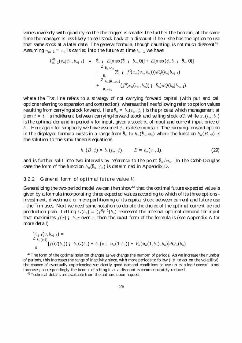
varies inversely with quantity so the the trigger is smaller the further the horizon; at the sametime the manager is less likely to sell stock back at a discount if he / she has the option to usethat same stock at a later date. The general formula, though daunting, is not much di®erent42.Assuming un¡1 = vn is carried into the future at time tn¡1 we have:

V 0n¡1(vnjφn, bn¡1) = ebn ¡ E[max(ebn ¡ bn, 0)] + E[max(φnbn ¡ ebn, 0)]

¡Z ebn/φn

ebn

(ebn ¡ f 0(xn(vn, bn)))dQ(bnjbn¡1)

+Z hn(ebn,φn)

ebn/φn

(f 0(xn(vn, bn)) ¡ ebn)dQ(bnjbn¡1),

where the ¯rst line refers to a strategy of not carrying forward capital (with put and calloptions referring to expansion and contraction), whereas the lines following refer to option valuesresulting from carrying stock forward. Here ebn = bn(vn, φn) is the price at which management attiem t = tn is indi®erent between carrying-forward stock and selling stock o®, while xn(vn, bn)is the optimal demand in period n for input, given a stock vn of input and current input price ofbn. Here again for simplicity we have assumed φn is deterministic. The carrying-forward optionin the displayed formula exists in a range from ebn to hn(ebn, φn) where the function hn(B,φ) isthe solution to the simultaneous equations

hn(B, φ) = bn(vn, φ), B = bn(vn, 1), (29)

and is further split into two intervals by reference to the point ebn/φn. In the Cobb-Douglascase the form of the function hn(ebn, φn) is determined in Appendix D.

3.2.2 General form of optimal future value Vn

Generalizing the two-period model we can then show43 that the optimal future expected value isgiven by a formula incorporating three expected values according to which of its three options -investment, divestment or mere partitioning of its capital stock between current and future use- the ¯rm uses. Next we need some notation to denote the choice of the optimal current-periodproduction plan. Letting G(bn) = (f 0)¡1(bn) represent the internal optimal demand for inputthat maximizes f(x) ¡ bnx over x, then the exact form of the formula is (see Appendix A formore detail)

Vn¡1(v, bn¡1) =Z bn(v,1)

0[f(G(bn)) ¡ bnG(bn) + bn(v ¡ bun(1, bn)) + Vn(bun(1, bn), bn)]dQn(bn)

42The form of the optimal solution changes as we change the number of periods. As we increase the numberof periods, this increases the range of inactivity since, with more periods to follow (i.e. to act on the volatility),the chance of eventually experiencing su±ciently good demand conditions to use up existing \excess" stockincreases; correspondingly the bene¯t of selling it at a discount is commensurately reduced.

43Technical details are available from the authors upon request.

26

+Z bn(v,φn)

bn(v,1)[f(v ¡ un(v, bn)) + Vn(un(v, bn), bn)]dQn(bn)

+Z 1

bn(v,φn)[f(G(φnbn)) ¡ φnbnG(φnbn) + φnbn(v ¡ bun(φn, bn)) + Vn(bun(φn, bn), bn)]dQn(bn).

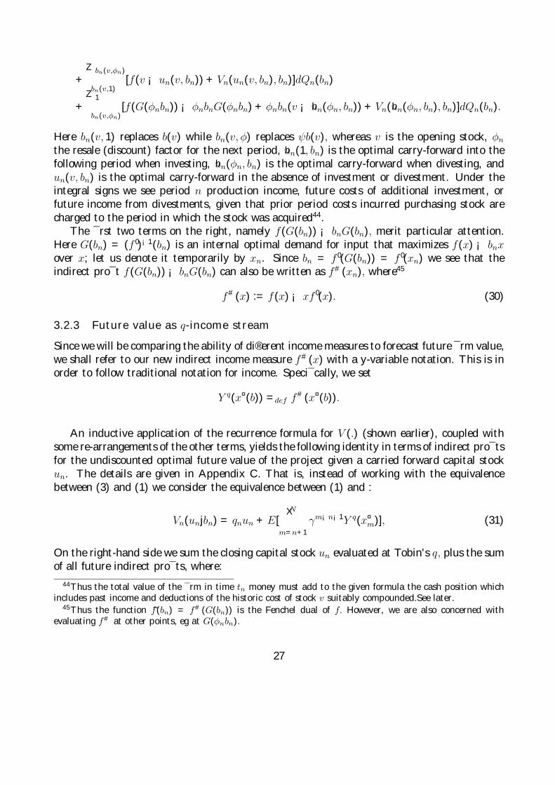
Here bn(v, 1) replaces b(v) while bn(v, φ) replaces ψb(v), whereas v is the opening stock, φn

the resale (discount) factor for the next period, bun(1, bn) is the optimal carry-forward into thefollowing period when investing, bun(φn, bn) is the optimal carry-forward when divesting, andun(v, bn) is the optimal carry-forward in the absence of investment or divestment. Under theintegral signs we see period n production income, future costs of additional investment, orfuture income from divestments, given that prior period costs incurred purchasing stock arecharged to the period in which the stock was acquired44.

The ¯rst two terms on the right, namely f(G(bn)) ¡ bnG(bn), merit particular attention.Here G(bn) = (f 0)¡1(bn) is an internal optimal demand for input that maximizes f(x) ¡ bnxover x; let us denote it temporarily by xn. Since bn = f 0(G(bn)) = f 0(xn) we see that theindirect pro¯t f(G(bn)) ¡ bnG(bn) can also be written as f#(xn), where45

f#(x) := f(x) ¡ xf 0(x). (30)

3.2.3 Future value as q-income stream

Since we will be comparing the ability of di®erent income measures to forecast future ¯rm value,we shall refer to our new indirect income measure f#(x) with a y-variable notation. This is inorder to follow traditional notation for income. Speci¯cally, we set

Y q(x¤(b)) =def f#(x¤(b)).

An inductive application of the recurrence formula for V (.) (shown earlier), coupled withsome re-arrangements of the other terms, yields the following identity in terms of indirect pro¯tsfor the undiscounted optimal future value of the project given a carried forward capital stockun. The details are given in Appendix C. That is, instead of working with the equivalencebetween (3) and (1) we consider the equivalence between (1) and :

Vn(unjbn) = qnun + E[NX

m=n+1γm¡n¡1Y q(x¤m)], (31)

On the right-hand side we sum the closing capital stock un evaluated at Tobin's q, plus the sumof all future indirect pro¯ts, where:

44Thus the total value of the ¯rm in time tn money must add to the given formula the cash position whichincludes past income and deductions of the historic cost of stock v suitably compounded.See later.

45Thus the function ~f(bn) = f#(G(bn)) is the Fenchel dual of f. However, we are also concerned withevaluating f# at other points, eg at G(φnbn).

27

i)Y (x) = f#(x) = f(x) ¡ xf 0(x) denotes the indirect pro¯t function associated with the pro-duction function f(x);ii) um+1 = um+1(umjbn, ..., bm) is the optimal carry-forward from period m to period m+1 giventhe price history bn, ..., bm;iii) x¤m = x¤m(um¡1, bm) is the general optimal demand for input at time m (so that when the¯rm expands x¤m = G(bm));iv) qm = qm(um, bm) is the period-m Tobin's marginal q, de¯ned as the average marginal bene¯tof utilization of a unit of input in period m (given the current value of bm and the closingstock um of the current period). When um is selected optimally (given opening stock vm) thediscounted value of qm ranges between replacement cost bm and resale cost φmbm. Indeed whenum takes the value corresponding to optimal expansion, discounted qm is the replacement costand similarly when um takes the value corresponding to optimal contraction, discounted qm

takes the value φmbm.Rewriting the identity thus

γ[Vn(unjbn) ¡ qnun] = E[NX

m=n+1γm¡nY (x¤m)] = V #

n (unjbn), (32)

we see that the lefthand-side is the discounted future value less its marginal cost, and we denotethis quantity by γV #

n (unjbn), consistently so, since qn = V 0n.

Our analysis of assessing future value shows the importance of Tobin's q, i.e. of marginalbene¯t, and we stress that this refers to replacement cost, as such, only in the expansion regime.It is natural therefore to measure current earnings as well by reference to Tobin's q, especiallyas both current demand and future demand have equal marginal value at an optimum (aftertaking due note of appropriate discounting).

De¯nition: The q-income at time tn is the indirect pro¯t, namely, the revenue lessmarginal cost of input, in symbols f(xn) ¡ xnf 0(xn), i.e. f#(xn), where xn and un have beenchosen to optimise the expression

f(xn) + cn(xn + un ¡ vn) + γVn(un, bn),

given vn, and where cn = bn for xn + un ¡ vn > 0 and cn = φnbn for xn + un ¡ vn < 0.

We note that q as introduced above is characterized along the lines of ADEP as beingcomposed of:- a certainty-equivalent price less the put option to expand plus the call option to contract plusthe option to carry forward unused stock, i.e. typically it is of the form

q0 = eb1 ¡ E[max(eb1 ¡ b1, 0)] + E[max(φ1b1 ¡ eb1, 0)]

+Z h(eb1,φ)eb1

(f 0(x1(u, b1)) ¡ eb1)dQ(b1jb0) (33)

28

for some function h and so includes the option to expand, to contract and to carry-forwardoptimally. Note that the future value of the ¯rm, as measured in time tn+1 values, associatedwith the end of the production period [tn, tn+1], is

Y (x¤n) + γVn = Y (x¤n) + γqnun + E[NX

m=n+1γm¡nY (x¤m)].

So recalling (1) and (3), we now see that we may write down the ¯rm equity value Sn in termsof its book-value Bn at time tn (i.e. the cash position kn plus historic cost hnvn of openingstock vn), by means of the following identity:

Sn = Bn + Y (x¤n) + vn ¢ HGn + E[NX

m=n+1γm¡nY (x¤m)], (34)

where HGn denotes the holding gain (per unit) on opening stock, and takes the followingvalue, given a historic valuation of hn per unit:(U) HGn = bn ¡ hn, (IO) HGn = γqnbn ¡ hn, (RO) HGn = φnbn ¡ hn.

Alternatively the equity value may be expressed in terms of the cash position kn at time tnand the corresponding opening stock position vn as

Sn = kn + γqn ¢ vn + Y (x¤n) + E[NX

m=n+1γm¡nY (x¤m)]. (35)

In words: the equity value comprises opening cash, q-revalued opening stock, current q-incomeand future q-income V #. We recall that the q-revaluation price of stock is either bn (i.e.replacement cost) in regime (U), or φnbn (i.e. resale price) in regime (RO) or an intermediatevalue in regime (IO).

To summarize, our approach considers an alternative valuation identity and generalizes theearlier two-period model to multiple periods. After taking appropriate discounting, the formof the optimal value function V (.) comprises:

-q adjusted value of the closing capital stock- plus the expected q-income stream.

Moreover we have established the form of Y (x¤n(bn)) given a Cobb-Douglas technology (seeAppendix B for the general details). It is satisfying that the q-income in this case is proportionalto the revenue. For the square root function speci¯cally:- the period n indirect pro¯t function Y (x¤n(bn)) takes a notionally simple form; it is 1/bn whenthe project is under-invested, 1/(φnbn) when it is over-invested, and an intermediate value inthe third regime.

29

Thus for our simple square-root returns model we can identify Vn(unjbn) by forming expec-tations over the input price process bn. Furthermore forming this expectation simply requireslooking at the appropriately censored integral of the next input price and the censoring valueis the current input price bn times a factor gn, a generalized version46 of (24).

Remark 9: (Existence of an Informational Asymmetry) We have shown how amanager determines the optimal expected future value of the ¯rm by appropriatevaluation of embedded put and call options. We must now ask why couldn't anexternal investor also directly identify the optimal value without the need to referto other (subsidiary) information such as accounting income data.

3.2.4 Informational asymmetry

We shall henceforth assume that whereas the internal manager observes bt, the investor doesnot. Thus at issue is whether some other accounting data may be helpful for the investor tryingto form inferences on the value of Vt(). Before embarking on this route we note that it could beargued that an investor reading the annual ¯nancial accounts could be able to infer the inputprice of capital from the movements in capital items in the accounts. Our response here is asfollows. Recall that in our introduction to the model we simpli¯ed the presentation by assumingthe returns function faced by the ¯rm was a simple square-root function and hence f#(xn) = 1

b ,that is once the q-theoretic operating pro¯t was reported an investor knows exactly the valueof b and then can readily determine the value for V (). Note though that our initial workingassumption of the square root function was simply to ease initial presentation. The importantresult we derive above (34) assumes only concavity of the returns function and in that caseobserving reported pro¯t (i) does not allow the investor to infer what b was directly, and (ii)even if the investor had some other means of ¯nding out the true value of b, that would stillnot be enough to infer the functional form of V () since in the case of the general Cobb-Douglasreturns function xθ (for which f#(x) = (1 ¡ θ)f(x)), the function V () cannot be recoveredfrom knowledge of b without knowledge of the technology returns parameter θ.That is, if thereader feels uneasy about our modelling assumption that b is unobservable to an investor, thenassuming that the general returns / technology factor θ is unobservable to the investor inducesthe same desired result that an investor cannot from an observed pro¯t ¯gure disentangle whatthe values for b and θ are - hence directly determine the optimal value function.

Fortunately since f#(x) is directly proportional to revenue f(x), the current marginal valuef 0(x) is proportional to the ratio of current revenue over current consumption x.So despite therelevant q-theoretic variable being the current marginal pro¯tability f 0(xn)/bn, it is appropriatefor an external investor to take an interest in f#(xn).

This identi¯cation of an asymmetry clearly raises the issue of optimal contract design withina principal-agent context47. We note that given our dynamic model setting, issues of dynamic

46We will give a speci¯c example in the next section below.47Our underlying model framework di®ers from that of Dutta and Reichelstein (1999) and Govindarajan

30

commitment and renegotiation will immediately arise and we leave to a following study thepursuit of these extensions. Our task here is to identify the ¯rst best. In contrast to mostsingle period agency models where this is a trivial issue, in our setting it is not, evidencedperhaps by the fact that Feltham and Ohlson have been working with a model over the lastdecade which clearly has not been ¯rst best (since it ignores option values).

Having identi¯ed how managers can determine the optimal future value of the ¯rm, and onthe assumption that an informational asymmetry exists between the manager and the investor,we now consider how the investor could use accounting measures to make inferences concerningthe future value of the ¯rm.

and Ramikrishnan (2001) because they assume that the change in cash °ow or earnings is linearly a®ected byexercise of e®ort on the part of the manager and do not recognise the option component of investment. As wehave seen this options component does not necessarily add to cash °ow or earnings in a linear way.

31

4 Using an Earnings Measure to Infer Firm Value

Given Remark 9 let us now consider how a representative investor could use an earnings measureto value a ¯rm. Recalling the fundamental FO result (4):

eyt+1 = ωeyt + xt + εt+1,

which has been used repeatedly by empiricists to test for the value relevance of accountingmeasures, at this stage we summarize our critique of this previous research via two remarks:

Remark 10: (Non-optimality of the FO Model)Since the FO model does not recognize real options that arise in practice it is hard to knowwhat (if anything) empirical tests48 using the FO speci¯cation actually mean for the decisionvalue signi¯cance of accounting measures. For instance, recalling our results on the underlyingnaivety of the investment model in the FO approach, we comment in subsection 4.3 that only inthe restrictive case of non stochasticity in the underlying parameter is the FO residual incomemodel consistent with our optimization model.

Remark 11: (Non-Linearity of the Firm Value)By explicitly recognizing the real options omnipresent with investment in real assets, we haveshown that the type of linear functional relationship embodied by (4), and used so frequentlyby empiricists49, is inappropriate except in special cases. Instead our real-options analysis,which brings to the fore the three distinct regimes of optimal investment behavior (contraction,maintenance and expansion), suggests that, rather than testing for accounting value relevancewith a single linear regression model, an approach using ¯nite-mixture (distribution) modelswith three regime changes may be appropriate. We stress that the implied linearities arebetween our chosen earnings measure and future value50.

At least two questions naturally arise from these remarks. What is the signi¯cance forearnings based valuation of the non optimality of FO residual income? If a simple linearregression is not representative of the underlying optimal investment environment what is anappropriate (perhaps approximate) empirical speci¯cation? We will address these questions inthe following two subsections respectively.

48Both Feltham and Ohlson have on occasion raised concerns about the empirical appllications of their model.Our critique here is with the claimed theoretical validity of empirical research claiming to apply the FO results.

49We shall discuss the extensions proposed by Burgsthaller and Dichev (1997) and others in subsection 4.2.50Alternatively we could look at the relationship between our measure of current earnings and market value

St by recovering the relationship from (34).

32

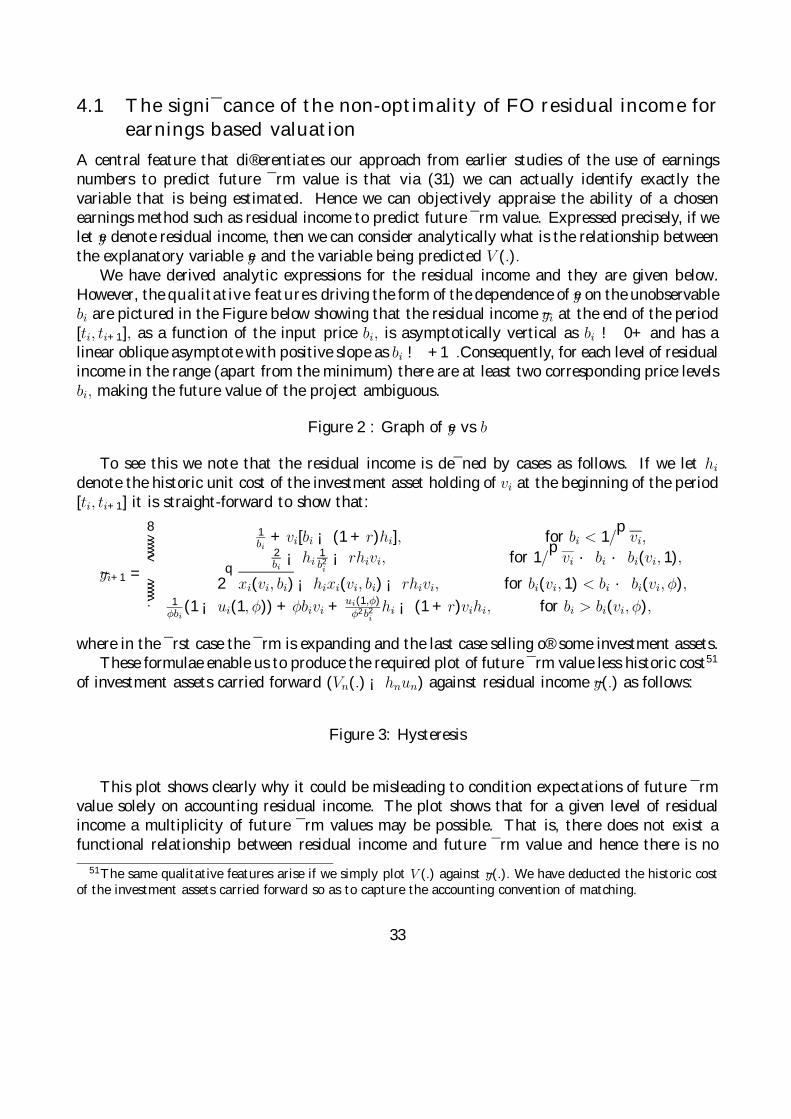
4.1 The signi¯cance of the non-optimality of FO residual income forearnings based valuation

A central feature that di®erentiates our approach from earlier studies of the use of earningsnumbers to predict future ¯rm value is that via (31) we can actually identify exactly thevariable that is being estimated. Hence we can objectively appraise the ability of a chosenearnings method such as residual income to predict future ¯rm value. Expressed precisely, if welet ey denote residual income, then we can consider analytically what is the relationship betweenthe explanatory variable ey and the variable being predicted V (.).

We have derived analytic expressions for the residual income and they are given below.However, the qualitative features driving the form of the dependence of ey on the unobservablebi are pictured in the Figure below showing that the residual income ~yi at the end of the period[ti, ti+1], as a function of the input price bi, is asymptotically vertical as bi ! 0+ and has alinear oblique asymptote with positive slope as bi ! +1.Consequently, for each level of residualincome in the range (apart from the minimum) there are at least two corresponding price levelsbi, making the future value of the project ambiguous.

Figure 2 : Graph of ey vs b

To see this we note that the residual income is de¯ned by cases as follows. If we let hi

denote the historic unit cost of the investment asset holding of vi at the beginning of the period[ti, ti+1] it is straight-forward to show that:

~yi+1 =

8>>>>><>>>>>:

1bi+ vi[bi ¡ (1 + r)hi], for bi < 1/

pvi,

2bi

¡ hi1b2i

¡ rhivi, for 1/p

vi · bi · bi(vi, 1),

2q

xi(vi, bi) ¡ hixi(vi, bi) ¡ rhivi, for bi(vi, 1) < bi · bi(vi, φ),1

φbi(1 ¡ ui(1, φ)) + φbivi + ui(1,φ)

φ2b2ihi ¡ (1 + r)vihi, for bi > bi(vi, φ),

where in the ¯rst case the ¯rm is expanding and the last case selling o® some investment assets.These formulae enable us to produce the required plot of future ¯rm value less historic cost51

of investment assets carried forward (Vn(.) ¡ hnun) against residual income ~y(.) as follows:

Figure 3: Hysteresis

This plot shows clearly why it could be misleading to condition expectations of future ¯rmvalue solely on accounting residual income. The plot shows that for a given level of residualincome a multiplicity of future ¯rm values may be possible. That is, there does not exist afunctional relationship between residual income and future ¯rm value and hence there is no

51The same qualitative features arise if we simply plot V (.) against ~y(.). We have deducted the historic costof the investment assets carried forward so as to capture the accounting convention of matching.

33

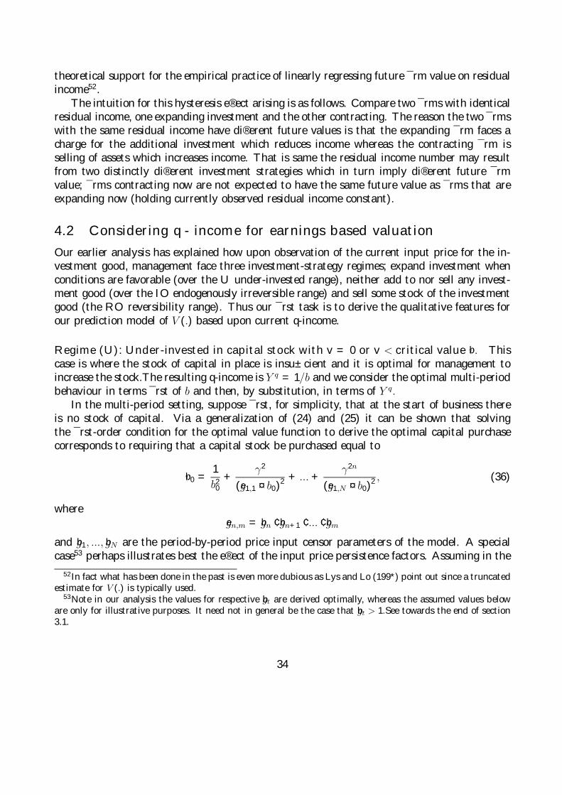
theoretical support for the empirical practice of linearly regressing future ¯rm value on residualincome52.

The intuition for this hysteresis e®ect arising is as follows. Compare two ¯rms with identicalresidual income, one expanding investment and the other contracting. The reason the two ¯rmswith the same residual income have di®erent future values is that the expanding ¯rm faces acharge for the additional investment which reduces income whereas the contracting ¯rm isselling of assets which increases income. That is same the residual income number may resultfrom two distinctly di®erent investment strategies which in turn imply di®erent future ¯rmvalue; ¯rms contracting now are not expected to have the same future value as ¯rms that areexpanding now (holding currently observed residual income constant).

4.2 Considering q - income for earnings based valuationOur earlier analysis has explained how upon observation of the current input price for the in-vestment good, management face three investment-strategy regimes; expand investment whenconditions are favorable (over the U under-invested range), neither add to nor sell any invest-ment good (over the IO endogenously irreversible range) and sell some stock of the investmentgood (the RO reversibility range). Thus our ¯rst task is to derive the qualitative features forour prediction model of V (.) based upon current q-income.

Regime (U): Under-invested in capital stock with v = 0 or v < critical value bv. Thiscase is where the stock of capital in place is insu±cient and it is optimal for management toincrease the stock.The resulting q-income is Y q = 1/b and we consider the optimal multi-periodbehaviour in terms ¯rst of b and then, by substitution, in terms of Y q.

In the multi-period setting, suppose ¯rst, for simplicity, that at the start of business thereis no stock of capital. Via a generalization of (24) and (25) it can be shown that solvingthe ¯rst-order condition for the optimal value function to derive the optimal capital purchasecorresponds to requiring that a capital stock be purchased equal to

bv0 =1b20

+γ2

(eg1,1 ¤ b0)2 + ... +

γ2n

(eg1,N ¤ b0)2 , (36)

whereegn,m = bgn ¢ bgn+1 ¢ ... ¢ bgm

and bg1, ..., bgN are the period-by-period price input censor parameters of the model. A specialcase53 perhaps illustrates best the e®ect of the input price persistence factors. Assuming in the

52In fact what has been done in the past is even more dubious as Lys and Lo (199*) point out since a truncatedestimate for V (.) is typically used.

53Note in our analysis the values for respective bgt are derived optimally, whereas the assumed values beloware only for illustrative purposes. It need not in general be the case that bgt > 1.See towards the end of section3.1.

34

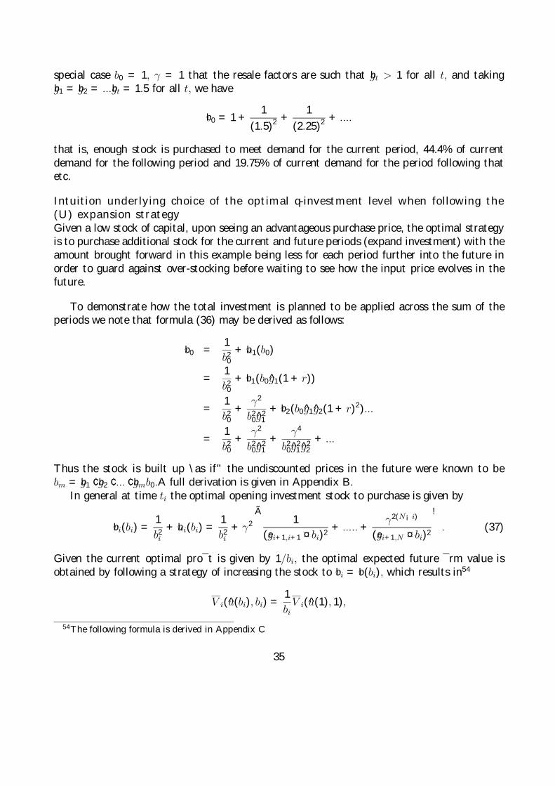
special case b0 = 1, γ = 1 that the resale factors are such that bgt > 1 for all t, and takingbg1 = bg2 = ...bgt = 1.5 for all t, we have

bv0 = 1 +1

(1.5)2+

1(2.25)2

+ ....

that is, enough stock is purchased to meet demand for the current period, 44.4% of currentdemand for the following period and 19.75% of current demand for the period following thatetc.

Intuition underlying choice of the optimal q-investment level when following the(U) expansion strategyGiven a low stock of capital, upon seeing an advantageous purchase price, the optimal strategyis to purchase additional stock for the current and future periods (expand investment) with theamount brought forward in this example being less for each period further into the future inorder to guard against over-stocking before waiting to see how the input price evolves in thefuture.

To demonstrate how the total investment is planned to be applied across the sum of theperiods we note that formula (36) may be derived as follows:

bv0 =1b20

+ bu1(b0)

=1b20

+ bv1(b0g1(1 + r))

=1b20

+γ2

b20g21+ bv2(b0g1g2(1 + r)2)...

=1b20

+γ2

b20g21+

γ4

b20g21 g22+ ...

Thus the stock is built up \as if" the undiscounted prices in the future were known to bebm = bg1 ¢ bg2 ¢ ... ¢ bgmb0.A full derivation is given in Appendix B.

In general at time ti the optimal opening investment stock to purchase is given by

bvi(bi) =1b2i

+ bui(bi) =1b2i

+ γ2

Ã1

(egi+1,i+1 ¤ bi)2+ ..... +

γ2(N¡i)

(egi+1,N ¤ bi)2

!. (37)

Given the current optimal pro¯t is given by 1/bi, the optimal expected future ¯rm value isobtained by following a strategy of increasing the stock to bvi = bv(bi), which results in54

V i(u(bi), bi) =1bi

V i(u(1), 1),

54The following formula is derived in Appendix C

35

where the bar denotes expectation over the future resale factor φi+1. This homogeneity is derivedin Appendix E. Notationally we may write this optimal expected value in the form

bVi =Ci;N

bi, (38)

for some constant Ci;N = V i(bu(1), 1). That is, qualitatively - the optimal future value of the¯rm is given by the q-pro¯t Y q

i = 1/bi multiplied by a certain constant55 (which is dependenton volatility):

bVi = Y qi ¢ Ci;N . (39)

Regime (RO): Over-stocked in capital stock with some excess sold o® The case ofa costly divestment is quite similar. For a given price bn there are now two benchmark stocklevels. The ¯rst and lower value is the optimum level bvn (computed as above) below which thestock level should not fall but there is now a second, larger, upper optimum level bvn(φn, bn),dependent also on the current resale rate, above which the stock should not rise. The ¯rstorder condition (20) implies that current demand is as though the resale price was the purchaseprice so that the q-income is now Y q

n = 1/(φnbn). Again one considers optimal multi-periodbehaviour ¯rst in terms of bn and then, by substitution, in terms of Yq,n.

At time tn the optimal highest stock level worth keeping exists and is given by

bvn(φn, bn) =1

(bnφn)2+

γ2

(bnφngn(φn))2

"1 +

γ2

eg2n+2,n+2+ ... +

γ2(N¡n)

eg2n+2,N

#,

i.e. as though the current price were φnbn and discounted future prices were to be γbn+1 = φnbn ¢gn(φn), γ2bn+2 = φnbngn(φn)bgn+2, ..., γmbn+m = φnbn ¢ gn(φn)egn+2,n+m, ... . Corresponding tobvn(φn, bn) there is an optimal current revenue from production, namely 1/(φnbn), and an optimalcarry-forward bun(φn, bn) = bvn(φn, bn) ¡ 1/(bnφn)2, i.e. of the form bun(φn, bn) = bun(φn, 1)/b2n.Note that in our notation bun(φn, 1) = bun(φn)/φ2

n to ensure that bvn(φn, bn) = (1+bun(φn))/(φ2nb2n).

Intuition underlying choice of the optimal investment level when following the (RO)expansion strategyGiven a large stock of capital, upon seeing an advantageous resale rate, the optimal strategyis to sell some of the additional (investment) stock that was planned for use in this and futureperiods (contract investment), but the amount sold forward is less for each period further intothe future that we consider; this is because the longer we wait the more chance there is thatthe ¯rm could move into an under-stocked position. Hence, analogously to the (U) regime, thefuture value from carrying-forward is:

Vn(bun(φn, bn), bn) =1bn

Vn(bun(φn, 1), 1),

55We note that this last equation also holds in the general Cobb-Douglas case (for an appropriate rede¯nedconstant).

36

(where the bar recalls the expectation over the future resale rate). We can again rewrite the

displayed formula as: bV φn =

Cφn,N

φnbn,where Cφ

n,N = φnVn(bun(φn, 1), 1). This, as before, follows fromthe general formula of Appendix E. Again we have a linear relationship:

bV φn = Y q

n ¢ Cφn,N , (40)

between future value56 and accounting pro¯t Y qn = 1/(φnbn).

Regime (IO): Given φn < 1 and the ¯rm is neither over-invested nor under-investedHere we are concerned with the intermediate input price range:

bn = bn(v, 1) < bn < bn(v, φn) = bn. (41)

The revenue is, as always,2q

xn(vn, bn),

so we set the q-pro¯t to beY q

n = Y q(x¤n) =q

xn(vn, bn),

as required by our formula since f#(x) =p

x. Thus we have, since xn(vn, bn) = 1/bn2 and

xn(vn, bn) = 1/bn2, that

Y qn (bn) =

1bn

, Y qn (bn) =

1φnbn

,

so the intermediate input price range corresponds to

1bn

< Y qn <

1φnbn

,

as 1/bn > 1/bn and 1/bn < 1/bn. In this range the ¯rm neither invests nor divests. It parti-tions its stock vn into current optimal consumption xn(vn, bn) and investment carried forwardun(vn, bn), and the cash income in this range is thus

2q

xn(vn, bn).

The relation between the expected future ¯rm value and q-income is then given57 by:

Vn = Vn(vn ¡ (Y qn )

2, bn(Y qn )),

where bn = bn(Y qn ) solves

Y qn =

qxn(vn, bn).

Remark 12: (Monotonicity of V #n in Y q

n )56Again this last equation holds good in the general Cobb-Douglas case (for an appropriate constant).57Observe that dVn

dYn= ∂Vn

∂u (¡2Yn) + ∂Vn∂b (dYn

dbn)¡1 < 0 if ∂Vn

∂b > 0.

37

Provided either the volatility is large enough, i.e. σ ¸ σ¤(φn+1), or, equivalently, provided theforthcoming discount factor φn+1 is close enough to unity, i.e. φ¤n+1(σ) · φn+1 < 1,the functionV # regarded as a function of Y q

n is monotonic increasing. For instance, in a two-period model,a su±cient bound is provided by the inequality

φ1 > exp(¡1.65σ).

See Appendix H.

4.2.1 Convexity of future ¯rm value in q-income

To compare our model predictions with thosed derived in the literature, we need to considerthe equity value of the ¯rm given its current q-income Y q.A plot follows.

Figure 4: Graph of S vs Y q

The graph has three sections correponding to the three regimes considered earlier. Wecomment on the qualitative features. For small enough value of Y q (i.e. less than Y q) theequity value of the ¯rm takes a convex (in fact hyperbolic) form58

vn

Y q ¡ vnh + o(Yq)

in the square-root case (the ¯rst term generalizing to vnY ¡α/(1¡α), in the case of a Cobb-Douglasindex α). For large values of Y q (i.e. greater than Y q) the equity value is asymptotically linearand takes the form

(2 + V (u(1), 1))Y q ¡ vnh + vn(Y q)¡α/(1¡α).

One may take the view that on our de¯nition of income Y q this quantity is unlikely to be verysmall and so the vertical asymptote is in itself is irrelevant, but the \convexity" it exhibits isnot out of line with the cluster-plot given in Burgstahler and Dichev (B&D).

To see how this relates to the Burgstahler and Dichev (1997) ¯ndings, recall that in essencethe B&D paper empirically tests the future value of a ¯rm by a two-period model. In the laterof the two periods the earnings E1 predict a possible future earnings stream valued at W 1

1 = cE1

(where c is the earnings capitalization factor). Management have the option to switch fromthis earnings stream to an alternative activity. That activity also generates a future earningsstream W 2

1 , known as adaptation value, which is a constant independent of E1 and assumed¯xed a priori at a value A. The model's empirical proxy for A is the book value B0. The ¯rmcurrently has earnings E0, so the current market value of the ¯rm S0 comprises book value B0,the current earnings E0, and the expected value V0 of the claim: maxfW 2

1 , W 21 g = maxfcE1, Ag.

In a log-normal setting for the distribution of E1 given E0, the value V0 has the well-knownconvex shape of a call-value struck at K = A/c. Our model agrees with the linear valuationW 1

1 = cE1 but only provided E1 is large enough. On the other hand, our model does not give58In fact, the exact form is φnbn(vn ¡ u(φ, 1)/b2) + 1

bnV (u(φ, 1), 1) + 1

φbn¡ hnvn

38

management the option to receive a ¯xed income stream A for values of E1 below some strikevalue K. Instead the adaptation value depends on the value of E1 and is at best viewed aspiecewise linear in E1 with ranges of linearity endogenously de¯ned by Y q and Y q as given by(??). Note that B&D also subdivide the earnings range into three intervals in order to verifyconvexity (by testing whether the slope of the respective best linear ¯t to the data is increasing).Another interestin point is that presumably in order to ensure large enough subsample sizes,B&D chose to have equal numbers of observations in each interval. Given the option-valuationbasis for their model, it would have been economically more intuitive had they selected theirmiddle interval centered on the implied option strike K.

To summarize our ¯ndings are in broad agreement with the stylized facts proposed by B&Din their option style valuation model. That is our model predicts asymptotic linearity for largevalues of current earnings and a convex valuation for low current earnings. However, in ourmodel the market value can be negatively relatated to (low) earnings as was observed by B&Din their empirical study. Whereas they could provide no formal explanation our model showsit may be consistent ¯rm optimization with non constant abandonment value.

Before moving to the concluding section we shall now present a subsection which shows thatresidual income is in fact a special case (under restrictive conditions) of q-income and hencein these special circumstances applying FO residual income is consistent with optimality ofinvestment behaviour.

4.3 The Equivalence Between Residual Income and q-Theoretic Op-erating Pro¯t: Intuition Underlying the Special Case

We start by recalling the example of subsection 2.1. Working with current value residual incomewe have from (9) that

eyCV1 = 2

px ¡ b0x, eyCV

2 = 2p

u ¡ b1u.

Noting that by suitable rede¯nition of notation and introducing a time script, if

b0(1 + r) = b1

theneyCV1 = 2

px0 ¡ bx0 = Y (x¤0), eyCV

2 = 2p

x1 ¡ bx1 = Y (x¤1).

That is, provided x0 = x¤0 = ( 1b0)2 and x1 = x¤1 = ( 1

b1)2, the current value residual income is

identical to q-theoretic operating pro¯t. This simple example shows how management focusingupon residual income is a special case of adopting a focus upon q-theoretic operating pro¯t.Speci¯cally the equivalence holds in the restricted case that the discounted input prices areconstant through time. This result is just another recurrence of what we have establishedearlier: focusing upon residual income does not take into account the put and call, expansionand contraction options that arise with investment decisions taken in a stochastic environment.Only in the special case where those options have no value, because the input price is constant

39

(non stochastic), will prediction relative to the two respective measures be equivalent. To seethis recall (35) -

Sn = kn + γqn ¢ vn + Y (x¤n) + E[NX

m=n+1γm¡nY (x¤m)],

- and that optimization is with respect to current production xn and future stock carried forwardun. What is appealing about (35) is that, since qn includes the value59 of embedded put and calloptions and of carrying forward stock, the optimization problem is essentially separable - thatis, after identi¯cation of Tobin's qn, management can think about current period optimizationover x independently of expansion or contraction decisions for the overall level of investmentstock to carry forward un. With reference to equation (34)

Sn = Bn + Y (x¤n) + vn ¢ HGn + E[NX

m=n+1γm¡nY (x¤m)],

note that in the case when the input price b is ¯xed, the γqnun term cancels against the marketprice paid for the stock (zero holding gains), and

Yn(x¤n(bn)) = eyCVn (x¤n(bn)).

However, note the converse, when γqnun 6= bn, then Yn(x¤n(bn)) 6= eyCVn (exn(bn)).

5 ConclusionFor the FO model recall that FO superimpose (4) and (5) on (3). However, as has been arguedextensively above, superimposing this simple AR(1) process on the way residual income grows,considerably restricts the type of underlying investment behavior that could be consistent withthe model. The objective of the paper has been to establish a more °exible model whichfacilitates an alternative representation of the expected income stream of terms Et(eyt+τ) basedupon optimal managerial real-options evaluation. These ¯ndings are signi¯cant because theFeltham-Ohlson valuation framework has been used by empiricists to test the value relevanceof accounting data. Some researchers have criticized how empiricists have used the model totry to specify appropriate empirical testing procedures for the value relevance of accountinginformation. We address both the underlying validity of the FO model and the implications forspeci¯cation of empirical testing routines. With regard to validity, we show how, independentlyof speci¯cations issues, the underlying constant growth assumption which is central to theFeltham-Ohlson framework removes the possibility for management to have a role in decidingwhether or not to exercise expansion and contraction possibilities which do occur with mostinvestment projects. Given this limitation we develop an alternative valuation framework whichdoes not su®er from these limitations because the option to expand or contract optimally isgiven centre-stage in our model of managerial decision-making. This °exible model which puts

59Recall (33).

40

three investment regimes at center stage also shows that a single linear regression model of thelink between ¯rm value and accounting measures is inappropriate. Instead our model showshow a regime-shifting speci¯cation (giving rise to a tri-mixture of distributions) would moree®ectively capture the underlying statistical relationships that apply. In the previous section wehave derived the basic regime functional forms needed to implement such testing procedures.

41

Abel, A.B., and Eberley, J.C., (1996), \Optimal Investment with Costly Reversibility", Reviewof Economic Studies.Abel, A.B., Dixit, A.K., Eberley, J.C. and Pindyck, R.S., (1996), \Options, the Value of Capital,and Investment", Quarterly Journal of Economics.Biddle,G.C., Chen,P., and Zhang, G., (2000), \When Capital Follows Pro¯tability: Non-linearResidual Income", working paper Hong Kong University of Science and Technology.Burgstahler, D.C., and Dichev, I.D., (1997), \Earnings, Adaptation and Equity Value", Ac-counting Review, Vol 72, No.2.Dixit, A.K., and Pindyck, R.S., (1994), \Decision Making Under Uncertainty", Princeton Uni-versity Press.Dutta, S., and Reichelstein, S., (1999), \Asset Valuation and Performance Measurement in aDynamic Agency Setting", Review of Accounting Studies, vol. 4.Feltham, G.A. and Ohlson, J.A., (1995), \Valuation and Clean Surplus Accounting for Oper-ating and Financial Activities", Contemporary Accounting Research, 11, 689-731.Gietzmann, M.B., Ostaszewski, A.J., (1999), \Hedging the Purchase of Direct Inputs in anIn°ationary Environment", Management Accounting Research, 10, 61-84.Govindaraj, S., and Ramakrishnan, R.T.S., (2001), \Accounting Earnings Processes, Inter-Temporal Incentives and Their Implications for Valuation", Review of Accounting Studies, 6,427-457.Hopp, W. and Nair, S., (1991), \Timing Equipment Replacement Decisions Due to Discontin-uous Technological Change", Naval Research Logistics, 38, 203 - 220.Lo, K. and Lys, T., (2000), \The Ohlson Model: Contribution to Valuation Theory, Limitationsand Empirical Applications", Journal of Accounting Auditing and Finance.Ohlson, J.A., (1995), \Earnings, Book Values, and Dividends in Equity Valuation", Contem-porary Accounting Research, 11, 661-687.Peasnell, K.V. (1982), \Some Formal Connections Between Economic values and Yields andAccounting Numbers", Journal of Business Finance and Accounting, 361-381.Trigeorgis L., (1996), \Real Options", MIT Press, Cambridge.Yee, K.K. (2000), \Opportunities Knocking: Residual Income Valuation of an Adaptive Firm",Journal of Accounting Auditing and Finance.Varian, H.R., (1992), \Microeconomic Analysis", 3rd Edition, W. W. Norton.Walker, M., (1997), \Clean Surplus Accounting Models and Market Based Accounting Research:A Review", Accounting and Business Research.Zhang, G., (2000), \Accounting Information, Capital Investment Decisions, and Equity Valua-tion: Theory and Empirical Implications", Journal of Accounting Research, Vol 38, No. 2, 271-295.

42

6 Appendix A: NPV RuleIn this section we derive the NPV Rule. The notation (see section 3.2) is as follows: Fn(v, b0, φ),or simply F (v, b0, φ) with time tn suppressed, denotes the discounted future maximum expectedpro¯t ignoring the historic cost of the carry{forward input v. The price at the time tn is heredenoted b0 (sic!) and so that the price at time tn+1 is then b1;the resale rate revealed at timetn+1 is φ. When the time tn is suppressed ¹F+(v, b1) denotes expectation over φ0 of Fn+1(v, b1, φ0).Thus, for example F0(v, b0, φ) = γV0(v, b0, φ) and the corresponding value of the ¯rm ignoringpast costs and revenues is V0(vjb0) = f(G(b0)) ¡ b0G(b0) + F1(v, b0, φ). Now we have

γ¡1F (v, b0, φ) =Z b(v,1)

0

hf#(G(b1)) + b1(v ¡ bu(1, b1)) + F+(bu(1, b1), b1)

idQ1

+Z b(v,φ)

b(v,1)

hf(v ¡ u(v, b1)) + F+(u(v, b1), b1)

idQ1

+Z 1

b(v,φ)

hφb1(v ¡ bu(φ, b1)) + f#(G(φb1)) + F+(bu(φ, b1), b1)

idQ1.

Hence proceeding formally and applying the Liebniz Rule60

γ¡1F 0(v, b0, φ) =Z b(v,1)

0b1dQ1

+Z b(v,φ)

b(v,1)

hf 0(v ¡ u(v, b1))(1 ¡ u0) + F+

0(u(v, b1), b1)u0idQ1

+Z 1

b(v,φ)φb1dQ1.

But f 0(v ¡ u(v, b1)) = F+0(u(v, b1), b1) by de¯nition of u(v, b1). So

F 0(v, b0, φ) =Z b(v,1)

0b1dQ1 +

Z b(v,φ)

b(v,1)f 0(v ¡ u(v, b1))dQ1 +

Z 1

b(v,φ)φb1dQ1.

Hence

γ¡1F 0(u, b0, φ) =Z b(u,1)

0b1dQ1 +

Z b(u,φ)

b(u,1)f 0(x(u, b1))dQ1 +

Z 1

b(u,φ)φb1dQ1,

=Z eb10

b1dQ1 +Z h1(eb1,φ)eb1

f 0(x(u, b1))dQ1 +Z 1

h1(eb1,φ)φb1dQ1,

= eb1 +Z eb10

(b1 ¡ eb1)dQ1 +Z h1(eb1,φ)eb1

(f 0(x(u, b1)) ¡ eb1)dQ1

+Z 1

h1(eb1,φ)(φb1 ¡ eb1)dQ1.

60We do not show cancelling terms.

43

7 Appendix B: The optimal replenishment policy.We prove the following Recurrence Lemma

un(bn, φn+1) = G(bn+1(bn)) + un+1(bn+1(bn), φn+2).

Proof. Recall that the function u = un(b, φ) is de¯ned by the equation61

F 0n(u, b) = φb.

We work inductively. To obtain the solution v = un(bn, φn+1) of the ¯rst-order condition

F 0n(v, bn) = φn+1bn

we begin by ¯rst solving the censor equation

qn(B, φn+1, , bn) = φbn.

We denote the solution62 by bn+1(bn, φ). Recall that

qm(B, φm+1, bm) =Z B

0bmdQ(bmjbm¡1)

+Z hm(B,φm+1)

Bf 0(xm(vm(B), bm))dQ(bmjbm¡1) + φm+1

Z 1

hm(B,φm+1)bmdQ(bmjbm¡1).

Here vm(b) = G(b) + um(b, φm+1), and G(b) = ff 0g¡1(b). Now for an appropriate functionBn+1(v) we have

F 0n(v, bn) = qn(Bn+1(v), φn+1, bn),

so we now need to solveBn+1(bv) = bn+1(bn, φ).

But recalling that in general F (v, b) = f(v ¡ u(v, b) + F+(u, b), we have

F 0n(vn(b), b) = f 0(vn(b) ¡ u(vn(b), b))(1 ¡ u0) + F 0

n+1(u, b)u0

= f 0(vn(b) ¡ u(vn(b), b)) = b.

Thus we have the identity

Bn+1(vn(B)) = F 0n(vn(B), Bn+1(vn(B))) = B.

61Recall the convention that F = γV.62In the Cobb-Douglas case

bn+1(bn) = φbnbgn(φ)

for some constant bgn(φ).

44

Hence for B = bn+1(bn, φ) we have identi¯ed that bv = vnB. In conclusion we have

un(bn, φ) = G(bn+1(bn, φ)) + un+1(bn+1(bn, φ), 1)= G(bn+1(bn, φ)) + G(bn+2(bn+1(bn, φ), 1)) + ...

Corollary. The analysis prescribes an aggregate demand of

Dφn(bn) = G(bn+1) + ... + G(bn+i) + ...,

where G(b) = ff 0g¡1(b) and the sequence bn+i is given by the iteration

bn+1 = bn+1(bn, φ),bn+2 = bn+1(bn+1, 1),bn+3 = bn+3(bn+2, 1),

...

It is now easy to describe the replenishment programme. Suppose we have n periods remain-ing and we have a stock v. The acquisition programme calls for an optimal aggregate demandto be purchased of

D1n(bn) = G(bn+1) + ... + G(bn+i) + ...,

(i.e. with φ = 1) and either we have v below this amount in which case we need to top upto this amount or else we are moderately over-stocked and must carry-forward u¤n(v, φn+1, bn)without selling, or else we must sell to the point where the stock is Dφn+1

n (bn). Thus

u¤n(v, bn) =

8><>:

bun(1, bn) bn < bn(v, 1),u(v, bn) bn(v, 1) < bn < bn(v, φn+1),bun(φ, bn) bn(v, φn+1) < bn.

8 Appendix C: Derivation of Valuation formulaWe study ¯rst the general two-stage situation. The current price is b0 the next period price isb1 and the resale rate is φ. Our notation in this section for the maximum expected value givena stock v of inputs and given the knowledge of φ = φ1 is F (v, b0, φ); once b1 is revealed and uis carried forward into the future, the maximum expected revenue from the period beyond isF+(u, b1), where the bar signi¯es expectation over φ2.

We note that F = γV.

8.1 Step 1. We prove a recurrence

γ¡1F (v, b0, φ) = Eb1 [f#(x¤(v, b1)) + F+

#(u¤(v, b1), b1)] + γvq,

where the notation is as in section 3.2 above and is recalled below.

45

Proof. We have as in Appendix A that

γ¡1F (v, b0, φ) =Z b(v,1)

0

hf(G(b1)) ¡ b1G(b1) + b1(v ¡ bu(1, b1)) + F+(bu(1, b1), b1)

idQ1

+Z b(v,φ)

b(v,1)

hf(v ¡ u(v, b1)) + F+(u(v, b1), b1)

idQ1

+Z 1

b(v,φ)

hφb1(v ¡ bu(φ, b1)) + f#(G(φb1)) + F+(bu(φ, b1), b1)

idQ1.

To understand the ¯rst integral (corresponding to the understocked situation), note that theadditional purchase z is speci¯ed by v + z = G(b1) + bu(1, b1) and so the revenue is f(G(b1)) ¡b1(G(b1) + bu(1, b1) ¡ v).

Now we reorganize the expression on the right. First note that f#(x) = f(x)¡ xf 0(x), andsince G is the inverse of f 0 we have

f#(G(b1)) = f(G(b1)) ¡ b1G(b1).

Similarly F+¤(x) = F+(x) ¡ xF+

0(x). But since u = bu(1, b1) solves

b1 = γV 0+(u, b1) = F+

0(u, b1),

we haveF+

#(bu(1, b1), b1) = F+(bu(1, b1), b1) ¡ b1bu(1, b1).Likewise

F+#(bu(φ, b1), b1) = F+(bu(φ, b1), b1) ¡ φb1bu(φ, b1).

Lastly u = u(v, b1) solves

f 0(v ¡ u) = γV+0(u, b1) = F+

0(u, b1),

hence

F+#(u(v, b1), b1) = F+(u(v, b1), b1) ¡ u(v, b1)f 0(v ¡ u(v, b1))

= F+(u(v, b1), b1) ¡ u(v, b1)f 0(x(v, b1)),

where x(v, b1) = v ¡ u(v, b1). Of course

f#(x(v, b1)) = f(x(v, b1)) ¡ x(v, b1)f 0(x(v, b1))

We thus have, writing x for x(v, b1),

γ¡1F (v, b0, φ) =Z b(v,1)

0

hf#(G(b1)) + F+

#(bu(1, b1), b1)idQ1 + v

"Z b(v,1)

0b1dQ1

#

+Z b(v,φ)

b(v,1)

hf#(x) + F+

#(u(v, b1), b1)idQ1 +

Z b(v,φ)

b(v,1)[xf 0(x) + u(v, b1)f 0(x)] dQ1

+Z 1

b(v,φ)

hf#(G(φb1)) + F+

#(bu(φ, b1), b1)idQ1 + v

"Z 1

b(v,φ)φb1dQ1

#,

46

or just

γ¡1F (v, b0, φ) =Z b(v,1)

0

hf#(G(b1)) + F+

#(bu(1, b1), b1)idQ1

+Z b(v,φ)

b(v,1)

hf#(x) + F+

#(u(v, b1), b1)idQ1

+Z 1

b(v,φ)

hf#(G(φb1)) + F+

#(bu(φ, b1), b1)idQ1

+v"Z b(v,1)

0b1dQ1 +

Z b(v,φ)

b(v,1)f 0(x)dQ1 +

Z 1

b(v,φ)φb1dQ1

#.

This may be rendered in a more compact way as asserted above, namely

γ¡1F (v, b0, φ) = Eb1 [f#(x¤(v, b1)) + F+

#(u¤(v, b1), b1)] + vq,

provided we introduce the notation

x¤(v, b1) =

8><>:

G(b1) b1 < b(v, 1),x(v, b1) b(v, 1) < b1 < b(v, φ),G(φb1) b(v, φ) < b1,

and

u¤(v, b1) =

8><>:

bu(1, b1) b1 < b1(v, 1),u(v, b1) b1(v, 1) < b1 < b1(v, φ),bu(φ, b1) b1(v, φ) < b1,

wherex(v, b1) = v ¡ u(v, b1)

andq =

Z b1(v,1)

0b1dQ1 +

Z b1(v,φ)

b1(v,1)f 0(x(v, b1))dQ1 +

Z 1

b1(v,φ)φb1dQ1.

It is convenient to de¯ne a function h1 by the simultaneous equations

h1(B,φ) = b1(v, φ),B = b1(v, 1),

)

i.e. h1(B, φ) = b1(v1B, φ), where v = v1B solves B = b1(v, 1). We identify these functions in theCobb-Douglas case in a later section. In conclusion we may de¯ne an important function q0(B)as follows:

q0(B) =Z B

0b1dQ1 +

Z h1(B,φ)

Bf 0(x(vB, b1))dQ1 +

Z 1

h1(B,φ)φb1dQ1.

The solution for B of q0(B) = b0 is the censor eb1 = eb1(b0).

47

8.2 Step 2. Deduction from the Recurrence

We prove

V0(v, b0, φ) = E[NX

n=1γn¡1f#(x¤n(bn))] + vq0(b1(v, 1)),

or

F0(v, b0, φ) = E[NX

n=1γnf#(x¤n(bn))] + γvq0(b1(v, 1)).

Proof. We already know that

γ¡1F 0(v, b0) = V 0 = q(b(v, 1)) =Z b(v,1)

0bdQ(b) +

Z b(v,φ)

b(v,1)f 0(x(v, b))dQ(b) +

Z 1

b(v,φ)φbdQ(b)

(using generic notation), hence we may also write

V ¡ vq = γ¡1[F ¡ vqγ]= γ¡1[F (v, b0, φ) ¡ vF 0(v, b0)]= γ¡1F#(v, b0, φ)= Eb1 [f

#(x¤(v, b1)) + F+¤(u¤(v, b1), b1)].

Taking expectations over φ, we have

γ¡1F ¤(v, b0) = Eφ,b1 [f#(x¤(v, b1)) + F+

¤(u¤(v, b1), b1)].

We may now apply this result inductively, the ¯rst steps being

γ¡1F#0 (v, b0, φ) = Eb1 [f

#(x¤1(v, b1)) + F1#(u¤1(v, b1), b1)]

= Eb1 [f#(x¤1(v, b1)) + γEb2 [f

#(x¤2(u¤1, b2)) + F2

#(u¤2(u¤1, b2), b2)]]

= Eb1 [f#(x¤1(v, b1)) + γEb2 [f

#(x¤2(u¤1, b2)) + γEb3 [f

#(x¤3(u¤2, b3)) + F3

#(u¤3(u¤2, b3), b2)

= Eb1 [f#(x¤1(v, b1)) + Eb2 [γf#(x¤2(u

¤1, b2)) + Eb3 [γ

2f#(x¤3(u¤2, b3)) + γ2F3

#(u¤3(u¤2, b3),

Assuming N steps, so that FN+1 = 0, we obtain on suppressing some notation that

γ¡1F#0 (v, b0, φ1) = E[

NX

n=1γn¡1f#(x¤n(bn))].

So

V0(v, b0, φ1) ¡ vq1 = E[NX

n=1γn¡1f#(x¤n(bn))].

48

Rewriting, we obtain the valuation

f#(x¤0(v, b0)) + γV0(v, b0, φ1)

= f#(x¤0(v, b0)) + E[NX

n=1γnf#(x¤n(bn))] + vγq0(b1(v, 1)),

whereq0(B) =

Z B

0b1dQ1 +

Z h1(B,φ)

Bf 0(x(v1B, b1))dQ1 +

Z 1

h1(B,φ)φb1dQ1.

In the next section we identify the functional form for the Cobb-Douglas case.

9 Appendix D: The Cobb-Douglas caseIn this section we give the explicit form of all relevant auxiliary functions needed to compute theterms in the accounting identity. In particular we recall relevant formulas and results derivedin our CDAM paper apropriate to the case f(x) = x1¡α/(1 ¡ α) when 0 < α < 1. Note thatf 0 = x¡α has inverse G(b) = b¡1/α, and so

f#(x) =α

1 ¡ αx1¡α,

f#(G(b)) =α

1 ¡ αb¡(1¡α)/α.

The homogeneity property is given by

V 0n(u, bn) = bnV

0n(ub1/α

n , 1),

and more interestingly byV 0

n(u, bn) = BV 0n(uB1/α, bn/B).

Thus for φ = φn or φ = 1 the solution u = u(bn, φ) to V 0n(u) = V 0

n(u, bn) = bnφ is of theform ub1/α

n = u (i.e. u = ub¡1/αn ), where u = un(φ) solves

V 0n(un, 1) = φ,

assumingφ > inf

uV 0

n(u, 1),

otherwise there is no solution (and therefore no need to sell-back stock).It may be shown quite generally (see Appendix B) that

un+1(bn, φ) = G(bn+1(bn, φ)) + un+2(bn+1(bn, φ), 1)= (bn+1(bn))¡1/α + un+2(bn+1(bn), 1),

just as in (36).

49

Now the equationV 0

n(un, 1) = φ,

is equivalent (see Appendix B) under a transformation of variables to

qn(B, bn) = φbn,

and this in turn toqn(B/bn, 1) = φ.

So we let g = gn(φ) solveqn(gφ, 1) = φ,

with the convention63 that gn+1(φ) = 0 when

φ < infg

qn(g, 1).

Thus the original equation for B is solved by setting

B/bn = gn(φ)φ,

i.e. B = gn+1(φ)(φbn). We thus have

un(bn, φ) = (gn+1(φ)φbn)¡1/α + (gn+2(1)gn+1(φ)φbn)

¡1/α

+(gn+3(1)gn+2(1)gn+1(φ)φbn)¡1/α

and

bvn(bn, φ) = (φbn)¡1/α + (gn(φ)φbn)

¡1/α + (gn+2(1)gn+1(φ)φbn)¡1/α + ...

= (φbn)¡1/α

h1 + (gn+1(φ))

¡1/α + (gn+2(1)gn+1(φ))¡1/α + ...

i(42)

By (42) we havebvn(bn, φ) = (κn(φb))¡1/α,

whereκn(φ)¡1/α = 1 + (gn+1(φ))

¡1/α + (gn+2(1)gn+1(φ))¡1/α + ... . (43)

Note that κN ´ 1.Thus the solution b = bn(v, φ) to v = vnφb is

bn(v, φ) = φ¡1κn(φ)¡1v¡α.

Note the identitybn+1(un(bn, φ), 1) = φgn+1(φ)bn. (44)

63This ensures that the bench-mark stock, above which all is to be sold is in¯nity, in keeping with the ideathat there should be no resale.

50

This is evident if we notice that we have to solve

un(bn, φ) = bvn+1(bn+1, φ)

= (bn+1)¡1/α

h1 + (gn+2)

¡1/α + (gn+3gn+2)¡1/α + ...

i

= (gn+1(φ)φbn)¡1/α + (gn+2(1)gn+1(φ)φbn)

¡1/α + ... .

If the project is overstocked, the carry-forward equation

f 0(v ¡ u) = V 0n(u, bn) (45)

may be re-written using homogeneity as

f 0(ev ¡ eu(ev)) = V 0n(ub1/α

n , 1),

where eu = ub1/αn , ev = vb1/α

n , or in standardised form as

f 0(ev ¡ eu(ev)) = V 0n(eu, 1),

with solution eun(ev). The solution of (45) is then un(v, bn) = eu(vb1/αn )b¡1/α

n . Note also

f 0([v/u] ¡ 1) = V 0n(1, bnuα)

so the utilization ratio vu= 1 + G(V 0

n(1, λnbn/bn+1(u)))

is a function of the ratio of the current price and the top-up limit. Here λn is a constant.Evidently the special functions eun(ev) need numeric evaluation. They are de¯ned inductively

as follows. The base of the induction is

xN(v, bN ) = v,uN+1(v) = 0,

qN¡1(B) =Z B

0bNdQ(bN) +

Z BψN

Bf 0(xN(vB, bN))dQ(bN) + φN

Z 1

BψN

bNdQ(bN ),

ψN = 1/φN ,vB = 1/B2,

bN (u, 1) = 1/p

u,WN¡1(u) = u + [qN¡1(bN (u))]¡2,

euN(v) = W¡1N¡1(v)

uN(v, bN ) = euN(vb1/αN )b¡1/α

N .

The inductive step is very similar:

51

xn(v, bn) = v ¡ eun(v),

qn¡1(B) =Z B

0bndQ(bn) +

Z Bψn

Bf 0(xn(vn

B, bn))dQ(bn) + φn

Z 1

Bψn

bndQ(bn),

ψn = φ¡1n κn(φn)¡1κn(1),

vnB =

1κn(1)2B2 ,

bn(v, 1) = κn(1)¡1v¡1/2,Wn¡1(u) = u + [qn¡1(bn(u, 1))]¡2,

eun(v) = W¡1n¡1(v),

un(v, bn) = eun(vb1/αn )b¡1/α

n .

It is important to notice that the de¯nition of κn calls for values known from earlier in theinduction namely the numbers gm(φm) for m > n. (See (43) above.)

However, before one can use these special functions, we need to know just when to applythem, i.e when and how much stock to resell. With this in mind, recall the de¯nition of thefunctions hm given by by the simultaneous equations

hm(B, φ) = bm(v, φ) = φ¡1κm(φ)¡1v¡α,B = bm(v, 1) = κm(1)¡1v¡α.

)

Solving, we obtain

hm(B, φ) = φ¡1κm(φ)¡1κm(1)B = ψmB= hm(1, φ)B,

so that, as asserted earlier in the ¯nite-horizon section, the dependence on B is linear. Notethat ψN = φ¡1N .

As for the carry-forward, we have the explicit forms

u¤n(v, φn+1, bn) =

8><>:

(κn(1)¡1/α ¡ 1)b¡1/αn bnvα < κn(1)¡1,

un+1(v, bn) κn(1)¡1 < bnvα < φn+1¡1κn(φn+1)¡1,

(κn(φn+1)¡1/α ¡ 1)b¡1/αn φ¡1n+1κn(φn+1)¡1 < bnvα,

and

x¤n(v, φn+1, bn) =

8><>:

b¡1/αn bnvα < κn(1)¡1,

xn(v, b1) κn(1)¡1 < bnvα < φn+1¡1κn(φn+1)¡1,

(φn+1b1)¡1/α φn+1¡1κm(φn+1)¡1 < bnvα.

From here it is a small step to compute the indirect pro¯t Yn(bn) by applying f#(x) =α

1¡αx1¡α to the formulas above. Thus we have

Yn(bn) =

8><>:

α1¡αb(α¡1)/α

n bnvα < κn(1)¡1,α

1¡αxn(v, b1)1¡α κn(1)¡1 < bnvα < φn+1¡1κn(φn+1)¡1,

α1¡α(φn+1b1)(α¡1)/α φn+1

¡1κm(φn+1)¡1 < bnvα.

52

10 Appendix E: Linear dependence of pro¯ts on outputIn this appendix we prove in the Cobb-Douglas case that

F (v ¢ G(b0), b0) = F (v, 1)f#(G(b0)),

so that in the square-root case we have64

F (vb¡20 , b0) =1b0

F (v, 1).

Our main conclusion is the result that

F (bv(b0), b0) =1b0

F (bv(1), 1),

which asserts that for an optimally carried forward stock, the future expected indirect pro¯tsare linearly dependent on current indirect pro¯t b¡10 .

As for the general Cobb-Douglas situation, if f(x) = x1¡α/(1 ¡ α), so that f#(G(b)) =α

1¡αb¡(1¡α)/α, the formula at the head of this section in explicit terms is as follows:

F (vb¡1/α0 , b0) =

α1 ¡ α

b¡(1¡α)/α0 F (v, 1).

For notation see section ?? above. Observe that in the under-invested regime, when Yn(bn) =α

1¡αb(α¡1)/αn , we have

F (bu(bn), bn) = F (bu(1)b¡1/αn , bn) = Yn(bn)F (bu(1), 1),

so the linear dependence on Yn continues to hold.Proof. For transparency we write the proof in the square-root case.We again refer to the formula (compare Appendix A):

γ¡1F (v, b0, φ) =Z b(v,1)

0

hf#(G(b1)) + b1(v ¡ bu(1, b1)) + F+(bu(1, b1), b1)

idQ1

+Z b(v,φ)

b(v,1)

hf(v ¡ u(v, b1)) + F+(u(v, b1), b1)

idQ1

+Z 1

b(v,φ)

hφb1(v ¡ bu(v, b1)) + f#(G(φb1)) + F+(bu(φ, b1), b1)

idQ1.

We begin by assuming inductively the property that for all v > 0

F+(vg¡2b¡21 , gb1) =1b1

F+(vg¡2, g),

64Thus H(w, b) = F (1/w2, b) is homogeneous of degree ¡1.

53

and show that for all v we have

F (vg¡2b¡20 , gb0) =1b0

F (vg¡2, g).

In the formula above replace b0 by b0g and v by vg¡2b¡20 . We also make the substitution h =b1/(gb0). We now factorize out b¡10 using inductive assumptions and some simple manipulations.To see this done note the following calculations. First note that since b(v, 1) = K/

pv (for some

constant K) we have b(v(gb0)¡2, 1) = Kb0/p

vg¡2 = b(vg¡2, 1)b0. Next we have

F+(u(vg¡2b¡20 , b1), b1)= F+(u(vg¡2b¡20 , hgb0), hgb0)= F+(eu(vg¡2b¡20 (hgb0)2)(hgb0)¡2, hgb0)= F+(eu(vg¡2(hg)2)(hgb0)¡2, hgb0)= F+(eu(vg¡2(hg)2)(hg)¡2, hg)/b0= F+(u(vg¡2, hg), hg)/b0.

Similarly,

f(vg¡2b¡20 ¡ u(vg¡2b¡20 , hgb0))= f(vg¡2b¡20 ¡ eu(vg¡2b¡20 h2g2b20)h

¡2g¡2b¡20 )= b¡10 f(vg¡2 ¡ eu(vg¡2h2g2)h¡2g¡2)= b¡10 f(vg¡2 ¡ u(vg¡2, hg))

(since un(v, bn) = eu(vb1/αn )b¡1/α

n ). Finally,

F+(bu(1, gb0h), gb0h)= F+(bu(1, 1)(gb0h)¡2, gb0h)= F+(bu(1, 1)(gh)¡2, gh)b¡10

= F+(bu(1, gh), gh)b¡10 .

We thus obtain (dropping the display of the third term in view of its similarity to the ¯rst)that

γ¡1F (vg¡2b¡20 , gb0, φ)

=Z b(vg¡2,1)

0

"1

gb0h+ gb0h(

1(gb0h)2

¡ 1g2b20

bu(1, gh)) + F+(bu(1, gb0h), gb0h)#dQ1(h)

+Z b(vg¡2,φ)

b(vg¡2,1)

hf(vg¡2b¡20 ¡ u(vg¡2b¡20 , b1)) + F+(u(vg¡2b¡20 , gb0h), gb0h)

idQ1(h) + ...

=Z b(vg¡2,1)

0

Ã1b0

"1gh

+ gh(1

gh2 ¡ bu(1, gh))#+ F+(bu(1, gh), gh)b¡10

!dQ1(h)

54

+Z b(vg¡2,φ)

b(vg¡2,1)

hb¡10 f(vg¡2 ¡ u(vg¡2, hg)) + F+(u(vg¡2, hg), hg)/b0

idQ1(h)

+...

= b¡10

Z b(vg¡2,1)

0

Ã"1gh

+ gh(1

gh2 ¡ bu(1, gh))#+ F+(bu(1, gh), gh)

!dQ1(h)

+b¡10

Z b(vg¡2,φ)

b(vg¡2,1)

h(f(vg¡2 ¡ u(vg¡2, gh)) + F+(u(vg¡2, gh), gh)

idQ1(h) + ...

=1b0

γ¡1F (vg¡2, g, φ).

Taking averages, we obtain the required result.

11 Appendix F: computing residual income with unre-alised holding gains added to book-value

In this section we con¯rm the formula for the residual income ~yCVi+1, i.e. including realised and

adding unrealised holding gains, at the end of the period [ti, ti+1] as a function of the input pricebi. The residual income is given by cases as follows:

~yCVi+1 =

8>>>>><>>>>>:

1bi+ bivi ¡ vi(1 + r)hi, for bi < 1/

pvi,

2bi

¡ Rhi1b2i

, for 1/p

vi · bi · bi(vi, 1),

2q

x(vi, bi) ¡ Rhix(vi, bi), for bi(vi, 1) < bi · bi(vi, φ),1

φbi(1 ¡ ui(1, φ)) + φbivi + ui(1,φ)

φ2b2i(1 + r)hi ¡ (1 + r)vihi, for bi > bi(vi, φ),

where hi is the unit cost of the asset holding vi at the beginning of the period [ti, ti+1] inclusiveof all past holding gains and book-value includes all holding gains.

We study the residual income in the three investment regimes discussed in the last section.We assume that the time t = ti opening cash and asset position is respectively ci and vi andthat the historic unit cost of the asset is hi. Thus

Bi = ci + vihi

is the project's book-value for the last period. We use the notation R = 1+r (so that γ = R¡1).

11.0.1 Under-invested

In this regime we assume the price bi is such the optimal asset holding bvi = xi + ui > vi. Thuszi = bvi ¡ vi > 0. Here xi = 1/b2i .

55

First sub-range (a) We assume ¯rst that xi > vi i.e. bi < 1/p

vi . Then

Bi+1 = (1 + r)ci +2bi

¡ bi(xi + ui ¡ vi) + biui

= (1 + r)ci +1bi

+ bivi.

Henceyi+1 =

1bi

+ bivi ¡ viRhi.

Note that at the endpoint we have

yi+1 =2bi

¡ viRhi.

Also observe thaty0i+1 = ¡ 1

b2i+ vi < 0

in this range with zero slope at bi = 1/p

vi.In this cases the future pro¯t measured in currency of time ti+1 is

γV (ui, φ, bi) ¡ biui = [γV (ui(1), φ, 1) ¡ ui(1)]b¡1i .

Second sub-range (b) We assume next that xi = 1/b2i < vi i.e. 1/p

vi < bi.We assume zi is delivered at time ti at price pi The new cash asset position at time ti+1 is

ci+1 = (1 + r)ci +2bi

¡ bi(xi + ui ¡ vi), vi+1 = ui,

and so

Bi+1 = (1 + r)ci +2bi

¡ bi(xi + ui ¡ vi) + [(vi ¡ xi)Rhi + bi(xi + ui ¡ vi)]

= (1 + r)ci +2bi

+ (vi ¡ xi)Rhi.

Note that (vi ¡ xi) + [xi + ui ¡ vi] = ui. The quantity Bi+1 is the adjusted book-value becausethe term (vi ¡ xi)Rhi contains the unrealised holding gain (vi ¡ xi)rhi.

Hence

yi+1 =2bi

+ (vi ¡ xi)Rhi ¡ Rhivi

=2bi

¡ Rhi1b2i

.

This has a bi plot peaking at bi = Rhi.

56

Note that at the left endpoint we have agreement with the formula of the earlier subrange:

yi+1 =1bi

+ bivi ¡ viRhi =2bi

¡ Rhi1b2i

,

ensuring continuity across the two subcases.Again notice that

y0i+1 = ¡ 2b2i

+ 2hi1b3i

=2b3i(hi ¡ bi) < 0,

provided bi > hi. This will be the case in this subrange provided hi · 1/p

vi.In this case the future pro¯t measured in currency of time ti+1 is

γV (ui, φ, bi) ¡ bi(xi + ui ¡ vi) ¡ (vi ¡ xi)Rhi

= [γV (ui, φ, bi) ¡ biui] ¡ (vi ¡ xi)(Rhi ¡ bi)= [γV (ui(1), φ, 1) ¡ ui(1)]b¡1i ¡ (vi ¡ b¡2i )(Rhi ¡ bi).

11.0.2 Overinvested

In this regime we assume over-stocking so zi = bvi ¡ vi < 0. Here xi = 1/(φbi)2. Now ¡zi is soldat time ti at the current price φpi. Computing at time ti+1, we have

ci+1 = (1 + r)ci +2

φbi+ φbi(vi ¡ xi ¡ ui), vi+1 = ui,

Bi+1 = (1 + r)ci +2

φbi+ φbi(vi ¡ xi ¡ ui) + uiRhi.

Note that Bi+1 is the adjusted book-value at time ti+1 and contains as an addition to historicvalue the unrealized holding gain of the assets namely rui giving us the term uiRhi.Here

yi+1 =2

φbi+ φbi(vi ¡ xi ¡ ui) + uiRhi ¡ Rvihi

=1

φbi+ φbi(vi ¡ ui) + uiRhi ¡ Rvihi

=1

φbi(1 ¡ ui(1, φ)) + φbivi +

ui(1, φ)φ2b2i

Rhi ¡ Rvihi.

Notice thaty0i+1 = φvi +

ui(1, φ))φ2b3i

(φbi ¡ 2Rhi) ¡ 1φb2i

,

which is positive for large enough bi so long as vi > 0.Here the future pro¯t measured in currency of time ti+1 is

γV (ui(bi, φ), φ, bi) ¡ uiRhi = V (ui(1, φ), φ, 1)b¡1i ¡ Rhiui(1, φ)b¡2i .

57

11.0.3 Midrange

In this regime opening stock is partitioned between current and future needs. Here the cash/assetposition at time ti+1 is

ci+1 = Rci + 2q

x(vi, bi), vi+1 = u(vi, bi)

andBi+1 = Rci + 2

qx(vi, bi) + Rhiu(vi, bi).

Again the term Bi+1 is the adjusted book-value which contains the unrealised holding gainrhiu(vi, bi).So

yi+1 = 2q

x(vi, bi) + hiRu(vi, bi) ¡ Rhivi

= 2q

x(vi, bi) + Rhi[vi ¡ x(vi, bi)] ¡ Rhivi

= 2q

x(vi, bi) ¡ Rhix(vi, bi).

Here the future pro¯t isγV (ui(vi, bi), φ, bi) ¡ u(vi, bi)Rhi.

58

12 Appendix G: Book-value in the FelthamOhlson modelIt bears remarking here that the framework of the Feltham-Ohlson model takes as its primitivea notion of accounting valuation, namely the historic book-value (from which `earnings' arede¯ned once dividends are known). Formerly, implicit in their model is a valuation function$(.) de¯ning the book value from the portfolio Ht = (c, v0, v1, ..., vt) of ex-dividend cash, c, andunused investment assets v0, ..., vt where vi was bought at times ti and price pi resulting in thehistoric cost book valuation of assets on hand being

Bt = c + v0p0 + ... + vtpt.

That is, suppressing the information concerning the realized prices known at time t,the valuationtakes the general form:

Bt = $(t,Ht).

However, the realisation of the abnormal earnings stream fNt = feytg, as de¯ned from $(., .),is then predicted by a model M of its dynamics, which typically depends upon the currentbook value as initial condition65, and so implies ¯rst of all a stochastic process fMt = feyM

t g, i.e.stochastically generated prediction of the realised stream fNt, and then the price of equity viathe identity (3). Thus predicted price of equity is a®ected by the accounting convention (whichis the historic cost convention in the Feltham-Ohlson model). To see this more clearly, suppose$0 is an alternative accounting convention, yielding the alternative valuations

B0t = $0(t, Ht),

ey0t ´ yt ¡ rB0t¡1,

then, provided B0t also satis¯es the standard technical assumption (concerning the rate of con-

vergence), we have, by the usual argument

Bt +1X

τ=1γτEt(eyt+τ) = Wt = B0

t +1X

τ=1γτEt(ey0t+τ).

So, abbreviating the summation of discounted expected values temporarily to Vt, we have

Bt + Vt[fNt] = B0t + Vt[fN 0

t]. (46)

It could therefore be shown that the same model of the earnings stream dynamics M gives avalue

B0t + Vt[gM 0

t],65By formulae such as

Wt = Bt +ω

R ¡ ωeyt +

R(R ¡ ω)(R ¡ γ)

xt.

59

which is perhaps a better predictor of Wt than Bt + Vt[ fMt]. Now observed actual discrepanciesfrom the realization could either deny validity of the AR(1) assumption, or require that anyexplanation absorb the discrepancy in a dividend policy consistent with the AR(1) assumptionvia (2), i.e.

dMt = eyM

t ¡ Bt + (1 + r)Bt¡1.

However, an alternative accounting convention could perhaps generate di®erent model predic-tions closer to reality despite using the same underlying stochastic dynamics.

Evidently, the technical assumption proving (3), namely that γτBτ ! 0 as τ ! 1 (i.e.that book value does not grow faster than the bank yield 1+ r), implicitly favours the historiccost convention (as perpetually unused stock is in the limit discounted to zero). However, thetechnical assumption may be satis¯ed by any other convention governing unused productioninput assets provided, for instance, that these assets are utilized almost surely within a uni-formly bounded horizon. In reality there is an expiry date for most inputs and this guaranteesthat it is optimal to utilize them ahead of the best-before date.

Fortunately no such technicalities arise in a ¯nite horizon; moreover, in that setting there isa identity corresponding to (3) that includes ¯nal book-value BT (possibly as ¯nal dividend).There is thus an alternative convention directly justi¯able by the de¯nition of residual incomeitself. Inspection of an equivalent to the de¯ning equation, namely

eyt = Bt ¡ (1 + r)Bt¡1 + dt, (47)

in which old book-value is interest-adjusted before being deducted from current book-value,suggests a common value rendering of the two book-values. We may therefore justi¯ably useas alternative accounting valuation the following function $0(.) in accord with the commonvalue accounting convention, namely

B0t = $0(t, H) = c + v0(1 + r)tp0 + v1(1 + r)t¡1p1 + ... + vtpt.

The valuation B0t thus includes in c the interest on cash in the bank from recorded earlier

revenues and also attracts cost-of-capital charges on top of historic costs.Thus cost of unused stock recorded in both B0

t and B0t¡1 on this convention cancel each

other out in the (47) calculation of residual income, allowing treatment of unused `investmentstock in place' just like interest on any earlier cash deposits sitting in the bank. This has twoimportant consequences:(i) current value residual income attributable to immediate utilization of investment stock isincreased by comparison to the historic cost convention, which would not include any holdinggains on the investment stock;(ii) residual income attributable to investment stock that has been in place for multiple periodsis decreased relative to the historic cost convention.

Both these factors properly re°ect return from investment in rewarding the record of prof-itable activity from investment and down-playing unpro¯table activity. Note that any unusedstock sold back will also increase the value of residual income as a cash addition.

60

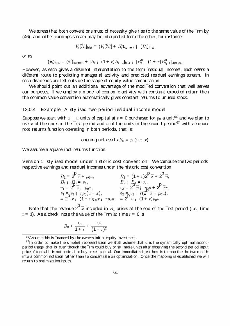
We stress that both conventions must of necessity give rise to the same value of the ¯rm by(46), and either earnings stream may be interpreted from the other, for instance

Vt[fNt]hist = (Vt[fN 0t ] + B0

t)current ¡ (Bt)hist,

or as(evt)hist = (ev0t)current + [Bt ¡ (1 + r)Bt¡1]hist ¡ [B0

t ¡ (1 + r)B0t¡1]current.

However, as each gives a di®erent interpretation to the term `residual income', each o®ers adi®erent route to predicting managerial activity and predicted residual earnings stream. Ineach dividends are left outside the scope of equity-value computation.

We should point out an additional advantage of the modi¯ed convention that well servesour purposes. If we employ a model of economic activity with constant expected return thenthe common value convention automatically gives constant returns to unused stock.

12.0.4 Example: A stylised two period residual income model

Suppose we start with x + u units of capital at t = 0 purchased for p0 a unit66 and we plan touse x of the units in the ¯rst period and u of the units in the second period67 with a squareroot returns function operating in both periods, that is:

opening net assets B0 = p0(u + x).

We assume a square root returns function.

Version 1: stylised model under historic cost convention We compute the two periods'respective earnings and residual incomes under the historic cost convention

B1 = 2p

x + p0u, B2 = (1 + r)2p

x + 2p

u,B1 ¡ B0 = v1, B2 ¡ B1 = v2,v1 = 2

px ¡ p0x, v2 = 2

pu ¡ p0u + 2

pxr,

ev1 = v1 ¡ rp0(u + x), ev2 = v2 ¡ r(2p

x + p0u),= 2

px ¡ (1 + r)p0x ¡ rp0u, = 2

pu ¡ (1 + r)p0u.

Note that the revenue 2p

x included in B1 arises at the end of the ¯rst period (i.e. timet = 1). As a check, note the value of the ¯rm at time t = 0 is

B0 +ev1

1 + r+

ev2(1 + r)2

66Assume this is ¯nanced by the owners initial equity investment.67In order to make the simplest representation we shall assume that u is the dynamically optimal second-

period usage; that is, even though the ¯rm could buy or sell more units after observing the second period inputprice of capital it is not optimal to buy or sell capital. Our immediate object here is to map the the two modelsinto a common notation rather than to concentrate on optimization. Once the mapping is established we willreturn to optimization issues.

61

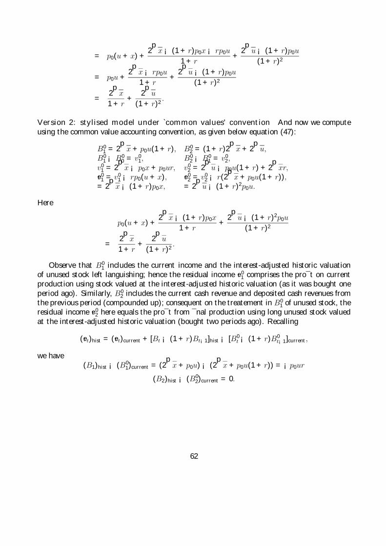
= p0(u + x) +2p

x ¡ (1 + r)p0x ¡ rp0u1 + r

+2p

u ¡ (1 + r)p0u(1 + r)2

= p0u +2p

x ¡ rp0u1 + r

+2p

u ¡ (1 + r)p0u(1 + r)2

=2p

x1 + r

+2p

u(1 + r)2

.

Version 2: stylised model under `common values' convention And now we computeusing the common value accounting convention, as given below equation (47):

B01 = 2

px + p0u(1 + r), B0

2 = (1 + r)2p

x + 2p

u,B0

1 ¡ B00 = v01, B0

2 ¡ B01 = v02,

v01 = 2p

x ¡ p0x + p0ur, v02 = 2p

u ¡ p0u(1 + r) + 2p

xr,ev01 = v01 ¡ rp0(u + x), ev02 = v02 ¡ r(2

px + p0u(1 + r)),

= 2p

x ¡ (1 + r)p0x, = 2p

u ¡ (1 + r)2p0u.

Here

p0(u + x) +2p

x ¡ (1 + r)p0x1 + r

+2p

u ¡ (1 + r)2p0u(1 + r)2

=2p

x1 + r

+2p

u(1 + r)2

.

Observe that B01 includes the current income and the interest-adjusted historic valuation

of unused stock left languishing; hence the residual income ev01 comprises the pro¯t on currentproduction using stock valued at the interest-adjusted historic valuation (as it was bought oneperiod ago). Similarly, B0

2 includes the current cash revenue and deposited cash revenues fromthe previous period (compounded up); consequent on the treatement in B0

1 of unused stock, theresidual income ev02 here equals the pro¯t from ¯nal production using long unused stock valuedat the interest-adjusted historic valuation (bought two periods ago). Recalling

(evt)hist = (evt)current + [Bt ¡ (1 + r)Bt¡1]hist ¡ [B0t ¡ (1 + r)B0

t¡1]current,

we have(B1)hist ¡ (B0

1)current = (2p

x + p0u) ¡ (2p

x + p0u(1 + r)) = ¡p0ur

(B2)hist ¡ (B02)current = 0.

62

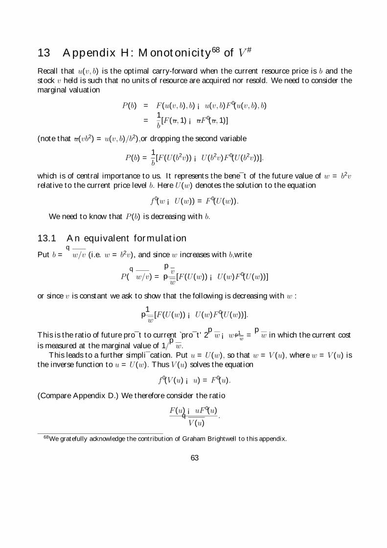
13 Appendix H: Monotonicity68 of V #

Recall that u(v, b) is the optimal carry-forward when the current resource price is b and thestock v held is such that no units of resource are acquired nor resold. We need to consider themarginal valuation

P (b) = F (u(v, b), b) ¡ u(v, b)F 0(u(v, b), b)

=1b[F (~u, 1) ¡ ~uF 0(~u, 1)]

(note that ~u(vb2) = u(v, b)/b2),or dropping the second variable

P (b) =1b[F (U(b2v)) ¡ U(b2v)F 0(U(b2v))].

which is of central importance to us. It represents the bene¯t of the future value of w = b2vrelative to the current price level b. Here U(w) denotes the solution to the equation

f 0(w ¡ U(w)) = F 0(U(w)).

We need to know that P (b) is decreasing with b.

13.1 An equivalent formulation

Put b =q

w/v (i.e. w = b2v), and since w increases with b,write

P (q

w/v) =p

vpw[F (U(w)) ¡ U(w)F 0(U(w))]

or since v is constant we ask to show that the following is decreasing with w :

1pw[F (U(w)) ¡ U(w)F 0(U(w))].

This is the ratio of future pro¯t to current `pro¯t' 2p

w ¡w 1pw =

pw in which the current cost

is measured at the marginal value of 1/p

w.This leads to a further simpli¯cation. Put u = U(w), so that w = V (u), where w = V (u) is

the inverse function to u = U(w). Thus V (u) solves the equation

f 0(V (u) ¡ u) = F 0(u).

(Compare Appendix D.) We therefore consider the ratio

F (u) ¡ uF 0(u)qV (u)

.

68We gratefully acknowledge the contribution of Graham Brightwell to this appendix.

63

13.2 An integral inequalityLet

¦(u) = F (u) ¡ uF 0(u)

=Z 1/

pu

0(1b1

dQ1 +Z 1/(φ1

pu)

1/p

u

pudQ1 +

Z 1

1/(φ1p

u)

1φ1b1

dQ1

we consider¦(u)qV (u)

=¦(u)p

u¢s

uV (u)

.

The left-hand side is an intertemporal comparison of the future use of the apportioned resourceu , against the immediate use of the entire resource V (u). On the right-hand side ¦(u)/

pu

compares the future pro¯t from use of u to the immediate pro¯t from the use of u on its own(which would have led to a bene¯t f#(u) =

pu).

We now let

K(u) = def¦(u)/p

u

=1pu

Z 1/p

u

0

1b1

dQ1 +Z 1/(φ1

pu)

1/p

udQ1 +

1pu

Z 1

1/(φ1p

u)

1φ1b1

dQ1

=1puX + Y

where X = X1 + X2 and

X1 =Z 1/

pu

0

1b1

dQ1, X2 =Z 1

1/(φ1p

u)

1φ1b1

dQ1, Y =Z 1/(φ1

pu)

1/p

udQ1.

Similarly, we may consider the ratio of future marginal bene¯t F 0(u) to the immediate marginalbene¯t of using u namely 1/

pu.We thus put

L(u) = defp

uF 0(u)

=p

uZ 1/

pu

0b1dQ1 +

Z 1/(φp

u)

1/p

udQ1 + φ

pu

Z 1

1/(φp

u)b1dQ1

=p

uZ + Y,

where Z = (Z1 + Z2) and

Z1 =Z 1/

pu

0b1dQ1, Z2 = φ

Z 1

1/(φp

u)b1dQ1

Note that the `apportionment ratio' is

V (u)u

=1u

³u + F 0(u)¡2

´= 1 + L(u)¡2.

64

The ratio of interest is thus

A(u) =defK(u)q

1 + L(u)¡2=

¦(u)pu

¢s

uV (u)

,

and we wish to show A0(u) < 0.As a preliminary we compute that

K 0(u) = ¡12u¡3/2

Z 1/p

u

0

1b1

dQ1 ¡ 12u¡3/2

Z 1

1/(φ1p

u)

1φ1b1

dQ1 < 0,

so that we haveK(u) =

Xpu+ Y, ¡K 0(u) =

X2u3/2 .

LikewiseL0(u) =

12u¡1/2

Z 1/p

u

0b1dQ1 +

12u¡1/2φ

Z 1

1/(φp

u)b1

pudQ1

and again

L(u) =p

uZ + Y, L0(u) =Z

2p

u.

Now

A0(u) =K 0(u)q

1 + L(u)¡2+

K(u)(1 + L(u)¡2)3/2

L0(u)L(u)3

=1

L(u)3 (1 + L(u)¡2)3/2hK 0(u)(L(u)3 + L(u)) + K(u)L0(u)

i

We thus need to show that69

¡K 0(u)(L(u)3 + L(u)) > K(u)L0(u)

or12u¡3/2X

hpuZ + Y + L3

i>

Z2p

u

"Xpu+ Y

#,

i.e.Xu

hpuZ + Y + L3

i> Z

"Xpu+ Y

#.

69Alternatively, we require that

¡K0(u)L(u)3 > K(u)L0(u) + K0(u)L(u)

and the left-hand side is positive. Thus the condition is satis¯ed in any u interval where KL is decreasing in u.

65

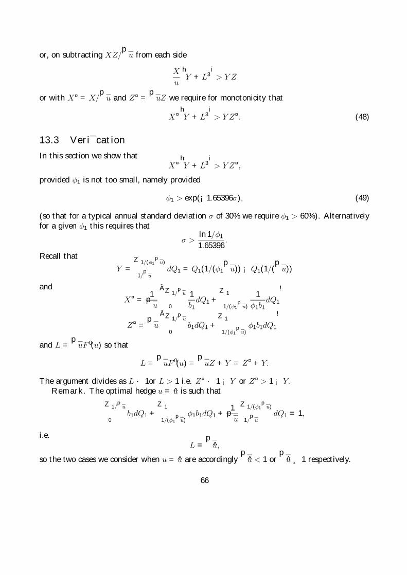
or, on subtracting XZ/p

u from each side

Xu

hY + L3

i> Y Z

or with X¤ = X/p

u and Z¤ =p

uZ we require for monotonicity that

X¤hY + L3

i> Y Z¤. (48)

13.3 Veri¯cationIn this section we show that

X¤hY + L3

i> Y Z¤,

provided φ1 is not too small, namely provided

φ1 > exp(¡1.65396σ), (49)

(so that for a typical annual standard deviation σ of 30% we require φ1 > 60%). Alternativelyfor a given φ1 this requires that

σ >ln 1/φ1

1.65396.

Recall thatY =

Z 1/(φ1p

u)

1/p

udQ1 = Q1(1/(φ1

pu)) ¡ Q1(1/(

pu))

and

X¤ =1pu

ÃZ 1/p

u

0

1b1

dQ1 +Z 1

1/(φ1p

u)

1φ1b1

dQ1

!

Z¤ =p

uÃZ 1/

pu

0b1dQ1 +

Z 1

1/(φ1p

u)φ1b1dQ1

!

and L =p

uF 0(u) so that

L =p

uF 0(u) =p

uZ + Y = Z¤ + Y.

The argument divides as L · 1or L > 1 i.e. Z¤ · 1 ¡ Y or Z¤ > 1 ¡ Y.Remark. The optimal hedge u = u is such that

Z 1/p

u

0b1dQ1 +

Z 1

1/(φ1p

u)φ1b1dQ1 +

1pu

Z 1/(φ1p

u)

1/p

udQ1 = 1,

i.e.L =

pu,

so the two cases we consider when u = u are accordinglyp

u < 1 orp

u ¸ 1 respectively.

66

13.4 Case Z¤ · 1 ¡ Y.i.e. L · 1Now we claim that when L · 1 we have the stronger strict inequality, which evidently implies(48), that

X¤ > Z¤.

Indeed by Jensen's Inequality KL > 1 so if L · 1 then K > 1 ¸ L so in particular

X¤ + Y > Z¤ + Y.

Remark. We have just veri¯ed that in this case

0 > K(u)L0(u) + K 0(u)L(u)

that is KL is decreasing in u.

13.5 Case Z¤ ¸ 1 ¡ Y.i.e. L ¸ 1, or u > 1Here we aim to show that provided

φ1 > exp(¡1.65396σ).

the condition (48) holds.

13.5.1 We prove a tighter condition ...

By Jensen

XZ

=ÃZ 1/

pu

0

1b1

dQ1 +Z 1

1/(φ1p

u)

1φ1b1

dQ1

! ÃZ 1/p

u

0b1dQ1 +

Z 1

1/(φp

u)φb1dQ1

!

> (1 ¡ Y )(1 ¡ Y )

i.e.X¤Z¤ = XZ > (1 ¡ Y )2

To satisfy (48), i.e.X¤(Y + L3) ¸ Y Z¤,

it is equivalent to haveX¤Z¤(Y + L3) ¸ Y (Z¤)2

and thus enough to have(1 ¡ Y )2(Y + L3) > Y (Z¤)2.

67

13.5.2 A monotonicity argument

We consider¢ = (1 ¡ Y )2(Y + [Y + Z¤]3) ¡ Y (Z¤)2

Treating Z¤ as a free variable, so that ¢ = ¢(Z¤), and Y ¯xed at it true value (when u isgiven) observe that this di®erence ¢ is strictly positive (and the strict inequality is true) whenZ¤ = 1 ¡ Y. Indeed

¢(1 ¡ Y ) = (1 ¡ Y )2(Y + 1) ¡ Y (1 ¡ Y )2 = (1 ¡ Y )2.

Recall that L = Z¤ + Y > 1 i.e. Z¤ > 1 ¡ Y. So we check that ¢(Z¤) is increasing in Z¤.We di®erentiate with respect to Z¤ to obtain

¢0 = (1 ¡ Y )2(3 [Y + Z¤]2) ¡ 2Y Z¤.

If(1 ¡ Y )2 >

16

(i.e. Y < 1 ¡ 1/p6,which we term `the

p6 condition') we obtain

¢0 >12[Y + Z¤]2 ¡ 2Y Z¤ ¸ 0,

since[Y + Z¤]2 ¸ 4Y Z¤.

We are now done, i.e. the inequality holds in the case that Z¤ > 1 ¡ Y subject to thep6

condition on Y holding and in fact

¢ > (1 ¡ Y )2 >16. (50)

We now study thep6-condition and show that this is implied by (49).

13.6 Thep6condition

By this we mean

Y = P [φ1t · b1 · t] < 1 ¡ 1p6,

with φ1 < 1 where t = 1/φ1p

u. Now let P1(t) = P [b1 · t] then

P [φ1t · b1 · t] = P1(t) ¡ P1(φ1t)

is easy to study. We haveP1(t) = ©((log t ¡ m)/σ).

68

For t > 0 the function P1(t) ¡ P1(φ1t) has a maximum when

t = em/q

φ1

equal to

1 ¡ 2©(12σ

log φ1),

so that for t > 0 thep6-condition holds uniformly in t provided φ1 is large enough, namely

1 ¡ 2©(12σ

log φ1) < 1 ¡ 1p6

orlog φ1 > 2©¡1(

12p6)σ = ¡1.65396σ

i.e.φ1 > exp(¡1.65396σ).

13.7 N-fold versionIn this section of the appendix we indicate why in the mutiple-period setting it is still true thatprovided φ1 is large enough ¦ is decreasing in price b1 and so V # is increasing in q-income. Oneidenti¯es a condition for monotonicity analogous to that of the two period model and veri¯esthat it holds provided that the forthcoming discount factor φ1 approaches unity. This kind ofargument does not give an explicit bound for φ1 although the condition (49) still needs to hold.The idea of the proof is to demonstrate that the new condition analogous to (48) reduces backto the old condition (48) when we ignore certain terms. As the old condition (48) is a strictinequality and in fact (50) holds, we deduce our result by showing that the additional termstend to zero as φ1 tends to unity. The additional terms contain as factors the two integrals

Z b(v,φ)

b(v)

x(v, b1)/v ¡ x0(v, b1)qx(v, b1)

dQ1,Z b(v,φ)

b(v)

[x(v, b1)/v ¡ x0(v, b1)]x(v, b1)3/2

dQ1.

13.8 Postscript: Monotonicity of y(b)

For the record we prove thaty that y(b) is decreasingWe have since y =

qx(v, b) that

1y= Fu(u(v, b), b) = bFu(~u, 1) = bFu(b2(v ¡ y2), 1)

so¡ 1

y2dydb

= Fu(~u, 1) + bFuu(~u, 1)(2bu ¡ 2yb2dydb

)

69

so Ã2yb3Fuu(~u, 1) ¡ 1

y2

!dydb

= Fu(~u, 1) + Fuu(~u, 1)2~u.

The lhs bracket is negative (since F is concave). So we must now prove the rhs is positive.Here x(u, b1) = u, (in this period no resources can be carried forward), so

Fu(~u, 1) =Z b1(~u)

0b1dQ(b1) + f 0(~u)

Z b1(~u,φ)

b1(~u)dQ(b1) + φ

Z 1

b1(~u,φ)b1dQ(b1)

andFuu(~u, 1) = f 00(~u)

Z b1(~u,φ)

b1(~u)dQ(b1).

But f 0(~u) = ~u1/2, and 2~uf 00(~u) = ¡~u1¡3/2 = ¡~u1/2 thus

Fu(~u, 1) + Fuu(~u, 1)2~u

=Z b1(~u)

0b1dQ(b1) + φ

Z 1

b1(~u,φ)b1dQ(b1)

+[f 0(~u) + 2~uf 00(~u)]Z b1(~u,φ)

b1(~u)dQ(b1)

=Z b1(~u)

0b1dQ(b1) + φ

Z 1

b1(~u,φ)b1dQ(b1) > 0.

70