an analysis method for the correlation between …docs.trb.org/prp/13-0208.pdf1 an analysis method...

Zhang, Qin, Cheng, Jia, Xing 1

An Analysis Method for the Correlation between Catenary Irregularities 1

and Pantograph-catenary Contact Force 2

Yuan Zhang 3

State key laboratory of rail traffic control and safety, Beijing Jiaotong University 4

School of Traffic and Transportation, Beijing Jiaotong University 5

No.3 Shang Yuan Cun, Hai Dian District, Beijing, China 6

Phone: 86-10-51683973 7

Fax: 86-10-51684081 8

Email: [email protected] 9

Yon Qin 10



Phone: 86-10-51683846 13

Fax: 86-10-51683846 14


Xiao-qing Cheng 16



Phone: 86-10-51684081 19

Fax: 86-10-51684081 20


Li-min Jia 22



Phone: 86-10-51683824 25

Fax: 86-10-51683824 26


Zong-yi Xing (corresponding author) 28

School of Mechanical Engineering, Nanjing University of Science and Technology 29

200 Xiao Ling Wei Street, Nanjing, China 30

Phone: 86-10-51683973 31

Fax: 86-10-51684081 32


34

Word count: 4299 35

Figures and Tables: 12 (x 250) 3000 36

Total: 7299 37

38

Submission date: June 26, 201239

TRB 2013 Annual Meeting Paper revised from original submittal.


ABSTRACT 40

Pantograph-catenary contact force provides the main basis for evaluation of current quality collection; however, 41

the pantograph-catenary contact force is largely affected by the catenary irregularities. To analyze the correlated 42

relationship between catenary irregularities and pantograph-catenary contact force, a method based on NARX 43

(Nonlinear Auto-Regressive with eXogenous input) neural networks was developed. First, to collect the test data 44

of catenary irregularities and contact force, the pantograph/catenary dynamics model was established and 45

dynamic simulation was conducted using MATLAB/Simulink. Second, catenary irregularities were used as the 46

input to NARX neural network and the contact force was determined as output of the NARX neural network, in 47

which the neural network was trained by an improved training mechanism based on the regularization algorithm. 48

Third, the simulation results and the comparison with other algorithms indicate the validity and superiority of 49

the proposed approach. 50

Key words: Catenary irregularities; Pantograph-catenary contact force; NARX neural networks; Correlation 51

analysis 52

1 INTRODUCTION 53

With the development of the high-speed railway, electric traction has become the dominant mode providing the 54

train power. It is the key to protecting the safety of running high-speed railways. The EMU (Electric Multiple 55

Units) assure that the current remains in contact with the catenary stably by use of a pantograph-head sliding 56

plate (1, 2). The catenary irregularities are an important cause of current collection performance degradation 57

which may cause impact when the pantograph slips off the catenary. The impact would cause vibration of the 58

pantograph catenary and reduce the current collection performance. The pantograph-catenary contact force is the 59

basic index to measure the quality of current collection, and an inappropriate pantograph-catenary contact force 60

is the main cause of offline pantograph and contact wire fatigue damage (3). In certain operation conditions, 61

pantograph-catenary contact force is influenced by catenary irregularities which would be dominant in high 62

speed, and slight irregularities may cause serious fluctuation of contact force even leading to the pantograph 63

coming off the catenary (4,5). Therefore it is necessary to analyze the relationship of catenary irregularities and 64

pantograph-catenary contact forces. 65

Some scholars studied preliminary correlation analyses concerning the catenary irregularities and 66

pantograph-catenary contact forces. Nagasaka et al (4) designed the measurement and estimation device of 67

catenary irregularities for analyzing the effect on Pantograph-catenary contact force. Han et al (5) analyzed the 68

influence of rigid catenary irregularities on the contact force, and pointed out that the catenary irregularities are 69

the main factors to determine the current collection performance of rigid contact suspension. Takemura et al (6)

70

researched the pantograph vertical vibration which is caused by rigid suspension contact irregularities and 71

proposed the vibration frequency formula. Usuda (7, 8, 9) presented an accurate method to measure the 72

pantograph-catenary contact force, and discussed the relationship between the catenary abrasion and the 73

pantograph-catenary contact force and predicted the abrasion and strain of catenary in high-speed railways. 74

Bennet et al (10) studied the pantograph-catenary contact force detection and a relevant mechanical calculation 75

method. Zhang (11) described the catenary irregularities with full cosine wave, and detected the irregularities 76

which the catenary brings to the contact force in cases of a continuous harmonic wave and a single wave. Xie 77

(12) constructed the pantograph-catenary dynamic model and analyzed the power spectrum of catenary 78

irregularities. All of the above studies focus on the physical detection or impact analysis from single catenary 79



irregularities only, and the research concerning the correlation analysis between catenary irregularities and 80

pantograph-catenary contact force remains at the preliminary qualitative analysis phase, The quantitative 81

correlation analysis between the two is still lacking. 82

The system of catenary irregularities and pantograph-catenary contact force is a typical complex 83

nonlinear dynamic system. Generally it can be described approximately by simplified simultaneous differential 84

equations, but the result has some deviation from the actual system. The neural network can be used to describe 85

any nonlinear system, and has a strong self-learning and fault tolerance ability. For these reasons NARX neural 86

network (13) has been employed to describe the complex dynamic relationship between catenary irregularities 87

and pantograph-catenary contact force. Setting the input of the network are the catenary irregularities and the 88

output is pantograph-catenary force to correlate the analysis of the relationship between them. 89

This paper is organized as follows: section 1 provides some basic descriptions of catenary irregularities 90

and pantograph-catenary contact force, and describes the test data collection methods; section 2 presents NARX 91

neural network, and discusses in detail the regularization algorithm; section 3 conducts the simulation tests 92

based on the method proposed and analyzes the test result; Finally, section 4 makes some conclusions and the 93

direction of future research directions is also given. 94

2 CATENARY IRREGULARITIES AND PANTOGRAPH-CATENARY CONTACT FORCE 95

2.1 Basic Concepts 96

There is no clear common definition or measurement indicator for catenary irregularities. The authors of 97

reference (5) proposed that the rigid catenary irregularities mean that the deviation of the contact surface extends 98

along the current flow with the ideal smooth contact surface, and as a function of the value of the amplitude, 99

divided it into large and small irregularities. Researchers in reference (14) studied the catenary irregularities in 100

elastic suspension mode which is commonly used in high-speed railway , and defined the elastic catenary 101

irregularities both in the broad and narrow sense: The catenary irregularities are the deviation between the actual 102

geometric dimensions and the ideal geometric dimensions of the contact surface, and the definition focuses on 103

researching the influence of catenary abrasive hard spots, hard bend on pantograph vibration and current 104

collection performance; in the broad sense, besides catenary geometric factors, the factors such as the catenary 105

tension, the elastic uniformity, catenary structures, wire material which may cause deviation between the actual 106

contact force and ideal current collection value are also included to define the catenary irregularities. 107

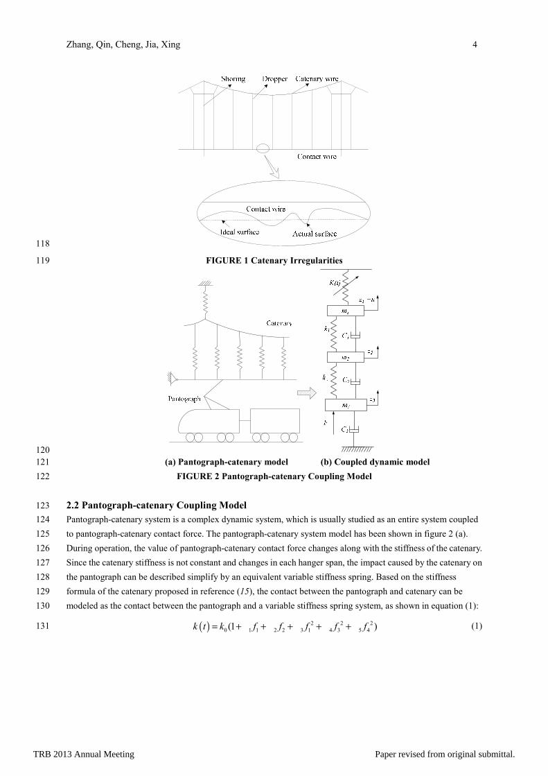
Relative to the above definitions, the influence of slight irregularities on the pantograph-catenary contact 108

force is the only consideration in this paper. It means that in this paper the catenary irregularities are the 109

deviation of the catenary actual geometric state along the tangential direction from the theoretical state which is 110

shown in figure 1. Since the slight catenary irregularities are essentially random processes, the random noises at 111

certain ranges of amplitude have been employed to approximate the irregularities. 112

Pantograph-catenary contact force is the vertical pressure generated during the process as the 113

pantograph rises up to contact the catenary, which also can be interpreted as the uplift force produced by the 114

pantograph. In order to get a stable current performance, the electric locomotive requires a constant pressure 115

between the pantograph and catenary during the operation. However, in actual operation due to the catenary 116

irregularities and aerodynamics, the pantograph-catenary contact force keeps changing constantly. 117



118

FIGURE 1 Catenary Irregularities 119

120

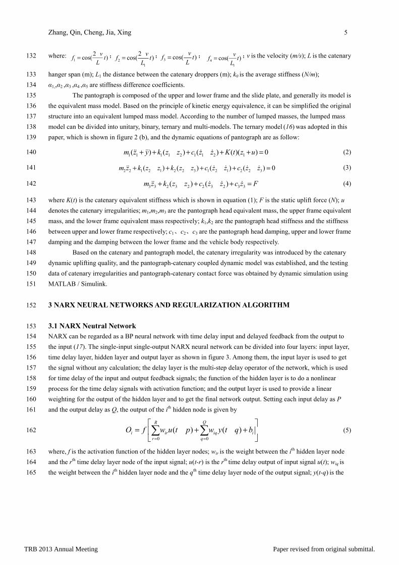
(a) Pantograph-catenary model (b) Coupled dynamic model 121

FIGURE 2 Pantograph-catenary Coupling Model 122

2.2 Pantograph-catenary Coupling Model 123

Pantograph-catenary system is a complex dynamic system, which is usually studied as an entire system coupled 124

to pantograph-catenary contact force. The pantograph-catenary system model has been shown in figure 2 (a). 125

During operation, the value of pantograph-catenary contact force changes along with the stiffness of the catenary. 126

Since the catenary stiffness is not constant and changes in each hanger span, the impact caused by the catenary on 127

the pantograph can be described simplify by an equivalent variable stiffness spring. Based on the stiffness 128

formula of the catenary proposed in reference (15), the contact between the pantograph and catenary can be 129

modeled as the contact between the pantograph and a variable stiffness spring system, as shown in equation (1): 130

( ) 2 2 2

0 1 1 2 2 3 1 4 3 5 4(1 )k t k f f f f fa a a a a= + + + + + (1) 131



where: 1

2cos( )

vf t

L

p= ；2

1

2cos( )

vf t

L

p= ；3 cos( )

vf t

L

p= ； 4

1

cos( )v

f tL

p= ；v is the velocity (m/s); L is the catenary 132

hanger span (m); L1 the distance between the catenary droppers (m); k0 is the average stiffness (N/m); 133

α1,,α2 ,α3 ,α4 ,α5 are stiffness difference coefficients. 134

The pantograph is composed of the upper and lower frame and the slide plate, and generally its model is 135

the equivalent mass model. Based on the principle of kinetic energy equivalence, it can be simplified the original 136

structure into an equivalent lumped mass model. According to the number of lumped masses, the lumped mass 137

model can be divided into unitary, binary, ternary and multi-models. The ternary model (16)

was adopted in this 138

paper, which is shown in figure 2 (b), and the dynamic equations of pantograph are as follow: 139

1 1 1 1 2 1 1 2 1( ) ( ) ( ) ( )( ) 0m z y k z z c z z K t z u+ + - + - + + =ɺɺɺɺ ɺ ɺ

(2) 140

2 2 1 2 1 2 2 3 1 2 1 2 2 3( ) ( ) ( ) ( ) 0m z k z z k z z c z z c z z+ - + - + - + - =ɺɺ ɺ ɺ ɺ ɺ (3) 141

3 3 2 3 2 2 3 2 3 3( ) ( )m z k z z c z z c z F+ - + - + =ɺɺ ɺ ɺ ɺ (4)

142

where K(t) is the catenary equivalent stiffness which is shown in equation (1); F is the static uplift force (N); u 143

denotes the catenary irregularities; m1,m2,m3 are the pantograph head equivalent mass, the upper frame equivalent 144

mass, and the lower frame equivalent mass respectively; k1,k2 are the pantograph head stiffness and the stiffness 145

between upper and lower frame respectively; c1、c2、c3 are the pantograph head damping, upper and lower frame 146

damping and the damping between the lower frame and the vehicle body respectively. 147

Based on the catenary and pantograph model, the catenary irregularity was introduced by the catenary 148

dynamic uplifting quality, and the pantograph-catenary coupled dynamic model was established, and the testing 149

data of catenary irregularities and pantograph-catenary contact force was obtained by dynamic simulation using 150

MATLAB / Simulink.

151

3 NARX NEURAL NETWORKS AND REGULARIZATION ALGORITHM 152

3.1 NARX Neutral Network 153

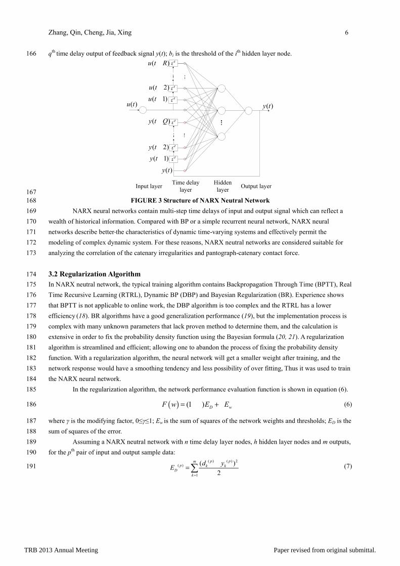
NARX can be regarded as a BP neural network with time delay input and delayed feedback from the output to 154

the input (17). The single-input single-output NARX neural network can be divided into four layers: input layer, 155

time delay layer, hidden layer and output layer as shown in figure 3. Among them, the input layer is used to get 156

the signal without any calculation; the delay layer is the multi-step delay operator of the network, which is used 157

for time delay of the input and output feedback signals; the function of the hidden layer is to do a nonlinear 158

process for the time delay signals with activation function; and the output layer is used to provide a linear 159

weighting for the output of the hidden layer and to get the final network output. Setting each input delay as P 160

and the output delay as Q, the output of the ith

hidden node is given by 161

0 0

( ) ( )Q

i

R

ir iq i

r q

O f w u t p w y t q b= =

= - + - +

∑ ∑ (5) 162

where, f is the activation function of the hidden layer nodes; wir is the weight between the ith

hidden layer node 163

and the rth

time delay layer node of the input signal; u(t-r) is the rth

time delay output of input signal u(t); wiq is 164

the weight between the ith

hidden layer node and the qth

time delay layer node of the output signal; y(t-q) is the 165



qth

time delay output of feedback signal y(t); bi is the threshold of the ith

hidden layer node. 166

z-1

z-1

z-1

( )u t( 1)u t -

( 2)u t -

( )u t R-

( )y t

( 1)y t -

( 2)y t -

( )y t Q-

( )y t

Input layerTime delay

layer

Hidden

layerOutput layer

z-1

z-1

z-1

167

FIGURE 3 Structure of NARX Neutral Network 168

NARX neural networks contain multi-step time delays of input and output signal which can reflect a 169

wealth of historical information. Compared with BP or a simple recurrent neural network, NARX neural 170

networks describe better the characteristics of dynamic time-varying systems and effectively permit the 171

modeling of complex dynamic system. For these reasons, NARX neutral networks are considered suitable for 172

analyzing the correlation of the catenary irregularities and pantograph-catenary contact force. 173

3.2 Regularization Algorithm 174

In NARX neutral network, the typical training algorithm contains Backpropagation Through Time (BPTT), Real 175

Time Recursive Learning (RTRL), Dynamic BP (DBP) and Bayesian Regularization (BR). Experience shows 176

that BPTT is not applicable to online work, the DBP algorithm is too complex and the RTRL has a lower 177

efficiency (18). BR algorithms have a good generalization performance (19), but the implementation process is 178

complex with many unknown parameters that lack proven method to determine them, and the calculation is 179

extensive in order to fix the probability density function using the Bayesian formula (20, 21). A regularization 180

algorithm is streamlined and efficient; allowing one to abandon the process of fixing the probability density 181

function. With a regularization algorithm, the neural network will get a smaller weight after training, and the 182

network response would have a smoothing tendency and less possibility of over fitting, Thus it was used to train 183

the NARX neural network. 184

In the regularization algorithm, the network performance evaluation function is shown in equation (6). 185

( ) (1 ) D wF w E Eg g= - + (6) 186

where γ is the modifying factor, 0≤γ≤1; Ew is the sum of squares of the network weights and thresholds; ED is the 187

sum of squares of the error. 188

Assuming a NARX neutral network with n time delay layer nodes, h hidden layer nodes and m outputs, 189

for the pth

pair of input and output sample data: 190

( ) ( )

1

2( ) ( )

2

p pmp k k

k

D

d yE

=

-=∑ (7) 191



( ) ( )2 2( ) ( )

1 1

)

1

(

1

1[ ]

h n m hp

w

j i k j

p p

ij jk

w

E w wN = = = =

= +∑∑ ∑∑ (8) 192

where dk is the target output of the kth

output layer node; yk is the network output of the kth

output layer node; Nw 193

is the number of the adjustable weight of the neural network; wij is the weight between the ith

time delay layer 194

node and the jth

hidden layer node; wjk is the weight between the jth

hidden layer node and the kth

output layer 195

node. 196

Using the gradient descent method to adjust the weights, and setting the hidden layer activation 197

function 2( ) 1

1h x

f xe l-= -

+ and the output layer transfer function fo(x) = x, and the weight adjustment of the 198

output layer and the hidden layer, the resultant weight adjustments are shown in equations (9) and (10) as. 199

( ) ( ) ( )( ) ( ) ( ) ( 1)21

pp p p p

jk k k Hj jk

w

w d y x wN

g g -D = - × - × + × × (9) 200

( ) ( ) ( ) ( )( ) ( ) ( )( ) ( )

1

21 12

mp p p p p p

ij k k jk H j I i

k

w d y w x xlg

=

D = - - × - ×××∑( 1)2 p

ij

w

wN

g -+ × × (10) 201

Then, the weights of the output layer and the hidden layer after adjusting become 202

( ) ( 1) ( )p p p

jk jk jkw w wh-= - D (11) 203

( ) ( 1) ( )p p p

ij ij ijw w wh-= - D (12) 204

where xHj is the input of the jth

hidden layer node; xIi is the output of the ith

input layer node; η is the learning 205

rate. 206

4 EXPERIMENT AND RESULTS 207

4.1 Data Collection and Processing 208

A typical elastic catenary suspension in China was taken as an illustrative example and the pantograph-catenary 209

coupling dynamic model was simulated by MATLAB / Simulink. The parameters in catenary stiffness equation 210

(1) are v=250km/h, L = 60m, L1=8m, k0 = 1925N/m, α1 = 0.0755, α2 = - 0.0735, α3 = - 0.1459, α4 = - 0.0575, 211

α5=0.0699. The parameters in the pantograph ternary model are F=90N, m1=6.21kg, m2=7 kg, m3=12 kg, 212

k1=2650N/m, k2=10000N/m, c1=100N·s/m, c2=100N·s/m, c3=70N·s/m. Catenary irregularities u result from 213

random noise signal which averages zero and the amplitude range is [－0.5mm to + 0.5mm]. 214

Form the computer simulation model, we have collected 2000 pairs of input and output data at the 215

simulation time of 20s for a sampling frequency of 100Hz. All pairs of the data were separated into two groups: 216

the first group with 1300 pairs of data is employed to train the NARX neutral network and the remaining 700 217

data pairs are used to test the neutral network. To reflect the influence on the pantograph-catenary contact force 218

caused by other factors, a white Gaussian noise of which the amplitude is 5% of the contact force was overlaid. 219

The collected data are shown in figure 4; figure 4(a) portrays the catenary irregularities data and figure 4(b) the 220

pantograph-catenary contact force data. In order to improve the learning efficiency and to speed up the 221

convergence of the neural network, all of the input data and output data were normalized with the following 222

functions. 223



min

max min

scal x xx

x x

-=-

(13) 224

where x, xmax and xmin are the original, the maximum and the minimum values respectively, and xscal

is the value 225

which has been processed. 226

0 2 4 6 8 10 12 14 16 18 20-0.5

0

0.5

(a) Inputs：catenary irregularities time / s

Catenary irregularities / mm

0 2 4 6 8 10 12 14 16 18 20

60

80

100

120

(b) Outputs：pantograph-catenary contact forcestime / s

Pantograph-catenary

contact forces / N

227

FIGURE 4 Inputs and Outputs Data 228

4.2 Correlation Analysis 229

To evaluate the performance of the obtained neural network, the RMSE (Root Mean Square Error) which has 230

been shown in equation (14) is employed to represent the precision of the obtained network. The network has a 231

higher accuracy as the RMSE decreases. However, since the values of RMSE are generally small, it is difficult 232

to evaluate the network performance visually, so the correlation coefficient R is introduced to assess the 233

correlation between the target outputs and the neural network outputs which are shown in equation (15). When 234

R is closer to 1, it shows the model would have a better accuracy and will be more similar to the actual system. 235

( ) ( ) ( ) 2

1

1, ( )

N

m M

l

RMSE y y y yN

l l=

= -∑ (14) 236

( )2

1

1

2

1

( )( )

,

( ) ( )

l

l

N

l

l

N N

l

M M

m

Ml

l

M

y y y y

R y y

y y y y

=

= =

- -=

- -

∑

∑ ∑

(15) 237

where, y is the target outputs, yM is the neural network outputs; N is the number of the data samples; y and 238

My are the averages of the y and yM samples, respectively. 239

First of all, to indicate the complex relationship between the catenary irregularities and the 240

Pantograph-catenary contact force, the experiment was carried out based on the BP neural network with the 241

Levenberg-Marquardt (LM) algorithm and the result is shown in TABLE 1. The training and the testing RMES 242

of the BP neural network are 0.1393 and 0.2401 respectively and the correlation coefficient R is 0.4274 and 243

0.1845 respectively. At the same time, figure 5 shows the comparison of the target outputs and the BP neural 244



network output. Among them, figure 5(a) shows the comparison of the training data samples while figure 5(b) 245

shows the comparison of the testing data samples. It can be seen that the BP neutral network cannot describe the 246

complex relationship between the catenary irregularities and the pantograph-catenary contact force. 247

TABLE 1 the Performance Index of Each Model 248

Models→

Indexes↓ BP Elman-LM NARX-R

Training RMSE 0.1393 0.1089 0.0533

Testing RMSE 0.2401 0.1189 0.1100

Training R 0.4274 0.7058 0.9384

Testing R 0.1845 0.6988 0.8029

0 200 400 600 800 1000 1200

0

0.5

1

Number of training samples

Norm

alized contact forces

(a) Outputs contrast of training samples

0 100 200 300 400 500 600 700

0

0.5

1

Number of testing samples

Norm


(b) Outputs contrast of testing samples

Target outputs Neural network outputs


y(l)

249

FIGURE 5 Comparisons of the Target Outputs and the BP Neutral Network Outputs 250

In order to demonstrate the effectiveness of the NARX neural network, both the NARX neural network 251

with a regularization algorithm (referred to as NARX-R) and the Elman neural network with the LM algorithm 252

(referred to as Elman-LM) were implemented. Based on the expert experience and trial and error method, for 253

NARX-R, the number of input and output delay steps was determined as 45 and the number of hidden layer 254

nodes was set to 17. With the Elman-LM, the number of hidden layer nodes was set at 20. 255

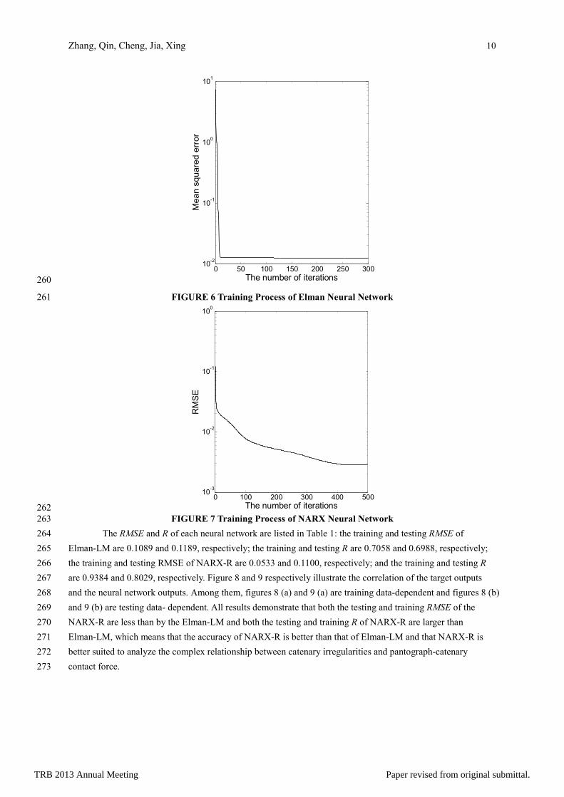
Figure 6 shows the curve of mean-squared training error using the iterative process of Elman-LM. 256

After 300 epochs training, the training error became stable. Figure 7 shows the training RMSE of NARX-R 257

changes with the iterations, which shows that the error was no longer reduced after 450 epochs. Therefore, the 258

number of iterations of Elman-LM and NARX-R were initialized to 300 and 500 respectively. 259



0 50 100 150 200 250 30010

-2

10-1

100

101

The number of iterations

Mean squared error

260

FIGURE 6 Training Process of Elman Neural Network 261

0 100 200 300 400 50010

-3

10-2

10-1

100

The number of iterations

RMSE

262

FIGURE 7 Training Process of NARX Neural Network 263

The RMSE and R of each neural network are listed in Table 1: the training and testing RMSE of 264

Elman-LM are 0.1089 and 0.1189, respectively; the training and testing R are 0.7058 and 0.6988, respectively; 265

the training and testing RMSE of NARX-R are 0.0533 and 0.1100, respectively; and the training and testing R 266

are 0.9384 and 0.8029, respectively. Figure 8 and 9 respectively illustrate the correlation of the target outputs 267

and the neural network outputs. Among them, figures 8 (a) and 9 (a) are training data-dependent and figures 8 (b) 268

and 9 (b) are testing data- dependent. All results demonstrate that both the testing and training RMSE of the 269

NARX-R are less than by the Elman-LM and both the testing and training R of NARX-R are larger than 270

Elman-LM, which means that the accuracy of NARX-R is better than that of Elman-LM and that NARX-R is 271

better suited to analyze the complex relationship between catenary irregularities and pantograph-catenary 272

contact force. 273



0 0.2 0.4 0.6 0.8 10

0.1

0.2

0.3

0.4

0.5

0.6

0.7

0.8

0.9

1

Targets T

Outputs Y, Linear Fit: Y=(0.5)T+(0.26)

Outputs vs. Targets, R=0.70583

Data Points

Best Linear Fit

Y = T

0 0.2 0.4 0.6 0.8 10

0.1

0.2

0.3

0.4

0.5

0.6

0.7

0.8

0.9

1

Targets T

Outputs Y, Linear Fit: Y=(0.62)T+(0.21)


Data Points

Best Linear Fit

Y = T

274

(a) Correlation of training data (b) Correlation of testing data 275

FIGURE 8 Correlation Analysis of the Target Outputs and Elman Neural Network Outputs 276

0 0.2 0.4 0.6 0.8 10

0.1

0.2

0.3

0.4

0.5

0.6

0.7

0.8

0.9

1

Targets T

Outputs A, Linear Fit: A=(0.85)T+(0.08)


Data Points

Best Linear Fit

A = T

0 0.2 0.4 0.6 0.8 10

0.1

0.2

0.3

0.4

0.5

0.6

0.7

0.8

0.9

1

Targets T

Outputs A, Linear Fit: A=(0.8)T+(0.14)


Data Points

Best Linear Fit

A = T

277

(a) Correlation of training data (b) Correlation of testing data 278

FIGURE 9 Correlation Analysis of the Target Outputs and NARX Neural Network Outputs 279

For delineating the performance of NAEX-R and Elman-LM more directly, the comparisons of the 280

target outputs and the neural network outputs of Elman-LM and NARX-R are shown in figures 10 and 11 in 281

which figures 10(a) and 11(a) are for the training data, and figures 10(b) and 11(b) are for the testing data. It is 282

thus clear that comparing with Elman-LM, the neural network outputs of NARX-R displays a better conformity 283

with the target outputs and can follow the tendency of the target outputs better. 284

In summary, the NARX-R method proposed in this paper can fit the characteristics of the complex 285

dynamic system better, and accurately achieve the correlation analysis of the catenary irregularities and 286

pantograph-catenary contact force. 287



0 200 400 600 800 1000 1200 1400

0

0.5

1


Norm




0 100 200 300 400 500 600 700

0

0.5

1


Norm




288

FIGURE 10 Comparisons of the Target Outputs and Elman Neural Network Outputs 289

0 200 400 600 800 1000 1200

0

0.5

1


Norm



0 100 200 300 400 500 600 700

0

0.5

1


Norm





290

FIGURE 11 Comparisons of the Target Outputs and NARX Neural Network Outputs 291

5 CONCLUSIONS 292

Based on the NARX neural network, a correlation analysis method is developed to analyze the complex 293

dynamic relation between the catenary irregularities and the pantograph-catenary contact force. In order to train 294

the NARX neural network, a pantograph-catenary coupling dynamic model is constructed to obtain the 295

experimental data of catenary irregularities and pantograph-catenary contact force and a regularization 296

algorithm is adopted. The simulation results and comparisons with other neural networks demonstrate the 297

effectiveness and validity of the proposed method. Further research efforts will be made toward including other 298

kinds of catenary irregularities and improvements of the structure of the NARX neural network and optimization 299

of the algorithm to enhance network performance. In addition, the experimental data collected in this paper is 300



obtained by using computer simulation model, so the real measurements of catenary irregularities and the 301

pantograph-catenary contact force will be needed to further verify the validity and improve the applicability of 302

the method. 303

ACKNOWLEDGEMENT 304

This research was sponsored by National Key Technology R&D Program of China (No. 2011BAG01B05) and 305

National High-tech R&D Program of China (863 Program, No. 2011AA110501) and the State Key Laboratory 306

of Rail Traffic Control and Safety (No. RCS2010ZZ002) of Beijing Jiaotong University. Their supports are 307

gratefully acknowledged. 308

REFERENCE 309

(1) A. Facchinetti, S. Bruni. Hardware-in-the-loop hybrid simulation of pantograph–catenary interaction. 310

Journal of Sound and Vibration, Vol. 331, No. 12, 2012, pp. 2783-2797. 311

(2) G. Poetsch, J. Evans, R. Meisinger, W. Kortüm, W. Baldauf, A. Veitl, J. Wallaschek. Pantograph/catenary 312

dynamics and control， Vehicle System Dynamics, Vol. 28, No. 2-3, 1997, pp. 159-195. 313

(3) K. Lee. Analysis of dynamic contact between overhead wire and pantograph of a high-speed electric train. 314

Proceedings of the Institution of Mechanical Engineers, Part F: Journal of Rail and Rapid Transit, Vol.221, 315

No. 2, 2007, pp. 157-166. 316

(4) S. Nagasaka, M. Aboshi. Measurement and Estimation of Contact Wire Unevenness. Quarterly Report of 317

RTRI, Vol.45, No. 2, 2004, pp. 86-91. 318

(5) Z. X. Han, G. L. Wang. Unevenness Analysis of Overhead Rigid Suspension Catenary. Journal of Railway 319

Engineering Society, No. 2, 2007, pp. 61-64. (In Chinese) 320

(6) T. Takemura, Y. Fujii, M. Shimizu. Characteristics of over-head rigid conductor line having T-type cross 321

section. Developments in Mass Transit Systems, Vol. 4, 1998, pp. 173-177. 322

(7) T. Usuda. The Pantograph Contact Force Measurement Method in Overhead Catenary System. World 323

Congress on Railway Research, 2008. http://www.uic.org/cdrom/2008/11_wcrr2008/pdf/S.1.4.3.4.pdf. 324

Accessed September 9, 2011 325

(8) T. Usuda. Prediction of Contact Wire on High-speed Railways. Railway Technology Avalanche. Vol. 36, 326

2011, pp.214. 327

(9) T. Usuda. Estimation of Wear and Strain of Contact Wire Using Contact Force of Pantograph. Quarterly 328

Report of RTRI. Vol.48, No. 3, 2007, pp.170-175. 329

(10) Bennet, J., Montesinos, J., Cuartero, F., Rojo, T. Arias. E Advanced Algorithm to Calculate Mechanical 330

Forces on a Catenary. Computers in Railways IX, 2009, pp.857-868. 331

(11) W. H. Zhang, G. M. Mei, L. Q. Chen. Analysis of the influence of catenary’s sag and irregularity upon the 332

quality of current-feeding. Journal of the China railway Society. Vol. 22, No. 6, 2000, pp. 50-54. (In 333

Chinese) 334

(12) J. Xie, Z. G. Liu, Z. W. Han. Pantograph and Overhead Contact Line Coupling Dynamic Model Simulation 335

and Analysis of Imbalance of Overhead Contact Line. Electric Railway, No. 6, 2009, pp. 23-26,29. (In 336

Chinese) 337

(13) Siegelmann H. T. Computational capabilities of recurrent NARX neural networks. IEEE Transactions on 338

Systems, Man, and Cybernetics, Part B: Cybernetics, Vol. 27, No. 2, 1997, pp. 208-215. 339



(14) Z. G. Liu, Z. W. Han. Power Spectrum Research of Catenary Irregularities of Electrified Railway. Electric 340

Railway. No. 1, 2011, pp. 1-3. (In Chinese) 341

(15) J. B. Guo. Stability of Current Collection and Control for High-Speed Locomotive. Beijing. PhD thesis. 342

Beijing Jiaotong University. 2006. (In Chinese) 343

(16) T. X. Wu, M. J. Brennan. Dynamic stiffness of a railway overhead wires system and its effect on 344

pantograph-catenary system dynamics. Journal of Sound and Vibration, Vol. 3, 1999, pp. 483-502. 345

(17) S. Haykin. Neural Networks: A Comprehensive Foundation. 2nd ed. Prentice-Hall Inc., New Jersey, 1999. 346

(18) Y. Q. Liu, G. F. Ma, Z. Shi. NARX network for dynamic system identification in adaptive inverse control. 347

Journal of Harbin Institute of Technology. Vol. 37, No. 2, 2005, pp. 173-176. (In Chinese) 348

(19) Sumit, G., Gyanendra, K. G. Time – Delay Simulated Artificial Neural Network Models for Predicting 349

Shelf Life of Processed Cheese. International Journal of Intelligent Systems and Applications, Vol.4, No.5, 350

2012, pp. 30-37. 351

(20) P. Kumar, S. N. Merchant, U. B. Desai. Improving performance in pulse radar detection using Bayesian 352

regularization for neural network training. Digital signal processing, Vol. 14, 2004, pp. 438-448. 353

(21) K. Hirschen, M. Schafer. Bayesian regularization neural networks for optimizing fluid flow processes. 354

Computer methods in applied mechanics and engineering, Vol. 195, 2006, pp.481-500. 355


an analysis method for the correlation between …docs.trb.org/prp/13-0208.pdf1 an analysis method...

Documents