an analysis of a superconvergence result for a singularly ...€¦mathematics of computation volume...
TRANSCRIPT

MATHEMATICS OF COMPUTATIONVOLUME 46. NUMBER 173JANUARY 19X6. PAC'iES 81-92
An Analysis of a Superconvergence Result
for a Singularly Perturbed
Boundary Value Problem*
By Eugene O'Riordan and Martin Stynes
Abstract. We give a new proof that the El-Mistikawy and Werle finite-difference scheme is
uniformly second-order accurate for a nonselfadjoint singularly perturbed boundary value
problem. To do this, we use exponential finite elements and a discretized Green's function.
The proof is direct, gives the nodal errors explicitly in integral form, and involves much less
computation than in previous proofs of the result.
1. Introduction. In this paper we consider the nonselfadjoint singularly perturbed
boundary value problem
Lu = eu" + au' = / on (0,1),
V ' ' u(0) = u0, u(l) = ux,
where the functions a and / are in C2[0,1], a(x) > a > 0 on [0,1], e is a parameter
in (0,1], a and / do not depend on e, and u0, ux are fixed constants. Under these
assumptions, (1.1) has a unique solution u(x). This solution has, in general, a
boundary layer at x = 0 for e near 0.
A difference scheme for solving (1.1) on a uniform mesh in [0,1] was proposed in
El-Mistikawy and Werle [2]. In Berger et al. [1] and Hegarty et al. [4] two
independent proofs were given that the El-Mistikawy and Werle scheme was
uniformly second-order accurate (that is, all nodal errors are bounded by Ch2, where
the constant C is independent of x, h and e). Although these proofs differ greatly in
their details, both use finite-difference techniques and involve large amounts of
computation and estimation.
We give below a new proof of the uniform second-order accuracy of the El-Mis-
tikawy and Werle scheme. An outline of the proof was given in Stynes and
O'Riordan [11]. It has previously been shown by O'Riordan [8], [9] that a certain
choice of finite elements together with a nonstandard quadrature rule generate the
scheme. Thus the problem of proving the accuracy of the scheme can be approached
from a finite-element viewpoint. The key to the proof is the introduction of a
"discretized Green's function" associated with a modified version of (1.1), obtained
by replacing the functions a and / by piecewise constant approximations. The nodal
errors are then easily expressed explicitly as integrals involving the discretized
Received June 28, 1984; revised March 5, 1985.
1980 Mathematics Subject Classification. Primary 65L10; Secondary 34B27, 34E15.
This paper was written while both authors were at Waterford Regional Technical College, Waterford,
Ireland.
©1986 American Mathematical Society
0025-5718/86 $1.00 + $.25 per page
81
License or copyright restrictions may apply to redistribution; see https://www.ams.org/journal-terms-of-use
82 EUGENE O'RIORDAN AND MARTIN STYNES
Green's function (see Section 4). Most of these integrals are seen almost immediately
to be bounded by Ch2, and we are left with the problem of estimating a single
integral involving the boundary-layer term from an asymptotic expansion of u.
Some computation is necessary to bound this integral, but it is very much less than
the difficulties involved in the finite-difference proofs of the result.
With a natural choice of trial functions the Petrov-Galerkin finite-element method
used here is globally uniformly first-order accurate, as shown in O'Riordan [8], [9].
Thus the bound proven here is a superconvergence result.
The discretized Green's function technique can readily be applied to other
singularly perturbed problems. In [12] we use it to prove that a certain difference
scheme is uniformly second-order accurate for a conservative nonselfadjoint singu-
larly perturbed two-point boundary value problem. In fact, as may be seen in [12],
the discretized Green's function actually suggests (indirectly) a good choice of
difference scheme for this problem.
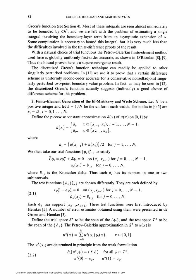
2. Finite-Element Generation of the El-Mistikawy and Werle Scheme. Let TV be a
positive integer and let h = 1/N be the uniform mesh width. The nodes in [0,1] are
x¡ = ih, i = 0,1, ...,7V.
Define the piecewise constant approximation a(x) of a(x) on [0,1] by
/«a,, x G [*,_,,*,), i = 1,...,7V- 1,a(x)=(_ r x
\ flyv' X L-*iV-l' XN1>
where
Sj = {a(xJ_1) + a(Xj))/2 tor j = 1,...,7V.
We then take our trial functions {<¿>,}¡L0 t0 satisfy
L<t>, = etf + ati = 0 on (Xj, xJ+x) for j = 0,..., TV - 1,
<¡>¡(xJ) = 8iJ forj = 0,...,N,
where S, ¡ is the Kronecker delta. Thus each <b¡ has its support in one or two
subintervals.
The test functions {ipk }kZ¡ are chosen differently. They are each defined by
8*i'- a*i - 0 on(Xj,xJ+x)forj = 0,...,N-l,
**(*>)-**., for; = 0,..., TV.
Each \j/k has support [xk_x,xk + x\. These test functions were first introduced by
Hemker [5]. A number of error estimates obtained using them were presented in de
Groen and Hemker [3].
Define the trial space Sh to be the span of the {</>,-}, and the test space Th to be
the span of the {\pk}. The Petrov-Galerkin approximation in 5* to u(x) is
«*(*)-£ «*(*,)*(*), *e[0,l].f-0
The uh(x¡) are determined in principle from the weak formulation
«,(«*,*)-(/,*) forall^er*,
uh(0) = uo, uh(l) = ux,
License or copyright restrictions may apply to redistribution; see https://www.ams.org/journal-terms-of-use

SINGULARLY PERTURBED BOUNDARY VALUE PROBLEM 83
where
Be(v,w) = (v',-ew' + aw), v,we HX(0,1),
and
(v,w) = / v(x)w(x) dx, v, w e L2(0,1).Jo
However, the integrals in (2.2) cannot in general be evaluated exactly, so some
quadrature rule must be employed. Following O'Riordan [9] we replace the func-
tions a and / by ä and / respectively, where / is defined analogously to a. The
integrals can then be evaluated exactly. We now have an approximation üh(x) e Sh
to u(x) with
N
ü"(x)=Ziüh(xi)4>i(x), xe[0,l].i = 0
The üh(x¡) are determined from
(23) *.(ö\*)-(/» for all* G 7",
ûh(0) = u0, ûh(l) = ux,
where
Be(v,w) = (v',-ew' + äw), v, w e Hx(0,l).
On evaluating (2.3) explicitly, one obtains the El-Mistikawy and Werle difference
scheme for the Uh(xi), as shown in O'Riordan [8], [9]. This calculation is easy but
tedious, so we do not reproduce it here. It is interesting to note that the difference
scheme generated does not depend on the specific choice of <j>¡ made above; one
merely needs the usual trial function properties that each <¡>¡ has support [x,_x,xi+x]
with <¡>,(Xj) = 8,j.
For our choice of Sh and Th, it is shown in O'Riordan [9] that \\u — üh\\x < Ch
(here and throughout the paper C denotes a generic constant independent of x, h
and e). Thus, the bound we prove below, that
max \u(x¡) - üh(x¡) I < Ch2,omaN
is a superconvergence result.
3. Discretized Green's Function. For each j'e {1,...,7V— 1} we define a dis-
cretized Green's function G . Formally it satisfies
L^x) - eG'/(x) -(ä(x)Gj(x))' = 8(x - *,), G,(0) = G,(l) = 0,
where ô(-) is the Dirac 5-distribution.
More precisely, Gy is defined by
(3.1a) G,eC [0,1],
(3.1b) G,(0) = G,(l) = 0,
(3.1c) G" exists and is continuous on [0,1] , where [0,1]
denotes [O,!]^*!,...,*^,},
(3.Id) eGj" - äGj = 0 on [0,1 ] ",
(3.1e) Um (eu/ - äGj) - lim+ (eG/ - dGj) = -8tJ for i = 1,..., N - 1.
License or copyright restrictions may apply to redistribution; see https://www.ams.org/journal-terms-of-use

84 EUGENE O'RIORDAN AND MARTIN STYNES
Remark. (3.1e) is equivalent to
id on[0,x,)n[0,l]\(3.2) eG'(x) - a(x)G,(x) = { '. ! ,.V ' A ' ' A \d+l on(jc,,l]n[0,l] ,
where d = d(j,h, e). Setting x = 0 gives d = eGj(0).
Notation. pa = ah/e, p, = 5¡h/e for i = 1,..., N.
We note that Lemmas 3.1 and 3.2 are in fact valid for any choice of ä: ^ a,
/ = 1,...,7V.
Lemma 3.1. G, e Th.
Proof. We must show that constants ak can be chosen such that
N-l
Gj = E «***■k = l
Clearly, (3.1a), (3.1b), (3.1c) and (3.Id) are satisfied for any choice of {ak}. Using
integration by parts on [jei_1,jci] and [x¡, xi+x] to evaluate Be(^>¡, G¡), one sees from
(3.le) that the {ak} must satisfy
JV-l
(3.3) E akBt(^^k) = StJ for i = 1,..., N-l.k = l
But (2.3) may be written as
Ar-i
(3.4) E üh(x,)Be(<t>^k) = (/>,) for* = l,...,7V-l.¡-1
Hence, the matrix of the Unear system of equations (3.3) is the transpose of the
matrix of the linear system (3.4). This latter matrix is the matrix of the El-Mistikawy
and Werle difference scheme, which is well known to be invertible (see, e.g., Berger
et al. [1]). Consequently the matrix of (3.3) is invertible, and we are done.
Lemma 3.2. Let A(x) = \q a(t) dtfor 0 < x < 1. Then
(i)
Gj(x)
(ü)
de 1exp(^4(x)/e) Í exp(-vi(r)/e) dt, 0 < x < Xj,
-(d + l)e~xexp(A(x)/e) j exp(-^4(i)/e) dt, Xj < x < 1.
- H exp(-A(t)/e) dtd
fxexp(-A(t)/e) dt
(iii) Gj < 0 on (0,1).
(iv) Gj is strictly decreasing on [0, xA.
(v) Gj > -I/o on [0,1].
Proof. Multiplying (3.2) by the integrating factor e_1exp(-yl(jc)/e) and in-
tegrating from 0 to x (for x < Xj) or from x to 1 (for x ^ xj) yields (i).
Equating the two formulas of (i) at x = x¡ gives (ii).
From (ii), -1 < d < 0, and then (i) yields (iii) immediately.
License or copyright restrictions may apply to redistribution; see https://www.ams.org/journal-terms-of-use

SINGULARLY PERTURBED BOUNDARY VALUE PROBLEM 85
Note that (Gj(x)exp(-Ä(x)/e))' = de'xtxp(-Ä(x)/e) on [0,Xj] n [0,1]". Hence,
Gj(x)txp(-A(x)/e) is strictly decreasing on [0, *■]. But on (0, Xj), Gy < 0 and
exp(-A(x)/e) > 0 is strictly decreasing. This implies (iv).
For (v) suppose that Gj(z) < -1/a, where z e [X/_i, x¡] for some /'. Then (with
appropriate modifications if z is a node)
<c«-.yw.)+{í+1 ;;;>■< í/ (by choice of z )
<0.
It follows that Gj is strictly decreasing on [z, x¡]. Hence, G/x,) < -1/a, and the
above argument can be repeated on successive intervals until we obtain G/l) < -1/a,
contradicting G/l) = 0.
The next lemma is a technical result needed only to prove Lemma 3.4. Both of
these lemmas remain valid for any choice of ä satisfying 5, > a and \a¡ - 5,_,| < Ch,
i = l,...,7V.
Lemma 3.3. For j < / < TV,
/ N-i-l \
|äfG,.(jcf.) + </+ l|< C exp(-(7V - i)pj + A E exp(-*pa) .\ fc-o /
Proof. For _/ < / < TV,
eGj'(x) - a¡Gj(x) = d + 1 on (*,_!, .x,).
Thus,
(3.5) (GJ(x)exp(-5ix/e))' = e'x(d + l)exp(-a,x/e) on (*,_,,*,)•
Integrating this from x — x^x to x = x¡ and dividing by exp(-â,x,_1/e) yields
(3.6) G,.U)exp(-p,) - Gj(x,.x) = (d + l)(l - exp(-p,))/,5,.
We now use induction on ;' to prove the lemma.
For /' = TV the lemma holds since \d + 1| < 1 by Lemma 3.2(h).
Assume that the lemma holds for some i with j < i < TV. We deduce that it also
holds for í — 1 :
*,-iGj(*i-i) + d+l = (a,_x - afjG^x,.,) + Sfijix,^) + d + 1
= 0,-1 - ä,)C,U-i) + («,<?,(*,) + d+ l)exp(-p,), by (3.6).
By the inductive hypothesis and Lemma 3.2, parts (iii) and (v)
k-iG;U-i) + ¿+l|
< C A + exp(-pj exp(-(TV - z)p„) + fi ¿ exp(-*pj
= C exp(-(TV - i + l)Pa) + h E exp(-*p0) ,
as required.
License or copyright restrictions may apply to redistribution; see https://www.ams.org/journal-terms-of-use
86 EUGENE O'RIORDAN AND MARTIN STYNES
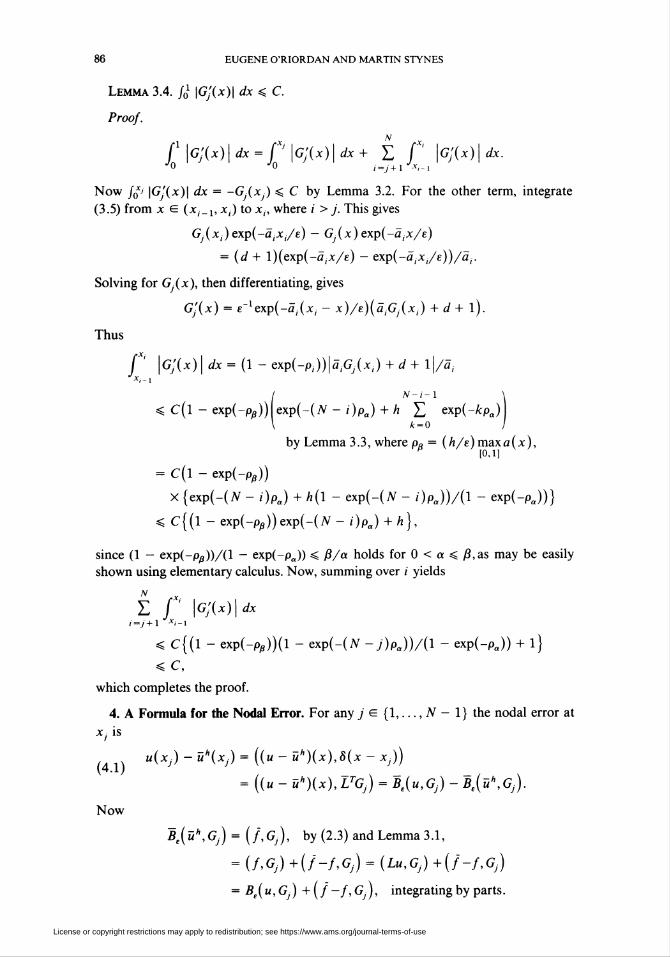
n \r>iLemma 3.4. j¿ \Gj(x)\ dx < C.
Proof.
x N X
f \g'(x)\ dx = f J \G'(x)\ dx + E (" \GJ(x)\dx.
Now JqJ \Gj'(x)\ dx = -Gj(xj) < C by Lemma 3.2. For the other term, integrate
(3.5) from x e (xt_x, x¡) to x¡, where /' > j. This gives
G,(x,)exp(-â,oc,/e) - GJ(x)exp(-äix/e)
= (d + l)(exp(-ä,V<0 - exp(-aiXj/e))/a¡.
Solving for Gj(x), then differentiating, gives
G'j(x) = e-xexp(-ä,(x, - x)/e){âiGJ(xl) + d+l).
Thus
f" \Gj(x) \dx=(l- exp(-p,))|â,G7(x,) + d + l\/-a,
< C(l - exp(-Pj3)) exp(-(TV - i)Pa) + h ¿ exp(-APa)
by Lemma 3.3, where pß = (h/e)maxa(x),[0,1]
= C(l - exp(-p^))
X {exp(-(TV - i)Pa) + h(l - exp(-(TV - f)p.))/(l - exp(-pj)}
< C{(1 - exp(-P/J))exp(-(TV - i)Pa)+h),
since (1 - exp(-p£))/(l - exp(-pj) «s ß/a holds for 0 < a < ß,as may be easily
shown using elementary calculus. Now, summing over / yields
e r \G¡(x)\dx
« C{(l - exp(-P/?))(l - exp(-(TV -j)Pa))/(l - exp(-pj) + l}
< C,
which completes the proof.
4. A Formula for the Nodal Error. For any j e {1,..., TV - 1} the nodal error at
Xj is
u(xJ)-W(xJ) = {(u-üh)(x),8(x-xJ))
= ((« - B*)(*),FG,) = *e(«,G,) - 5.(«\G,).
Now
Bt(ü",Gj) = (f,Gj), by (2.3) and Lemma 3.1,
= (f,Gj) +(f'-f,Gj) = (Lu,Gj) +{f-f,Gj)
= Be(u,Gj) +(f-f,Gj), integrating by parts.
License or copyright restrictions may apply to redistribution; see https://www.ams.org/journal-terms-of-use

SINGULARLY PERTURBED BOUNDARY VALUE PROBLEM 87
Hence, (4.1) becomes
(42) u(xj) - üh(Xj) = BA^Gj) - Äe(u,G,) +{f-f,GJ)
= {u',(â-a)Gj)+(f-f,Gj).
5. Estimation of the Nodal Error. Our approach here is to replace u in the
right-hand side of (4.2) by an asymptotic expansion. Each of the resulting terms is
then shown to be bounded by Ch2.
Lemma 5.1. Let r G C2[0,1] be independent of e. Let jeC[0,l] with s G
C1(xi,xi+X) for each i and /0V(OI dt defined. Define f (piecewise constant ap-
proximation of r) on [0,1] analogously to the definitions ofä andf. Then
|(r-f,j)|< Ch2l\s(l)\ + f1 \s'(t)\ dt
Proof. For 0 < x < 1 set R(x) = /0X r(t) dt, R(x) = j¿ r(t) dt. Then the classi-
cal error estimate for the trapezoidal rule gives
|a(x,)-ÍR(x,)|< Ch2Xi for i = 0,..., TV.
For any x in [0,1] we have x g [x¡, xl + x] for some i. Hence,
|ä(jc)-.R(jc)| = R(x,) - R(x,) - f (-r(t) - r(t)) dt
^Ch2x: + Ch2, as |r-r|< Ch,
< Ch2.
Thus, integrating by parts,
\(r - -r,s)\= (R(l) -R(l))s(l) - f (R(t) -R(t))s'(t) dt
<Ch2l\s(l)\ + f \s'(t)\dt\.0
2COROLLARY 5.2. If - f,Gj)\ < Ch2.
Proof. Use Lemma 3.4.
Notation. O(h') denotes a quantity whose absolute value is bounded by Ch',
i = 0,1,2.
Applying Corollary 5.2 to (4.2) gives
(5.1) u(xj) - «*(*,) = («',(* - a)Gj) + 0(h2).
Lemma 5.3 (Berger et al. [1, Lemma 3.2], Smith [10]).
(5.2) u(x) = B0(x) + C(a(x))'lexp(-A(x)/e) + eR0(x),
where B0 is smooth and independent of e, and A(x) = /0X a(t) dt for 0 < x < 1. The
function R0 satisfies
LR0(x) = F0(x,e) on (0,1),
Ro(0) = 0, jR0(1) = Vo(e),
where for e G (0,1], |y0(e)| < C and |JF0(jc, e)| < C for 0 < x < 1.
License or copyright restrictions may apply to redistribution; see https://www.ams.org/journal-terms-of-use

88 EUGENE O'RIORDAN AND MARTIN STYNES
Remark. By Kellogg and Tsan [7],
(5.3) Ia^Íjc)!* C(l + e-'expí-Cjje/i!)) forO < x < 1, i - 0,1,
where Cx > 0 is a constant independent of x, h and e. Hence /J |eÄ'0'(x)| í/x =
/o1 |-a(Jc)Ä'0(jc) + F0(x, e)| < C.
From Lemma 5.3,
(5.4) u'(x) = -Ce'lexp(-A(x)/e) + J(x),
where
J(x) = B^(x) + eR'0(x) - Ca'(x)(a(x))~2exp(-A(x)/e).
Substitute (5.4) into (5.1). Note that
f \(JGj)\x)\dx< C
using /q1 |G'| < C, |G-| < C, and the above remark. Hence, by Lemma 5.1, we have
(5.5) u(xj) - Uh(xj) = c(e-lexp(-A/e),(ä- a)Gj) + 0(h2).
Lemma 5.1 is too crude for this last integral, which requires some care.
6. Estimation of (e~xexp(-A/e), (a - a)Gj).
(e-lexp(-A/e),(ä-a)Gj)
= (e-\ä - a)exp((Ä-A)/e),Qxp(-Ä/e)GJ)
= -íexp((^4 -y4)/e),(exp(-^4/e)G/)'j, on integrating by parts,
(6.1) = - f' de'xexp(-A(x)/e) dx
- C (d+ l)e-xexp(-A(x)/e) dx from (3.2),J*j
= {Z(1)(Z(XJ) - Z(xj)) - Z(xj)(Z(l) - Z(l)))/Z(l),
by Lemma 3.2(h), where for 0 < x < 1,
Z(x) = e~l f exp(—A(t)/e) dt, Z(x) = e"1 f exp(-A(t)/e) dt.
Lemma 6.1. Let x g [0,1]. Set
tj(x) = A(x) - A(x) and !-(x) = e~2r¡(x)exp(-A(x)/e).
Then
(i) Z(x) -Z(x) = ¡S ¿(f) dt + (h/e)20(h2).
(Ü) Z(l) - Z(l) - Z(xj) + Z(Xj) = fx\ t(t) dt + 0(h2), forj = 1,..., TV - 1.
(iii) |Z(x) - Z(jc)| < Ch2/e.
(iv) Z(x) = (a(O))"1 - (a(x))-1exp(-A(x)/e) + eO(l).
Proof, (i)
exp(-A(x)/e) = exp(-^(x)/£)exp(-r;(x)/e)
= exp(-A(x)/e){l - r,(x)/e + Hîi(^)A)2exp(Y/e)},
where y = y(x) is between 0 and -r)(x).
License or copyright restrictions may apply to redistribution; see https://www.ams.org/journal-terms-of-use

SINGULARLY PERTURBED BOUNDARY VALUE PROBLEM 89
Hence,
(6 2) exPM(*)/e) - exP(-^(*)/£)
= (V(x)/e)exp(-A(x)/e)- ^(x) / e)2 exp(-0 / e),
where 6 = 0(x) is between A(x) and A(x). Since 0(x) > ax and \i\(x)\ < Ch2
(classical trapezoidal rule error estimate), integrating (6.2) from 0 to x yields (i).
(ii) Integrate (6.2) from x¡ to 1, and use (h/e)2exp(-axj/e) < C.
(iii) Taking one less term in the Taylor expansion above gives, instead of (6.2),
exp(-A(x)/e) - exp(-Ä(x)/e) = (i)(x)/e) exp(-w/e),
where to = u(x) > ax. Integrating this proves (iii).
(iv) Write Z(x) as /0* - (a(t))'x(-a(t)/e)exp(-A(t)/e) ¿^integrate by parts, and
use -A(t) < -at.
Applying Lemma 6.1, parts (iii) and (iv), to (6.1) yields
Z(l){e-lexp(-A/e), (ä - a)Gj)
= {(«(O))"1 -(a(l))-1exp(^(l)/e)}(z(^) - Z(xj))
-{(a(0))~l -{a(xJ))-\xp{-A(xJ)/e))(Z(l) - Z(l)) + 0(h2)
= {a(xJ))-1exp{-A(xJ)/e)(Z(l)-Z(l))
(6-3) -(a(0)yl{z(l) - Z(l) - Z(xj) + Z(Xj)} + 0(h2)
= {a(xJ)Y1exp(-A(xJ)/e)f1è(x) dx
-(aWy'ptWdx + O^2),J*j
by Lemma 6.1, parts (i) and (ii),
= {a(xJ))-\xp(-A(xJ)/e) Ç~X' Z(x) dx
-(a(0))-1(1'XjaxJ + x)dx + O(h2),
using \£(x)\ < C/iV2exp(-ax/e).
Lemma 6.2.
f Xj£(xi + x)dx
= j ' e-2-q(Xj + x)exp{-(A(x) + A(Xj))/e) dx + 0(h2).
Proof. Let 8(x, Xj) = A(x + Xj) - A(x) - A(Xj) = jQx> (a(x + t) - a(t)) dt, so
|0| < j^ Cx dt < Cxxj. Now
exp(-^l(x + Xj)/e) = exp{-(A(x) + A(Xj))/e) exp(-0/e)
= exp{-(A(x) + A(Xj))/e) - ee~xtxp(-D/e),
License or copyright restrictions may apply to redistribution; see https://www.ams.org/journal-terms-of-use

90 EUGENE O'RIORDAN AND MARTIN STYNES
where D = D(x, Xj) is between A(x + xj) and A(x) + A(x¡), so D > a(x + Xj).
Hence
fl~Xj Ç(xj + x) dx = p~Xj e-27](xj + x)exp{-(A(x) + A(xj))/e) dx
- f ~Xj e~2T)(Xj + x)0e~xtxp(-D/e) dx,
and the last integral is bounded in absolute value by
Ch2(xj/e) exp(-axj/e) l ' (x/e) exp(-ax/(2e)) e~l exp(-ax/(2e)) dx < Ch2.
Remark. Consequently, (6.3) becomes
Z(l)(e-lexp(-A/e),(ä-a)Gj)
(6.4) = e-2txp(-A(Xj)/e)f^Xj {(a(Xj)Y\(x) - (a(0))'\(xj + x)}
■exp(-A(x)/e) dx + 0(h2).
Lemma 6.3. Forj G (1,..., TV - 1} and 0 < x < 1 - xp
\(A -Ä)(Xj + x)-(A - Ä)(x)\^ Ch2Xj.
Proof. For k = 0,..., N - j - 1, write xk+x/2 for \(xk + xk+1). For xg
[xk, xk + x), an easy Taylor expansion gives
(6.5)
Now
(6.6)
Here
(6.7)
a(x) - a(x) = (x - xk + x/2)a'(xk+x/2) + 0(h2).
(A -À~)(xj + x)-(A - A)(x)
= fk+\a -ä)+ fJ+k (a-a)+ fJ+* (a-a).x xk+l xi + k
r <»-*>< Ch2Xj_x,
by the classical trapezoidal rule. On the other hand,
j k+\a-a)+fJ (a-ä)x xj+k
/xk + 1(s - xk + x/2)a'(xk+x/2) ds
X
+ P * (' - xj+k+i/2)a'{xj+k+x/2) dt + 0(h3), by (6.5).
License or copyright restrictions may apply to redistribution; see https://www.ams.org/journal-terms-of-use

SINGULARLY PERTURBED BOUNDARY VALUE PROBLEM 91
But a'(xJ + k + x/2) = a'(xk + x/2) + x]a"(y), where xk + x/2 < y < xj+k + x/2. Substitut-
ing this into (6.8), then letting t = s + xto combine the a'(xk+x/2) terms, yields
/xk +1 fx{s - xk+x/2)a'(xk+x/2) ds + J (s- xk+x/2)xja"(y) ds + 0(h3)
Xk xk
= XjO(h2) + 0(h3).
Together with (6.6) and (6.7), this proves the lemma.
We now have, by Lemma 6.3,
(a(Xj)Y\(x) -(a(0))-\(Xj + x)
= {a(Xj)Y\a(0)yl{{a(0) - a(Xj))r,(x) + a(Xj){V(x) - r,(Xj + x))}
= XjO(h2).
Consequently, from (6.4)
\z(l)(e-xexp(-A/e),(a-a)Gj)\
< Ch2(xj/e)exp(-ax/e)fl~Xj E-xexp(-ax/e) dx + 0(h2) < Ch2.
It is easy to see that Z(l) is bounded below and above by positive constants
independent of h and e. Thus, combining (5.5) and (6.9) proves
Theorem 6.4. For 1 <;' < TV - 1, \u(Xj) - üh(Xj)\ < Ch2.
Remark. The discretized Green's function technique can be used to give a quick
proof that schemes similar to Il'in's [6] for (1.1) are 0(h). For example, if in Section
2 above we define â, = a(x¡) and f¡ = f(x¡), i = 1,..., TV, we only need Lemmas
3.1 and 3.2, Eq. (4.2), and j¿ \u'(x)\ dx < C to get 0(h) nodal accuracy. In fact,
the same simple argument proves 0(h) accuracy for any scheme generated using
piecewise constant approximations a, f of a, f for which \\a - a\\x < Ch, \\f — f\\œ
< Ch.
Department of Science
Dundalk Regional Technical College
Dundalk, Ireland
Department of Mathematics
University College
Cork, Ireland
1. A. E. Berger, J. M. Solomon & M. Ciment, "An analysis of a uniformly accurate difference
method for a singular perturbation problem," Math. Comp., v. 37,1981, pp. 79-94.
2. T. M. EL-Mistikawy & M. J. Werle, "Numerical method for boundary layers with blowing—the
exponential box scheme," AIAA J., v. 16,1978, pp. 749-751.
3. P. P. N. De Groen & P. W. Hemker, "Error bounds for exponentially fitted Galerkin methods
applied to stiff two-point boundary value problems," in Numerical Analysis of Singular Perturbation
Problems (P. W. Hemker and J. J. H. Miller, eds.j, Academic Press, New York, 1979, pp. 217-249.
4. A. F. Hegarty, J. J. H. Miller & E. O'Riordan, "Uniform second order difference schemes for
singular perturbation problems," in Boundary and Interior Layers—Computational and Asymptotic Meth-
ods (J. J. H. Miller, ed.), Boole Press, Dublin, 1980, pp. 301-305.5. P. W. Hemker, A Numerical Study of Stiff Two-point Boundary Value Problems, Mathematical
Centre, Amsterdam, 1977.
License or copyright restrictions may apply to redistribution; see https://www.ams.org/journal-terms-of-use

92 EUGENE O'RIORDAN AND MARTIN STYNES
6. A. M. Il'in, "Differencing scheme for a differential equation with a small parameter affecting the
highest derivative," Mat. Zametki, v. 6, 1969, pp. 237-248; English transi, in Math. Notes, v. 6, 1969,
pp. 596-602.7. R. B. Kellogg & A. Tsan, "Analysis of some difference approximations for a singular perturba-
tion problem without turning points," Math. Comp., v. 32,1978, pp. 1025-1039.
8. E. O'Riordan, Finite Element Methods for Singularly Perturbed Problems, Ph. D. thesis, School of
Mathematics, Trinity College, Dublin, 1982.
9. E. O'Riordan, "Singularly perturbed finite element methods," Numer. Math., v. 44, 1984, pp.
425-434.
10. D. R. Smith, "The multivariable method in singular perturbation analysis," SI AM Rev., v. 17,
1975, pp. 221-273.
U.M. Stynes & E. O'Riordan, "A superconvergence result for a singularly perturbed boundary value
problem," in BAIL III, Proc. Third International Conference on Boundary and Interior Layers (J. J. H.
Miller, ed.), Boole Press, Dublin, 1984, pp. 309-313.12. M. Stynes & E. O'Riordan, "A uniformly accurate finite element method for a singular
perturbation problem in conservative form," SI A M J. Numer. A nal. (To appear.)
License or copyright restrictions may apply to redistribution; see https://www.ams.org/journal-terms-of-use