An analysis of mutual fund trading costs*

John M.R. ChalmersLundquist College of Business

1208 University of OregonEugene, OR 97403-1208

jchalmer@oregon.uoregon.edu

Roger M. Edelen

The Wharton SchoolUniversity of Pennsylvania

Philadelphia, PA 19104-6367edelen@wharton.upenn.edu

Gregory B. KadlecPamplin College of Business

Virginia TechBlacksburg, VA 24060-0221

kadlec@vt.edu

This Version: November 23, 1999First Version: March 15, 1998

* We thank Grant Cullen, Diane Del Guercio, Jarrad Harford, Craig MacKinlay, Abon Mozumdar, Wayne Mikkelson, MeganPartch, Russ Wermers, and Lu Zheng for helpful suggestions. This work has also benefited from the comments of seminarparticipants at the Massachusetts Institute of Technology, the University of Illinois-Champaign-Urbana, the University ofMaryland, the University of Oregon, Virginia Tech, the 14th Annual Pacific Northwest Finance Conference, the 1999 WesternFinance Association meetings, and the Micro workshop at Wharton. We thank Julia Acton, John Blease, Chris Henshaw, SergeySanzhar, and Paul Vu for excellent research assistance. We thank Mark Carhart and Andrew Metrick for providing data used inthis study. This paper was previously circulated under the title: “Evaluating mutual fund managers by the operational efficiencyof their trades.”

An analysis of mutual fund trading costs

Abstract

We directly estimate annual trading costs for a sample of equity mutual funds and find that thesecosts are large and exhibit substantial cross sectional variation. Trading costs average 0.78% offund assets per year and have an inter-quartile range of 0.59%. Trading costs, like expenseratios, are negatively related to fund returns and we find no evidence that on average tradingcosts are recovered in higher gross fund returns. We find that our direct estimates of tradingcosts have more explanatory power for fund returns than turnover. Finally, trading costs areassociated with investment objectives. However, variation in trading costs within investmentobjectives is greater than the variation across objectives.

1

1. Introduction

Mutual fund returns are negatively related to fund expense ratios as documented by

Jensen (1968), Elton, et al, (1993), Malkiel (1995), and Carhart (1997) among others. While

less visible than expense ratios, trading costs are another potentially important cost to mutual

funds. There are ample references to trading costs and their likely effect on fund returns in the

literature, dating back at least to Jensen (1968). However, a direct analysis of fund trading

costs and their relation to fund returns has not been conducted.1 Rather, most research has

used fund turnover as a proxy for fund trading costs. We estimate mutual funds’ equity trading

costs and the association between those costs and fund returns. The trading costs that we focus

on are spread costs and brokerage commissions. Spread costs are tallied using a fund-by-fund,

quarter-by-quarter examination of stocks traded, accompanied by a transaction-based estimate

of the cost of each trade. Brokerage commissions are disclosed in the Securities and Exchange

Commission’s (SEC) N-SAR filing. We combine our analysis of fund trading costs with an

analysis of fund expense ratios, which do not include trading costs, to provide a comprehensive

evaluation of fund costs and their association with fund returns.

Mutual fund costs are critical to analysis of the value of active portfolio management.

Grossman and Stiglitz (1980) suggest that informed investors trade only to the extent that the

expected value of their private information is greater than the costs incurred to gather the

information and implement the trades. Fund expense ratios can be interpreted as information

gathering costs while fund trading costs can be interpreted as the cost of implementing an

investment strategy. Our results confirm the negative relation found between expense ratios

and fund returns and extend the conclusions drawn in indirect analyses of the relation between

1 Keim and Madhavan (1993, 1995), Chan and Lakonishok (1995), and Jones and Lipson (1999) examine trade execution costsfor specific institutional trades. By contrast, we aggregate fund’s trading costs and show the accumulated effect on fund returns.

2

fund trading costs and fund returns (see e.g. Grinblatt and Titman (1989), Elton et. al. (1993),

Carhart (1997) and Edelen (1999)).

Our analysis directly quantifies trading costs. We find that, trading costs incurred by

mutual funds are large. As a fraction of assets under management, spread costs average .47%

and brokerage commissions average .30% annually. More importantly, there is substantial

variation in these costs across funds. For example, the difference in trading costs between

funds in the 25th and 75th percentile is 59 basis points. This is greater than the 48 basis point

difference in expense ratios across the same range.

We decompose trading costs into three components: turnover, average spread of fund

holdings, and fund managers’ sensitivity to trading costs. Turnover, measures trading

frequency and is a common proxy for trading costs. Turnover captures roughly 55% of the

variation in trading costs. The average spread of fund holdings is a measure of a fund’s

average cost per trade and captures 30% of the variation in trading costs. Finally, fund

managers’ sensitivity to trading costs measures the degree to which the fund manager executes

trades that are more or less expensive than the average stock in the portfolio. Trading

sensitivity captures 5% of the variation in trading costs.

Our analysis sheds light on the value of active fund management. We examine the

relation among expense ratios, trading costs and fund returns. We find that fund returns

(measured as raw returns, CAPM-adjusted returns, or Carhart four factor-adjusted returns) are

significantly negatively related to both expense ratios and trading costs. Consistent with

indirect analyses of fund returns and trading costs (Elton et al (1993) Carhart (1997)) we find a

negative relation between turnover and fund returns. However, the relation between turnover

and fund returns is weaker than that between our direct estimates of trading costs and fund

3

returns. In fact, regressions using our direct estimates of trading costs imply that trading costs

have more power than expense ratios in explaining fund returns. We find no evidence that

trading costs are recovered in higher gross fund returns.

Finally, given the widespread use of fund investment objectives to classify fund types, we

analyze the relation between investment objective and trading costs. We find that on average

investment objectives are related to fund costs in the manner one would expect, that is aggressive

growth funds have higher average costs than growth and income funds. However, we also find

that variation within investment objectives is much larger than variation across investment

objectives. Thus, the impact of trading costs goes beyond the standard classification of funds’

investment objectives.

The remainder of this paper is organized as follows. We first describe our sample and the

methods we use to estimate trading costs. We then provide simple descriptions of trading costs

distributed by fund size and explain how the trading costs are related to returns, in panel data and

in Fama MacBeth (1973) style regressions. We decompose trading costs and assess each

component’s association with returns. Finally we analyze the relation between investment

objective and trading costs to determine to what extent a fund’s investment objective informs

investors about the level of trading costs.

2. Data

2.1. Sample selection and data sources

Following Edelen (1999), 165 funds are randomly sampled from the 1987 summer volume

of Morningstar’s Sourcebook, Twenty-nine funds are dropped because portfolio holdings data

are unavailable. Four funds are dropped because the funds held less than 50% of their assets in

4

equity for the entire sample period (1984-1991). We require a minimum of 50% of assets in

equity because our trading cost data are limited to equity securities. The sample of 132 funds

represents a variety of investment objectives. Using CRSP mutual fund investment objective

classifications, our sample is 25% aggressive growth funds, 39% growth funds, 28% growth and

income funds, and 8%, income funds.

Table 1 compares our sample funds to the 341 mutual funds in the CRSP database during

1987 that hold at least 50% of their assets in equity. The 50% equity requirement restricts our

sample to 92 funds during 1987. Our sample is representative of the funds in the CRSP mutual

fund database in terms of style classification, age, total assets, expense ratio, turnover, average

return, and survival.

We use holdings data to infer funds’ trading decisions. The equity holdings for each fund

are hand-collected from volumes of Spectrum II, a publication of CDA Investment Technologies,

Inc. Spectrum II provides quarterly snapshots of funds’ equity holdings and are used extensively

by Grinblatt and Titman (1989) and Wermers (1998).2 We collect the holdings data from

January 1984 through December 1991. We have an average of 18 time-series observations of

holdings data per fund. Quarterly holdings data are available for 90% of the sample while 10%

of the holdings are observed semi-annually. Figure 1 shows the distribution of holdings data for

our sample funds across time and investment objective. Using these holdings data, we infer

funds’ trading activity from changes in the position of each stock held by each fund after

adjusting for stock splits and CDA reporting adjustments.3

2 Wermers (1999) provides an excellent description of the data-collection process used by CDA. Because we have collected thedata from hard-copy volumes, our data may not reflect updates that CDA has made to correct errors, and we may have introducederrors by way of data entry.3 CDA reports are issued at quarter-end in March, June, September, and December. For funds that report holdings for otherquarter-end months, say January, April, July, October, CDA reports January’s holdings in March. However, CDA updates theJanuary holdings for any splits or other stock distributions that occur in February or March.

5

Because data for estimating trading costs of foreign stocks are not available from our data

sources, purchases and sales of foreign stocks are dropped. These omissions are likely to be

minor since foreign stocks account for less than .4% of the sample funds’ holdings. In addition,

the snapshot nature of the portfolio-holdings data limits our proxy for funds’ trading activity.

For example, if a stock was bought and sold between disclosure dates we would not capture the

trade. Finally, we cannot capture trading in bonds and other fixed-income securities with the

CDA data. For 1,700 of our 2,315 fund quarters of holdings data, we have data from the SEC’s

N-SAR filings reporting fund total purchases and sales activity on a semi-annual basis. We use

these data to gauge how well the CDA portfolio-changes capture trading activity. On average

our proxy captures 87% of the trading reported in the N-SAR report.

We obtain data on fund returns, turnover, and expense ratios from the Center for Research

in Security Prices (CRSP) mutual fund database. Data on fund brokerage commissions, client

flows, and total purchases and sales are taken from the SEC’s N-SAR report. We obtain data on

stock returns, prices, and shares outstanding from the CRSP daily returns files and data on book

value of equity from Compustat’s industrial research and tertiary file. Finally, data on bid-ask

quotes, transaction prices, and transaction volumes are obtained from the Institute for the Study

of Securities Markets (ISSM) transaction files.

2.2. Estimating trading costs

In our analysis of mutual fund trading costs we consider brokerage commissions and spread

costs, which we label direct costs of trading. We also consider tax costs due to the realization of

capital gains, which we label indirect costs since these costs influence investors’ returns but not

the mutual funds’ returns. We discuss these costs in turn.

2.2.1. Brokerage commissions

6

Brokerage commissions are available for 99 of the 132 funds from N-SAR reports filed

with the SEC. Specifically, we have brokerage commission data for 42% of all fund-quarter

observations. To estimate brokerage commissions for the missing fund-quarter observations, we

assign funds to quintiles on the basis of turnover and expense ratios.4 Our brokerage fee estimate

for each missing observation is the median brokerage fee for its corresponding turnover-expense

ratio quintile. As a gauge of the in-sample reliability of these estimates, the R-square for the

regression of brokerage commissions on turnover rank and expense ratio rank is .42.

2.2.2. Spread costs

We estimate a fund’s spread cost when trading stock i in quarter t using the volume-

weighted average effective spread for all trades recorded in the ISSM database for stock i in

quarter t :

∑∑=

=

−

−

⋅−

=K

kK

kik

ik

ik

ikikit

Shrs

ShrsM

MP

1

1

spread effective , (1)

where k ranges over the set of all transactions in the ISSM database for stock i in quarter t; Pik is

the transaction price; Mik- is the midpoint of the bid and ask quotes immediately preceding

transaction k; and Shrsik is the number of shares traded. Given that mutual fund trades are

relatively large, the volume weighted effective spread of equation (1) is more relevant for

estimating spread costs for mutual fund trades than an equally weighted effective spread because

it places greater weight on the cost of larger trades. We estimate annual spread costs for each

fund as the product of the dollar value of each trade multiplied by the effective spread estimate in

4 In estimating brokerage commissions we considered several potential factors in addition to turnover and expense ratiosincluding: fund size, number of trades, and average trade size.

7

equation (1) summed over all trades for the fund each quarter and divided by the value of the

fund’s assets/equity. 5

The ISSM transaction data cover stocks that are listed on either the AMEX or the NYSE.

By value 20% of our sample fund holdings are listed on the NASDAQ. We do not have

transaction data to calculate the effective spreads of NASDAQ stocks directly. To estimate

effective spreads for these stocks, each quarter we assign all stocks listed on CRSP (NYSE,

AMEX and NASDAQ) to deciles based on share price. Within each share-price decile we assign

stocks to deciles according to market value of equity. We then estimate the effective spreads of

NASDAQ stocks using the median effective spread for the corresponding price-size cell in the

ten-by-ten grid of NYSE/AMEX effective spreads. As a gauge of the in-sample reliability of

these estimates, the average R-square for the cross-sectional regressions of effective spreads on

the corresponding price-rank and size-rank for NYSE/AMEX stocks is .71.

A potential limitation of our spread cost estimates is that, for a given stock in a given

quarter, we calculate spread costs using the same effective spread for all fund trades regardless of

trade size. Trading costs are likely to depend on the size of the total trade package (i.e., the

quarterly position change) as well as how the trade package is broken up into individual trades.

Using data on actual trade packages of institutional investors, Chan and Lakonishok (1995) find

that 78% of institution’s trade packages are executed over two or more days and that the

estimated price impact cost is 1% for buys and 0.35% for sells. Since we do not know how fund

position changes are executed during the quarter we apply the same effective spread to all fund

trades in a given stock during a given quarter. While this may introduce noise into our estimates

of fund trading costs, our evidence suggests that it does not introduce significant biases.

5 We scale by equity when necessary to reduce heterogeneity in spread cost estimates due to our inability to estimate spread costsfor funds’ non equity holdings.

8

2.2.3. Estimating capital gains

To estimate capital gains associated with fund managers’ trading decisions we first

estimate the tax-basis for each stock held by each fund. We assume that: the tax-basis for the

fund's initial holdings in our database is the price of each stock one-year prior to the first

observation of holdings data;6 the tax-basis for all subsequent holdings is equal to the stock’s

price at the midpoint of the quarter in which it was purchased; and funds use average costing (the

average cost basis) to determine the tax-basis of shares sold as opposed to specific identification

which provides a unique cost basis to each share purchase. Specific identification gives fund

managers greater flexibility in managing the tax-timing options in the fund’s portfolio.

Nonetheless, Huddart and Narayanan (1997) report that most funds use average costing.

As in Huddart and Narayanan (1997), the basic variable in the analysis of capital gains is

the estimated capital gain or loss of each position as a fraction of its current value:

it

jititjit P

basisPgain

−= , (2)

where Pit is the price of stock i as of the midpoint of quarter t, and basisjit is the basis of stock i as

of the midpoint of quarter t for fund j. gainjit is bounded above by one but can be an arbitrarily

large negative number. There are very few extreme negative observations and truncating these

observations has no effect on the analysis. An unrealized gain is the capital gain that would arise

if a position were sold during the quarter while a realized gain is the gain that arises from an

actual sale.

2.3. Characteristics of the sample funds and their holdings

6 This assumption is motivated by the fact that the average holding period of each stock of our sample funds is approximately oneyear. If stock price data are not available one year prior we roll forward in 3 month increments until stock price data areavailable.

9

Table 2, Panel A, presents characteristics of the sample of 132 mutual funds. The average

fund has $374 million in total assets, with 81% invested in equity. The median fund is much

smaller with $153 million in assets, while the median proportion invested in equity is

comparable to the mean at 85%. The average fund earned an annualized return of 13.2% and the

median return is 13.9% during the sample period. Average (median) turnover is 76% (70%) of

assets managed, where turnover is defined as fund sales scaled by total fund assets. Funds at the

25th percentile have less than half the turnover of funds at the 75th percentile, indicating that

turnover varies substantially across funds. Finally, the average fund has a ratio of annual client

inflow to assets of 39% and annual client outflows to assets of 40%.

Table 2, Panel B presents characteristics of the stocks held by the sample funds. The

average fund holds 82 stocks. To compare the stocks held by these funds to the universe of

stocks traded on the NYSE, AMEX, or NASDAQ, each quarter we form deciles based on

various stock characteristics for the universe of stocks. We report equally weighted means of the

ranks and characteristics in Panel B.

Relative to the median stock (in decile 5.5), the stocks held by the funds in our sample have

much larger capitalization (decile 9.2), high dividend yields (decile 7.0), high share prices (decile

8.7), low effective spreads (decile 2.1), low return volatility (decile 3.6), average beta risk (decile

5.4), slightly below average book to market ratios (decile 5.2), and high prior-year returns (decile

6.8). These results are consistent with those of Del Guercio (1996), Falkenstein (1996), Gompers

and Metrick (1998), and Daniel, Grinblatt, Titman and Wermers (1997) who report that

institutional investors have preferences for large, liquid stocks with high past returns, and median

to slightly below median book-to-market ratios.

10

3. Fund Costs

In this section we report our estimates of annual fund costs and examine the relation

between fund costs and fund size.

3.1. Cost estimates

Table 3 provides summary statistics of fund expense ratios, brokerage commissions, spread

costs, and capital gains. Expense ratios include the fund management fee, administrative costs,

and other operating expenses such as audit fees, directors’ fees and taxes and 12b-1 distribution

fees. From Table 3, the average fund expense ratio is 1.07% of assets and the median expense

ratio is 1.03%. Our sample average expense ratios are comparable to the average expense ratio

of 1.08% in Carhart (1997) and 1.13% reported in Gruber (1996). There is considerable

variation in expense ratios across funds as seen by the 48 basis point difference between the

expense ratios of the 25th and 75th percentiles.

Expense ratios do not reflect trading costs, which include brokerage commissions and

spread costs, nor do they include the costs associated with the realization of capital gains. From

Table 3, average annual brokerage commissions are 0.30% of fund assets. As with expense

ratios, there is considerable variation across funds in brokerage-commission costs as seen by the

30 basis point difference between the 25th and 75th percentiles. The average fund spends 0.47%

of fund assets each year on spread costs.7 This estimate likely understates the actual cost for two

reasons. First, our estimate is based on average effective spreads and may not fully reflect the

price impact of large trades. Second, we fail to capture 13% of trading activity using quarterly

snapshots of holdings, implying that, ceteris paribus, an unbiased estimate would be scaled up

7 This number is higher than reported in prior versions of this paper (.34%) because our prior results used equally weightedaverages to estimate the effective spread. Using volume weighted effective spreads increases the spread estimates because largertrades tend to have larger effective spreads.

11

by 0.87-1 or 1.15. Again, we find considerable variation across funds in spread costs, as seen by

the 37 basis point difference between the 25th and 75th percentiles. Summing brokerage

commissions and spread costs, on average funds spend .78% of their assets on trading each year.

More importantly, the inter-quartile range for these trading costs is 59 basis points which is

greater than the 48 basis point inter-quartile range for expense ratios.

For comparison purposes we estimate funds’ trading costs using the methodology proposed

by Grinblatt and Titman (1989). Grinblatt and Titman estimate funds’ trading costs by

comparing actual fund returns to hypothetical fund returns. Hypothetical fund returns are

calculated using CDA portfolio holdings data and CRSP stock returns data. They reflect the

returns to the portfolio of stocks held by funds, but, unlike actual fund returns, hypothetical fund

returns do not include expense ratios, brokerage commissions, or spread costs. Thus, the

difference between the two returns provides an estimate of total fund costs. An estimate of

trading costs is obtained by subtracting the expense ratio from the difference in returns.

This indirect approach to estimating trading costs is noisy relative to our direct estimates.

The noise is due in large part to the assumptions that must be made concerning the price at which

stocks are purchased and sold during the quarter in the hypothetical portfolio.8 This noise is

evident in the indirect estimates we compute for our sample funds. Following Grinblatt and

Titman, the implicit trading cost for the 25th percentile of all fund-quarter observations is –1.09%

of fund assets. In fact, the implicit trading cost is negative for more than 35% of the fund-quarter

observations. Despite the evident noise, the Grinblatt and Titman measure should provide an

unbiased estimate of fund trading costs. We find that the average estimate using their procedure

8 Our direct estimate of trading costs also relies on estimated prices. Recall that, we use mid-quarter prices when calculatingtrade value. However, the trade value is then multiplied by spread cost, which is on the order of 1%. Thus, the impact of errors inprice estimates on our transaction cost estimate is small. By contrast, in the indirect approach errors in price estimates carrythrough directly to the transaction cost estimate.

12

comes remarkably close to our direct estimates. If we limit our analysis to funds with at least

90% equity in their portfolio, a sample of 88 funds,9 the average direct estimate of annual trading

cost is 0.92% of fund assets while the average implicit estimate is 1.03% of fund assets. These

two estimates are statistically indistinguishable. This suggests that our estimates of fund spread

costs using volume-weighted average effective spreads of eq. (1) are not materially biased.

Finally, we examine an indirect trading cost, capital gains realizations, which influence

investors’ after-tax returns. From Table 3, the average fund realizes net capital gains of 5.32%

of total assets annually. The net capital gain is measured in excess of tax-loss carry forwards and

therefore estimates the taxable capital gains passed through to investors.

This gain realization accelerates the due date for capital-gains taxes, but it does not

represent the incremental tax cost of the fund managers’ trading activity. When investors redeem

fund shares, capital gains are recognized irrespective of the fund managers’ trading activity.

Given an annual redemption rate of 40% of fund assets from Table 2, the typical capital-gains

deferral is 2.5 years. Therefore, turnover of equity holdings in the fund portfolio accelerates

capital-gains realization by about 2.5 years. For investors facing a 28% capital-gains tax rate, this

acceleration of gain recognition by the fund manager increases the present value of tax payments

by roughly ( ) %7.6128.0 5.2*11.0 ≅− −e per dollar of capital gain realized, assuming an 11%

discount rate. Thus, the estimated tax cost imposed on investors from the 5.32% annual gain

realization is 0.36% per year. This assumes all accounts are fully taxable. Of course, for tax-

deferred accounts, the incremental cost of gain recognition by the fund manager’s turnover is

zero. During the sample period (1984-1991) less than 20% of mutual fund assets were held in

tax-deferred accounts (Investment Company Institute 1998 Fact Book).

9 For funds with large fixed income/cash holdings returns calculated from equity holdings will tend to overstate the return on the

13

Summing brokerage commissions, spread costs, and tax costs, funds’ trading activities cost

an average of 1.14% of fund assets annually. The magnitude of these invisible costs, as

Bogle(1994) refers to them, is comparable to the magnitude of the more easily observed expense

ratio. More importantly, the cross-sectional variation in these invisible costs is twice that of

expense ratios. In particular, the inter-quartile range of invisible costs is 96 basis points while

the inter-quartile range of expense ratios is 48 basis points. Thus, if one seeks to discriminate

among funds on the basis of fund costs, trading costs and tax costs add economically relevant

information relative to expense ratios alone.

3.2 Fund costs and fund size

In this section we examine the relation between fund costs and fund size. Studies by

Collins and Mack (1997) and Tufano and Sevick (1997) find that fund expense ratios generally

decline with fund assets, indicating a large fixed-cost component to expense ratios. We find a

weaker relation between trading costs and fund size.

Figure 2 depicts the level of various fund costs across fund-size quartiles. We assign funds

to size quartiles using each fund’s average assets under management during each year of the

sample period. In panel A of Fig. 2 the average brokerage commission, spread cost, and expense

ratio is plotted in the bar graphs for each size quartile. The bar graphs illustrate that smaller funds

have higher expense ratios than larger funds. In contrast to expense ratios, spread costs and

brokerage commissions are relatively constant proportions of assets managed across size

quartiles 1-3. However, the largest funds do appear to have lower spread costs and brokerage

commissions.

fund’s portfolio, and thus, overstate the estimate of total fund expenditures.

14

To further assess these relations, Panel B of Fig. 2 reports the correlation between the

various fund costs and fund size. Specifically, each year we calculate the cross-sectional

correlation between total fund assets and each of cost variables for that year. We average the

correlation coefficients over time and present them in bottom row. The correlation between

expense ratios and fund size is -0.56, where the correlation between spread costs and fund size is

-0.32 and the correlation between brokerage commissions and fund size is -.30. We interpret the

evidence in Fig. 2 to imply that expense ratios have characteristics more like fixed costs, while

trading costs do not benefit to the same extent from scale economies.

4. Fund costs and fund returns

Grossman and Stiglitz (1980) theorize that in a competitive market, traders with superior

information earn abnormal returns that just offset their opportunity and implementation costs.

In a delegated portfolio-management context, this implies that the portfolio return should on

average offset the fees and trading costs imposed by the investment manager. In this section,

we examine the association between fund returns, expense ratios, and trading costs. That

expense ratios are negatively associated with fund returns is well documented (see e.g. Jensen

(1968), Elton et. al. (1993), Malkiel (1995), Carhart (1997)). However, a direct analysis of the

relation between fund trading costs and fund returns has not been undertaken. Rather there has

been a necessarily loose connection made between fund turnover and trading costs. (See for

example Bogle (1994) p. 202-205, Carhart (1997), Metrick and Gompers (1998).) While fund

turnover is likely to be related to trading costs, it is also likely that fund holdings and trade

discretion play important roles in determining trading costs. Thus, it is of interest to examine

15

the relation between fund returns, fund expense ratios, and our direct measures of fund trading

costs.

4.1 Panel analysis

Table 4 presents a simple yet powerful demonstration of the association between fund

costs and fund returns. There are four panels in Table 4. Each panel presents a rank ordering

of funds on the basis of a measure, or proxy, for fund costs. In each panel, we report the

average total fund cost and its separate components: expense ratios, brokerage costs, and

spread costs. We also report the average fund return using three measures of returns: raw

returns, CAPM-adjusted returns, and Carhart-adjusted returns. Raw returns are fund returns

net of expenses, fees (excluding load fees), and trading costs. CAPM-adjusted returns are raw

returns minus expected returns as specified by the CAPM. Carhart-adjusted returns are raw

returns minus expected returns as specified by the Carhart four-factor model. We estimate the

expected returns of these models using the same procedure as Carhart (1997) for both the

CAPM-adjusted returns and for the Carhart-adjusted returns.10 Specifically, the Carhart-

adjusted return for fund j in month t is,

tjttjttjttjtFtjtjt YRPRpHMLhSMBsRMRFbRRreturn adjusted Carhart 11111 −−−− −−−−−≡))))

, (3)

where Rjt is the return on fund j in month t, RFt is the three-month t-bill in month t, RMRFt,

SMBt, HMLt, are Fama and French’s (1993) excess return on the market and factor mimicking

portfolios for size and book-to-market, and PR1YRt is the factor-mimicking portfolio Carhart

(1997) creates to capture one-year return momentum. We estimate the coefficients on the

factor mimicking portfolios using up to three years of monthly data up to month t-1. The

10 See page 66-67 of Carhart (1997) for this description.

16

CAPM-adjusted returns are calculated using the same procedure above but exclude the terms

involving SMB, HML and PR1YR.

Panel A of Table 4 reports average fund costs and average fund returns for funds

assigned to quintiles according to total fund costs. From Panel A, the range in total fund costs

is substantial -- 222 basis points.11 However, the striking result is the remarkably close

association between total fund costs and adjusted fund returns. For example, in quintile 1

average total costs are 0.90% and the annual Carhart-adjusted return is -0.77%. In quintile 5

average total costs are 3.12% and the annual Carhart-adjusted return is –4.38%. It appears that

total fund costs bear a strong negative association with fund return performance. At the bottom

of Table 4, a test of the association between fund returns and total fund costs shows that for the

entire sample we cannot reject the hypothesis that the Carhart-adjusted returns plus the total

fund costs are zero. Thus, we cannot reject the hypothesis that the activities generating fund

costs have no beneficial effect on fund returns. In fact, a plausible inference from these results

is that every dollar spent on trading costs results in a dollar less in returns. This is consistent

with Elton et. al. (1993) who find that expense ratios are negatively related to fund’s return

performance and that turnover is weakly associated with lower returns. We will return to this

issue in the next section with regression results.

The remaining panels in Table 4 indicate the degree to which the association between

fund returns and total fund costs is captured using alternative measures, or proxies, for fund

costs. From Panel B, sorting on expense ratios provides information on funds’ total costs and

returns. However, the range of returns when sorted by expense ratios is in all cases tighter than

the dispersion provided by sorting on total fund costs. It is interesting that much of the

17

variation in returns when sorting on the expense ratio is associated with higher trading costs.

Trading costs in the high expense-ratio quintile, 1.20%, are substantially larger than in the low

expense-ratio quintile, 0.51%. In fact, trading costs increase monotonically across expense-

ratio quintiles. Thus, the evidence on the relation between expenses and returns found

elsewhere in the literature is likely to be related to a more complicated relation involving

trading costs.

Sorting on trading costs, like the expense ratio, provides information on total fund costs

and fund returns. From panel C, the return measures are nearly monotonic across trading cost

quintiles and the typical range of return discrimination is very similar to the range when sorting

on total fund costs. Of course, the correlation between trading costs and expense ratios seen in

panel B is apparent here as well. This raises a natural question concerning the extent to which

these different panels are in fact identifying separate associations with returns. There is clearly

some overlap between expenses and trading costs. We address this issue in the next section

with regression analysis.

Finally, sorting on fund turnover also provides information on total fund costs and fund

returns, confirming results found elsewhere (e.g. Elton et. al. (1993), and Carhart (1997)).

However, the variation captured by turnover is considerably less than that captured by the other

measures of fund costs. From panel D, the paired comparison between total fund costs of

quintiles 1 and 5 is significant, however, the paired comparison between returns of quintiles 1

and 5 is insignificant.

11 The variation in fund costs in Panel A is greater than we observe in Table 3 because Table 3 reports the distribution of thetime-series average of each fund’s cost calculated over the entire sample period, while in Table 4 the average fund cost funds arecalculated from funds that are assigned to quintiles each quarter.

18

4.2 Regression analysis

Our regression analysis uses the cross-sectional time-series procedure developed by

Fama-Macbeth (1973). Table 5 reports time-series averages of coefficient estimates from

cross-sectional regressions of monthly fund return measures on expense ratios and spread

costs. We do not include brokerage costs in the regressions.12 Not surprisingly the results

confirm the negative association between fund returns and expense ratios, and spread costs

seen in section 4.1. The most important result in this table is the fact that each of the two costs

retains statistical significance controlling for the other. This indicates that both costs exert an

independent influence on returns, despite their positive correlation.

The levels of the coefficient estimates are provide evidence to assess the value of active

fund management. For example, total fund costs provide for investments in security research

and the implementation of trading strategies. Therefore, higher costs should lead to higher

gross returns in a Grossman and Stiglitz (1980) world. A coefficient of –1 on the expense ratio

or spread cost variable would indicate a one-to-one inverse relation between trading costs and

returns, suggesting that every dollar spent is not recovered in higher adjusted returns. The

point estimates of the coefficients on spread costs are for the most part more than two standard

errors below –1 suggesting that funds experience worse than 1 for 1 losses in spread costs.

However, this conclusion must be interpreted cautiously for two reasons. First, the spread

costs variable is scaled by equity value in these regressions, not asset value, and as a result the

coefficient estimate will be understated. Second the high correlation between spread costs and

12 Recall that the sparseness of the actual brokerage commission data forced us to estimate brokerage commissions for much ofthe sample and these estimates are derived from turnover and expense ratios and therefore potentially introduce collinearity thatis mechanically related to variables of interest. Including the brokerage commission data in the regressions reduces the statisticalsignificance of the expense ratio, but the other coefficients remain similar is size and significance.

19

brokerage fees seen in Table 3 helps to explain the larger coefficient on spread costs since

brokerage fees are not included in the regression spread costs are likely to pick up those costs.

In the case of the expense ratio we cannot reject the hypothesis that the coefficient on

the expense ratio is equal to –1 in any of the specifications. These results are similar to

Malkiel (1995) where he finds a coefficient on expense ratios of -1.92 which is not statistically

different from -1.

5. The determinants of fund trading costs

Table 4 shows that turnover captures only a portion of the variation in fund trading costs

and that it does a relatively poor job of explaining fund returns. Turnover is surely an important

determinant of trading costs, but it is just one component. This section analyzes the determinants

of trading costs more completely.

5.1 A decomposition of trading costs

Trading costs for fund j in period t may be expressed as

( )∑=

+=I

ijitjitjit TradeSizeSpdBrok

1jtcosts trading (3)

where i ranges over all stocks in fund j’s investment opportunity set (I in total); Brok jit and Spdjit

are the percentage brokerage commission and effective spread, respectively; and TradeSizejit is

the trade size as a percentage of total assets. Because data on brokerage commissions at the

individual-trade level are unavailable and are likely to be roughly constant across trades we

consider only the spread component of trading costs in what follows.

It is convenient to rewrite Eq. (3), excluding brokerage commissions, as

( )∑∑==

−+=I

ijitjit

I

ijitjt TradeSizeSpdSpdTradeSizeSpd

1jt

1jtcosts spread (4)

20

where jtSpd denotes the value-weighted average spread of the stocks in fund j in period t.

Denote the turnover (total trading volume scaled by total assets) of fund j in period t as

∑=

≡I

ijitjt TradeSizeT

1

and the weight of stock i in fund j in period t as wjit. The first term in Eq.

(4) can be written:

( ).11

∑∑==

=I

ijtjitjitjit

I

ijt TwSpdTradeSizeSpd (5)

Therefore, the fund’s spread costs can be written:

( ) .costs spread1

jtjt ∑=

−+=I

ijitjitjitjtjt SpdTwTradeSizeTSpd (6)

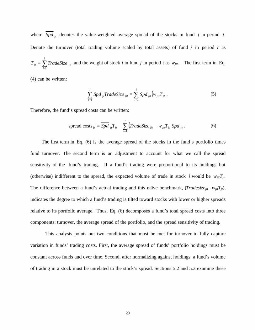
The first term in Eq. (6) is the average spread of the stocks in the fund’s portfolio times

fund turnover. The second term is an adjustment to account for what we call the spread

sensitivity of the fund’s trading. If a fund’s trading were proportional to its holdings but

(otherwise) indifferent to the spread, the expected volume of trade in stock i would be wjitTjt.

The difference between a fund’s actual trading and this naïve benchmark, (Tradesizejit -wjitTjt),

indicates the degree to which a fund’s trading is tilted toward stocks with lower or higher spreads

relative to its portfolio average. Thus, Eq. (6) decomposes a fund’s total spread costs into three

components: turnover, the average spread of the portfolio, and the spread sensitivity of trading.

This analysis points out two conditions that must be met for turnover to fully capture

variation in funds’ trading costs. First, the average spread of funds’ portfolio holdings must be

constant across funds and over time. Second, after normalizing against holdings, a fund’s volume

of trading in a stock must be unrelated to the stock’s spread. Sections 5.2 and 5.3 examine these

21

two conditions, respectively. Both sections conclude that the respective assumption is not valid.13

This explains the Table 4 findings that variation in turnover does a relatively poor job of

capturing variation in trading costs.

5.2. Turnover, average spreads, and trading costs

Figure 3 plots the distribution across funds in turnover, Tjt, and the average spread of fund

holdings ( )jtSpd . The figure is constructed by independently ranking funds into turnover

quintiles and spread quintiles, and then forming a five-by-five partition of the sample of funds

according to these quintile rankings. Panel A presents the number of funds in each cell of the

five-by-five partition. The area of each dot graphically represents the relative number of funds in

the corresponding cell. Panel B presents the average annual spread costs of the funds in each cell,

with the area of the dot graphically representing the relative magnitude of that cost. The average

turnover of the funds in each turnover quintile is listed in the row headings. Similarly, the

average spread of the funds’ holdings in each effective-spread quintile is listed in the column

heading.

There are several observations from Fig. 3. First, there is substantial variation in the

average spread of holdings across funds. Section 5.1 shows that turnover will be an accurate

proxy for trading costs only if trading costs are proportional to turnover (spread sensitivity close

to zero) and the proportionality coefficient (the fund’s average spread) is constant across funds.

Fig. 3 shows that one cannot apply a single proportionality coefficient in relating trading costs to

turnover without losing significant explanatory power. Both turnover and the average spread of

holdings are important determinants of funds’ spread costs. For example, the five funds in

turnover quintile 1 and spread quintile 5 have average annual spread costs of .46%, a magnitude

13 Chalmers and Kadlec (1998) use similar logic to argue that investors’ amortized spread costs are not fully captured by the

22

similar to that for the three funds in the opposite corner, turnover quintile 5 and spread quintile 1,

with annual spread costs averaging .57%. There are a number of similar examples in Panel B

which demonstrate that a fund’s annual spread costs depends on both the frequency of trade and

the average spread of the funds’ holdings.

Second, in Panel A, the number of funds along the diagonal, where turnover and average

spread of holdings are directly related, is surprising. For example, among funds that hold the

highest-spread stocks (average spread = 1.28%) the greatest concentration of funds occurs in the

highest turnover quintile (average turnover = 1.35). Recall that the quintile rankings are

independent, so funds in the high-turnover quintile have high turnover relative to all funds, not

just relative to other high-spread funds. One might expect that funds holding higher-spread

stocks would have relatively lower turnover rates, given that their turnover is particularly costly.

For example, Amihud and Mendelson (1986) discuss a clientele effect whereby investors with

short holding periods hold stocks with relatively low spreads and investors with long holding

periods hold stocks with relatively high spreads. A similar argument applies to the funds in the

lowest spread quintile. Most funds in this quintile are relatively inactive traders, despite the fact

that they hold relatively low spread stocks. These patterns are statistically significant: the p-value

for the null that there is no association between the row and column variable in Panel A, using a

chi-square test, is 0.015.

5.3 Spread sensitivity of trading

The spread sensitivity component of trading costs is negative if trading volume within the

fund is inversely related to the spread. We use a summary measure of spread sensitivity (the

second term in Eq. (6)) in decomposing trading costs. A more comprehensive measure of spread

spread and must consider turnover as well.

23

sensitivity is provided by regressing trading volume on spreads across portfolio holdings. This

section focuses on this measure. We have considered many specifications for this regression. All

have some disadvantage, econometric or otherwise. However, the conclusions regarding trading

behavior are robust across procedures and they collectively provide evidence that fund managers

are somewhat sensitive to costs imposed by the spread, after controlling for the fund’s holdings.

For brevity, we present only one of the many methods used to evaluate fund manager’s trading

sensitivity to spread costs.

For each fund, and each quarter, we estimate a regression where the dependent variable is

the volume of trade in various spread categories or bins, and the independent variables are the

total portfolio weight of stocks in the bin and the average spread of the stocks in the bin. Using

this approach, all stocks held or traded during the quarter are allocated into one of forty bins

according to their effective spread. The bins range from a spread of less than 0.20% to 4.0%,

with 0.10% increments. The total portfolio weight in each bin is determined, each quarter, as is

the total volume of transacting by the fund in each bin, each quarter. Thus, for each fund, and

each quarter we estimate a regression with 40 observations. Intuitively, the regressions test

whether the trading activity associated with a stock depends on the spread, after controlling for

the fund’s tendency to hold such stocks.

Table 6 reports average coefficient estimates from the above regressions. Perhaps not

surprisingly, there is a strong association between funds’ trading activity and their holdings. That

is, if a fund holds more of particular stock it tends to trade it more. The interesting result is the

incremental negative relation between trading activity and spread after controlling for holdings.

The t-statistic for this relation is –12, and in the various specifications attempted was never less

than –4. This indicates that on average, funds pay some attention to the spread in making trading

24

decisions. Thus, according to equation (6), this factor is likely to provide information about the

fund’s overall trading costs.

5.4 Fund returns and the components of trading costs

In results not tabulated we present a regression decomposition of funds’ annual spread

costs into the three components, turnover, average spread of holdings, and spread sensitivity.

The coefficient estimates are 0.005 (t=42), 0.100 (t=34) and 0.002 (t=4), respectively. This

suggests that all three components are important determinants of fund trading costs. In this

section we examine the relative contribution of the three components in explaining fund returns.

Table 7 reports time-series average coefficient estimates from regressions of fund returns

on expense ratios and the three components of spread costs. From Table 7, fund returns retain a

negative relation to expense ratios, though not as significantly as in the regressions of Table 5.

As in Carhart (1997), we find that fund returns are negatively related to fund turnover, although

the significance is generally marginal. The average coefficient estimate for turnover are –.02 (t-

statistic=-1.46), -.02 (t-statistic=-1.84), and -.03 (t-statistic=-2.60) for the regressions using raw

returns, CAPM-adjusted returns, and Carhart-adjusted returns, respectively.

We also find evidence that the other components of spread costs, average spread of

holdings, and spread sensitivity, help to explain fund returns. For example, the coefficient

estimate for average spread of holdings is negative in all three regressions and significant in the

regressions using raw returns and CAPM-adjusted returns. In particular, the average coefficient

estimate for average spread of holdings are –.96 (t-statistic=-1.76), -1.47 (t-statistic=-2.83), and -

0.12 (t-statistic=-0.55) for the regressions using raw returns, CAPM-adjusted returns, and

Carhart-adjusted returns, respectively. The coefficient estimate for spread sensitivity is also

negative in all three regressions, though it insignificant in each of the three regressions. From

25

this analysis we conclude that there is weak explanatory power to the non-turnover components

of trading costs.

6. Investment objectives and fund costs

Fund investment objective classifications are an important descriptor of mutual funds.

However, they are inherently subjective. Brown and Goetzman (1997) attack the subjective

nature of the classification system by examining the returns of mutual funds and classifying

them by their return characteristics, arguing that these are much more objective measures by

which funds can be categorized. Given the strong explanatory power for performance, it strikes

us that the expense ratios and trading costs that funds impose on investors provide useful

measures by which funds can be characterized. With this in mind, we provide evidence on the

question: to what extent is cross sectional variation in total fund costs, expense ratios and

trading costs, explained by existing investment-objective classifications?

Table 8 provides statistics on costs broken down by CRSP’s 1987 investment objectives

for our sample funds. In Panel A fund characteristics, most importantly the expense ratio and

trading costs, are presented. There is some variation in total costs across investment

objectives, particularly for maximum capital gains and growth categories. However, in

comparing this range of explained variation to Table 4 it is apparent that existing objective

classifications have little association with costs and that most of the cross sectional variation in

costs occurs within objectives instead of across objectives. To highlight this point, the 25th –

75th percentile ranges for total fund costs (not reported in Table 8) are 159 bp to 254 bp for

Maximum capital gain, 149 bp to 231 bp for Growth funds, and 105 to 178 for Growth and

Income funds. The large variation within investment objective supports the notion that

26

classification based upon trading costs provides valuable information beyond that provided by

the investment objective.

Table 8 Panel B summarizes the characteristics of the stocks held by investment

objective. The investment objectives do appear to correspond with stock characteristics in the

manner that one might expect. For example, average effective spreads are .59% maximum

capital gain and .49% for growth funds while the stocks that Growth and Income funds own

have average effective spreads of .35%. In addition, the other stock characteristic variables

conform to the observation that more risky stock attributes are associated with maximum

capital gain and growth objectives. Even so, the riskiest objective holds very large stocks, size

rank of 8.6, with low effective spreads (rank=2.8), below median standard deviations (rank =

4.3), and above median dividend yields (rank=6.1).

7. Conclusions

We estimate the annual costs of fund managers’ trades and find these costs to have a

substantial negative association with return performance. There are many interesting contexts

in which to interpret the evidence in our paper. Grossman and Stiglitz (1980) suggest that an

informed trader will not trade in stocks where the expected value of the information is less than

the costs of executing the trade. One interpretation of our evidence is that mutual fund

managers do not follow this rule. Alternatively, it could be that much of the trading costs we

observe are related to the provision of liquidity as discussed in Edelen (1999). To the extent

that this trading is unavoidable, the negative association between fund returns and trading costs

suggests that it pays to have fund managers who mitigate the cost of such trades. Finally, a

plausible, although unlikely interpretation for our results is that poor returns cause higher

27

trading costs because investors leave funds with poor returns which generates additional

trading costs. We find this unlikely because inflows also create liquidity costs and Sirri and

Tufano (1998) and Del Guercio and Tkac (1999) find that inflow tends to follow good

performance, while fund outflows are relatively insensitive to fund returns.

A practical issue that arises from our analysis is that it is costly to obtain direct estimates

of funds’ trading costs. Given their importance in explaining fund returns, a low cost proxy for

trading costs may be valuable. Our evidence suggests that a truly discriminating proxy needs

to go beyond turnover. Unfortunately, the other two components of trading costs, the

weighted-average spread and cost sensitivity of trading, are not readily observable. Thus, the

search for a low-cost proxy for these components would have significant practical value.

28

References

Amihud, Y., Mendelson, H., 1986. Asset pricing and the bid-ask spread. Journal of FinancialEconomics 17, 223-249.

Bogle, John C., Bogle on Mutual Funds: New Perspectives for the Intelligent Investor, IrwinProfessional Publishing, 1994, Burr Ridge, IL.

Brown, S.J., W. N. Goetzmann, 1997. Mutual Fund Styles. Journal of Financial Economics, 43,373-399.

Carhart, M, 1997, On persistence in mutual fund performance, The Journal of Finance, 52, 1, 57-82.

Chalmers, J.M.R., Kadlec, G.B., 1998. An empirical examination of the amortized spread. TheJournal of Financial Economics, 48, 2, 159-188.

Chan, L.K.C. and J. Lakonishok, 1993. Institutional trades and intraday stock price behavior,Journal of Financial Economics, 33. 173-199.

Chan, L.K.C., J. Lakonishok, 1995. The behavior of stock prices around institutional trades,Journal of Finance, 50, 1147-1174.

Chan, L.K.C., J. Lakonishok, 1997. Institutional equity trading costs: NYSE versus Nasdaq,Journal of Finance. 52, 713-735.

Collins, S. and P. Mack, 1997, The optimal amount of assets under management in the mutualfund industry, Financial Analysts Journal, September/October, 67-73.

Daniel, K., M. Grinblatt, S. Titman, and R. Wermers, 1997, Measuring mutual fund performancewith characteristic-based benchmarks, The Journal of Finance, 52, 1035-1058.

Del Guercio, D., 1996, The distorting effect of the prudent-man laws on institutional equityinvestments, Journal of Financial Economics, 40, 1, 31-62.

Del Guercio, D. and P.A. Tkac, 1999, The determinants of the flow of funds of managedportfolios: Mutual funds versus pension funds, working paper University of Oregon.

Edelen, R., 1999. Investor flows and the assessed performance of open-end mutual funds,Journal of Financial Economic, 53, 439-466.

Elton, E.J., M.J. Gruber, S. Das, and M. Hlavka, 1993, Efficiency with costly information: areinterpretation of evidence from managed portfolios, Review of Financial Studies, 6,1, 1-22.

29

Falkenstein, E. G., 1996, Preferences for stock characteristics as revealed by mutual fundportfolio holdings, Journal of Finance, 51, 1, 111-135.

Fama, E.F., K.R. French, 1993. Common risk factors in the returns on bonds and stocks, Journal offinancial economics 33, 3-53.

Fama, E.F. and J. MacBeth, 1973, Risk, return, and equilibrium: Empirical tests, Journal of PoliticalEconomy 81, 607-636.

Gompers, P. and A. Metrick, 1998, How are large institutions different from other investors?Why do these differences matter for Equity Prices and Returns? Working paper HarvardUniversity and National Bureau of Economic Research.

Grinblatt, M. and S. Titman, 1989, Mutual fund performance: An analysis of quarterly holdings,Journal of Business 62, 393-416.

Grossman, S., and J. Stiglitz, 1980, On the impossibility of informational efficient markets,American Economic Review, 70, 393-408.

Gruber, M. J., 1996, Another Puzzle: The Growth in Actively Managed Mutual Funds, The Journalof Finance, 51, 783-810.

Huddart, S. and V.G. Narayaran, (1997). Inventory rules, taxation and institutions’ tradingdecisions. Working paper, Duke University.

Jensen, M.C., 1968, The performance of mutual funds in the period 1945-1964, Journal ofFinance, 23, 389-416.

Jones, C. and M. Lipson, 1999, Execution costs of institutional equity orders, Journal ofFinancial Intermediation, 8,123-140.

Keim, D.B. and A. Madhavan, 1995. Anatomy of the trading process, Empirical evidence on thebehavior of institutional traders, Journal of Financial Economics. 37, 371-398.

Keim, D.B. and A. Madhavan, 1997. Transactions costs and investment style: an inter-exchangeanalysis of institutional equity trades, Journal of Financial Economics, 46, 265-292.

Malkiel, B.G., 1995, Returns from investing in equity mutual funds 1971 to 1991, Journal ofFinance, 50, 549-572.

Sirri, E.R. and P. Tufano, 1998, Costly search and mutual fund flows, Journal of Finance, 53,1589-1622.

Tufano, P. and M. Sevick, 1997, Board structure and fee-setting in the U.S. mutual fund industry46, 321-355.

30

Wermers, R., 1999, Mutual fund herding and the impact on stock prices, Journal of Finance, 54,2, 581-622.

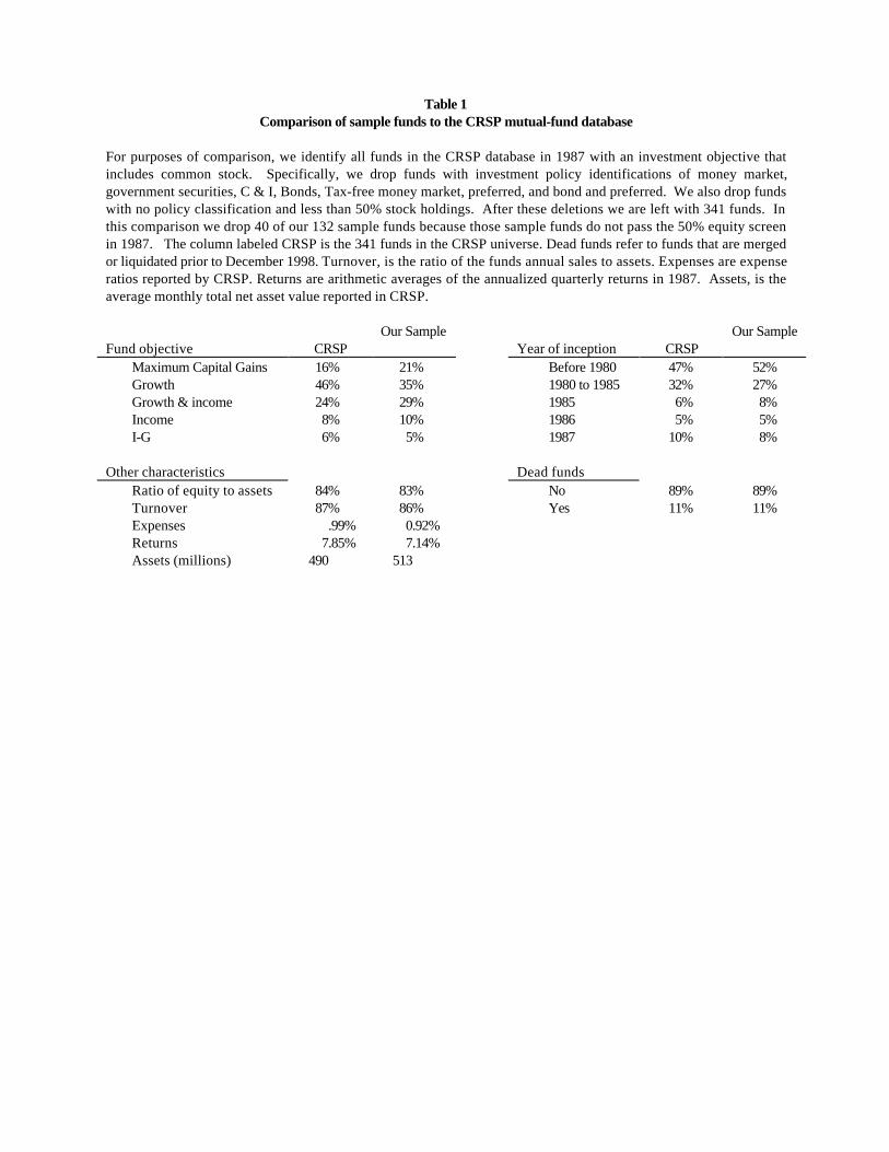
Table 1Comparison of sample funds to the CRSP mutual-fund database

For purposes of comparison, we identify all funds in the CRSP database in 1987 with an investment objective thatincludes common stock. Specifically, we drop funds with investment policy identifications of money market,government securities, C & I, Bonds, Tax-free money market, preferred, and bond and preferred. We also drop fundswith no policy classification and less than 50% stock holdings. After these deletions we are left with 341 funds. Inthis comparison we drop 40 of our 132 sample funds because those sample funds do not pass the 50% equity screenin 1987. The column labeled CRSP is the 341 funds in the CRSP universe. Dead funds refer to funds that are mergedor liquidated prior to December 1998. Turnover, is the ratio of the funds annual sales to assets. Expenses are expenseratios reported by CRSP. Returns are arithmetic averages of the annualized quarterly returns in 1987. Assets, is theaverage monthly total net asset value reported in CRSP.

Fund objective CRSPOur Sample

Year of inception CRSPOur Sample

Maximum Capital Gains 16% 21% Before 1980 47% 52%Growth 46% 35% 1980 to 1985 32% 27%Growth & income 24% 29% 1985 6% 8%Income 8% 10% 1986 5% 5%I-G 6% 5% 1987 10% 8%

Other characteristics Dead fundsRatio of equity to assets 84% 83% No 89% 89%Turnover 87% 86% Yes 11% 11%Expenses .99% 0.92%Returns 7.85% 7.14%Assets (millions) 490 513

Table 2Characteristics of sample funds and their holdings

Panel A: Sample fundsFund assets represent total assets under management, as reported by CDA (quarterly observations). Equity / FundAssets is the average equity value held by the fund divided by fund value reported by CDA. Fund returns areannualized monthly data from CRSP. Turnover is annual fund sales divided by fund assets. Inflow and outflow arethe annual cash flows into and out of the mutual funds scaled by fund assets.

N=132 Funds. Mean 10% 25% Median 75% 90%Fund assets (millions) 374 35 68 153 468 1,085Equity / Fund Assets .81 .62 .73 .85 .90 .94Fund returns (%) 13.2 3.9 10.0 13.9 16.8 22.4Turnover .76 .27 .45 .70 .99 1.45Inflow (N = 126 Funds) .39 .09 .16 .25 .48 .76Outflow (N =126 Funds) .40 .14 .19 .27 .42 .69

Panel B: Stocks held by sample fundsNumber of stocks is the average number of stocks held in the fund portfolio each quarter. Standard deviation is theannualized monthly standard deviation of return. Effective spread is the transaction-size-weighted average effectivespread of each stock over the quarters in which the stock is held. Prior year return is the raw return of the stock inthe year prior to the observation. All rank variables are relative to an equal-weighted decile ranking of the universe ofstocks available on CRSP (NYSE/AMEX/NASDAQ) (1 low, 10 high).

N=132 Funds Mean 10% 25% Median 75% 90%Number of Stocks 82 39 55 73 98 132

Market Value Equity (millions) 4,662 547 2,514 4,804 7,608 8,674Rank 9.2 7.0 7.9 8.5 8.8 8.9

Price 39 23 33 40 46 51Rank 8.7 7.6 8.3 8.9 9.3 9.6

Standard Deviation of return .36 .27 .30 .34 .39 .47Rank 3.6 2.2 2.7 3.3 4.2 5.3

Dividend Yield 3.0% 1.0% 1.9% 3.0% 4.0% 4.6%Rank 7.0 5.0 6.0 7.3 8.0 8.7

Effective Spread .46% .29% .33% .40% .50% .62%Rank 2.11 1.3 1.5 1.8 2.4 3.2

Beta 1.03 .80 .90 1.01 1.15 1.28Rank 5.35 4.2 4.8 5.3 6.0 6.6

Prior year return .20 .10 .14 .18 .26 .35Rank 6.8 6.1 6.4 6.7 7.1 7.5

Book-to-market .62 .45 .51 .62 .72 .78Rank 5.1 4.0 4.5 5.2 5.8 6.3

Table 3Fund expenses, trading costs and capital gains

All data expressed as annual percent of fund assets. Expense ratio is annual expenses scaled by fund assets asreported by CRSP and does not include sales charges (loads) or brokerage commissions. Spread costs are effectivespreads times dollar trade size summed over all trades in a given year, for a given fund, scaled by fund assets.Brokerage commissions are observed semi-annually and reported on an annualized basis. We estimate data onbrokerage commissions for 33 of 132 funds. Total fund costs is the sum of the expense ratio, spread costs, andbrokerage commissions. Realized gains measures the annualized capital gains realized during the period. Total gain isthe hypothetical capital gain if all positions were liquidated. Correlations are calculated by first averaging over timeeach fund’s data, then computing the correlation across funds.

Data (% of fund assets) Mean 10% 25% Median 75% 90%Expense ratio 1.07 .66 .80 1.03 1.28 1.49Spread costs .47 .15 .25 .39 .62 .88Brokerage commissions .31 .10 .18 .28 .42 .54Spread + Brokerage .78 .30 .44 .70 1.03 1.37Total Fund Expenditures 1.85 1.01 1.35 1.74 2.28 2.76Realized gains 5.32 .09 2.58 4.95 8.01 12.07Total gain 9.57 .45 5.49 9.77 14.26 19.38

CorrelationExpense ratio Spread costs

Brokerage commissions .52 .53Spread costs .37Spread + commissions .52

Table 4Average fund returns by cost quintiles

All data expressed in annual terms. Funds are assigned to quintiles each quarter on the basis of total cost, trading costs, expense ratios and turnover (1=low). Thetable presents the average value of the indicated variable within quintile sub-samples. Total cost is the sum of expense ratios, spread costs, and brokeragecommissions. Spread costs are effective spreads times dollar trade size summed over all trades in a given year, for a given fund, scaled by total equity. Carhartadjusted returns are raw fund returns minus the predicted return from the four-factor model presented in Carhart (1997). CAPM adjusted returns are raw fund returnsminus the expected return from the CAPM. T-statistics are reported which test the hypothesis that the mean quintile 1 value minus the mean quintile 5 value is zero.The turnover quintiles exclude 4.6% of the observations because of missing CRSP turnover. Below the panels the mean value across all observations is reported forthe sum of the adjusted return measures and total fund costs. The t-statistic for this value tests the null that the sum is zero. ** p-value < .05, * p-value < .10.

Total Fund Cost Quintile t-statistic Trading Cost Quintile t-statistic1 2 3 4 5 (Q1-Q5) 1 2 3 4 5 (Q1-Q5)

Expense Ratio 0.65% 0.86% 1.03% 1.15% 1.40% -60.00** 0.76% 0.95% 1.04% 1.11% 1.24% -36.73**Spread Cost 0.16% 0.33% 0.45% 0.66% 1.18% -63.51** 0.13% 0.29% 0.45% 0.67% 1.23% -72.93**Brokerage commissions 0.09% 0.17% 0.26% 0.37% 0.55% -64.34** 0.08% 0.16% 0.25% 0.38% 0.56% -68.73**Total Costs 0.90% 1.36% 1.74% 2.18% 3.12% -112.94** 0.97% 1.40% 1.74% 2.16% 3.03% -94.71**

Carhart Adjusted Returns -0.77% -0.87% -1.04% -1.73% -4.38% 4.34** -0.25% -0.94% -0.87% -3.09% -3.62% 4.06**CAPM Adjusted Returns -0.41% -1.75% -1.52% -2.32% -6.26% 6.24** 0.06% -1.68% -1.68% -3.68% -5.25% 5.64**Returns 14.52% 13.42% 13.93% 12.66% 9.76% 1.95* 14.14% 13.89% 14.06% 11.88% 10.31% 1.60

Expense Ratio quintiles t-statistic Turnover Quintiles t-statistic1 2 3 4 5 (Q1-Q5) 1 2 3 4 5 (Q1-Q5)

Expense Ratio 0.59% 0.81% 0.99% 1.15% 1.55% -91.18** 0.81% 0.91% 1.01% 1.15% 1.18% -27.71**Spread Cost 0.35% 0.42% 0.52% 0.73% 0.76% -24.02** 0.24% 0.38% 0.53% 0.66% 0.96% -47.34**Brokerage commissions 0.16% 0.22% 0.28% 0.33% 0.44% -32.36** 0.11% 0.17% 0.28% 0.35% 0.51% -53.59**Total Costs 1.10% 1.45% 1.79% 2.21% 2.74% -64.75** 1.16% 1.47% 1.82% 2.15% 2.65% -58.59**

Carhart Adjusted Returns -1.31% -1.70% -1.06% -1.11% -3.63% 2.79** -1.10% -1.32% -1.51% -1.88% -2.52% 1.59CAPM Adjusted Returns -1.01% -1.95% -1.57% -2.75% -4.98% 4.20** -3.28% -2.05% -2.13% -2.30% -2.82% -.45Returns 14.50% 13.04% 12.67% 13.12% 10.97% 1.44 11.87% 13.23% 13.67% 13.46% 12.18% -.13

Mean Carhart adjusted return + total fund costs = .11%, t-statistic=.43Mean CAPM adjusted return + total fund costs = -.59%, t-statistic=-2.12*

Table 5Expenses, spread costs and fund returns

Coefficients reported below are time-series averages of coefficients from 64 cross-sectional regressions of monthlyfund returns on expenses and spread costs following Fama-MacBeth (1973). Raw fund returns are unadjusted fundreturns. The returns are measured net of fund expenses, fees, and transaction costs (excluding load fees). CAPM-adjusted returns are raw fund returns minus the expected return as specified by the CAPM. Carhart-adjusted returnsare raw fund returns minus the expected return as specified by a four factor model used in Carhart (1997). Expensesare the funds expense ratio from CRSP. Spread costs are the expenditures we estimate the fund has made on bid-askspread related costs scaled by equity value. * indicates p-value < 10% and ** indicates the p-value < 5%.

Independentvariables

Raw FundReturns

CAPM-adjustedReturns

Carhart-adjustedReturn

Intercept .01** .002** .002**(2.5) (2.93) (2.22)

Expenses -1.72* -2.22** -1.77**(-1.74) (-2.72) (-2.90)

Spread Expenditures -3.43* -5.21** -3.22**(-1.98) (-3.20) (-2.95)

N (cross-sections) 64 64 64

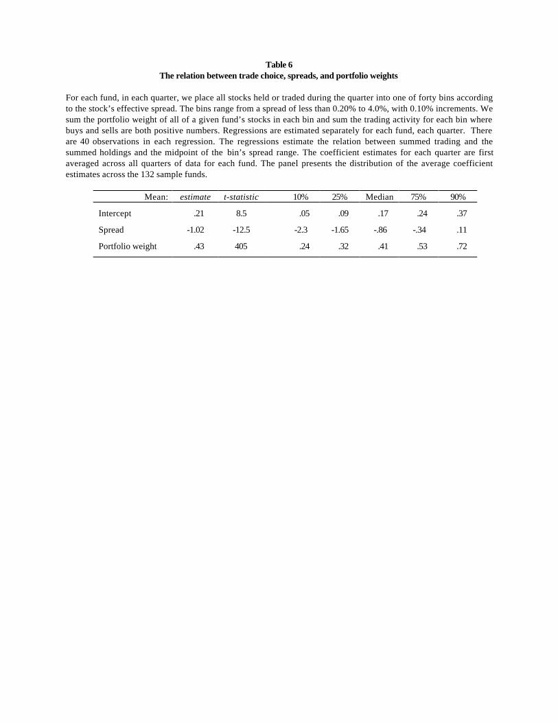
Table 6 The relation between trade choice, spreads, and portfolio weights

For each fund, in each quarter, we place all stocks held or traded during the quarter into one of forty bins accordingto the stock’s effective spread. The bins range from a spread of less than 0.20% to 4.0%, with 0.10% increments. Wesum the portfolio weight of all of a given fund’s stocks in each bin and sum the trading activity for each bin wherebuys and sells are both positive numbers. Regressions are estimated separately for each fund, each quarter. Thereare 40 observations in each regression. The regressions estimate the relation between summed trading and thesummed holdings and the midpoint of the bin’s spread range. The coefficient estimates for each quarter are firstaveraged across all quarters of data for each fund. The panel presents the distribution of the average coefficientestimates across the 132 sample funds.

Mean: estimate t-statistic 10% 25% Median 75% 90%

Intercept .21 8.5 .05 .09 .17 .24 .37

Spread -1.02 -12.5 -2.3 -1.65 -.86 -.34 .11

Portfolio weight .43 405 .24 .32 .41 .53 .72

Table 7Fund returns and the components of spread costs

Coefficients reported below are time-series averages of coefficients from 64 cross-sectional Fama-MacBeth (1973)regressions of monthly fund returns on expenses, turnover, average effective spread of holdings, and the spreadsensitivity. Raw fund returns are unadjusted fund returns. Fund returns are measured net of fund expenses, fees,and transaction costs, excluding load fees. CAPM-adjusted returns are raw fund returns minus the expected returnas specified by the CAPM. Carhart-adjusted returns are raw fund returns minus the expected return as specified by afour factor model used in Carhart (1997). Expenses are the funds expense ratio from CRSP. Fund turnover is estimatedfrom the CDA data and is measured as the average of purchases plus sales divided by fund assets. Average spreadis the value-weighted average effective spread of the fund’s stock holdings. Spread sensitivity is defined in eq. (6)and measures the tendency of the fund manager to trade stocks that are more or less costly to trade than the averagestock that the fund holds. * indicates p-value < 10% and ** indicates the p-value < 5%.

Independentvariables

Raw FundReturns

CAPM-adjustedReturns

Carhart-adjustedReturn

Intercept .02** .005** .002**(2.99) (2.81) (2.01)

Expenses -.81 -1.17 -1.81**(-.97) (-1.60) (-2.79)

Fund Turnover -1.90 -.02* -.03**(-1.46) (-1.84) (-2.60)

Average Spread -.96* -1.47** -.12(-1.76) (-2.83) (-.55)

Spread Sensitivity -.05 -.07 -.03(-.87) (-1.33) (-.61)

N (cross-sections) 64 64 64

Table 8Characteristics of funds and their holdings by investment objective

Using the CRSP fund objective codes from 1987 we characterize the average values of funds broken down byinvestment objective. Ranks are computed annually relative to the universe of available data in each year. Theinvestment objective we call aggressive growth is classified by CRSP as maximum captital gains and I-G appears to besynonymous with an investment style of balanced.

Panel A: Fund characteristics by investment objectiveFund characteristics Aggressive

GrowthGrowth Growth &

IncomeIncome I-G

Number of funds 32 48 33 11 8Fund Assets (millions) 365 281 527 427 265Fund Return 14.1% 13.4% 13.9% 8.4% 12.6%Expense ratio 1.15% 1.13% 0.95% 0.98% 0.96%Spread Cost 0.65% 0.51% 0.35% 0.34% 0.16%Brokerage Commission 0.35% 0.35% 0.26% 0.29% 0.14%Total Fund Costs 2.15% 1.99% 1.56% 1.61% 1.39%Realized Capital Gains 2.73% 6.61% 6.76% 4.56% 2.97%Total Gains 6.81% 11.75% 11.89% 2.21% 8.04%Turnover .94 .77 .63 .88 .65Ratio of Equity to Assets .83 .83 .83 .83 .56Fund Inflows .46 .48 .25 .35 .25Fund Outflows .47 .51 .25 .26 .25

Panel B: Stock holdings’ characteristics by investment objectiveAll rank variables are relative to an equal-weighted decile ranking of the universe of stocks available on CRSP(NYSE/AMEX/NASDAQ) with 1 low and 10 high. Number of stocks is the average number of stocks held in the fundportfolio each quarter. Standard deviation is the annualized monthly standard deviation of return. Effective spread isthe average effective spread for the stocks held by each fund. The effective spread for each stock is a transaction-size-weighted average effective spread over the quarter in which the stock is held by any fund. Prior year return isthe raw return of the stock in the year prior to the observation.Stock Holdings’ Aggressive

GrowthGrowth Growth&

IncomeIncome I-G

Number of stocks held 94 89 71 81 47

Market Value Equity (mil) 2,781 3,715 6,396 6,181 8,636Rank 8.6 9.1 9.6 9.6 9.8

Price 36.27 35.84 44.60 41.08 47.03Rank 8.0 8.5 9.2 9.0 9.4

Standard Deviation of Return .40 .38 .31 .31 .27Rank 4.3 4.0 2.9 2.8 2.3

Dividend yield 2.06% 2.62% 3.62% 4.44% 4.16%Rank 6.1 6.5 7.9 8.4 8.5

Effective spread .59% 0.49% 0.35% .37% .30%Rank 2.8 2.3 1.6 1.7 1.4

Prior year return .22 .23 .19 .15 .15Rank 6.6 6.8 6.8 6.5 6.9

Book-to-Market .59 .57 .66 .74 .67Rank 4.9 4.9 5.4 5.9 5.5

Beta 1.1 1.1 .9 .9 .8Rank 5.9 5.7 4.8 4.7 4.3

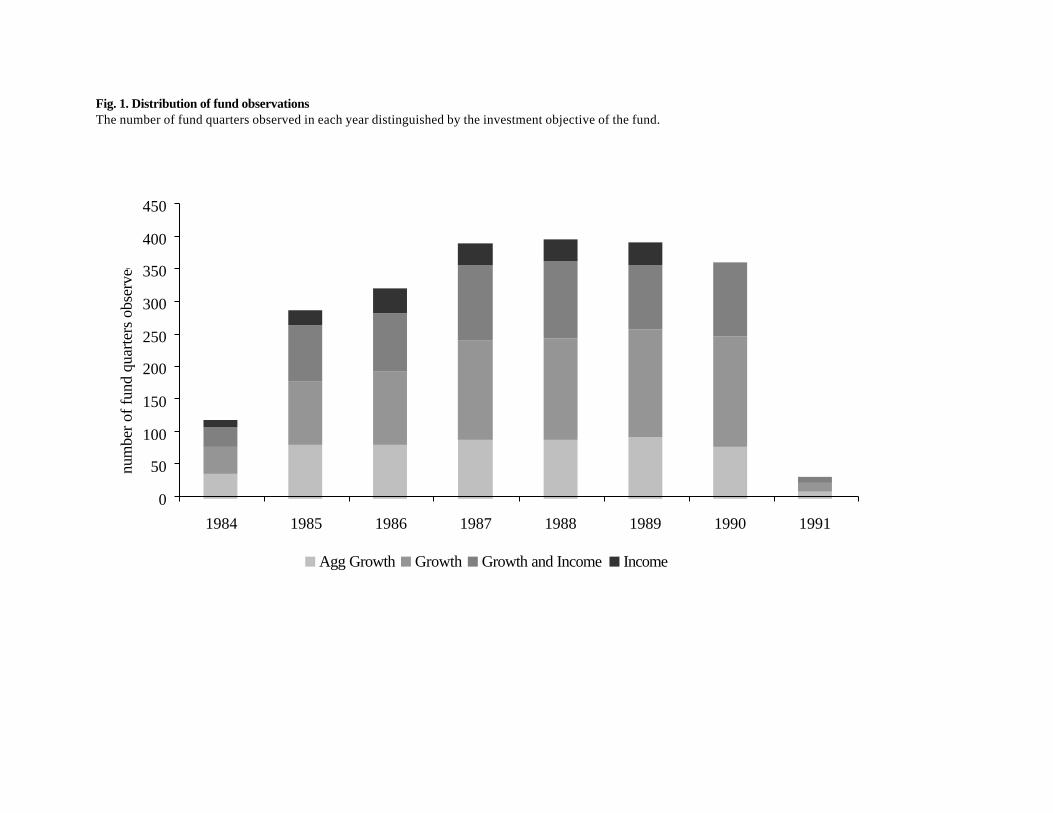
Fig. 1. Distribution of fund observationsThe number of fund quarters observed in each year distinguished by the investment objective of the fund.

0

50

100

150

200

250

300

350

400

450

1984 1985 1986 1987 1988 1989 1990 1991

num

ber o

f fun

d qu

arte

rs o

bser

ved

Agg Growth Growth Growth and Income Income

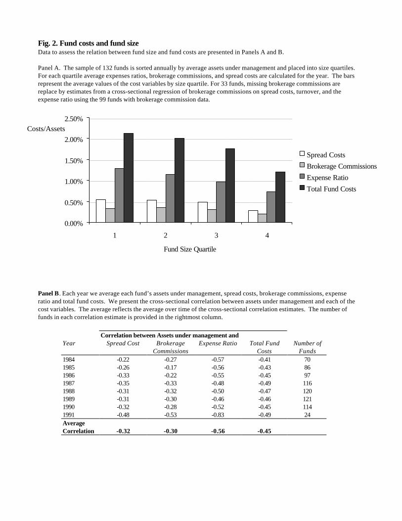
Fig. 2. Fund costs and fund sizeData to assess the relation between fund size and fund costs are presented in Panels A and B.

Panel A. The sample of 132 funds is sorted annually by average assets under management and placed into size quartiles.For each quartile average expenses ratios, brokerage commissions, and spread costs are calculated for the year. The barsrepresent the average values of the cost variables by size quartile. For 33 funds, missing brokerage commissions arereplace by estimates from a cross-sectional regression of brokerage commissions on spread costs, turnover, and theexpense ratio using the 99 funds with brokerage commission data.

Panel B. Each year we average each fund’s assets under management, spread costs, brokerage commissions, expenseratio and total fund costs. We present the cross-sectional correlation between assets under management and each of thecost variables. The average reflects the average over time of the cross-sectional correlation estimates. The number offunds in each correlation estimate is provided in the rightmost column.

Correlation between Assets under management andYear Spread Cost Brokerage

CommissionsExpense Ratio Total Fund

CostsNumber of

Funds1984 -0.22 -0.27 -0.57 -0.41 701985 -0.26 -0.17 -0.56 -0.43 861986 -0.33 -0.22 -0.55 -0.45 971987 -0.35 -0.33 -0.48 -0.49 1161988 -0.31 -0.32 -0.50 -0.47 1201989 -0.31 -0.30 -0.46 -0.46 1211990 -0.32 -0.28 -0.52 -0.45 1141991 -0.48 -0.53 -0.83 -0.49 24AverageCorrelation -0.32 -0.30 -0.56 -0.45

0.00%

0.50%

1.00%

1.50%

2.00%

2.50%

1 2 3 4

Fund Size Quartile

Costs/Assets

Spread Costs

Brokerage Commissions

Expense Ratio

Total Fund Costs

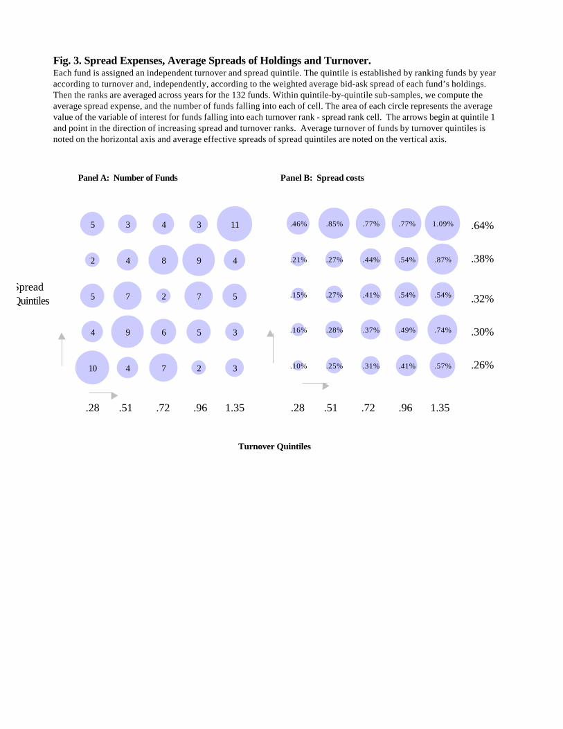
Fig. 3. Spread Expenses, Average Spreads of Holdings and Turnover.Each fund is assigned an independent turnover and spread quintile. The quintile is established by ranking funds by yearaccording to turnover and, independently, according to the weighted average bid-ask spread of each fund’s holdings.Then the ranks are averaged across years for the 132 funds. Within quintile-by-quintile sub-samples, we compute theaverage spread expense, and the number of funds falling into each of cell. The area of each circle represents the averagevalue of the variable of interest for funds falling into each turnover rank - spread rank cell. The arrows begin at quintile 1and point in the direction of increasing spread and turnover ranks. Average turnover of funds by turnover quintiles isnoted on the horizontal axis and average effective spreads of spread quintiles are noted on the vertical axis.

Panel A: Number of Funds Panel B: Spread costs

Turnover Quintiles

SpreadQuintiles

27410

35694

57275

4984

11343

2

3

5 .46%

.57%

.21%

.85% .77% .77% 1.09%

.27% .44% .54% .87%

.15% .27% .41% .54% .54%

.16% .28% .37% .49% .74%

.10% .25% .31% .41%

.64%

.38%

.32%

.30%

.26%

.28 .51 .72 .96 1.35 .28 .51 .72 .96 1.35