an analysis on the correlation between atmospheric
TRANSCRIPT
South Dakota State University South Dakota State University
Open PRAIRIE: Open Public Research Access Institutional Open PRAIRIE: Open Public Research Access Institutional
Repository and Information Exchange Repository and Information Exchange
Electrical Engineering and Computer Science Plan B Projects
Department of Electrical Engineering and Computer Science
2019
An Analysis on the Correlation Between Atmospheric Parameters An Analysis on the Correlation Between Atmospheric Parameters
and TOA Reflectance of Pseudo Invariant Calibration Sites (PICS) and TOA Reflectance of Pseudo Invariant Calibration Sites (PICS)
Yugeen Chaulagain South Dakota State University, [email protected]
Follow this and additional works at: https://openprairie.sdstate.edu/ee-cs_planb
Part of the Electrical and Computer Engineering Commons, Remote Sensing Commons, and the
Spatial Science Commons
Recommended Citation Recommended Citation Chaulagain, Yugeen, "An Analysis on the Correlation Between Atmospheric Parameters and TOA Reflectance of Pseudo Invariant Calibration Sites (PICS)" (2019). Electrical Engineering and Computer Science Plan B Projects. 1. https://openprairie.sdstate.edu/ee-cs_planb/1
This Plan B - Open Access is brought to you for free and open access by the Department of Electrical Engineering and Computer Science at Open PRAIRIE: Open Public Research Access Institutional Repository and Information Exchange. It has been accepted for inclusion in Electrical Engineering and Computer Science Plan B Projects by an authorized administrator of Open PRAIRIE: Open Public Research Access Institutional Repository and Information Exchange. For more information, please contact [email protected].
An Analysis on the Correlation Between Atmospheric Parameters and TOA Reflectance of
Pseudo Invariant Calibration Sites (PICS)
By
Yugeen Chaulagain
A research paper submitted in the partial fulfilment of the requirement for the
Master of Science
Major in Electrical Engineering
South Dakota State University
2019
TABLE OF CONTENTS
CHAPTER 1 Introduction………………………………………………………….….………1
1.1. Significance of calibration………………………………………………………..............1
1.2. Objective………………………………………………………………………………….2
1.3. Definitions of Atmospheric Parameters Considered in the Paper…………………….….2
1.3.1. Relative Humidity…………………………………………………………………3
1.3.2. Atmospheric Pressure (Barometric Pressure) …………………………………….3
1.4. Relative Spectral Response of Landsat-7 ETM+ and Landsat-8 OLI……………………4
CHAPTER 2 METHODOLOGY………………………………………………………….….6
2.1 Site Selection………………………………………………………………………….….6
2.1.1 Algodones Dunes………………………………………………………….…….….7
2.1.2 Wadi ad-Dawasir, Saudi Arabia……………………………………………………8
2.2 Analysis Methodology……………………………………………………………………8
2.2.1 Image Processing and Pre-processing……………………………………………...8
2.2.2 Deriving the Relationships Between TOA Reflectance and Atmospheric
Parameter…………………………………………………………………….…………...9
2.2.3 Consideration of Higher-Order and/or Nonlinear Atmospheric Parameter
Model……………………………………………………………………………………10
2.2.4 BRDF Normalization……………………………………………………………...11
CHAPTER 3 Result………………………………………………………………………….12
3.1. Algodones Dunes…………………………………………………………………….….12
3.1.1. Relationship Between TOA Reflectance and Absolute Humidity—Landsat 7
ETM+………………………………………………………………………………12

3.1.2. Relationship Between TOA Reflectance and Atmospheric Pressure—Landsat 7
ETM+………………………………………………………………………………17
3.1.3. Relationship Between TOA Reflectance and Absolute Humidity—Landsat 8
OLI…………………………………………………………………………………19
3.1.4. 3.1.1 Relationship Between TOA Reflectance and Atmospheric Pressure—
Landsat 8 OLI………………………………………………………………………21
3.2. Wadi ad-Dawasir Desert Site……………………………………………………………27
3.2.1. Relationship Between TOA Reflectance and Absolute Humidity……………….27
3.2.2. Relationship Between TOA Reflectance and Atmospheric Pressure……………29
3.3. Effects of BRDF Normalization………………………………………………………...34
CHAPTER 4 Conclusion and Future Direction……………………………………………...37
4.1. Processing Recommendations……………………………………………….………….38
4.2. Future Directions…………………………………………….………………………….39
CHAPTER 5 References…………………………………….….……………………………40
1
CHAPTER 1
INTRODUCTION
1.1 Significance of Calibration
The sensors onboard the Landsat series satellites have recorded numerous images of the Earth’s
surface since the beginning of the Landsat program in 1972. Each generation of sensor has been
built with increased spectral, spatial, and radiometric resolution, leading to increased use of their
imagery to study natural and human-induced changes to the planet. To ensure reliable information
is derived from the image data, the sensors need to be accurately calibrated, both radiometrically
and geometrically.
Radiometric calibration of satellite-based imaging sensors has been extensively studied, and can
be absolute or relative in nature. Absolute radiometric calibration of an individual sensor provides
gains and offsets used to convert raw image pixel values to accurate estimates of top-of-atmosphere
(TOA) radiance and/or reflectance. Relative radiometric calibration determines factors applied to
each detector’s raw pixel values to equalize the detector’s radiometric response.
The information required to perform radiometric calibration can be acquired from measurements
obtained with sources onboard the sensor (e.g. solar diffuser panels, lamps, thermal blackbody
sources, etc.), or from measurements derived directly from image data. Pseudo Invariant
Calibration Sites (PICS), primarily located in desert or other arid regions, have demonstrated
excellent potential as sources for image data used in radiometric calibration. They offer consistent
temporal, spatial, and spectral stability to within 3% [1]. If PICS-based calibration results are
compared with onboard calibration results, it can help to confirm whether any observed changes
in radiometric response are due to changes to the sensor itself.
2
Several works were developed using PICS for trending of sensors gains, sensors cross-calibration,
and, more recently, absolute calibration [2]. However, one issue that has not yet been addressed
and studied thoroughly was the effects of the atmosphere on PICS. Water vapor, barometric
pressure, ozone, and aerosols present in the atmosphere alter the amount of solar energy striking
the Earth’s surface through scattering and absorption processes that are wavelength dependent. For
PICS, it has been estimated that up to a third of the total estimated uncertainty is due to uncorrected
atmospheric effects [2]. As PICS are located in drier regions, the effects of atmospheric water
vapor are generally minimized. However, the lower the temporal uncertainty of the site, the more
important it is to understand its atmosphere.
1.2 Objective
The objective of this work is to understand and quantify the relationship(s) between atmospheric
parameters and TOA reflectance. The analysis uses Landsat-7 ETM+ and Landsat-8 OLI images
data acquired over the Algodones Dunes and a desert site near Wadi ad-Dawasir, Saudi Arabia.
The analysis focuses on atmospheric water content and barometric pressure, as ground truth
measurements of these quantities are likely to be readily available from relatively nearby weather
stations. Section II of the paper discusses the methodology used in the analysis. Section III presents
the analysis results. Finally, Section IV provides a summary and considers potential directions for
future investigation.
1.3 Definition of Atmospheric Parameters Considered in the Paper
This section briefly defines the atmospheric parameters considered in this work: relative (and
absolute) humidity, and atmospheric pressure. These parameters were chosen because they were
the most readily available in the weather station data. Humidity was the selected parameter for
characterization of the longer wavelength bands,
3
1.3.1 Relative Humidity
Relative humidity is defined as the ratio percentage of the water vapor pressure to the saturation
water vapor pressure at the gas temperature (273° K) [3]:
𝑅𝑅𝑅𝑅 = 𝑃𝑃𝑤𝑤𝑃𝑃𝑊𝑊𝑊𝑊
× 100% (1)
where pw and pws are the absolute water vapor pressure and saturation water vapor pressure in Pa,
respectively. The saturation water vapor pressure is the maximum pressure possible by water vapor
at a given temperature.
Relative humidity is a function of the ambient air temperature through pws:
𝑝𝑝𝑤𝑤𝑤𝑤 = 1𝑇𝑇8.2 × exp (77.345 + 0.0057 × 𝑇𝑇 − 7235
𝑇𝑇) (2)
The absolute humidity is defined as the mass of water vapor in a given volume. It is also a function
of the ambient air temperature.
𝐴𝐴𝑅𝑅 = 𝑐𝑐 × 𝑝𝑝𝑤𝑤𝑇𝑇
(3)
where c = 2.16679 gK/J and T is the ambient air temperature in °K.
Relative humidity can be converted to absolute humidity as follows. First, solve equation (1) for
pw:
𝑝𝑝𝑤𝑤 = 𝑅𝑅𝑅𝑅 × 𝑝𝑝𝑤𝑤𝑤𝑤 (4a)
Then substitute (4a) into equation (3):
𝐴𝐴𝑅𝑅 = 𝑐𝑐 × 1𝑇𝑇9.2 × 𝑅𝑅𝑅𝑅 × exp (77.345 + 0.0057 × 𝑇𝑇 − 7235
𝑇𝑇) (4b)
1.3.2 Atmospheric Pressure (Barometric Pressure)
Atmospheric pressure, or barometric pressure, is the pressure produced by the combined weight
of the gasses comprising the Earth’s atmosphere. It is inversely proportional to elevation above

4
the Earth’s surface (i.e. atmospheric pressure is lower at higher elevation). For the purposes of this
work, atmospheric pressure is measured in inches of mercury (in. Hg).
Rayleigh scattering can be expressed as a linear function of atmospheric pressure [4]:
𝜏𝜏𝑅𝑅𝑅𝑅𝑅𝑅𝑅𝑅𝑅𝑅𝑅𝑅𝑅𝑅ℎ = 𝑘𝑘 𝑃𝑃𝑃𝑃0
(5)
where P0 is the standard atmospheric pressure at sea level (approximately 29.92 in Hg), and k
represents a function of λ-4. Since Rayleigh scattering is predominant at shorter wavelengths, it is
expected that TOA reflectance at shorter wavelengths would be more affected by atmospheric
pressure.
1.4 Relative Spectral Response of Landsat-7 ETM+ and Landsat-8 OLI
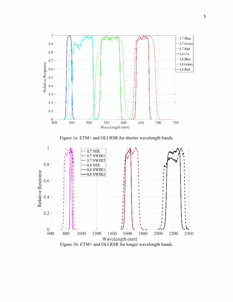
Figures 1a and 1b show the relative spectral responses (RSRs) for each band in the ETM+ and
OLI. The OLI RSRs are narrower and exhibit less variability in response across the passband than
the corresponding ETM+ RSRs. The OLI NIR band is shifted considerably towards the falling
edge of the ETM+ NIR band, and the OLI SWIR1 band is shifted towards the rising edge of the
ETM+ SWIR1 band. These changes to the OLI response were intended to reduce the sensitivity
of these bands to water vapor absorption.
The OLI has 2 additional bands the ETM+ does not: a Coastal/Aerosol band (approximately 430
to 450 nm) and a Cirrus band (approximately 1360 to 1380 nm). The Coastal/Aerosol band is
approximately centered on the rising edge of the ETM+ Blue band. As its name suggests, the
Coastal/Aerosol band is intended to measure atmospheric aerosols, while the Cirrus band is
intended to detect thin cirrus clouds. For the purposes of this work, the Cirrus band is not
considered further.
5
Figure 1a: ETM+ and OLI RSR for shorter wavelength bands.
Figure 1b: ETM+ and OLI RSR for longer wavelength bands.

6
CHAPTER 2
METHODOLOGY
This chapter discusses the methodology used to perform the analysis, beginning with the
procedure(s) used to select the test sites. The remainder of the chapter describes the characteristics
of the selected sites and the procedures used to perform the analysis.
2.1 Site Selection
The following criteria were used to guide the target site selection process:
• The target(s) should be as bright as possible. Reflectance measurements from brighter targets
have higher signal-to-noise ratios.
• The target(s) should exhibit low temporal and spatial uncertainty. This will help to ensure that
any changes measured by the sensor represent changes in the sensor response only
• Atmospheric measurements should be available for the target(s), and should come from an
operative weather station situated as close as possible to the target ROI. Atmospheric
measurements from stations close to the ROI should better represent the “true” condition of
the atmosphere over the ROI. There could be significant differences in atmospheric
measurements between the two locations.
Initially, PICS target(s) were considered in order to meet the first two criteria. From the set of
North African PICS studied by the Image Processing Laboratory, Libya-1 (WRS2 path/row
187/043), Libya-4 (WRS2 path/row 181/040), Niger-1 (WRS2 path/row 189/046), Niger-2 (WRS2
path/row 188/045), and Sudan-1 (WRS2 path/row 177/045) were chosen, as these demonstrated
the most temporal and spatial stability. Unfortunately, co-incident atmospheric measurements
7
from a nearby weather station were not available for these sites. Two alternative sites were selected
that had co-incident ground truth atmospheric measurements: (i) Algodones Dunes, CA (USA);
and (ii) a site near the city of Wadi ad-Dawasir, Saudi Arabia. Both sites are described below.
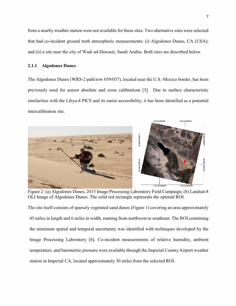
2.1.1 Algodones Dunes
The Algodones Dunes (WRS-2 path/row 039/037), located near the U.S.-Mexico border, has been
previously used for sensor absolute and cross calibrations [5]. Due to surface characteristic
similarities with the Libya-4 PICS and its easier accessibility, it has been identified as a potential
intercalibration site.
Figure 2: (a) Algodones Dunes, 2015 Image Processing Laboratory Field Campaign; (b) Landsat-8 OLI Image of Algodones Dunes. The solid red rectangle represents the optimal ROI. The site itself consists of sparsely vegetated sand dunes (Figure 1) covering an area approximately
45 miles in length and 6 miles in width, running from northwest to southeast. The ROI containing
the minimum spatial and temporal uncertainty was identified with techniques developed by the
Image Processing Laboratory [6]. Co-incident measurements of relative humidity, ambient
temperature, and barometric pressure were available through the Imperial County Airport weather
station in Imperial CA, located approximately 30 miles from the selected ROI.
8
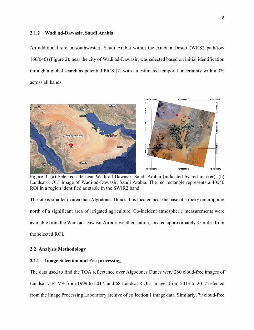
2.1.2 Wadi ad-Dawasir, Saudi Arabia
An additional site in southwestern Saudi Arabia within the Arabian Desert (WRS2 path/row
166/046) (Figure 2), near the city of Wadi ad-Dawasir, was selected based on initial identification
through a global search as potential PICS [7] with an estimated temporal uncertainty within 3%
across all bands.
Figure 3: (a) Selected site near Wadi ad-Dawasir, Saudi Arabia (indicated by red marker); (b) Landsat-8 OLI Image of Wadi-ad-Dawasir, Saudi Arabia. The red rectangle represents a 40x40 ROI in a region identified as stable in the SWIR2 band.
The site is smaller in area than Algodones Dunes. It is located near the base of a rocky outcropping
north of a significant area of irrigated agriculture. Co-incident atmospheric measurements were
available from the Wadi ad-Dawasir Airport weather station, located approximately 35 miles from
the selected ROI.
2.2 Analysis Methodology
2.2.1 Image Selection and Pre-processing
The data used to find the TOA reflectance over Algodones Dunes were 260 cloud-free images of
Landsat-7 ETM+ from 1999 to 2017, and 68 Landsat-8 OLI images from 2013 to 2017 selected
from the Image Processing Laboratory archive of collection 1 image data. Similarly, 79 cloud-free
9
Landsat-8 OLI images from 2013 to 2017 were selected for the Wadi ad-Dawasir site; ETM+
image data were not used in the analysis of this site as there was insufficient co-incident weather
station data available.
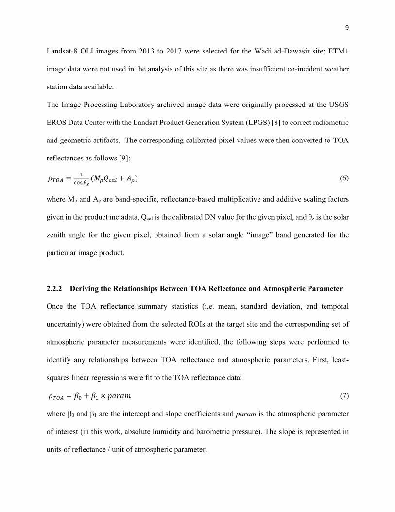
The Image Processing Laboratory archived image data were originally processed at the USGS
EROS Data Center with the Landsat Product Generation System (LPGS) [8] to correct radiometric
and geometric artifacts. The corresponding calibrated pixel values were then converted to TOA
reflectances as follows [9]:
𝜌𝜌𝑇𝑇𝑇𝑇𝑇𝑇 = 1cos𝜃𝜃𝑧𝑧
(𝑀𝑀𝜌𝜌𝑄𝑄𝑐𝑐𝑅𝑅𝑅𝑅 + 𝐴𝐴𝜌𝜌) (6)
where Mρ and Aρ are band-specific, reflectance-based multiplicative and additive scaling factors
given in the product metadata, Qcal is the calibrated DN value for the given pixel, and θz is the solar
zenith angle for the given pixel, obtained from a solar angle “image” band generated for the
particular image product.
2.2.2 Deriving the Relationships Between TOA Reflectance and Atmospheric Parameter
Once the TOA reflectance summary statistics (i.e. mean, standard deviation, and temporal
uncertainty) were obtained from the selected ROIs at the target site and the corresponding set of
atmospheric parameter measurements were identified, the following steps were performed to
identify any relationships between TOA reflectance and atmospheric parameters. First, least-
squares linear regressions were fit to the TOA reflectance data:
𝜌𝜌𝑇𝑇𝑇𝑇𝑇𝑇 = 𝛽𝛽0 + 𝛽𝛽1 × 𝑝𝑝𝑝𝑝𝑝𝑝𝑝𝑝𝑝𝑝 (7)
where β0 and β1 are the intercept and slope coefficients and param is the atmospheric parameter
of interest (in this work, absolute humidity and barometric pressure). The slope is represented in
units of reflectance / unit of atmospheric parameter.
10
The significance of the regression slopes was then tested using a two-sided hypothesis test at the
0.05 significance level. If the p-value of the test was greater than 0.05, there was insufficient
evidence to reject the null hypothesis of zero slope. If the p-value of the test was less than or equal
to 0.05, there was sufficient evidence to reject the null hypothesis and conclude a (statistically
significant, at least) relationship between TOA reflectance and the given atmospheric parameter
existed.
For those bands exhibiting sufficient statistical evidence to reject the null hypothesis of zero slope,
additional processing was performed to determine whether a linear function of atmospheric
parameter adequately accounted for the observed TOA reflectance behavior. This additional
processing is described in the following sections.
2.2.3 Consideration of Higher-Order and/or Nonlinear Atmospheric Parameter Models
In addition to linear functions of a single atmospheric parameter, higher-order and nonlinear
functions of a single atmospheric parameter were also considered. For each model tested, the R2
value was calculated to estimate the goodness of the model fit. The model having the highest R2
value was selected as the “optimal” model, and used to normalize the initial TOA reflectance data
as follows:
𝜌𝜌𝑐𝑐𝑐𝑐𝑐𝑐𝑐𝑐 = 𝜌𝜌𝑜𝑜𝑜𝑜𝑊𝑊𝜌𝜌𝑚𝑚𝑜𝑜𝑚𝑚𝑚𝑚𝑙𝑙
× 𝜌𝜌𝑐𝑐𝑜𝑜𝑤𝑤������ (8)
where ρobs is the observed TOA reflectance, ρmodel is the predicted TOA reflectance accounting for
the given atmospheric parameter(s), and 𝜌𝜌𝑐𝑐𝑜𝑜𝑤𝑤������ is the temporal mean of the observed TOA
reflectance. The normalized TOA reflectances were then replotted to check whether the temporal
uncertainty (i.e. the “spread” in the set of data points) was reduced after the correction.

11
2.2.4 BRDF Normalization
Typical analyses of desert site image data have used large areas (on the order of several hundred
km2) in order to minimize BRDF effects [10]. Since the optimal regions used in this work tend to
be much smaller in area, BRDF effects due to variation in solar position and/or sensor viewing
position throughout the year cannot be ignored.
For the Algodones Dunes site, a two-angle quadratic BRDF model was used:
𝜌𝜌𝐵𝐵𝑅𝑅𝐵𝐵𝐵𝐵 = 𝛽𝛽0 + 𝛽𝛽1𝑥𝑥12 + 𝛽𝛽2𝑦𝑦12 + 𝛽𝛽3𝑥𝑥1𝑦𝑦1 (9)
For the Wadi ad-Dawasir site, a four-angle linear BRDF model was used:
𝜌𝜌𝐵𝐵𝑅𝑅𝐵𝐵𝐵𝐵 = 𝛽𝛽0 + 𝛽𝛽1𝑥𝑥1 + 𝛽𝛽2𝑦𝑦1 + 𝛽𝛽3𝑥𝑥2 + 𝛽𝛽4𝑦𝑦2 (10)
For both models, x1, x2, y1, and y2 are the plane Cartesian coordinate values transformed from the
solar position zenith/azimuth angles (SZA, SAA) and sensor viewing zenith/azimuth angles (VZA,
VAA) based in a spherical coordinate system.
𝑥𝑥1 = sin(𝑆𝑆𝑆𝑆𝐴𝐴) cos(𝑆𝑆𝐴𝐴𝐴𝐴) (11a)
𝑦𝑦1 = sin(𝑆𝑆𝑆𝑆𝐴𝐴) sin(𝑆𝑆𝐴𝐴𝐴𝐴) (11b)
𝑥𝑥2 = sin(𝑉𝑉𝑆𝑆𝐴𝐴) cos(𝑉𝑉𝐴𝐴𝐴𝐴) (11c)
𝑦𝑦2 = sin(𝑉𝑉𝑆𝑆𝐴𝐴) sin(𝑉𝑉𝐴𝐴𝐴𝐴) (11d)
12
CHAPTER 3
RESULTS
This chapter presents the results of the analysis methodology given in the previous chapter. Results
for normalization using the “optimal” atmospheric parameter model are presented only for those
bands demonstrating a statistically significant linear relationship between TOA reflectance and the
atmospheric parameter of interest. The results for each sensor are presented according to site; the
results for absolute humidity are presented first, followed by the results for barometric pressure.
3.1 Algodones Dunes
3.1.1 Relationship Between TOA Reflectance and Absolute Humidity—Landsat 7 ETM+
NIR Band:
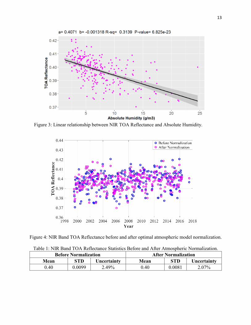
Figure 3 shows the relationship between TOA reflectance and absolute humidity for the NIR band.
The slope of the regression line was found to be strongly statistically significant (p-value =
approximately 6.83x10⁻²³ at the 0.05 significance level) and, as expected, indicated a negative
relationship between TOA reflectance and absolute humidity. The linear model accounted for
approximately 31.4% of the variability in the TOA reflectance.
The optimal atmospheric parameter model was found to be the initial linear model:
𝜌𝜌𝑚𝑚𝑐𝑐𝑚𝑚𝑅𝑅𝑅𝑅 = 0.4071 − 0.001318 × 𝐴𝐴𝑅𝑅 (12)
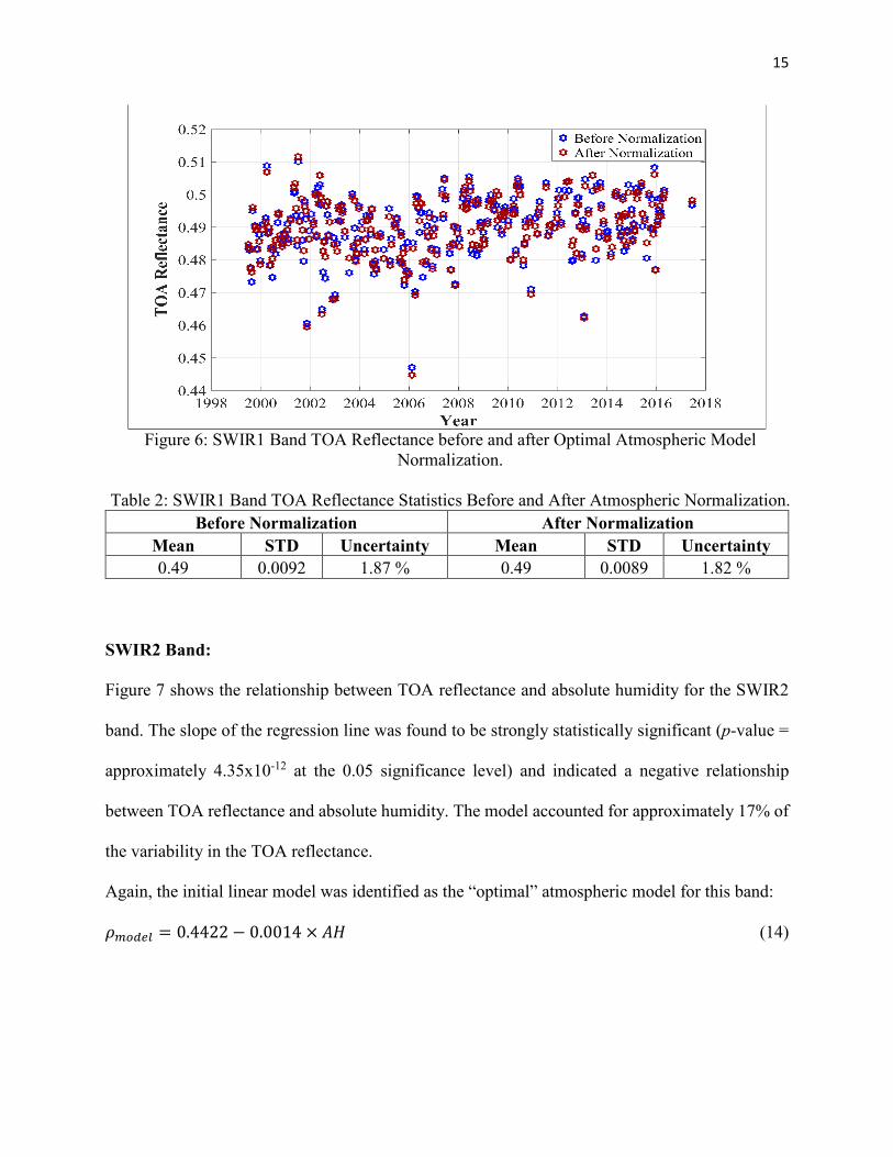
Figure 4 shows the resulting normalization provided with this model. The figure indicates that
after normalization the overall “spread” in the data was reduced. The reflectances of a few data
points (e.g. the early 2006 acquisition), however, appeared to be reduced further away from the
TOA reflectance mean. Table 1 shows the resulting statistics before and after normalization with
the atmospheric model. Clearly, the temporal uncertainty was reduced by the normalization.
13
Figure 3: Linear relationship between NIR TOA Reflectance and Absolute Humidity.
Figure 4: NIR Band TOA Reflectance before and after optimal atmospheric model normalization.
Table 1: NIR Band TOA Reflectance Statistics Before and After Atmospheric Normalization. Before Normalization After Normalization
Mean STD Uncertainty Mean STD Uncertainty 0.40 0.0099 2.49% 0.40 0.0081 2.07%

14
SWIR1 Band:
Figure 5 shows the relationship between TOA reflectance and absolute humidity in the SWIR1
band. The regression slope was found to be statistically significant (p-value = approximately
3.28x10⁻⁴ at the 0.05 significance level), and indicated the negative relationship between TOA
reflectance and absolute humidity. The model accounted for approximately 4.89% of the
variability in the TOA reflectance.
As in the NIR band, the “optimal” atmospheric parameter model was found to be the initial linear
model:
𝜌𝜌𝑚𝑚𝑐𝑐𝑚𝑚𝑅𝑅𝑅𝑅 = 0.4936 − 0.0005 × 𝐴𝐴𝑅𝑅 (13)
Figure 6 shows the resulting normalization provided with this model. As suggested by the low R2
value, the normalization had little apparent effect on the overall data spread. This can also be
observed in Table 2, where the temporal uncertainty shows only a slight reduction.
Figure 5: Linear Relationship between SWIR1 TOA Reflectance and Absolute Humidity.
15
Figure 6: SWIR1 Band TOA Reflectance before and after Optimal Atmospheric Model
Normalization.
Table 2: SWIR1 Band TOA Reflectance Statistics Before and After Atmospheric Normalization. Before Normalization After Normalization
Mean STD Uncertainty Mean STD Uncertainty 0.49 0.0092 1.87 % 0.49 0.0089 1.82 %
SWIR2 Band:
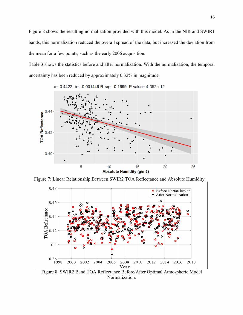
Figure 7 shows the relationship between TOA reflectance and absolute humidity for the SWIR2
band. The slope of the regression line was found to be strongly statistically significant (p-value =
approximately 4.35x10⁻¹² at the 0.05 significance level) and indicated a negative relationship
between TOA reflectance and absolute humidity. The model accounted for approximately 17% of
the variability in the TOA reflectance.
Again, the initial linear model was identified as the “optimal” atmospheric model for this band:
𝜌𝜌𝑚𝑚𝑐𝑐𝑚𝑚𝑅𝑅𝑅𝑅 = 0.4422 − 0.0014 × 𝐴𝐴𝑅𝑅 (14)
16
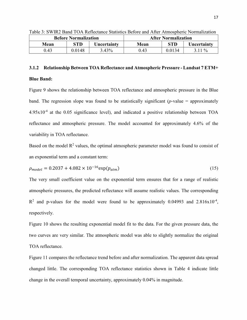
Figure 8 shows the resulting normalization provided with this model. As in the NIR and SWIR1
bands, this normalization reduced the overall spread of the data, but increased the deviation from
the mean for a few points, such as the early 2006 acquisition.
Table 3 shows the statistics before and after normalization. With the normalization, the temporal
uncertainty has been reduced by approximately 0.32% in magnitude.
Figure 7: Linear Relationship Between SWIR2 TOA Reflectance and Absolute Humidity.
Figure 8: SWIR2 Band TOA Reflectance Before/After Optimal Atmospheric Model
Normalization.
17
Table 3: SWIR2 Band TOA Reflectance Statistics Before and After Atmospheric Normalization Before Normalization After Normalization
Mean STD Uncertainty Mean STD Uncertainty 0.43 0.0148 3.43% 0.43 0.0134 3.11 %
3.1.2 Relationship Between TOA Reflectance and Atmospheric Pressure - Landsat 7 ETM+
Blue Band:
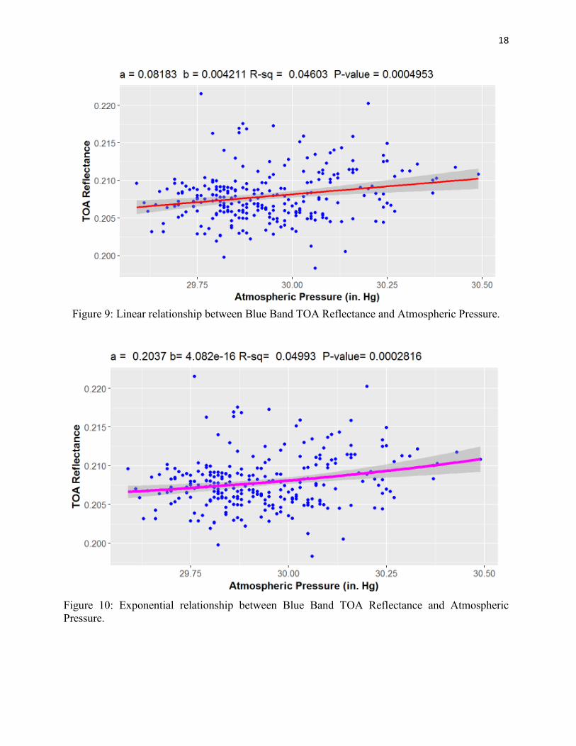
Figure 9 shows the relationship between TOA reflectance and atmospheric pressure in the Blue
band. The regression slope was found to be statistically significant (p-value = approximately
4.95x10⁻⁴ at the 0.05 significance level), and indicated a positive relationship between TOA
reflectance and atmospheric pressure. The model accounted for approximately 4.6% of the
variability in TOA reflectance.
Based on the model R2 values, the optimal atmospheric parameter model was found to consist of
an exponential term and a constant term:
𝜌𝜌𝑚𝑚𝑐𝑐𝑚𝑚𝑅𝑅𝑅𝑅 = 0.2037 + 4.082 × 10⁻¹⁶exp (𝑝𝑝𝑅𝑅𝑎𝑎𝑚𝑚) (15)
The very small coefficient value on the exponential term ensures that for a range of realistic
atmospheric pressures, the predicted reflectance will assume realistic values. The corresponding
R2 and p-values for the model were found to be approximately 0.04993 and 2.816x10⁻⁴,
respectively.
Figure 10 shows the resulting exponential model fit to the data. For the given pressure data, the
two curves are very similar. The atmospheric model was able to slightly normalize the original
TOA reflectance.
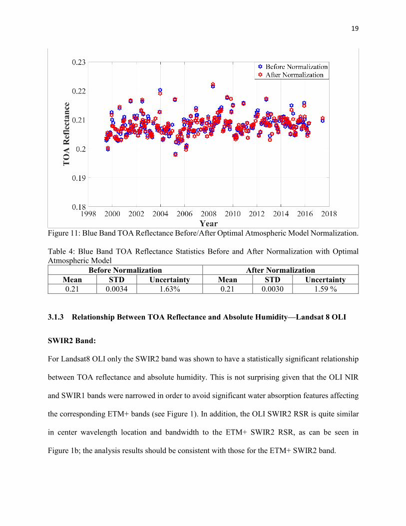
Figure 11 compares the reflectance trend before and after normalization. The apparent data spread
changed little. The corresponding TOA reflectance statistics shown in Table 4 indicate little
change in the overall temporal uncertainty, approximately 0.04% in magnitude.
18
Figure 9: Linear relationship between Blue Band TOA Reflectance and Atmospheric Pressure.
Figure 10: Exponential relationship between Blue Band TOA Reflectance and Atmospheric Pressure.
19
Figure 11: Blue Band TOA Reflectance Before/After Optimal Atmospheric Model Normalization.
Table 4: Blue Band TOA Reflectance Statistics Before and After Normalization with Optimal Atmospheric Model
Before Normalization After Normalization Mean STD Uncertainty Mean STD Uncertainty 0.21 0.0034 1.63% 0.21 0.0030 1.59 %
3.1.3 Relationship Between TOA Reflectance and Absolute Humidity—Landsat 8 OLI
SWIR2 Band:
For Landsat8 OLI only the SWIR2 band was shown to have a statistically significant relationship
between TOA reflectance and absolute humidity. This is not surprising given that the OLI NIR
and SWIR1 bands were narrowed in order to avoid significant water absorption features affecting
the corresponding ETM+ bands (see Figure 1). In addition, the OLI SWIR2 RSR is quite similar
in center wavelength location and bandwidth to the ETM+ SWIR2 RSR, as can be seen in
Figure 1b; the analysis results should be consistent with those for the ETM+ SWIR2 band.
20
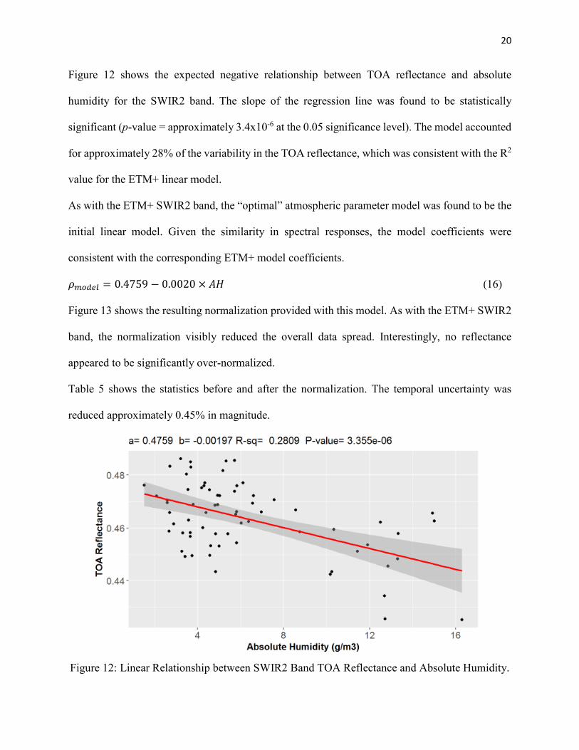
Figure 12 shows the expected negative relationship between TOA reflectance and absolute
humidity for the SWIR2 band. The slope of the regression line was found to be statistically
significant (p-value = approximately 3.4x10⁻⁶ at the 0.05 significance level). The model accounted
for approximately 28% of the variability in the TOA reflectance, which was consistent with the R2
value for the ETM+ linear model.
As with the ETM+ SWIR2 band, the “optimal” atmospheric parameter model was found to be the
initial linear model. Given the similarity in spectral responses, the model coefficients were
consistent with the corresponding ETM+ model coefficients.
𝜌𝜌𝑚𝑚𝑐𝑐𝑚𝑚𝑅𝑅𝑅𝑅 = 0.4759 − 0.0020 × 𝐴𝐴𝑅𝑅 (16)
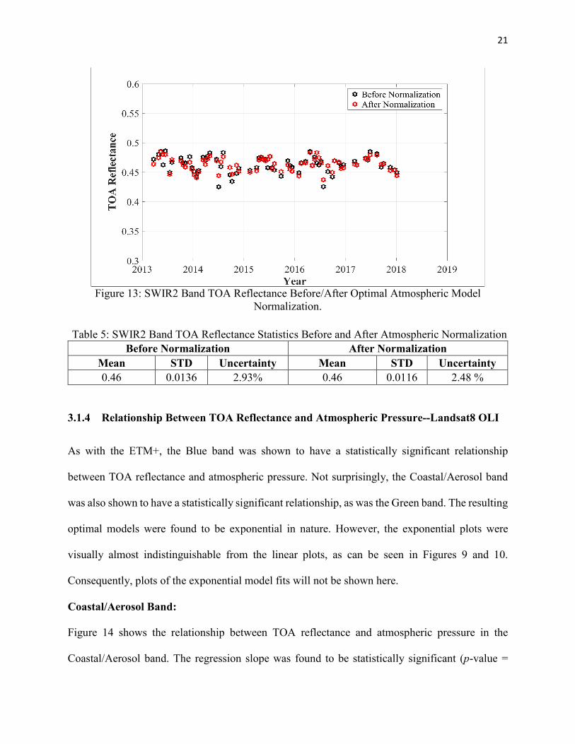
Figure 13 shows the resulting normalization provided with this model. As with the ETM+ SWIR2
band, the normalization visibly reduced the overall data spread. Interestingly, no reflectance
appeared to be significantly over-normalized.
Table 5 shows the statistics before and after the normalization. The temporal uncertainty was
reduced approximately 0.45% in magnitude.
Figure 12: Linear Relationship between SWIR2 Band TOA Reflectance and Absolute Humidity.
21
Figure 13: SWIR2 Band TOA Reflectance Before/After Optimal Atmospheric Model
Normalization. Table 5: SWIR2 Band TOA Reflectance Statistics Before and After Atmospheric Normalization
Before Normalization After Normalization Mean STD Uncertainty Mean STD Uncertainty 0.46 0.0136 2.93% 0.46 0.0116 2.48 %
3.1.4 Relationship Between TOA Reflectance and Atmospheric Pressure--Landsat8 OLI
As with the ETM+, the Blue band was shown to have a statistically significant relationship
between TOA reflectance and atmospheric pressure. Not surprisingly, the Coastal/Aerosol band
was also shown to have a statistically significant relationship, as was the Green band. The resulting
optimal models were found to be exponential in nature. However, the exponential plots were
visually almost indistinguishable from the linear plots, as can be seen in Figures 9 and 10.
Consequently, plots of the exponential model fits will not be shown here.
Coastal/Aerosol Band:
Figure 14 shows the relationship between TOA reflectance and atmospheric pressure in the
Coastal/Aerosol band. The regression slope was found to be statistically significant (p-value =

22
approximately 4.97x10⁻⁵ at the 0.05 significance level), and indicated a positive relationship
between TOA reflectance and atmospheric pressure. The model accounted for approximately
22.2% of the variability in TOA reflectance.
Based on the model R2 values, the optimal atmospheric parameter model was found to consist of
an exponential term and a constant term. The R2 and p-value for this model were found to be
approximately 0.02239 and 4.6×10⁻⁵ respectively.
𝜌𝜌𝑚𝑚𝑐𝑐𝑚𝑚𝑅𝑅𝑅𝑅 = 0.1982 + 1.002 × 10⁻¹⁵exp (𝑝𝑝𝑅𝑅𝑎𝑎𝑚𝑚) (17)
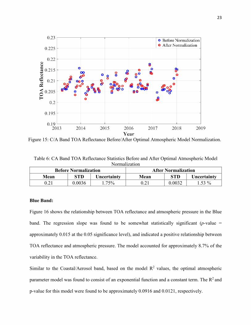
Figure 15 shows the trend comparison before and after normalization. It can be seen that the
atmospheric model was able to normalize the original TOA reflectance significantly. However,
some of the lower reflectance data points, such as the two acquisitions in early 2017, were reduced
further away from the overall reflectance mean.
Table 6 shows the statistics before and after normalization using atmospheric model. It can be
noticed that the temporal uncertainty was reduced by approximately 0.22% in magnitude.
Figure 14: Linear Relationship between C/A Band TOA Reflectance and Atmospheric Pressure.
23
Figure 15: C/A Band TOA Reflectance Before/After Optimal Atmospheric Model Normalization.
Table 6: CA Band TOA Reflectance Statistics Before and After Optimal Atmospheric Model Normalization
Before Normalization After Normalization Mean STD Uncertainty Mean STD Uncertainty 0.21 0.0036 1.75% 0.21 0.0032 1.53 %
Blue Band:
Figure 16 shows the relationship between TOA reflectance and atmospheric pressure in the Blue
band. The regression slope was found to be somewhat statistically significant (p-value =
approximately 0.015 at the 0.05 significance level), and indicated a positive relationship between
TOA reflectance and atmospheric pressure. The model accounted for approximately 8.7% of the
variability in the TOA reflectance.
Similar to the Coastal/Aerosol band, based on the model R2 values, the optimal atmospheric
parameter model was found to consist of an exponential function and a constant term. The R2 and
p-value for this model were found to be approximately 0.0916 and 0.0121, respectively.

24
𝜌𝜌𝑚𝑚𝑐𝑐𝑚𝑚𝑅𝑅𝑅𝑅 = 0.2084 + 4.988 × 10⁻¹⁶exp (𝑝𝑝𝑅𝑅𝑎𝑎𝑚𝑚) (18)
Figure 17 shows the trend comparison before and after normalization. Not surprisingly, the overall
uncertainty (Table 7) was reduced by approximately 0.07% in magnitude, a slight change.
Figure 16: Linear Relationship Between Blue Band TOA Reflectance and Atmospheric Pressure.
Figure 17: Blue Band TOA Reflectance Before/After Optimal Atmospheric Model Normalization.

25
Table 7: Blue Band TOA Reflectance Statistics Before and After Optimal Atmospheric Model Normalization
Before Normalization After Normalization Mean STD Uncertainty Mean STD Uncertainty 0.21 0.0028 1.33% 0.21 0.0027 1.26 %
Green Band:
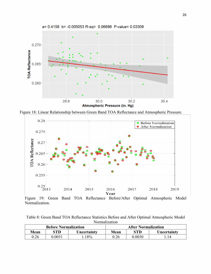
Figure 18 shows the relationship between TOA reflectance and atmospheric pressure in the Green
band. The regression slope was found to be marginally statistically significant (p-value =
approximately 0.033 at the 0.05 significance level), and indicated a negative relationship between
TOA reflectance and atmospheric pressure. The model accounted for approximately 6.7% of the
variability in TOA reflectance.
The “optimal” atmospheric model consisted of a constant term and an exponential term. The R2
and p-value for this model were found to be approximately 0.0723 and 0.031, respectively--slightly
better than the linear model.
𝜌𝜌𝑚𝑚𝑐𝑐𝑚𝑚𝑅𝑅𝑅𝑅 = 0.2689 − 4.327 × 10⁻¹⁶exp (𝑝𝑝𝑅𝑅𝑎𝑎𝑚𝑚) (19)
Figure 19 shows the trend comparison before and after normalization. The atmospheric model was
able to slightly normalize the original TOA reflectance.
Table 8 shows the statistics before and after normalization using atmospheric model. It can be
noticed that the overall uncertainty was reduced by approximately 0.04% in magnitude, a slight
change.
26
Figure 18: Linear Relationship between Green Band TOA Reflectance and Atmospheric Pressure.
Figure 19: Green Band TOA Reflectance Before/After Optimal Atmospheric Model Normalization.
Table 8: Green Band TOA Reflectance Statistics Before and After Optimal Atmospheric Model Normalization
Before Normalization After Normalization Mean STD Uncertainty Mean STD Uncertainty 0.26 0.0031 1.18% 0.26 0.0030 1.14
27
3.2 Wadi ad-Dawasir Desert Site
This section presents the characterization results obtained for the Wadi ad-Dawasir site. Only the
results for the OLI are presented, as there was insufficient weather station data available to allow
a similar analysis for the ETM+.
3.2.1 Relationship Between TOA Reflectance and Absolute Humidity
Figure 20 shows the relationship between TOA reflectance and absolute humidity for the SWIR2
band. The slope of the regression line was found to be statistically significant (p-value =
approximately 3.27x10⁻³ at the 0.05 significance level) and indicated a negative relationship
between TOA reflectance and absolute humidity. The model accounted for approximately 10.7%
of the variability in the TOA reflectance.
As in the SWIR2 band, the “optimal” atmospheric parameter model was found to be the initial
linear model:
𝜌𝜌𝑚𝑚𝑐𝑐𝑚𝑚𝑅𝑅𝑅𝑅 = 0.4696 − 0.0014 × 𝐴𝐴𝑅𝑅 (20)
Figure 21 shows the resulting normalization provided with this model. The normalization visibly
reduced the overall spread of the data. Reflectances for some of the data points, such as the early
2017 acquisition, appeared to be over normalized.
Table 9 shows the statistics before and after normalization using atmospheric model. The overall
uncertainty was reduced by approximately 0.16% in magnitude.

28
Figure 20: Linear Relationship Between SWIR2 Band TOA Reflectance and Absolute Humidity.
Figure 21: SWIR2 Band TOA Reflectance Before/After Optimal Atmospheric Model Normalization.
Table 9: SWIR2 Band TOA Reflectance Statistics Before and After Atmospheric Normalization Before Normalization After Normalization
Mean STD Uncertainty Mean STD Uncertainty 0.45 0.0130 2.88% 0.46 0.0116 2.72 %

29
3.2.2 Relationship Between TOA Reflectance and Atmospheric Pressure
Coastal/Aerosol Band:
Figure 22 shows the relationship between TOA reflectance and atmospheric pressure in the
Coastal/Aerosol band. The regression slope was found to be marginally statistically significant (p-
value = approximately 0.043 at the 0.05 significance level), and, interestingly, indicated a negative
relationship between TOA reflectance and atmospheric pressure. The model accounted for
approximately 5.2% of the variability in the TOA reflectance.
The “optimal” atmospheric parameter model for this band consisted of an exponential term and a
constant term. The R2 and p-value for this model were found to be 0.0537 and 0.0391 respectively.
𝜌𝜌𝑚𝑚𝑐𝑐𝑚𝑚𝑅𝑅𝑅𝑅 = 0.2151 − 7.283 × 10⁻¹⁶exp (𝑝𝑝𝑅𝑅𝑎𝑎𝑚𝑚) (21)
Figure 23 shows the trend comparison before and after normalization. The observed data spread
was slightly reduced. However, no data points appeared to be significantly over-normalized. The
corresponding uncertainty, as shown in Table 10, was reduced by approximately 0.06% in
magnitude.
Figure 22: Linear Relationship Between C/A TOA Reflectance and Atmospheric Pressure.

30
Figure 23: C/A Band TOA Reflectance Before/After Optimal Atmospheric Model Normalization.
Table 10: Coastal/Aerosol Band TOA Reflectance Statistics Before and After Optimal Atmospheric Model Normalization.
Before Normalization After Normalization Mean STD Uncertainty Mean STD Uncertainty 0.21 0.0060 2.88% 0.21 0.0058 2.82 %
Blue Band:
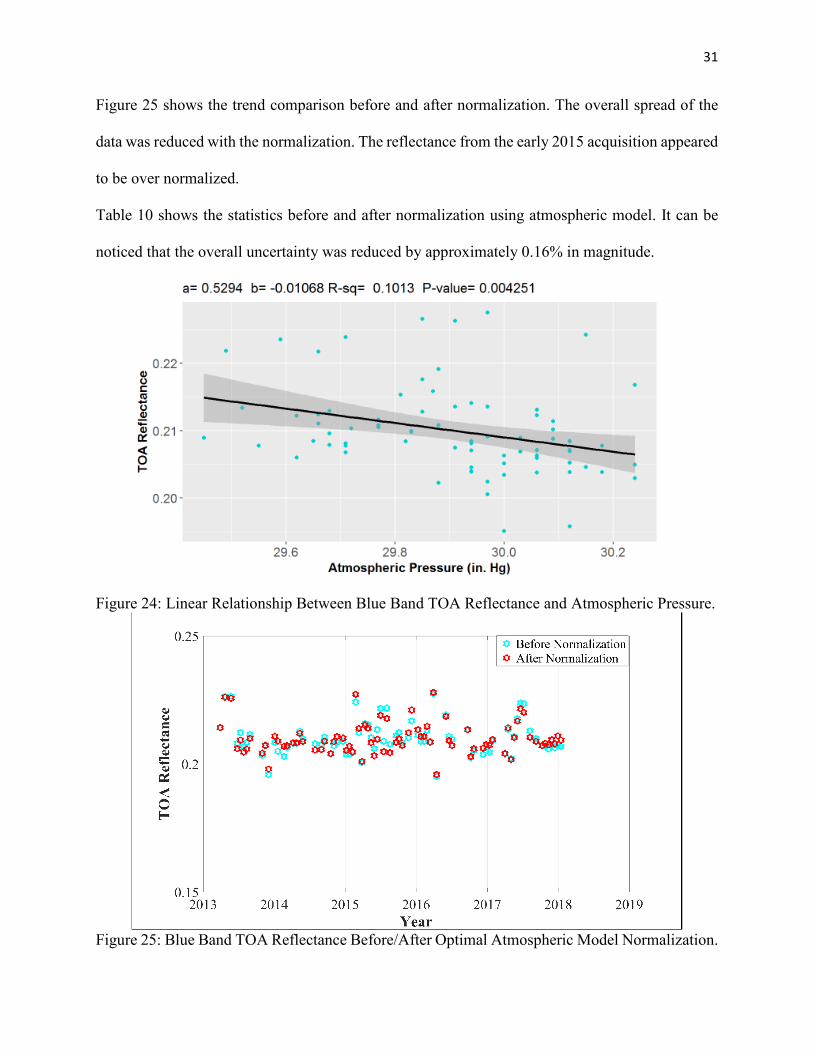
Figure 24 shows the relationship between TOA reflectance and atmospheric pressure in the Blue
band. The regression slope was found to be statistically significant (p-value = approximately
4.25x10⁻³ at the 0.05 significance level), and indicated a negative relationship between TOA
reflectance and atmospheric pressure. The model accounted for approximately 10.1% of the
variability in TOA reflectance.
The “optimal” atmospheric model consisted of an exponential term and a constant term. The R2
and p-value for this model were found to be 0.1014 and 0.0042, respectively.
𝜌𝜌𝑚𝑚𝑐𝑐𝑚𝑚𝑅𝑅𝑅𝑅 = 0.2210 − 1.113 × 10⁻¹⁵exp (𝑝𝑝𝑅𝑅𝑎𝑎𝑚𝑚) (22)
31
Figure 25 shows the trend comparison before and after normalization. The overall spread of the
data was reduced with the normalization. The reflectance from the early 2015 acquisition appeared
to be over normalized.
Table 10 shows the statistics before and after normalization using atmospheric model. It can be
noticed that the overall uncertainty was reduced by approximately 0.16% in magnitude.
Figure 24: Linear Relationship Between Blue Band TOA Reflectance and Atmospheric Pressure.
Figure 25: Blue Band TOA Reflectance Before/After Optimal Atmospheric Model Normalization.

32
Table 11: Blue Band TOA Reflectance Statistics Before and After Optimal Atmospheric Model Normalization.
Before Normalization After Normalization Mean STD Uncertainty Mean STD Uncertainty 0.21 0.0064 3.08% 0.21 0.0061 2.92 %
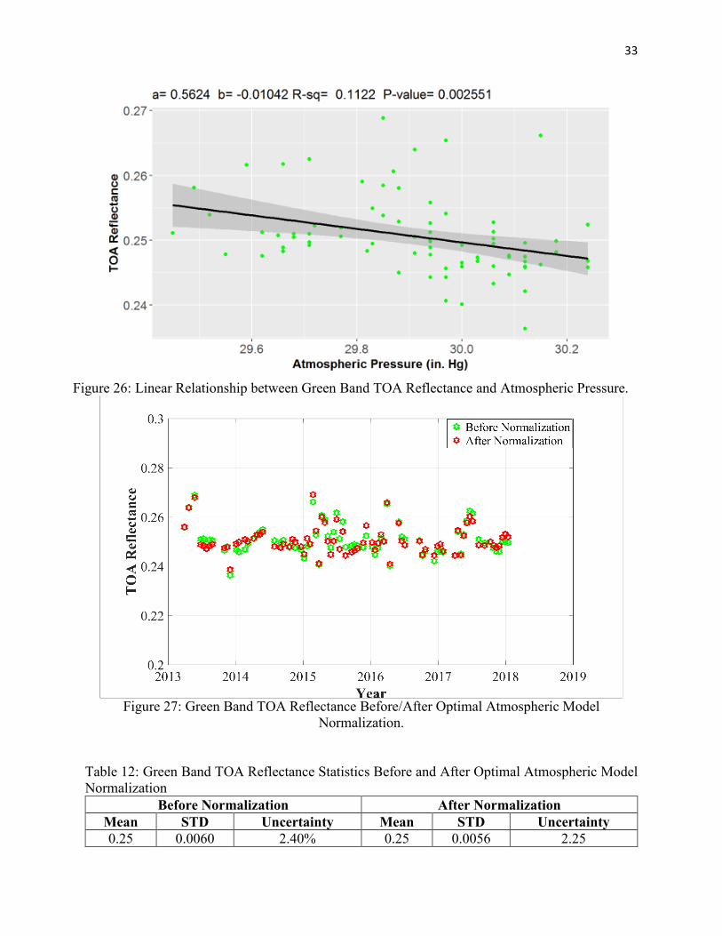
Green Band:
Figure 26 shows the relationship between TOA reflectance and atmospheric pressure in the Green
band. The regression slope was found to be statistically significant (p-value = approximately
2.55x10⁻³ at the 0.05 significance level), and indicated a negative relationship between TOA
reflectance and atmospheric pressure. The model accounted for approximately 11.2% of the
variability in TOA reflectance.
The “optimal” atmospheric model consisted of an exponential term and a constant term. The R2
and p-value for this model were found to be 0.1169 and 0.0020 respectively.
𝜌𝜌𝑚𝑚𝑐𝑐𝑚𝑚𝑅𝑅𝑅𝑅 = 0.2617 − 1.110 × 10⁻¹⁵exp (𝑝𝑝𝑅𝑅𝑎𝑎𝑚𝑚) (23)
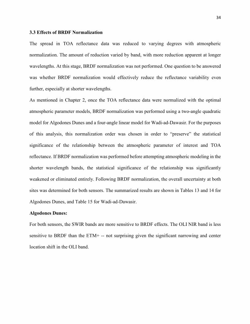
Figure 27 shows the trend comparison before and after normalization. Again, the overall data
spread was reduced with the normalization. The reflectance data from the acquisition in early 2015
appeared to be over-normalized in this band as well. The corresponding overall temporal
uncertainty was reduced by approximately 0.15% in magnitude, as shown in Table 12.
33
Figure 26: Linear Relationship between Green Band TOA Reflectance and Atmospheric Pressure.
Figure 27: Green Band TOA Reflectance Before/After Optimal Atmospheric Model
Normalization.
Table 12: Green Band TOA Reflectance Statistics Before and After Optimal Atmospheric Model Normalization
Before Normalization After Normalization Mean STD Uncertainty Mean STD Uncertainty 0.25 0.0060 2.40% 0.25 0.0056 2.25
34
3.3 Effects of BRDF Normalization
The spread in TOA reflectance data was reduced to varying degrees with atmospheric
normalization. The amount of reduction varied by band, with more reduction apparent at longer
wavelengths. At this stage, BRDF normalization was not performed. One question to be answered
was whether BRDF normalization would effectively reduce the reflectance variability even
further, especially at shorter wavelengths.
As mentioned in Chapter 2, once the TOA reflectance data were normalized with the optimal
atmospheric parameter models, BRDF normalization was performed using a two-angle quadratic
model for Algodones Dunes and a four-angle linear model for Wadi-ad-Dawasir. For the purposes
of this analysis, this normalization order was chosen in order to “preserve” the statistical
significance of the relationship between the atmospheric parameter of interest and TOA
reflectance. If BRDF normalization was performed before attempting atmospheric modeling in the
shorter wavelength bands, the statistical significance of the relationship was significantly
weakened or eliminated entirely. Following BRDF normalization, the overall uncertainty at both
sites was determined for both sensors. The summarized results are shown in Tables 13 and 14 for
Algodones Dunes, and Table 15 for Wadi-ad-Dawasir.
Algodones Dunes:
For both sensors, the SWIR bands are more sensitive to BRDF effects. The OLI NIR band is less
sensitive to BRDF than the ETM+ -- not surprising given the significant narrowing and center
location shift in the OLI band.

35
Table 13: TOA Reflectance Summary Statistics for ETM+ Bands After Atmospheric and BRDF Normalization.
Before Atmospheric Normalization
After Atmospheric Normalization
Uncertainty After BRDF
Normalization (%) Bands Mean STD Uncertainty
(%) Mean STD Uncertainty (%)
Blue 0.21 0.0034 1.63 0.21 0.0030 1.59 1.44
Green 0.26 0.0039 1.48 0.26 0.0039 1.48 1.36
Red 0.35 0.0056 1.59 0.35 0.0056 1.59 1.41
NIR 0.40 0.0099 2.49 0.40 0.0081 2.07 2.01
SWIR1 0.49 0.0092 1.87 0.49 0.0089 1.82 1.66
SWIR2 0.43 0.0148 3.43 0.43 0.0134 3.11 2.69
Table 14: TOA Reflectance Summary Statistics for OLI Bands After Atmospheric and BRDF Normalization.
Before Atmospheric Normalization
After Atmospheric Normalization
Uncertainty After BRDF
Normalization (%) Bands Mean STD Uncertainty
(%) Mean STD Uncertainty (%)
CA 0.21 0.0036 1.75 0.21 0.0032 1.53 1.14
Blue 0.21 0.0028 1.33 0.21 0.0027 1.26 0.97
Green 0.26 0.0031 1.18 0.26 0.0030 1.14 0.95
Red 0.35 0.0044 1.26 0.35 0.0044 1.26 1.00
NIR 0.43 0.0046 1.05 0.43 0.0046 1.05 0.92
SWIR1 0.50 0.0074 1.48 0.50 0.0074 1.48 0.90
SWIR2 0.46 0.0136 2.93 0.46 0.0116 2.48 1.87
Wadi ad-Dawasir:
36
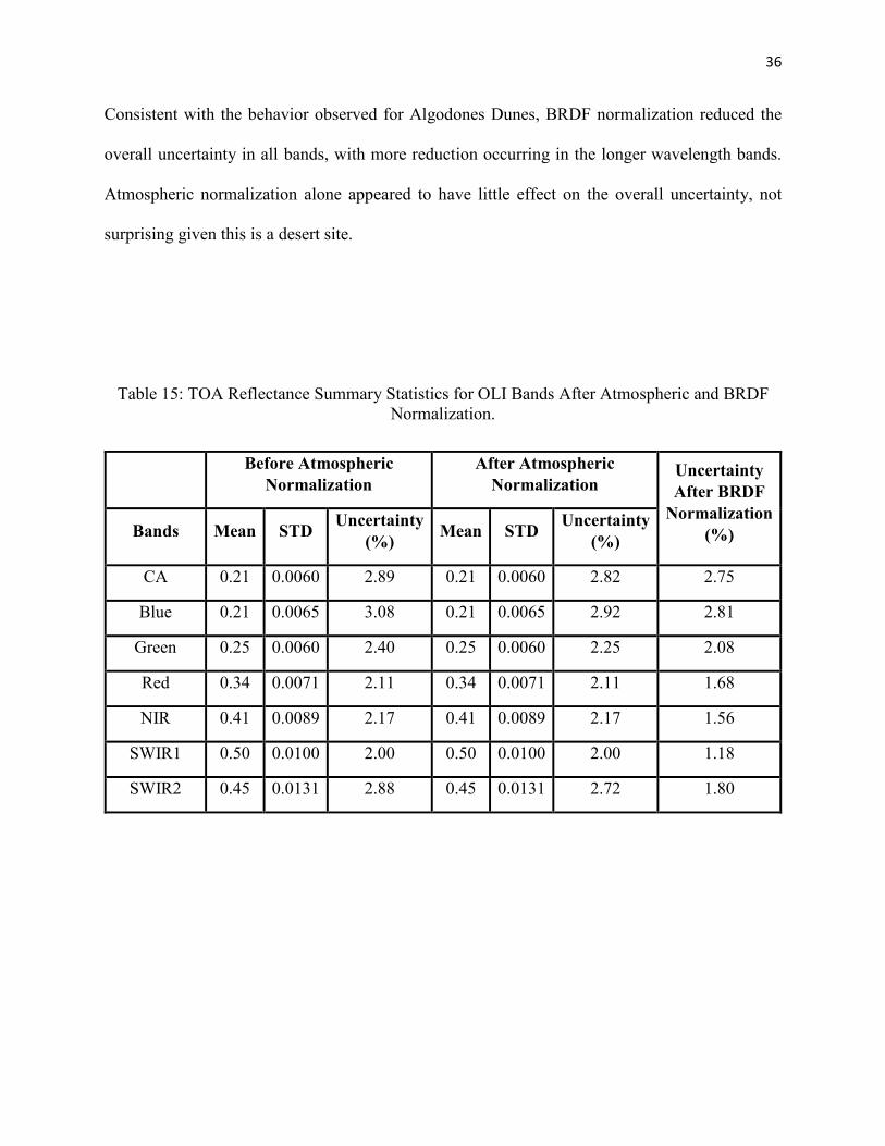
Consistent with the behavior observed for Algodones Dunes, BRDF normalization reduced the
overall uncertainty in all bands, with more reduction occurring in the longer wavelength bands.
Atmospheric normalization alone appeared to have little effect on the overall uncertainty, not
surprising given this is a desert site.
Table 15: TOA Reflectance Summary Statistics for OLI Bands After Atmospheric and BRDF Normalization.
Before Atmospheric Normalization
After Atmospheric Normalization
Uncertainty After BRDF
Normalization (%) Bands Mean STD Uncertainty
(%) Mean STD Uncertainty (%)
CA 0.21 0.0060 2.89 0.21 0.0060 2.82 2.75
Blue 0.21 0.0065 3.08 0.21 0.0065 2.92 2.81
Green 0.25 0.0060 2.40 0.25 0.0060 2.25 2.08
Red 0.34 0.0071 2.11 0.34 0.0071 2.11 1.68
NIR 0.41 0.0089 2.17 0.41 0.0089 2.17 1.56
SWIR1 0.50 0.0100 2.00 0.50 0.0100 2.00 1.18
SWIR2 0.45 0.0131 2.88 0.45 0.0131 2.72 1.80
37
CHAPTER 4
Conclusion and Future Directions
A new model was developed to characterize and normalize effects of atmospheric parameters on
TOA reflectance, using available ETM+/OLI image data and nearby weather station data acquired
for the Algodones Dunes and Wadi-ad-Dawasir sites. Moreover, according to the results presented
in Chapter 3, the following observations can be made:
• Atmospheric pressure was found to be significant at shorter wavelengths. This result is not
unexpected, as i) Rayleigh scattering at shorter wavelengths is greater, and Rayleigh scattering is
a function of atmospheric pressure; and ii) shorter wavelengths are more affected by atmospheric
aerosols. For Algodones Dunes, the relationship was positive for the ETM+ Blue and OLI
Coastal/Aerosol and Blue bands (increased TOA reflectance at higher atmospheric pressures). For
Wadi-ad-Dawasir, the relationship was negative in the OLI Coastal/Aerosol and Blue bands
(decreased TOA reflectance at higher atmospheric pressures); for both sites, the relationship was
38
negative in the OLI Green band. This was a surprising result for the Coastal/Aerosol and Blue
bands, suggesting a potential site dependence.
• Also, not surprisingly, water vapor was found to be significant at longer wavelengths, tending to
reduce TOA reflectance. This was found to be more of an issue with the ETM+ in the NIR and
SWIR1 bands, and with both sensors in the SWIR2 band. Again, this is not unexpected, as it
follows from each sensor’s observed spectral response.
• In all cases, linear models of atmospheric parameters accounted for less than 50% of the observed
variability in TOA reflectance, based on the estimated regression R2 values. Exponential models
for atmospheric pressure accounted for similarly low levels of variability.
• For Algodones Dunes, BRDF normalization after atmospheric normalization reduced the
uncertainty to within 2% for all ETM+ bands except SWIR2, whose uncertainty was reduced from
approximately 3.5% to approximately 2.7%. Similar normalizations reduced the uncertainty to
within 1% for all OLI bands except SWIR2, whose uncertainty was reduced to approximately 2%.
For the Wadi ad-Dawasir site, BRDF normalization reduced the uncertainty to within 2% for all
OLI bands except the Coastal/Aerosol and Blue bands. However, these figures should be
considered tentative pending additional characterization of each site.
4.1 Processing Recommendations
Based on the results obtained from this work, the following processing recommendations can be
made:
• Atmospheric parameter measurements should be acquired as close to the image acquisition time
as possible.

39
• Ground stations measuring surface humidity and atmospheric pressure should be as close as
possible to the test site.
• Locally accessible databases containing more temporally complete ground station information
should be developed.
• To provide maximum reduction in uncertainty, BRDF correction should be performed after
atmospheric correction.
4.2 Future Directions
This work could be extended in one or more of the following ways:
• Explore more stable sites throughout the world having nearby weather stations, so that those sites
would be useful for calibration purposes.
• Try to characterize the relationship between additional atmospheric parameters and TOA
reflectance at shorter wavelengths. Potential parameters for these bands would most likely be those
affecting aerosol characteristics, such as wind speed and/or visibility.
• Develop a “composite” model simultaneously accounting for atmospheric and BRDF effects.
40
References
[1] D. L. Helder, B. Basnet and D. Morstad, “Optimized identification of worldwide
radiometric pseudo-invariant calibration sites,” Canadian Journal of Remote Sensing, vol. 36,
pp. 527-539.
[2] D. Helder, J. Thome, N. Mishra, G. Chander, X. Xiong, A. Angal, and T. Choi, "Absolute
Calibration of Landsat Using a Pseudo Invariant Calibration Site", IEEE Trans. Geosci.
RemoteSens., vol. 51, no. 3, 2013.
[3] Wayne C. Turner, Steve Doty, “Energy Management Handbook”, 6th Ed., Lilburn, GA:
Fairmont Press, 2007, pp P1-P2.
[4] A.V. Kozak, V.G. Metlov, G.A. Terez and E.I. Terez, “On accounting for temperature and
pressure in determining the Rayleigh scattering in the earth’s atmosphere”, Bulletin of the
Crimean Astrophysical Observatory, June 2010, Volume 106, Issue 1, pp 87-91
[5] M M Farhad, “Cross calibration and validation of Landsat 8 OLI and Sentinel 2A MSI”,
Masters Graduate Thesis: South Dakota State University, 2018.
[6] H. Vuppula, “Normalization of pseudo-invariant calibration sites for increasing the
temporal resolution and long-term trending”, Masters Graduate Thesis: South Dakota State
University, 2017.
[7] R. Tabassum, “Worldwide optimal PICS search”, Masters Graduate Thesis: South Dakota
State University, 2017.

41
[8] https://landsat.usgs.gov/product-information.
[9] https://landsat.usgs.gov/using-usgs-landsat-8-product.
[10] H. Cosnefroy, M. Leroy, and X. Briottet, "Selection and characterization of Saharan and
Arabian desert sites for the calibration of optical satellite sensors," Remote Sensing of
Environment, vol. 58, pp. 101-114, 1996.