arX

iv:c

ond-

mat

/031

0061

v2 [

cond

-mat

.sta

t-m

ech]

27

Nov

200

3 Do Pareto-Zipf and Gibrat laws hold true?

An analysis with European Firms

Yoshi Fujiwara a,1 Corrado Di Guilmi b Hideaki Aoyama c

Mauro Gallegati b Wataru Souma a

aATR Human Information Science Laboratories, Kyoto 619-0288, Japan

bDepartment of Economics, Universita Politecnica delle Marche, P. Martelli 8,I-62100 Ancona, Italy

cGraduate School of Science, Kyoto University, Kyoto 606-8501, Japan

Abstract

By employing exhaustive lists of large firms in European countries, we show thatthe upper-tail of the distribution of firm size can be fitted with a power-law (Pareto-Zipf law), and that in this region the growth rate of each firm is independent of thefirm’s size (Gibrat’s law of proportionate effect). We also find that detailed balanceholds in the large-size region for periods we investigated; the empirical probabilityfor a firm to change its size from a value to another is statistically the same asthat for its reverse process. We prove several relationships among Pareto-Zipf’s law,Gibrat’s law and the condition of detailed balance. As a consequence, we show thatthe distribution of growth rate possesses a non-trivial relation between the positiveside of the distribution and the negative side, through the value of Pareto index, asis confirmed empirically.

Key words: Pareto-Zipf law, Gibrat law, firm growth, detailed balance,EconophysicsPACS: 89.90.+n, 02.50.-r, 05.40.+j, 47.53.+n

1 Introduction

Pareto [1] is generally credited with the discovery, more than a century ago,that the distribution of personal income obeys a power-law in high-income

Email address: yfujiwar@atr.co.jp (Yoshi Fujiwara).1 Corresponding author. FAX: +81-774-95-2647.

Preprint submitted to Elsevier Science 1 November 2018

range 2 . Firm size also has a skew distribution [3], and quite often obeys apower-law in the upper tail of the distribution. In terms of cumulative distri-bution P>(x) for firm size x, this states that

P>(x) ∝ x−µ, (1)

for large x, with µ being a parameter called Pareto index. The special caseµ = 1 is often referred to as Zipf’s law [4]. In this paper we call it Pareto-Zipflaw, the fact that firm size has a power-law distribution asymptotically forlarge firms.

Even if the range for which eq. (1) is valid is a few percent in the upper tail ofthe distribution, it is often observed that such a small fraction of firms occupiesa large amount of total sum of firm sizes. This means that a small idiosyncraticshock can make a considerable macro-economic impact. It is, therefore, quiteimportant to ask what is the underlying dynamics that governs the growth ofthose large firms.

Let a firm’s size be x1 at a time and x2 at a later time. Growth rate R isdefined as the ratio R = x2/x1. Law of proportionate effect [5] (see also [6]) isa postulate that the growth rate of a firm is independent of the firm’s attainedsize, i.e.

P (R|x1) is independent of x1, (2)

where P (R|x) is the probability distribution of growth rate conditional on theinitial size x1. In this paper we call this assumption as Gibrat’s law 3 .

These two laws have been extensively studied in industrial organization andrelated stochastic models [3,6,9,10,11,12,13,14,15,16,17,18,19,20,21,22,23,24](see [25] for review). Recent study in econophysics [26,27,28,29,30,31,32,33,34,35,36,37]introduced some notions and concepts of statistical physics into economics (see[38]). Present status related to firm-size growth may be summarized as follows.Firm size distribution is approximately log-normal with deviation from it inthe upper tail of the distribution (e.g. [24] for recent data). On the other hand,Gibrat’s law breaks down in the sense that the fluctuations of growth rate scaleas a power-law with firm size; smaller firms can possibly have larger fluctu-ations (e.g. [27,28]). However, little attention has been paid to the regimeof firm size where power-law is dominant rather than log-normality, and tothe validity of Gibrat’s law in that regime. More importantly, any kinematic

2 See [2] for modern and high-quality personal-income data in Japan.3 Another interesting and related quantity is flow, e.g. profits, rather than stock.See [7] for growth of individual personal-income and [8] for firms tax-income growth,and validity of Gibrat’s law.

2

relationship between Pareto-Zipf and Gibrat laws has not been understoodexplicitly, although there have been a lot of works on stochastic dynamicssince Gibrat. This issue is exactly what the present paper addresses.

For our purpose it is crucial to employ exhaustive lists of large firms. Ourdataset for European countries is exhaustive in the sense that each list includesall the active firms in each country whose sizes exceed a certain thresholdof observation. We show that both of the Pareto-Zipf law and Gibrat’s lawdo hold for those large firms. As our main result, we prove that Pareto-Zipflaw implies Gibrat’s law and vice versa under detailed balance. By showingthat the condition of detailed balance also holds in our empirical data, wecan show the equivalence of Pareto-Zipf law and Gibrat’s law as a kinematicprinciple in firms growth, irrespective of the underlying dynamics. Thereby, weconjecture that Gibrat’s law does hold in the regime of Pareto-Zipf for largefirms, but does not for smaller firms. Thus our result is not contradictory to thebreakdown of Gibrat’s law in previous study, most notably to the recent workby Stanley’s group [27,28,29,30]. Furthermore, in the process of our proof, wealso show that the distribution of growth rate possesses a non-trivial relationbetween the positive side (R > 1) of the distribution and the negative side(R < 1), through the value of Pareto index µ, which is confirmed empirically.

In section 2, we give a brief review of the study on Gibrat’s law and firm sizedistribution in economics. In section 3, we describe the nature of our databaseof firms with large size in European countries. In section 4, using exhaus-tive lists of large firms in the dataset, we show that Gibrat’s law holds in thepower-law regime for which the firm size distribution obeys Pareto-Zipf law. Inaddition, we uncover that temporal change of individual firm’s size in succes-sive years satisfies what we call time-reversal symmetry, or detailed balance. Insection 5, we prove that the two empirical laws of Gibrat and Pareto-Zipf areequivalent under the condition of detailed balance. We summarize our resultsin section 6.

2 Gibrat and Pareto-Zipf Laws in Economics

Industrial organization literature has long been focused on two empirical facts[3,6,9,10,11,12,13,14,15,16,17,18,19,20,21,22,23,24] (see [25] for review):(i) skew distribution of firms size(ii) validity or invalidity of Gibrat’s law for firm growth

Gibrat formulated the law of proportionate effect for growth rate to explainthe empirically observed distribution of firms. The law of proportionate effectstates that the expected increment to a firm’s size in each period is propor-tional to the current size of the firm. Let xt and xt−∆t be, respectively, the

3

size of a firm at time t and t − ∆t, and ǫt denote the proportionate rate ofgrowth. The the postulate is expressed as

xt − xt−∆t = ǫtxt−∆t.

Gibrat assumed (a) that ǫt is independent of xt (Gibrat’s law), (b) that ǫt hasno temporal correlation, and (c) that there is no interaction between firms.Then, after a sufficiently long time t ≫ ∆t, since

xt = x0(1 + ǫ1)(1 + ǫ2) · · · (1 + ǫt),

log xt follows a random walk. Assuming that ǫt is small, one has

log xt = log x0 + ǫ1 + ǫ2 + · · ·+ ǫt.

Gibrat’s model has two consequences concerning the above points (i) and (ii).Since the growth rate defined by Rt ≡ xt/x0 has its logarithm as the sumof independent variables ǫt, the growth rate is log-normally distributed. Inaddition, assuming that all the firms have approximately the same startingtime and size, the distribution of firms size is also also log-normal with meanand variance given by mt and σ2t, respectively, where m is the mean of ǫt andσ2 is the variance of ǫt.

The assumptions (a)–(c) in Gibrat’s model are in disagreement with empiri-cal evidence. Among others, the Gibrat’s law (a) is incompatible with the factthat the fluctuations of growth rate measured by standard deviation decreasesas firm size increases [12,13,16,18,19]. Especially, the recent work [27,28] byStanley’s group showed that the distribution of the logarithm of growth rates,for each class of firms with approximately the same size, displays an expo-nential form (Laplace distribution) rather than log-normal. They also showthat the fluctuations in the growth rates characterized by the standard devia-tion σ(x) of the distribution decreases for larger size of firms as a power-law,σ(x) ∼ x−β , with the exponent β is less than a half. The latter point suggestsa new viewpoint about the interplay of different parts of a firm, an industrialsector, or an organization [29,30].

In contrast to the standard deviation, the measure by mean growth rate hasbeen disputed. There were studies which showed that smaller firms grow faster[19] or slower [15,20] than bigger ones. However, it is generally thought thatthe proportional rate of growth of a firm (conditional on survival) is decreasingin size, as far as small and medium firms are concerned, which share a largefraction of industrial sectors in number. However, the remaining larger firmsconstitute a small fraction in number, but occupy a large fraction of total sumof firms size. This is due to the effect of heavy tail, much heavier than expected

4

from log-normal regime. See recent works [26,24] 4 . This is the Pareto-Zipfregime which we focus on in this paper.

On the other hand, the assumption (b) about temporal correlation betweensuccessive growth rates are not investigated with definite conclusions. [17],for example, showed that the distribution of growth rates shows a first-orderpositive autocorrelation: the growth process will result faster for firms whichrecorded a sharp growth in previous years. ([17] also furnished a test test forthe validity of Gibrat’s Law that takes into account the “historical memory”of the growth process.)

Gibrat’s work also opened up a stream of theoretical models and ideas. Kaleckinoted that Gibrat’s model leads to “unrealistic” feature, that is, the varianceof the size distribution would increase indefinitely with time. He consideredseveral models, one of which assumed that the expected rate of growth in-creased less than proportionately, leading to a log-normal distribution withconstant variance.

Herbert Simon considered it more important that the firm size distribution hasheavy tail in upper-region of size, which was better fitted by Yule distributionor asymptotically a Pareto-Zipf law. In order to explain such a distribution,based on his earlier work [11] for the explanation of Zipf’s law in word fre-quency, he assumed Gibrat’s law (in a much weaker form than ours) with aboundary condition for entry and exit of firms. In conformity with precedingwork by Champernowne for personal income [10], Simon could show that theemergence of power-law behavior is quite robust irrespectively of modifica-tion of the stochastic process (see [3] for collection of related papers). Simonmodeled the process of entry corresponding to new firms which compete withexisting firms to catch market opportunities. This line of models was followedby [21] which relaxes the assumption of Gibrat’s law, and also by [37] whichexplained the Laplace distribution for growth rate. Simon also extended hismodel incorporating merger and acquisition process (see also [22] for recentwork). These works attempted to take into account the direct and indirectinteractions among firms, which was ignored in the assumption (c) above.

Our work is in affinity with Simon’s view in the points that the upper-tail ofsize distribution, Pareto-Zipf law, is focused rather than the log-normal regime,and that the origin of it is related to Gibrat’s law and boundary condition of

4 [26] observed that log-normal distribution overestimates the upper-tail of size dis-tribution based on Computat in U.S. As noted in the paper, the dataset is consistingof only publicly-traded firms. This can be a possible cause of their observation. [24]used much larger dataset in U.K. Though their plot showed a power-law regimeover several orders of magnitude, they rejected the hypothesis of power-law due tothe presence of super-giant firms. We consider that both of the these points deservefurther investigation.

5

entry-exit of firms. It is interesting to point out that Mansfield [14], followingSimon’s model, empirically showed that the Gibrat’s law seemed to hold onlyabove a certain minimum size of firms. (See also [25] for the influence of [14]onto later work.)

At the end of this brief survey, let us point out why recent advent of econo-physics can have important impact on economics. The econophysics approachattempts to treat the whole industrial organization as a complex system, inwhich firms are interacting atoms, that exhibits universal scaling laws [38].

Concerning firm size, the Pareto-Zipf power-law distribution has a long historysince the seminal work by Herbert Simon, but its study extending to the de-tails of growth rate was only recently facilitated by modern datasets with goodabundance and quality. In this line of research, resent findings (e.g. [34,36])showed that power-law distribution gives a very good fit for different samplesof firm size. In this paper we shall not only confirm this fact with differentEuropean countries and for different measures of size, but also uncover theunderlying kinematics that relates Pareto-Zipf law to Gibrat law explicitly.Following the notion of self-organized criticality [39,40], the occurrence of apower-law reveals that a deep interaction among system’s subunits, reactingto idiosyncratic shocks, leads to a critical state in which no attractive pointsnor states emerge. Such interaction and critical states are so important notionswith that of self-organized criticality. Under economic point of view, interac-tion means that it is not possible to define a representative agent because thedynamics of the system is originated just from the interaction among hetero-geneous agents. Moreover, in consequence of critical state, equilibrium existsonly as asymptote, along which the system moves from an unstable criticalpoint to another. The authors believe that economics can enjoy these ideascoming from econophysics on heterogeneous interacting agents (see [41][42] foran example).

3 Dataset of European Firms

We use the dataset, Bureau van Dijk’s AMADEUS, which contains descriptiveand balance data of about 260,000 firms of 45 European countries for the years1992–2001. For every firm are reported a number of juridical, historical anddescriptive data (as e.g. year of inclusion, participations, mergers and acqui-sitions, names of the board directors, news, etc.) and a series of data drawnfrom its balance and normalized. It reports the current values (for several cur-rencies) of stocktaking, balance sheet (BS), profit and loss account (P/L) andratios. The descriptive data are frequently updated while the numerical onesare taken from the last available balance. Since balance year does not alwaysmatch conventional year, the number of firms included may vary during the

6

year if one of the excluded firms in last recording satisfy one of the criteriadescribed below. The amount and the completeness of available data differsfrom country to country. To be included in the data set firms must satisfy atleast one of these three dimensional criteria:

• for U.K., France, Germany, Italy, Russian Federation and Ukraine· operating revenue equal to at least 15 million Euro· total assets equal to at least 30 million Euro· number of employees equal to at least 150

• for the other countries· operating revenue equal to at least 10 million Euro· total assets equal to at least 20 million Euro· number of employees equal to at least 100

As a proxy for firm size, we utilize one of the financial and fundamental vari-ables; total-assets, sales and number of employees. We use number of employ-ees as a complementary variable so as to check the validity and robustnessof our results. Note that the dataset includes firms with smaller total-assets,simply because either the number of employees or the operating revenue (orboth of them) exceeds the corresponding threshold. We thus focus on completesets of those firms that have larger amount of total-assets than the threshold,and similarly those for number of employees. For sales, we assume that ourdataset is nearly complete since a firm with a small amount of total-assetsand a small number of employees is unlikely to make a large amount of sales.For our purposes, therefore, we discard all the data below each correspondingthreshold for each measure of firm size. This procedure makes the number ofdata points much less. However, for a several developed countries, we haveenough amount of data for the study of Gibrat’s law. In what follows, ourresults are shown for UK and France, although we obtained similar results forother developed countries. The threshold for total-assets in these two coun-tries is 30 million euros, and that for number of employees is 150 persons, asdescribed above. For sales, we used 15 million euros per year as a threshold.We will also show results for Italy and Spain in addition to U.K. and Franceonly when examining the annual change of Pareto indices.

It should be remarked that other problems in treating these data takes originfrom the omission, in the on-line dataset of AMADEUS, of the date of upgrade,so that it is often not clear when a firm changed its juridical status, or wentbankrupted or inactive. For some countries the indication activity/inactivity isnot shown at all, so that it was impossible, even indirectly, to individuate theyear of exit. Therefore, our study should be taken as the analysis conditionalon survival of firms.

7

4 Firm Growth

In this section, our results are shown for UK and France, and for total-assets,number of employees and sales. Each list of firms is exhaustive in the way wedescribed in the preceding section.

4.1 Pareto-Zipf distribution

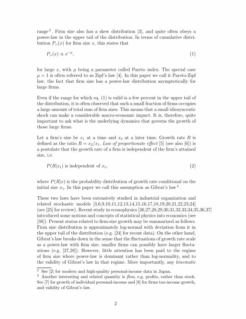
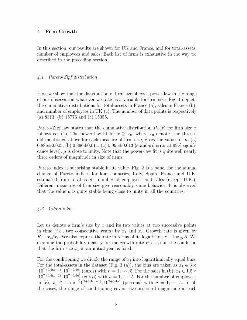
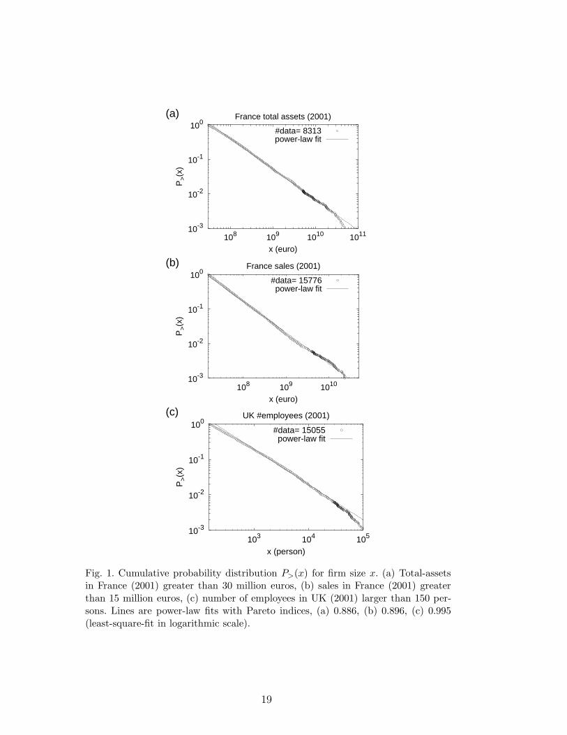
First we show that the distribution of firm size obeys a power-law in the rangeof our observation whatever we take as a variable for firm size. Fig. 1 depictsthe cumulative distributions for total-assets in France (a), sales in France (b),and number of employees in UK (c). The number of data points is respectively(a) 8313, (b) 15776 and (c) 15055.

Pareto-Zipf law states that the cumulative distribution P>(x) for firm size xfollows eq. (1). The power-law fit for x ≥ x0, where x0 denotes the thresh-old mentioned above for each measure of firm size, gives the values of µ; (a)0.886±0.005, (b) 0.896±0.011, (c) 0.995±0.013 (standard error at 99% signifi-cance level). µ is close to unity. Note that the power-law fit is quite well nearlythree orders of magnitude in size of firms.

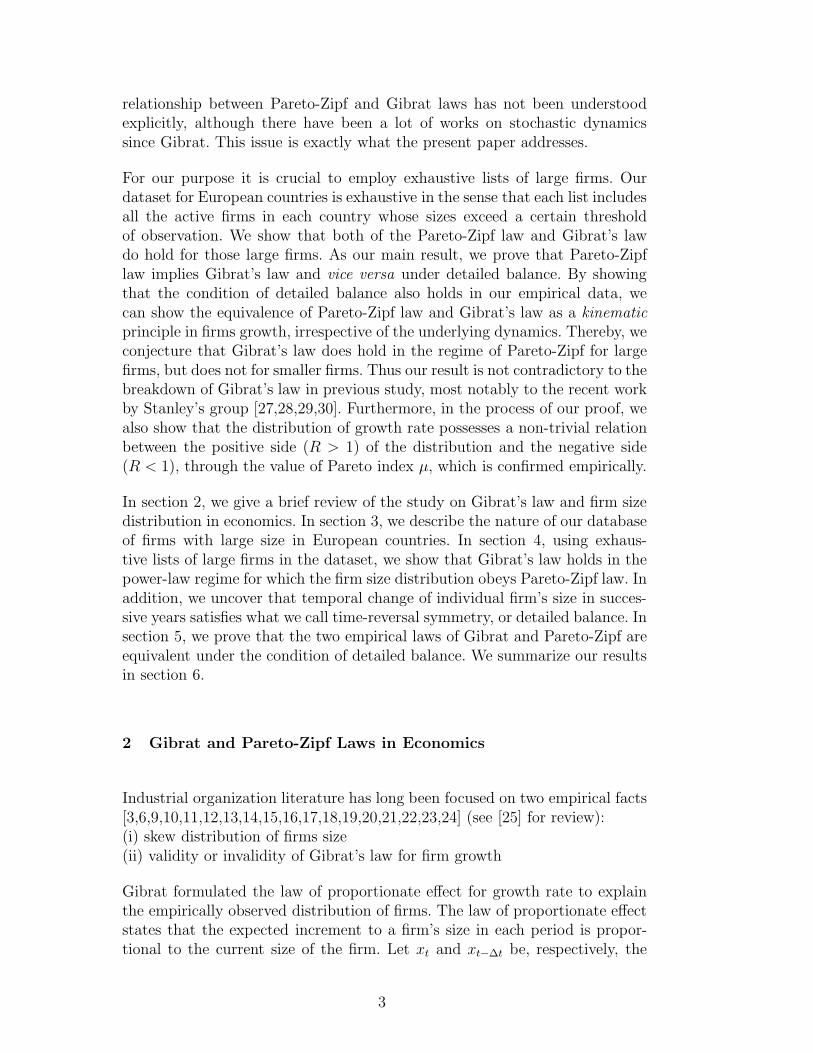
Pareto index is surprising stable in its value. Fig. 2 is a panel for the annualchange of Pareto indices for four countries, Italy, Spain, France and U.K.estimated from total-assets, number of employees and sales (except U.K.).Different measures of firm size give reasonably same behavior. It is observedthat the value µ is quite stable being close to unity in all the countries.

4.2 Gibrat’s law

Let us denote a firm’s size by x and its two values at two successive pointsin time (i.e., two consecutive years) by x1 and x2. Growth rate is given byR ≡ x2/x1. We also express the rate in terms of its logarithm, r ≡ log10 R. Weexamine the probability density for the growth rate P (r|x1) on the conditionthat the firm size x1 in an initial year is fixed.

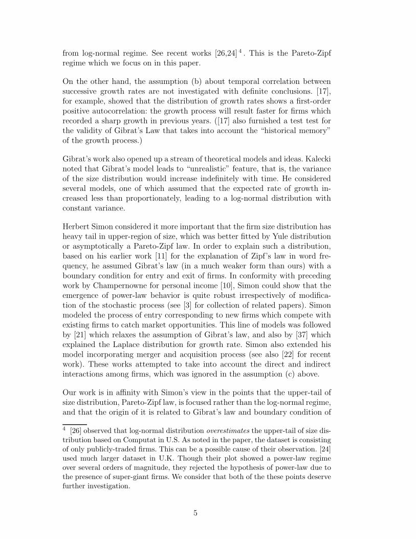
For the conditioning we divide the range of x1 into logarithmically equal bins.For the total-assets in the dataset (Fig. 3 (a)), the bins are taken as x1 ∈ 3×[107+0.4(n−1), 107+0.4n] (euros) with n = 1, · · · , 5. For the sales in (b), x1 ∈ 1.5×[107+0.4(n−1), 107+0.4n] (euros) with n = 1, · · · , 5. For the number of employeesin (c), x1 ∈ 1.5 × [102+0.4(n−1), 102+0.4n] (persons) with n = 1, · · · , 5. In allthe cases, the range of conditioning covers two orders of magnitude in each

8

variable. We calculated the probability density function for r for each bin, andchecked the statistical dependence on x1 by graphical method.

Fig. 3 is the probability density function P (r|x1) for each case. It should benoted that due to the limit x1 > x0 and x2 > x0, the data for large negativegrowth are not available. In all the cases, it is obvious that the function P (r|x1)has little statistical dependence on x1, since all the curves for different ncollapse on a single curve. This means that the growth rate is independent offirm size in the initial year. That is, Gibrat’s law holds.

4.3 Time-reversal symmetry

The validity of Gibrat’s law in the Pareto-Zipf regime appears to be in dis-agreement with recent literature on firm growth. In the next section, we willshow that this is not actually the case by proving that Gibrat and Pareto-Zipf are equivalent under an assumption. The assumption is detailed balance,whose validity is checked here.

Let us denote the joint probability distribution function for the variable x1

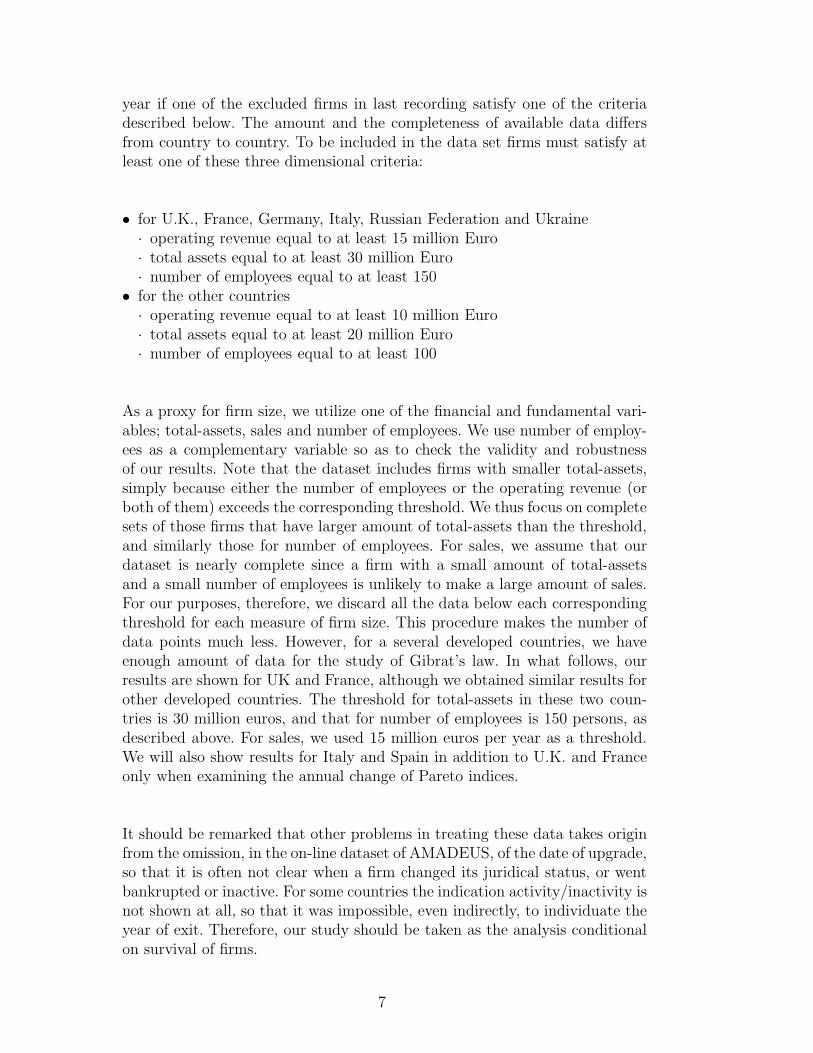
and x2 by P12(x1, x2). The detailed balance, or what we call time-reversal sym-metry, is the assumption that P12(x1, x2) = P12(x2, x1). The joint probabilitiesfor our datasets are depicted in Fig. 4 as scatter-plots of individual firms.

We used two different methods to check the validity of time-reversal symmetry.One is an indirect way to check a non-trivial relationship between the growth-rate in positive side (r > 0) and that in negative (r < 0). That is, as we shallprove in the next section, the probability density distribution in positive andnegative growth rates must satisfy the relation given by eq. (27), if the propertyof time-reversal symmetry holds. We fitted the cumulative distribution only forpositive growth rate by a non-linear function, converted to density function,and predicted the form of distribution for negative growth rate by eq. (27) soas to compare with the actual observation (see Appendix for details). In eachplot of Fig. 3, a solid line in the r > 0 side is such a fit, and a broken line inthe r < 0 side is our prediction. The agreement with the actual observation isquite satisfactory, thereby supporting the validity of time-reversal symmetry.

The other way we took is a direct statistical test for the symmetry in the twoarguments of P12(x1, x2). This can be done by two-dimensional Kolmogorov-Smirnov (K-S) test, which is not widely known but was developed by astro-physicists [43,44,45]. This statistical test is not strictly non-parametric (likethe well-known one-dimensional K-S test), but has little dependence on parentdistribution except through coefficient of correlation. We compare the scatter-plot sample for P12(x1, x2) with another sample for x1 and x2 interchangedby making the null hypothesis that these two samples are taken from a same

9

parent distribution. We used the logarithms ξ1 = log x1 and ξ2 = log x2, andadded constants to ξ1 and ξ2 so that the average growth rate is zero. Thisaddition (or multiplication in x1 and x2) is simply subtracting the nominaleffects due to inflation, etc. We applied two-dimensional K-S test to the re-sulting samples. The null hypothesis is not rejected in 95% significance levelin all the cases we studied.

5 Pareto-Zipf’s law and Gibrat’s law under detailed balance

In the preceding section, we have shown that both of Pareto-Zipf and Gibrat’slaws hold for large firms. This suggests that these two laws are closely relatedwith each other. We show in this section that in fact they are equivalent toeach other under the condition of detailed balance.

Let x be a firm’s size, and let its two values at two successive points in time(i.e., two consecutive years) be denoted by x1 and x2. We denote the jointprobability distribution function (pdf) for the variable x1 and x2 by P12(x1, x2).The joint pdf of x1 and the growth rate R = x2/x1 is denoted by P1R(x1, R).Since P12(x1, x2)dx1dx2 = P1R(x1, R)dx1dR under the change of variables from(x1, x2) to (x1, R), these two pdf’s are related to each other as follows:

P1R

(

x1,x2

x1

)

= x1P12(x1, x2). (3)

We define conditional probabilities:

P1R(x1, R)=P1(x1)Q(R | x1) (4)

=PR(R)S(x1|R), (5)

Both P1(x1) and PR(R) are marginal:

P1(x1) =

∞∫

0

P1R(x1, R)dR

=

∞∫

0

P12(x1, x2)dx2

, (6)

PR(R) =

∞∫

0

P1R(x1, R)dx1, (7)

since the following normalizability conditions are satisfied:

1=

∞∫

0

Q(R|x1)dR, (8)

10

1=

∞∫

0

S(x1|R)dx1. (9)

Three phenomenological properties can be summarized as follows.

(A) Detailed Balance (Time-reversal symmetry):The joint pdf P12(x1, x2) is a symmetric function:

P12(x1, x2) = P12(x2, x1). (10)

(B) Pareto-Zipf’s law:The pdf P1(x) obeys power-law for large x:

P1(x) ∝ x−µ−1, (11)

for x → ∞ with µ > 0.(C) Gibrat’s law:

The conditional probability Q(R | x) is independent of x:

Q(R | x) = Q(R). (12)

We note here that this holds only for large x, because we confirmed itin actual data only in that region, and because otherwise it leads to aninconsistency, as we will see shortly. This relation was called Universalityin [7,8,46,47]. All the arguments below is restricted in this region.

Before starting our discussion of interrelation between these properties, let usfirst rewrite the detailed balance condition (A) in terms of P1R(x1, R):

P1R(x1, R)= x1P12(x1, x2)

= x1P12(x2, x1)

=x1

x2

x2P12(x2, x1)

=R−1P1R

(

x2, R−1)

, (13)

where eq. (10) was used in the second line, and eq. (3) was used in the firstand the third line. The above relation may be rewritten as follows by the useof the conditional probability Q(R | x1) in eq. (5);

Q(R−1 | x2)

Q(R | x1)= R

P1(x1)

P1(x2). (14)

In passing, it should be noted that eq. (13) leads to the following:

11

PR(R)=

∞∫

0

P1R(x1, R)dx1

=

∞∫

0

R−1P1R

(

x2, R−1)

dx1

=

∞∫

0

R−2P1R

(

x2, R−1)

dx2

=R−2PR

(

R−1)

(15)

where eq. (13) was used in the second line, and the third line is merely changeof integration variable. This relation between the marginal growth-rate pdfPR(R) for positive growth (R > 1) and negative growth (R < 1) leads to thefollowing relation, as it should:

∞∫

1

PR(R)dR =

1∫

0

PR(R)dR. (16)

5.1 (A)+(C)→(B)

Let us first prove that the properties (A) and (C) lead to (B). By substitutingthe Gibrat’s law eq. (12) in eq. (14), we find the following:

P1(x1)

P1(x2)=

1

R

Q(R−1)

Q(R). (17)

This relation can be satisfied only by a power-law function eq. (11).

[Proof]Let us rewrite eq. (17) as follows:

P1(x) = G(R)P1(Rx), (18)

where x denotes x1, and G(R) denotes the right-hand side of eq. (17), i.e.

G(R) ≡1

R

Q(R−1)

Q(R). (19)

We expand this equation around R = 1 by denoting R = 1 + ǫ with ǫ ≪ 1 as

P1(x) =G(1 + ǫ)P1((1 + ǫ)x)

12

= (1 +G′(1)ǫ+ · · ·)(P1(x) + P ′

1(x)ǫx + · · ·)

=P1(x) + ǫ(G′(1)P1(x) + xP ′

1(x)) +O(ǫ2), (20)

where we used the fact that G(1) = 1. We also assumed that the derivativesG′(1) and P ′

1(x) exists in the above, whose validity should be checked againstthe results. From the above, we find that the following should be satisfied

G′(1)P1(x) + xP ′

1(x) = 0, (21)

whose solution is given by

P1(x) = Cx−G′(1). (22)

This is the desired result, Pareto-Zipf’s law, and is consistent with the as-sumption made earlier that P ′

1(x) exists. By substituting the result eq. (22)in eq. (19) and eq. (17), we find that

G(R) = RG′(1), (23)

which is consistent with the assumption that G′(1) exists.[Q.E.D.]

From eq. (19) we may calculate G′(1) in terms of derivatives ofQ(R). It should,however, be noted that Q(R) has a cusp at R = 1 as is apparent in Fig. 3,and therefore Q′(R) is expected not to be continuous at R = 1. Bearing thisin mind, we calculate G(1 + ǫ) for 0 < ǫ ≪ 1 as follows:

G(1 + ǫ)≃1

1 + ǫ

Q(1− ǫ)

Q(1 + ǫ)

≃ (1− ǫ)Q(1)− ǫQ−′(1)

Q(1) + ǫQ+′(1)

≃G(1) + ǫ

(

−1 −Q+′(1) +Q−′(1)

Q(1)

)

, (24)

where we denoted the right-derivative and left-derivative of Q(R) at R = 1 bythe signs + and − in the superscript, respectively. From the above, we findthat

G′(1) = −1 −Q+′(1) +Q−′(1)

Q(1), (25)

13

From eq. (22) and eq. (25), we find that

Q+′(1) +Q−′(1)

Q(1)= −µ− 2. (26)

From eqs.(19) and (23), we find the following relation:

Q(R) = R−µ−2Q(R−1), (27)

which should be in contrast to eq. (15). This is related to the point that wementioned in eq. (12): If the Gibrat’s law eq. (12) holds for all x ∈ [0,∞],then PR(R) = Q(R) from eq. (7). If so, eq. (27) contradicts to eq. (15) sinceµ > 0. Besides, the Pareto-Zipf’s law we derived from Gibrat’s law is notnormalizable if it holds for any x. Therefore, Gibrat’s law should hold only forlarge x.

The result eq. (27) shows that the function Q(R) is continuous at R = 1, asis easily seen by substituting R = 1 + ǫ with ǫ > 0 on both hand side andtaking the limit ǫ → +0. Also, by taking the derivative of the both hand sideand taking the limit in a similar manner, we can reproduce eq. (26).

5.2 (A)+(B)→ ?

Let us next examine what we obtain if we had only Pareto-Zipf’s law insteadof Gibrat’s law under the detailed balance.

In this case, substituting the Pareto-Zipf’s law eq. (11) into eq. (14) we findthat

Q(R−1 |Rx)

Q(R | x)= Rµ+2, (28)

where we denote x1 by x and x2 by Rx. We now define a function H(z, x) as

Q(R | x) = xµ+2H(R1/2x, x). (29)

It should be noted that this does not constrain Q(R | x) in any way: arbitraryfunction of the variable R and x can be written in the form of eq. (29). Bysubstituting eq. (29) into eq. (28), we find that

H(R1/2x,Rx) = H(R1/2x, x), (30)

14

which means that the function H(z, x) has the following invariance property.

H(z, x) = H(z, z2/x). (31)

Other than this constraint and some trivial constraint such as continuity, thereis no nontrivial constraint on H(z, x) or Q(R | x).

The results eqs. (29) and (31) is a generalization of the property eq. (27) wefound earlier [7]. In fact, the property eq. (27) follows from eq. (31) in thespecial case:

H(z, x) = Q((z/x)2) x−µ−2, (32)

for which eq. (29) becomes eq. (12), namely the statement of Gibrat’s law.

5.3 (B)+(C)→(A)?

Let us discuss the last question: Under Pareto’s and Gibrat’s laws, what canwe say about the detailed balance? In order to answer this, we use eq. (11)and eq. (12) to write P1R(x,R) for large x as follows:

P1R(x,R) = Ax−µ−1Q(R), (33)

where A is a proportionality constant. According to eq. (13), the detailedbalance is satisfied if this is equal to

R−1P1R(xR,R−1) = Ax−µ−1R−µ−2Q(R−1), (34)

where we used eq. (33). Therefore, we find that the detailed balance conditionis equivalent to eq. (27) in this case.

Summarizing this section, we have proved that under the condition of detailedbalance (A), if the Pareto-Zipf law (B) holds in a region of firm size, then theGibrat’s law (C) must hold in the region, and vice versa. The condition (A)means detailed-balance. On the other hand, if both of (B) and (C) hold, (A)follows provided that eq. (27) holds. eq. (27) is our prediction which gives anon-trivial relation between positive growth (R > 1) and negative (R < 1).This kinematic relation was empirically verified in Fig. 3. See also previouswork [7,8,46,47] for the validity of this relation in personal income and firmstax-income in Japan.

15

6 Summary

The distribution of firm size is quite often dominated by power-law in theupper tail over several orders of magnitude. This regime of Pareto-Zipf lawis different from log-normal distribution in the lower and sometimes widerregime of firm size. The upper tail is occupied by a small number of firms, butthey dominate a large fraction of total sum of firm size.

By using exhaustive datasets of those large firms and with different measuresof firm size in Europe, we show that the Pareto-Zipf law holds as in eq. (1)for firm size x larger than observational threshold x0, and that Gibrat’s law ofproportionate effect holds as in eq. (2) for successive sizes x1 and x2 exceedingx0, stating that the growth rate of each firm is independent of initial size.We also find that detailed balance holds which means that the frequency oftransition from x1 to x2 is statistically the same as that for its reverse process.The Gibrat’s law, Pareto-Zipf’s law and detailed balance condition are relatedto each other. We prove various relationships among them. It follows as one ofthe consequences that there exists a relation between the positive and negativesides of the distribution of growth rate via the Pareto index. The relation isconfirmed empirically in our dataset of European firms.

Acknowledgements

We thank Edmondo Di Giuseppe for helping the preparation of raw datasetsbefore analysis. Y. F. and W. S. thank Katsunori Shimohara for encourage-ment. Supported in part by grants from the Telecommunications AdvancementOrganization in Japan and from Japan Association for Cultural Exchange.

References

[1] V. Pareto, Le Cours d’Economie Politique (Macmillan, London, 1897).

[2] H. Aoyama, W. Souma, Y. Nagahara, M. P. Okazaki, H. Takayasu, M. Takayasu,Fractals 8 (2000) 293.

[3] Y. Ijiri, H.A. Simon, Skew Distributions and the Sizes of Business Firms (North-Holland, New York, 1977).

[4] G. K. Zipf, Human Behavior and the Principle of Least Effort (Addison-Wesley,Cambridge, 1949).

[5] R. Gibrat, Les inegalites economiques (Sirey, Paris, 1932).

16

[6] J. Steindl, Random processes and the growth of firms: A study of the Paretolaw, (Griffin, London, 1965).

[7] Y. Fujiwara, W. Souma, H. Aoyama, T. Kaizoji, M. Aoki, Physica A 321 (2003)598.

[8] H. Aoyama, W. Souma, Y. Fujiwara, Physica A 324 (2003) 352.

[9] M. Kalecki, Econometrica 45 (1945) 161.

[10] D.G. Champernowne, Econometric J. 63 (1953) 318.

[11] H. A. Simon, Biometrika 42 (1955) 425.

[12] P. E. Hart, S. J. Prais, J. Roy. Statist. Soc. A119 (1956) 150.

[13] S. Hymer, P. Pashigian, J. Polit. Econ. 70 (1962) 556.

[14] E. Mansfield, Amer. Econ. Rev. 52 (1962) 1023.

[15] J.M. Samuels, Rev. Econ. Stud. 32 (1965) 105.

[16] A. Singh, G. Whittington, Rev. Econ. Stud. 42 (1975) 15.

[17] A. Chesher, J. Ind. Econ. 27 (1979) 403.

[18] B. H. Hall, J. Ind. Econ. 35 (1987) 583.

[19] D. S. Evans, J. Ind. Econ. 35 (1987) 567.

[20] T. Dunne, M. J. Roberts, L. Samuelson, Rand J. Econ. 19 (1988) 495.

[21] J. Sutton, “The Size Distribution of Businesses, Part I.” STICERD DiscussionPaper No. EI/9, London School of Economics, (1995).

[22] P. McLoughan, Amer. Econ. Rev. 43 (1995) 405.

[23] P. E. Hart, N. Oulton, Econ. J. 106 (1996) 1242.

[24] P. E. Hart, N. Oulton, Applied Econ. Lett. 4 (1997) 205.

[25] J. Sutton, J. Econ. Lit. 35 (1997) 40.

[26] M.H.R. Stanley, S.V. Buldyrev, S. Havlin, R.N. Mantegna, M.A. Salinger,H.E. Stanley, Econ. Lett. 49 (1995) 453.

[27] M.H.R. Stanley, L.A.N. Amaral, S.V. Buldyrev, S. Havlin, H. Leschhorn,P. Maass, M.A. Salinger, H.E. Stanley H.E. Nature 379 (1996) 804.

[28] L.A.N. Amaral, S.V. Buldyrev, S. Havlin, H. Leschhorn, P. Maass,M.A. Salinger, H.E. Stanley, M.H.R. Stanley, J. Phys. (France) I 7 (1997) 621.

[29] S.V. Buldyrev, L.A.N. Amaral, S. Havlin, H. Leschhorn, P. Maass,M.A. Salinger, H.E. Stanley, M.H.R. Stanley, J. Phys. (France) I 7 (1997) 635.

[30] L.A.N. Amaral, S.V. Buldyrev, S. Havlin, M.A. Salinger, H.E. Stanley, Phys.Rev. Lett. 80 (1998) 1385.

17

[31] H. Takayasu, K. Okuyama, Fractals 6 (1998) 67.

[32] K. Okuyama, M. Takayasu, H. Takayasu, Physica A 269 (1999) 125.

[33] J.J. Ramsden, Gy. Kiss-Haypal, Physica A 277 (2000) 220.

[34] R.L. Axtell, Science 293 (2001) 1818.

[35] M. Mizuno, M. Katori, H. Takayasu, M. Takayasu, in Empirical Scienceof Financial Fluctuations: The Advent of Econophysics, H. Takayasu, Ed.(Springer-Verlag, Tokyo, 2002), pp.321–330.

[36] E. Gaffeo, M. Gallegati, A. Palestrini, Physica A 324 (2003) 117.

[37] G. Bottazzi, A. Secchi, Physica A 324 (2003) 213.

[38] H.E. Stanley, L.A.N. Amaral, P. Gopikrishnan, V. Plerou, Physica A 283 (2000)31.

[39] P. Bak, How Nature Works (Copernicus, New York, 1996).

[40] S.F. Nørrelykke, P. Bak, Phys. Rev. E 65 (2002) 036147.

[41] X. Gabaix, “Power laws and the origins of the business cycle”, MIT, Departmentof Economics, preprint (2002).

[42] M. Gallegati, G. Giulioni, N. Kichiji, in Proceedings of 2003 InternationalConference in the Computational Sciences and Its Application, M. L. Gavrilova,V. Kumar, P. L’ecuyer, C. J. K. Tan, Ed.

[43] W. H. Press, S. A. Teukolsky, W. T. Vetterling, B. P. Flannery, NumericalRecipes in C: the art of scientific computing, second edition, (CambridgeUniversity Press, Cambridge, 1992).

[44] J. A. Peacock, Mon. Not. Roy. Astr. Soc. 202 (1983) 615.

[45] G. Fasano, A. Franceschini, Mon. Not. Roy. Astr. Soc. 225 (1987) 155.

[46] Y. Fujiwara, H. Aoyama, W. Souma, in Proceedings of Second Nikkei Symposiumon Econophysics, H. Takayasu, Ed. (Springer-Verlag, Tokyo, 2003), in press.

[47] H. Aoyama, Y. Fujiwara, W. Souma, in Proceedings of Second Nikkei Symposiumon Econophysics, H. Takayasu, Ed. (Springer-Verlag, Tokyo, 2003), in press.

18

10-3

10-2

10-1

100

108 109 1010 1011

P>(x

)

x (euro)

France total assets (2001)

#data= 8313power-law fit

10-3

10-2

10-1

100

108 109 1010

P>(x

)

x (euro)

France sales (2001)

#data= 15776power-law fit

10-3

10-2

10-1

100

103 104 105

P>(x

)

x (person)

UK #employees (2001)

#data= 15055power-law fit

(a)

(b)

(c)

Fig. 1. Cumulative probability distribution P>(x) for firm size x. (a) Total-assetsin France (2001) greater than 30 million euros, (b) sales in France (2001) greaterthan 15 million euros, (c) number of employees in UK (2001) larger than 150 per-sons. Lines are power-law fits with Pareto indices, (a) 0.886, (b) 0.896, (c) 0.995(least-square-fit in logarithmic scale).

19

0

0.5

1

1.5

2

1992 1994 1996 1998 2000 2002

Par

eto

inde

x

year

France

total-assetssales

#employees

0

0.5

1

1.5

2

1992 1994 1996 1998 2000 2002

Par

eto

inde

x

year

Italy

total-assetssales

#employees

0

0.5

1

1.5

2

1992 1994 1996 1998 2000 2002

Par

eto

inde

x

year

Spain

total-assetssales

#employees

0

0.5

1

1.5

2

1992 1994 1996 1998 2000 2002

Par

eto

inde

x

year

UK

total-assets#employees

Fig. 2. Annual change of Pareto indices for Italy, Spain, France and U.K. from 1993to 2001 for total-assets, number of employees, and sales (except U.K.). The estimateof Pareto index in each year was done by extracting a range of distribution corre-sponding to large-size firms, which is common to different countries but different fordifferent measure of size, and by least-square-fit in logarithmic scales of rank andsize.

20

(a)

(b)

(c)

10-2

10-1

100

101

-1 -0.5 0 0.5 1

P(r

|x1)

r

France total assets (2001/2000)

n=12345

10-2

10-1

100

101

-1 -0.5 0 0.5 1

P(r

|x1)

r

France sales (2001/2000)

n=12345

10-2

10-1

100

101

-1 -0.5 0 0.5 1

P(r

|x1)

r

UK #employees (2001/2000)

n=12345

Fig. 3. Probability density P (r|x1) of growth rate r ≡ log10(x2/x1) for the twoyears, 2000/2001. The datasets in (a)–(c) are the same as in eq. (1). Different binsof initial firm size with equal magnitude in logarithmic scale were taken over twoorders of magnitude as described in the main text. The solid line in the portion ofpositive growth (r > 0) is a non-linear fit. The dashed line (r < 0) in the negativeside is calculated from the fit by the relation given in the equation eq. (27).

21

(a)

(b)

(c)

108

109

1010

1011

108 109 1010 1011

x 2 (

euro

)

x1 (euro)

France total assets (2001/2000)

107

108

109

1010

1011

107 108 109 1010 1011

x 2 (

euro

)

x1 (euro)

France sales (2001/2000)

102

103

104

105

102 103 104 105

x 2 (

pers

on)

x1 (person)

UK #employees (2001/2000)

Fig. 4. Scatter-plot of all firms whose size exceeds a threshold. The datasets in(a)–(c) are the same as in eq. (1). Thresholds are (a) 30 million euros for total-assets,(b) 15 million euros for sales, and (c) 150 persons for number of employees. Thenumber of such large firms is respectively (a) 6969, (b) 13099 and (c) 12716.

22

A Fitting distribution of growth rate

For the purpose of fitting probability density function of positive growth rate(R > 1), we used cumulative distribution of positive growth rate, defined by

P+> (R) = Prob{R > R|R > 1}.

P+> (R) can be estimated, as usual, by size versus rank plot restricted only for

R > 1 as follows. Let the number of all firms with R > 1 be N+, and sort theirgrowth rates in descending order: R(1) ≥ R(2) ≥ · · · ≥ R(k) ≥ · · · ≥ R(N+).Then the estimate is given by

P+> (R) =

k

N+= C−1

∫

V (k)

P1R(x1, R)dx1dR,

where V (k) = {(x1, R)|x1 ≥ x0, R ≥ R(k)} (x0 is the observational thresholdmentioned in section 4.1), and C is the normalization:

C =

∞∫

x0

dx1

∞∫

1

dRP1R(x1, R).

Using the observational fact that eq. (12) holds in the region {(x1, R)|x1 ≥x0, R ≥ 1}, the above equation for P+

> (R) reads

P+> (R) = C−1

∞∫

x0

dx1P1(x1)dx1

∞∫

R

dR′Q(R′) = Q0−1

∞∫

R

Q(R′)dR′, (A.1)

where the normalization factor is written by

Q0 =

∞∫

1

Q(R′)dR′. (A.2)

By taking derivative of eq. (A.1) with respect to R, it follows that

Q(R) = −Q0d

dRP+> (R). (A.3)

We empirically found that the rank-size plot can be well fitted by a non-linearfunction of the form:

log10 P+> (R = 10r) = −a(1 − e−br)− cr ≡ F (r), (A.4)

23

10-3

10-2

10-1

100

0 0.2 0.4 0.6 0.8 1

P>+(r

|x1)

r

France total assets (2001/2000)

n=12345

allfit

Fig. A.1. Cumulative probability P+> (R = 10r) for the growth of total-assets in

France (2001/2000). n is the index of bin used in Fig. 3 (a), “all” means the plotfor all the dataset of positive r. “Fit” is done by the non-linear function given bythe equation eq. (A.4).

where a, b and c are parameters. An example is given in Fig. A.1 for Francetotal-assets (2001/2000). Cumulative probabilities P+

> (r|x1) (the left-handside of eq. (A.4)) conditioned on an initial year’s total-assets are shown foreach of the same bins used in Fig. 3 (a), but restricted to the data with posi-tive r. The non-linear fit done by eq. (A.4) is represented by a solid and boldline in the figure. Note also that the curves for different bins almost collapsebecause of the statistical independence of x1.

Under the change of variable, r = log10 R, the probability density for r definedby q(r) is related to that for R by

log10 q(r) = log10Q(R = 10r) + r + log10(ln 10) (A.5)

Therefore it follows from eq. (A.3) and eq. (A.5) that

log10 q(r) = F (r) + log10

[

−dF (r)

dr

]

+ log10Q0 + log10(ln 10). (A.6)

In each plot of Fig. 3, the solid curve is given by eq. (A.6), where P (r|x1)denotes the probability density function q(r) for r, conditioned on an initialyear’s size x1.

The relation eq. (27) for positive (R > 1) and negative (R < 1) growth ratescan be written in terms of q(r) as

log10 q(r) = −µr + log10 q(−r), (A.7)

24

which is easily shown by eq. (A.5). In each plot of Fig. 3, the dotted curve fornegative growth rate (r < 0) is obtained from the solid curve for positive one(r > 0) through the relation eq. (A.7).

25