An analytical Jacobian approach to sparse reaction

kinetics for computationally efficient combustion

modelling with large reaction mechanisms

Federico Perini,∗,†,‡ Emanuele Galligani,¶ and Rolf D. Reitz‡

Dipartimento di Ingegneria Meccanica e Civile, Università di Modena e Reggio Emilia, I-41125

Modena, Italy, Engine Research Center, University of Wisconsin–Madison, Madison 53703, USA,

and Dipartimento di Matematica pura ed applicata “G. Vitali”, Università di Modena e Reggio

Emilia, I-41125 Modena, Italy

E-mail: federico.perini@unimore.it

Abstract

This study presents an analytical Jacobian formulation for detailed gas-phase reaction ki-

netics, suitable for accurate and computationally efficient combustion simulations using either

skeletal or detailed reaction mechanisms. A general chemical kinetics initial value problem

in constant volume environments is considered, where the gas-phase mixture thermodynamic

properties are polynomial functions of temperature according to the JANAF standard. Three

different reaction behaviours are accounted for, including modified Arrhenius kinetic law re-

actions, third-body collisions, and pressure dependent reactions in Lindemann’s or Troe’s ki-

netic law forms. The integration of the chemistry ODE system is carried out using a software

package specifically developed in Fortran language, and the solution compared to a reference

∗To whom correspondence should be addressed†University of Modena‡University of Wisconsin–Madison¶University of Modena

1

chemical kinetics library. Two analytical Jacobian formulations, an exact one and a sparser,

approximate one are proposed, and compared to numerical Jacobians computed by finite differ-

ences internally generated by a variety of commonly used stiff ordinary differential equations

(ODE) solvers. The results show significant reductions in total computational times for the

chemistry ranging from factors of 2 to more than two orders of magnitude for 29 species, 56

reactions to 2878 species, 8555 reactions, respectively. Finally, the code has been coupled to

an engine combustion simulation software, where at each timestep the chemistry ODE system

is integrated in each cell of the computational grid, allowing 77% faster computations with a

160 species combustion mechanism.

Introduction

Recent developments in combustion research show that there is urgent need for incorporating de-

tailed reaction mechanisms in multidimensional simulations.1 The development of comprehensive

reaction mechanisms, consisting of thousands reactions and species, for the oxidation of a variety

of fuels has been growing in the past two decades, and has allowed significant insight in many

combustion phenomena to be achieved.2,3 As a matter of fact, most recently developed reaction

mechanisms range from about 1000 to more than 3000 species, up to more than 10000 elemen-

tary reactions;4–7 the computational requirements of simulations involving such large mechanisms

are huge even for simple batch reactor simulations, or one dimensional steady laminar flame cal-

culations,8 thus making their adoption practically unviable – even on distributed computational

clusters – for most practical combustion systems of industrial interest, whose computational do-

mains typically require from a few thousands to several million cells.1 A paradigmatic example

is that of internal combustion engine research, where since the early 2000’s the introduction of

necessarily skeletal or reduced chemistry computations in engine computer modelling has never-

theless allowed the study and the development of new, kinetically- or reactivity-driven combustion

concepts such as the homogeneous-charge compression ignition (HCCI) and reactivity-controlled

compression ignition (RCCI).9–12

2

For these reasons, a number of techniques have been developed in order to reduce the computa-

tional efforts needed by the integration of the chemistry system of ordinary differential equations

(ODE). Among them, most approaches target the reaction mechanism, aiming at locally reduc-

ing its size, complexity or stiffness, while keeping the introduced error under control.13–19 The

present work belongs instead to a smaller class of methods devoted to tailoring the problem for-

mulation and the integration methodology to the solution of the reaction kinetics problem. When

dealing with combustion computations, the solution of the stiff ODE system associated with chem-

ical kinetics usually relies on robust solvers using backward differentiation formulae methodsa

(BDF);20–25 those methods however pursue Newton iterations which require repeated Jacobian

matrix evaluations. In order to cope with the increasing demand of this operation with the in-

crease in mechanism size, some Jacobian approaches to chemical kinetics simulations have been

developed, aiming at either approximating26,27 or preconditioning28–30 the ODE system’s Jacobian

matrix. The system Jacobian matrix is usually approximated via finite differences, while the di-

rect, analytical formulation is only common in kinetics problems which do not undergo strong

temperature-kinetics coupling.31–33 For practical combustion simulations, instead, mechanism-

specific routines can be built by adopting symbolic analysis tools for pre-processing,34–36 so that

the computation is mechanism-specific, and does not allow insight to be gained for improving the

overall computational efficiency. These methods typically do not allow the Jacobian matrix to

be built adopting sparse matrix algebra,37,38 which can enable significant computational savings

when coupled to sparse ODE solvers.39,40 Nevertheless, some strategies can be adopted, such as

to reduce the number of calls to the ODE system function for evaluating the finite-difference Jaco-

bian when a sparsity pattern is provided.41 The DAEPACK automatic differentiation library42,43

can provide a sparse representation of the Jacobian matrix using proprietary subroutines, as for

example applied by Schwer et al.44 to combustion chemistry cases. The library generates routines

for evaluating the Jacobian that assemble the single partial derivatives computations into a sparse

aBackward differentiation formulae were first proposed by Curtiss and Hirschfelder20 up to orders 1 and 2, and byGear21 up to order 6. The ‘stiff’ term referred to ordinary differential equations systems has in fact been introduced byCurtiss and Hirschfelder.20 The first BDF implementation, with variable order and step, is Gear’s well known DIFSUBroutine (Gear,21 Section 9.3).

3

matrix representation. Such approaches however perform item-by-item operations to compute

the partial derivatives, and cannot build the final sparse matrix by just exploiting essential sparse

matrix-vector and matrix-matrix operations. Also, the forward mode of automatic differentiation

procedure is acknowledged to compute the Jacobian in a non-minimum number of operations42

that can make the overall evaluation computationally expensive when dealing with large systems.

Finally, explicit and matrix-free integration methods are recently gaining interest for their ability

to pursue the integration of the stiff ODE system without requiring expensive solutions of linear

systems of equations (see, for example, the works by Mosbach and Kraft45 and Lee and Gear46).

However, implicit methods provide better performance for the accuracy required for practical stiff

combustion calculations.45 A sparse, universal analytical Jacobian evaluation thus appears to be

suitable to address the following important issues arising when integrating chemical kinetics for

practical combustion problems:

• Scaling of the computational demand for the system’s Jacobian matrix of arbitrary homo-

geneous gas-phase reactors (of the order of n2s when evaluated through finite differences, ns

being the number of gas-phase species);

• Dense matrix storage requirements (also of the order of n2s );

• Scaling of the computational costs for matrix factorization (of the order of n3s if dense matrix

algebra is employed);

• Exploitation of mechanism sparsity, which is significant even for small (ns < 50) reaction

mechanisms.

We thus focus on the development of an exact, analytical Jacobian formulation for arbitrary

detailed chemical kinetics initial value problems, considering different reaction behaviours, and

including accurate prediction of gas-phase mixture thermodynamic properties according to the

JANAF 7-coefficient polynomial standard.47 The aim is to reduce the cost of simulations with ar-

bitrary reaction mechanisms, and to achieve an efficient scaling of the computational demand with

4

increasing number of species and reactions. We show that the proposed approach is able to speed

up reference calculations from about two times for small, almost dense reaction mechanisms, and

up to more than two orders of magnitude for large comprehensive mechanisms.

This paper is organised as follows. In the first paragraph the approach adopted for the evalu-

ation of chemical kinetics in constant-volume adiabatic environments is presented. Then, in the

second section the entries of the whole ODE system’s sparse Jacobian matrix are derived, in both

a complete, exact formulation and under an approximating assumption which enhances the ma-

trix sparsity. Finally, a fast polynomial approach to the evaluation of the complex temperature-

dependent functions is presented in the last section.

The validation and the analysis of the proposed analytical Jacobian approach in terms of compu-

tational efficiency is presented in the Results section, where an extensive validation testbench has

been set up considering three reaction mechanisms of different sizes, ranging from 29 species and

52 reactions to 2878 species and 8555 reactions. 18 reactor configurations are considered for each

combustion mechanism, spanning broad ranges of initial reactor pressure, temperature and mix-

ture composition, in order to maximise the variety of stiffness conditions that may occur during

the integration of the chemistry ODE system, together with five well established stiff ODE solvers.

Finally, the results of the code’s performance when coupled to a widely adopted computational

fluid dynamics (CFD) code for internal combustion engine simulations are presented. The Appen-

dices report essential details of the approach, including the partial derivatives, and full initialisation

details for the test cases.

Description of the chemical kinetics problem

In the present study the chemical kinetics of reactive gaseous mixtures are evaluated using a mod-

ular code written in Fortran, which is used both for computing gaseous mixture thermodynam-

ics and finite reaction kinetics.48 The initial value problem considers time evolution of an adia-

5

batic, constant-volume, homogeneous gas-phase chemically reacting environment, whose solution

is given throughout the integration of a system of ordinary differential equations. The independent

variables are the species mass fractions, and the average system temperature.49

Mass conservation

The reaction mechanism is represented by a set of nr reactions involving a total number ns of

chemical species. Each k-th reaction is expressed as:

ns

∑i=1

ν′k,iMi

ns

∑i=1

ν′′k,iMi, k = 1, · · · ,nr, (1)

where the stoichiometric coefficients are stored as sparse matrices ν ′ and ν ′′ of nr rows and ns

columns, and M identifies the names of the chemical species in the mechanism. This general

reaction kinetics framework leads to a set of ns ODEs expressing mass conservation for the system:

dYi

dt=

Wi

ρ

nr

∑k=1

(ν′′k,i−ν

′k,i)

qk(Y ,T ), i = 1, · · · ,ns, (2)

where Wi is the species molecular weight and ρ > 0 the average system density. The reaction

rates of progress variables, qk, are generally dependent on temperature T and on the species mass

fractions of the involved species. Their behaviour can indeed have different forms depending on

their specific interactions. Four different reaction formulations have been considered, for which

specific analytical derivatives have then been obtained. Below, we give full details about these

formulations, as they are needed in the following for building the analytical Jacobian matrix. First

of all, simple reactions follow the plain law of mass action:

qk(Y ,T ) = κ f ,k

ns

∏i=1

(ρYi

Wi

)ν ′k,i−κb,k

ns

∏i=1

(ρYi

Wi

)ν ′′k,i(3)

= q f ,k(Y ,T )−qb,k(Y ,T ),

6

where the forward and backward reaction rate constants are temperature-dependent, and follow the

modified Arrhenius kinetic law:

κ f ,k (T ) = Ak T bk exp(− Ek

RT

). (4)

Backward reaction rates, in particular, can be expressed similarly to forward reaction rates, but are

usually derived from the equilibrium constant:

κb,k (T ) = κ f ,k (T )/Kceq,k (T ) , (5)

Kceq,k (T ) = exp(−∆g0

k) ( patm

RT

)∑

nsi=1 (ν ′′k,i−ν ′k,i)

,

where ∆g0k = ∑i=1,ns

(ν ′′k,i−ν ′k,i

)g0

i is the reaction’s change in non-dimensional Gibbs free energy,

g0i = H0

i /(RT )− S0i /R, between reactants and products. In case a non reversible reaction occurs,

simply κb,k = 0.

In third-body reactions (TB), the presence in the mixture of other molecules than those participat-

ing in the reaction itself enhances the reaction speed proportionally to an ‘effective’ concentration,

or molecularity, Me f f :

qT Bk (Y ,T ) = Me f f ,k(Y ,T )qk(Y ,T ), (6)

Me f f ,k(Y ,T ) =ns

∑i=1

(αi,k

ρ Yi

Wi

)=Ctot−

ns

∑i=1

(βi,k

ρ Yi

Wi

),

where in the simplest case each species equally participates to the reaction improvement (i.e.

αi, j = 1 or βi, j = 1−αi, j = 0), but enhanced reaction molecularity coefficients can be defined

for some species.

The effective molecularity value is a parameter also in pressure-dependent reactions, where a sim-

ple reaction rate, as from Eq. 4, does not suit the reaction behaviour at different pressure values.

In this case, two modified Arrhenius formulations describe the high- and low-pressure limits for

the forward reaction rates, namely κ f ,0 and κ f ,∞. The effective reaction rate at a defined pressure

7

value is hence determined by a weighting factor to the high-pressure limit rate:

κPDf ,k = κ f ,k,∞ FPD

k . (7)

In simple pressure-dependent reactions, which follow Lindemann’s kinetic law form (PD,Lind),

the weighting factor for pressure dependence is a function of the reduced pressure value, Pr =

κ f ,0 Me f f /κ f ,∞ which defines the actual reaction rate by averaging between the two limits. In

Troe’s kinetic law formulation (PD,Troe), instead, a more complex pressure factor multiplies κ f ,∞,

whose detailed description and derivation is given in the Appendix.

FPD,Lindk = Prk/(1+Prk) = Pcor,k, (8)

FPD,Troek = Prk/(1+Prk) ·10logFTroe

k = Pcor,k ·10logFTroek .

Due to the thermodynamic constraints between forward and backward reaction rates, the overall

rate of progress variable for pressure dependent reactions can hence be written as:

qPDk (Y ,T ) = FPD

k (Y ,T )qk(Y ,T ), (9)

where the regular expression qk is computed using the high-pressure limit rate κ f ,k,∞ in Equation

3.

Closure equation

The initial value problem (IVP) for the chemically reacting environment needs closure through

the energy conservation equation. In this work, the perfectly adiabatic constant-volume reactor

is considered, as this condition is the one usually occurring when incorporating the solution of

detailed chemistry into multidimensional CFD codes, where the species and internal energy source

terms for each cell are computed as part of a subcycling strategy for the whole code. In particular,

the internal energy source term gives a change in the average reactor temperature:

8

dTdt

(Y ,T ) =− 1cv (Y ,T )

ns

∑i=1

(Ui (T )

Wi

dYi

dt(Y ,T )

), (10)

where cv = ∑i=1,ns (YiCv,i/Wi) is the mass average mixture specific heat at constant volume, and Ui

the molar internal energy values of the speciesb.

Equations 2 and 10 thus constitute the autonomous IVP in neq = ns +1 problem unknowns, repre-

sented by the array y = [T,Y1, · · · ,Yns]T :

y′ = f (y) =

dT/dt

dY1/dt

· · ·

dYns/dt

, y(t = 0) = y0. (11)

Jacobian formulation

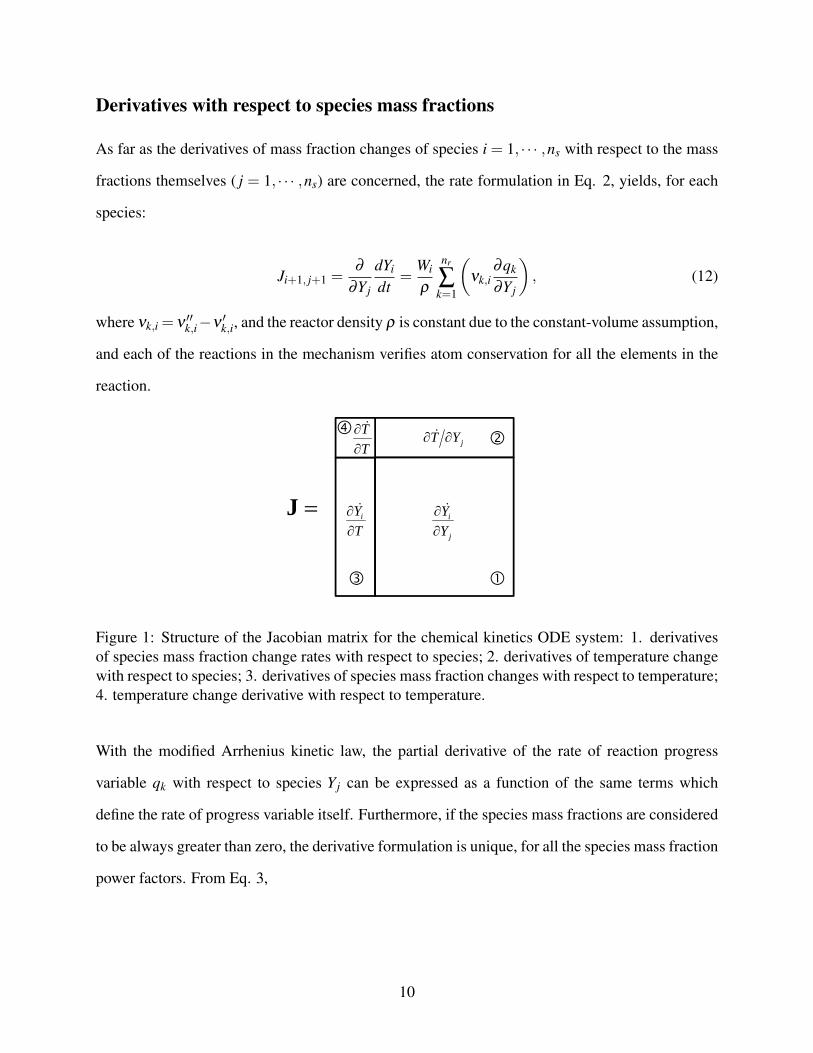
The Jacobian matrix J = ∂ fi/∂y j has a sparse bordered structure as highlighted in Figure 1: the

first element – i.e. the entry in position (1,1) –, the rest of the first row and of the first column

are dense, and contain the derivatives of the temperature and species mass fraction rates of change

with respect to temperature, and the derivatives of the temperature rate of change with respect to

species mass fractions, respectively. The remaining square part of the Jacobian matrix is instead

sparse, and contains the derivatives of the species mass fraction time derivatives with respect to the

species mass fractions. As a matter of fact, the sparsity in the Jacobian formulation descends from

the sparsity of matrices ν ′ and ν ′′, where, considering elementary reactions, usually not more than

three different reactants and three different products coexist.

bThermodynamic properties: we use lower-case characters for mass specific quantities, and uppercase charactersfor molar quantities. Bar expresses mixture average properties, bold indicates column vector or 2-d matrix.

9

Derivatives with respect to species mass fractions

As far as the derivatives of mass fraction changes of species i = 1, · · · ,ns with respect to the mass

fractions themselves ( j = 1, · · · ,ns) are concerned, the rate formulation in Eq. 2, yields, for each

species:

Ji+1, j+1 =∂

∂Y j

dYi

dt=

Wi

ρ

nr

∑k=1

(νk,i

∂qk

∂Yj

), (12)

where νk,i = ν ′′k,i−ν ′k,i, and the reactor density ρ is constant due to the constant-volume assumption,

and each of the reactions in the mechanism verifies atom conservation for all the elements in the

reaction.

J

jYT T

T

J

j

i

Y

Y

T

Yi

Figure 1: Structure of the Jacobian matrix for the chemical kinetics ODE system: 1. derivativesof species mass fraction change rates with respect to species; 2. derivatives of temperature changewith respect to species; 3. derivatives of species mass fraction changes with respect to temperature;4. temperature change derivative with respect to temperature.

With the modified Arrhenius kinetic law, the partial derivative of the rate of reaction progress

variable qk with respect to species Yj can be expressed as a function of the same terms which

define the rate of progress variable itself. Furthermore, if the species mass fractions are considered

to be always greater than zero, the derivative formulation is unique, for all the species mass fraction

power factors. From Eq. 3,

10

∂qk

∂Yj=

1Yj

[ν′k, jκ f ,k

ns

∏r=1

(ρYr

Wr

)ν ′k,r−ν

′′k, jκb,k

ns

∏s=1

(ρYs

Ws

)ν ′′k,s]

(13)

=1Yj

[ν′k, j q f ,k−ν

′′k, j qb,k

], ∀Yj > 0, j = 1, · · · ,ns

and thus only the terms where either ν ′k, j 6= 0 or ν ′′k, j 6= 0 exist. This formulation is complete

for modified Arrhenius kinetic law reactions only, but is computed for all the reactions in the

mechanism, since more complex formulations can be written as developments of this simple form.

In particular, for more complex reaction behaviours such as third-body reactions, the expression of

the effective molecularity is common to all of them. From Equation 6,

∂qT Bk

∂Yj=

∂Me f f ,k

∂Yjqk +Me f f ,k

∂qk

∂Yj. (14)

In order to cope with the effects of the derivative of the effective molecularity term, which

linearly depends on each species mass fraction, thus leading to dense lines in the Jacobian matrix

for each species participating in third-body reactions, an alternative formulation has been tested,

and its form is discussed in detail in the next section.

Pressure dependent reactions behave similarly to third-body reactions, but the multiplying factor to

the baseline rate of progress variable is now a function of effective molecularity and of both high-

and low-pressure limit rate formulations. From Equation 9:

∂qPDk

∂Yj=

∂FPDk

∂Yjqk +FPD

k∂qk

∂Yj. (15)

11

Reactions which follow Lindemann’s kinetic law have:

∂FPD,Lindk∂Yj

=∂Pcor,k

∂Yj(16)

=∂Me f f ,k

∂Yj

κ f ,k,0 κ f ,k,∞(κ f ,k,0 Me f f ,k +κ f ,k,∞

)2 ,

while reactions under Troe’s kinetic law form have:

∂FPD,Troek∂Yj

= 10logFTroek

[∂Pcor,k

∂Yj+ log(10)Pcor,k

∂ logFTroek

∂ logPrk

∂ logPrk

∂Yj

]. (17)

The dependence of the base-10 logarithm of Troe’s centering factor with respect to the logarithm

of the reduced pressure value is extensive, and is discussed in the Appendix.

The computation of the sparse central part of the Jacobian matrix (zone 1, Figure 1), also gives the

bricks for building the Jacobian’s upper border, i.e., the derivatives of temperature variation with

respect to species mass fractions. From Eq. 10, the components of block J­ are:

J1, j+1 =∂

∂Yj

(dTdt

)=− 1

cv

[Cv, j

Wj

dTdt

+ns

∑i=1

Ui

Wi

∂

∂Yj

(dYi

dt

)], (18)

it can be noted that the column vector containing all of the derivatives of temperature change with

respect to species can be evaluated as the product

JT­ =

(∂

∂Y1

(dTdt

), · · · , ∂

∂Yns

(dTdt

))T

(19)

=∂

∂Y

(dTdt

)=− 1

cv

(cv

dTdt

+ JT¬ u),

where lower-case cv, j and u j indicate specific quantities in mass units, and the square block J¬ is

usually very sparse.

12

Derivatives with respect to temperature

In order to build the first column of the Jacobian matrix, derivatives of the species thermody-

namic properties need to be evaluated. In the present approach, the 7-coefficient JANAF standard

approach47 is considered. The detailed polynomial expressions of the derivatives involving the

species constant-volume molar specific heat, ∂Cv, j/∂T , Gibbs free energy ∂g0j/∂T are reported

in the Appendices. Two sets of polynomial coefficients are usually provided for each species, for

better fitting of the low- and of the high-temperature ranges. The behaviour of the resulting func-

tions is however of class C2 in the whole temperature domain, including the switching temperature

value. Hence, it is guaranteed that the analytically differentiated functions can apply the same sets

of coefficients as the parent functions, and over the same temperature validity ranges.

Concerning the derivatives of species mass fraction rates with respect to temperature, they

descend from the temperature derivatives of the reaction rates of the progress variable they are

involved in:

J j+1,1 =∂

∂T

(dYj

dt

)=

Wi

ρ

nr

∑k=1

νk, j∂qk

∂T, (20)

where, again, the reaction-dependent derivatives ∂qk/∂T have a base expression for the modi-

fied Arrhenius kinetic law reactions, which can be evolved to consider third-body and pressure-

dependent reaction behaviours. The modified Arrhenius formulation considers reaction rates in

the form of Eq. 4, thus

∂κ f ,k

∂T=

κ f ,k

T

(bk +

Ek

RT

). (21)

Backward reaction rates derivatives follow the same formulation if they are explicitly expressed

in modified Arrhenius form, while, in the case where they are computed from the equilibrium

constant,

∂κb,k

∂T=

1Kceq,k

(∂κ f ,k

∂T− 1

Kceq,k

∂Kceq,k

∂Tκ f ,k

), (22)

13

where the derivative of the equilibrium constant of reaction k in concentration units only depends

on temperature:

∂Kceq,k

∂T=−Kceq,k

∑nsj=1

(ν ′′k, j−ν ′k, j

)T

+∂(∆g0

k

)∂T

. (23)

As forward and backward reaction rates are the only temperature-dependent parameters in

the rate of progress variable formulation, for constant-volume reactors where the average mixture

density is constant, the rate of progress variable derivative yields:

∂qk

∂T=

∂κ f ,k

∂T

ns

∏r=1

(ρ Yr

Wr

)ν ′k,r−

∂κb,k

∂T

ns

∏s=1

(ρ Ys

Ws

)ν ′′k,s. (24)

If a third-body reaction is considered, the rate of progress variable is obtained simply multiply-

ing its baseline formulation by an effective molecularity value, thus

∂qT Bk

∂T=

∂qk

∂TMe f f ,k, (25)

as in constant-volume problems the effective molecularity value of Eq. 6 does not show any de-

pendence on temperature. This is not true in presence of pressure-dependent reactions, where

the enhancement factor which multiplies the ‘standard’ rate of progress variable formulation is a

function of the average pressure value, and is thus tightly bound to temperature:

∂qPDk

∂T= qk

∂FPDk

∂T+FPD

k∂qk

∂T; (26)

∂FPD,Lindk∂T

=Me f f ,k(

κ f ,k,∞ +κ f ,k,0Me f f ,k)2

(κ f ,k,∞

∂κ f ,k,0

∂T−κ f ,k,0

∂κ f ,k,∞

∂T

);

∂FPD,Troek∂T

= 10logFTroek

(∂FPD,Lind

k∂T

+ log(10)∂ logFTroe

k∂T

).

Once the species derivatives with respect to temperature have been assembled considering the

14

proper reactions contributions, the first item in the Jacobian matrix can be computed, yielding the

derivative of the average mixture temperature change rate with respect to the system temperature

itself:

∂

∂T

(dTdt

)=− 1

cv

{dTdt

∂cv

∂T+

ns

∑i=1

[1

Wi

(Cv,i

dYi

dt+Ui Ji+1,1

)]}. (27)

Jacobian sparsity pattern

As previously mentioned, the standard expression of the effective molecularity for third-body and

pressure dependent reactions involves all the species in the mechanism, and the molecularity coef-

ficients α j,k of Eq. 6 are normally unity, except in the case where the molecular structure of some

species can improve the efficiency of inter-molecular collisions in the reactions more than the oth-

ers. Since the presence of enhanced third-body molecularity coefficients is usually limited to a

restricted number of species - not more than five or six species per third-body reaction -, Schwer et

al.44 proposed a more efficient storage of the molecularity coefficient: β j,k = 1−α j,k. In this case,

only the non-zero entries of β j,k, corresponding to the species which show an enhancing behaviour

towards modifying the average collision frequency need to be stored and used for computing the

effective molecularity value:

Me f f ,k =Ctot−ns

∑i=1

βi,k

(ρ Yi,k

Wi

)= ρ

ns

∑i=1

Yi

Wi−

ns

∑i=1

βi,k

(ρ Yi,k

Wi

)(28)

As Equation 28 shows, the derivatives of the effective reaction molecularity Me f f ,k with respect

to each of the species mass fractions are always non-zero in constant-volume environments, where

the total mixture concentration Ctot , in mole units, is not conserved during the time evolution of

the adiabatic reactor:

∂Ctot

∂Yj=

ρ

Wj=

1RT

∂ p∂Yj

. (29)

Since this condition would not be present in adiabatic constant pressure environments, where

15

the average mixture concentration in mole units is constant, we have introduced the approximate,

yet sparser Jacobian formulation, which assumes that ∂Ctot/∂Y j ≈ 0, ∀ j = 1, · · · ,ns. This formula-

tion does not affect the ODE system evaluation, but only the Jacobian estimation. The rows related

to the species which take part into third-body reactions are almost completely cleared, and only

the columns containing derivatives with respect to species with enhanced molecularity coefficients

remain non-zero. The main aim of this approximate approach is to maximize the computational

efficiency of the analytical Jacobian computation, through setting up a much sparser matrix layout.

The error introduced by the approximation is expected not to affect too much the integration re-

sults when using common stiff ODE solvers, which usually perform simplified Newton iterations

through computing the Jacobian only once and then using the saved version at each Newton step

(see the VODE integrator,22 for example).

In Table 1, the features of three widely used reaction mechanisms, related to the oxidation of

n-heptane and methyl-decanoate, common surrogate species which well suit the ignition charac-

teristics of diesel and biodiesel fuels, are presented. The mechanism dimensions range from 29

species to 2878 species, the first one well representing a class of skeletal mechanisms commonly

adopted in multidimensional CFD codes; the latter being among the widest detailed mechanisms

available in the literature involving fuel compounds.1 A graphical representation of the Jacobian

matrix sparsity in the three cases, comparing the complete and the sparser approximate formula-

tions, is shown in Figure 2. Note that the sparsity increases fast for the semi-detailed n-heptane

mechanism, where even using the ‘complete’ third-body formulation, the matrix sparsity reaches

72%. Extreme matrix sparsity is observed in the largest mechanism, where only 0.6% of the ele-

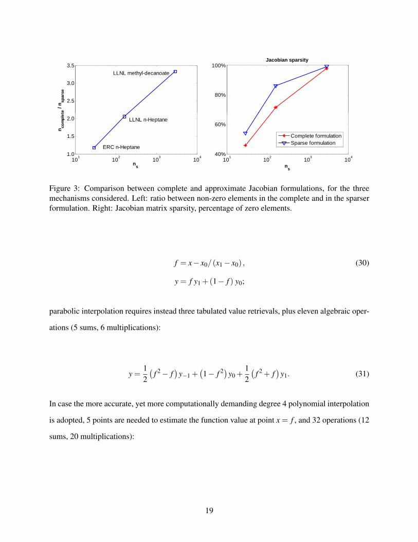
ments is non-zero in the sparse third-body formulation. Figure 3 shows the relationship between

matrix sparsity and mechanism dimension, where a quasi-logarithmical sparsity trend is observed

for the Jacobian using the complete third-body formulation, while a lower sparsity increase rate

characterizes the sparse formulation, where the number of third-body reactions in the mechanism

also becomes an important factor affecting Jacobian sparsity.

16

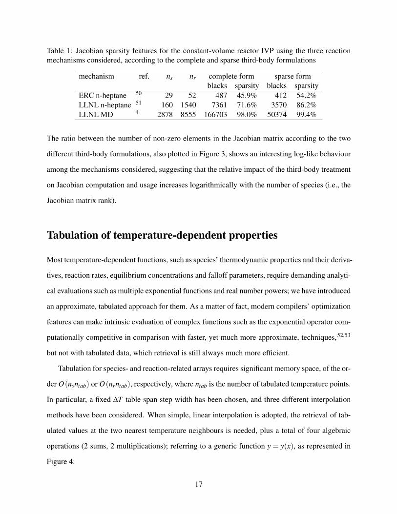
Table 1: Jacobian sparsity features for the constant-volume reactor IVP using the three reactionmechanisms considered, according to the complete and sparse third-body formulations

mechanism ref. ns nr complete form sparse formblacks sparsity blacks sparsity

ERC n-heptane 50 29 52 487 45.9% 412 54.2%LLNL n-heptane 51 160 1540 7361 71.6% 3570 86.2%LLNL MD 4 2878 8555 166703 98.0% 50374 99.4%

The ratio between the number of non-zero elements in the Jacobian matrix according to the two

different third-body formulations, also plotted in Figure 3, shows an interesting log-like behaviour

among the mechanisms considered, suggesting that the relative impact of the third-body treatment

on Jacobian computation and usage increases logarithmically with the number of species (i.e., the

Jacobian matrix rank).

Tabulation of temperature-dependent properties

Most temperature-dependent functions, such as species’ thermodynamic properties and their deriva-

tives, reaction rates, equilibrium concentrations and falloff parameters, require demanding analyti-

cal evaluations such as multiple exponential functions and real number powers; we have introduced

an approximate, tabulated approach for them. As a matter of fact, modern compilers’ optimization

features can make intrinsic evaluation of complex functions such as the exponential operator com-

putationally competitive in comparison with faster, yet much more approximate, techniques,52,53

but not with tabulated data, which retrieval is still always much more efficient.

Tabulation for species- and reaction-related arrays requires significant memory space, of the or-

der O(nsntab) or O(nrntab), respectively, where ntab is the number of tabulated temperature points.

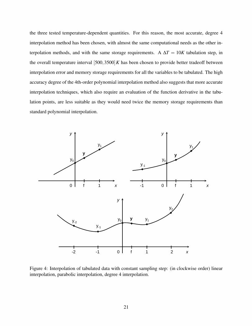
In particular, a fixed ∆T table span step width has been chosen, and three different interpolation

methods have been considered. When simple, linear interpolation is adopted, the retrieval of tab-

ulated values at the two nearest temperature neighbours is needed, plus a total of four algebraic

operations (2 sums, 2 multiplications); referring to a generic function y = y(x), as represented in

Figure 4:

17

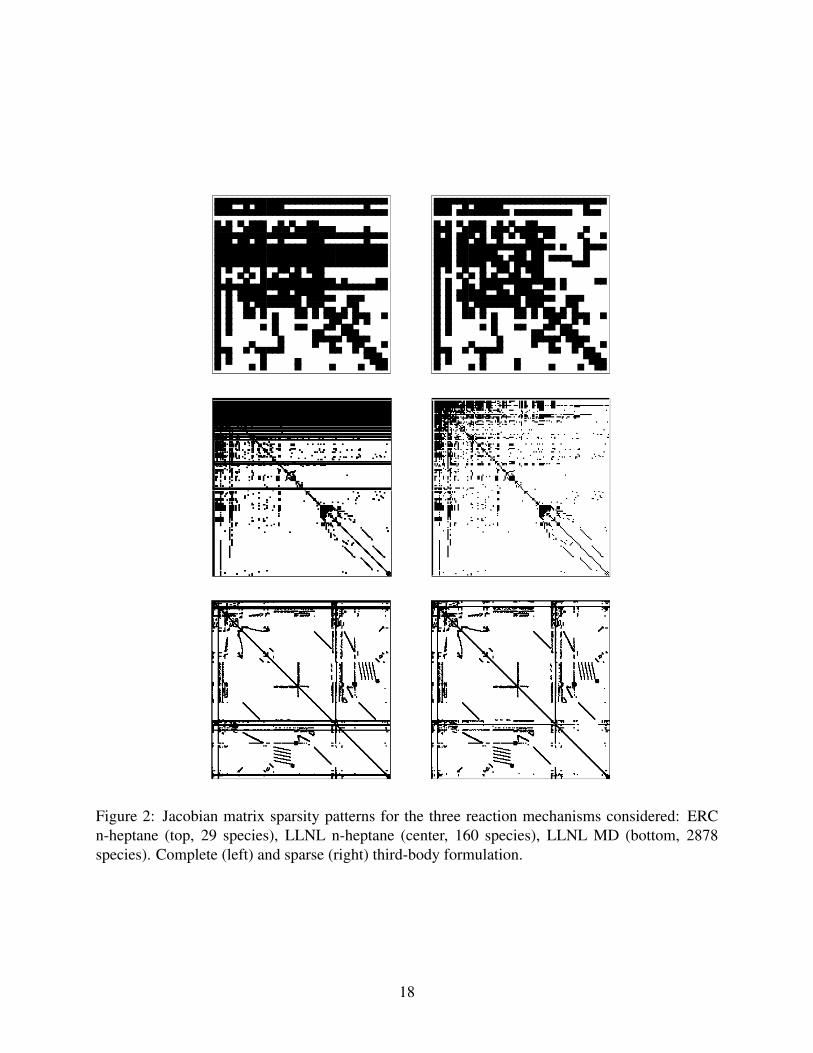
Figure 2: Jacobian matrix sparsity patterns for the three reaction mechanisms considered: ERCn-heptane (top, 29 species), LLNL n-heptane (center, 160 species), LLNL MD (bottom, 2878species). Complete (left) and sparse (right) third-body formulation.

18

2.5

3.0

3.5te

/ n

spar

se

LLNL methyl-decanoate

80%

100%Jacobian sparsity

101

102

103

104

1.0

1.5

2.0

ns

nco

mp

let

ERC n-Heptane

LLNL n-Heptane

101

102

103

104

40%

60%

ns

Complete formulationSparse formulation

Figure 3: Comparison between complete and approximate Jacobian formulations, for the threemechanisms considered. Left: ratio between non-zero elements in the complete and in the sparserformulation. Right: Jacobian matrix sparsity, percentage of zero elements.

f = x− x0/(x1− x0) , (30)

y = f y1 +(1− f ) y0;

parabolic interpolation requires instead three tabulated value retrievals, plus eleven algebraic oper-

ations (5 sums, 6 multiplications):

y =12(

f 2− f)

y−1 +(1− f 2)y0 +

12(

f 2 + f)

y1. (31)

In case the more accurate, yet more computationally demanding degree 4 polynomial interpolation

is adopted, 5 points are needed to estimate the function value at point x = f , and 32 operations (12

sums, 20 multiplications):

19

y = y−2 ·f

12(

f 2−1)( f

2−1)

(32)

+ y−1 ·f3( f −1)

(2− f 2

2

)+ y0 ·

(f 2

4−1)(

f 2−1)

+ y1 ·f3( f +1)

(2− f 2

2

)+ y2 ·

f12(

f 2−1)( f

2+1).

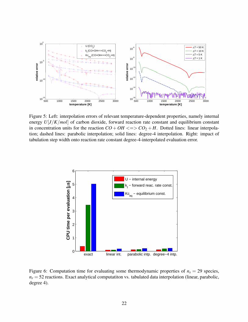
Figure 5 shows the interpolation error of three relevant thermodynamic functions for the carbon

dioxide species in the reaction of carbon monoxide with hydroxyl radical: species internal energy,

reaction equilibrium constant and forward reaction rate. The plots concerning each of the inter-

polated methods are for data tabulation at fixed ∆T = 10K, and plot the maximum interpolation

errors occurring at maximum distance between tabulation points. It can be observed that, whilst

linear and parabolic interpolation techniques yield standard relative accuracies, with relative errors

being significantly higher than the double precision machine accuracy, the degree-4 interpolation

is much more accurate, shrinking errors up to the order of machine precision. Also, even a wide

∆T = 10K fixed sampling interval step is shown to be highly accurate, yielding relative errors al-

ways lower than 10−10 for the forward reaction rate constants, which values span more than three

orders of magnitude in the evaluated temperature range. Considering that a full constant-volume

reactor simulation with analytical Jacobian computation includes 3 species-related and 7 reaction-

related temperature dependent quantities, which can be tabulated for computational efficiency, a

total storage requirement of the order O((3ns +7nr)ntab) needs to be provided whatever the inter-

polation method.

As represented in Figure 6, all of the interpolation methods provide an almost one-order-of-

magnitude wide computational time saving with respect to the exact, analytical computation of

20

the three tested temperature-dependent quantities. For this reason, the most accurate, degree 4

interpolation method has been chosen, with almost the same computational needs as the other in-

terpolation methods, and with the same storage requirements. A ∆T = 10K tabulation step, in

the overall temperature interval [500,3500]K has been chosen to provide better tradeoff between

interpolation error and memory storage requirements for all the variables to be tabulated. The high

accuracy degree of the 4th-order polynomial interpolation method also suggests that more accurate

interpolation techniques, which also require an evaluation of the function derivative in the tabu-

lation points, are less suitable as they would need twice the memory storage requirements than

standard polynomial interpolation.

yy

-1 1f x

y-1

y0

y1

y

01f x

y0

y1

y

0

y

y-1

y0 y1y

y2

y-2

-1 1f x0-2 2

Figure 4: Interpolation of tabulated data with constant sampling step: (in clockwise order) linearinterpolation, parabolic interpolation, degree 4 interpolation.

21

10-10

10-8

10-6

ve e

rro

r

T = 50 K

T = 10 K

T = 5 K

T = 1 K

10-5

100

ve e

rro

r

U (CO

2)

kf (CO+OH<=>CO

2+H)

Kceq

(CO+OH<=>CO2+H)

500 1000 1500 2000 2500 300010

-16

10-14

10-12

temperature [K]

rela

tiv

500 1000 1500 2000 2500 3000

10-15

10-10

temperature [K]

rela

tiv

Figure 5: Left: interpolation errors of relevant temperature-dependent properties, namely internalenergy U [J/K/mol] of carbon dioxide, forward reaction rate constant and equilibrium constantin concentration units for the reaction CO+OH <=> CO2 +H. Dotted lines: linear interpola-tion; dashed lines: parabolic interpolation; solid lines: degree-4 interpolation. Right: impact oftabulation step width onto reaction rate constant degree-4-interpolated evaluation error.

exact linear int. parabolic intp. degree−4 intp.0

1

2

3

4

5

6

CP

U t

ime

per

eva

luat

ion

[µs]

U − internal energy

kf − forward reac. rate const.

Kceq

− equilibrium const.

Figure 6: Computation time for evaluating some thermodynamic properties of ns = 29 species,nr = 52 reactions. Exact analytical computatiton vs. tabulated data interpolation (linear, parabolic,degree 4).

22

Results

Simulation setup

The analytical Jacobian formulation for the constant-volume problem has been implemented into a

software package for chemical kinetics computations, whose further details and validation have al-

ready been published.48 In particular, in order to test the accuracy and the computational efficiency

of the proposed approach, the three benchmark mechanisms of Table 1 have been adopted. The

first one by Patel et al.50 is a skeletal mechanism for n-heptane ignition consisting of 29 species and

52 reactions, used in internal combustion engine CFD simulations (e.g., Li and Kong54 and Park

and Reitz55), and is representative of small mechanisms, for which the Jacobian matrix is scarcely

sparse, and where the finite difference Jacobian approximation pursued by most ODE solvers is al-

ready a fairly efficient approach. The second mechanism51 is a mid-size mechanism consisting of

160 species and 1540 reactions, which provides a realistic degree of detail of n-heptane chemistry.

Due to its size, this mechanism has been be adopted in simplified, multi-zone or two-dimensional

simulations of kinetically-driven HCCI combustion (Guo et al.,56 Hoffman and Abraham57), but

needs to be reduced for practical internal combustion engine multidimensional simulations with

tens to hundreds of thousands of cells.58 The last, full methyl-decanoate reaction mechanism by

Herbinet et al.,4 consists of 2878 species and 8555 reactions, and represents a state-of-the-art

mechanism suitable for autoignition and flame simulations.

In order to provide a common simulation landscape for each of the mechanisms, 18 initial value

problems are simulated for each of them, corresponding to a matrix of cases involving two initial

reactor pressure values (p0 ∈{2.0;20.0}bar), three temperature values (T0 ∈{750;1000;1500}K),

and three initial lambda values of the air-fuel mixture (λ ∈ {0.5;1.0;2.0}).59,60 Each ignition case

is finally integrated for a time interval corresponding to about 1.5 times the mixture autoignition

time. Full details of the initialization matrix, including the species mass fractions, are given in

the Simulation Details Appendix. Each IVP integration interval has been subdivided into 100

23

partial steps in order to provide detailed time output in terms of reactor temperature and species

concentrations. This also simulates the integration conditions of the chemistry ODE system when

coupled to multidimensional CFD codes, where the species and internal energy source terms of

each cell are evaluated as part of an operator-splitting method,61 and thus the ODE solver is bound

to a usually small, fixed integration interval, of the order of 10−7 to 10−6 seconds.

ODE solver performance

The validation of the proposed formulation has been carried out by testing its performance when in-

tegrated through five different ODE solver packages tailored for stiff ODE systems, and compared

to a reference solution provided by the CHEMKIN-II package,62 and integrated using VODE.22

This choice has been made since CHEMKIN-II is a widely used open-source general purpose code

that has been applied to a variety of combustion chemistry simulations, including being integrated

in engine simulation codes, and thus it provides a suitable solution against which to compare other

codes. Access to the source code in CHEMKIN-II also makes it possible to directly compare its

performance by having control on the ODE solver integration parameters, the initialization over-

head and the solution output.

Relative and absolute integration error tolerances have been set at RTOL = 10−4, ATOL = 10−13,

equal for each integrated variable. As for the solver choice, the two LSODE solvers, in full

and sparse (LSODES) version,23 Hairer and Wanner’s implicit Runge-Kutta solver of order 5

RADAU5,63 the well known variable-coefficient VODE solver,22 and the DASPK integrator for

large systems of differential-algebraic equations,64 have been chosen. As far as DASPK is con-

cerned, the system of ODEs has been written in differential-algebraic residual form: G(t,y, y) =

y− f (t,y) = 0. This solver’s option to solve the linear system using the GMRES algorithm was

not used, as it requires the choice of a suitable preconditioner, that would make the integration not

comparable to the other solvers, which use direct solution by matrix decomposition.

The 18 IVP cases were run for each solver and combustion mechanism on an Intel core i7 920

24

-powered machine, with 8GB RAM memory, yielding a matrix of 270 cases to be compared.

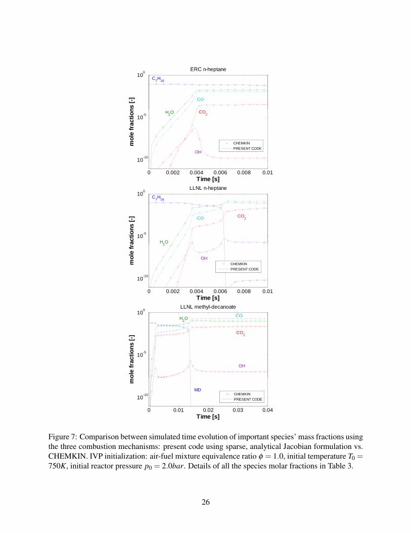
First of all, the code’s validation in analytical Jacobian form is provided in Figure 7, where the

simulation case number 2 is compared for each mechanism with the corresponding CHEMKIN

integration. It is an initial low temperature, low pressure case, where the system’s stiffness is at its

peak. In the plots, the actual integration configuration considers analytical Jacobians in the sparser

formulation, with degree 4 interpolation of tabulated temperature-dependent quantities, showing

excellent agreement between the time integration of the species’ mass fractions, and the corre-

sponding values arising from the CHEMKIN reference simulations.

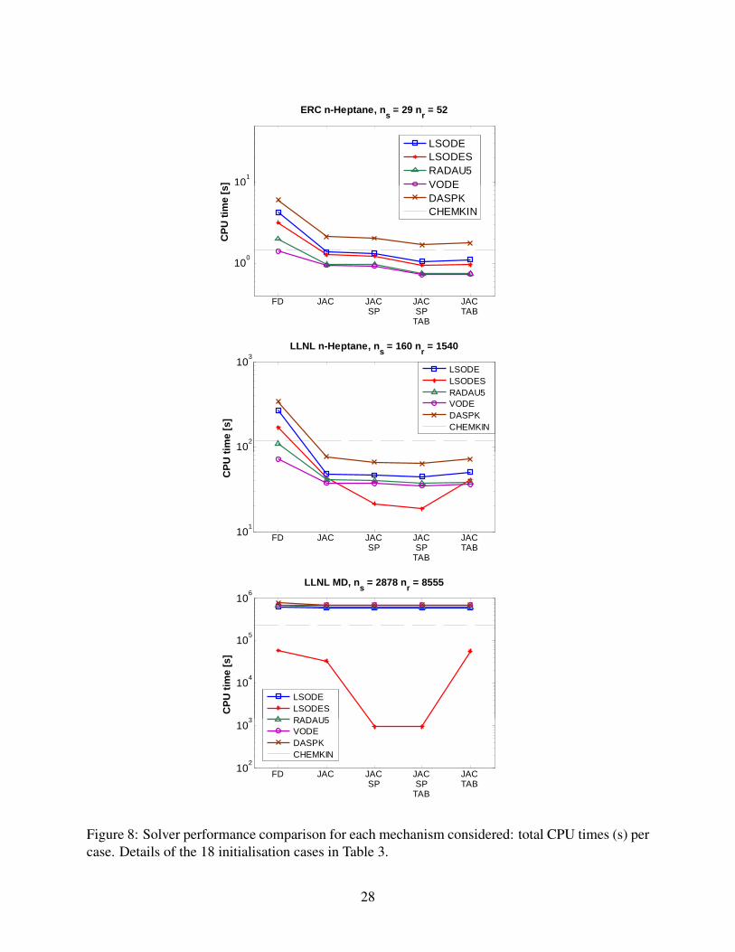
Figure 8 shows the solver comparison, in terms of overall CPU time summed over all the 18 cases.

It is seen that the present code, with VODE integration, has similar or better performance than the

CHEMKIN (VODE, too) even in the simplest form (i.e., exact temperature-dependent calculations

and finite-difference Jacobian form). When the analytical Jacobian formulation is chosen, a sig-

nificant improvement in total CPU times is observed, ranging from about 2 times with the smallest

mechanism, up to about 140 times with the huge one. The best simulation setup is always the one

considering sparse, analytical Jacobian, and interpolated functions.

As for the solver choice, it appears that the VODE and RADAU5 solvers provide optimum perfor-

mance when dealing with the smallest, almost dense mechanism, where the total integration times

are at least about 25% less than when using any other solver. When using medium and large mech-

anisms, instead, LSODES, the only solver in the set which uses sparse algebra for all the internal

operations, including computationally expensive matrix decompositions, always outperforms ev-

ery other solver, requiring from a minimum of 41% less CPU time (LLNL n-heptane mechanism)

up to reducing total time by more than two orders of magnitude (MD mechanism), although its

solution procedure is more dated.25

Performance of the DASPK integrator is shown to be similar to that of the LSODE solver; more-

over, the overall CPU times for the medium and large mechanisms are of the same order of the

other solvers which make use of full matrix algebra.

25

100

ERC n-heptane

ns

[-]

C

7H

16

CO

0 0.002 0.004 0.006 0.008 0.01

10-10

10-5

mo

le f

ract

ion

CHEMKIN

PRESENT CODE

CO2H

2O

OH

Time [s]

10-5

100

LLNL n-heptane

acti

on

s [-

]

C

7H

16

H2O

CO CO2

0LLNL methyl-decanoate

0 0.002 0.004 0.006 0.008 0.01

10-10

Time [s]

mo

le f

ra

CHEMKIN

PRESENT CODE

2

OH

10-5

100

ole

fra

ctio

ns

[-]

OH

CO2

COH

2O

0 0.01 0.02 0.03 0.04

10-10

Time [s]

mo

CHEMKIN

PRESENT CODE

MD

Figure 7: Comparison between simulated time evolution of important species’ mass fractions usingthe three combustion mechanisms: present code using sparse, analytical Jacobian formulation vs.CHEMKIN. IVP initialization: air-fuel mixture equivalence ratio φ = 1.0, initial temperature T0 =750K, initial reactor pressure p0 = 2.0bar. Details of all the species molar fractions in Table 3.

26

As for the internal integration details, Figures 9 and 10 show the counts of overall ODE func-

tion and Jacobian matrix evaluations required by the solver to complete the integration. In detail,

most differences between the cases descend from the different approach each solver has to the

integration. The RADAU5 implicit solver has on one hand really wide step sizes, but its high ac-

curacy order limits its computational efficiency as many function evaluations per step are needed.

The other solvers show similar numbers of integration steps, with the VODE being the least com-

putationally demanding in terms of Jacobian and function evaluations, thanks to variable order

and approximated Newton procedure. The number of residual function and Jacobian evaluations

needed by the DASPK integrator is at the upper part of the comparison with the other mechanisms.

In particular, at the low- and medium-size mechanisms the integration required approximately 20%

to 25% more residual function integrations, which lead to slightly greater overall CPU times.

As fas as polynomial interpolation for temperature-dependent functions is concerned, Tables

4,5,6 show that the accuracy of the interpolated functions is enough not to loosen the computa-

tional stability of the integration algorithms. The number of steps needed for the integrations,

where tabulated thermodynamic properties are adopted, is almost unchanged in comparison to the

corresponding cases which exploit exact analytical properties evaluation. Also, the CPU times

needed at the mechanism initialization stage, for tabulating thermodynamic properties, have been

measured for each of the three mechanisms tested. They added up to about 0.004 s, 0.104 s and

0.848 s for the ERC n-heptane, LLNL n-heptane and LLNL MD mechanisms, respectively; i.e.,

their impact in terms of CPU time has never been greater than 0.56% of the total integration time

of the fastest solver configuration.

Figure 11 finally shows the CPU times needed for the evaluation of the ODE system func-

tion and of the Jacobian matrix. It appears that the computational benefit due to interpolation is

dominant in the ODE function evaluation, while its impact is much lower on the evaluation of the

27

101

]

ERC n-Heptane, ns = 29 n

r = 52

LSODELSODESRADAU5VODE

100

FD JAC JAC

SPJACSP

TAB

JACTAB

CP

U t

ime

[s VODE

DASPKCHEMKIN

TAB

102

103

tim

e [

s]

LLNL n-Heptane, ns = 160 n

r = 1540

LSODELSODESRADAU5VODEDASPKCHEMKIN

LLNL MD, n = 2878 n = 8555

101

CP

U t

FD JAC JAC

SPJACSP

TAB

JACTAB

3

104

105

106

CP

U t

ime

[s]

LLNL MD, ns

2878 nr

8555

LSODELSODESRADAU5

102

103

FD JAC JAC

SPJACSP

TAB

JACTAB

RADAU5VODEDASPKCHEMKIN

Figure 8: Solver performance comparison for each mechanism considered: total CPU times (s) percase. Details of the 18 initialisation cases in Table 3.

28

6

7x 10

4

tio

ns

ERC n-Heptane, ns = 29 n

r = 52

LSODELSODESRADAU5VODEDASPK

3

4

5

Fu

nc

tio

n e

valu

a

FD JAC JAC

SPJACSP

TAB

JACTAB

CHEMKIN

TAB

6

6.5

7

7.5x 10

4

eva

luat

ion

s

LLNL n-Heptane, ns = 160 n

r = 1540

LSODELSODESRADAU5VODEDASPKCHEMKIN

4 LLNL MD, n = 2878 n = 8555

4

4.5

5

5.5

Fu

nc

tio

n e

FD JAC JAC

SPJACSP

TAB

JACTAB

5

5.5

6

6.5

7

7.5x 10

4

nc

tio

n e

valu

atio

ns

LLNL MD, ns

2878 nr

8555

LSODELSODESRADAU5VODEDASPKCHEMKIN

4

4.5

5

Fu

n

FD JAC JAC

SPJACSP

TAB

JACTAB

Figure 9: Solver performance comparison for each mechanism considered: number of functionevaluations. Details of the 18 initialisation cases in Table 3.

29

105

ati

on

s

ERC n-Heptane, ns = 29 n

r = 52

LSODELSODESRADAU5VODEDASPK

103

104

Jaco

bia

n e

valu

a

FD JAC JAC

SPJACSP

TAB

JACTAB

CHEMKIN

TAB

105

eva

lua

tio

ns

LLNL n-Heptane, ns = 160 n

r = 1540

LSODELSODESRADAU5VODEDASPKCHEMKIN

LLNL MD, n = 2878 n = 8555

103

104

Jaco

bia

n

FD JAC JAC

SPJACSP

TAB

JACTAB

104

105

cob

ian

eva

lua

tio

ns

LLNL MD, ns

2878 nr

8555

LSODELSODESRADAU5VODEDASPKCHEMKIN

103

Jac

FD JAC JAC

SPJACSP

TAB

JACTAB

Figure 10: Solver performance comparison for each mechanism considered: number of Jacobianevaluations. Details of the 18 initialisation cases in Table 3.

30

10−6

10−4

10−2

100

102

CP

U t

ime

[s]

FINITEDIFF.JAC.

COMPLETEANALYT.

JAC.

SPARSEANALYT.

JAC.

ODESYSTEM

FUN.

ERC n−heptLLNL n−heptLLNL MD

Figure 11: CPU time comparison for the evaluation of chemistry ODE system function and Jaco-bian matrix. Solid lines and filled marks indicate algebraic evaluation of temperature-dependentparameters, dash-dot lines and empty marks indicate tabulated temperature-dependent parameters.

Jacobian matrix, where also the difference in computational time between the complete and the

sparser formulation is negligible. Even though the sparser formulation does not include the contri-

bution of total mixture concentration to the derivative of the effective molecularity with respect to

species, which is a ns×1 array, the huge reduction in computational times achieved when using the

sparse Jacobian formulation is mainly due to a far less expensive matrix decomposition evaluation.

This behaviour is observed also when considering how the total CPU time savings are subdi-

vided between the three main features considered: adoption of analytical Jacobian, sparser formu-

lation for third-body reactions, and temperature-dependent data interpolation. From the analysis

shown in Figure 12, the analytical Jacobian formulation accomplishes for most of the CPU time

saving at all practical mechanism sizes (i.e., ns < 1000), where it can reach more than 80% of the

total speedup. The sparser three-body reactions formulation becomes very effective at the very

large mechanism sizes, where it can account for more than 50% the total speedup time, while its

effect is negligible for small and almost dense reaction mechanisms. Finally, as seen, polynomial

interpolation significantly reduces the CPU times for the evaluation of the ODE system function

and of the Jacobian matrix, and thus is significant in relative terms especially for the small mech-

31

101 102 103 1040

0.1

0.2

0.3

0.4

0.5

0.6

0.7

0.8

0.9

1

number of species, ns

CP

U ti

me

savi

ng fr

actio

n [−

]

Analytical JacobianSparser Jacobian formPolynomial interpolation

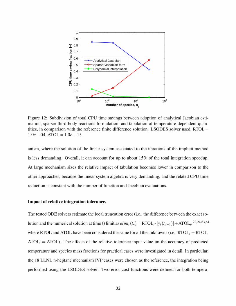
Figure 12: Subdivision of total CPU time savings between adoption of analytical Jacobian esti-mation, sparser third-body reactions formulation, and tabulation of temperature-dependent quan-tities, in comparison with the reference finite difference solution. LSODES solver used, RTOL =1.0e−04, ATOL = 1.0e−15.

anism, where the solution of the linear system associated to the iterations of the implicit method

is less demanding. Overall, it can account for up to about 15% of the total integration speedup.

At large mechanism sizes the relative impact of tabulation becomes lower in comparison to the

other approaches, because the linear system algebra is very demanding, and the related CPU time

reduction is constant with the number of function and Jacobian evaluations.

Impact of relative integration tolerance.

The tested ODE solvers estimate the local truncation error (i.e., the difference between the exact so-

lution and the numerical solution at time t) limit as elimi (tn)=RTOLi ·|yi (tn−1)|+ATOLi,22,24,63,64

where RTOL and ATOL have been considered the same for all the unknowns (i.e., RTOLi =RTOL,

ATOLi = ATOL). The effects of the relative tolerance input value on the accuracy of predicted

temperature and species mass fractions for practical cases were investigated in detail. In particular,

the 18 LLNL n-heptane mechanism IVP cases were chosen as the reference, the integration being

performed using the LSODES solver. Two error cost functions were defined for both tempera-

32

1010

1015

1020

1025

r v

alu

e

error (species)error (temperature)

25

30

35

40

tim

e [

s]

CPU time

105

106

integration stepsfunction evalsJacobian evalsmatrix decomp.

10-15

10-10

10-5

10-10

10-5

100

105

relative tolerance, RTOL

err

or

10-15

10-10

10-5

5

10

15

20

CP

U

10-15

10-10

10-5

103

104

relative tolerance, RTOL

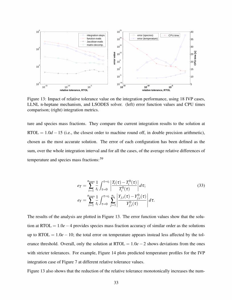
Figure 13: Impact of relative tolerance value on the integration performance, using 18 IVP cases,LLNL n-heptane mechanism, and LSODES solver. (left) error function values and CPU timescomparison; (right) integration metrics.

ture and species mass fractions. They compare the current integration results to the solution at

RTOL = 1.0d− 15 (i.e., the closest order to machine round off, in double precision arithmetic),

chosen as the most accurate solution. The error of each configuration has been defined as the

sum, over the whole integration interval and for all the cases, of the average relative differences of

temperature and species mass fractions:59

eT =ncases

∑i=1

1ti

∫τ=ti

τ=0

∣∣∣∣Ti(τ)−T 0i (τ)

T 0i (τ)

∣∣∣∣dτ; (33)

eY =ncases

∑i=1

1ti

∫τ=ti

τ=0

ns

∑j=1

∣∣∣∣∣Yj,i(τ)−Y 0j,i(τ)

Y 0j,i(τ)

∣∣∣∣∣dτ.

The results of the analysis are plotted in Figure 13. The error function values show that the solu-

tion at RTOL = 1.0e−4 provides species mass fraction accuracy of similar order as the solutions

up to RTOL = 1.0e− 10; the total error on temperature appears instead less affected by the tol-

erance threshold. Overall, only the solution at RTOL = 1.0e− 2 shows deviations from the ones

with stricter tolerances. For example, Figure 14 plots predicted temperature profiles for the IVP

integration case of Figure 7 at different relative tolerance values.

Figure 13 also shows that the reduction of the relative tolerance monotonically increases the num-

33

0 0.002 0.004 0.006 0.008 0.01700

800

900

1000

1100

1200

1300

1400

1500

1600

LLNL n−heptane, T0 = 750K, φ

0 = 1.0, p

0 = 2 bar

Time [s]

Tem

pera

ture

[K]

RTOL = 1.0d−02RTOL = 1.0d−04RTOL = 1.0d−08RTOL = 1.0d−15

Figure 14: Predicted temperature profiles for the IVP case of Figure 7, LLNL n-heptane mecha-nism, at different relative integration tolerance values.

ber of integration steps (and, similarly, of evaluations of the ODE system function), as the con-

straint for accepting a step on the local truncation error value becomes stricter. The corresponding

increase in the number of Jacobian matrix evaluations is instead smaller. This indicates that smaller

and more frequent integration steps, pursued at smaller relative tolerances, do not always make the

LSODES advancement algorithm require an update to the approximate Newton iterations’ Jacobian

matrix. Only in the RTOL range between 1.0e− 04 and 1.0e− 06, a greater number of Jacobian

matrix evaluations also appears to lead to a more accurate prediction in species mass fractions.

Comparison with other codes

The established performance of the proposed approach was compared to other available codes. In

particular, the same simulations per mechanism were run with the commercial code CHEMKIN-

PRO,65 and the open-source object-oriented package Cantera.66 A direct performance comparison

among these different programs is not possible, due to different management of IVP case input,

program output, since it is not possible to access all the solver parameters. However, the same

solution setup on each of the three codes were reproduced, i.e., each of the 18 IVP cases was

34

Table 2: Performance comparison among the present code, CHEMKIN-II, CHEMKIN-PRO, andCantera. Overall times for 18 IVP cases.

Code CPU Time [s]ERC n-heptane LLNL n-heptane LLNL MD

Present code 2.6 52.0 2312.0CHEMKIN-II 6.2 476.9 896099.Cantera 4.5 405.7 533939.CHEMKIN-PRO 16.0 46.0 2446.0

subdivided into 100 continuation runs, and hard-drive-intensive solution output was suppressed.

All the codes were run on a Pentium IV 3 GHz desktop machine. The performance comparison

results are summed up in Table 2. Apart from the small mechanism, where the performance of

CHEMKIN-PRO shows some initialization overhead, the presented solution approach yields very

similar CPU time performance to CHEMKIN-PRO for the two large mechanisms. No information

is available on how the preconditioned Krylov subspace method capability of the DASPK solver

– which appears to be used from the output of the CHEMKIN-PRO package – is implemented,

and if and which preconditioner is used. It is also not possible to compare the required numbers

of integration steps and of function and Jacobian evaluations per simulation. Finally, the Cantera

package, that implements the C language version of the VODE solver, appears less suitable for

simulations with large mechanisms, where management of the Jacobian matrix in full form leads

to significantly higher CPU times than the other two codes.

Internal combustion engine simulations.

In order to complete the validation of the accuracy and computational efficiency of the proposed

analytical Jacobian approach, the code has been coupled with the KIVA-4 code,61 for providing

engine CFD simulations with gas-phase reaction kinetics. In the code, a chemical kinetics ODE

system is evaluated in each cell of the computational grid and at each overall advancement time-

step. The chemistry solver interacts with the code by directly integrating the ODE system for

combustion chemistry over a time interval equal to the computational time-step defined by the

35

fluid flow solver. After the integration, the rates of change of species mass fractions due to chem-

istry are passed to the fluid flow solver, where they are introduced as part of an operator-splitting

approach. The effects of turbulence are accounted for at the resolved scales by the standard RNG

k− ε turbulence model, in terms of transport, mixing, and energy fluxes. This approach has been

shown to be accurate by Kokjohn and Reitz67 for predicting local mixture ignition and dynamics

for high- and low-temperature combustion regimes, including the short-delay high-temperature ig-

nition occurring in conventional direct injected diesel engines.

The validation of the chemistry solver coupling has been carried out considering a direct in-

jected diesel engine, featuring turbocharged air intake and a common-rail injection system working

at p = 1600bar target operating pressure. The full geometrical and operating details are reported

in the paper by Golovitchev et al.68 A computational grid consisting of 24780 cells at bottom dead

centre has been considered, and a reference full-load, maximum engine speed operating condition

has been chosen, where a single diesel fuel injection pulse is delivered into the combustion cham-

ber 25.20 crank angle degrees before top dead centre. Figure 15 shows the case’s validation using

either CHEMKIN or the present code for the detailed chemistry integration, adopting the skeletal

ERC n-heptane combustion mechanism.50 A high degree of accuracy in terms of both in-cylinder

pressure trace and instantaneous apparent rate of heat release is observed, with no differences be-

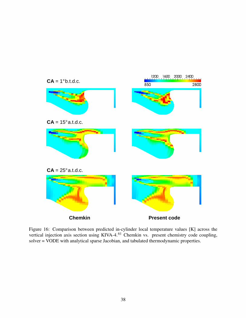
tween the two chemistry solvers. The temperature distribution in a vertical domain cross section

is shown in Figure 16, showing the computational accuracy of the present analytical Jacobian ap-

proach. The same simulation setup has also been run with the LLNL n-heptane mechanism for

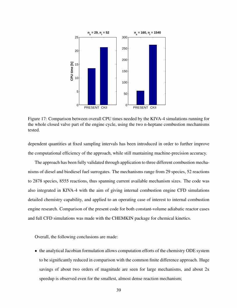
combustion chemistry. The overall computational times of the simulations are shown in Figure 17,

where significant time savings can be noted. The overall reductions in total CPU time are from

about 36% up to about 77% despite the fixed amount of time needed by the flow field solution

with a high number of species. This shows the possibility to adopt a semi-detailed reaction mech-

anism in internal combustion engine simulations, which can be completed in a reasonable amount

of time (i.e., approximately 60 hours, in this case), and without needing to reduce the combustion

36

0

20

40

60

80

100

120

140

160

180

2004000rpm, full load

In−c

ylin

der

pres

sure

(ba

r)

experiment

KIVA−4 − CHEMKIN

KIVA−4 − PRESENT CODE

0

15

30

45

60

75

90

105

120

135

150

Rat

e of

Hea

t Rel

ease

(J/

CA

)

−80 −60 −40 −20 0 20 40 60 80

min

j

CA degrees ATDC

Figure 15: Comparison between KIVA-461 calculation of a small, DI diesel engine of currentproduction. Chemkin62 vs. present chemistry code coupling, solver = VODE with analyticalsparse Jacobian, and tabulated thermodynamic properties.

mechanism further.

Concluding remarks

An analytical Jacobian approach for the efficient solution of general chemical kinetics initial value

problems involving arbitrary reaction mechanisms for the computation of combusting mixtures

has been developed. The methodology features evaluation of gas-phase mixture properties through

polynomial coefficients in JANAF standard format, and the computation of reaction rate constants

in various forms, including simple reactions following the modified Arrhenius kinetic law, third-

body reactions, and falloff reactions following Lindemann’s and Troe’s kinetic law forms.

An exact analytical formulation for the constant-volume adiabatic reactor, including the ODE

system’s Jacobian matrix, has been derived, and a further approximate form has been adopted,

which significantly increases the matrix sparsity pattern. Interpolation of tabulated temperature-

37

CA = 1°b.t.d.c.

CA = 15°a.t.d.c.

CA = 25°a.t.d.c.

Chemkin Present code

Figure 16: Comparison between predicted in-cylinder local temperature values [K] across thevertical injection axis section using KIVA-4.61 Chemkin vs. present chemistry code coupling,solver = VODE with analytical sparse Jacobian, and tabulated thermodynamic properties.

38

PRESENT CKII0

5

10

15

20

25

CP

U t

ime

[h]

ns = 29, n

r = 52

PRESENT CKII0

50

100

150

200

250

300

ns = 160, n

r = 1540

Figure 17: Comparison between overall CPU times needed by the KIVA-4 simulations running forthe whole closed valve part of the engine cycle, using the two n-heptane combustion mechanismstested.

dependent quantities at fixed sampling intervals has been introduced in order to further improve

the computational efficiency of the approach, while still mantaining machine-precision accuracy.

The approach has been fully validated through application to three different combustion mecha-

nisms of diesel and biodiesel fuel surrogates. The mechanisms range from 29 species, 52 reactions

to 2878 species, 8555 reactions, thus spanning current available mechanism sizes. The code was

also integrated in KIVA-4 with the aim of giving internal combustion engine CFD simulations

detailed chemistry capability, and applied to an operating case of interest to internal combustion

engine research. Comparison of the present code for both constant-volume adiabatic reactor cases

and full CFD simulations was made with the CHEMKIN package for chemical kinetics.

Overall, the following conclusions are made:

• the analytical Jacobian formulation allows computation efforts of the chemistry ODE system

to be significantly reduced in comparison with the common finite difference approach. Huge

savings of about two orders of magnitude are seen for large mechanisms, and about 2x

speedup is observed even for the smallest, almost dense reaction mechanism;

39

• the possiblility to exploit sparse matrix algebra for the Jacobian matrix computation en-

hanced the sparse LSODES solver capabilities, thus leading to significant computational

savings in comparison with other more efficient ODE solvers. This points out the need to

tailor the ODE solver to sparse algebra computations for maximum speed when dealing with

detailed combustion chemistry;

• tabulation of relevant temperature-dependent properties with a fourth-degree polynomial

function allowed high-fidelity representation of more complex functions involving compu-

tationally expensive exponentials, powers and logarithms, speeding their evaluation up by

almost one order of magnitude. The interpolation accuracy was enough not to affect the

stability of the integration algorithms tested;

• the most significant part of the speedup in comparison with the finite-difference Jacobian ap-

proach was due to the analytical Jacobian formulation. The impact of tabulation of temperature-

dependent quantities was significant especially for the small mechanism size, where linear

systems algebra was less demanding. The adoption of a sparser formulation for third-body

reactions instead showed greater effects for the largest mechanism, where it accounted for

more than 50% of the total CPU time reduction;

• coupling of present the chemistry code with CFD software for internal combustion engine

computations enabled detailed simulations with combustion mechanisms of dimensions of

the order of hundreds species to be completed reasonable time, of about one order of mag-

nitude less than the time required by standard chemistry packages.

• analytical knowledge of the Jacobian matrix sparsity structure for arbitrary chemical kinetics

problems also enables future work on to focus on the development of tailored ODE solution

procedures.

40

Appendix

Troe formulation

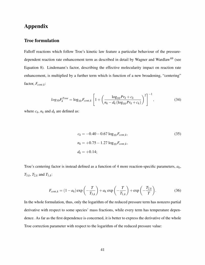
Falloff reactions which follow Troe’s kinetic law feature a particular behaviour of the pressure-

dependent reaction rate enhancement term as described in detail by Wagner and Wardlaw69 (see

Equation 8). Lindemann’s factor, describing the effective molecularity impact on reaction rate

enhancement, is multiplied by a further term which is function of a new broadening, “centering”

factor, Fcent,k:

log10FTroek = log10 Fcent,k

[1+(

log10 Prk + ck

nk−dk (log10 Prk + ck)

)2]−1

, (34)

where ck, nk and dk are defined as:

ck =−0.40−0.67 log10 Fcent,k, (35)

nk =+0.75−1.27 log10 Fcent,k,

dk =+0.14;

Troe’s centering factor is instead defined as a function of 4 more reaction-specific parameters, ak,

T3,k, T2,k and T1,k:

Fcent,k = (1−ak)exp(− T

T3,k

)+ak exp

(− T

T1,k

)+ exp

(−

T2,k

T

). (36)

In the whole formulation, thus, only the logarithm of the reduced pressure term has nonzero partial

derivative with respect to some species’ mass fractions, while every term has temperature depen-

dence. As far as the first dependence is concerned, it is better to express the derivative of the whole

Troe correction parameter with respect to the logarithm of the reduced pressure value:

41

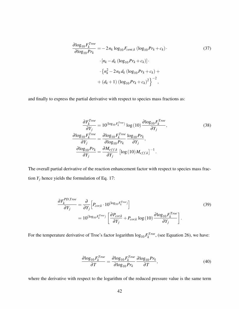
∂ log10 FTroek

∂ log10 Prk=−2nk log10 Fcent,k (log10 Prk + ck) · (37)

· [nk−dk (log10 Prk + ck)] ·

·{

n2k−2nk dk (log10 Prk + ck) +

+ (dk +1) (log10 Prk + ck)2}−2

,

and finally to express the partial derivative with respect to species mass fractions as:

∂FTroek

∂Yj= 10(log10 FTroe

k ) log(10)∂ log10 FTroe

k∂Yj

, (38)

∂ log10 FTroek

∂Yj=

∂ log10 FTroek

∂ log10 Prk

log10 Prk

∂Yj,

∂ log10 Prk

∂Yj=

∂Me f f ,k

∂Yj

[log(10)Me f f ,k

]−1.

The overall partial derivative of the reaction enhancement factor with respect to species mass frac-

tion Yj hence yields the formulation of Eq. 17:

∂FPD,Troek∂Yj

=∂

∂Yj

[Pcor,k ·10(log10 FTroe

k )]

(39)

= 10(log10 FTroek )

[∂Pcor,k

∂Y j+Pcor,k log(10)

∂ log10 FTroek

∂Yj

].

For the temperature derivative of Troe’s factor logarithm log10 FTroek , (see Equation 26), we have:

∂ log10 FTroek

∂T=

∂ log10 FTroek

∂ log10 Prk

∂ log10 Prk

∂T, (40)

where the derivative with respect to the logarithm of the reduced pressure value is the same term

42

as already computed in Equation 38, and

∂ log10 Prk

∂T=

1log(10)

[1

κ f ,k,0

∂κ f ,k,0

∂T− 1

κ f ,k,∞

∂κ f ,k,∞

∂T

]. (41)

Derivation of species thermodynamic properties

The needed thermodynamic properties of the species for solving the chemical kinetics IVP, and

their derivative expressions, are reported here. The JANAF 7-coefficient polynomial standard47

features two different coefficient sets {a,b, ...,g} for fitting two different temperature ranges.

Species internal energy[Jmol−1] and derivative (constant-volume specific heat)

[Jmol−1K−1]:

Ui = Rmol

[(ai−1)T +

bi

2T 2 +

ci

3T 3 +

di

4T 4 +

ei

5T 5 + fi

]; (42)

Cv,i =∂Ui

∂T= Rmol

[ai−1+bi T + ci T 2 +di T 3 + ei T 4] ;

constant volume specific heat’s derivative[Jmol−1K−2]:

∂Cv,i

∂T= Rmol

[bi +2ciT +3diT 2 +4eiT 3] . (43)

Standard non-dimensional Gibbs free energy [−] and derivative[K−1]:

g0i =−

[ai (logT −1)+

bi

2T +

ci

6T 2 +

di

12T 3 +

ei

20T 4− fi

T+gi

]; (44)

∂g0i

∂T=−

[ai

T+

bi

2+

ci

3T +

di

4T 2 +

ei

5T 3 +

fi

T 2

].

43

Simulation details

Table 3 summarizes the eighteen test case initialisation for the n-heptane and methyl-decanoate

combustion mechanisms. The results are tabulated in Tables 4, 5, 6, in terms of overall CPU

time, and solvers’ total number of integration steps and calls to the ODE system function, to the

Jacobian function, plus matrix decompositions. Data have been gathered exploiting the solvers’

optional output features, plus calls to the Fortran intrinsic cpu_time routine for the evaluation of

elapsed times. The number of calls to the ODE system function do not include those required for

building the Jacobian matrix, in case its internal generation by finite differences is selected.

44

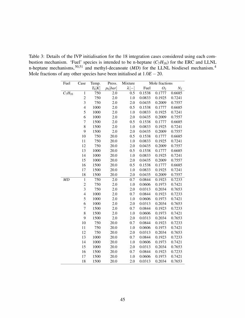
Table 3: Details of the IVP initialisation for the 18 integration cases considered using each com-bustion mechanism. ‘Fuel’ species is intended to be n-heptane (C7H16) for the ERC and LLNLn-heptane mechanisms,50,51 and methyl-decanoate (MD) for the LLNL biodiesel mechanism.4

Mole fractions of any other species have been initialised at 1.0E−20.

Fuel Case Temp. Press. Mixture Mole fractionsT0[K] p0[bar] λ [−] Fuel O2 N2

C7H16 1 750 2.0 0.5 0.1538 0.1777 0.66852 750 2.0 1.0 0.0833 0.1925 0.72413 750 2.0 2.0 0.0435 0.2009 0.75574 1000 2.0 0.5 0.1538 0.1777 0.66855 1000 2.0 1.0 0.0833 0.1925 0.72416 1000 2.0 2.0 0.0435 0.2009 0.75577 1500 2.0 0.5 0.1538 0.1777 0.66858 1500 2.0 1.0 0.0833 0.1925 0.72419 1500 2.0 2.0 0.0435 0.2009 0.7557

10 750 20.0 0.5 0.1538 0.1777 0.668511 750 20.0 1.0 0.0833 0.1925 0.724112 750 20.0 2.0 0.0435 0.2009 0.755713 1000 20.0 0.5 0.1538 0.1777 0.668514 1000 20.0 1.0 0.0833 0.1925 0.724115 1000 20.0 2.0 0.0435 0.2009 0.755716 1500 20.0 0.5 0.1538 0.1777 0.668517 1500 20.0 1.0 0.0833 0.1925 0.724118 1500 20.0 2.0 0.0435 0.2009 0.7557

MD 1 750 2.0 0.7 0.0844 0.1923 0.72332 750 2.0 1.0 0.0606 0.1973 0.74213 750 2.0 2.0 0.0313 0.2034 0.76534 1000 2.0 0.7 0.0844 0.1923 0.72335 1000 2.0 1.0 0.0606 0.1973 0.74216 1000 2.0 2.0 0.0313 0.2034 0.76537 1500 2.0 0.7 0.0844 0.1923 0.72338 1500 2.0 1.0 0.0606 0.1973 0.74219 1500 2.0 2.0 0.0313 0.2034 0.7653

10 750 20.0 0.7 0.0844 0.1923 0.723311 750 20.0 1.0 0.0606 0.1973 0.742112 750 20.0 2.0 0.0313 0.2034 0.765313 1000 20.0 0.7 0.0844 0.1923 0.723314 1000 20.0 1.0 0.0606 0.1973 0.742115 1000 20.0 2.0 0.0313 0.2034 0.765316 1500 20.0 0.7 0.0844 0.1923 0.723317 1500 20.0 1.0 0.0606 0.1973 0.742118 1500 20.0 2.0 0.0313 0.2034 0.7653

45

Table 4: ERC n-heptane

SolverFormulation CPU Number of:

analyt. sparse data time integr. funct. Jac. matrixJac. third-b. tab. (s) steps evals. evals. fact.

CHEMKIN - - - 1.48 26009 39752 2051 13637

LSODE

- - - 4.26 25358 40193 11631 11631? - - 1.37 25157 39956 11568 11568? ? - 1.33 24916 39674 11494 11494? ? ? 1.06 25126 39949 11590 11590? - ? 1.10 25451 40268 11674 11674

LSODES

- - - 3.15 25608 42038 5284 11922? - - 1.28 25751 42261 5273 11968? ? - 1.23 25796 42207 5258 11880? ? ? 0.95 26041 42642 5295 12044? - ? 0.96 25938 42408 5274 11984

RADAU5

- - - 1.99 5290 36828 4044 5230? - - 0.97 4713 39122 3297 4713? ? - 0.96 4723 39378 3301 4723? ? ? 0.75 4721 39367 3300 4721? - ? 0.74 4714 39128 3298 4714

VODE

- - - 1.42 25989 39719 2050 13513? - - 0.95 25744 39487 2056 13571? ? - 0.93 25926 39793 2053 13520? ? ? 0.72 25884 39663 2058 13617? - ? 0.73 25969 39908 2059 13648

DASPK

- - - 5.99 32473 50402 16266 16266? - - 2.13 32501 50490 16285 16285? ? - 2.03 32796 50918 16278 16278? ? ? 1.68 32813 51016 16249 16249? - ? 1.77 32614 50648 16261 16261

46

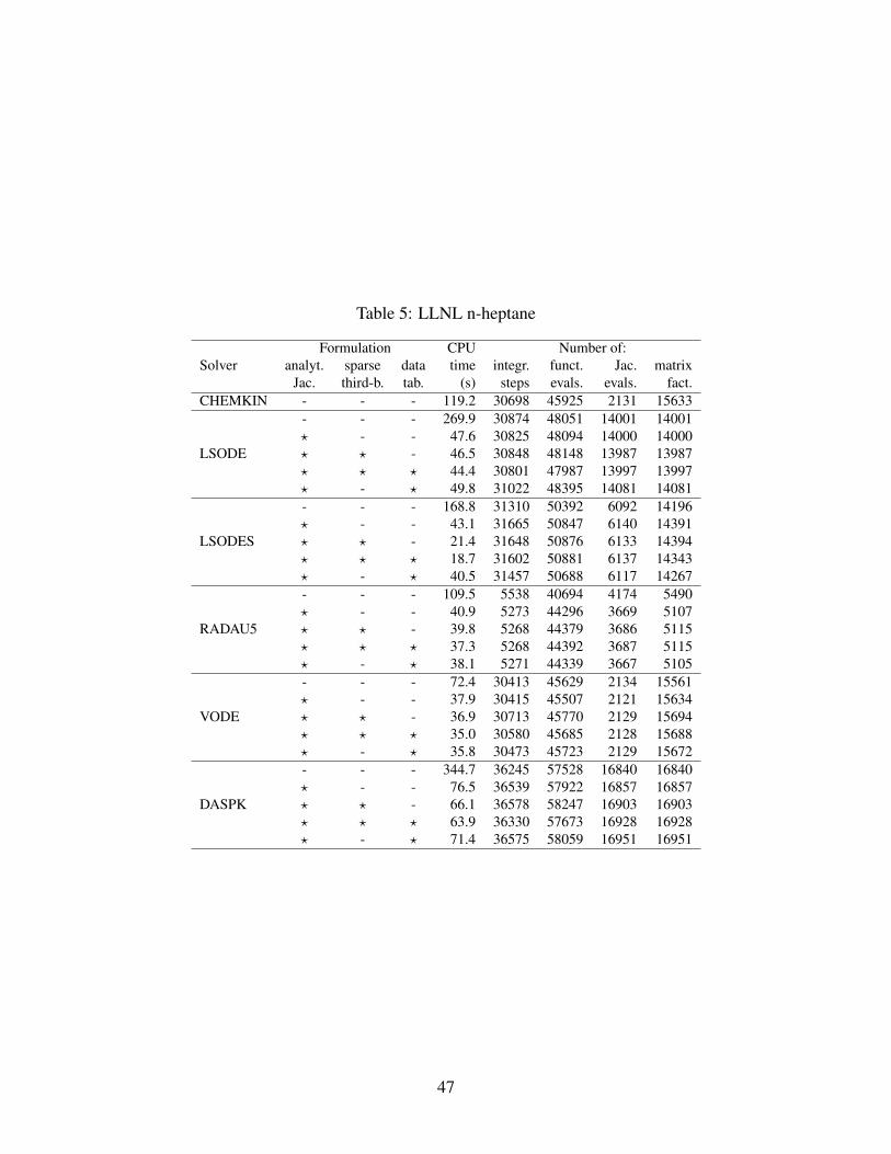
Table 5: LLNL n-heptane

SolverFormulation CPU Number of:

analyt. sparse data time integr. funct. Jac. matrixJac. third-b. tab. (s) steps evals. evals. fact.

CHEMKIN - - - 119.2 30698 45925 2131 15633

LSODE

- - - 269.9 30874 48051 14001 14001? - - 47.6 30825 48094 14000 14000? ? - 46.5 30848 48148 13987 13987? ? ? 44.4 30801 47987 13997 13997? - ? 49.8 31022 48395 14081 14081

LSODES

- - - 168.8 31310 50392 6092 14196? - - 43.1 31665 50847 6140 14391? ? - 21.4 31648 50876 6133 14394? ? ? 18.7 31602 50881 6137 14343? - ? 40.5 31457 50688 6117 14267

RADAU5

- - - 109.5 5538 40694 4174 5490? - - 40.9 5273 44296 3669 5107? ? - 39.8 5268 44379 3686 5115? ? ? 37.3 5268 44392 3687 5115? - ? 38.1 5271 44339 3667 5105

VODE

- - - 72.4 30413 45629 2134 15561? - - 37.9 30415 45507 2121 15634? ? - 36.9 30713 45770 2129 15694? ? ? 35.0 30580 45685 2128 15688? - ? 35.8 30473 45723 2129 15672

DASPK

- - - 344.7 36245 57528 16840 16840? - - 76.5 36539 57922 16857 16857? ? - 66.1 36578 58247 16903 16903? ? ? 63.9 36330 57673 16928 16928? - ? 71.4 36575 58059 16951 16951

47

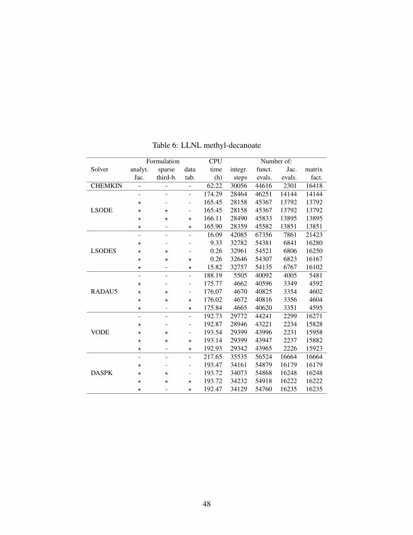
Table 6: LLNL methyl-decanoate

SolverFormulation CPU Number of:

analyt. sparse data time integr. funct. Jac. matrixJac. third-b. tab. (h) steps evals. evals. fact.

CHEMKIN - - - 62.22 30056 44616 2301 16418

LSODE

- - - 174.29 28464 46251 14144 14144? - - 165.45 28158 45367 13792 13792? ? - 165.45 28158 45367 13792 13792? ? ? 166.11 28490 45833 13895 13895? - ? 165.90 28359 45582 13851 13851

LSODES

- - - 16.09 42085 67356 7861 21423? - - 9.33 32782 54381 6841 16280? ? - 0.26 32961 54521 6806 16250? ? ? 0.26 32646 54307 6823 16167? - ? 15.82 32757 54135 6767 16102

RADAU5

- - - 188.19 5505 40092 4005 5481? - - 175.77 4662 40596 3349 4592? ? - 176.07 4670 40825 3354 4602? ? ? 176.02 4672 40816 3356 4604? - ? 175.84 4665 40620 3351 4595

VODE

- - - 192.73 29772 44241 2299 16271? - - 192.87 28946 43221 2234 15828? ? - 193.54 29399 43996 2231 15958? ? ? 193.14 29399 43947 2237 15882? - ? 192.93 29342 43965 2226 15923

DASPK

- - - 217.65 35535 56524 16664 16664? - - 193.47 34161 54879 16179 16179? ? - 193.72 34073 54868 16248 16248? ? ? 193.72 34232 54918 16222 16222? - ? 192.47 34129 54760 16235 16235

48

References

(1) Lu, T.; Law, C. K. Prog. Energy Combust. Sci. 2009, 35, 192 – 215.

(2) Miller, J. A.; Kee, R. J.; Westbrook, C. K. Annu. Rev. Phys. Chem. 1990, 41, 345–387.

(3) Law, C. K. Proc. Combust. Inst. 2007, 31, 1 – 29.

(4) Herbinet, O.; Pitz, W. J.; Westbrook, C. K. Combust. Flame 2008, 154, 507 – 528.

(5) Herbinet, O.; Pitz, W. J.; Westbrook, C. K. Combust. Flame 2010, 157, 893 – 908.

(6) Westbrook, C.; Pitz, W.; Westmoreland, P.; Dryer, F.; Chaos, M.; Osswald, P.; Kohse-

Höinghaus, K.; Cool, T.; Wang, J.; Yang, B.; Hansen, N.; Kasper, T. Proc. Combust. Inst.

2009, 32, 221 – 228.

(7) Westbrook, C. K.; Pitz, W. J.; Herbinet, O.; Curran, H. J.; Silke, E. J. Combust. Flame 2009,

156, 181 – 199.

(8) Seshadri, K.; Lu, T.; Herbinet, O.; Humer, S.; Niemann, U.; Pitz, W. J.; Seiser, R.; Law, C. K.

Proc. Combust. Inst. 2009, 32, 1067 – 1074.

(9) Kong, S.-C.; Reitz, R. D. Proc. Combust. Inst. 2002, 29, 663 – 669, Proceedings of the

Combustion Institute.

(10) Kong, S.-C.; Reitz, R. D. J. Eng. Gas Turbines Power 2002, 124, 702–707.

(11) Kokjohn, S. L.; Hanson, R. M.; Splitter, D. A.; Reitz, R. D. Int. J. Engine Res. 2011, 12,

209–226.

(12) Kokjohn, S.; Hanson, R.; Splitter, D.; Kaddatz, J.; Reitz, R. SAE Int. J. Engines 2011, 4,

360–374.

(13) Maas, U.; Pope, S. Combust. Flame 1992, 88, 239 – 264.

(14) Lam, S.; Coussis, D. Symp. (Int.) Combust. 1989, 22, 931 – 941.

49

(15) Lu, T.; Law, C. K. Proc. Combust. Inst. 2005, 30, 1333 – 1341.

(16) Lu, T.; Law, C. K. Combust. Flame 2006, 144, 24 – 36.

(17) Lu, T.; Law, C. K. Combust. Flame 2006, 146, 472 – 483.

(18) Lu, T.; Law, C. K.; Yoo, C. S.; Chen, J. H. Combust. Flame 2009, 156, 1542 – 1551.

(19) Sun, W.; Chen, Z.; Gou, X.; Ju, Y. Combust. Flame 2010, 157, 1298 – 1307.

(20) Curtiss, C. F.; Hirschfelder, J. O. Proc. Natl. Acad. Sci. U. S. A. 1952, 38, 235–243.

(21) Gear, C. W. Numerical Initial Value Problems in Ordinary Differential Equations; Prentice

Hall PTR: Upper Saddle River, NJ, USA, 1971.

(22) Brown, P. N.; Byrne, G. D.; Hindmarsh, A. C. SIAM J. Sci. Stat. Comp. 1989, 10, 1038–1051.

(23) Hindmarsh, A. IMACS Transactions on Scientific Computation 1983, 1, 55–64.

(24) Hindmarsh, A. C. ACM SIGNUM Newsletter 1980, 15, 10–11.

(25) Byrne, G. D.; Dean, A. M. Comput. Chem. 1993, 17, 297 – 302.

(26) Aro, C. J. Comput. Phys. Commun. 1996, 97, 304 – 314.

(27) Kim, S.-L.; Choi, J.-Y.; Jeung, I.-S.; Park, Y.-H. Appl. Numer. Math. 2001, 39, 87 – 104.

(28) Aro, C. J.; Rodrigue, G. H. Comput. Phys. Commun. 1995, 92, 27 – 53.

(29) Aro, C. J. Appl. Numer. Math. 1996, 21, 335 – 352.

(30) Nejad, L. A. M. Astrophys. Space Sci. 2005, 299, 1–29, 10.1007/s10509-005-2100-z.

(31) Carver, M. B.; Boyd, A. W. J. Phys. Chem. 1979, 11, 1097–1108.

(32) Sandu, A.; Verwer, J.; Blom, J.; Spee, E.; Carmichael, G.; Potra, F. Atmos. Environ. 1997, 31,

3459 – 3472.

50

(33) Sandu, A.; Verwer, J.; Loon, M. V.; Carmichael, G.; Potra, F.; Dabdub, D.; Seinfeld, J. Atmos.

Environ. 1997, 31, 3151 – 3166, EUMAC: European Modelling of Atmospheric Constituents.

(34) Bisetti, F. Combust. Theory Modell. 2012, 16, 387–418.

(35) Sandu, A.; Sander, R. Atmos. Chem. Phys. 2006, 6, 187–195.

(36) Damian, V.; Sandu, A.; Damian, M.; Potra, F.; Carmichael, G. R. Comput. Chem. Eng. 2002,

26, 1567 – 1579.

(37) Bank, R.; Douglas, C. Adv. Comput. Math. 1993, 1, 127–137, 10.1007/BF02070824.

(38) Remington, K.; Pozo, R. NIST Sparse BLAS User’s Guide; 1996.

(39) Brown, P. N.; Hindmarsh, A. C. Appl. Math. Comput. 1989, 31, 40 – 91, Special Issue Nu-

merical Ordinary Diferrential Equations (Proceedings of the 1986 ODE Conference).

(40) Barz, T.; Kuntsche, S.; Wozny, G.; Arellano-Garcia, H. Comput. Chem. Eng. 2011, 35, 2053

– 2065.

(41) Buzzi Ferraris, G.; Manca, D. Comput. Chem. Eng. 1998, 22, 1595 – 1621.

(42) Tolsma, J. E.; Barton, P. I. Comput. Chem. Eng. 1998, 22, 475 – 490.

(43) Tolsma, J.; Barton, P. I. Ind. Eng. Chem. Res. 2000, 39, 1826–1839.

(44) Schwer, D. A.; Tolsma, J. E.; Green, W. H.; Barton, P. I. Combust. Flame 2002, 128, 270 –

291.

(45) Mosbach, S.; Kraft, M. Combust. Theory Modell. 2006, 10, 171–182.

(46) Lee, S. L.; Gear, C. W. J. Comput. Appl. Math. 2007, 201, 258 – 274.

(47) M. W. Chase, J.; Curnutt, J. L.; J. R. Downey, J.; McDonald, R. A.; Syverud, A. N.; Valen-

zuela, E. A. J. Phys. Chem. Ref. Data 1982, 11, 695–940.

51

(48) Perini, F. Optimally reduced reaction mechanisms for Internal Combustion En-

gines running on biofuels. Ph.D. thesis, University of Modena and Reggio Emilia,

http://www.himech-phdschool.unimore.it/site/home/download/

tesi-di-dottorato/documento92016812.html, 2011.

(49) Warnatz, J.; Warnatz, J.; Maas, U.; Dibble, R.; Dibble, R. Verbrennung: Physikalisch-

Chemische Grundlagen, Modellierung und Simulation, Experimente, Schadstoffentstehung;

Springer, 2001.

(50) Patel, A.; Kong, S.; Reitz, R. Development and Validation of a Reduced Reaction Mechanism

for HCCI Engine Simulations. 2004; http://papers.sae.org/2004-01-0558/.

(51) Seiser, R.; Pitsch, H.; Seshadri, K.; Pitz, W.; Curran, H. Proc. Combust. Inst. 2000, 28, 2029

– 2037.

(52) Yamamoto, A.; Kitamura, Y.; Yamane, Y. Ann. Nucl. Energy 2004, 31, 1027 – 1037.

(53) Schraudolph, N. N. Neural Comput. 1999, 11, 853–862.

(54) Li, Y. H.; Kong, S.-C. Combust. Theory Modell. 2008, 12, 205–219.

(55) Park, S. W.; Reitz, R. D. Fuel 2009, 88, 843 – 852.

(56) Guo, H.; Li, H.; Neill, W. S. ASME ICEF2009 Conference Proceedings 2009, 2009, 489–497.

(57) Hoffman, S. R.; Abraham, J. Fuel 2009, 88, 1099 – 1108.

(58) Shi, Y.; Ge, H.-W.; Brakora, J. L.; Reitz, R. D. Energy Fuels 2010, 24, 1646–1654.

(59) Perini, F.; Brakora, J. L.; Reitz, R. D.; Cantore, G. Combust. Flame 2012, 159, 103 – 119.

(60) Perini, F.; Cantore, G.; Reitz, R. An Analysis on Time Scale Separation for Engine Simula-

tions with Detailed Chemistry. 2011; http://papers.sae.org/2011-24-0028.

(61) Torres, D. J.; Trujillo, M. F. J. Comput. Phys. 2006, 219, 943 – 975.

52

(62) Kee, R. J.; Rupley, F. M.; Miller, J. A. CHEMKIN-II: A FORTRAN Chemical Kinetics Pack-

age for the Analysis of Gas-Phase Chemical Kinetics; 1989.

(63) Hairer, E.; Wanner, G. Solving Ordinary Differential Equations II: Stiff and differential-

algebraic problems; Springer series in computational mathematics; Springer-Verlag, 1993.

(64) Brown, P. N.; Hindmarsh, A. C.; Petzold, L. R. SIAM J. Sci. Comput. 1994, 15, 1467–1488.

(65) http://www.reactiondesign.com/products/open/chemkin-pro.html.

(66) Goodwin, D. Chemical Vapor Deposition XVI and EUROCVD 14 (2003) 2003, 2003-08,

155–162.

(67) Kokjohn, S. L.; Reitz, R. D. J. Eng. Gas Turbines Power 2011, 133, 102805.

(68) Golovitchev, V. I.; Montorsi, L.; Rinaldini, C. A.; Rosetti, A. ASME ICEF2006 Conference

Proceedings 2006, 2006, 349–358.

(69) Wagner, A. F.; Wardlaw, D. M. J. Phys. Chem. 1988, 92, 2462–2471.

53