Comments Welcome

An Anatomy of Pairs Trading:

the role of idiosyncratic news, common information and liquidity

Joseph Engelberg, Pengjie Gao and Ravi Jagannathan�y

First Draft: August, 2007This Draft: September 18, 2008

Abstract

In this paper, we examine the pro�tability from a convergence trading strategy called pairs

trading which bets that a pair of stocks with price paths that have historically moved together

will eventually converge if they ever diverge. We �nd that the pro�tability from pairs trading

is greatest soon after the pairs diverge and that the pro�tability is strongly related to events

around the date of divergence. Pro�tability is low when there is idiosyncratic news about a

stock in the pair and high when there is an idiosyncratic liquidity shock to a stock in the pair.

When there is information common to both stocks in the pair, we �nd that the pro�ts to pairs

trading can be high when frictions cause this information to be more quickly incorporated into

one stock in the pair and not the other. We further show how idiosyncratic news, common

information and liquidity are systematically related to horizon risk, divergence risk and the speed

of convergence of the pairs trading, which illustrates some subtle trade-o¤s faced by arbitragers

when attempting to arbitrage such potential mispricing. (JEL Classi�cation: G11, G12, G14)

�We are grateful to Robert Battalio, Shane Corwin, Tom Cosimano, Zhi Da, Levent Guntay, Tim Loughran,Todd Pulvino, Paul Schultz, Sophie Shive, and several empolyees at Lehman Brothers for helpful discussions andcomments. We also thank seminar participants at the University of Notre Dame and the Indiana-Purdue-Notre DameJoint Conference on Finance for valuable feedback. The Zell Center for Risk Management and the Financial Marketand Institution Center provided partial funding for this research. All errors are our own.

yCorrespondence: Joseph Engelberg, Finance Area, Kenan Flagler Business School, University of North Carolinaat Chapel Hill; Pengjie Gao, Finance Department, Mendoza College of Business, University of Notre Dame; and RaviJagannathan, Finance Department, Kellogg School of Management, Northwestern University and NBER. E-mail:joseph_engelberg@kenan-�agler.unc.edu, pgao@nd.edu, and rjaganna@kellogg.northwestern.edu.

1 Introduction

Financial economists have long been interested in understanding the pro�tability underlying var-

ious forms of statistical arbitrages for two reasons. First, in the debate over whether �nancial

markets are e¢ cient, such strategies violate the weakest form of market e¢ ciency as de�ned by

Fama (1970). Second, these strategies help some �nancial economists better understand the mar-

ket frictions or behavioral biases that cause prices to deviate from fundamental values (Barberis,

Shleifer and Vishny, 1998; Daniel, Hirshleifer and Subramayahm, 1998; Hong and Stein, 1999)

and they help others identify risk factors that explain the underlying pro�tability as compensa-

tion for bearing risk (Berk, Naik and Green, 1999). We have collectively identi�ed strong return

predictability over various horizons from strategies based on the historical price path of individual

stocks. These strategies consider the past performance of stocks in isolation in order to predict

future price performance. Such statistical arbitrage can be loosely classi�ed into (1) short-term

reversal strategies (Jegadeesh, 1990; Lehmann, 1990); (2) intermediate-term relative strength or

price momentum strategies (Jegadeesh and Titman, 1993), and (3) long-term reversal strategies

(De Bondt and Thaler, 1985). Since the pro�tability of these strategies has been documented many

papers have sought to understand the source of pro�tability in these strategies.1

Far less attention has been given to relative return strategies - which also violate weak form

e¢ ciency � and what these strategies tell us about market imperfections. With the idea that

stocks may be cointegrated (Bossaerts, 1988), these strategies consider the past performance of

stocks relative to other stocks in order to predict future price performance. One popular strategy

is called �pairs trading.� 2 The idea behind pairs trading is to �rst identify a pair of stocks with

similar historical price movement. Then, whenever there is su¢ cient divergence between the prices

in the pair, a long-short position is simultaneously established to bet that the pair�s divergence

is temporary and that it will converge over time. Recently, Gatev, Goetzmann and Rouwenhorst

(2006, hereafter GGR) showed that a pairs trading strategy generates annual returns of 11 percent

and a monthly Sharpe ratio four to six times that of market returns between 1962 and 2002.3

Despite these large risk-adjusted returns, we know very little about why pairs trading is prof-

itable. For example, what causes the pairs to diverge? Is the cause of the divergence related to the

subsequent convergence? What determines the speed and horizon of the pairs�convergence? What

precludes market participants from eliminating such mispricing? The purpose of this paper is to

shed some light on these questions.4 We have four key �ndings. First, after a pair has diverged the

1For example, since the seminal paper on price momentum was published by Jagadeesh and Titman (1993), 130papers in the Journal of Finance, Journal of Financial Economics and Review of Financial Studies has cited thepaper. Only seven other papers published after it have more citations in these three journals.

2Several strategies are similar to the pairs trading. Instead of relying on the statistical relationship betweenhistorical prices as in the pairs trading, these strategies consider relative pricing of shares due to di¤erences intrading locations (Froot and Dabora, 1999; Scruggs, 2006), or di¤erences in cash�ow rights and voting rights (Smithand Amoako-Adu, 1995; Zingales, 1995).

3Schultz and Shive (2008) show that the dual-class share arbitrage - which has some similarities to pairs trading- also generates economically returns after taking into account the �rst-order transaction costs during the years 1993to 2006.

4Little empirical work to date has directly investigated pairs trading. Harris (2002) discusses the implementation

1

pro�tability from the pair decreases exponentially over time. A strategy which commits to closing

each position within 10 days of divergence increases the average monthly return to pairs trading

from 70 bps per month to 175 bps per month (before transaction costs) without any increase in the

number of trades. Second, we �nd that the pro�ts to a pairs trading strategy are related to news

around the divergence event. We identify idiosyncratic news events from articles in the Dow Jones

News Service and �nd that when a pair diverges because of �rm-speci�c news, the divergence is

more likely to be permanent and hence the pro�tability to a pairs trading strategy is lower. Third,

we �nd that the pro�tability to pairs trading is related to information events that a¤ect both �rms

in the pair (�common shocks�). Using a measure of information di¤usion at the industry level

we �nd some of the pro�tability to pairs trading can be explained by a di¤erential response to

these common information shocks and that this di¤erential response is related to di¤erent liquidity

levels of the constituent stocks. Fourth, we �nd the pro�tability from pairs trading is smaller when

institutional investors hold both of the constituent �rms in a pair and sell-side analysts cover both

of the constituent �rms. Taken together, our results suggest that the pro�ts to pairs trading are

short-lived and directly related to information di¤usion across the constituent �rms of the pair.

When information about a �rm is idiosyncratic, it does not a¤ect its paired �rm and thus creates

permanent di¤erences in prices. When information is common, market frictions like illiquidity and

costly information acquisition create a lead-lag relationship between the return patterns of the

constituent �rms that leads to pro�tability in the form of a pairs trading strategy.

The rest of the paper is organized as follows. Section 2 illustrates how to implement the pairs

trading strategy based on the historical price relationship following GGR. Section 3 reviews the

related literatures and develops our research questions. Section 4 describes the sources of data

used in this study and provides some summary statistics of the main variables. Section 5 provides

time-series evidence of how the pro�ts from pairs trading are related to some pair characteristics,

including �rm-speci�c news, industry-wide common information, long-run liquidity level and short-

term liquidity shocks, as well as the structure of the underlying institutional ownership and the

information intermediary. Section 6 explores the risk and return pro�les of pairs trading in a cross-

sectional regression framework, and explores the divergence risk and horizon risk associated with

pairs trading. Section 7 carries out a set of robustness checks. Section 8 summarizes and concludes.

2 Implementation of Pairs Trading Strategy

Executing the simplest form of the pairs trading strategy involves two steps. First, we match pairs

based on normalized price di¤erences over a one year period. We call this the �estimation period�.

Speci�cally, from the beginning of the year, on each day t , we compute each individual stock�s

of pairs trading and provides several examples. Andrade, di Pietro and Seashole (2005) construct sixteen pairs usingstocks traded on the Tiwan Stock Exchange following the procedure in GGR, they and �nd out-of-sample evidenceon pro�tability. They also show the trading of retail investors may a¤ect the probability that a pair opens. Ourpaper is much di¤erent. Our paper is a large-scale investigation into the role that information and liquidity play inthe pro�tability of pairs trading. In addition, we propose a set of econometric techniques to characterize the risksand return pro�les of pairs trading.

2

normalized price (P it ) as

P it =tY

�=1

1��1 + ri�

�(1)

where P it is stock i�s normalized price by the end of day t , � is the index for all the trading days

between the �rst trading day of the year till day t , and ri� is the stock�s total return (dividends

included) on day � . To ensure the set of stocks involved in pairs trading are relatively liquid,

we exclude all stocks with one or more days without trades during the estimation period. After

obtaining the normalized price series for each stock, at the end of the year, we compute the following

squared normalized price di¤erence measure between stock i and stock j,

PDi;j =

NtXt=1

�P it � P

jt

�2(2)

where PDi;j is the squared normalized price di¤erence measure between stock i and stock j, Nt is

the total number of trading days in the estimation period, P it and Pjt are the normalized prices for

stock i and stock j respectively on trading day t . One can also compute the standard deviation

of the normalized price di¤erences,

StdPDi;j =1

Nt � 1

NtXt=1

��P it � P

jt

�2��P it � P

jt

�2�(3)

The next step during the estimation period is to identify pairs with the minimal normalized

price di¤erences. If there are N stocks under consideration, we need to compute N � (N � 1) =2normalized price di¤erences, which potentially could be a very large number. We choose to consider

pairs from the same industry. In particular, we use the Fama-French twelve-industry industry clas-

si�cation scheme (Fama and French, 1997), and compute the pairwise normalized price di¤erence.

We then pool all the pairs together and rank these pairs based on the pairwise normalized price

di¤erence.

During the following year which we call the �eligibility period�, each month, we consider the

200 pairs with the smallest normalized price di¤erence taken from the estimation period. If the

stocks in the pair diverge by more than two standard deviations of the normalized price di¤erence

established during the estimation period then we buy the �cheap� stock in the pair and sell the

�expensive�one. As in GGR, we wait one day after divergence before investing in order to mitigate

the e¤ects of bid-ask bounce and other market microstructure induced irregularities.5 If the pair

5One such irregularity is a trading halt. Lee, Ready, and Seguin (1994), Corwin and Lipson (2000), Christie,Corwin and Harris (2002) show that trading halts are usually associated with large price changes. For example, TableII of Christie, Corwin and Harris (2002) shows 97:8% of trading halts related to average absolute price changes of5:48%. Table I in the same paper shows that the resolution of trading halts for a sample Nasdaq stocks within thesame day accounts for about 85% of the cases, about 99% by the time of opening on the second day, and 100% by theend of the next trading day. As we discuss in the later part of this paper, one reliable determinant on the openingof the pairs is the news, one may be concerned about the measurement of returns during such period. Based on theabove evidence, skipping a day will resolve incomplete adjustment of prices during such irregular trading scenarios.

3

later converges we unwind our position and wait for the pair to diverge again. If the pair diverges

but does not converge within 6 months, we close the position and call this �no convergence.� In

section 5, we consider a �cream-skimming� strategy which closes the position on pairs that have

not converged within 10 days.

We calculate buy-and-hold portfolio returns to the pairs trading strategy as in GGR to avoid

the transaction cost associated with daily rebalancing. Let p(li; si) �which we will write as pi for

brevity �indicate the pair of stock li and stock si for the pair. We let Di indicate the most recent

day of divergence for pair pi . When we invest in the pair one day after divergence, we let the �rst

coordinate (l) indicates the stock in which we go long and the second coordinate (s) indicates the

stock in which we go short. We indicate the return to stock li on day t as Rt(li) and the return to

stock si on day t as Rt(si) so that the return for pi on day t is de�ned as,

Rt(pi) = Rt(l

i)�Rt(si) (4)

then the return to a portfolio of N pairs on day t is

RPortfoliot =

NXi=1

W itRt(p

i) (5)

where the weight W it is de�ned as

W it =

$itPNj=1$

jt

;

and

$jt = (1 +Rt�1(pj))� (1 +Rt�2(pj))� :::� (1 +RDi+1(p

j)) :

In words, we use the N pairs that are held in the portfolio on day t , and calculate the daily

return to the portfolio as the weighted average of the returns to the N pairs on day t but the

weight ($it ) given to the return of pair i on day t is determined by its cumulative return in the

portfolio ending on day t� 1 with respect to the other pairs.

3 Development of Research Questions

3.1 Pro�tability of Pairs Trading in Event-Time: Initial Evidence

Figure 1 graphs the mean pair-return in event-time where event day T is (T + 1) days after the

pair diverges (at day 0). Consistent with GGR, skipping a day after the divergence of the pair prior

to taking position mitigates microstructure e¤ects, such as the �rst-order negative serial correlation

induced by the bid-ask bounce. The �gure clearly illustrates the pro�tability from pairs trading

declines substantially in event time. For example, event day 1 and 2 generate a mean return of

23 and 13 basis points respectively but after event day 4 the mean pair-returns from pairs trading

never reach 10 basis points and after event day 20 the average daily return hovers and falls below 5

basis points (see the solid line). A �ve-day moving average plot (the dashed line) - which smoothes

4

out the daily return variations - paints essentially the same picture.

Panels A, B, and C of Figure 2 presents the empirical distribution of the probability of pair

convergence within 5/10/20 days in event time. For example, the probability of a pair converging

within the next 20 days after event day 1 is 28% but the probability of a pair converging within the

next 20 days after event day 30 (i.e. given a pair has not converged during the �rst 26 event days)

is 20%. The �gures demonstrate that after event day 7 the probability of convergence declines

monotonically across all three plots. In other words, if a pair diverges and has not converged

within the �rst 7 days it becomes increasing unlikely to converge. Finally, �gure 3 plots the

empirical distribution (along with a kernel density estimate) of the time to convergence conditional

on convergence (i.e., given a pair converges, �gure 3 shows the empirical frequency of time to that

convergence). Given the results from �gures 1 and 2 it is not surprising that the mode of this

distribution is 8 days. Taken together, the evidence suggests that the pro�tability generated from

pair trading is short-lived and those pairs closing the position in a short term after divergence

(about 10 days) contribute a substantial fraction of the pro�ts from the pairs trading strategy.

The event-time evidence presented in this section motivates much of our empirical work. First,

our �nding that the pro�tability from pairs trading is much larger on days close to divergence

suggest that the divergence date is not some random date in which a pair�s spread reaches an

arbitrary threshold. These divergence dates are critical. To better understand pairs trading, we

need to better understand what happened on the divergence date and what pair characteristics

contributed to the divergence.

Second, while the pro�ts to a pairs trading strategy are large near the divergence date and then

decline monotonically, the pro�tability remains economically and statistically signi�cant for months

after the �rst 10 days. Concerning statistical signi�cance, after the �rst 10 days we �nd that in 83

of the following 100 days the average return is greater than zero. A binomial test easily rejects the

null hypothesis that average returns from pairs trading during this later period is random around

zero (p-value less than 0:001%). Concerning economic signi�cance, we will show in Section 3.2 that

a trading strategy which commits to holding a pair for as long as 6 months after divergence earns

more pro�ts per pair than a strategy which commits to holding a pair for only 10 days (208 basis

points versus 83 basis points). This observation suggests the pro�ts from pairs trading could come

from di¤erent sources. That is, while some factors may contribute to pro�ts from pairs trading at

the shorter horizon, some others may contribute to pro�ts from pairs trading at the longer horizon.

Third, if convergence of some pairs does not happen until several months later, we need to

understand the risks an arbitrageur faces when he holds his long-short pair position over a non-

trivial horizon. In particular, what are the factors related to the speed of convergence and what

are the factors related to the divergence of the arbitrage spread before convergence? In the rest

of this section, we consider several related literatures and relate the characteristics of the pairs to

these questions.

5

3.2 Related Literatures

3.2.1 Liquidity and Asset Prices

The large di¤erence of returns from short and long holding horizons and the exponential decline

of pro�ts after initial divergence suggest that liquidity may play a role in explaining the source of

pro�ts from pairs trading. Conrad, Hameed, and Niden (1994) �nd that the short-term reversal

strategy�s pro�ts increase with trading volume. On the other hand, Cooper (1999) �nds reversal

strategy�s pro�ts decrease with trading volume. Avramov, Chordia and Goyal (2006) show that

the largest return reversals from the contrarian trading strategy occur in high turnover and illiquid

stocks. Gervais, Kaniel, and Mingelgrin (2001), document that extreme short-run trading volume

(measured as turnover) changes precede large return changes in the same direction without any

return reversal e¤ects. Therefore, both the theoretical literature and prior empirical literature

provide several possibilities. On the one hand, to the extent trading volume captures the non-

information driven liquidity demand, and the change of volume captures the sudden change of

liquidity demand, trading volume induced reversal e¤ects should contribute to the pro�ts from the

pairs trading. On the other hand, if the sudden change of trading volume also captures informational

e¤ects due to increased visibility of the stocks (Gervais, Kaniel, and Mingelgrin, 2001), then the

change of trading volume may contribute negatively to pro�ts from pairs trading. Of course, it is

also possible that these two e¤ects countervail each other.

It is well known by know that the level of liquidity may a¤ect asset prices (Amihud and Mendel-

son, 1986). Moreover, the theoretical model of Campbell, Grossman and Wang (1993), suggests

that non-information driven liquidity demand - the sudden change of liquidity level, i.e., liquidity

shocks - causes temporary price pressure, conditional on the level of liquidity. The prices reverse

back when such liquidity demand is accommodated. Consistent with such theoretical argument,

Llorente, Michaely, Saar and Wang (2002) �nd the non-information driven hedging trades are re-

lated to the short-run return reversal e¤ect. In the context of pairs trading, less liquid stocks are

more likely to diverge for non-information reasons. Meanwhile, lower level of liquidity may keep the

arbitragers at bay, which could contribute to more prolonged period of price divergences. Which

of these two forces are more likely to prevail is ultimately an empirical question.

3.2.2 Information and Asset Prices

News is ubiquitous and plays a crucial role in �nancial markets, but it is far from clear how and when

news gets impounded into asset prices. There have been many empirical studies that have found

that future equity returns can be predicted from �rm-level news such as earnings announcements

(Ball and Brown, 1968, Bernard and Thomas, 1989), equity issuance (Loughran and Ritter, 1995;

Loughran and Ritter, 1997), open market share repurchase (Ikenberry, Lakonishok, and Theo,

1995), dividend initiations and omissions (Michaely, Thaler, and Womack, 1995), among others.6

6More recent work has begun to examine news and future returns using a more complete collection of news eventslike those reported in the Dow Jones News Service or the Wall Street Journal without speci�cally attributing the

6

Even the well-known momentum anomaly is related to �rm-level news. Chan (2003) �nds evidence

that the momentum anomaly (Jegadeesh and Titman, 1993) only exists among �rms that have

had news in the previous month. Several papers have proposed non-risk based models to better

understand the information processing mechanism of investors that would generate these return

patterns.

Hong and Stein (1999) build a heterogeneous belief model in which the economy is populated

by two groups of bounded rational investors. The key assumption is that information is impounded

into asset prices slowly as a group of �newswatchers�slowly acquire information. Consistent with

the prediction of their model, Hong, Lim and Stein (2000) show momentum e¤ects are weaker

among �rms with low analyst coverage. Cohen and Frazzini (2008) �nd evidence that information

in the equity price of a customer �rm incorporates slowly into the price of a supplier �rm. Menzly

and Ozbas (2006) �nd similar evidence across industries linked through a supply chain.

Our paper also explores how information di¤usion a¤ects asset prices. In the context of a

relative valuation strategy like pairs trading, two kinds of information are important: idiosyncratic

(�rm-level) news and common (industry-level) news. If investors overreact to the idiosyncratic

news of one stock in the pair which pushes its price away from its fundamental value as proxied by

the price of the second stock in the pair, then there would be pro�ts in the form of pairs trading as

price converges to fundamental value. However, if information di¤uses slowly into prices, then the

presence of idiosyncratic news should create permanent di¤erences in prices and have a negative

a¤ect on pairs trading pro�ts. We �nd evidence of the latter in our paper. Using a dataset of Dow

Jones News Service articles to proxy for �rm-level news, we �nd the pro�ts to pairs trading are

signi�cantly smaller when a stock in the pair has news on the day of divergence.7 This suggests

that over-reaction to public-information is not the source of pro�tability in a pairs trading strategy.8

With respect to common information, simple underreaction or overreaction are not enough to

explain pairs trading. Two stocks may underreact or overreact, but if the extent and timing of

underreaction or overreaction is the same, then convergence trading will not be pro�table. It is only

the relative underreaction or overreaction that matters for pairs trading. If market frictions allow

nature of the news. Mitchell and Mulherin (1994) study the relationship between the number of news announcementsfrom Dow Jones & Company and aggregate market trading volumes and returns, and �nd strong relationship betweenthe amount of news and market activity. Tetlock et al. (2008) �nds that the market underreacts to the linguisticcontent of news articles in the Dow Jones News Service and the Wall Street Journal, while Tetlock (2008) �nds thatthe market overreacts to repeated news stories which suggests a di¤erential response of the market to news and mediacoverage. Vega (2006) attempts to disentangle news and coverage by using the contemporaneous �rm return and�nds a di¤erence in the way news and coverage relates to the Post Earnings Announcement Drift. Using a largesample of Wall Street Journal articles, Frank and Antweiler (2006) look at a large cross-section of �rm news eventsand �nd that the market underreacts to some events and overreacts to others but they do not attempt to distinguishnews from coverage. We make a distinction between �news�and �coverage�, and examine how market may responddi¤erently to �news� and �coverage�. In the context of pairs trading, we �nd that news � not coverage � has amore permanent e¤ect on prices and therefore less pro�tability from pairs trading which bets on non-permanent pricemoves. In fact, stocks without media coverage and stocks with media coverage but no news do not seem to earnstatistically di¤erent returns, and they do not seem to have di¤erent characteristics and return pro�les.

7 In pairs trading, an arbitrageur opens his position when the di¤erence in the normalized prices of two stocksrises above a certain threshold. The day the di¤erence rises above the threshold is called the �day of divergence.�

8However, this could be consistent with the hypothesis that investors may overreact to private information, animportant assumption behind the model of Daniel, Hirshleifer and Subrahmanyam (1998).

7

some information to be impounded into one stock in the pair more quickly, this will create a lead-

lag relationship between the two stocks in a pair (see Conrad and Kaul, 1989; Lo and MacKinlay,

1990; Hong, Torous, and Valkanov, 2007 for investigations of this lead-lag relationship among

individual stock returns and portfolio returns). To make this idea empirically implementable, we

need to measure such relativity. In the context of a single stock with respect to the aggregate

market returns, Hou (2006), and Hou and Moskowitz (2005), create a price delay measure which

relates individual stock returns to past market returns and has the ability to capture how fast the

market information is incorporated into the price of an individual stock. Motivated by their work,

we construct several versions of the price delay measure which capture the di¤erence in speed of

adjustment of prices to the common industry information of the stocks in the pair. We �nd that

pairs trading indeed is much more pro�table if the di¤erence of such speed of adjustment to common

industry information is large.

What market frictions will create such a di¤erential response to common information? We

consider three aspects of the constituents of the pairs: the underlying institutional shareholder

ownership structure, the sell-side analyst�s coverage and the liquidity of the shares. If slow infor-

mation di¤usion is at least partially due to costly information acquisition or illiquidity, then we

anticipate such slow information di¤usion to be more pronounced among stocks less commonly held

by the institutions, less commonly covered by analysts, or less liquid.

3.2.3 Convergence Trading

Several aspects of convergence trading have recently received attention in the theoretical litera-

ture. One thread explores divergence risk and horizon risk, as well as their implications for asset

prices. Divergence risk refers to the risk arbitragers face when their arbitrage positions may be

wiped out before eventual convergence due to exacerbated mispricing. Horizon risk refers to the

risk that convergence may not be realized during a �xed time horizon.9 Xiong (2001) considers

wealth-constrained convergence traders. He shows that convergence traders may in general sta-

bilize prices, nevertheless he �nds that there are situations when convergence traders can further

exacerbate mispricing (the �ampli�cation e¤ect�). Liu and Longsta¤ (2004) directly model the

divergence risk of convergence trading. One important implication from their model is that such

divergence risk may preclude rational arbitrageurs from taking large positions to completely elimi-

nate the temporary mispricing. Jurek and Yang (2005) consider divergence risk with uncertainties

about both the magnitude of the mispricing and the convergence horizon. They derive an optimal

investment policy and show the arbitrager�s position in convergence trades is subject to a threshold

level - beyond which the arbitrage position decreases.10 Motivated by the empirical implications of

these theoretical models, we explicitly model divergence risk, horizon risk and the speed of conver-

9Perhaps the horizon risk is most vividly described by a partner at the Long-term Capital Management - �weknow our position will eventually converge in �ve years, but we do not know when�.

10Elliot, Hoek, and Malcolm (2005) also build a stochastic model to describe the arbitrage spreads of pairstrading, and propose several �ltering rules to determine the optimal stopping time. Their paper mainly focuses onthe numerical solution aspect of a given stochastic process.

8

gence for pairs trading, and explore how they are systematically related to news, liquidity and the

information environment.

3.2.4 Limits to Arbitrage

The �limits to arbitrage�literature dates back to De Long, Shleifer, Summers and Waldman (1990)

and Shleifer and Vishny (1997) and suggests that various market frictions may impede arbitragers

from eliminating mispricing. These market frictions include transaction costs, short-sale constraints

and idiosyncratic risk. First, after taking into account transaction costs, net returns from appar-

ently pro�table strategies such as momentum (Jegadeesh and Titman, 1993), post earning an-

nouncement drift (Ball and Brown, 1968), accounting and return based stock selection screening

(Haugen and Baker, 1996) attenuate or completely disappear.11 GGR provide some estimates of

after-transaction cost net returns. Their results show pairs trading pro�ts decrease but not enough

to explain pairs trading pro�ts. Second, arbitrage trades usually involve both long- and short- po-

sitions to hedge away systematic risks, but short-sale constraints may impede the implementation

of such strategies.12 Idiosyncratic risk also limits the ability to execute an arbitrage and has been

called �the single largest cost faced by arbitrageurs�(Ponti¤, 2006). Idiosyncratic risk is shown to

be related to the close-end fund discount (Ponti¤, 1995), merger arbitrage (Baker and Savasogul,

2002), index addition and deletion (Wurgler and Zhuravskaya, 2002), the book-to-market e¤ect (Ali,

Hwang, and Trombley, 2003), post earnings announcement drift (Mendenhall, 2004) and distressed

security investment (Da and Gao, 2008), among others. While the limits to arbitrage literature

attempts to explain why certain anomalies may persist, it does not explain why the anomaly may

arise in the �rst place. In this paper we provide con�rmatory evidence of limits to arbitrage. For

example, consistent with prior literature, we indeed �nd idiosyncratic risk is robustly related to

the risks from pairs trading. However, our main focus is to understand the underlying mechanism

that drives the pairs trading anomaly and not why the anomaly may persist.

4 Data Description and Summary Statistics

4.1 Data Sources

Stock prices, returns, trading volume and shares outstanding are obtained from the Center for

Research in Security Prices (CRSP) database. We only retain common shares (share code = 10 or

11) traded on NYSE, AMEX or NASDAQ (exchange code = 1, 2 or 3). Accounting information

is extracted from the Standard & Poor�s Compustat annual �les. To ensure accurate matching

between CRSP and Compustat databases, we use CRSP-LINK database produced by the Center

11See, for example, Lesmond, Schill and Zhou (2004), Korajczyk and Sadka (2004) on momentum pro�ts; Batalioand Mendenhall (2006) on the post earnings announcement dr�t (PEAD); Hanna and Ready (2005) on Haugen andBaker (1996) accounting and return based stock screening model; Mitchell and Pulvino (2001) on merger arbitrage;Scherbina and Sadka (2007) on the analyst disagreement anomaly.

12See Mitchell, Pulvino and Sta¤ord (2002), and Lamont and Thaler (2003) for the discussion of short-sale con-straints - in particular, the extremely high short-rebate rates - on negative stub value trades.

9

for Research in Security Prices (CRSP). To compute the proportional quoted spreads, we use TAQ

database disseminated by NYSE, and �lter out all irregular trades following the procedure outlined

in Bessembinder (2003). Quarterly institutional holdings are extracted from the CDA/Spectrum 13f

database produced by Thomson/Reuters. Sell-side analyst coverage information is obtained from

the �detailed �les�of the Institutional Broker�s Estimate System (I/B/E/S) database maintained

by Thomson/Reuters.

Our database of news events are all Dow Jones News Service (DJNS) articles downloaded from

Factiva between 1993 and 2005. Factiva is a database that provides access to archived articles

from thousands of newspapers, magazines, and other sources, including more than 400 continuously

updated newswires such as the Dow Jones newswires. The DJNS is the newswire which covers North

American markets (including NYSE, AMEX and NASDAQ) and companies. According to Chan

(2003), �by far the services with the most complete coverage across time and stocks are the Dow

Jones newswires. This service does not su¤er from gaps in coverage, and it is the best approximation

of public news for traders.� We match the unique company codes assigned by Factiva to the CRSP

permnos as in Engelberg (2008). The matching is done using a combination of ticker extraction

from the DJNS articles as well as textual matching of the company names in Factiva and CRSP.

4.2 Variable De�nitions

We outline the main variables used in this paper in this section. Several more complex variables

are de�ned shortly in the section where we discuss the motivation behind their construction and

the associated empirical results.

Avg_PESPR - the pair�s average proportional e¤ective spreads, measured in the previous ten

days prior to the event day.

Avg_PESPR_Change - the change of the average of the pair�s proportional e¤ective spreads,measured in the previous �ve days leading to the event day minus the pair�s average proportional

e¤ective spreads, measured in the previous tenth to the sixth days prior to the event day.

Avg_dTurn - the pair�s average daily turnover ratio, measured in the previous ten days priorto the event day.

Avg_dTurn_Change - the change of the average of the pair�s daily turnover ratio, measuredin the previous �ve days leading to the event day; minus the pair�s average daily turnover ratio,

measured in the previous tenth to the sixth days prior to the event day.

Avg_Ret_pst1mth - the pair�s average cumulative returns over the one month prior to theevent month (event month is the month when the event date occurs).

Avg_Ret_pst12mth - the pair�s average cumulative return over the eleven months prior tothe second month to the event month.

Avg_Ret_pst36mth - the pair�s average cumulative return over the 24 months prior to the12 month to the event month.

Avg_BM - the pair�s average book to market equity ratios measured using the most recently

available book equity value, and the market equity values during the month ending at the beginning

10

of the previous month.

Log_Avg_MktCap - the natural logarithm of market capitalization of �rms in billion dollarsusing last available market capitalization t during the pair estimation period.

Avg_mRetVola - the average of the pair�s monthly return residual volatilities estimated usingdaily returns during the pair estimation period.

Common_Holding - for the continuous version of this variable, it is computed as the numberof institutions holding both stocks in the pair during the quarter prior to the event quarter (the

quarter the event date occurs), divided by the maximum number of institutions holding stock one or

stock two of the pair during the same quarter. For the binary version of this variable, if the number

of institutions holding two stocks of the pair is less than �fty, the Common_Holding indicator

variable takes the value of one; and zero otherwise.

Common_Coverage - for the continuous version of this variable, it is computed as the numberof brokerage houses (as identi�ed by the brokerage code in I/B/E/S), divided by the maximum

number of brokerage houses covering stock one or stock two of the pair during the same quarter.

For the binary version of this variable, if the number of brokerage houses covering two stocks of

the pair is less than or equal to two, the Common_Coverage indicator variable takes the value of

one; and zero otherwise.

Abnormal Return - is a binary variable which takes the value of one if one stock in the pairhas an absolute return greater than two standard deviations of the daily return calculated over the

previous 21 trading days (a month).

News - a binary variable which takes the value of one if at least one stock in the pair has botha news article in the Dow Jones News Service on the day of divergence and an abnormal return.

No News (Coverage) - a binary variable which takes the value of one if at least one stockin the pair has a news article in the Dow Jones News Service on the day of divergence but neither

stock has an abnormal return.

Size_Rank - a binary variable which takes the value of one if the average size percentile ofthe pair is below 50-th of NYSE decile breakpoints, and zero otherwise.

4.3 Summary Statistics

Table 1 provides sample mean, median, �rst quartile, third quartile and standard deviation of the

pair�s characteristics. There are a few points of interest from the table. First, the stocks in our

sample are, on average, larger �rms. The average NYSE size rank of our paired stocks is 65th

percentile so we should be less concerned about the implementability of a pairs trading strategy

from these stocks. When we look at the kinds of industries that make up our pairs in Panel B,

we �nd that almost half of our pairs (44:38%) come from the �nancial industry and there is also

signi�cant representation from utilities (22:52%) and manufacturing (13:96%). This may be due

to the fact that the prices of stocks within these industries might comove with macro information

about interest rates, energy prices and commodity prices. When we sort on pairs based on whether

they are listed on the same exchange or di¤erent exchanges we �nd that pairs on �mixed�exchanges

11

lead to more pairs trading pro�ts and that this result is statistically signi�cant.

In table 2. we investigate the distribution of a selected set of corporate events - quarterly

earnings announcements, seasoned equity o¤erings, mergers and acquisitions, and debt issuance

- within a two-day window leading to the date of divergence, [t� 1; t] , where t is the date ofdivergence. Panel A examines all pairs that diverge, and Panel B examines all pairs that diverge

and there is at least one piece of news coverage on at least one stock of the pair on the divergence

date. Quarterly earning announcements is the most frequently identi�ed event. They occur among

six percent of the opened pairs, and eight percent of the opened pairs with news coverage on the

divergence date. This table shows no single type of corporate event news dominates around the

date of divergence. Thus it is unlikely that all divergence can be reliably attributed to one single

event. This table also shows that using news coverage constructed from Dow Jones News Service

is necessary because it signi�cantly enlarges the collection of news associated with the stock.

One concern the reader may have is about the disproportionately large number of index ad-

dition and deletion events, which could induce potentially permanent divergence of pairs. In an

untabulated analysis, we �nd that among the 27; 703 pairs retained, only 69 pairs experienced index

addition or deletion during the event window of [t� 30; t] , 23 pairs experienced index addition ordeletion during the event window of [t� 1; t] , and 9 pairs experienced index addition or deletionon date t , where t is the date of divergence. In summary, index addition and deletion events are

unlikely to be the major events behind the divergence of pairs.

5 Calendar-Time Time-Series Evidence

This section motivates and performs a series of asset pricing tests on calendar-time pairs trading

portfolios. Calendar time portfolios with returns constructed as in Section 2 are useful because

they approximate the returns to an arbitrageur who executes a pairs trading strategy. Our calendar

time portfolios are overlapping at the monthly level. For example, we begin forming the portfolios

in January of 1993 based on the estimation period of January 1992 - December 1992. The top 200

pairs in this estimation period are eligible to open from January 1993 to December 1993 and, given

that the pair opens, may be held for as long as 6 months under the standard strategy (i.e. a pair

may be held into June of 1994 if it diverges in December of 1993 and never converges). Next, the

top 200 pairs from the estimation period February 1992 - January 1993 are eligible to open for one

year beginning February of 1993. And so on. The last month in which a new 200 pairs becomes

eligible is for the period January 2005 to December 2005 and pairs which open in December 2005

may be held as long as June 2006 under the standard strategy.

Construction of the overlapping portfolios in this way will make it so that months in the be-

ginning and ending of the portfolio holding period may have few stocks (depending on the opening

and closing events of the pairs) - especially when we perform double-sorts. In some cases of double

sorting, we may have no stocks in the portfolio in January of 1993 or June of 2006. For this reason,

our number of observations (months) for the standard strategy may be 161 instead of 162.

12

For the majority of this section, the portfolios are sorted in di¤erent ways in order to demonstrate

the e¤ect of timing, �rm-level news, industry-level news and liquidity on the pro�tability (alpha)

from these calendar-time portfolios. The evidence presented here suggests strong heterogeneity in

the performance of portfolios sorted on these variables.

5.1 Pro�tability and Timing

To formally investigate the timing and pro�ts from pairs trading, we examine pairs trading strategies

which hold the long-short position for various lengths of time. As we have discussed early, a strategy

which holds the position for a short window after divergence seem to earn higher returns. This

conjecture is con�rmed in Table 3. The pro�ts to a �cream-skimming� strategy that holds the

position no longer than 10 days after divergence earns superior returns to a standard strategy

which holds the pair no longer than 6 months after divergence. Just like the standard strategy,

the cream-skimming strategy requires pairs to fully converge before they are eligible to be invested

in again after divergence. This means that the 6-month strategy and the 10-day strategy will

require the exact same number of round-trip transactions.13 Monthly returns are regressed against

standard asset pricing factors: the three Fama-French factors, a momentum factor and a short-term

reversal factor.

The standard strategy with the maximum holding horizon of six months generates factor-model

adjusted return of 70 basis points (bpts) per month in our sample between 1993 and 2006. The

return is comparable to the monthly factor-model adjusted return of 51 - 65 basis points (bpts)

per month reported by GGR (see table 4 of GGR). The main di¤erence between our results and

those reported by GGR lies in the choice of the stock universe to construct pairs. GGR mainly

focus on pairs constructed from all available stocks in CRSP (subject to some exclusion criteria),

while we construct pairs from industry sectors (but subject to the same exclusion criteria).14 Also,

consistent with factor regressions in GGR, we �nd that the pairs trading returns load negatively on

the momentum factor and but positively on the short-run reversal factor. However, factor models

do not explain much the time-series variation in pairs trading return. Usually, the R-squared from

the regression is not high (about 30%).

What is most interesting to us is that a cream-skimming strategy earns a monthly alpha of 175

basis points (bpts) compared to a monthly alpha of 70 basis points (bpts) for the standard pairs

trading strategy, while the factor loadings and the statistical signi�cance of these two strategies

barely change. However, the standard strategy earns more per pair than the cream-skimming

13To see this in an example, suppose a pair diverges on day 1, converges on day 15, diverges again on day 40 andnever converges. Under the standard strategy, we would open our position in the pair on day 3 (recall that we waitone day after divergence) and close our position by convergence on day 15. Then, we would open a position again inthe pair on day 42 and close the position 126 days later on day 167. This entails a total of 2 roundtrip transactions inthe pair. Under the cream-skimming strategy, we would open our position in the pair on day 3 and close our positionon day 12 (since we hold the positions for a maximum of 10 days). Then, we would open a position again in the pairon day 42 and close the position 10 days later on day 51. This also entails a total of 2 roundtrip transactions in thepair.

14 Indeed, if we compare the pairs trading return in this paper with the pairs trading return reported in table 3 ofGGR, we see our returns are comparable.

13

strategy. We hold a pair after it opens for an average of 66 trading days for a total return of 208

bps per pair under the standard strategy and hold a pair for an average of 10 trading days for a

total return of 83 basis points (bpts) under the cream-skimming strategy.

5.2 Pro�tability and Liquidity

To capture the level and change of liquidity, we introduce the pairwise average proportional e¤ective

spreads (PESPR), and the change of pairwise average proportional e¤ective spreads (�PESPR). In

Panel A, we consider the returns from pairs trading with a ten day maximum holding horizon. In

this panel, we �rst split the sample into two portfolios based on the average market capitalization of

stocks in the pair; then we further sort the pairs based on the average proportional e¤ective spreads

(PESPR), where the monthly factor-model adjusted returns are reported in the left columns; or

sort the pairs into tercile portfolios based on the change of the average proportional quoted spreads

(�PESPR), where the monthly factor-model adjusted returns are reported in the right columns.

Panel B is similar to Panel A except in B the maximum holding period is six months.

Table 4 demonstrates that the level of liquidity has a persistent e¤ect on the pro�ts from pairs

trading but that the change in liquidity (�liquidity shock�) has a temporary e¤ect. When we de�ne

the level of liquidity as the average proportional e¤ective spread during the estimation period, we

�nd a strong and positive relationship between it and the pro�ts from a standard pairs trading

strategy, but a statistically weaker and positive relationship between it and the cream-skimming

strategy. Pairs from the most illiquid tercile outperform those from the most liquid tercile by 70 -

80 basis points per month when the holding horizon is ten days and 20 - 50 basis points per month

when the holding horizon is six months. The e¤ect is stronger among pairs with smaller average

market capitalization.

However, when we de�ne a change in illiquidity as the di¤erence between the average propor-

tional e¤ective spread computed during the �ve days before divergence and the average proportional

e¤ective spread computed during the estimation period, we �nd a positive relationship between it

and the pro�ts from the subset of pairs with smaller average market capitalization with the cream-

skimming strategy but no statistically detectable relationship between it and the standard strategy.

In summary, this table provides evidence that some of the short-term pro�ts from pairs trading are

rewards for providing immediate liquidity and that the long term pro�ts are larger among illiquid

stocks.

5.3 Pro�tability and Idiosyncratic News

Pairs trading has two key events: divergence and convergence. Here we examine whether charac-

teristics of a pair�s divergence are related to its convergence. We have argued early that the pro�ts

from pairs trading are related to the information event which creates divergence. In particular, the

pro�ts from pairs trading should be small if the divergence event is caused by idiosyncratic news

to a constituent of the pair and should be large if the divergence is caused by common news in the

presence of market frictions.

14

To examine the e¤ect of idiosyncratic news events, we use articles from the Dow Jones News

Service retrieved from Factiva to identify corporate news stories about stocks in the pair and form

portfolios based on whether there was news on the day of divergence. There are two major empirical

issues related to the application of Factiva news database. First, as noted by Tetlock (2008) and

Vega (2006), there a distinction between �news� and �coverage�. News refers to the once non-

public information which becomes publicly known upon reporting; but coverage refers reprinting

or repackaging previously publicly available information. To decipher real news events from simple

coverage, for each stock in the pair we calculate the standard deviation of market model adjusted

excess returns over the past 21 days before divergence. If either stock in the pair has an abnormal

return, we look to see if it also has a news story. Only when there is both a news story and an

abnormal return, we designate that there is a piece of news, rather than press coverage.15 Second,

as many authors have found (D�Avolio, 2003; Fang and Peress, 2008; and Engelberg, 2008), media

coverage of �rms is strongly related to �rm size. Therefore, before constructing portfolios we �rst

sort by the size of the �rm to disentangle the size e¤ect.

Our results are reported in Table 5. �No Abnormal Return�means neither stock in the pair had

an absolute excess return on the day of divergence that was greater than two historical standard

deviations. �News�means that at least one stock in the pair had an abnormal return on the day

of divergence and had a story in the Dow Jones News Service. �No News�means that at least one

stock in the pair had an abnormal return on the day of divergence but that (or those) stock(s) did

not have a news story. Table 5 illustrates that the pro�ts from a standard pairs trading strategy

are smaller when a member of the pair has news on the day of divergence and that this di¤erential

pro�tability is both economically and statistically signi�cant. For large (small) stocks the di¤erence

in monthly alpha is 34 (30) basis points (bpts).

Because the news variable may be correlated with other variables, we perform a cross-sectional

regression which allows us to determine if our result is robust to including several control variables.

Every pair opening is an observation and the left hand side variable is the total return to the

long/short position in the pair. Foreshadowing some of the results in Table 9, the univariate

results hold up well even after we control for other �rm characteristics like market capitalization,

book-to-market, turnover, and past returns accumulated over various horizons.

5.4 Pro�tability and Common Information

So far we have focused on �rm-speci�c information. Of course, not all information is of this form.

Two steel �rms may have news about their respective �rms (like labor disputes or equity/debt

issues) but there also may be news about the industry in which they operate (like traded steel

prices or proposed regulation) that a¤ect both �rms. Here we consider how this kind of �common

information�is related to the returns from pairs trading.

We extend Mech (1993), Chordia and Swaminathan (2000), Hou and Moskowitz (2005), and

Hou (2006) by computing the average delay of a �rm�s stock price to industry shocks which we

15This time-series identi�cation approach resembles the approach in Vega (2006).

15

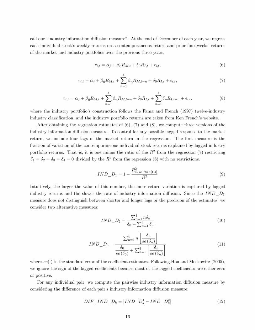
call our �industry information di¤usion measure�. At the end of December of each year, we regress

each individual stock�s weekly returns on a contemporaneous return and prior four weeks�returns

of the market and industry portfolios over the previous three years,

ri;t = �j + �0RM;t + �0RI;t + �i;t; (6)

ri;t = �j + �0RM;t +4Xn=1

�nRM;t�n + �0RI;t + �i;t; (7)

ri;t = �j + �0RM;t +4Xn=1

�nRM;t�n + �0RI;t +4Xn=1

�nRI;t�n + �i;t: (8)

where the industry portfolio�s construction follows the Fama and French (1997) twelve-industry

industry classi�cation, and the industry portfolio returns are taken from Ken French�s website.

After obtaining the regression estimates of (6), (7) and (8), we compute three versions of the

industry information di¤usion measure. To control for any possible lagged response to the market

return, we include four lags of the market return in the regression. The �rst measure is the

fraction of variation of the contemporaneous individual stock returns explained by lagged industry

portfolio returns. That is, it is one minus the ratio of the R2 from the regression (7) restricting

�1 = �2 = �3 = �4 = 0 divided by the R2 from the regression (8) with no restrictions.

IND_D1 = 1�R2�n=0;8n2[1;4]

R2(9)

Intuitively, the larger the value of this number, the more return variation is captured by lagged

industry returns and the slower the rate of industry information di¤usion. Since the IND_D1measure does not distinguish between shorter and longer lags or the precision of the estimates, we

consider two alternative measures:

IND_D2 =

P4n=1 n�n

�0 +P4n=1 �n

(10)

IND_D3 =

P4n=1 n

��n

se (�n)

��0

se (�0)+P4n=1

��n

se (�n)

� (11)

where se(�) is the standard error of the coe¢ cient estimates. Following Hou and Moskowitz (2005),we ignore the sign of the lagged coe¢ cients because most of the lagged coe¢ cients are either zero

or positive.

For any individual pair, we compute the pairwise industry information di¤usion measure by

considering the di¤erence of each pair�s industry information di¤usion measure:

DIF_IND_Dk =��IND_D1k � IND_D2k�� (12)

16

where k = 1; 2; 3 denotes the version of individual industry information di¤usion measure outlined

in (9), (10) and (11). We consider the absolute value of the di¤erence of each stock�s industry

information di¤usion measure within a pair because such di¤erence captures the di¤erence in the

lead and lag relationship with respect to the common industry level information. Since the results

from these three versions of information di¤usion measures are qualitatively similar, we choose to

focus our attention on DIF_IND_Dk=3 de�ned by (12), which is derived from IND_D3 in

(11).

Table 6 reports the results of a series of asset pricing tests for portfolios sorted on the industry

di¤usion measure given in (11) and (12). For the overall sample, as shown in Panel A, when the

di¤erence of the industry information di¤usion rates of the stocks in a pair is large, the monthly

portfolio return is about 90 basis points (bpts); and when the di¤erence is small the monthly

portfolio return is about 50 basis points. The return spreads between the large and small di¤usion

rate portfolios is about 30 basis points and statistically signi�cant at the one percent level.

Such a di¤erence is unlikely to be entirely driven by the di¤erence of pair�s average size. As

reported in Panel B and Panel C, when we �rst split the sample of pairs into two portfolios based

on pairwise average market capitalization, most of the return spreads come from large market

capitalization pairs rather than small market capitalization pairs. For example, among the large

market capitalization pairs, when the di¤erence of the industry information di¤usion rates of the

stocks in a pair is large, the monthly portfolio return is about 80 basis points (bpts); and when

the di¤erence is small, the monthly portfolio return is about 30 basis points. The return spreads

between these two portfolios are 40 basis points and statistically signi�cant at one percent level.

For the small market capitalization pairs, though as the di¤erence of information di¤usion rates for

the underlying stocks increase, monthly returns from the pairs portfolios increase as well and there

is not much spread among these portfolios. This is likely due to the fact that among small market

capitalization pairs, there is not much di¤erence in the industry information di¤usion measure. In

summary, Table 6 demonstrates that when the two stocks in the pair have large (small) di¤erences

in di¤usion rates, the pro�ts to a pairs trading strategy are also large (small). There is evidence

that when common information di¤uses into stocks at di¤erential rates, it can create the prices of

related stocks to temporarily move apart.

By taking an approach similar to Hong, Lim and Stein (2000), we consider two alternative

and indirect measures to capture the relative information di¤usion rates. Hong, Lim and Stein

(2000) test whether the slow information di¤usion model of Hong and Stein (1999) can explain the

momentum anomaly by forming portfolios based on analyst coverage. They �nd that - controlling

for �rm size - if a �rm has fewer analysts then it is more likely to experience momentum. Momentum

is a univariate strategy so that it is natural for Hong, Lim and Stein (2000) to compute the number

of analysts that cover a particular �rm; pairs trading is a bivariate strategy so that it is natural

for us to compute the number of analysts that cover both �rms. This �rst measure is called

�common analyst coverage�. For those pairs where both stocks are covered by analysts from the

same brokerage house, there should be relatively small di¤erence in information di¤usion rates. In

17

this case, the pro�ts from pairs trading should be smaller. We also construct a measure based on

common institutional holdings. For those pairs where both stocks are held by the same institutional

investors, there should be a relatively small di¤erence in information di¤usion rates. In this case,

the pro�ts from pairs trading should also be smaller.16

Table 7 and Table 8 provide evidence consistent with these hypotheses. Pairs with few common

analysts outperform pairs with many common analysts by 40 basis points per month and the spreads

are statistically signi�cant at one percent level. Similarly, pairs with few common institutional

holdings outperform pairs with more common institutional holdings by 50 basis points (bpts) per

month and such spreads are statistically signi�cant at one percent level. Splitting the sample based

on the average market capitalization of the pairs reveals that the most of the spreads between high

versus low common analyst coverage or common institutional holding portfolios come from the large

average market capitalization pairs. Large market capitalization pairs with few common analysts

outperform pairs with many common analysts by 30 basis points per month and the spreads are

statistically signi�cant at the �ve percent level. In addition, large market capitalization pairs with

few common institutional holdings outperform pairs with more common institutional holding by 20

basis points (bpts) per month and such spreads are statistically signi�cant at the ten percent level.

6 Event-Time Cross-Sectional Evidence

Thus far we have shown di¤erential pro�tability from pairs trading when we sort on liquidity, news

and information di¤usion variables in calendar-time portfolios. Here we examine these results in

event-time using cross-sectional regressions, where the unit of observation is the opening (diver-

gence) of a pair. The event-time approach has several advantages over the calendar-time approach.

First, we can run cross-sectional regressions that allows us to include a battery of control variables

so that we are more con�dent about the economic and statistical signi�cance of our main variables

of interest. In the calendar-time approach, sorting in several dimensions can create thin portfolios.

Second, the cross-sectional regressions also allow us to delineate a �ner picture of the complete

lifecycle of pairs trading: (1) the opening of the pairs (2) the evolution of the pairs along the path

of convergence, and (3) the termination of the pairs via natural or forced convergence. The analysis

required to understand this lifecycle is beyond a simple linear factor regression. Therefore, when

necessary, we introduce several econometric techniques to facilitate our analysis. We discuss these

econometric techniques and empirical results below.

6.1 Linear Regression of Pro�ts from the Pairs Trading

In Table 9 we analyze how short- and long-term pairs trading pro�ts are related to a set of pair char-

acteristics. In the calculation of standard errors, we cluster by industry, year and month, following

16An interesting question is why some pairs sometimes covered by the same brokerage (or held by the sameinstitutional investors), but some pairs are not covered by the same brokerage house (or held by the same institutionalinvestors) at some other times. This may be due to categorical thinking in the investment process as suggested byMullainathan (2000), and Barberis and Shleifer (2003).

18

Petersen (2008).17 As in section 5, we are particularly interested in how �rm-speci�c idiosyncratic

news, common information are related to the pairs trading pro�ts, and how they interact with the

underlying institutional share holding structure, information intermediary information production,

and liquidity levels.

We use a set of standard control variables, including pairwise average book-to-market equity,

the logarithm of pairwise average market capitalization, and pairwise past cumulative returns at

the horizons of one month, one year and three years. At the individual stock level, these are shown

to be related to future returns (Brennan, Chordia and Subramayahm, 1998). On average, pairs

of small stocks and growth stocks earn higher pairs trading pro�ts. Although calendar time pairs

trading pro�ts are negatively correlated to the momentum factor as shown in Table 2, we �nd little

evidence in the time-series cross-sectional regressions. The pairwise average cumulative 12-month

returns are not statistically signi�cant. Comparing Panel A and Pane B, we see that pairs with

low past one-month returns earn higher pro�ts, especially when we hold the position for up to 6

months. Consistent with the limts-to-arbitrage argument, more volatile stocks earn higher returns

in both long- and short- horizons.

Table 9 also provides evidence about how liquidity and trading volume in�uence pairs trading

pro�ts. To capture the level and change of liquidity, we introduce the pairwise average proportional

e¤ective spreads (PESPR) estimated during the portfolio formation period, and the change of pair-

wise average proportional e¤ective spreads (�PESPR) �ve trading days leading to the divergence

of the pairs. We also consider average turnover rates estimated during the portfolio formation pe-

riod, and change of average turnover rates �ve trading days leading to the divergence of the pairs.

Our results are largely consistent with the prior literature. We �nd that, depending on the return

horizons, the level and the change of turnover and proportional e¤ective spreads are related to pairs

trading pro�ts in an interesting way. With the 10-day holding restriction, the only variable that is

reliably related to the pro�ts from pairs trading is the pairwise average change of the proportional

e¤ective spreads. At the longer horizon of six months, both the pairwise average proportional

e¤ective spreads and pairwise average turnover are related to pro�ts from pairs trading. Stocks

with higher pairwise average proportional e¤ective spreads and low pairwise average turnover earn

higher pro�ts. The level of liquidity, captured by turnover and the level of spreads are related

to pro�ts from pairs trading in a longer horizon, which suggests non-information driven liquidity

demand plays an important role in explaining returns accrued to pairs trading. What is interesting

is that, at short-term, the change of liquidity level, or the liquidity shock, subsumes the level of

liquidity in explaining the returns of pairs trading. This is consistent with the model of Campbell,

Grossman and Wang (1993), which emphasize the temporary nature of liquidity demand shock and

its relation to asset prices.

We also �nd that the idiosyncratic news variable is signi�cant at both the short-term and long-

term horizons. It is statistically signi�cant at the �ve-percent level when the pairs are forced to

17We also compute the standard errors using Fama-MacBeth approach by �rst estimating a pooled regressionmonthly then average the monthly regression coe¢ cients to compute the Fama-MacBeth regression coe¢ cients. Theresults are qualitatively similar so we present the regression results clustered by year, month and industry throughout.

19

close in ten trading days and it is signi�cant at one-percent level when pairs are forced to close in

six months. In both cases, it is also economically signi�cant. On average, for the ten-day holding

horizon, pairs with news earns 40 basis points less than otherwise similar pairs; and for the six-

month holding horizon, pairs with news on one of the constituent stock earns 120 basis points less

than otherwise similar pairs. In sharp contrast, pairs with just media coverage - but not news -

do not seem to earn returns any di¤erent from stocks without any media coverage. These results

provide con�rmatory evidence that idiosyncratic news creates permanent di¤erences in the prices

of the stocks in the pair and therefore less pro�tability from a pairs trading strategy.

Fourth, the common institutional holding (Common_Holding) and the common analyst cov-

erage (Common_Analyst) measures are related to the pro�ts from pairs trading. In the second

columns of Panel A and Panel D, we consider a continuous version of these two variables as de�ned

in Section 4.2, which essentially count how many institutions hold both stocks in the pair, and how

many brokerage houses cover both stocks in the pair. In the third and fourth columns of Panel A to

Panel D, we consider binary version of these variables, which take the value of one if the number of

institutions holding both stocks in the pair is less than the sample median (about 63 institutions),

or if the number of brokerage house covering both stocks in the pair is less than the sample median

(about 2 brokerage houses). At both short and long horizons, the institutional ownership structure

of the pair matters for the pro�ts from pairs trading. Columns three in Panel A and Panel B

indicate that, compared to otherwise similar pairs, if there are few institutional investors holding

both stocks within the pair during the quarter prior to the divergence of the pair, the pairs trading

pro�ts increase about 70 to 80 basis points on average per pair. The impact of the information

intermediary structure on pairs pro�ts are weaker. If there are fewer than two brokerage houses

covering both stocks within the pair, the pro�ts from pairs trading are indeed stronger: the mag-

nitude is about 60 basis points per pair more for the longer holding horizon. However, the number

of brokerage houses covering both stocks of the pair has no impact on the pro�ts for the shorter

horizon. These results are consistent with the idea that institutions can impound information into

prices more quickly (which is why institutional ownership of the paired �rms are important for the

short-horizon) and the information produced by intermediaries like analysts takes more time to be

impounded into prices (which is why analyst coverage is important for the long-horizon).

Regressions reported in Panel C and Panel D are similar to those in Panel A and Panel B

of Table 9, except we include the industry information di¤usion measure (DIF_FF12_D3 ), and

its interactions with liquidity (Liquidity), institutional ownership structure (Common_Holding),

information intermediary structure (Common_Analyst), and size (Size) binary variables. In all

cases, the industry information di¤usion measure are statistically signi�cant. The larger the value

of the industry information di¤usion measure, the larger the di¤erence of individual stock�s speed

of response to industry common information within the pair, and the larger the pro�ts from pairs

trading. Furthermore, the interactions between industry information di¤usion measure and liquid-

ity (Liquidity), institutional ownership structure (Common_Holding), information intermediary

structure (Common_Analyst) are all statistically signi�cant at least �ve-percent signi�cance level

20

for one of the holding horizons. That is, the impact of the di¤erence of individual stock�s speed

of response to industry common information is particularly strong among less liquid stocks, stocks

with fewer common institutional holding or analyst coverage.

Finally, we point out that the interaction between pairwise average size and the industry in-

formation di¤usion measure is insigni�cant. This is consistent with our interpretation that even

though liquidity (Liquidity), institutional ownership structure (Common_Holding), information

intermediary structure (Common_Analyst) may be related to the average size of the pair, they

seem to capture something more than the size e¤ect. Moreover, they represent market frictions

in the form of transactions costs and information costs that exacerbate the di¤erential response of

paired stocks to common information which we have argue is a channel by which pro�ts are made

in pairs trading.

6.2 Logistic Regression on Pair�s Opening Probabilities

We begin our analysis of the lifecycle of pairs trading with the binary divergence event (the �open-

ing�event). This is event-day in which the pair becomes more than two standard deviations away

from the price di¤erence established in the estimation period. The logistic regression analysis on

the pair�s daily opening probability is reported in Table 10. On each day and for each pair, we

consider whether the pair remains �closed�or becomes �open�, and relate this divergence event to

a set of pair-speci�c characteristics using a logistic regression. In the calculation of standard errors,

we cluster by industry, year and month, following Petersen (2008).

As shown by the �rst regression in the Panel A of Table 10, if eligible for trading, the pair

consisting of stocks associated with higher average proportional e¤ective spreads, sudden increase

in the proportional e¤ective spreads, lower turnover rates, sudden increase in turnover rates, higher

past two-to-three year cumulative returns, lower market capitalization, lower book to market equity,

and higher idiosyncratic volatilities is more likely to open on a particularly day.

Regressions 2 to 4 in Panel A show that the common institutional holding (Common_Holding)

and the common analyst coverage (Common_Analyst) measures are related to the probability

of pair opening either individually or together. In these regressions, the common institutional

holding (Common_Holding) and the common analyst coverage (Common_Analyst) are contin-

uous variables. Serving as a robustness check, regressions 5 is similar to regression 4, but the

institutional ownership structure (Common_Holding) and the information intermediary structure

(Common_Analyst) are categorical variables. These three regressions show that the probability of

a pair opening is signi�cantly lower for those pairs with both stocks held by a larger number of the

same institutions, or covered by a large number of the same analysts.

Regressions 6 in Panel A adds another binary variable (Size_Rank) to the independent vari-

ables in regression 5, which takes the value of one if the pairwise market capitalization is lower

than the sample median. After inclusion of this variable, the magnitude and statistical signi�cance

of the institutional ownership structure (Common_Holding) and information intermediary struc-

ture (Common_Analyst) categorical variables do not change signi�cantly. Regression 7 excludes

21

the institutional ownership structure (Common_Holding) and information intermediary structure

(Common_Analyst) categorical variables from regression 6. The magnitude and statistical signi�-

cance of size (Size_Rank) categorical variable remain similar to those in regression 6. Therefore, it

is clear that the institutional ownership structure (Common_Holding) and information intermedi-

ary structure (Common_Analyst) categorical variables provide additional information beyond the

size.

In Table 10, the speci�cation of regressions 1 to 5 in Panel B is similar to regression 4 in Panel A.

The di¤erence lies in the additional industry information di¤usion measure (DIF_F12_D3 ), and

its interaction with liquidity (Liquidity), institutional ownership structure (Common_Holding), in-

formation intermediary structure (Common_Analyst), and average pairwise market capitalization

(Size_Rank). With the exception of the interaction term between the industry information di¤u-

sion measure (DIF_F12_D3 ) and the institutional ownership structure (Common_Holding), the

industry information di¤usion measure and its interaction with liquidity, information intermediary,

and average pairwise market capitalization are statistically signi�cant at one percent level. Regres-

sion 1 show the daily opening probability of the pair increases, when the di¤erence in the relative

speed of prices adjustment to industry common information of the stocks in a pair decreases (i.e.,

the larger the value of DIF_F12_D3 ). Regressions 2, 4 and 5 show the relationship between the

daily opening probability of the pair and the information di¤usion measure is stronger among the

pairs which are less liquid, covered by smaller number of the same analysts, or smaller average

pairwise market capitalization.

6.3 An Econometric Model of Time-till-Convergence

After a pair opens, we analyze its time-to convergence using survival analysis. Survival analysis

is a statistical technique developed to analyze positive-valued random variables such as life-times,

failure-times, or, in our case, the time-till-convergence. It is well suited to analyze the time it takes

for the stocks in a pair to achieve convergence because the right-censored observations (the pairs

that are forced to close because they take too long to converge naturally) can be conveniently and

accurately modelled. We discuss the survival analysis in some details in Appendix A.

Table 11 reports the survival analysis of time-till-convergence of the pairs in our sample. Several

noteworthy observations emerge. First, in all cases, the scale and shape parameter estimates are

all statistically signi�cant at one percent level, which hints that the choice of generalized gamma

distribution as the baseline distribution is preferred to some other more restrictive distribution

assumptions.

Second, pairs consisting of stocks associated with higher average proportional e¤ective spreads,

sudden increase in the proportional e¤ective spreads, lower turnover rates, sudden decrease in

turnover rates, higher past twelve-month returns, lower market capitalization, lower book to mar-

ket equity, and higher idiosyncratic volatilities have shorter times-till-convergence and, thus, less

horizon risk. On the one hand, according to the limits to arbitrage argument, it is more di¢ cult for

the rational arbitragers to arbitrage away the anomalous returns from these stocks. On the other

22

hand, they are exactly those stocks which are less liquid, smaller, and more volatile stocks. In

another word, these stocks have higher �holding risk�(Ponti¤, 2006). Thus, our survival analysis

illustrates that there is a delicate balance between the horizon risk and holding risk. Our survival

analysis clearly shows that if one is going to reduce the horizon risk; one may have to incur more

holding risk; therefore, the convergence trade is far from being risk-free in an operational sense.

To the best of our knowledge, the trade-o¤ between horizon risk and holding risk has not been

discussed in the literature.

Third, in the previous sections, we have shown that the pairs with idiosyncratic news on at least

one of the pairs at the time of divergence earns signi�cantly lower returns. Table 11 reveals that at

least part of the reason for the declines in pro�tability is the increase in the time-till-convergence.

For instance, according to the estimates from Panel A and equation (20), for a holding horizon

of ten trading days, the expected time-till-convergence for the pairs with news is about 28:40%

(= exp [0:25� (1� 0)]� 1 = 28:4%) longer than otherwise similar stocks without news (includingboth stocks without any media coverage, and the pairs with only coverage but not news); and

according to the estimates from Panel B and equation (20), for a holding horizon of six months, the

time-till-convergence for the pairs with news is about 52:20% (= exp [0:42� (1� 0)]� 1 = 52:20%)longer than otherwise similar stocks without news. Clearly, the time-till-convergence di¤erence due

to stock level idiosyncratic news is both statistically signi�cant and economically important.

Slow information di¤usion hypothesis (Hong and Stein, 1999) suggests idiosyncratic information

should cause permanent di¤erences in the arbitrage spread and may even lead to the spread widening

as the idiosyncratic information di¤uses. To test this hypothesis, we create a binary variable,

NegativeNews, which takes the value of one if on the divergence date the news associated with the

stock is negative; and zero otherwise. Then we interact the News binary variable. If the time-till-

convergence is positively related to the interaction term, News�NegativeNews, then it indicates thatdrift e¤ect is particuarly pronounced for the �bad news�pairs, and the evidence is consistent with

the �bad news�travel slowly story. In unreported regressions, we indeed �nd evidence consistent

with the hypothesis. In all speci�cations, the interaction term is staticially signi�cant at one percent

level, and all other regression coe¢ cients are qualitatively similar to those reported in Table 11.

Moreover, the point estimates for the interaction terms are about 0:27 for the holding horizon of 10

days, and 0:29 for the holding horizon of 6 months. In contrast, the point estimates for the News

variable are about 0:20 for the holding horizon of 10 days, and 0:36 for the holding horizon of 6

months. A simple back of the envelope calculation shows that the expected time-till-convergence

for the pairs with �bad news�is about 31% to 33% longer than otherwise similar stocks with �good

news�depending on the holding horizon we examine.

Fourth, the institutional ownership structure (Common_Holding) and the information inter-

mediary structure (Common_Analyst) are related to the time-till-convergence. Columns (3) and

(4) from Panel A and Panel B show that, if there are few institutions holding both stocks in a pair,

the expected time-till-convegence decreases by at least 25% (= exp [0:223� (1� 0)]�1 = 25:00%).Similarly, if there are few analysts from the same brokerage house covering both stocks of a pair,

23

the expected time-till-convegence decreases by at least 8:33% (= exp [0:08� (1� 0)]� 1 = 8:3 3%).Finally, Panel C and Panel D of Table 11 show that the larger the industry information di¤usion

measure, i.e., the larger the di¤erence between the stock�s speed of adjustment to the common

information, the shorter the expected time-till-convergence. Such e¤ect is especially strong among

small stocks, less liquid stocks, stocks with few common institutional holding, and stocks with few

common analyst coverage.

6.4 An Econometric Model of Divergence Risk

A typical arbitrager engaged in convergence trading like pairs trading faces the possible widening

of arbitrage spreads. Widening arbitrage spreads expose the arbitragers to margin calls, which may

require partial or complete liquidation of his position or additional capital infusion. In either case,

the pro�ts from convergence trading decreases. This type of arbitrage risk is commonly referred

to as �divergence risk�. For a given arbitrager, when there spreads widen, the arbitrager has the

choice of complete or partial liquidation or capital infusion; and the arbitrager also has the choice

of liquidating some assets instead of others. Without detailed assumptions on the cost of arbitrage

capital and capital constraints, it is di¢ cult to quantify directly divergence risk impact on the total

return accrued to the convergence trade. To avoid such potentially ad hoc assumptions, we choose

to model the occurrence of spread-widening events during the path of convergence trades, and traet

such occurrence as an measure of divergence risk.

For any particular pair at the end of trading day t , when the arbitrage spreads x(t) in-

crease compared with the prior maximum spreads since the establishment of the position, i.e.,

x(t) > max [x(1); x(2); :::; x (t� 1)] , we de�ne a spread-widening event occurs. Statistically, theoccurrence of spreads widening events is a set of non-negative discrete random variable. To accom-

modate the data feature, we use the zero-in�ated negative binomial regression model is a natural

candidate. A brief description of the model is presented in Appendix B, but readers interested in

a more detailed exposition should consult Cameron and Trivedi (1999).

Table 12 reports the estimates of the zero-in�ated negative binomial regression. The dependent

variable is the count of spreads-widening events during six-month holding horizon. The independent

variables in the zero-in�ation equations include a constant term, a binary indicator variable taking

value of one if the pair converges in ten days; and zero otherwise, and the change of average

pairwise proportional e¤ective spreads prior to convergence. The independent variables in the

main equations are similar to those used in the survival analysis regressions outlined in the previous

section.

To determine the model speci�cations, we tested several alternative models by including more

variables of the pairs characteristics in the auxiliary zero-in�ation equation. However, in the pres-

ence of the binary indicator variable describing whether the convergence happens in ten days or

not, most of the other variables are statistically insigni�cant at conventional level; and inclusion

of these additional variables do not signi�cantly change the estimates from the main regression, so

we choose the simpler model. The binary indicator variable describing whether the convergence

24

happens in ten days or not is always highly signi�cant in the zero-in�ation equation. Since the

divergence risk are larger for those pairs which do not converge in a relatively short period, this is

not entirely surprising.

In unreported tests, we �nd that Vuong test statistics (Vuong, 1989) indicate that the zero-

in�ated negative binomial regression model in preferred to the negative binomial regression model

against. We also �nd that the likelihood ratio test statistics reject the dispersion parameter � = 0

at one-percent signi�cance level, which indicates that the negative binomial regression model is

preferred to the Poisson regression model.

Conceptually, divergence risk and horizon risk describe di¤erent aspects of the arbitrage risks

associated with the convergence trade. For the convergence trades with �xed time-till-convergence,

i.e., no horizon risk, there still could be substantial divergence risk before the convergence (see Liu

and Longsta¤, 2006). However, divergence risk and horizon risk are not unrelated. Table 12 shows

that the divergence risk are lower among pairs with higher average proportional e¤ective spreads,

lower turnover, higher past twelve-month or three-year cumulative returns, higher idiosyncratic

volatilities, larger di¤erence in the speed of adjustment to common industry information, less

common holding by institutions, less common coverage by the sell-side analysts, and among pairs

without news. Table 12 also show that, when the stocks within the pair are less liquid, or less

likely to be held by the same institution, the speed of adjustment to common industry information

impact on the divergence risk are stronger. These results are consistent with the results from the

regressions outcome of the survival analysis reported early.

6.5 Analysis of the Speed of Convergence

The duration of time-till-convergence captures the speed of convergence in calendar days, condi-

tional on the initial divergence of the pair. However, it does not capture di¤erent initial spreads

and the speed of convergence. To see this, consider the following scenario. Both pair A and pair B

converge in twenty days. However, pair A starts with the spreads of three standard deviations away

from the historical normalized prices; while pair B starts with the spreads of �ve standard devia-

tions away from the historical normalized prices. That is, pair B starts with a much larger spreads

than pair A. Clearly, duration analysis would not have su¢ cient statistical powers to di¤erentiate

such �ties�.

To address this issue, we adopt a two-step procedure. In the �rst step, we estimate a mean-

reversion stochastic process. Speci�cally, we assume the convergence trade�s spreads follow the

familiar Ornstein-Uhlenbeck process,

dXt = �� (Xt � �) dt+ �dWt (13)

where Xt is the stochastic variable describing the convergence trade�s spreads, � > 0, � and � > 0

are constants, and Wt is the standard Wiener process. We choose Ornstein-Uhlenbeck process

not only for simplicity and tractability - given the fact that we have more than 30; 000 pairs to

25

analyze, a close-form solution is essential; but also for its wide applications in theoretical analysis

of convergence trades.18 In the second step, we regress the mean-reversion parameters against a

set of pair characteristics.

The details on the estimation of OU process, and our empirical procedure are discussed in Ap-

pendix C. The results are basically consistent with those presented in Table 11 and Table 12, thus

not reported to preserve space. Pairs trading�s speed of convergence is faster when the constituent

stocks are less liquid (higher proportional e¤ective spreads), without news coverage (News binary

variable value equals zero), higher past twelve-month cumulative returns, smaller market capitaliza-

tion, higher idiosyncratic volatilities, simultaneously held by few number of the same institutions,

and lower industry information di¤usion rates. The last e¤ect is particular strong among small,

less liquid stocks held by few number of the same institutions or covered by few analysts.

7 Robustness Check

7.1 Default Risk and Pairs Trading

We use the Expected Default Frequency (EDFTM) produced by Moody�s-KMV as a proxy for

default risk at individual stock level.19 We compute the default risk at the pair level by averaging

individual stock�s EDFs, or taking the maximum of individual stock�s EDFs within the pair. Then

we apply the pairwise EDF in the cross-sectional regressions which relate the pair�s characteristics

and pair�s total returns. As Da and Gao (2008) suggest, a sudden increase in the default likelihood

could induce a clientele change and consequently a short-term return reversal e¤ect. To avoid such

confounding e¤ect, we use the pair�s EDF value one month before the divergence month. The

regression results show that the pair�s EDF is not related to the pairs trading pro�ts for both

ten-day and six-month horizons (not reported).

7.2 Short-sale Constraints and Pairs Trading

Short-sale constraints, such as prohibitively expensive short-rebate rates, could make pairs trading

not implementable. To examine such possibility, following the identi�cation proposed by Asquith,

Pathak and Ritter (2005), Chen, Hong and Stein (2002) and Nagel (2005), we consider (i) the

minimal institutional holding of the constituents of the pair, and (ii) zero holding of institutional

holding of the constituents of the pair as proxy variables for the short-sale constraints. However,

we did not �nd either of the proxy for short-sale constraints are related to the return and risk

of pairs trading. This is likely due to the fact that the stocks in our sample are generally large

(the average market capitalization of the stocks are about 60th percentile in terms of NYSE size

percentile breakpoints), and short-sale constraints are not a major friction. For example, D�Avolio

18 In fact, almost all the papers we discussed in Section 3.2 use the Ornstein-Uhlenbeck process to model thearbitrage spreads, with the exception of Liu and Longsta¤ (2006), who apply a Brownian bridge process.

19We thank Moody�s-KMV for making the EDF TM data available to us.

26

(2002) documents that hard-to-borrow stocks almost exclusively concentrate among the smallest

size decile (based on NYSE size decile breakpoints) or low priced (less than �ve dollars).

We also consider the stocks of the pair have traded options or not. In practice, instead of

directly borrowing shares, one can construct so-called �synthetic shorts� using options (Battalio

and Schultz, 2006). Using the Ivy OptionMetric database, we �nd that more about 99:76% of the

pairs positions opened, there are options traded on the organized exchange for both stocks of the

pair.20

However, we cannot rule out the possibility that there is a short-term sudden change of short-

sale constraints but we cannot detect such short-term movement of short-sale constraints using

quarterly institutional holding data or option listing data. As short-rebate data - which could

potentially capture such sudden change of short-sale constraints - at a daily frequency is hard to

come by, we cannot directly test such possibility. We leave this lose end for future research.

8 Summary and Concluding Comments

This paper investigates the source of pro�ts from pairs trading. The following table summarizes

the main results from our empirical analysis by describing how increases in the values of certain

variables a¤ect total pairs trading pro�ts, the probability that a pair will open, the horizon risk, the

divergence risk, and the convergence speed. In this table, �+�denotes that certain variables relate

positively to trading pro�ts, the probability that a pair will open, the horizon risk, the divergence

risk, the convergence speed and arbitrage risk; ���denotes a negative relationship; and �n:s:�denotes a statistically insigni�cant relationship. Several interesting �ndings emerge.

First, when there is idiosyncratic news about at least one stock within the pair, the total pro�ts

from pairs trading decreases even though the news creates potential opportunities for pairs trading

since it is more likely that the pair may diverge. While idiosyncratic news events are more likely

to make pairs diverge, they increase the horizon risk and divergence risk to risk to the arbitrageur

and slow the speed of pair convergence.

Second, the level of liquidity and short-term changes in liquidity (�liquidity shock�) proxied by

PESPR and �PESPR contribute positively to the total pro�ts - which arises because of an increase

in opening probability, a decrease in horizon and divergence risk, and an increase in convergence

speed. However, they are also associated with increases in arbitrage risk.

Third, the di¤erence in the relative speed of adjustment to common industry information is

strongly related to pairs trading pro�ts. Large di¤erences in pairwise information di¤usion rates

contribute to the return because it creates trading opportunity, decreases the horizon risk and

divergence risk, and also increases the speed of convergence. However, these are the situations

when arbitrage risk - in particular liquidity and price impact - may be high.

Fourth, the information di¤usion rates interact with size, liquidity level, and the underlying

institutional ownership and information intermediary in a predictable way. The impact of the

20We thank Zhi Da providing us the list of stocks with traded options according to the OptionMetric database.

27

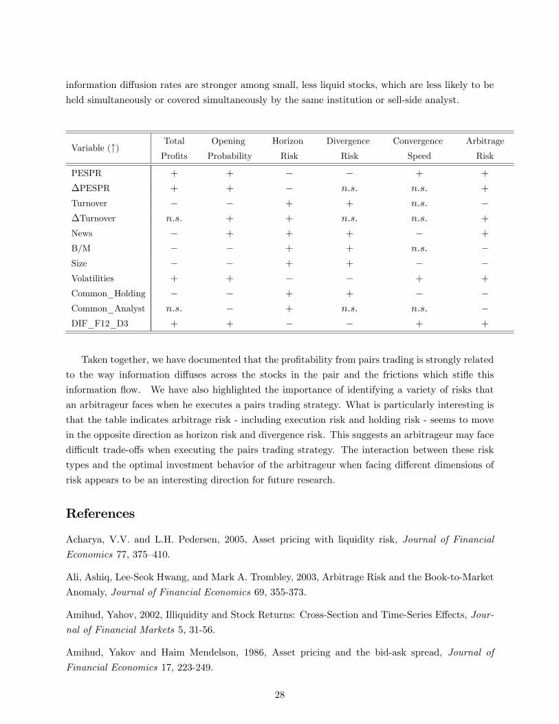
information di¤usion rates are stronger among small, less liquid stocks, which are less likely to be

held simultaneously or covered simultaneously by the same institution or sell-side analyst.

Variable (") Total

Pro�ts

Opening

Probability

Horizon

Risk

Divergence

Risk

Convergence

Speed

Arbitrage

Risk

PESPR + + � � + +

�PESPR + + � n:s: n:s: +

Turnover � � + + n:s: ��Turnover n:s: + + n:s: n:s: +

News � + + + � +

B/M � � + + n:s: �Size � � + + � �Volatilities + + � � + +

Common_Holding � � + + � �Common_Analyst n:s: � + n:s: n:s: �DIF_F12_D3 + + � � + +

Taken together, we have documented that the pro�tability from pairs trading is strongly related

to the way information di¤uses across the stocks in the pair and the frictions which sti�e this

information �ow. We have also highlighted the importance of identifying a variety of risks that

an arbitrageur faces when he executes a pairs trading strategy. What is particularly interesting is

that the table indicates arbitrage risk - including execution risk and holding risk - seems to move

in the opposite direction as horizon risk and divergence risk. This suggests an arbitrageur may face

di¢ cult trade-o¤s when executing the pairs trading strategy. The interaction between these risk

types and the optimal investment behavior of the arbitrageur when facing di¤erent dimensions of

risk appears to be an interesting direction for future research.

References

Acharya, V.V. and L.H. Pedersen, 2005, Asset pricing with liquidity risk, Journal of Financial

Economics 77, 375�410.

Ali, Ashiq, Lee-Seok Hwang, and Mark A. Trombley, 2003, Arbitrage Risk and the Book-to-Market

Anomaly, Journal of Financial Economics 69, 355-373.

Amihud, Yahov, 2002, Illiquidity and Stock Returns: Cross-Section and Time-Series E¤ects, Jour-

nal of Financial Markets 5, 31-56.

Amihud, Yakov and Haim Mendelson, 1986, Asset pricing and the bid-ask spread, Journal of

Financial Economics 17, 223-249.

28

Antweiler, Werner, and Murray Z. Frank, 2004, The market impact of corporate news stories,

Working Paper, Carlson School of Management, University of Minnesota.

Asness Cli¤ord S., Tobias J. Moskowitz, and Lasse H. Pedersen, 2008, Value and Momentum

Everywhere, Working Paper, AQR Asset Management.

Asquith, Paul, Parag A. Pathak and Jay R. Ritter, 2005, Short interest, institutional ownership,

and stock returns, Journal of Financial Economics 78, 243-276.

Avramov, Doron, Tarun Chordia and Amit Goyal, 2005, Liquidity and autocorrelations in individ-

ual stock returns, Journal of Finance 61, 2365-2394.

Avramov, Doron, Tarun Chordia and Amit Goyal, 2006, The Impact of Trades on Daily Volatility,

Review of Financial Studies 19, 1241-1277.

Andrade, S., Di Pietro, V., Seasholes, M., 2005, Understanding the pro�tability of pairs trading,

Working Paper, Northwestern University.

Ball, Ray, and Philip Brown, 1968, An Empirical Evaluation of Accounting Income Numbers,

Journal of Accounting Research 6, 159-178.

Barberis, Nicholas, and Andrei Shleifer, 2003, Style Investing, Journal of Financial Economics 68,

161-199.

Battalio Robert H., and Richard R. Mendenhall, 2007, Post-Earnings Announcement Drift: Timing

and Liquidity Costs, Working Paper, University of Notre Dame.

Battalio Robert H., and Paul Schultz, 2006, Options and Bubble, Journal of Finance 61, 2071 -

2102.

Berk, Jonathan, Richard Green, and Vasant Naik, 1999, Optimal Investment, Growth Options and

Security Returns, Journal of Finance 54, 1153-1607.

Bernard, V.L., Thomas, J.K., 1989, Post-earnings announcement drift: delayed price response or

risk premium?, Journal of Accounting Research 27, 1�36.

Bessembinder, Hendrik, 2003, Issues in Assessing Trade Execution Costs, Journal of Financial

Markets 6, 233-257.

Bossaerts, Peter, 1988, Common Nonstationary Components of Asset Prices, Journal of Economic

Dynamics and Control 12, 347-364.

Brennan, Michael J., Tarun Chordia, and Avanidhar Subrahmanyam, 1998, Alternative Factor

Speci�cations, Security Characteristics, and the Cross-Section of Expected Stock Returns, Journal

of Financial Economics 49, 345-373.

29

Brunnermeier, Markus K., and Lasse Heje Pedersen, 2008, Market Liquidity and Funding Liquidity,

Review of Financial Studies, Forthcoming.

Brunnermeier, Markus K., Stefan Nagel, and Lasse Heje Pedersen, 2008, Carry Trades and Currency

Crashes, NBER Macro Annual, Forthcoming.

Campbell, J. Y., S. J. Grossman, and J. Wang, 1993, Trading volume and serial correlation in stock

returns, Quarterly Journal of Economics 108, 905�939.

Carhart, Mark M., 1997, On persistence in mutual fund performance, Journal of Finance 52, 57�82.

Cameron, A. Colin, and Pravin K. Trivedi, 1998, Regression Analysis of Count Data (Econometric

Society Mongraphs), Cambridge University Press.

Chan, Wesley S., 2003, Stock price reaction to news and no-news: drift and reversal after headlines,

Journal of Financial Economics 70, 223-260.

Chen, Joseph, Harrison Hong and Jeremy C. Stein, 2002, Breadth of ownership and stock returns,

Journal of Financial Economics 66, 171-205.

Chordia, Tarun, Sahn-Wook Huh, and Avanidhar Subrahmanyam, 2007, The cross-section of ex-

pected trading activity, Review of Financial Studies 20, 709-740.

Chordia, Tarun and Avanidhar Subrahmanyam, 2004, Order imbalance and individual stock re-

turns: Theory and evidence, Journal of Financial Economics 72, 485 - 518.

Chordia, Tarun, and Bhaskaran Swaminathan, 2000, Trading Volume and Cross-Autocorrelations

in Stock Returns, The Journal of Finance 55, 913-935.

Christie, William C., Shane A. Corwin, and Je¤rey H. Harris, 2002, Nasdaq Trading Halts: The

impact of market mechanisms on prices, trading activity, and execution costs, Journal of Finance

57, 2002.

Cohen, Lauren, and Andrea Frazzini, 2008, Economic Links and Predictable Returns, Journal of

Finance 63, 1977 - 2011.

Conrad, J. S., A. Hameed and C. Niden, 1994, Volume and autocovariances in short-horizon indi-

vidual security returns, Journal of Finance 49, 1305-1329.

1999, Filter Rules Based on Price and Volume in Individual Security Overreaction, The Review of

Financial Studies 12, 901-935.

Corwin, Shane A., and Marc L. Lipson, 2000, Order �ows and liquidity around NYSE trading halts,

Journal of Finance 55, 1771-1801.

Cox, D.R., and David Oakes, 1984, Analysis of Survival Data, Chapman & Hall, New York.

30

Da, Zhi and Pengjie Gao, 2008, Clientele Change, Liquidity shock, and the Return on Financially

Distressed Stocks, Journal of Financial and Quantitative Analysis, Forthcoming.

Daniel, Kent, Mark Grinblatt, Sheridan Titman, and Russ Wermers, 1997, Measuring mutual fund

performance with characteristic based benchmarks, Journal of Finance 52, 1035�1058.

D�Avolio, Gene, 2002, The market for borrowing stock, Journal of Financial Economics 66, 271-

306.

D�Avolio, Gene Michael, 2003, Essays in �nancial economics, unpublished Ph.D. dissertation, Har-

vard University.

De Long, J. Bradford, Andrei Shleifer, Lawrence H. Summers, and Robert J. Waldman, 1990, Noise

Trader Risk in Financial Markets, Journal of Political Economy.

Elliott, Robert J., John Van Der Hoek and William P. Malcolm, 2005, Pairs Trading, Quantitative

Finance 5, 271-276.

Fama, Eugene F., Kenneth R. French, 1993. Common risk factors in the returns on stocks and

bonds, Journal of Financial Economics 33, 3-56.

Fama, Eugene F., Kenneth R. French, 1996. Multifactor explanations of asset pricing anomalies,

Journal of Finance 51, 55-84.

Fama, Eugene, Kenneth French, 1997, Industry costs of equity, Journal of Financial Economics

43, 153�193.

Fama, Eugene F., and James D. MacBeth, 1973, Risk, Return, and Equilibrium: Empirical Tests,

The Journal of Political Economy 81, 607-636.

Fang, Lily H., and Joel Peress, 2008, Media Coverage and the Cross-Section of Stock Returns,

Working Paper, INSEAD.

Gatev, Evan, William N. Goetzmann, and K. Geert Rouwenhorst, 2006, Pairs Trading: Performance

of a Relative-Value Arbitrage, Review of Financial Studies 19, 797 - 827.

Gervais, Simon, Ron Kaniel and Dan H. Mingelgrin, 2001, The High-Volume Return Premium, The

Journal of Finance 56, 877-919.

Gourieroux, Christian and Joann Jasiak, 2001, Financial Econometrics: Problems, Models, and

Methods, Princeton University Press.

Grossman, S., and J. Stiglitz, 1980, On the impossibility of informational e¢ cient markets, Amer-

ican Economic Review 70, 393-408.

Hanna, J. D., and Mark J. Ready, 2005, Pro�table Predictability in the Cross Section of Stock

Returns, Journal of Financial Economics, 78, 463-505.

31

Harris, Larry, 2002, Trading and Exchanges: Market Microstructure for Practitioners, Oxford

University Press.

Haugen, Robert A., and Nardin L. Baker, 1996, Commonality in the Determinants of Expected

Stock Returns, Journal of Financial Economics, 41, 401-439.

Hong, Harrison, and Jeremy C. Stein, 1999, A uni�ed theory of underreaction, momentum trading,

and overreaction in asset markets, Journal of Finance, Vol 54, 2143-2184.

Hong, Harrison, Terrance Lim, and Jeremy C. Stein, 2000, Bad news travels slowly: Size, analyst

coverage, and the pro�tability of momentum strategies, Journal of Finance 55, 265-295.

Hong, Harrison, Walter Torous and Rossen Valkanov, 2007, Do industries lead stock markets?,

Journal of Financial Economics 83, 367-396.

Hou, K., 2006, Industry information di¤usion and the lead-lag e¤ect in stock returns, Review of

Financial Studies 20, 1113-1138.

Hou, K., Moskowitz, T., 2005. Market frictions, price delay, and the cross-section of expected

returns, Review of Financial Studies 18, 981-1020.

Huang, Roger. and Hans R. Stoll, 1996, Dealer versus Auction markets: a paired comparison of

execution costs on Nasdaq and the NYSE, Journal of Financial Economics 41, 313-358.

Ikenberry, David, Josef Lakonishok, and Theo Vermaelen, 1995, Market underreaction to open

market share repurchases, Journal of Financial Economics 39, 181-208.

Jegadeesh, Narasimhan, and Sheridan Titman, 2001, Pro�tability of Momentum Strategies: An

Evaluation of Alternative Explanations, The Journal of Finance 56, 699-720.

Jegadeesh, Narasimhan, and Sheridan Titman, 2001, Pro�tability of momentum strategies: An

evaluation of alternative explanations, Journal of Finance 56, 699-720.

Jurek, Jakub W., and Halla Yang, 2005, Dynamic Portfolio Selection in Arbitrage,Working Paper,

Harvard University.

Kalb�eisch, J. D., and R. L. Prentice, 2002, The statistical analysis of failure time data, 2nd edition,

New York, Wiley.

Kavajecz, Kenneth A. and Elizabeth Odders-White, 2004, Technical Analysis and Liquidity Provi-

sion, Review of Financial Studies 17, 1043-1071.

Korajczyk, Rorbert A. and Ronnie Sadka, 2004, Are momentum pro�ts robust to trading costs?,

Journal of Finance 59, 1039�1082.

Kondor, Peter, 2008, Risk in Dynamic Arbitrage: The Price E¤ects of Convergence, Journal of

Finance, Forthcoming.

32

Krishnamurthy, Arvind, and Annette Vissing-Jorgensen, 2008, The aggregate demand for treasury

debt, Working Paper, Northwestern University.

Lee, Charles M. C., and Mark J. Ready, 1991, Inferring trade direction from intraday data, Journal

of Finance 46, 733-746.

Lee, Charles M. C., Mark J. Ready, and Paul J. Seguin, 1994, Volume, volatility, and New York

Stock Exchange trading halts, Journal of Finance 49, 183-214.

Lehmann, Bruce, 1990, Fads, Martingales and Market E¢ ciency, Quarterly Journal of Economics

105, 1�28.

Lesmond, David A., Michael J. Schill and Chunsheng Zhou, 2004, The illusory nature of momentum

pro�ts, Journal of Financial Economics 71, 349�380

Liu, Jun and Francis A. Longsta¤, 2004, Losing Money on Arbitrage: Optimal Dynamic Portfolio

Choices in Markets with Arbitrage Opportunities, Review of Financial Studies 17, 611-641.

Llorente, Guillermo, Roni Michaely, Gideon Saar, and Jiang Wang, 2002, Dynamic volume-return

relation of individual stocks, Review of Financial Studies 15, 1005 - 1047.

Lo, Andrew W., Craig MacKinlay and June Zhang, 2002, Econometric models of limit-order exe-

cutions, Journal of Financial Economics 65, 31 - 71.

Lo, AW, and AC MacKinlay, 1990, When are Contrarian Pro�ts due to Stock Market Overreaction?

Review of Financial Studies 3, 175-205.

Loughran, Tim, and Jay Ritter, 1997, The Operating Performance of Firms Conducting Seasoned

Equity O¤erings, Journal of Finance 52, 1823-1850.

Loughran, Tim, and Jay Ritter, 1995, The new issue puzzle, Journal of Finance 50, 23 - 51.

Mech, Timothy S., 1993, Portfolio Return Autocorrelation, Journal of Financial Economics 34,

307-344.

Mendenhall, Richard R., 2004, Arbitrage risk and post-earnings-announcement drift, Journal of

Business 77, 875�894.

Menzly, Lior and Oguzhan Ozbas, 2006, Cross-Industry Momentum, Working Paper, Marshall

School of Business, University of Southern Carlifornia.

Michaely, Roni, Richard H. Thaler, and Kent Womack, 1995, Price Reactions to Dividend Initia-

tions and Omissions: Overreaction or Drift?, Journal of Finance 50, 573�608.

Mitchell, Mark, Todd Pulvino, and Erik Sta¤ord, 2002, Limited Arbitrage in Equity Markets, The

Journal of Finance 57, 551-584.

33

Mitchell, Mark, and Todd Pulvino, 2001, Characteristics of Risk and Return in Risk Arbitrage,

The Journal of Finance 56, 2135-2175.

Mullainathan, Sendhil, 2000, Thinking through Categories, Working Paper, Harvard University.

Nagel, Stefan, 2005, Short sales, institutional investors and the cross-section of stock returns,

Journal of Financial Economics 78, 277-309.

Pástor, �Lubo�, and Robert F. Stambaugh, 2003, Liquidity risk and expected stock returns, Journal

of Political Economy 111, 642-685.

Petersen, Mitchell A., 2008, Estimating Standard Errors in Finance Panel Data Sets: Comparing

Approaches, Review of Financial Studies, forthcoming.

Ponti¤, Je¤rey, 2006, Costly Arbitrage and the Myth of Idiosyncratic Risk, Journal of Accounting

and Economics, 42, 35-52.

Ponti¤, Je¤rey, 1996, Costly Arbitrage: Evidence from Closed-End Funds, The Quarterly Journal

of Economics 111, 1135-1151.

Protter, Philip E., 2005, Stochastic Integration and Di¤erential Equations, 2nd Edition, Springer.

Ready, Mark J., 2002, Pro�ts from Technical Trading Rules, Financial Management 31, 43-61.

Sadka, Ronnie, 2006, Momentum and post-earnings-announcement drift anomalies: The role of

liquidity risk, Journal of Financial Economics 80,309-349.

Shleifer, Andrei, and Robert W. Vishny, 1997, The limits of arbitrage, Journal of Finance 52,

35-55.

Schultz, Paul, and Sophie Shive, 2008, Where are the limits to arbitrage? An application to dual-

class shares, Working Paper, University of Notre Dame

Smith, Brain F. and Ben Amoako-Adu, 1995, Relative Prices of Dual Class Shares, Journal of

Financial and Quantitative Analysis 30, 223-239.

Tetlock, Paul C., All the News That�s Fit to Reprint: Do Investors React to Stale Information?,

Working Paper, Columbia Business School.

Tetlock, Paul C., 2007, Giving content to investor sentiment: the role of media in the stock market,

Journal of Finance 62, 1139-1168.

Vega, Clara, 2006, Stock price reaction to Public and private information, Journal of Financial

Economics 82, 103-133.

Wurgler, J. and K. Zhuravskaya, 2002, Does arbitrage �atten demand curves for stocks?, Journal

of Business 75, 583-608.

34

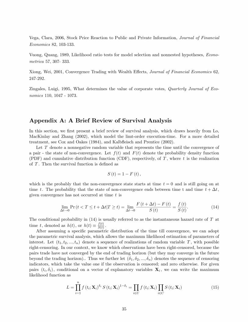
Vega, Clara, 2006, Stock Price Reaction to Public and Private Information, Journal of Financial

Economics 82, 103-133.

Vuong, Quang, 1989, Likelihood ratio tests for model selection and nonnested hypotheses, Econo-

metrica 57, 307- 333.

Xiong, Wei, 2001, Convergence Trading with Wealth E¤ects, Journal of Financial Economics 62,

247-292.

Zingales, Luigi, 1995, What determines the value of corporate votes, Quarterly Journal of Eco-

nomics 110, 1047 - 1073.

Appendix A: A Brief Review of Survival Analysis

In this section, we �rst present a brief review of survival analysis, which draws heavily from Lo,MacKinlay and Zhang (2002), which model the limt-order execution-time. For a more detailedtreatment, see Cox and Oakes (1984), and Kalb�eisch and Prentice (2002).

Let T denote a nonnegative random variable that represents the time until the convergence ofa pair - the state of non-convergence. Let f(t) and F (t) denote the probability density function(PDF) and cumulative distribution function (CDF), respectively, of T , where t is the realizationof T . Then the survival function is de�ned as

S (t) = 1� F (t) ;

which is the probably that the non-convergence state starts at time t = 0 and is still going on attime t . The probability that the state of non-convergence ends between time t and time t+�t ,given convergence has not occurred at time t is

lim�t!0

Pr (t < T � t+�tjT � t) = lim�t!0

F (t+�t)� F (t)S (t)

=f (t)

S (t): (14)

The conditional probability in (14) is usually referred to as the instantaneous hazard rate of T attime t , denoted as h(t) , or h(t) � f(t)

S(t) .After assuming a speci�c parametric distribution of the time till convergence, we can adopt

the parametric survival analysis, which allows the maximum likelihood estimation of parameters ofinterest. Let (t1; t2; :::; tn) denote a sequence of realizations of random variable T , with possibleright-censoring. In our context, we know which observations have been right-censored, because thepairs trade have not converged by the end of trading horizon (but they may converge in the futurebeyond the trading horizon).. Thus we further let (�1; �2; :::; �n) denotes the sequence of censoringindicators, which take the value one if the observation is censored; and zero otherwise. For givenpairs (ti; �i) , conditional on a vector of explanatory variables Xi , we can write the maximumlikelihood function as

L =nYi=1

f (ti;Xi)�i S (ti;Xi)

1��i =Yi2U

f (ti;Xi)Yi2C

S (ti;Xi) (15)

35

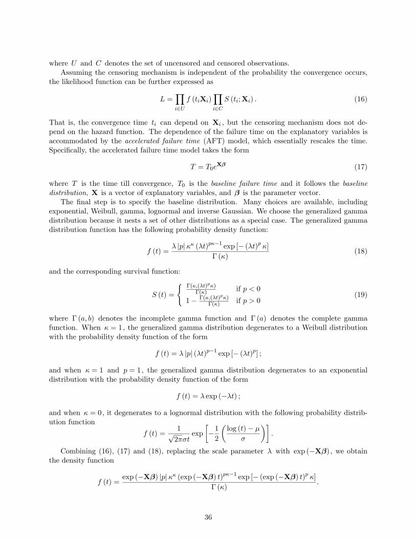
where U and C denotes the set of uncensored and censored observations.Assuming the censoring mechanism is independent of the probability the convergence occurs,

the likelihood function can be further expressed as

L =Yi2U

f (tiXi)Yi2C

S (ti;Xi) : (16)

That is, the convergence time ti can depend on Xi , but the censoring mechanism does not de-pend on the hazard function. The dependence of the failure time on the explanatory variables isaccommodated by the accelerated failure time (AFT) model, which essentially rescales the time.Speci�cally, the accelerated failure time model takes the form

T = T0eX� (17)

where T is the time till convergence, T0 is the baseline failure time and it follows the baselinedistribution, X is a vector of explanatory variables, and � is the parameter vector.

The �nal step is to specify the baseline distribution. Many choices are available, includingexponential, Weibull, gamma, lognormal and inverse Gaussian. We choose the generalized gammadistribution because it nests a set of other distributions as a special case. The generalized gammadistribution function has the following probability density function:

f (t) =� jpj�� (�t)p��1 exp [� (�t)p �]

� (�)(18)

and the corresponding survival function:

S (t) =

(�(�;(�t)p�)

�(�) if p < 0

1� �(�;(�t)p�)�(�) if p > 0

(19)

where � (a; b) denotes the incomplete gamma function and � (a) denotes the complete gammafunction. When � = 1 , the generalized gamma distribution degenerates to a Weibull distributionwith the probability density function of the form

f (t) = � jpj (�t)p�1 exp [� (�t)p] ;

and when � = 1 and p = 1 , the generalized gamma distribution degenerates to an exponentialdistribution with the probability density function of the form

f (t) = � exp (��t) ;

and when � = 0 , it degenerates to a lognormal distribution with the following probability distrib-ution function

f (t) =1p2��t

exp

��12

�log (t)� �

�

��:

Combining (16), (17) and (18), replacing the scale parameter � with exp (�X�) , we obtainthe density function

f (t) =exp (�X�) jpj�� (exp (�X�) t)p��1 exp [� (exp (�X�) t)p �]

� (�):

36

It is easy to see that the accelerated failure time (AFT) model assumes that the e¤ect of explanatoryvariables on the time till convergence is to rescale the failure time itself. The sign and estimatesof the coe¢ cient of an individual variable indicate the direction and magnitude of the partiale¤ect of the variable on the conditional probability of pairs convergence. Finally, the conditionalexpectation of failure time is exponential-linear in the product term of covariates and coe¢ cients.Thus, the ratio of the conditional expectations based on di¤erent realizations of the covariates canbe expressed as

E[T jX1]=E [T jX2] = exph(X1 �X2)T �

i; (20)

which will be used in interpreting some of the later results.

Appendix B: A Brief Review of Event Count Model

Assume a discrete random variable Y - in our application, it is the number of times the pair�sspread widens compared to previous maximum spread - follows the negative binomial distribution,then its probability distribution function can be written as

Pr (Y = y) � NB (�; u) =��y + ��1

�y!� (��1)

���1

��1 + u

���1 ���1

��1 + u

�y; y = 0; 1; 2; ::: (21)

where � (:) is the Gamma probability distribution, � is the dispersion parameter. As the dispersionparameter � increases, the variance of the negative binomial distribution also increases; and as thedispersion parameter � decreases to zero, the negative binomial distribution degenerates to thefamiliar Poisson distribution. One can test whether the data come from the Poisson process or thenegative binomial process using a likelihood ratio test. The negative binomial regression modelincorporates the observed and unobserved heterogeneity into conditional mean via an exponentialmean function

ui (�) � exp (Xi�+�i) (22)

which makes use of the linear index function Xi� to take into account the observed heterogeneityand �i to take into account the unobserved heterogeneity. If one has reasons to believe the excessiveamount of zeros of the distribution results from a di¤erent data generating process, the negativebinomial distribution regression model can be modi�ed into so-called �zero-in�ated�negative bi-nomial regression, which allows one to model each of the data generating processes separately.Speci�cally, the zero-in�ated negative binomial regression take the following form

y =

�0 with probability qNB (�; u) with probability (1� q) (23)

where the probability q is described as a logistic distribution function

qi = �i (�) =exp (Zi�)

1 + exp (Zi�)(24)

where Zi is the set of attributes which may or may not overlap the set of attributes Xi . AVuong test (Vuong, 1989) can be applied to test the negative binomial regression model againstthe zero-in�ated negative binomial regression model.

37

Appendix C: A Brief Review of Ornstein-Uhlenbeck Process

To estimate the mean-reversion parameter values, we �rst consider the transition density functionof the Ornstein-Uhlenbeck process. The Ornstein-Uhlenbeck process has the following transitiondensity function (Protter, 2005),

f (Xt = x) =1p

2�s (t)exp

"�(x�m (t))

2

2s2 (t)

#(25)

wherem (t) = �� (xt � �) exp [�� (t� t0)]

and

s (t) =�2

2�f1� exp [�2� (t� t0)]g :

It is clear that as t! +1 , m (t)! � and s (t)! �2

2�. Now we apply the discrete version of

the model to �t the data, and recover the parameters from the underlying continuous process. Itturns out that, as �t! 0 , the following process approaches the Ornstein-Uhlenbeck process in(13) (Gourieroux and Jasiak, 2001)

xt � xt�1 = � (1� exp (��)) + (exp (��)� 1)xt�1 + �t (26)

where the residual follows the following zero-mean normal distribution

�t � N 0;

�1� exp (�2�) �

2

2�

�2!:

Since we are interested in obtaining a consistent estimate of �, we estimate the following re-gression model,

xt � xt�1 = A+Bxt�1 + �t (27)

where A = � (1� exp (��)) and B = (exp (��)� 1) . After obtaining the estimates of A and B,we uncover the parameters describing the Ornstein-Uhlenbeck process:

� = �AB

� = � log (1 +B)

� = ��

�log (1 +B)

(1 +B)2 � 1

� 12

which would be used in the second step cross-sectional analysis.To estimate the mean reversion parameter, we �rst normalize the arbitrage spread for each

pair at the time of divergence to be one. The daily arbitrage spreads during the holding period isproportional to the normalized divergence date arbitrage spread. This normalization ensures ourestimates are comparable cross pairs. We discard all estimates where the estimated mean reversionparameter values are missing due to non-convergence of the �rst stage estimation, or non-positivedue to the constraint imposed by the Ornstein-Uhlenbeck process. The caveat is that there couldbe a sample selection issue. The sample selection could arise because of very �fast convergences�pairs, i.e., pairs converge in three days or less and we can not obtain the estimates of mean

38

reversion parameter. The sample selection could also arise because of very �slow convergences�pairs, i.e., pairs do not converge but diverge, which makes the mean reversion parameter valuenegative and large in absolute values. Therefore, one should bear in mind the issue of self-selectionwhen interpreting the following results, and view them in conjunction with those discussed in thehorizon risk and divergence risk. These estimates speak better for the pairs where the convergenceis neither too fast nor too slow.21

Appendix D: Alternative Factor Models

Equity Market Liquidity Risk Several recent theoretical papers consider how returns to conver-gence trading is related to market liquidity. For instance, Kondo (2008) suggests that liquidity risk(Pastor and Stambaugh, 2003; Acharya and Pedersen, 2005) is related to the arbitrageur�s pro�ts,which have a left-skewed distribution. Kondo�s model is also related to funding liquidity and themarket liquidity channel in Brunnermeier and Pedersen (2008), which underscores the importanceof funding liquidity risk.

Table A.1 in the appendix consider several alternative factor models with di¤erent equity marketliquidity factors. Panel A considers the pairs trading with a holding horizon of ten days; and PanelB considers the pairs trading with a holding horizon of six months. In the columns (1) and (2) ofeach panel, the liquidity factors are respectively the value-weighted version and equally-weightedversion of Pastor-Stambaugh liquidity factor (Pastor and Stambaugh, 2003). In columns (3) and (4)of each panel, the liquidity factors are the �xed-cost and variable-cost components of the spreadsliquidity constructed by Sadka (2006). Due to availability of liquidity risk factors, the sample periodfor regressions (1) and (2) is from January, 1993 to December, 2004; and the sample period forregressions (3) and (4) is from January, 1993 to December, 2005. The equally weighted version ofthe liquidity factors in Pastor and Stambaugh (2003), and the liquidity risk factor from the variable-costs component of total spreads in Sadka (2006) are negatively correlated with the returns frompairs trading, especially when the holding horizon is relatively short such as ten days. The abilityof these factors to explain the returns in the time-series regressions is limited though, especiallyfor short holding horizon. The R-squared from these regression are usually quite low, especiallyfor ten day holding horizon - about 6 to 9%; but increases to about 30% for holding horizon of sixmonths. The alphas of pairs trading (the intercept terms of these regressions) hardly change withthese additional liquidity risk factors.

Funding Liquidity Risk and Other Macro Risks Brunnermeier, Nagel and Pedersen(2008), and Asness, Moskowitz and Pedersen (2008) show foreign exchange carry trades andvalue/momentum strategy returns are related to funding liquidity risk. To explore the pairs tradingexposure to this macro liquidity risk, we adopt a funding liquidity risk proxy, the U.S. Treasury-Eurodollar (TED) spreads proposed by these authors. Krishnamurthy and Vissing-Jorgensen (2008)suggest the AAA/T-bill spreads capture the convenience yields of the U.S. treasury securities tothe investors. We adopt the AAA/T-bill spreads to proxy for the demand-side driven liquiditypremium in the economy. To link the pro�ts from pairs trading to the long-run consumption risk(Bansal and Yaron, 2004; Parker and Julliard, 2005; Malloy, Moskowitz and Vissing-Jorgensen,2007; Jagannathan and Wang, 2007). To capture the business cycle risk, we use default spreads,which is computed as the Moody�s BAA minus AAA bond yield spreads (Fama and French, 1999;Jagannathan and Wang, 1996; among others).

To construct US Treasury-Eurodollar (TED) spreads (Asness, Moskowitz and Pedersen. 2008),

21To address this potential sample selection problem, we estimate a version of self-selection model. The signs andmagnitudes of the parameter estimates are largely consistent with the simple regression we discuss below.

39

we obtain the 3-month LIBOR rate (in US$) from the ECONSTATS database, and 3-month Trea-sury Bill rates from Federal Reserve Board H15 release. We also obtain the Moody�s BAA,and Moody�s AAA corporate bond rates from Federal Reserve Board H15 release to constructBAA/AAA spreads and AAA/T-Bill spreads. In the construction of the long-run consumptiongrowth rates, per capital real nondurable goods quarterly consumption are derived from Table 2.1(line 6, real nondurable goods quarterly consumption) and Table 2.3.6 (line 38, population) Na-tional Income and Product Account (NIPA) database. Long-run consumption growth is the futurethree-year growth in consumption, measured as the sum of log quarterly consumption growth fromquarter q to q + 12 (both inclusive).22

The results are reported in Table A.2. In general, the exposures of pairs trading to long-run con-sumption growth, AAA/T-bill spreads and default spreads are low and statistically insigni�cant.However, the exposure to the U.S. Treasury-Eurodollar (TED) spreads is high and statisticallysigni�cant. This is the case for the strategy with a holding period of up to ten days or up tosix months. These results suggest that although pairs trading may have little exposure to macro-economic risk factors, its exposure to the funding liquidity risk is large. When the TED spreadsare wide, borrowing is di¢ cult. At the same time, the returns from the pairs trading are high.One interpretation of the relationship is that arbitragers who are enforcing the relative pricing ofstocks within the pair are constrained to participate in the market, which leaves the relatively widespreads.

Taken together, the macro risk factors, particular the macro liquidity risk, could explain someof the pro�ts from the pairs trading. However, a large fraction of the returns accrued to pairstrading is left unexplained as shown by a low R-squared of 6:6 � 10:3%.

22LIBOR rates can be accessed from the following website: http://www.econstats.com/r/rlib__d1.htm; FederalReserve H15 release can be access from the following website: http://www.federalreserve.gov/releases/h15/data.htm;and NIPA data can be accessed from the following website: http://www.bea.gov/bea/dn/nipaweb

40

41

Figure 1. Pairs Trading Profitability in Event Time

The lines plots mean returns in event time from a pairs trading strategy. The pairs trading strategy involves matching stock pairs

based on normalized price difference over a one year estimation period. Then, during the following year, the strategy looks for

instances in which the price of the two stocks in the pair diverge by more than two standard deviations of the price difference

established during the estimation period. This is called divergence (convergence is the event when, after divergence, the pairs

have no difference in normalized price). When there is divergence the strategy buys the stock that went up and shorts the stock

that went down. Event day 0 is one day after this divergence and is meant to control for bid-ask bounce. The dashed line plots

the mean return in event time from a pairs trading strategy and the solid line plots the corresponding 5 day moving average.

0

5

10

15

20

25

1 3 5 7 9

11

13

15

17

19

21

23

25

27

29

31

33

35

37

39

41

43

45

47

49

Event Day

Profitability (in Basis Points)

5 Day Moving Average

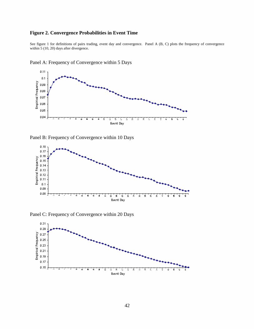
42

Figure 2. Convergence Probabilities in Event Time

See figure 1 for definitions of pairs trading, event day and convergence. Panel A (B, C) plots the frequency of convergence

within 5 (10, 20) days after divergence.

Panel A: Frequency of Convergence within 5 Days

Panel B: Frequency of Convergence within 10 Days

Panel C: Frequency of Convergence within 20 Days

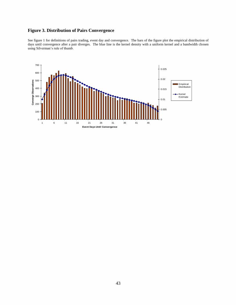
43

Figure 3. Distribution of Pairs Convergence

See figure 1 for definitions of pairs trading, event day and convergence. The bars of the figure plot the empirical distribution of

days until convergence after a pair diverges. The blue line is the kernel density with a uniform kernel and a bandwidth chosen

using Silverman’s rule of thumb.

0

100

200

300

400

500

600

700

1 6 11 16 21 26 31 36 41 46

Event Days Until Convergence

Co

nverg

e O

bserv

ati

on

s

0

0.005

0.01

0.015

0.02

0.025

Empirical

Distribution

Kernel

Estimate

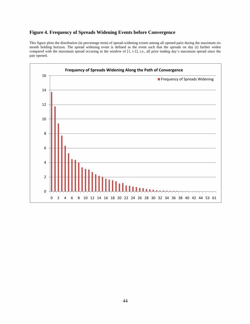
44

Figure 4. Frequency of Spreads Widening Events before Convergence

This figure plots the distribution (in percentage term) of spread-widening events among all opened pairs during the maximum six

month holding horizon. The spread widening event is defined as the event such that the spreads on day (t) further widen

compared with the maximum spread occuring in the window of [1, t-1], i.e., all prior trading day’s maximum spread since the

pair opened.

0

2

4

6

8

10

12

14

16

0 2 4 6 8 10 12 14 16 18 20 22 24 26 28 30 32 34 36 38 40 42 44 53 61

Frequency of Spreads Widening Along the Path of Convergence

Frequency of Spreads Widening

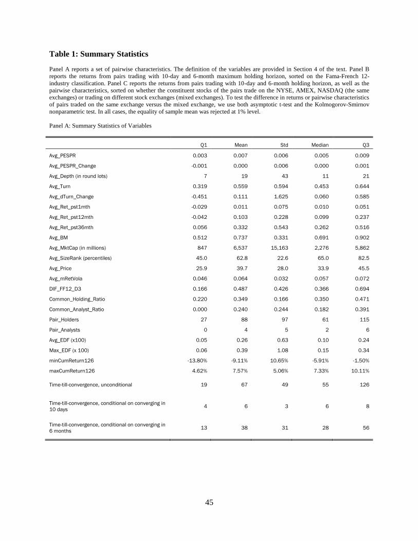
45

Table 1: Summary Statistics

Panel A reports a set of pairwise characteristics. The definition of the variables are provided in Section 4 of the text. Panel B

reports the returns from pairs trading with 10-day and 6-month maximum holding horizon, sorted on the Fama-French 12-

industry classification. Panel C reports the returns from pairs trading with 10-day and 6-month holding horizon, as well as the

pairwise characteristics, sorted on whether the constituent stocks of the pairs trade on the NYSE, AMEX, NASDAQ (the same

exchanges) or trading on different stock exchanges (mixed exchanges). To test the difference in returns or pairwise characteristics

of pairs traded on the same exchange versus the mixed exchange, we use both asymptotic t-test and the Kolmogorov-Smirnov

nonparametric test. In all cases, the equality of sample mean was rejected at 1% level.

Panel A: Summary Statistics of Variables

Q1 Mean Std Median Q3

Avg_PESPR 0.003 0.007 0.006 0.005 0.009

Avg_PESPR_Change -0.001 0.000 0.006 0.000 0.001

Avg_Depth (in round lots) 7 19 43 11 21

Avg_Turn 0.319 0.559 0.594 0.453 0.644

Avg_dTurn_Change -0.451 0.111 1.625 0.060 0.585

Avg_Ret_pst1mth -0.029 0.011 0.075 0.010 0.051

Avg_Ret_pst12mth -0.042 0.103 0.228 0.099 0.237

Avg_Ret_pst36mth 0.056 0.332 0.543 0.262 0.516

Avg_BM 0.512 0.737 0.331 0.691 0.902

Avg_MktCap (in millions) 847 6,537 15,163 2,276 5,862

Avg_SizeRank (percentiles) 45.0 62.8 22.6 65.0 82.5

Avg_Price 25.9 39.7 28.0 33.9 45.5

Avg_mRetVola 0.046 0.064 0.032 0.057 0.072

DIF_FF12_D3 0.166 0.487 0.426 0.366 0.694

Common_Holding_Ratio 0.220 0.349 0.166 0.350 0.471

Common_Analyst_Ratio 0.000 0.240 0.244 0.182 0.391

Pair_Holders 27 88 97 61 115

Pair_Analysts 0 4 5 2 6

Avg_EDF (x100) 0.05 0.26 0.63 0.10 0.24

Max_EDF (x 100) 0.06 0.39 1.08 0.15 0.34

minCumReturn126 -13.80% -9.11% 10.65% -5.91% -1.50%

maxCumReturn126 4.62% 7.57% 5.06% 7.33% 10.11%

Time-till-convergence, unconditional 19 67 49 55 126

Time-till-convergence, conditional on converging in

10 days 4 6 3 6 8

Time-till-convergence, conditional on converging in

6 months 13 38 31 28 56

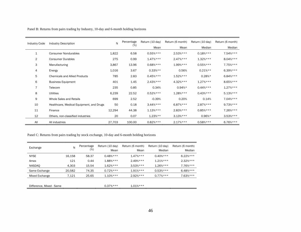
46

Panel B: Returns from pairs trading by Industry, 10-day and 6-month holding horizons

Industry Code Industry Description N Percentage

(%) Return (10 day) Return (6 month) Return (10 day) Return (6 month)

Mean Mean Median Median

1 Consumer Nondurables 1,822 6.58 0.55%*** 2.53%*** 0.18%*** 7.54%***

2 Consumer Durables 275 0.99 1.47%*** 2.47%*** 1.32%*** 8.04%***

3 Manufacturing 3,867 13.96 0.68%*** 1.99%*** 0.55%*** 7.75%***

4 Energy 1,016 3.67 0.33%** 0.56% 0.21%** 6.39%***

5 Chemicals and Allied Products 785 2.83 0.45%*** 1.52%*** 0.28%* 6.84%***

6 Business Equipment 401 1.45 2.43%*** 4.32%*** 1.27%*** 8.65%***

7 Telecom 235 0.85 0.34% 0.94%* 0.44%*** 1.27%***

8 Utilities 6,239 22.52 0.52%*** 1.28%*** 0.43%*** 5.13%***

9 Whole Sales and Retails 699 2.52 -0.39% 0.20% 0.14% 7.04%***

10 Healthcare, Medical Equipment, and Drugs 50 0.18 3.44%*** 6.87%*** 2.87%*** 9.73%***

11 Finance 12,294 44.38 1.13%*** 2.83%*** 0.85%*** 7.26%***

12 Others, non-classified industries 20 0.07 1.23%** 3.13%*** 0.96%* 3.53%***

All All industries 27,703 100.00 0.82%*** 2.17%*** 0.58%*** 6.76%***

Panel C: Returns from pairs trading by stock exchange, 10-day and 6-month holding horizons

Exchange N Percentage

(%) Return (10 day) Return (6 month) Return (10 day) Return (6 month)

Mean Mean Median Median

NYSE 16,158 58.37 0.48%*** 1.47%*** 0.40%*** 6.22%***

Amex 121 0.44 1.88%*** 2.49%*** 1.21%*** 2.32%***

NASDAQ 4,303 15.54 1.62%*** 3.53%*** 1.26%*** 7.76%***

Same Exchange 20,582 74.35 0.72%*** 1.91%*** 0.53%*** 6.48%***

Mixed Exchange 7,121 25.65 1.10%*** 2.92%*** 0.77%*** 7.63%***

Difference, Mixed - Same 0.37%*** 1.01%***

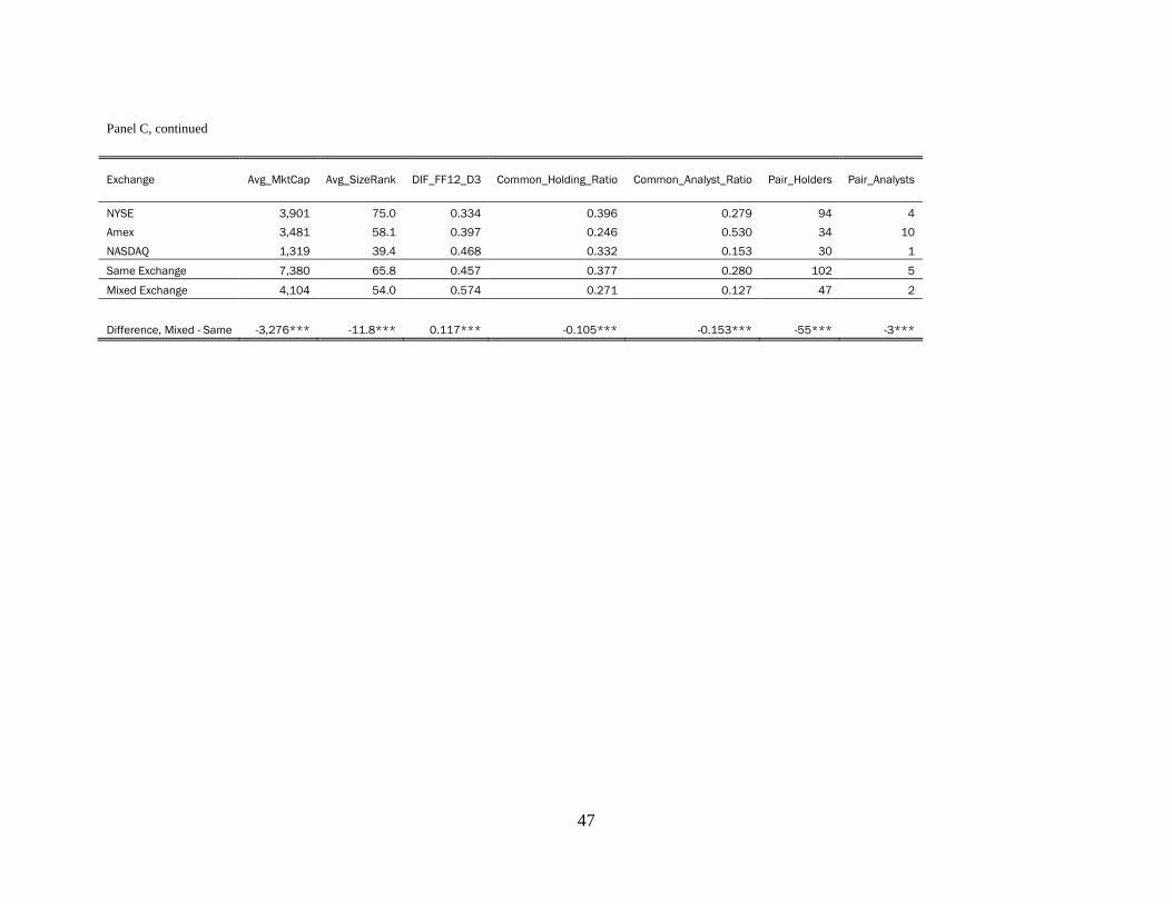
47

Panel C, continued

Exchange Avg_MktCap Avg_SizeRank DIF_FF12_D3 Common_Holding_Ratio Common_Analyst_Ratio Pair_Holders Pair_Analysts

NYSE 3,901 75.0 0.334 0.396 0.279 94 4

Amex 3,481 58.1 0.397 0.246 0.530 34 10

NASDAQ 1,319 39.4 0.468 0.332 0.153 30 1

Same Exchange 7,380 65.8 0.457 0.377 0.280 102 5

Mixed Exchange 4,104 54.0 0.574 0.271 0.127 47 2

Difference, Mixed - Same -3,276*** -11.8*** 0.117*** -0.105*** -0.153*** -55*** -3***

48

Table 2. Distribution of Select Corporate Events around Divergence Dates First four columns in Panel A report the distribution of select corporate events (quarterly earnings announcements, seasoned equity

offerings, mergers and acquisitions, debt issuance) within [t-1, t] two-day event window leading up to the date of pair divergence. Zero

stands for none of the constituent stocks of the pair experiences any corresponding corporate events, and one stands for at least one of the

constituent stocks of the pair experience the corresponding corporate events. The last column in Panel A, “All Events”, counts multiple

events happening within [t-1, t] two-day event window leading up to the date of pair divergence as one. Panel B is similar to Panel A, but

Panel B only consider the pairs where there is at least one piece of news coverage identified from Dow Jones News Wire (DJNW) news

database on the date of divergence.

Earnings

Announcement SEO

Mergers &

Acquisitions

Debt

Issuance All Events

Panel A: Number and percentage of select events within two-day window around date of pair divergence

0 26035 27673 27663 27554 25843

1 1668 30 40 149 1860

All 27703 27703 27703 27703 27703

0 93.98% 99.89% 99.86% 99.46% 93.29%

1 6.02% 0.11% 0.14% 0.54% 6.71%

All 100.00% 100.00% 100.00% 100.00% 100.00%

Panel B: Number and percentage of select events within two-day window around date of pair divergence, conditional on news

coverage

0 5743 6237 6223 6185 5661

1 503 9 23 61 585

All 6246 6246 6246 6246 6246

0 91.95% 99.86% 99.63% 99.02% 90.63%

1 8.05% 0.14% 0.37% 0.98% 9.37%

All 100.00% 100.00% 100.00% 100.00% 100.00%

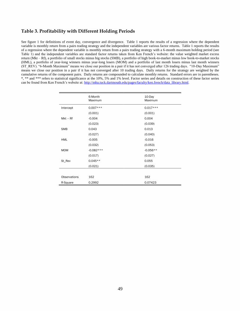
49

Table 3. Profitability with Different Holding Periods See figure 1 for definitions of event day, convergence and divergence. Table 1 reports the results of a regression where the dependent

variable is monthly return from a pairs trading strategy and the independent variables are various factor returns. Table 1 reports the results

of a regression where the dependent variable is monthly return from a pairs trading strategy with a 6-month maximum holding period (see

Table 1) and the independent variables are standard factor returns taken from Ken French’s website: the value weighted market excess

return (Mkt – Rf), a portfolio of small stocks minus big stocks (SMB), a portfolio of high book-to-market minus low book-to-market stocks

(HML), a portfolio of year-long winners minus year-long losers (MOM) and a portfolio of last month losers minus last month winners

(ST_REV). “6-Month Maximum” means we close our position in a pair if it has not converged after 126 trading days. “10-Day Maximum”

means we close our position in a pair if it has not converged after 10 trading days. Daily returns for the strategy are weighted by the

cumulative returns of the component pairs. Daily returns are compounded to calculate monthly returns. Standard errors are in parentheses.

*, ** and *** refers to statistical significance at the 10%, 5% and 1% level. Factor series and details on construction of these factor series

can be found from Ken French’s website at: http://mba.tuck.dartmouth.edu/pages/faculty/ken.french/data_library.html.

6-Month

Maximum

10-Day

Maximum

Intercept 0.007*** 0.017***

(0.001) (0.001)

Mkt – Rf -0.004 0.004

(0.023) (0.039)

SMB 0.043 0.013

(0.027) (0.040)

HML -0.005 -0.016

(0.032) (0.053)

MOM -0.082*** -0.056**

(0.017) (0.027)

St_Rev 0.045** 0.055

(0.021) (0.035)

Observations 162 162

R-Square 0.2992 0.07423

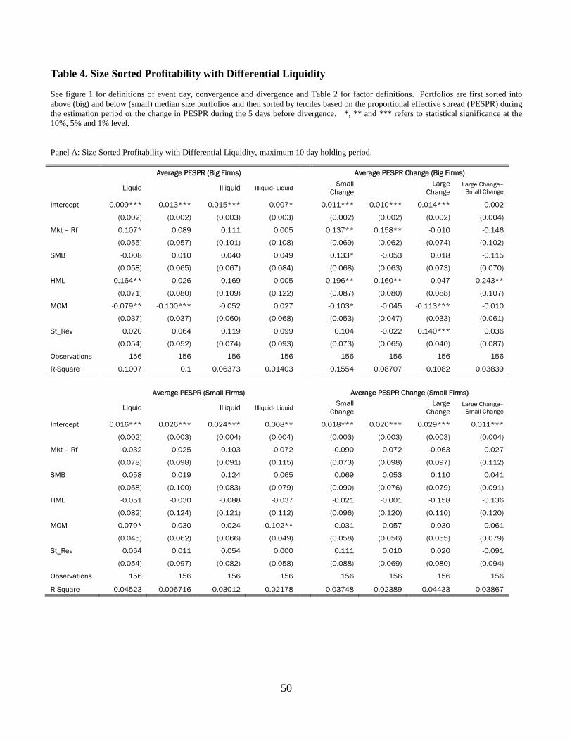
50

Table 4. Size Sorted Profitability with Differential Liquidity

See figure 1 for definitions of event day, convergence and divergence and Table 2 for factor definitions. Portfolios are first sorted into

above (big) and below (small) median size portfolios and then sorted by terciles based on the proportional effective spread (PESPR) during

the estimation period or the change in PESPR during the 5 days before divergence. *, ** and *** refers to statistical significance at the

10%, 5% and 1% level.

Panel A: Size Sorted Profitability with Differential Liquidity, maximum 10 day holding period.

Average PESPR (Big Firms) Average PESPR Change (Big Firms)

Liquid Illiquid Illiquid- Liquid Small

Change

Large

Change Large Change–

Small Change

Intercept 0.009*** 0.013*** 0.015*** 0.007* 0.011*** 0.010*** 0.014*** 0.002

(0.002) (0.002) (0.003) (0.003) (0.002) (0.002) (0.002) (0.004)

Mkt – Rf 0.107* 0.089 0.111 0.005 0.137** 0.158** -0.010 -0.146

(0.055) (0.057) (0.101) (0.108) (0.069) (0.062) (0.074) (0.102)

SMB -0.008 0.010 0.040 0.049 0.133* -0.053 0.018 -0.115

(0.058) (0.065) (0.067) (0.084) (0.068) (0.063) (0.073) (0.070)

HML 0.164** 0.026 0.169 0.005 0.196** 0.160** -0.047 -0.243**

(0.071) (0.080) (0.109) (0.122) (0.087) (0.080) (0.088) (0.107)

MOM -0.079** -0.100*** -0.052 0.027 -0.103* -0.045 -0.113*** -0.010

(0.037) (0.037) (0.060) (0.068) (0.053) (0.047) (0.033) (0.061)

St_Rev 0.020 0.064 0.119 0.099 0.104 -0.022 0.140*** 0.036

(0.054) (0.052) (0.074) (0.093) (0.073) (0.065) (0.040) (0.087)

Observations 156 156 156 156 156 156 156 156

R-Square 0.1007 0.1 0.06373 0.01403 0.1554 0.08707 0.1082 0.03839

Average PESPR (Small Firms) Average PESPR Change (Small Firms)

Liquid Illiquid Illiquid- Liquid Small

Change

Large

Change Large Change–

Small Change

Intercept 0.016*** 0.026*** 0.024*** 0.008** 0.018*** 0.020*** 0.029*** 0.011***

(0.002) (0.003) (0.004) (0.004) (0.003) (0.003) (0.003) (0.004)

Mkt – Rf -0.032 0.025 -0.103 -0.072 -0.090 0.072 -0.063 0.027

(0.078) (0.098) (0.091) (0.115) (0.073) (0.098) (0.097) (0.112)

SMB 0.058 0.019 0.124 0.065 0.069 0.053 0.110 0.041

(0.058) (0.100) (0.083) (0.079) (0.090) (0.076) (0.079) (0.091)

HML -0.051 -0.030 -0.088 -0.037 -0.021 -0.001 -0.158 -0.136

(0.082) (0.124) (0.121) (0.112) (0.096) (0.120) (0.110) (0.120)

MOM 0.079* -0.030 -0.024 -0.102** -0.031 0.057 0.030 0.061

(0.045) (0.062) (0.066) (0.049) (0.058) (0.056) (0.055) (0.079)

St_Rev 0.054 0.011 0.054 0.000 0.111 0.010 0.020 -0.091

(0.054) (0.097) (0.082) (0.058) (0.088) (0.069) (0.080) (0.094)

Observations 156 156 156 156 156 156 156 156

R-Square 0.04523 0.006716 0.03012 0.02178 0.03748 0.02389 0.04433 0.03867

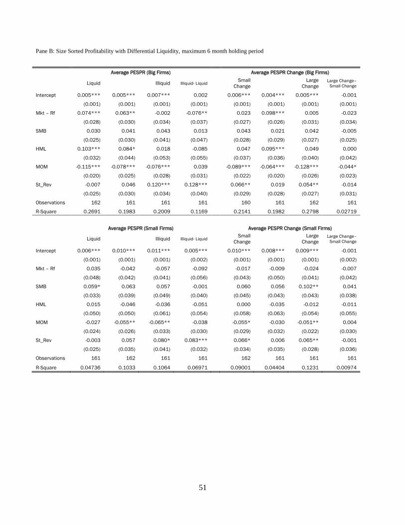
51

Pane B: Size Sorted Profitability with Differential Liquidity, maximum 6 month holding period

Average PESPR (Big Firms) Average PESPR Change (Big Firms)

Liquid Illiquid Illiquid- Liquid Small

Change

Large

Change Large Change–

Small Change

Intercept 0.005*** 0.005*** 0.007*** 0.002 0.006*** 0.004*** 0.005*** -0.001

(0.001) (0.001) (0.001) (0.001) (0.001) (0.001) (0.001) (0.001)

Mkt – Rf 0.074*** 0.063** -0.002 -0.076** 0.023 0.098*** 0.005 -0.023

(0.028) (0.030) (0.034) (0.037) (0.027) (0.026) (0.031) (0.034)

SMB 0.030 0.041 0.043 0.013 0.043 0.021 0.042 -0.005

(0.025) (0.030) (0.041) (0.047) (0.028) (0.029) (0.027) (0.025)

HML 0.103*** 0.084* 0.018 -0.085 0.047 0.095*** 0.049 0.000

(0.032) (0.044) (0.053) (0.055) (0.037) (0.036) (0.040) (0.042)

MOM -0.115*** -0.078*** -0.076*** 0.039 -0.089*** -0.064*** -0.128*** -0.044*

(0.020) (0.025) (0.028) (0.031) (0.022) (0.020) (0.026) (0.023)

St_Rev -0.007 0.046 0.120*** 0.128*** 0.066** 0.019 0.054** -0.014

(0.025) (0.030) (0.034) (0.040) (0.029) (0.028) (0.027) (0.031)

Observations 162 161 161 161 160 161 162 161

R-Square 0.2691 0.1983 0.2009 0.1169 0.2141 0.1982 0.2798 0.02719

Average PESPR (Small Firms) Average PESPR Change (Small Firms)

Liquid Illiquid Illiquid- Liquid Small

Change

Large

Change Large Change–

Small Change

Intercept 0.006*** 0.010*** 0.011*** 0.005*** 0.010*** 0.008*** 0.009*** -0.001

(0.001) (0.001) (0.001) (0.002) (0.001) (0.001) (0.001) (0.002)

Mkt – Rf 0.035 -0.042 -0.057 -0.092 -0.017 -0.009 -0.024 -0.007

(0.048) (0.042) (0.041) (0.056) (0.043) (0.050) (0.041) (0.042)

SMB 0.059* 0.063 0.057 -0.001 0.060 0.056 0.102** 0.041

(0.033) (0.039) (0.049) (0.040) (0.045) (0.043) (0.043) (0.038)

HML 0.015 -0.046 -0.036 -0.051 0.000 -0.035 -0.012 -0.011

(0.050) (0.050) (0.061) (0.054) (0.058) (0.063) (0.054) (0.055)

MOM -0.027 -0.055** -0.065** -0.038 -0.055* -0.030 -0.051** 0.004

(0.024) (0.026) (0.033) (0.030) (0.029) (0.032) (0.022) (0.030)

St_Rev -0.003 0.057 0.080* 0.083*** 0.066* 0.006 0.065** -0.001

(0.025) (0.035) (0.041) (0.032) (0.034) (0.035) (0.028) (0.036)

Observations 161 162 161 161 162 161 161 161

R-Square 0.04736 0.1033 0.1064 0.06971 0.09001 0.04404 0.1231 0.00974

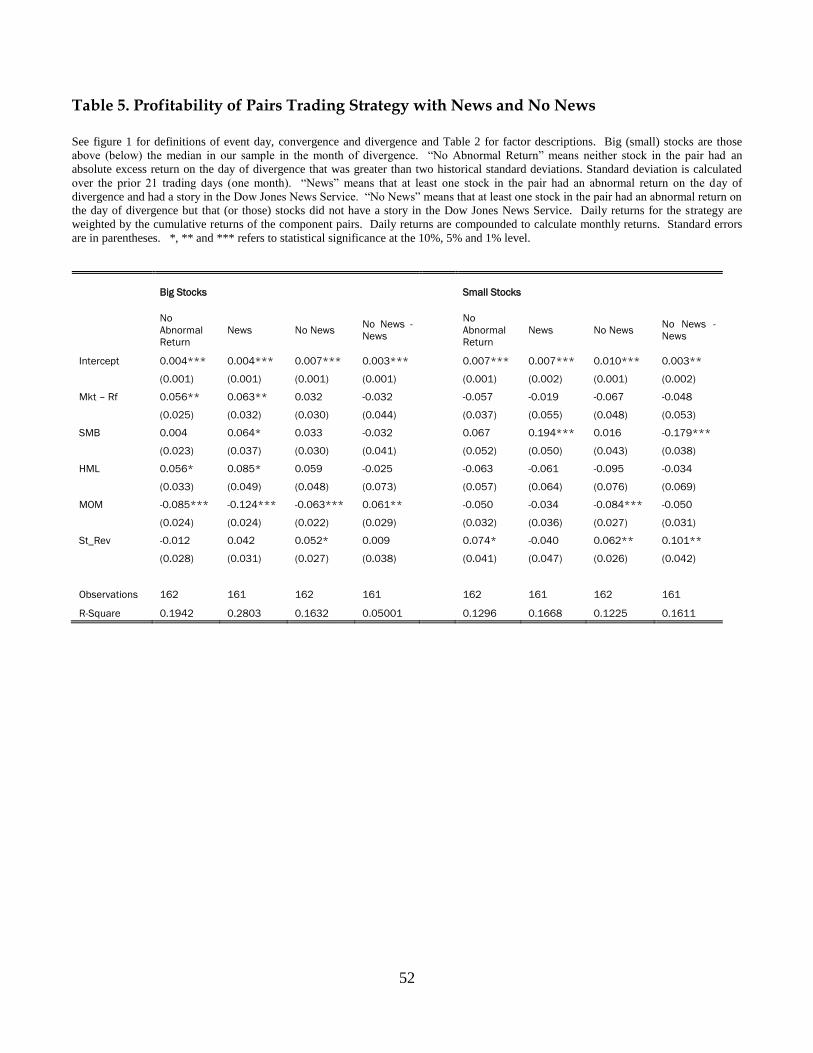
52

Table 5. Profitability of Pairs Trading Strategy with News and No News See figure 1 for definitions of event day, convergence and divergence and Table 2 for factor descriptions. Big (small) stocks are those

above (below) the median in our sample in the month of divergence. “No Abnormal Return” means neither stock in the pair had an

absolute excess return on the day of divergence that was greater than two historical standard deviations. Standard deviation is calculated

over the prior 21 trading days (one month). “News” means that at least one stock in the pair had an abnormal return on the day of

divergence and had a story in the Dow Jones News Service. “No News” means that at least one stock in the pair had an abnormal return on

the day of divergence but that (or those) stocks did not have a story in the Dow Jones News Service. Daily returns for the strategy are

weighted by the cumulative returns of the component pairs. Daily returns are compounded to calculate monthly returns. Standard errors

are in parentheses. *, ** and *** refers to statistical significance at the 10%, 5% and 1% level.

Big Stocks Small Stocks

No

Abnormal

Return

News No News No News -

News

No

Abnormal

Return

News No News No News -

News

Intercept 0.004*** 0.004*** 0.007*** 0.003*** 0.007*** 0.007*** 0.010*** 0.003**

(0.001) (0.001) (0.001) (0.001) (0.001) (0.002) (0.001) (0.002)

Mkt – Rf 0.056** 0.063** 0.032 -0.032 -0.057 -0.019 -0.067 -0.048

(0.025) (0.032) (0.030) (0.044) (0.037) (0.055) (0.048) (0.053)

SMB 0.004 0.064* 0.033 -0.032 0.067 0.194*** 0.016 -0.179***

(0.023) (0.037) (0.030) (0.041) (0.052) (0.050) (0.043) (0.038)

HML 0.056* 0.085* 0.059 -0.025 -0.063 -0.061 -0.095 -0.034

(0.033) (0.049) (0.048) (0.073) (0.057) (0.064) (0.076) (0.069)

MOM -0.085*** -0.124*** -0.063*** 0.061** -0.050 -0.034 -0.084*** -0.050

(0.024) (0.024) (0.022) (0.029) (0.032) (0.036) (0.027) (0.031)

St_Rev -0.012 0.042 0.052* 0.009 0.074* -0.040 0.062** 0.101**

(0.028) (0.031) (0.027) (0.038) (0.041) (0.047) (0.026) (0.042)

Observations 162 161 162 161 162 161 162 161

R-Square 0.1942 0.2803 0.1632 0.05001 0.1296 0.1668 0.1225 0.1611

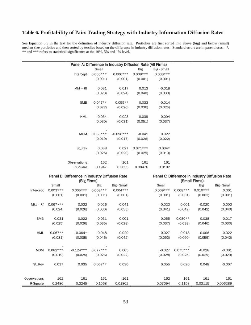
53

Table 6. Profitability of Pairs Trading Strategy with Industry Information Diffusion Rates

See Equation 5.5 in the text for the definition of industry diffusion rate. Portfolios are first sorted into above (big) and below (small)

median size portfolios and then sorted by terciles based on the difference in industry diffusion rates. Standard errors are in parentheses. *,

** and *** refers to statistical significance at the 10%, 5% and 1% level.

Panel A: Difference in Industry Diffusion Rate (All Firms) Small Big Big - Small

Intercept 0.005*** 0.006*** 0.009*** 0.003***

(0.001) (0.001) (0.001) (0.001)

Mkt – Rf 0.031 0.017 0.013 -0.018

(0.023) (0.024) (0.040) (0.033)

SMB 0.047** 0.055** 0.033 -0.014

(0.022) (0.026) (0.036) (0.025)

HML 0.034 0.023 0.039 0.004

(0.030) (0.031) (0.051) (0.037)

MOM

-

0.063*** -0.098*** -0.041 0.022

(0.019) (0.017) (0.026) (0.022)

St_Rev 0.038 0.027 0.071*** 0.034*

(0.025) (0.020) (0.025) (0.019)

Observations 162 161 161 161

R-Square 0.1947 0.3055 0.08476 0.0182

Panel B: Difference in Industry Diffusion Rate

(Big Firms)

Panel C: Difference in Industry Diffusion Rate

(Small Firms) Small Big Big - Small Small Big Big - Small

Intercept 0.003*** 0.005*** 0.008*** 0.004*** 0.009*** 0.008*** 0.010*** 0.001

(0.001) (0.001) (0.001) (0.001) (0.001) (0.001) (0.002) (0.001)

Mkt – Rf 0.067*** 0.022 0.026 -0.041 -0.022 0.001 -0.020 0.002

(0.024) (0.026) (0.036) (0.033) (0.041) (0.042) (0.042) (0.040)

SMB 0.031 0.022 0.031 0.001 0.055 0.080** 0.038 -0.017

(0.025) (0.026) (0.035) (0.028) (0.037) (0.038) (0.046) (0.030)

HML 0.067** 0.064* 0.048 -0.020 -0.027 -0.018 -0.006 0.022

(0.031) (0.035) (0.046) (0.042) (0.050) (0.060) (0.059) (0.042)

MOM

-

0.082*** -0.124***

-

0.077*** 0.005 -0.027

-

0.075*** -0.028 -0.001

(0.019) (0.025) (0.026) (0.022) (0.028) (0.025) (0.029) (0.029)

St_Rev 0.037 0.035 0.067** 0.030 0.055 0.026 0.048 -0.007

Observations 162 161 161 161 162 161 161 161

R-Square 0.2486 0.2245 0.1568 0.01802 0.07094 0.1158 0.03115 0.006289

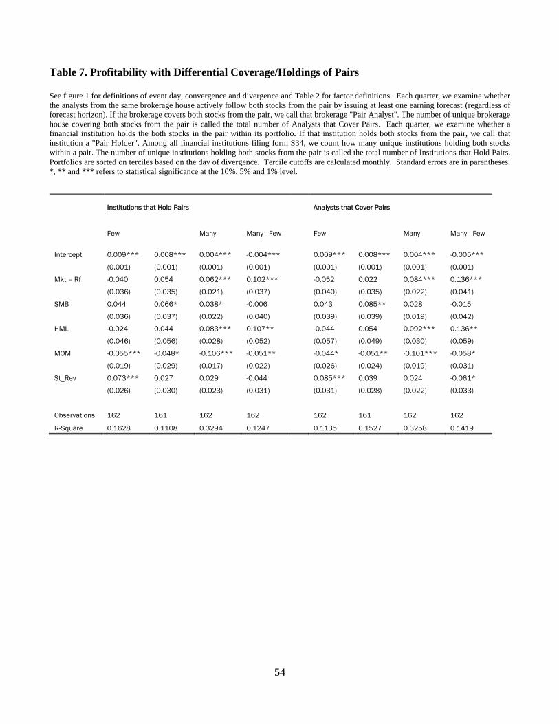
54

Table 7. Profitability with Differential Coverage/Holdings of Pairs

See figure 1 for definitions of event day, convergence and divergence and Table 2 for factor definitions. Each quarter, we examine whether

the analysts from the same brokerage house actively follow both stocks from the pair by issuing at least one earning forecast (regardless of

forecast horizon). If the brokerage covers both stocks from the pair, we call that brokerage "Pair Analyst". The number of unique brokerage

house covering both stocks from the pair is called the total number of Analysts that Cover Pairs. Each quarter, we examine whether a

financial institution holds the both stocks in the pair within its portfolio. If that institution holds both stocks from the pair, we call that

institution a "Pair Holder". Among all financial institutions filing form S34, we count how many unique institutions holding both stocks

within a pair. The number of unique institutions holding both stocks from the pair is called the total number of Institutions that Hold Pairs.

Portfolios are sorted on terciles based on the day of divergence. Tercile cutoffs are calculated monthly. Standard errors are in parentheses.

*, ** and *** refers to statistical significance at the 10%, 5% and 1% level.

Institutions that Hold Pairs Analysts that Cover Pairs

Few Many Many - Few Few Many Many - Few

Intercept 0.009*** 0.008*** 0.004*** -0.004*** 0.009*** 0.008*** 0.004*** -0.005***

(0.001) (0.001) (0.001) (0.001) (0.001) (0.001) (0.001) (0.001)

Mkt – Rf -0.040 0.054 0.062*** 0.102*** -0.052 0.022 0.084*** 0.136***

(0.036) (0.035) (0.021) (0.037) (0.040) (0.035) (0.022) (0.041)

SMB 0.044 0.066* 0.038* -0.006 0.043 0.085** 0.028 -0.015

(0.036) (0.037) (0.022) (0.040) (0.039) (0.039) (0.019) (0.042)

HML -0.024 0.044 0.083*** 0.107** -0.044 0.054 0.092*** 0.136**

(0.046) (0.056) (0.028) (0.052) (0.057) (0.049) (0.030) (0.059)

MOM -0.055*** -0.048* -0.106*** -0.051** -0.044* -0.051** -0.101*** -0.058*

(0.019) (0.029) (0.017) (0.022) (0.026) (0.024) (0.019) (0.031)

St_Rev 0.073*** 0.027 0.029 -0.044 0.085*** 0.039 0.024 -0.061*

(0.026) (0.030) (0.023) (0.031) (0.031) (0.028) (0.022) (0.033)

Observations 162 161 162 162 162 161 162 162

R-Square 0.1628 0.1108 0.3294 0.1247 0.1135 0.1527 0.3258 0.1419

55

Table 8. Size Sorted Profitability with Differential Coverage/Holdings of Pairs

See Table 7 for definitions. Portfolios are first sorted into above (big) and below (small) median size portfolios and then sorted by terciles

as in Table 7. Standard errors are in parentheses. *, ** and *** refers to statistical significance at the 10%, 5% and 1% level.

Institutions that Hold Pairs (Big Firms) Institutions that Hold Pairs (Small Firms)

Few Many Many - Few Few Many Many - Few

Intercept 0.007*** 0.004*** 0.005*** -0.002* 0.010*** 0.009*** 0.008*** -0.001

(0.001) (0.001) (0.001) (0.001) (0.001) (0.002) (0.001) (0.002)

Mkt – Rf -0.001 0.072** 0.066** 0.066 -0.042 -0.021 0.021 0.063

(0.041) (0.028) (0.026) (0.043) (0.042) (0.052) (0.037) (0.047)

SMB 0.063 0.018 0.032 -0.030 -0.001 0.104** 0.098** 0.098**

(0.044) (0.025) (0.027) (0.048) (0.039) (0.046) (0.047) (0.042)

HML 0.053 0.083** 0.076** 0.023 -0.058 0.006 0.014 0.072

(0.062) (0.040) (0.034) (0.069) (0.056) (0.073) (0.047) (0.057)

MOM -0.051 -0.073*** -0.145*** -0.094** -0.026 -0.064** -0.041 -0.015

(0.031) (0.022) (0.024) (0.037) (0.029) (0.027) (0.027) (0.033)

St_Rev 0.085** 0.064*** 0.004 -0.080* 0.067** 0.057* 0.006 -0.062*

(0.036) (0.022) (0.033) (0.043) (0.032) (0.034) (0.035) (0.033)

Observations 161 162 161 161 162 161 161 161

R-Square 0.118 0.2071 0.3265 0.107 0.05143 0.0987 0.1042 0.057

Analysts that Cover Pairs (Big Firms) Analysts that Cover Pairs (Small Firms)

Few Many Many - Few Few Many Many - Few

Intercept 0.007*** 0.004*** 0.004*** -0.003** 0.008*** 0.011*** 0.009*** 0.000

(0.001) (0.001) (0.001) (0.001) (0.001) (0.002) (0.002) (0.001)

Mkt – Rf 0.009 0.084*** 0.073*** 0.064* -0.036 0.009 -0.011 0.025

(0.036) (0.029) (0.024) (0.038) (0.039) (0.079) (0.052) (0.040)

SMB 0.033 0.052 0.036 0.004 0.048 -0.046 0.081* 0.033

(0.037) (0.032) (0.025) (0.042) (0.041) (0.091) (0.042) (0.035)

HML 0.018 0.114*** 0.107*** 0.088 -0.034 0.100 -0.057 -0.023

(0.057) (0.042) (0.032) (0.056) (0.052) (0.099) (0.064) (0.051)

MOM -0.053* -0.114*** -0.107*** -0.054* -0.057** -0.042 -0.027 0.031

(0.030) (0.021) (0.019) (0.030) (0.022) (0.051) (0.036) (0.032)

St_Rev 0.083*** 0.058** -0.001 -0.084** 0.058** 0.039 0.029 -0.029

(0.031) (0.029) (0.028) (0.033) (0.028) (0.051) (0.039) (0.033)

Observations 161 162 161 161 162 152 161 161

R-Square 0.1184 0.3114 0.2612 0.08887 0.1022 0.04431 0.07114 0.03366

56

Table 9. Time-series Cross-Sectional Regressions of Pairs Returns on Pairs Characteristics

This table reports the time-series cross-sectional regression of individual pair’s profits (dependent variable) on the pair’s characteristics

(independent variables). In Panel A and Panel C, the profits are computed from a strategy of maximum holding horizon of 10 days. In

Panel B and Panel D, the profits are computed from a strategy of maximum holding horizon of 6 months. Panel A (Panel C) and Panel B

(Panel D) differ in terms of independent variables. Compared with Panel A (Panel C), Panel B (Panel D) include industry information

diffusion measure (DIF_FF12_D3) as well as its interaction with Size, Liquidity, Common Analyst Coverage and Common Institutional

Holding variables. Several pairs characteristics control variables, including Avg_Ret_pst1mth, Avg_Ret_pst12mth, Avg_Ret_pst36mth,

Avg_BM, Log_Avg_MktCap, Avg_mRetVola, though included in the regressions of Panel C and Panel D, are not reported to preserve

brevity. Avg_PESPR is the pair’s average proportional effective spreads, measured during the pair formation period. Avg_PESPR_Change

is the change of the average of the pair’s proportional effective spreads, measured in the previous five days leading to the event day minus

the pair’s average proportional effective spreads, measured during the pair formation period. Avg_Turn is the pair’s average daily turnover

ratio, measured during the pair formation period. Avg_dTurn_Change is the change of the average of the pair’s daily turnover ratio,

measured in the previous five days leading to the event day; minus the pair’s average daily turnover ratio, measured during the pair

formation period. News is defined in Table 5 and Coverage is “No News” from Table 2. Avg_Ret_pst1mth is the pair’s average

cumulative returns over the one month prior to the event month (event month is the month when the event date occurs). Avg_Ret_pst12mth

is the pair’s average cumulative return over the eleven months prior to the second month to the event month. Avg_Ret_pst36mth is the

pair’s average cumulative return over the 24 months prior to the twelve month to the event month. Avg_BM is the pair’s average book to

market equity ratios measured using the most recently available book equity value, and the market equity values during the month ending at

the beginning of the previous month. Log_Avg_MktCap is the logarithm of market capitalization of firms in billion dollars using last

available market capitalization t during the estimation period. Avg_mRetVola is the average of the pair’s monthly return volatilities during

estimation period. Common_Holding_Ratio is the number of institutions holding both stocks in the pair during the quarter prior to the

event quarter (the quarter the event date occurs), divided by the maximum number of institutions holding stock one or stock two of the pair

during the same quarter. If the number of institutions holding two stocks of the pair is less than fifty, the Common_Holding indicator

variable takes the value of one; and zero otherwise. Common_Coverage_Ratio is the number of brokerage houses (as identified by the

brokerage code in I/B/E/S), divided by the maximum number of brokerage houses covering stock one or stock two of the pair during the

same quarter. If the number of brokerage houses covering two stocks of the pair is less than or equal to two, the Common_Coverage

indicator variable takes the value of one; and zero otherwise. Size_Rank takes the value of one if the average size percentile of the pair is

below 50-th, and zero otherwise. In regressions 3 of both Panel A and Panel B, the common institutional holding and common analyst

coverage variables are continuous variables. In regressions 4 and 5 of both Panel A and Panel B, the common institutional holding and

common analyst coverage variables are binary dummy variables, which take the value of one if the value of the variable is below sample

median, and zero otherwise. All regressions compute the clustered standard errors, where the cluster is defined by year, month and

industry. Standard errors are in parentheses. *, ** and *** refers to statistical significance at the 10%, 5% and 1% level.

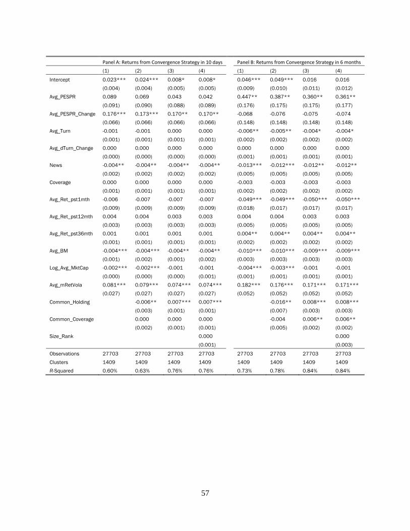
57

Panel A: Returns from Convergence Strategy in 10 days

Panel B: Returns from Convergence Strategy in 6 months

(1) (2) (3) (4)

(1) (2) (3) (4)

Intercept 0.023*** 0.024*** 0.008* 0.008*

0.046*** 0.049*** 0.016 0.016

(0.004) (0.004) (0.005) (0.005)

(0.009) (0.010) (0.011) (0.012)

Avg_PESPR 0.089 0.069 0.043 0.042

0.447** 0.387** 0.360** 0.361**

(0.091) (0.090) (0.088) (0.089)

(0.176) (0.175) (0.175) (0.177)

Avg_PESPR_Change 0.176*** 0.173*** 0.170** 0.170**

-0.068 -0.076 -0.075 -0.074

(0.066) (0.066) (0.066) (0.066)

(0.148) (0.148) (0.148) (0.148)

Avg_Turn -0.001 -0.001 0.000 0.000

-0.006** -0.005** -0.004* -0.004*

(0.001) (0.001) (0.001) (0.001)

(0.002) (0.002) (0.002) (0.002)

Avg_dTurn_Change 0.000 0.000 0.000 0.000

0.000 0.000 0.000 0.000

(0.000) (0.000) (0.000) (0.000)

(0.001) (0.001) (0.001) (0.001)

News -0.004** -0.004** -0.004** -0.004**

-0.013*** -0.012*** -0.012** -0.012**

(0.002) (0.002) (0.002) (0.002)

(0.005) (0.005) (0.005) (0.005)

Coverage 0.000 0.000 0.000 0.000

-0.003 -0.003 -0.003 -0.003

(0.001) (0.001) (0.001) (0.001)

(0.002) (0.002) (0.002) (0.002)

Avg_Ret_pst1mth -0.006 -0.007 -0.007 -0.007

-0.049*** -0.049*** -0.050*** -0.050***

(0.009) (0.009) (0.009) (0.009)

(0.018) (0.017) (0.017) (0.017)

Avg_Ret_pst12mth 0.004 0.004 0.003 0.003

0.004 0.004 0.003 0.003

(0.003) (0.003) (0.003) (0.003)

(0.005) (0.005) (0.005) (0.005)

Avg_Ret_pst36mth 0.001 0.001 0.001 0.001

0.004** 0.004** 0.004** 0.004**

(0.001) (0.001) (0.001) (0.001)

(0.002) (0.002) (0.002) (0.002)

Avg_BM -0.004*** -0.004*** -0.004** -0.004**

-0.010*** -0.010*** -0.009*** -0.009***

(0.001) (0.002) (0.001) (0.002)

(0.003) (0.003) (0.003) (0.003)

Log_Avg_MktCap -0.002*** -0.002*** -0.001 -0.001

-0.004*** -0.003*** -0.001 -0.001

(0.000) (0.000) (0.000) (0.001)

(0.001) (0.001) (0.001) (0.001)

Avg_mRetVola 0.081*** 0.079*** 0.074*** 0.074***

0.182*** 0.176*** 0.171*** 0.171***

(0.027) (0.027) (0.027) (0.027)

(0.052) (0.052) (0.052) (0.052)

Common_Holding -0.006** 0.007*** 0.007***

-0.016** 0.008*** 0.008***

(0.003) (0.001) (0.001)

(0.007) (0.003) (0.003)

Common_Coverage 0.000 0.000 0.000

-0.004 0.006** 0.006**

(0.002) (0.001) (0.001)

(0.005) (0.002) (0.002)

Size_Rank 0.000

0.000

(0.001)

(0.003)

Observations 27703 27703 27703 27703

27703 27703 27703 27703

Clusters 1409 1409 1409 1409

1409 1409 1409 1409

R-Squared 0.60% 0.63% 0.76% 0.76%

0.73% 0.78% 0.84% 0.84%

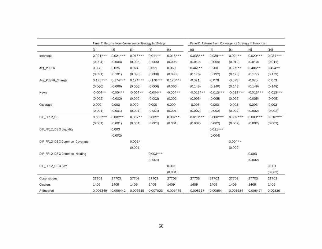
58

Panel C: Returns from Convergence Strategy in 10 days Panel D: Returns from Convergence Strategy in 6 months

(1) (2) (3) (4) (5) (6) (7) (8) (9) (10)

Intercept 0.021*** 0.021*** 0.016*** 0.011** 0.016*** 0.038*** 0.039*** 0.024** 0.029*** 0.034***

(0.004) (0.004) (0.005) (0.005) (0.005) (0.010) (0.009) (0.010) (0.010) (0.011)

Avg_PESPR 0.088 0.025 0.074 0.051 0.069 0.441** 0.200 0.399** 0.406** 0.424**

(0.091) (0.101) (0.090) (0.088) (0.090) (0.176) (0.192) (0.176) (0.177) (0.179)

Avg_PESPR_Change 0.175*** 0.174*** 0.174*** 0.170*** 0.173*** -0.071 -0.076 -0.073 -0.075 -0.073

(0.066) (0.066) (0.066) (0.066) (0.066) (0.148) (0.149) (0.148) (0.148) (0.148)

News -0.004** -0.004** -0.004** -0.004** -0.004** -0.013*** -0.013*** -0.013*** -0.013*** -0.013***

(0.002) (0.002) (0.002) (0.002) (0.002) (0.005) (0.005) (0.005) (0.005) (0.005)

Coverage 0.000 0.000 0.000 0.000 0.000 -0.003 -0.003 -0.003 -0.003 -0.003

(0.001) (0.001) (0.001) (0.001) (0.001) (0.002) (0.002) (0.002) (0.002) (0.002)

DIF_FF12_D3 0.003*** 0.002** 0.002** 0.002* 0.002** 0.010*** 0.008*** 0.009*** 0.009*** 0.010***

(0.001) (0.001) (0.001) (0.001) (0.001) (0.002) (0.002) (0.002) (0.002) (0.002)

DIF_FF12_D3 X Liquidity 0.003 0.011***

(0.002) (0.004)

DIF_FF12_D3 X Common_Coverage 0.001* 0.004**

(0.001) (0.002)

DIF_FF12_D3 X Common_Holding 0.003*** 0.003

(0.001) (0.002)

DIF_FF12_D3 X Size 0.001 0.001

(0.001) (0.002)

Observations 27703 27703 27703 27703 27703 27703 27703 27703 27703 27703

Clusters 1409 1409 1409 1409 1409 1409 1409 1409 1409 1409

R-Squared 0.006349 0.006442 0.006515 0.007023 0.006475 0.008337 0.00864 0.008684 0.008474 0.00836

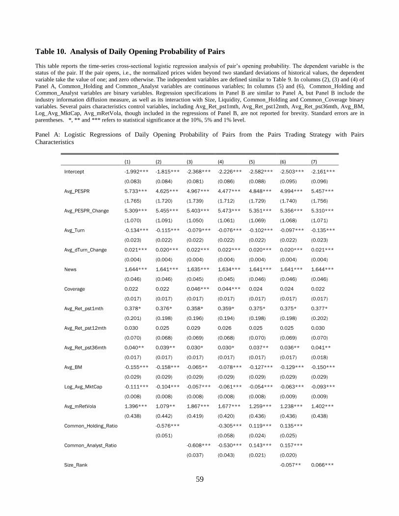
59

Table 10. Analysis of Daily Opening Probability of Pairs

This table reports the time-series cross-sectional logistic regression analysis of pair’s opening probability. The dependent variable is the

status of the pair. If the pair opens, i.e., the normalized prices widen beyond two standard deviations of historical values, the dependent

variable take the value of one; and zero otherwise. The independent variables are defined similar to Table 9. In columns (2), (3) and (4) of

Panel A, Common_Holding and Common_Analyst variables are continuous variables; In columns (5) and (6), Common_Holding and

Common_Analyst variables are binary variables. Regression specifications in Panel B are similar to Panel A, but Panel B include the

industry information diffusion measure, as well as its interaction with Size, Liquidity, Common_Holding and Common_Coverage binary

variables. Several pairs characteristics control variables, including Avg_Ret_pst1mth, Avg_Ret_pst12mth, Avg_Ret_pst36mth, Avg_BM,

Log_Avg_MktCap, Avg_mRetVola, though included in the regressions of Panel B, are not reported for brevity. Standard errors are in

parentheses. *, ** and *** refers to statistical significance at the 10%, 5% and 1% level.

Panel A: Logistic Regressions of Daily Opening Probability of Pairs from the Pairs Trading Strategy with Pairs

Characteristics

(1) (2) (3) (4) (5) (6) (7)

Intercept -1.992*** -1.815*** -2.368*** -2.226*** -2.582*** -2.503*** -2.161***

(0.083) (0.084) (0.081) (0.086) (0.088) (0.095) (0.096)

Avg_PESPR 5.733*** 4.625*** 4.967*** 4.477*** 4.848*** 4.994*** 5.457***

(1.765) (1.720) (1.739) (1.712) (1.729) (1.740) (1.756)

Avg_PESPR_Change 5.309*** 5.455*** 5.403*** 5.473*** 5.351*** 5.356*** 5.310***

(1.070) (1.091) (1.050) (1.061) (1.069) (1.068) (1.071)

Avg_Turn -0.134*** -0.115*** -0.079*** -0.076*** -0.102*** -0.097*** -0.135***

(0.023) (0.022) (0.022) (0.022) (0.022) (0.022) (0.023)

Avg_dTurn_Change 0.021*** 0.020*** 0.022*** 0.022*** 0.020*** 0.020*** 0.021***

(0.004) (0.004) (0.004) (0.004) (0.004) (0.004) (0.004)

News 1.644*** 1.641*** 1.635*** 1.634*** 1.641*** 1.641*** 1.644***

(0.046) (0.046) (0.045) (0.045) (0.046) (0.046) (0.046)

Coverage 0.022 0.022 0.046*** 0.044*** 0.024 0.024 0.022

(0.017) (0.017) (0.017) (0.017) (0.017) (0.017) (0.017)

Avg_Ret_pst1mth 0.378* 0.376* 0.358* 0.359* 0.375* 0.375* 0.377*

(0.201) (0.198) (0.196) (0.194) (0.198) (0.198) (0.202)

Avg_Ret_pst12mth 0.030 0.025 0.029 0.026 0.025 0.025 0.030

(0.070) (0.068) (0.069) (0.068) (0.070) (0.069) (0.070)

Avg_Ret_pst36mth 0.040** 0.039** 0.030* 0.030* 0.037** 0.036** 0.041**

(0.017) (0.017) (0.017) (0.017) (0.017) (0.017) (0.018)

Avg_BM -0.155*** -0.158*** -0.065** -0.078*** -0.127*** -0.129*** -0.150***

(0.029) (0.029) (0.029) (0.029) (0.029) (0.029) (0.029)

Log_Avg_MktCap -0.111*** -0.104*** -0.057*** -0.061*** -0.054*** -0.063*** -0.093***

(0.008) (0.008) (0.008) (0.008) (0.008) (0.009) (0.009)

Avg_mRetVola 1.396*** 1.079** 1.867*** 1.677*** 1.259*** 1.238*** 1.402***

(0.438) (0.442) (0.419) (0.420) (0.436) (0.436) (0.438)

Common_Holding_Ratio -0.576*** -0.305*** 0.119*** 0.135***

(0.051) (0.058) (0.024) (0.025)

Common_Analyst_Ratio -0.608*** -0.530*** 0.143*** 0.157***

(0.037) (0.043) (0.021) (0.020)

Size_Rank -0.057** 0.066***

60

(0.025) (0.023)

Observations 825,962 825,962 825,962 825,962 825962 825,962 825,962

Clusters 1587 1587 1587 1587 1587 1587 1587

Panel B: Logistic Regressions of Daily Opening Probability of Pairs from the Pairs Trading Strategy with Pairs

Characteristics, with additional industry information diffusion measure and its interactions with Size, Liquidity, Common

Institutional Ownership and Common Analyst Coverage

(1) (2) (3) (4) (5)

Intercept -2.114*** -2.118*** -2.118*** -2.554*** -2.293***

(0.084) (0.082) (0.083) (0.091) (0.096)

Avg_PESPR 5.816*** 3.529* 5.081** 5.072*** 5.425***

(1.740) (1.814) (2.067) (1.717) (1.732)

Avg_PESPR_Change 5.340*** 5.433*** 5.358*** 5.358*** 5.349***

(1.062) (1.065) (1.062) (1.062) (1.063)

Avg_Turn -0.128*** -0.127*** -0.128*** -0.095*** -0.123***

(0.023) (0.023) (0.023) (0.023) (0.023)

Avg_dTurn_Change 0.021*** 0.021*** 0.021*** 0.021*** 0.021***

(0.004) (0.004) (0.004) (0.004) (0.004)

News 1.642*** 1.642*** 1.642*** 1.640*** 1.642***

(0.046) (0.046) (0.046) (0.046) (0.046)

Coverage 0.023 0.023 0.023 0.023 0.022

(0.017) (0.017) (0.017) (0.017) (0.017)

DIF_F12_D3 0.131*** 0.102*** 0.132*** 0.088*** 0.118***

(0.016) (0.018) (0.017) (0.016) (0.017)

DIF_F12_D3 x Liquidity 0.137***

(0.029)

DIF_F12_D3 x Common_Holding 0.058

(0.071)

DIF_F12_D3 x Common_Analyst 0.131***

(0.014)

DIF_F12_D3 x Size 0.050***

(0.016)

Observations 825962 825962 825962 825962 825962

Clusters 1587 1587 1587 1587 1587

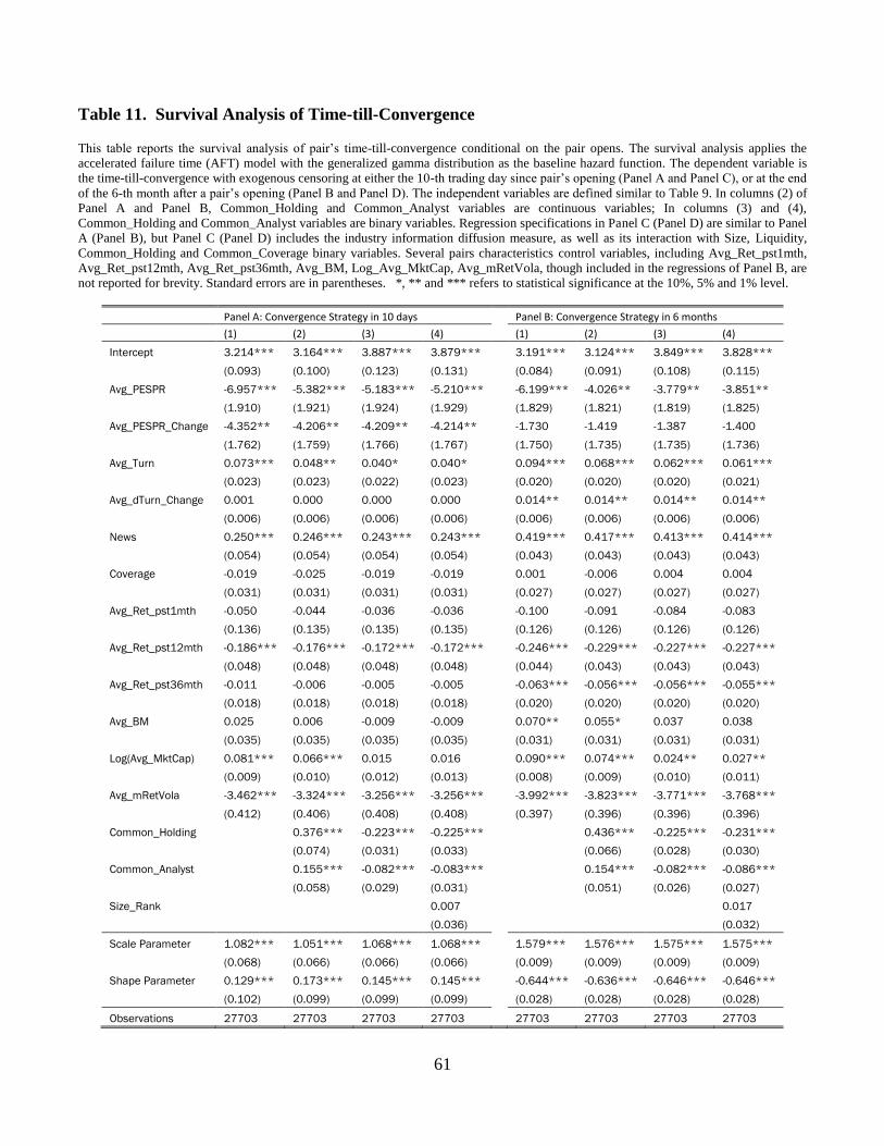
61

Table 11. Survival Analysis of Time-till-Convergence This table reports the survival analysis of pair’s time-till-convergence conditional on the pair opens. The survival analysis applies the

accelerated failure time (AFT) model with the generalized gamma distribution as the baseline hazard function. The dependent variable is

the time-till-convergence with exogenous censoring at either the 10-th trading day since pair’s opening (Panel A and Panel C), or at the end

of the 6-th month after a pair’s opening (Panel B and Panel D). The independent variables are defined similar to Table 9. In columns (2) of

Panel A and Panel B, Common_Holding and Common_Analyst variables are continuous variables; In columns (3) and (4),

Common_Holding and Common_Analyst variables are binary variables. Regression specifications in Panel C (Panel D) are similar to Panel

A (Panel B), but Panel C (Panel D) includes the industry information diffusion measure, as well as its interaction with Size, Liquidity,

Common_Holding and Common_Coverage binary variables. Several pairs characteristics control variables, including Avg_Ret_pst1mth,

Avg_Ret_pst12mth, Avg_Ret_pst36mth, Avg_BM, Log_Avg_MktCap, Avg_mRetVola, though included in the regressions of Panel B, are

not reported for brevity. Standard errors are in parentheses. *, ** and *** refers to statistical significance at the 10%, 5% and 1% level.

Panel A: Convergence Strategy in 10 days Panel B: Convergence Strategy in 6 months

(1) (2) (3) (4) (1) (2) (3) (4)

Intercept 3.214*** 3.164*** 3.887*** 3.879*** 3.191*** 3.124*** 3.849*** 3.828***

(0.093) (0.100) (0.123) (0.131) (0.084) (0.091) (0.108) (0.115)

Avg_PESPR -6.957*** -5.382*** -5.183*** -5.210*** -6.199*** -4.026** -3.779** -3.851**

(1.910) (1.921) (1.924) (1.929) (1.829) (1.821) (1.819) (1.825)

Avg_PESPR_Change -4.352** -4.206** -4.209** -4.214** -1.730 -1.419 -1.387 -1.400

(1.762) (1.759) (1.766) (1.767) (1.750) (1.735) (1.735) (1.736)

Avg_Turn 0.073*** 0.048** 0.040* 0.040* 0.094*** 0.068*** 0.062*** 0.061***

(0.023) (0.023) (0.022) (0.023) (0.020) (0.020) (0.020) (0.021)

Avg_dTurn_Change 0.001 0.000 0.000 0.000 0.014** 0.014** 0.014** 0.014**

(0.006) (0.006) (0.006) (0.006) (0.006) (0.006) (0.006) (0.006)

News 0.250*** 0.246*** 0.243*** 0.243*** 0.419*** 0.417*** 0.413*** 0.414***

(0.054) (0.054) (0.054) (0.054) (0.043) (0.043) (0.043) (0.043)

Coverage -0.019 -0.025 -0.019 -0.019 0.001 -0.006 0.004 0.004

(0.031) (0.031) (0.031) (0.031) (0.027) (0.027) (0.027) (0.027)

Avg_Ret_pst1mth -0.050 -0.044 -0.036 -0.036 -0.100 -0.091 -0.084 -0.083

(0.136) (0.135) (0.135) (0.135) (0.126) (0.126) (0.126) (0.126)

Avg_Ret_pst12mth -0.186*** -0.176*** -0.172*** -0.172*** -0.246*** -0.229*** -0.227*** -0.227***

(0.048) (0.048) (0.048) (0.048) (0.044) (0.043) (0.043) (0.043)

Avg_Ret_pst36mth -0.011 -0.006 -0.005 -0.005 -0.063*** -0.056*** -0.056*** -0.055***

(0.018) (0.018) (0.018) (0.018) (0.020) (0.020) (0.020) (0.020)

Avg_BM 0.025 0.006 -0.009 -0.009 0.070** 0.055* 0.037 0.038

(0.035) (0.035) (0.035) (0.035) (0.031) (0.031) (0.031) (0.031)

Log(Avg_MktCap) 0.081*** 0.066*** 0.015 0.016 0.090*** 0.074*** 0.024** 0.027**

(0.009) (0.010) (0.012) (0.013) (0.008) (0.009) (0.010) (0.011)

Avg_mRetVola -3.462*** -3.324*** -3.256*** -3.256*** -3.992*** -3.823*** -3.771*** -3.768***

(0.412) (0.406) (0.408) (0.408) (0.397) (0.396) (0.396) (0.396)

Common_Holding 0.376*** -0.223*** -0.225*** 0.436*** -0.225*** -0.231***

(0.074) (0.031) (0.033) (0.066) (0.028) (0.030)

Common_Analyst 0.155*** -0.082*** -0.083*** 0.154*** -0.082*** -0.086***

(0.058) (0.029) (0.031) (0.051) (0.026) (0.027)

Size_Rank 0.007 0.017

(0.036) (0.032)

Scale Parameter 1.082*** 1.051*** 1.068*** 1.068*** 1.579*** 1.576*** 1.575*** 1.575***

(0.068) (0.066) (0.066) (0.066) (0.009) (0.009) (0.009) (0.009)

Shape Parameter 0.129*** 0.173*** 0.145*** 0.145*** -0.644*** -0.636*** -0.646*** -0.646***

(0.102) (0.099) (0.099) (0.099) (0.028) (0.028) (0.028) (0.028)

Observations 27703 27703 27703 27703 27703 27703 27703 27703

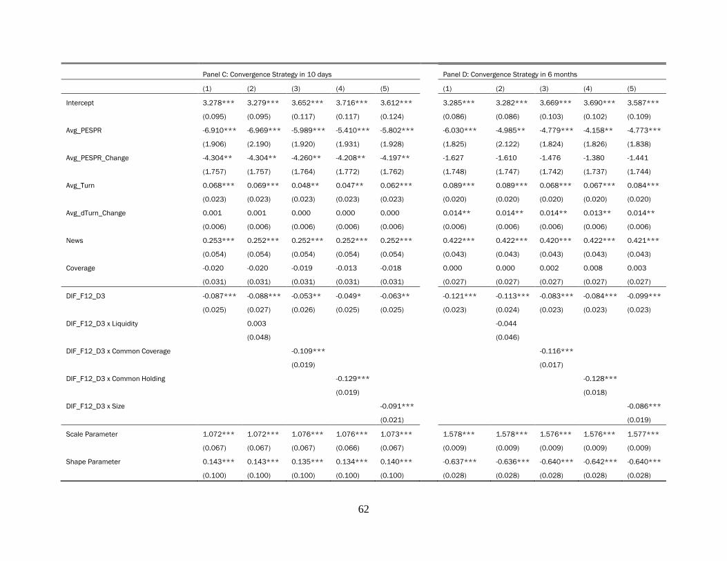
62

Panel C: Convergence Strategy in 10 days Panel D: Convergence Strategy in 6 months

(1) (2) (3) (4) (5) (1) (2) (3) (4) (5)

Intercept 3.278*** 3.279*** 3.652*** 3.716*** 3.612*** 3.285*** 3.282*** 3.669*** 3.690*** 3.587***

(0.095) (0.095) (0.117) (0.117) (0.124) (0.086) (0.086) (0.103) (0.102) (0.109)

Avg_PESPR -6.910*** -6.969*** -5.989*** -5.410*** -5.802*** -6.030*** -4.985** -4.779*** -4.158** -4.773***

(1.906) (2.190) (1.920) (1.931) (1.928) (1.825) (2.122) (1.824) (1.826) (1.838)

Avg_PESPR_Change -4.304** -4.304** -4.260** -4.208** -4.197** -1.627 -1.610 -1.476 -1.380 -1.441

(1.757) (1.757) (1.764) (1.772) (1.762) (1.748) (1.747) (1.742) (1.737) (1.744)

Avg_Turn 0.068*** 0.069*** 0.048** 0.047** 0.062*** 0.089*** 0.089*** 0.068*** 0.067*** 0.084***

(0.023) (0.023) (0.023) (0.023) (0.023) (0.020) (0.020) (0.020) (0.020) (0.020)

Avg_dTurn_Change 0.001 0.001 0.000 0.000 0.000 0.014** 0.014** 0.014** 0.013** 0.014**

(0.006) (0.006) (0.006) (0.006) (0.006) (0.006) (0.006) (0.006) (0.006) (0.006)

News 0.253*** 0.252*** 0.252*** 0.252*** 0.252*** 0.422*** 0.422*** 0.420*** 0.422*** 0.421***

(0.054) (0.054) (0.054) (0.054) (0.054) (0.043) (0.043) (0.043) (0.043) (0.043)

Coverage -0.020 -0.020 -0.019 -0.013 -0.018 0.000 0.000 0.002 0.008 0.003

(0.031) (0.031) (0.031) (0.031) (0.031) (0.027) (0.027) (0.027) (0.027) (0.027)

DIF_F12_D3 -0.087*** -0.088*** -0.053** -0.049* -0.063** -0.121*** -0.113*** -0.083*** -0.084*** -0.099***

(0.025) (0.027) (0.026) (0.025) (0.025) (0.023) (0.024) (0.023) (0.023) (0.023)

DIF_F12_D3 x Liquidity 0.003 -0.044

(0.048) (0.046)

DIF_F12_D3 x Common Coverage -0.109*** -0.116***

(0.019) (0.017)

DIF_F12_D3 x Common Holding -0.129*** -0.128***

(0.019) (0.018)

DIF_F12_D3 x Size -0.091*** -0.086***

(0.021) (0.019)

Scale Parameter 1.072*** 1.072*** 1.076*** 1.076*** 1.073*** 1.578*** 1.578*** 1.576*** 1.576*** 1.577***

(0.067) (0.067) (0.067) (0.066) (0.067) (0.009) (0.009) (0.009) (0.009) (0.009)

Shape Parameter 0.143*** 0.143*** 0.135*** 0.134*** 0.140*** -0.637*** -0.636*** -0.640*** -0.642*** -0.640***

(0.100) (0.100) (0.100) (0.100) (0.100) (0.028) (0.028) (0.028) (0.028) (0.028)

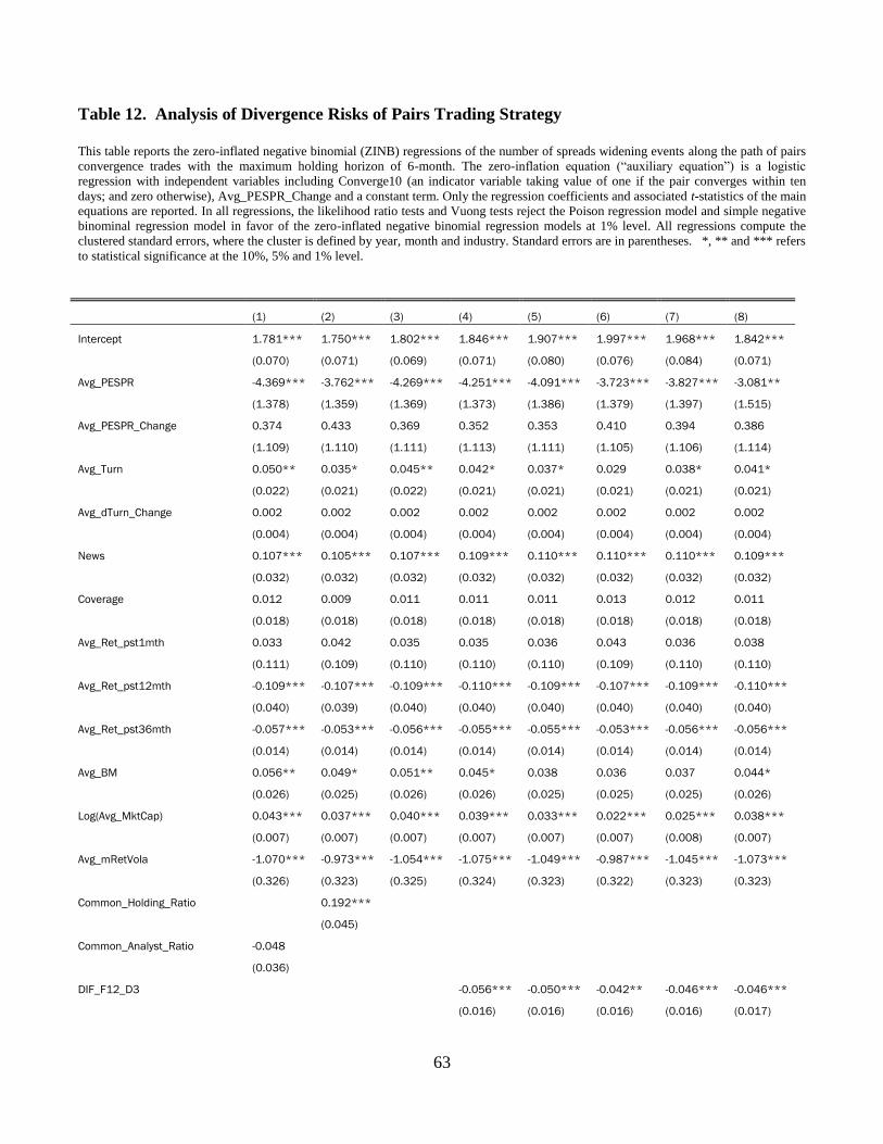
63

Table 12. Analysis of Divergence Risks of Pairs Trading Strategy

This table reports the zero-inflated negative binomial (ZINB) regressions of the number of spreads widening events along the path of pairs

convergence trades with the maximum holding horizon of 6-month. The zero-inflation equation (“auxiliary equation”) is a logistic

regression with independent variables including Converge10 (an indicator variable taking value of one if the pair converges within ten

days; and zero otherwise), Avg_PESPR_Change and a constant term. Only the regression coefficients and associated t-statistics of the main

equations are reported. In all regressions, the likelihood ratio tests and Vuong tests reject the Poison regression model and simple negative

binominal regression model in favor of the zero-inflated negative binomial regression models at 1% level. All regressions compute the

clustered standard errors, where the cluster is defined by year, month and industry. Standard errors are in parentheses. *, ** and *** refers

to statistical significance at the 10%, 5% and 1% level.

(1) (2) (3) (4) (5) (6) (7) (8)

Intercept 1.781*** 1.750*** 1.802*** 1.846*** 1.907*** 1.997*** 1.968*** 1.842***

(0.070) (0.071) (0.069) (0.071) (0.080) (0.076) (0.084) (0.071)

Avg_PESPR -4.369*** -3.762*** -4.269*** -4.251*** -4.091*** -3.723*** -3.827*** -3.081**

(1.378) (1.359) (1.369) (1.373) (1.386) (1.379) (1.397) (1.515)

Avg_PESPR_Change 0.374 0.433 0.369 0.352 0.353 0.410 0.394 0.386

(1.109) (1.110) (1.111) (1.113) (1.111) (1.105) (1.106) (1.114)

Avg_Turn 0.050** 0.035* 0.045** 0.042* 0.037* 0.029 0.038* 0.041*

(0.022) (0.021) (0.022) (0.021) (0.021) (0.021) (0.021) (0.021)

Avg_dTurn_Change 0.002 0.002 0.002 0.002 0.002 0.002 0.002 0.002

(0.004) (0.004) (0.004) (0.004) (0.004) (0.004) (0.004) (0.004)

News 0.107*** 0.105*** 0.107*** 0.109*** 0.110*** 0.110*** 0.110*** 0.109***

(0.032) (0.032) (0.032) (0.032) (0.032) (0.032) (0.032) (0.032)

Coverage 0.012 0.009 0.011 0.011 0.011 0.013 0.012 0.011

(0.018) (0.018) (0.018) (0.018) (0.018) (0.018) (0.018) (0.018)

Avg_Ret_pst1mth 0.033 0.042 0.035 0.035 0.036 0.043 0.036 0.038

(0.111) (0.109) (0.110) (0.110) (0.110) (0.109) (0.110) (0.110)

Avg_Ret_pst12mth -0.109*** -0.107*** -0.109*** -0.110*** -0.109*** -0.107*** -0.109*** -0.110***

(0.040) (0.039) (0.040) (0.040) (0.040) (0.040) (0.040) (0.040)

Avg_Ret_pst36mth -0.057*** -0.053*** -0.056*** -0.055*** -0.055*** -0.053*** -0.056*** -0.056***

(0.014) (0.014) (0.014) (0.014) (0.014) (0.014) (0.014) (0.014)

Avg_BM 0.056** 0.049* 0.051** 0.045* 0.038 0.036 0.037 0.044*

(0.026) (0.025) (0.026) (0.026) (0.025) (0.025) (0.025) (0.026)

Log(Avg_MktCap) 0.043*** 0.037*** 0.040*** 0.039*** 0.033*** 0.022*** 0.025*** 0.038***

(0.007) (0.007) (0.007) (0.007) (0.007) (0.007) (0.008) (0.007)

Avg_mRetVola -1.070*** -0.973*** -1.054*** -1.075*** -1.049*** -0.987*** -1.045*** -1.073***

(0.326) (0.323) (0.325) (0.324) (0.323) (0.322) (0.323) (0.323)

Common_Holding_Ratio 0.192***

(0.045)

Common_Analyst_Ratio -0.048

(0.036)

DIF_F12_D3 -0.056*** -0.050*** -0.042** -0.046*** -0.046***

(0.016) (0.016) (0.016) (0.016) (0.017)

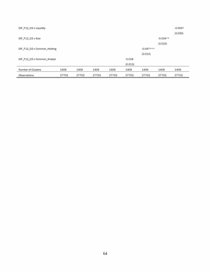
64

DIF_F12_D3 x Liquidity -0.055*

(0.030)

DIF_F12_D3 x Size -0.034**

(0.015)

DIF_F12_D3 x Common_Holding -0.047***

(0.014)

DIF_F12_D3 x Common_Analyst -0.018

(0.013)

Number of Clusters 1409 1409 1409 1409 1409 1409 1409 1409

Observations 27703 27703 27703 27703 27703 27703 27703 27703

65

Table A.1: Factor Regression of Monthly Pairs Trading Strategy Returns This table reports the factor regression of pairs trading strategy monthly returns. In Panel A, pairs are closed out by the tenth day; and in

Panel B, pairs are closed out by the end of the sixth month. MKTRF, SMB, HML, MOM and LIQ are the market factor, small-minus-big

factor, high-minus-low factor, momentum factor, and liquidity factor. In regressions (1) and (2) of each panel, the liquidity factors are the

value-weighted version and equally-weighted version of Pastor-Stambaugh liquidity factor (Pastor and Stambaugh, 2003), respectively; in

regressions (3) and (4) of each panel, the liquidity factors are the fixed-cost and variable-cost components of the spreads liquidity risk

factors constructed by Sadka (2006). Due to availability of liquidity risk factors, the sample period for regressions (1) and (2) is from

January, 1993 to December, 2004; and the sample period for regressions (3) and (4) is from January, 1993 to December, 2005.

Panel A: 10-day strategy monthly return

Panel B: 6-month strategy monthly return

(1) (2) (3) (4)

(1) (2) (3) (4)

Intercept 0.019*** 0.019*** 0.018*** 0.018***

0.008*** 0.008*** 0.008*** 0.008***

(0.001) (0.001) (0.001) (0.001)

(0.001) (0.001) (0.001) (0.001)

MKTRF 0.018 0.006 0.012 0.020

0.005 -0.001 0.002 0.004

(0.038) (0.040) (0.039) (0.042)

(0.024) (0.024) (0.023) (0.025)

SMB 0.021 0.017 0.022 0.025

0.050* 0.048 0.051* 0.051

(0.039) (0.042) (0.042) (0.041)

(0.030) (0.032) (0.031) (0.031)

HML -0.033 -0.034 -0.009 0.001

-0.013 -0.013 0.002 0.002

(0.054) (0.058) (0.055) (0.060)

(0.033) (0.034) (0.033) (0.038)

MOM -0.037 -0.046 -0.067** -0.056**

-0.077*** -0.082*** -0.092*** -0.089***

(0.029) (0.037) (0.028) (0.028)

(0.019) (0.019) (0.016) (0.018)

LIQ -0.049** -0.032 -0.536 -0.797*

-0.026 -0.017 -0.389 -0.288

(0.024) (0.036) (0.887) (0.443)

(0.017) (0.020) (0.665) (0.276)

Observations 144 144 156 156

144 144 156 156

R-Squared 0.077 0.06088 0.06117 0.09048

0.2927 0.2807 0.2831 0.2899

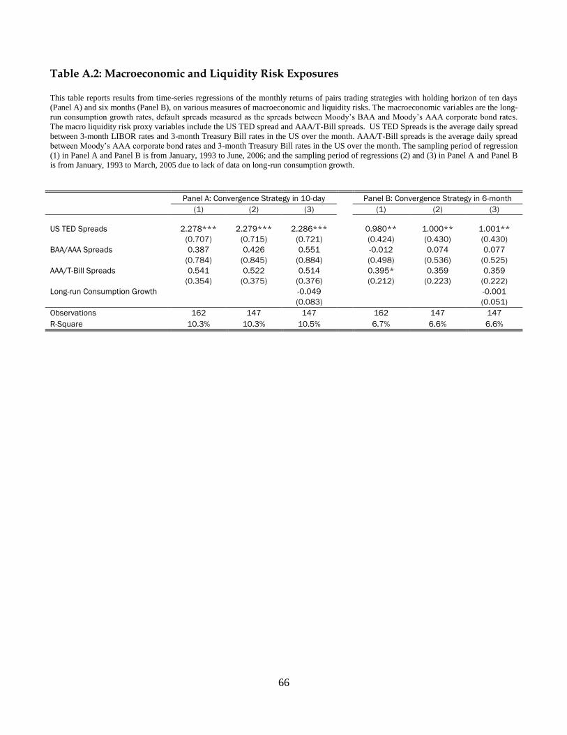
66

Table A.2: Macroeconomic and Liquidity Risk Exposures This table reports results from time-series regressions of the monthly returns of pairs trading strategies with holding horizon of ten days

(Panel A) and six months (Panel B), on various measures of macroeconomic and liquidity risks. The macroeconomic variables are the long-

run consumption growth rates, default spreads measured as the spreads between Moody’s BAA and Moody’s AAA corporate bond rates.

The macro liquidity risk proxy variables include the US TED spread and AAA/T-Bill spreads. US TED Spreads is the average daily spread

between 3-month LIBOR rates and 3-month Treasury Bill rates in the US over the month. AAA/T-Bill spreads is the average daily spread

between Moody’s AAA corporate bond rates and 3-month Treasury Bill rates in the US over the month. The sampling period of regression

(1) in Panel A and Panel B is from January, 1993 to June, 2006; and the sampling period of regressions (2) and (3) in Panel A and Panel B

is from January, 1993 to March, 2005 due to lack of data on long-run consumption growth.

Panel A: Convergence Strategy in 10-day

Panel B: Convergence Strategy in 6-month

(1) (2) (3)

(1) (2) (3)

US TED Spreads 2.278*** 2.279*** 2.286***

0.980** 1.000** 1.001**

(0.707) (0.715) (0.721)

(0.424) (0.430) (0.430)

BAA/AAA Spreads 0.387 0.426 0.551

-0.012 0.074 0.077

(0.784) (0.845) (0.884)

(0.498) (0.536) (0.525)

AAA/T-Bill Spreads 0.541 0.522 0.514

0.395* 0.359 0.359

(0.354) (0.375) (0.376)

(0.212) (0.223) (0.222)

Long-run Consumption Growth

-0.049

-0.001

(0.083) (0.051)

Observations 162 147 147

162 147 147

R-Square 10.3% 10.3% 10.5% 6.7% 6.6% 6.6%