An application of the Heckman Selection Model

to the Analysis of GIS benefits

by Chunyun Dai

Major Paper presented to the

Department of Economics of the University of Ottawa

in partial fulfillment of the requirements of the M.A. Degree

Supervisor: Professor Kathleen M. Day

Ottawa, Ontario

August 2017

i

Abstract

Previous studies have identified several characteristics that likely affect the incidence of senior

poverty. However, no research addresses the relationship between personal characteristics and the

amount of GIS benefits received, which would help to predict directly the demands placed by the

senior population on the GIS. In this paper, I expand on the existing literature by using the

Heckman two-step selection model to estimate the probability that seniors receive GIS benefits as

well as the amount of GIS benefits received, given the senior’s characteristics. The results of the

Heckman two-step estimation procedure indicate that selection bias exists. The results also show

that seniors who participate in the job market, are highly educated, live in Ontario, are non-

immigrants, and speak English have lower probabilities of receiving GIS benefits. In contrast, as

age increases, seniors are increasingly likely to receive GIS benefits regardless of the type of

household living arrangement, especially seniors who are lone parents, are living with non-

relatives only, or are living alone. The marginal effects of gender for the 65 to 69 and 70 to 74 age

groups show that men are more likely to receive GIS benefits. This result contradicts those of other

researchers. Furthermore, a senior who speaks French only has a higher probability of receiving

GIS benefits as age increases. The results of the second-stage equation modelling the amount of

annual GIS benefits received fill an existing gap in previous research. The estimates imply that the

average predicted annual amounts of GIS annual benefits, conditional on receipt of benefits, are

$5,780, $6,011, $4,590, $4,586 and $5,167 for the five age groups considered, respectively.

Individuals who had been employed at some time in the past or who have a higher level of

education receive on average smaller amounts of GIS benefits, but these effects diminish as age

increases. Immigrant status and the type of household living arrangement also affect the amount

of benefit received. Seniors who are lone parents, living alone, or immigrants receive more GIS

benefits per year, and the impacts of household living arrangements are fairly large. The marginal

effects of gender for the 65 to 69 and 70 to 74 age groups show that on average, men receive more

GIS benefits than women.

ii

Table of Contents

Abstract………………………………….…………………….………………………………...…i

1. Introduction……………………………………………….………………………………….....1

2. Background……………………………………………………………………………………..3

2.1. The Canadian retirement income system………………………………………………...…3

2.2. Canadian public pension plans and senior poverty……………………………………...….6

2.3. Sources of retirement income……………………………………………………………....7

2.4. Shortcomings of public pension plans……………………………………………………...9

2.5. Program expenditures.………………………………………...…………………..…........10

2.6. Factors affecting seniors’ income………………………………………………………....12

3. Methodology……………………………………………………………………………..........13

4. Data and its limitations………….………………………………………………………..…...15

4.1. Creation of the new variable GIS…………………………………………………..…......16

4.2. Comparison of the proportion of seniors receiving GIS benefits

in the NHS with that in other data…………………………………………………….…..18

4.3. Independent variables in the selection model and the outcome model………………..….19

5. Results and discussion…………………………………………………………………….…..22

5.1. Descriptive analysis …………………………………………………………………...….22

5.2. Heckman two-step estimation results……………………………………………….….....26

5.2.1. Selection bias issues …………………………………………………………..……..26

5.2.2. The first-stage probit model of the incidence of GIS benefits …………………..…..27

5.2.3. Comparison of the marginal effects of the corrected outcome equation

(the second-stage equation for the level of GIS benefits)

and the coefficients of the OLS equation ….……………………………..….……....32

6. Conclusion..………………………………….……………...………………...……………....38

References…………….…………………………………………………….…………………...42

iii

List of Tables

Table 1 Table1 Means and standard deviations, by age group..…………………..….….………46

Table 2 Percentage of GIS recipients, by age group and sex….………….……………….…..…48

Table 3 Sources of income by income decile group, Canadian seniors, 2010….….………….…48

Table 4 Income distribution, by age, Canadian seniors, 2010..……………………..…….…..…48

Table 5 Sources of income, by age group……….………………………………..……….….….49

Table 6 Incidence rates for GIS receipt, by household living arrangement and age group..…….49

Table 7 Incidence rates for GIS receipt, by education level and age group..………………........49

Table 8 Mills lambda, rho Wald test and number of observations, by age group…………….…50

Table 9 Estimated marginal effects of the first-stage probit model...............................................51

Table 10 Estimated marginal effects of the corrected outcome equation and

the coefficients in the OLS equation……………………………...…..………………..53

iv

List of Figures

Figure 1 Low income rates among seniors 1976 to 2009………………………………………55

Figure 2 Number of persons in low income status by age and sex (x 1,000), 1979-2009..….…55

Figure 3 Average income of seniors and non-seniors, 1976-2009…………………….……….55

1

1. Introduction

In 2016, the senior population of Canada (the number of Canadians over the age of 65) was

5,990,511, which is more than double that of the 1989 population of 2,942,304 (Statistics Canada

2016a). According to projections, the ratio of the number of people aged 20-64 to those aged 65

and over will drop from 3.8 in 2016 to 2.8 in 2025 (Office of the Superintendent of Financial

Institutions Canada, 2015). The growing senior population increases the likelihood that Canadians’

retirement income will be inadequate. Moreover, younger Canadians will feel the fiscal burden of

the decreasing ratio of non-seniors to seniors, because Canada’s public retirement income system

is a hybrid of pay-as-you-go and fully-funded public pension plans. 1

The concern stems not only from the growing senior population, but also the growing low-

income senior population. Data from Statistics Canada show that the number of low-income

seniors in 2014 was 677,000, which is double that of the 2004 population of 338,000 (Statistics

Canada 2017b.). In Canada, eligible seniors receive the Guaranteed Income Supplement (GIS),

which is financed entirely from federal government tax revenues, to help them overcome financial

difficulties. According to the 9th OAS Actuarial Report (2009), GIS expenditures increased every

year between 1992 and 2006 due to an increasing number of GIS recipients and to enhancements

to the GIS.

Notwithstanding, the level of GIS benefits is not sufficient to independently keep seniors

above the low-income cut off. For instance, the maximum payment for single people in 2010 under

the combined OAS pension, GIS and Allowance (to be presented below) is $14,075.82

1. A “pay-as-you-go” pension plan is one in which current contributions fund benefits paid in a given year. A “fully-funded”

pension plan is one in which contributions are invested, and benefits are financed by the revenues generated by the resulting

investment fund. For further information on the financing of the CPP, see Office of the Superintendent of Financial Institutions

(2014).

2

(Government of Canada 2017). The Low Income Cut-offs (LICOs) for a community with

population between 100,000 and 499,999 are $15,865 for one person, $19,308 for two persons,

and $24,043 for 3 persons in 2010 (Statistics Canada 2014, 15). While some seniors live with low-

income temporarily, poverty tends to be persistent for many others (National Advisory Council on

Aging, 2005). To explore long-term strategies for fighting poverty, which would consequently

relieve fiscal pressure on the public pension system and financial pressure on individual retirees,

researchers have analyzed the relationship between personal characteristics (among other factors)

and the incidence of senior poverty. (Finnie, Gray and Zhang, 2013; Schirle, 2013) Previous

studies have also addressed whether Canadian pension policies encourage individuals to better

prepare for their retirement. (Messacar, 2015; Veall, 2014). However, no research addresses the

relationship between personal characteristics and the amount of GIS benefits received, which

would help to predict directly the demands placed by the senior population on the GIS.

In this paper, I expand on the existing literature by using the Heckman two-stage selection

model to estimate the probability that seniors will receive GIS benefits as well as the amount of

GIS benefits received given the characteristics of seniors. This two-stage strategy is designed to

correct for sample selection bias. The paper continues in the next section with a brief discussion

of the Canadian retirement income system, followed by a discussion of how public pension plans

provide income to seniors. Also, the cost and shortcomings of the programs as well as previous

research on how personal characteristics affect GIS benefits received are reviewed. The third

section introduces the methodology used, and is followed by a description of the data used. The

fourth section analyses the results, which includes the results of a descriptive analysis, the

Heckman selection model, and a comparison of the Heckman outcome equation to an OLS model.

The conclusions are presented in the last section.

3

2. Background

2.1. The Canadian retirement income system

Canadian seniors’ retirement income comes from public and private pension plans, savings

and other assets. Old Age Security, the Guaranteed Income Supplement and the Spousal

Allowance form the first pillar in the form of a basic income guarantee for Canadian seniors.2 The

second pillar of Canada’s retirement income system is composed of the Canada Pension Plan and

the Quebec Pension Plan (CPP/QPP), which are designed “to provide contributors and their

families with a minimum level of income replacement upon the retirement, disability or death of

a wage earner.” (Employment and Social Development Canada 2017, iii). The third pillar includes

private pension plans and tax-assisted savings and investment plans. In addition, many Canadians

also have other assets for their retirement.

Old Age Security, the Guaranteed Income Supplement and the Spousal Allowance

constitute the OAS program, which is funded by general government tax revenue. The first similar

pension program began in 1927, and then was replaced by the OAS program in 1952. Old Age

Security provides a monthly flat rate to seniors, which is adjusted annually to inflation and subject

to residency requirements. The OAS pension is clawed back when annual income is above a certain

threshold, and so high-income seniors do not benefit.3

Established in 1967, the GIS provides an additional monthly payment to OAS recipients

whose income is below the GIS cut-off threshold (Young and Prisner 2007). As mentioned in

Section 1, the GIS cut-off threshold is different from a measure of low income, and is usually

2 For further information, see Young and Prisner (2007); some provinces provide income tested top-ups to the OAS and GIS.

3For further information, see http://www.esdc.gc.ca/en/cpp/oas/payments.html.

4

lower than the low income cut-off. The amount of monthly assistance is determined by an OAS

recipient’s income and marital status, and is indexed to inflation as measured by the Consumer

Price Index.4 GIS benefits are not subject to income tax.

The Spousal Allowance was established in 1975. The Allowance provides a monthly

additional income payment for an eligible spouse or common-law partner or a widowed spouse or

common-law partner aged 60 to 64 years of an OAS/GIS recipient who lives in low-income and

meets the residency requirements.5 The beneficiaries of the GIS are also provided with other

benefits such as drug insurance, etc., by the provinces and territories, some of which use receipt of

the GIS as an eligibility criterion. According to Employment and Social Development Canada

(2017), “in 2014-15, 5.6 million Canadians received almost $44.1 billion in OAS benefits and 1.7

million Canadians received almost $10.1 billion in GIS benefits.”

The CPP was introduced in 1965 and came into force in 1966 (Young and Prisner 2007).

The CPP has adapted to meet the needs of Canadians. Before 1997, the CPP was a pay-as-you-go

system;6 since 1998, it has become a hybrid of pay-as-you-go and fully-funded public pension

plans. 7 This change improved the financial sustainability of the CPP and “fairness across

generations” (Government of Canada 2015, 12). Funding of the CPP comes from mandatory

contributions by employees, their employers and the self-employed, as well as revenue earned on

the CPP surplus investments. CPP benefits include CPP retirement pensions, CPP survivor benefits

4 Income for calculating GIS benefit excludes the OAS pension and the first $3,500 of employment income. For further information,

see https://www.canada.ca/en/services/benefits/publicpensions/cpp/old-age-security/guaranteed-income-supplement/benefit-

amount.html.

5 The residency requirement is that the individual must have lived in Canada for at least ten years since the age of 18. For further

information, see https://www.canada.ca/en/services/benefits/publicpensions/cpp/old-age-security/eligibility.html

6 Pay-as-you-go social security can make all consumers better off if the population grows at a sufficiently high rate.

7 For further information on the nature of “a hybrid of pay-as-you-go and fully-funded public pension plans”, see Office of the

Superintendent of Financial Institutions (2014).

5

and CPP disability benefits to contributors and their families. The benefits are based on

contributions made during the contributors’ working years and the age at which benefits are first

received. They are intended to replace up to 25 percent of average pensionable pre-retirement

earnings (Department of Finance Canada 2010). The CPP retirement pension is a monthly taxable

benefit for contributors who are at least 60 years old. The CPP survivor benefits provide payments

to a surviving spouse or common-law partner and dependent children. They include a one-time

death benefit, a monthly payment to the surviving spouse or common-law partner, and a monthly

benefit paid to the dependent children. The CPP disability pension provides support to contributors

and their dependent children when they are prevented from working due to disability.

The third pillar consists of employer-sponsored pension plans and tax-assisted personal

retirement savings. Employer-sponsored pension plans are provided by employers on a voluntary

basis. Employers and/or employees are responsible for contributing to the plans. In general, there

are two designs: defined benefit plans promise a pension benefit based on a formula set out in the

pension plan; and defined contribution plans provide retirement income based on accumulated

contributions and investment returns. Tax assisted savings provide retirement saving opportunities

through Registered Retirement Savings Plans (RRSPs), Pooled Registered Pension Plans (PRPPs),

and Tax Free Savings Accounts (TFSAs) to supplement senior retirement income. (Canada

Revenue Agency, 2017).8

8According to Canada Revenue Agency (2016c) and Canada Revenue Agency (2016d), for Registered Retirement

Savings Plans (RRSPs) and Pooled Registered Pension Plans (PRPPs), contributions and investment earnings are tax

free until withdrawn. According to Canada Revenue Agency (2016b), the TFSAs are not established specifically to

generate retirement income but “Any amount contributed as well as any income earned in the account is generally

tax-free, even when it is withdrawn.” For further information, see http://www.cra-arc.gc.ca/tx/rgstrd/rpp-rpa/fq-

eng.html; http://www.cra-arc.gc.ca/tx/ndvdls/tpcs/prpp-rpac/menu-eng.html; http://www.cra-

arc.gc.ca/tx/ndvdls/tpcs/tfsa-celi/mpct-eng.html

6

In addition, many Canadians also have other assets such as investment income, interest and

capital gains, sales of property, etc., for their retirement.

2.2. Canadian public pension plans and senior poverty

As shown in Figure 1, the senior low-income rate in Canada displays a declining trend

from 1976 to 2007 using the Low-income Cut-offs (LICOs) (Murphy, Zhang and Dionne 2012).

However, this trend may not accurately reflect the standard of living of seniors. According to

Shillington (2016), since the LICOs are based on 1992 expenditure data, the LICO does not reflect

current consumption patterns. Using the Low-income Measure-based thresholds (LIMs), the

percentage of seniors with low income displays a declining trend from 33.1% in 1977 to 3.7% in

1995; then the low-income rate displays an increasing trend from 1996 to the present.9 This trend

is consistent with the number of seniors in low income (Figure 2).

The decline in poverty rates from 1976 through 1995 could be due to the maturation of the

CPP and QPP. As mentioned in section 2.1, the CPP and QPP were introduced in 1965 and were

implemented in 1966, providing full benefits after 10 years of contributions. In 1976, the first

contributors receiving full CPP and QPP benefits turned 65, and the CPP and QPP became major

forces in reducing the number of low income seniors over the 1980s (Myles 2000). OAS/GIS

benefits have also contributed to the decline in low income seniors. As mentioned in Section 2.1,

OAS recipients with little or no other income began to receive an additional monthly payment in

the form of GIS benefits in 1967 to ensure their incomes did not fall below a specific threshold.

9 For further information on how low income thresholds are constructed, see Statistics Canada (2016b)

7

Meanwhile, OAS pension amounts also increased during this period. For a single person, the total

annual payment of OAS and GIS benefits increased from $1,260 in 1967 to $10,426 in 1995.10

The increase in the low-income rate from 1996 to 2007 indicates that seniors’ incomes did

not grow as quickly as those of the other Canadians, which may be due to slower growth in

government transfers to seniors (Murphy et al. 2012).11 After comparing seniors’ median income

and the GIS level from 1984 through 2011, Shillington (2016, 10) reaches a similar finding: “The

median income of seniors (singles and couples) has increased by about 45 per cent, after adjusting

for inflation. In contrast, the OAS/GIS guarantee levels have increased by about 7 per cent for

senior couples and 15 per cent for single seniors.” Furthermore, the influence of CPP and QPP as

well as OAS/GIS in reducing low-income declined due to policy changes. As Myles (2000, 13)

points out, for seniors “income taxes rose from about 10% of total income in 1980 to almost 16%

by 1995,” which included the claw back rule of OAS benefit starting in 1989.

2.3. Sources of retirement income

Previous research indicates that the Canadian pension system is an important source of

retirement income for an increasing number of seniors. The share of each source in seniors’ income

varies among income groups. Using data from Statistics Canada’s Longitudinal Administrative

Database, LaRochelle-Côté, Myles and Picot (2008) selected a cohort of workers who were aged

from 54 to 56 in 1983 and tracked their incomes over twenty years. They found that retirement

income sources varied among income distribution quintiles. For instance, when individuals in the

bottom quintile in 1983 retired in 1996, public pension plans including CPP and QPP benefits and

10 Author’s calculations based on data from “Maximum Monthly Amounts for The Old Age Security Program, by Type of Benefit

and Quarter from 1952 to 2017” (Government of Canada 2017).

11 See Figure 3 of Murphy et al. (2012).

8

the OAS and GIS were their main source of income, jointly accounting for 53.1% of retirement

income before taxes, while private pensions and RRSPs accounted for 16.7% of retirement income

before taxes. Among individuals in the middle quintile, 39.4% of retirement income before taxes

was derived from CPP/QPP benefits and the OAS and GIS, and 32.4% of retirement income before

taxes was from private pensions and RRSPs. In the top quintile, CPP/QPP, OAS and GIS

accounted for 18.1% of retirement income before taxes, and private pensions and RRSPs

accounted for 29.6% of retirement income before taxes.12 The share of public pension plans of

retirement income declined from the bottom quintile to the top quintile. This is a progressive

income redistribution pattern.

In response to the objectives of the OAS program, Human Resources and Skills

Development Canada (2012a) examined the importance of the OAS pension, the GIS and the

Allowances in contributing to the reduction of low income among seniors and the low-income gap.

Examining the difference in income situations with and without the OAS program, the analysis

indicated that the OAS program cannot eliminate poverty on its own, but can lower the incidence

of low income. For instance, according to analysis derived from the Longitudinal Administrative

Database (LAD), in 2006 the incidence of low income before tax was 26.7 percentage points lower

for individual seniors than it would have been in the absence of the OAS program. The report also

examined how much money was needed to eliminate the low-income gap, which it defined as “the

aggregate dollar amount necessary to elevate all seniors up to the low-income benchmark” (Human

Resources and Skills Development Canada 2012a, 26). It concluded that the OAS program led to

“a 79 percent reduction of the low-income gap (before-tax) for single seniors in 2001, and an 82

percent reduction of the low-income gap (before-tax) for families with one senior member in 2001”

12 These numbers were derived from Table 3, Table 4, and Table 5 of LaRochelle-Côté et al. (2008).

9

(Human Resources and Skills Development Canada 2012a, 27). Overall, even if the OAS program

has not eliminated poverty among seniors, it has been successful in reducing the incidence of low

income during retirement.

2.4 Shortcomings of public pension plans

Canadian pension policies encourage individuals, their employers and governments to

share the responsibility for maintaining their standard of living in retirement. A good example is

the third pillar consisting of tax-assisted personal retirement savings and employer sponsored-

pension plans for retirement savings. By providing tax advantages for RRSPs and employer

pension plans, these vehicles encourage Canadians to save for their retirement, so as to decrease

the likelihood of seniors living in low-income. However, researchers have found that employer-

sponsored pension plans, which are pensions or retirement savings plans offered by employers as

a benefit to their employees, are affected by the contribution rate of the CPP. Regarding the

relationship between employer-sponsored pension plans and tax-assisted personal retirement

savings, employer-sponsored pension plans “partially crowd out contributions into registered

retirement savings plans----by approximately $0.50 per $1.00” (Messacar 2015, 5).

In addition, certain groups may not benefit from these various savings and work incentive

policies. For instance, there are a lot of workers who simply cannot afford to save for retirement.

When people with low income put their money into a RRSP, they may not save on income taxes

due to their low income. By contrast, if they are entitled to GIS benefits when retired, since GIS

benefits are income tested benefits, GIS benefits would be reduced due to the GIS clawback if they

earn income from any other source, including employment, pensions, etc.:

GIS benefits: reduced at the rate of 50 cents for every dollar of income received on top of

the OAS/GIS pension and the first $3,500 of employment income. The reduction is 25

10

cents for every dollar on top of the OAS and GIS benefits and the first $2,000 of income

($4,000 for couples) for the GIS top-up. (Employment and Social Development Canada

2017, 29).

Thus, according to these rules, GIS benefits would be reduced by $500 for each $1,000 of RRSP

income due to the GIS clawback of 50 percent. Therefore, if the combination of the interest rate

and the marginal personal income tax rate at the time of contribution is lower than the GIS

clawback rate of 50 percent, the individual would not benefit from contributing to an RRSP

(National Advisory Council on Aging 2005). Veall (2014) reports that a range of 15 percent to 30

percent of recipients of RRSPs/ RPPs were subject to a GIS clawback when they cashed out their

RRSPs/RPPs after they retired. Furthermore, Veall also states that three fifths of RRSP recipients

would lose at least $1,000 yearly due to the GIS clawback of RRSP withdrawals. The same issue

would arise if seniors’ income came from registered pension plans.

Furthermore, other policies, such as enhancing the CPP, would also not help some groups.

For example, policies that enhance the CPP will not help unattached seniors who never worked

accumulate money for retirement, since the CPP is a work-related investment. Also, since

allowances for spouses would not provide benefits to single seniors, single seniors would not

receive any benefit from this policy change either (Cross 2014).

2.5 Program expenditures

To address these particular financial circumstances, one option is to create alternative

saving mechanisms where contributions to savings would be from after-tax income, but the

withdrawals are tax-free during retirement (National Advisory Council on Aging, 2005). Such a

savings vehicle would be the opposite of investing in an RRSP, and might encourage low income

earners to save for retirement. In 2009, the Canadian government launched the Tax-Free Saving

11

Account (TFSA) program. Although the TFSA was not created specifically to generate retirement

income, earnings in the account and withdrawals are tax-free.13 Another recommendation is to

provide a small exemption for RRSP and RRIF income when calculating income for the GIS (Veall

2014). However, these suggestions may raise the fiscal costs of the GIS. According to Veall’s

calculations, there are 180,000 seniors receiving both GIS and RRSP or RRIF income. Thus, an

exemption of just $1,000 provided to each beneficiary would increase federal government

expenditure annually by $90 million. As Veall (2014, 388) stated: “There is a good argument for

the latter reform, but it would increase the cost to the treasury.”

In fact, even if no new cost is added, OAS costs would still increase every year. Data from

the 9th OAS Actuarial Report (2009) show that from 1992 to 2007, expenditures from the OAS,

GIS, and the Spousal Allowance increased every year. In 1992, $14,292 million of OAS was paid

to beneficiaries, rising to $24,711 million in 2007, while GIS payments rose from $4,227 million

in 1992 to $7,346 million in 2007. The Spousal Allowance increased from about $438 million in

1992 to $513 million in 2007. This increasing trend can be explained by the increase in the number

of seniors over time and the indexation of benefits to inflation. In addition, administrative expenses

also display an increasing trend over time, from $77 million in 1992 to $112 million in 2007.

Furthermore, the number of beneficiaries of the program is expected to double between 2010 and

2030.14 The increasing expenditures of the OAS program have created financial pressure on the

federal government over time, since the federal government is responsible for funding the program.

For the fiscal year ending on March 31, 2014, 15 cents of each tax dollar were spent on Old Age

13 For further information, see http://www.cra-arc.gc.ca/tx/ndvdls/tpcs/tfsa-celi/menu-eng.html.

14 These values are from Table 7 of Office of the Superintendent of Financial Institutions Canada (2009, 27)

12

Security (OAS), Guaranteed Income Supplement (GIS), and Allowance for Spouses (Department

of Finance Canada, 2014).

2.6 Factors affecting seniors’ income

Since OAS benefit payments have increased government expenditures, which may lead to

other economic consequences, researchers are looking for the causes of low income, in hopes of

eliminating the roots of poverty. Previous studies have confirmed that some personal

characteristics are associated with a higher risk of low income. Using the Longitudinal

Administrative Data (LAD) file from 1982 to 2008, Finnie, Gray, and Zhang (2013 s76) estimate,

using a linear probability model, that the incidence rate for receiving GIS benefits among single

female seniors “is 8 percentage points higher than that of single men,” holding all other factors

constant. Furthermore, the incidence rate for receiving GIS benefits among female seniors

increases as their age increases (Uppal, Wannell and Imbeau, 2009). In terms of regional factors,

Ontario has the lowest incidence rate (Finnie et al., 2013).

Besides the effects mentioned above, other characteristics come into play as well. Schirle

(2013) conducts a decomposition analysis that examines how the characteristics of seniors

contribute to the likelihood of living in poverty over time. According to Schirle’s study, although

the results were different for different datasets and different measures of low income, variables

related to education level, age, birthplace, family composition and the location of residence are all

factors that can predict the likelihood of poverty among seniors.15

15 Schirle’s data included the Survey of Consumer Finances and Survey of Labour and Income Dynamics (1977-79, 1994-96, and

2006-08).

13

3. Methodology

In this paper, I want to estimate the effect of various factors on the amount of GIS benefits

received. A simple linear regression model for the amount of GIS benefits received could be

written as

𝑦𝑖 = 𝐱𝑖′𝛽 + 𝜀𝑖, (1)

where yi is the amount of GIS benefits received, xi represents a vector of explanatory variables (to

be discussed in the next section), and εi is an error term that is assumed to be independently and

identically normally distributed with a zero mean.

A potential problem with OLS estimation of this equation is that the amount of GIS benefits

received depends on whether or not the senior meets the residency and annual income requirements,

which means that the amount of GIS benefits received is a censored random variable.16 Many

individuals receive no GIS benefits. Thus, the assumption that the dependent variable is normally

distributed is violated. Furthermore, if equation (1) is estimated using only the observations for

which yi ≠ 0, the parameter estimates will be biased. To see this, let the equation that determines

whether an individual receives GIS benefits be

𝑧𝑖 = 𝒘𝑖

′ 𝛾 + 𝑢𝑖, (2)

where zi is an unobservable index of eligibility for GIS, wi is a vector of seniors’ characteristics,

and the random error ui is assumed to have a standard normal distribution. If zi > 0, individual i is

eligible to receive GIS benefits. Then, the sample selection rule is that yi is observed only when zi

is greater than zero. The expected GIS benefit, given that the individual is eligible, is thus

16 Note that the individual must also be aged 65 or over to receive GIS benefits.

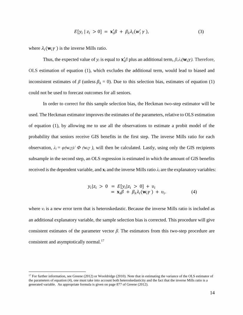
14

𝐸[𝑦𝑖 | 𝑧𝑖 > 0] = 𝐱𝑖′𝛽 + 𝛽𝜆𝜆𝑖(𝒘𝑖

′ 𝛾 ), (3)

where 𝜆𝑖(𝐰𝑖𝛾 ) is the inverse Mills ratio.

Thus, the expected value of yi is equal to 𝐱𝑖′β plus an additional term, βλλi(𝐰𝑖𝛾). Therefore,

OLS estimation of equation (1), which excludes the additional term, would lead to biased and

inconsistent estimates of β (unless 𝛽λ = 0). Due to this selection bias, estimates of equation (1)

could not be used to forecast outcomes for all seniors.

In order to correct for this sample selection bias, the Heckman two-step estimator will be

used. The Heckman estimator improves the estimates of the parameters, relative to OLS estimation

of equation (1), by allowing me to use all the observations to estimate a probit model of the

probability that seniors receive GIS benefits in the first step. The inverse Mills ratio for each

observation, λi = φ(wiγ)/ Ф (wiγ ), will then be calculated. Lastly, using only the GIS recipients

subsample in the second step, an OLS regression is estimated in which the amount of GIS benefits

received is the dependent variable, and xi and the inverse Mills ratio λi are the explanatory variables:

𝑦𝑖|𝑧𝑖 > 0 = 𝐸[𝑦𝑖|𝑧𝑖 > 0] + ʋ𝑖

= 𝐱𝒊𝛽 + 𝛽λ𝜆𝑖(𝐰𝑖𝛾 ) + ʋ𝑖. (4)

where νi is a new error termthat is heteroskedastic. Because the inverse Mills ratio is included as

an additional explanatory variable, the sample selection bias is corrected. This procedure will give

consistent estimates of the parameter vector β. The estimators from this two-step procedure are

consistent and asymptotically normal.17

17 For further information, see Greene (2012) or Wooldridge (2010). Note that in estimating the variance of the OLS estimator of

the parameters of equation (4), one must take into account both heteroskedasticity and the fact that the inverse Mills ratio is a

generated variable. An appropriate formula is given on page 877 of Greene (2012).

15

According to Cameron and Trivedi (2005, 551), the parameters of this two-equation sample

selection model are identified even in the case where xi = wi. However, in practice they may not

be, due to multicollinearity between the inverse Mills ratio and the other explanatory variables, if

xi = wi. To avoid this problem, in my empirical analysis I will exclude from xi some of the variables

that are included in wi.

To test for selectivity bias, I examine the estimate of βλ. If I cannot reject the null hypothesis

that βλ = 0, then sample selection does not result in significant bias, and so applying OLS to the

outcome equation based on the selected sample without including the inverse Mills ratio is

appropriate. Otherwise, sample selection causes significant bias, and the inverse Mills ratio should

be included when the GIS benefits model is estimated.

4. Data and its Limitations

The data source is the Individuals File of the 2011 National Household Survey (NHS).

According to Statistics Canada (2017, 5), “the NHS covers all persons who usually live in Canada,

in the provinces and the territories. It includes persons who live on Indian reserves and in other

Indian settlements, permanent residents, non-permanent residents such as refugee claimants,

holders of work or study permits, and members of their families living with them.” In this paper,

the sample is restricted to individuals who are aged 65 and over. The NHS contains 117,741 seniors,

which is 13.27 % of the total sample. The distribution of observations among age groups, the

percentage of the total senior population, and the percentage of the entire sample are as follows:

60 to 69 years 39,413 33.47% 4.47% 18

70 to 74 years 28,978 24.61% 3.28%

75 to 79 years 22,629 19.22% 2.56%

80 to 84 years 15,713 13.35% 1.78%

85 years and over 11,008 9.35% 1.25%

18 The entire sample in the dataset: 882,287

16

According to the 2011 NHS, 92.04% of seniors received OAS/GIS benefits, and 7.96% of seniors

did not receive OAS/GIS benefits.

4.1 Creation of the new variable GIS

Although the NHS Public Use Microdata File (PUMF) contains detailed information on

income from different sources, it combines OAS and GIS payments in one variable. However,

OAS eligibility depends only on the individual’s age and a residency requirement, while GIS

eligibility depends on income as well. Thus receipt of GIS benefits is an indicator of senior poverty.

To generate a measure of GIS benefits, OAS payments must be removed from the variable as it

appears in the NHS.

In the NHS, the unit of analysis is the individual, for whom certain characteristics are

provided. Furthermore, periods of residence, legal status as well as income have already been

factored in when determining eligibility for OAS program benefits by administrative processing

officers; therefore, the values of the combined variable OASGI are the actual total amounts seniors

received from OAS and GIS in 2010. Thus, the effect of income on GIS entitlements (either

individuals’ income or their family income) has already been considered before generating the GIS

variable.

In 2010, the maximum basic OAS pension for individuals who have lived in Canada for at

least 40 years after age 18 is as follows:

January to March: $516.96

April to June: $516.96

July to September: $518.51

October to December: $521.62

Total full OAS benefit in 2010 was $6,222.15.

17

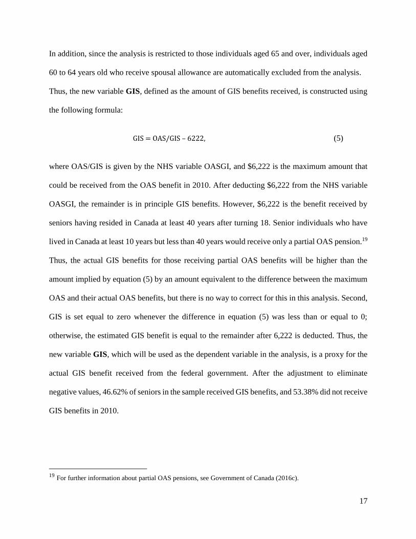
In addition, since the analysis is restricted to those individuals aged 65 and over, individuals aged

60 to 64 years old who receive spousal allowance are automatically excluded from the analysis.

Thus, the new variable GIS, defined as the amount of GIS benefits received, is constructed using

the following formula:

GIS = OAS/GIS – 6222, (5)

where OAS/GIS is given by the NHS variable OASGI, and $6,222 is the maximum amount that

could be received from the OAS benefit in 2010. After deducting $6,222 from the NHS variable

OASGI, the remainder is in principle GIS benefits. However, $6,222 is the benefit received by

seniors having resided in Canada at least 40 years after turning 18. Senior individuals who have

lived in Canada at least 10 years but less than 40 years would receive only a partial OAS pension.19

Thus, the actual GIS benefits for those receiving partial OAS benefits will be higher than the

amount implied by equation (5) by an amount equivalent to the difference between the maximum

OAS and their actual OAS benefits, but there is no way to correct for this in this analysis. Second,

GIS is set equal to zero whenever the difference in equation (5) was less than or equal to 0;

otherwise, the estimated GIS benefit is equal to the remainder after 6,222 is deducted. Thus, the

new variable GIS, which will be used as the dependent variable in the analysis, is a proxy for the

actual GIS benefit received from the federal government. After the adjustment to eliminate

negative values, 46.62% of seniors in the sample received GIS benefits, and 53.38% did not receive

GIS benefits in 2010.

19 For further information about partial OAS pensions, see Government of Canada (2016c).

18

4.2. Comparison of the proportion of seniors receiving GIS benefits in the NHS with that in other

dataset

In order to put the analysis in perspective, the maximum OAS and GIS benefits received,

and the proportions of seniors who received GIS benefits in 2010 are compared between the NHS

and the Survey of Labour and Income Dynamics, 2011 [Canada]: Person File (SLID). In the NHS,

the maximum combined OAS and GIS received is $21,200, while the maximum combined OAS

and GIS benefit amounts are $20,500 in the SLID. Though not identical, these two numbers are

similar. The estimated proportion of seniors who received GIS benefits is 46.62% in the NHS, and

35.86% in the SLID. The proportion of seniors who received GIS benefits seems be higher in the

NHS according to the new variable GIS.

While the two datasets cannot provide the answer as to why the proportions of seniors who

received GIS benefits are different, possible causes are proposed. First, the sample NHS

respondents may be different from the respondents in the SLID. The SLID has a smaller sample

size, so different samples would produce different estimates. The NHS contains 117,741 seniors,

while the SLID contains only 3,628. Second, the datasets are from self-administered surveys, and

the calculation of received OAS and GIS benefits could be complicated for some seniors, which

may cause a difference between actual amounts of GIS received and the amount reported.

Furthermore, since both datasets are self-administered surveys, they cannot be more

accurate than data obtained directly from the Canada Revenue Agency or Employment and Social

Development Canada (These data are restricted, so I cannot access these datasets.). Nevertheless,

it is possible that the high proportion of GIS recipients calculated with the NHS data is accurate.

The report of the Organisation for Economic Co-operation and Development (OECD) (2013, 1)

supports this possibility, stating that during the crisis period from 2007 to 2010, the poverty rates

for seniors increased in Canada: “while old-age poverty fell in 20 OECD countries between 2007

19

and 2010, old-age poverty in Canada increased by about 2 percentage points over the same period.”

Based on the reasons stated above, and the fact that the actual GIS benefits for those receiving

partial OAS benefits will be higher than the amount implied by the calculations, I think that the

new generated variable GIS is a reasonably good indicator of seniors’ poverty in 2010. (Recall

that since GIS benefits are means-tested, receipt of GIS benefits indicates that the individual’s

non-GIS income was low.)

4.3. Independent variables in the selection model and the outcome model

In the selection equation, the independent variables refer to the date last worked for pay or

in self-employment, household living arrangements, immigrant status, sex, education, province or

territory of residence in 2010, and official language. These variables are selected to determine the

likelihood that seniors receive GIS benefits. In the outcome equation, the independent variables

also refer to the date last worked for pay or in self-employment, household living arrangements,

immigrant status, sex, education and the inverse Mills ratio λi. These variables are selected to

model the amount of GIS benefits received. Furthermore, since all the independent variables

except the inverse Mills ratio are categorical variables, to analyze the difference between

categories, each category of the variable will be treated as a separate covariate, with the first

category of the respective variable selected as its base. Thus, the coefficients reflect the deviation

in the dependent variable (predicted probabilities or amounts) for that particular category relative

to the reference category. In addition, as noted in section 3, if all the variables in the selection

equation are also included in the outcome equation, a multicollinearity problem may exist in the

outcome equation that makes it difficult to identify its parameter estimates. As a result, the

20

estimated coefficients of the outcome equation may be imprecise. Thus, the variables related to

place of residence in 2010 and official language are not included in the outcome equation.

The date last worked for pay or in self-employment has four categories: last worked before

2010, last worked in 2010, last worked in 2011, and never worked. The results would disclose how

labour force participation in the specified year affects the probability of receiving GIS and the

amount of GIS. Household living arrangements are also important, since they not only reflect

marital status, but also family composition, which may affect both income level and the

qualification threshold for GIS benefits. Household living arrangements include the categories of

married or common-law without children, married or common-law with children, lone parent,

child of a couple, child of a lone parent (these two categories do not seem relevant for the

population of seniors, but in fact, there is information on these two categories for certain age groups

in the data set), person living alone, person living with non-relatives only, and person not in a

census family but living with other relatives. The categories for the immigration status dummies

are non-immigrants, immigrants, and non-permanent residents. The results will disclose whether

immigration status affects the ability of seniors to accumulate financial assets; immigrants may be

at risk of having an inadequate retirement income.

Moreover, since receipt of GIS benefits depends only on seniors’ incomes and the

residency requirement, gender should not be related to whether or not seniors receive the GIS.

However, if there is inequity in earnings or in other types of income between men and women, it

might indirectly affect seniors’ retirement incomes. Thus, the differences in the probability of

receiving GIS and the amount of GIS benefits received between males and females will also be

discussed.

21

Education level is recoded into the categories of no certificate, diploma or degree; high

school diploma; trades or Registered Apprenticeship certificate; college, CEGEP, or other non-

university certificate; university; degree in medicine, dentistry, veterinary medicine or optometry;

master's degree; and earned doctorate degree. It is well-known that education has been identified

as a determinant of income, and therefore is likely to affect receipt of GIS benefits.

Province or territory of residence in 2010 includes Newfoundland and Labrador, Prince

Edward Island, Nova Scotia, New Brunswick, Quebec, Ontario, Manitoba, Saskatchewan, Alberta,

British Columbia, and Northern Canada. The place of residence is included because various local

economic characteristics might affect individuals’ incomes, which ultimately determine whether

or not the senior receives the GIS, and what level of benefit is. Official language is classified into

English only, French only, both English and French, and neither English nor French. Since

language skills impact the likelihood of people participating in the job market as well as their

income, this factor also is included in the models.

Table 1 lists the means and standard deviations of all the dummy explanatory variables

disaggregated by age group. Since all the independent variables used in the analysis are categorical

variables, computing means and standard deviations of the original categorical variables does not

make sense. However, it does make sense to do so for the individual dummy variables for each

category, as the mean of a dummy variable discloses the proportion of individuals in the sample

who fall into corresponding category. For instance, the mean of immigrants in the 65 to 69 age

group is 0.2869, which indicates that 28.69% of individuals in this subsample fall into that category.

Furthermore, Table 1 helps to identify atypical cases where the number of individuals constitutes

a very small percentage of the sample or is non-existent. For instance, the number of individuals

in the categories of lone parent, child of a couple, and child of a lone parent are 1158, 2, and 97 in

22

the 65 to 69 age group. Thus 2.94%, 0.01%, and 0.25% of individuals in this age group fall into

the corresponding categories. In the 85 years and over age group, the number of individuals in the

categories of lone parent, child of a couple, child of a lone parent are 1119, 0, and 0. Thus 10.17%,

0.00%, and 0.00% of individuals in this age group fall into the corresponding categories.

5. Results and discussion

In this section, I begin with a descriptive analysis of seniors’ incomes in 2010. The

Heckman two-step selection model is then used to examine the probability of receiving GIS

benefits and the amount of GIS benefits received, by age group. I analyze the effects of the

independent variables by age group because I find that there are common patterns among those in

the same age group.

5.1. Descriptive analysis

In 2010, 45.99% of seniors (all ages combined) received GIS benefits. Table 2 lists the

percentage of female GIS recipients and male GIS recipients in each age group. The female column

is calculated as follows: (number of female seniors aged 65-69 who receive GIS/total number of

seniors aged 65-69 who received GIS) *100, and the male column is calculated in the same fashion.

Thus, I can compare the proportions by gender within each age group. The patterns are different

for men and women. While the percentage of female GIS recipients out of the total population of

the age group clearly increases with age, the pattern is not clear for men. In the 65 to 69 age group,

women who receive GIS benefits account for 19.28% of seniors in that age group. In the 85 years

and over age group, female GIS recipients account for 41.61% seniors in that age group, which is

more than double than that of the 65 to 69 age group. For men between the ages of 65 and 79, the

23

data show an increasing trend from 15.75% in the 65 to 69 age group to 21.14% in the 75 to 79

years age group. Then the table shows a decreasing trend for men aged 80 and above. In the 85

years and over age group, men who receive GIS benefits constitute 17.23% of seniors in that age

group. The differences across age groups are thus not big for men.

Overall, the percentages receiving GIS benefits in each age group increase as age increases

when gender effects are ignored. As age increases, more and more seniors claim and qualify for

GIS benefits. In the 65 to 69 age group, 35.03% of seniors received GIS benefits, while 58.84%

of seniors aged 85 and over rely on GIS benefits. When gender effects are considered, it is clear

that the incidence trends are driven by women.

Table 3 reveals seniors’ sources of income by income level. OAS/GIS benefits are a critical

component of seniors’ incomes for the lower income strata. For the lowest (first) decile, OAS/GIS

benefits are the most important source of income, constituting 65.57% of total income. In the

second decile, OAS/GIS benefits represent 60.34% of total income. On the other hand, higher-

income seniors have more diverse income sources. For instance, among individuals in the ninth

and highest deciles, OAS/GIS benefits account for 10.40% and 3.13% of total income, respectively.

Employment income and private pension income are relatively more important for these deciles.

Employment income and private pensions account for 22.99% and 41.60% of total income

respectively in the ninth decile. In the highest decile, they account for 43.31% and 23.45% of

income, respectively.

Table 4 presents the distribution of income within each senior age group. In all age groups,

seniors are most likely to fall in the second income decile, followed by the third decile, as these

two deciles account for the largest shares within each age group. In general, seniors are

concentrated in the second to the fifth income deciles. As age increases from 65 to 84, the

24

percentages of seniors in the second and third deciles increase. Then the percentage decreases

slightly in the third decile for the 85 years and over age group. More importantly, as age increases,

fewer seniors remain in the highest decile, with a similar downward trend apparent from the fifth

decile to the highest. More specifically, only 5.54% of seniors in the 85 years and over age group

are in the highest decile, which is about half of the 9.17% of seniors in the highest decile in the 65-

69 years age group.

Furthermore, the importance of different income sources varies according to seniors’ age

(Table 5). For individuals from 65 to 69 years old, employment income accounts for 32.52% of

total income, while OAS/GIS benefits account for 15.74%, CPP/QPP benefits for 15.12%,

investment gains for 9.34%, and private retirement pensions for 27.27%. For seniors aged 85 and

over, employment income accounts for only 1.56% of total income, while OAS/GIS benefits

account for 28.02%, CPP/QPP benefits for 21.73%, investment gains for 16.35%, and retirement

pensions account for 32.34%. Thus as age increases, private pensions eventually become the main

source of retirement income, followed by OAS and GIS. Overall, the shares of CPP/QPP,

OAS/GIS, investment income, and retirement income display an upward trend with age, while the

share of employment income in total retirement income decreases with age.

The remainder of this section looks at the characteristics of GIS recipients. The data in

Table 6 show that as age increases, seniors show an increasing need for financial assistance

regardless of the type of household living arrangement. For couples with children, or for seniors

who are lone parents, the trend is much more prominent; although these are not typical cases at all,

they are the groups that rely most heavily on GIS benefits In 2010, the percentage of lone parents

receiving GIS jumped to 65.36% within the age group of 70 to 74 years, as compared to 49.74%

for the age group of 65 to 69 years. Furthermore, the data reveal that unattached seniors need more

25

assistance as they become older. For example, 65.18% of seniors living with non-relatives receive

GIS in the age group 70 to 74 years, compared to 48.13% of seniors in the category 65 to 68 years.

Table 7 presents the percentage of senior receiving GIS by education level for each age

group. The table suggests that education plays an important role in determining seniors’ retirement

incomes. As the level of education increases, fewer and fewer seniors rely on GIS. Another

interesting pattern is that in each educational attainment category, the incidence rate for GIS

increases as age increases. This relationship between education and seniors’ incomes is obvious

among younger seniors as well as those who are 85 years and over (These sample sizes are small.).

For instance, in the category “earned doctorate degree,” 14.95% of seniors aged 65 to 69 years rely

on GIS benefits; the percentage increases to 36.92% of those 85 and over.

All in all, OAS and GIS are the major sources of income for seniors in the bottom two

income deciles. In contrast, those who are wealthier receive a higher proportion of income from

employment and private pensions. Thus, changes to OAS/GIS would directly affect the well-being

of low-income elderly individuals. Second, the share of OAS/GIS in seniors’ incomes displays an

upward trend with age, especially for seniors who are lone parents or who are living alone.

Moreover, more seniors fall into the lower income deciles as they get older. The combined

information from Tables 3 and 5 indicates that once seniors receive OAS/GIS benefits, many of

them remain reliant on the program for the rest of their lives. Finnie, Gray, and Zhang (2016) find

that about three quarters of seniors aged between 66 and 70 years are persistent users. Finally, the

relationship between education and seniors’ incomes is obvious. As the level of education

increases, fewer and fewer seniors rely on GIS benefits through the link between earnings and

educational attainment.

26

5.2. Heckman two-step estimation results 20,21

This section discusses selection bias issues, the Heckman selection equation (i.e., the first-

stage probit model of the incidence of GIS benefits), and the Heckman outcome equation (i.e., the

second-stage equation for the level of GIS benefits). For the Heckman selection equation, the

average marginal effects of the explanatory variables on the probability of receiving GIS will be

discussed. In other words, holding all other independent variables constant, what is the difference

in the average probability of receiving GIS between the base category and the representative

category of a particular variable? Also, the results will be compared with those of previous studies.

However, in the case of the Heckman outcome equation, I compare the average marginal effects

on the amount of GIS received only to the corresponding coefficients of an OLS model, since there

is no previous research to which they can be compared.

Table 8 presents the results of a Wald test of the null hypothesis that all the coefficients of

the selection equation are jointly zero. Since the p-values are less than 0.05 for all age groups, I

can reject the null hypothesis at 0.05 significance level for all age groups. This indicates that

including all the variables leads to a statistically significant improvement in explanatory power.

5.2.1. Selection bias issues

Table 8 also presents the values of the estimated coefficients of the inverse Mills ratio. The

results indicate that selection bias exists, since the coefficients of the inverse Mills ratio are

20 In the Heckman two-step model, because of missing data the sample sizes for the five age groups are reduced as follows:

60 to 69 years from 39,413 to 39,112

70 to 74 years from 28,978 to 28,777

75 to 79 years from 22,629 to 22,511

80 to 84 years from 15,713 to 15,649

85 years and over from 11,008 to 10,948

21 Estimation was carried out using the “heckman” command in Stata.

27

statistically significant for all age groups at a significance level of 0.01. Thus, the application of

standard regression techniques such as OLS to the outcome equation without including the inverse

Mills ratio variable would yield biased results, since they would not account for the censoring of

the sample (The nature of the biases will be discussed in section 5.3). The numbers of censored

and uncensored observations also are displayed in Table 8. The percentages of uncensored

observation are 35.10%, 48.00%, 50.90%, 53.92% and 58.88% for the five age groups arranged in

ascending order. The negative sign of λ suggests that the error terms in the selection and outcome

equations are negatively correlated. More specifically, in the model, unobservable influences are

negatively related to the probability of receiving GIS, but are positively related to the amount of

GIS benefits received. Alternatively, unobservable influences may be positively related to the

probability of receiving GIS, but negatively related to the amount of GIS benefits received.

5.2.2. The first-stage probit model of the incidence of GIS benefits

Table 9 lists, by age group, the average predicted probabilities of receiving GIS benefits,

which are 0.3515, 0.4805, 0.5094, 0.5395, and 0.5891 for the five age groups respectively. These

values provide a point of reference for the marginal effects. After comparing the average predicted

probabilities to the marginal effects, one can see that in some cases, the changes are dramatic. For

instance, the average predicted probability of receiving GIS benefits is 0.4805 for the 70 to 74 age

group, while on average, the marginal effect of holding a master’s degree reduces the probability

of receiving GIS benefits by about 0.2951. Thus overall, it reduces the average probability of

receiving GIS to just 0.1854. Household living arrangements can have similarly large effects. The

average predicted probability of receiving GIS benefits is 0.3515 for the 65 to 69 year-old age

group, and on average, the marginal effect of being a senior living alone increases the probability

28

of receiving GIS benefits by about 0.1375. Thus it increases the average probability of receiving

GIS to 0.4890 for 65 to 69 year-olds.

The marginal effects on the probability that seniors received GIS benefits also are presented

in Table 9. The estimated values for the work status variables show that the average marginal

effects for seniors who participated in the job market in 2010 or 2011 are negative, which implies

that on average, the probability of receiving GIS benefits is lower for individuals who worked in

2010 than for individuals who had stopped working in 2010. This is true regardless of the

individual’s age bracket. The reason for this is that when seniors participate in the job market, their

employment income increases their total income. Even if their income does not exceed the

threshold for receiving GIS benefit, since GIS benefits are income-tested benefits, after the

exclusion of a certain amount of employment income and OAS pension income, the additional

income is subjected to the GIS claw-back. In contrast, the signs are positive for seniors who have

never worked, which indicates that never having worked increases the chance of seniors receiving

GIS benefits, holding all else constant. Moreover, seniors participate less in the labour market as

they get older. These results correspond to previous research, and to my expectations: retirement

income levels are not only determined by pre-retirement income, they are also correlated with

seniors’ current income. These results are broadly consistent with those of Finnie, Gray and Zhang

(2013), although they used income earned between 50 and 52 years of age rather than current

income (they used that as a proxy for income while working). In addition, all coefficients are

statistically significant except for the coefficient of the last worked in 2010 dummy variable for

the 80 to 84 years and 85 and over age groups, since hardly anyone in those age groups fits into

the categories. One explanation for the insignificant coefficients could be that as Table 1 indicates,

29

relatively few individuals in these age groups fall into this category, causing the estimates of the

coefficients to be imprecise.

The results in Table 9 also show that the impact of household living arrangements is notable.

In most categories, the need for GIS benefits appears to increase as age increases. For lone parents,

the effect is even stronger: the probability of receiving GIS benefits increases by 16.17 percentage

points on average in the 65 to 69 age group and by 18.35 percentage points on average in the 70

to 74 age groups, relative to those who are married or common-law without children. Persons

living alone, persons living with non-relatives only, and persons not in a census family but living

with other relatives are also more likely on average to receive GIS benefits, and therefore are more

likely to be seniors living in low-income. For instance, for a person living with non-relatives only

in all five age groups, the probability of receiving GIS benefits is on average higher than if the

person had been married or living common-law without children by 16.15, 20.62, 18.17, 19.22,

and 15.21 percentage points respectively, holding all else constant. These results for household

structure correspond to the results with respect to marital status of previous studies. Finnie, Gray,

and Zhang (2013) found that marital status strongly affects the incidence of GIS benefits, with

both men and women with partners being less likely to receive GIS benefits. Schirle (2013) found

that compared to unmarried seniors, married seniors were less likely to have income below the

low-income threshold no matter what data were used. However, no previous studies have

investigated the effect of children living in the home or seniors living with others, so no

comparisons can be drawn with respect to these results.

When comparing immigrants to non-immigrants, the positive marginal effects of the

immigrant dummy variable imply that immigrants have a higher probability of receiving GIS

benefits. In each age group, the marginal effects are statistically significant. However, the marginal

30

effects for non-permanent residents are statistically insignificant for the age groups 70 to 74 and

80 to 84 years. This result is consistent with pension policy, since only citizens or permanent

residents or a legal resident of Canada are eligible to be beneficiaries of this program. The results

are also similar to those of other researchers. Schirle (2013) found that Canadian-born seniors are

less likely to fall below the low-income thresholds, while Finnie, Gray, and Zhang (2013) found

that immigrants have a very high rate of incidence of receiving GIS benefits compared to native-

born Canadians. In addition, there is an upward trend as age increases. For instance, in the 65 to

69 age group, seniors who are immigrants have a 2.43 percentage point higher probability of

receiving GIS benefits, and the difference increases to 4.71 percentage points for seniors in the 75

to 79 age group.

The effect of gender on the probability of receiving GIS benefits is interesting. In the 65 to

69 and 70 to 74 age groups, men are more likely to receive GIS benefits. The marginal effects for

men are on average higher than those for women by 1.05 and 0.2 percentage points respectively

in these two age groups. However, in the 75 to 79, 80 to 84 and 85 and over age groups, men are

on average less likely to receive GIS benefits than women by 0.8, 3.64, and 7.11 percentage points

respectively. In the 70 to 74 years and 75 to 79 years age groups, the dummy variable for males

has no explanatory power according to the coefficient estimates. Thus, this variable does not seem

to have a consistent relationship with the probability of receiving GIS benefits in the data. It should

be noted that the marginal effects for the 65 to 69 and 70 to 74 age groups contradict those of other

researchers. Schirle (2013) found that compared to females, males are less likely to live in low

income status. Similarly, Finnie, Gray, and Zhang (2013) found that the incidence rate for GIS

benefits for women is 8.1 percentage points higher than for men, all other factors held constant.

31

With regards to the level of education, the marginal effects of all education levels show

that higher education levels are strongly tied to reduced probability of receiving GIS, especially

for seniors with “university” and above, since the signs of all the marginal effects for the education

level variables are negative. In addition, the magnitudes of the marginal effects of the education

variables are large. The marginal effects show that seniors in the 65 to 69 age group who have a

college, university, or master’s degree are 15.98, 21.93, and 24.86 percentage points less likely to

receive GIS benefits, respectively. These results are consistent with the conclusions of Schirle

(2013). Furthermore, a senior who has a master’s degree has an increasingly reduced probability

of receiving GIS as age increases.

The results with respect to the region of residence indicate that the probability of receiving

GIS benefits is higher on average in Newfoundland than in all other provinces and territories,

except in Northern Canada among seniors age 75 to 79 years and 85 years and over. The

magnitudes of the marginal effects differ across regions and age groups. However, if Northern

Canada is not included, no matter where the seniors live, the provincial disparities in the

probability of receiving GIS benefits become larger as the age increases from 65 to 69 to 75 to 79.

For instance, in the 65 to 69, 70 to 74 and 75 to 79 age groups, seniors living in Ontario are on

average less likely to receive GIS benefits than seniors living in Newfoundland and Labrador by

12.59, 19.54, and 27.65 percentage points respectively. When comparing the 80 to 84 and the 85

and over age groups, a senior in the 80 to 84 age group has a lower probability of receiving GIS

benefits. For those aged 65 to 69 years, 75 to 79 years, 80 to 84 years, and 85 and over, seniors

living in Ontario have the lowest probability of receiving GIS benefits among all provinces and

territories. The result is similar to the result of Finnie, Gray, and Zhang (2013), who found that

Ontario has the lowest incidence rate among all provinces and territories, and Newfoundland has

32

the highest incidence rate. In addition, another point of interest is that, as age increases, the

probability of receiving GIS benefits in a particular province tends to decrease. More specifically,

the coefficients of the provincial dummies for Nova Scotia, New Brunswick, Quebec,

Saskatchewan, and British Columbia decrease as age increases from 65 to 84. For instance in

Quebec, the probability of receiving GIS benefits is 6.73 percentage points lower compared to the

base group of Newfoundland and Labrador in the age group 65 to 69, and 20.50 percentage points

lower in the 85 and over age group.

The influence of official language skills is obvious. Compared to seniors who speak

English only, the marginal effects show that seniors who speak French only have a higher

probability of receiving GIS benefits. In the age group of 65 to 69 years, seniors who speak French

only have a 2.34 percentage point higher probability of receiving GIS benefits. The difference

increases to 14.49 percentage points for seniors in the 85 and above age group. Those who speak

both English and French have a lower probability of receiving GIS benefits in the 65 to 69 years

age group and in the 70 to 74 years of age group, but have a higher probability of receiving GIS

benefits for those aged 75 and over. An inability to speak either English or French has no

significant effect on the probability of receiving GIS for the 65 to 69 year-old and 70 to 74 year-

old age groups, but such seniors have a higher probability of receiving GIS when they reach age

70 and above. No similar previous research regarding the impact of this variable was found.

5.2.3. Comparison of the marginal effects of the corrected outcome equation (the second-stage

equation for the level of GIS benefits) and the coefficients of the OLS equation

The equation for the amount of GIS benefits provides further insight into the association

between the characteristics of eligible recipients and the amount of GIS benefits they received,

which could help to predict the fiscal burden that the senior population will place on the GIS

33

benefits system. Table 10 contains the marginal effects after estimating the second-stage equation

that includes the inverse Mills ratio as a regressor as well as the results of the ordinary least squares

(OLS) regression. The dependent variable is the amount of GIS benefits received. Since there is

no similar previous research for comparison, I will discuss only the estimated average marginal

effects of the second-stage equation, and examine whether the estimated marginal effects differ

between the equation corrected for selection bias and the OLS equation. The values in the second

column entitled “Margin 1” are the discrete changes from the base level, conditional on receipt of

GIS benefits, after applying the Heckman correction. The Heckman two-step model implies that

the average predicted amounts of annual GIS benefits received are $5,780, $6,011, $4,590, $4,586

and $5,167 for the five age groups considered, respectively. The values in the third column are the

sum of the marginal effects and the average predicted amount of GIS benefits.

First of all, the magnitudes of the marginal effects of the employment status variables are

smaller in the model corrected for selection bias than the coefficients in the OLS model, which

suggests that the selection bias did indeed distort the estimated relationship between employment

and the amount of GIS benefits received. In addition, it is notable that the significance levels and

the signs of the coefficients in the OLS equation and the associated marginal effects in the

corrected model sometimes differ. For instance, in the 75 to 79 age group, the coefficient of the

dummy variable “last worked in 2011” in the OLS equation is significant at the 1% level, but the

associated marginal effect in the corrected model is not; the sign of this marginal effect also differs

across models.

In the 65 to 69 age group, the marginal effect of the dummy variables “last worked in 2010”

and “last worked in 2011” are both significant at the 1% level with negative signs. They imply that

when individuals participate in the job market, the annual amount of GIS benefits is reduced by

34

$260 and $233 respectively, depending on the year in which they were last employed. The

marginal effects of participation in the job market for the 65 to 69 and 70 to 74 age groups show

that the reduction in the amount of GIS benefits received falls as age increases. However, when

individuals are 75 years of age or older, the dummy variables for participation in the job market

no longer have much explanatory power; their marginal effects in the corrected equation are

insignificant (except in the case of the dummy variable for working in 2011 for those 85 and older).

In contrast, the marginal effect of the dummy variable for people who never worked is significant

with a positive sign in all age groups. It implies that people who have never worked will receive

higher GIS benefit amounts compared to the base group. Holding all else constant, their annual

GIS benefits will be higher by $505, $469, $483, $324, and $461 correspondingly. To see how the

average predicted total benefits for individuals who differ only in terms of when they last worked

for pay changes with age, one can look at the “Margin 2” column. For instance, for seniors in the

65 to 69 age group who worked in 2010, the average predicted total benefit per year is $4,330,

holding all other factors constant.

For the household living arrangements variables, the pattern of comparison between the

magnitudes of the marginal effects of the corrected outcome equation and the coefficients in the

OLS equation is not clear in the 65 to 69, 70 to 74 and 75 to 79 age groups. However, in other age

groups, the magnitudes of the marginal effects of the corrected outcome equation are less than the

coefficients of the OLS equation, which indicates that the sample selection process was overstating

the effect of these factors on the amount of GIS benefits received in the OLS equation. The

marginal effects show that the impact of household living arrangements is nearly always

statistically significant at the 1% level and fairly large in magnitude. For instance, compared to the

base group “married or common-law without children”, the marginal effects of the dummy

35

variables “lone parent”, “person living alone”, and “person living with non-relatives only” are

$1,342, $1,330 and $1,553 per year respectively for the 65 to 69 age group. In addition, although

the marginal effects of household living arrangements decrease as age increases, the amount of

GIS benefits seniors receive is still relatively large. For example, the marginal effect of the dummy

variable “person living with non-relatives only” in the 70 to 74 age group is $1,367 annually.

Furthermore, when the marginal effects for household living arrangements are added to the

average predicted amount of GIS benefits for each age group (see the “Margins 2” columns in

Table 10), one finds that the total average predicted annual GIS benefits increase with age for

individuals in different types of households. The reason is that as age increases, the increase in the

average predicted annual amount of GIS benefits received more than offsets the decrease in the

marginal effect that occurs as age increases. These marginal effects strongly support the argument

that household living arrangements are the key determinant of seniors’ poverty.

With respect to immigration status, when compared to the corresponding OLS coefficients,

the magnitudes of the marginal effects of the corrected outcome equation fluctuate, which indicates

that whether the selection process raises or lowers the estimated amount of GIS benefits associated

with immigration status depends on the senior’s age. For the dummy variable “immigrants”, the

magnitudes of the marginal effects in the corrected outcome equation are larger than the

coefficients in the OLS equation, except for the 85 years and over age group, which indicates that

the selection process caused the effect of immigration status to be understated. For the dummy

variable “non-permanent residents”, the magnitudes of the marginal effects in the outcome

equation are less than the coefficients in the OLS equation, except for the 80 to 84 age group,

which indicates that there was an upward bias in the OLS results.

36

As was the case in the selection equations, the marginal effects of the dummy variable for

immigrants are significant at the 1% level in each age group, and they all have positive signs,

which means that immigrants tend to receive higher GIS benefits, holding other factors constant.

In addition, the marginal effects of the difference in GIS benefits between immigrants and non-

immigrants display a downward trend with age, from $532 for those aged 65 to 69 to $460 for

those aged 75 to 79 years. For the “non-permanent residents” dummy variable, the marginal

effects are significant at the 10% level in the corrected outcome model for those aged 65 to 69

years, 70 to 74 years, and 80 to 84 years, and are insignificant for those aged 75 to 79 years and

85 years and over. These marginal effects also display a downward trend, from $1112 for those

aged 65 to 69 to $544 for those aged 75 to 79 years. Although seniors must have legal status in

Canada in order to qualify for GIS benefits, the data do not define who is classified as a “non-

permanent resident,” these unreasonable results may be caused by the fact that very few individuals

in these age groups fall into the category. (The sample counts for the non-permanent residents are

70, 46, 45, 27 and 24 for the five age groups respectively.) It is also interesting to note that the

significance levels of the marginal effects of the non-permanent residents variable for the age

groups 75 to 79 years and 85 years and over in the second-stage model are the opposite of those in

the OLS equation. When the marginal effects for immigrants are added to the average predicted

amount of GIS benefits for each age group (see the columns entitled “Margins 2” in Table 10),

one finds that the average predicted annual GIS benefits of immigrants increase with age when age

is above 70. The reason is that the average predicted amount of GIS benefit received increases

more than the discrete change from the base level (i.e., the marginal effect) as age increases.

Meanwhile, the predicted GIS benefits for “non-permanent residents” fluctuate as age increase.

37

The magnitudes of the marginal effects of the gender variables are greater in the corrected

model than in the OLS model for the 65 to 69 and 70 to 74 age groups, which indicates that the

selection process was underestimating the effect of this attribute on the amount of GIS benefits

received in the OLS equation. The magnitudes of the marginal effects of the gender variables are

smaller in the corrected model than the magnitudes of the coefficients in the OLS equation for

seniors aged 75 and above, which indicates that the selection process was overstating the effect of

these factors on the amount of GIS benefits received in the OLS equation. The marginal effects of

gender for the 65 to 69 and 70 to 74 age groups show that on average, men receive higher GIS

benefits than women. However, the marginal effects of gender for seniors aged 75 and above show

that on average, women receive higher GIS benefits than men, holding all else constant.

Nonetheless, the “Margins 2” column indicates that total annual GIS benefits are predicted to

increase for men as age increases.

Educational attainment is another factor that affects the amount of GIS benefits seniors

receive. The magnitudes of the marginal effects of the educational attainment variables in the

corrected outcome equation tend to be smaller than the magnitudes of the corresponding

coefficients in the OLS model, suggesting that once again the OLS estimates overstate the true

impact of the variables. In the age group 65 to 69 years, the estimated marginal effects are

significant at the 5% level with negative signs, with the exception of the marginal effects for

“earned doctorate degree” and “degree in medicine, etc.”

The dummy variable “high school diploma” has a significant coefficient in all age groups

except for the age group 75 to 79 years. As age increases, the effect of education diminishes; for

instance, the marginal effects of the dummy variable “trades or registered apprenticeship certificate”

are statistically significant up to age 79, but then become insignificant for seniors 80 and above.

38

Similarly, the marginal effects of the dummy variable “college, CEGEP or other non-university

certificate” become insignificant after age 75. In addition, the econometric pattern of opposite

statistical significance and signs in the corrected equation and the OLS equation appears for some

educational attainment groups as well. For instance, the marginal effect of “degree in medicine,

etc.” is insignificant in the corrected outcome equation for the 70 to 74 age group, but it is

significant in the OLS equation for this age group; the signs of the marginal effect in the corrected

outcome model and the coefficients in the OLS equation are opposite. Overall, as the person’s

education level increases, the amount of GIS benefits received decreases for younger seniors, and

the effects of education diminish as age increases.

6. Conclusion

This paper examines the relationship between the Guaranteed Income Supplement benefit,

seniors’ income, and the characteristics of GIS recipients. The results of the descriptive analysis

indicate that regardless of age group, seniors are most likely to fall into the second lowest income

decile, followed by the third lowest income decile. More importantly, as age increases, fewer

seniors remain in the highest income decile, with the decline in the share of seniors apparent from

the fifth income decile to the highest. Furthermore, OAS/GIS benefits are a critical component of

seniors’ incomes for the lower income strata. As age increases, more seniors qualify for financial

assistance in the form of GIS benefits regardless of the type of household living arrangement,

especially for seniors who are lone parents or who are living alone. On average, the incidence rate

for GIS benefits among seniors rises as seniors become older. However, while this increase in

reliance on GIS is most pronounced for women, the relationship is less clear for men.

39

The results of the Heckman two-step estimation procedure indicate that selection bias

exists as far as modelling the benefit amounts is concern. The results also show that seniors who

participate in the job market, are highly educated, live in Ontario, are non-immigrants, and speak

English have lower probabilities of receiving GIS benefits. In contrast, as age increases, seniors

are increasingly likely to receive GIS benefits, regardless of the type of household living

arrangement in the 65 to 69 and 70 to 74 age groups, especially seniors who are lone parents, are

living with non-relatives only, or are living alone. The marginal effects of gender for the 65 to 69

and 70 to 74 age groups show that men are more likely to receive GIS benefits. This result

contradicts those of other researchers. Furthermore, a senior who speaks French only has a higher

probability of receiving GIS benefits as age increases.

The results of the second-stage equation modelling the amount of annual GIS benefits

received fill an existing gap in previous research. The estimates imply that the average predicted

annual amounts of GIS benefits, conditional on receipt of benefits, are $5,780, $6,011, $4,590,

$4,586 and $5,167 for the five age groups considered, respectively. Individuals who had been

employed at some time in the past or who have a higher level of education receive on average

smaller amounts of GIS benefits, but these effects diminish as age increases. Immigrant status and

the type of household living arrangement also affect the amount of benefit received. Seniors who

are lone parents, living alone, or immigrants receive more GIS benefits per year, and the impacts

of household living arrangements are fairly large. The marginal effects of gender for the 65 to 69

and 70 to 74 age groups show that on average, men receive more GIS benefits than women.

An important limitation of this study is that because I could not obtain access to data that

directly show the amount of GIS received, I had to create a proxy variable for the amount of GIS

benefits by subtracting the maximum amount of OAS that could be received from the GIS/OAS

40

variable of the NHS. The resulting variable suffers from measurement error, but while this

measurement error may make the estimates less precise, it is unlikely to bias the parameter

estimates because it is the dependent variable that is affected, not an explanatory variable. In

addition, although the amount of GIS in the created GIS variable should underestimate the amount

actually received for those receiving partial OAS benefits, the average predicted amount of GIS

benefits is still quite large. Interestingly, I found that for some groups of explanatory variables, the

signs and statistical significance of the coefficients in the selectivity-corrected second-stage

equation were the reverse of those in the OLS equation that excludes the inverse Mill’s ratio. For

example, this pattern was present in the coefficients of some educational attainment groups.

One possible direction for future research would be to pool the data for all age groups and

include age as an explanatory variable. However, it was not possible to do this using the NHS

public use file, since it includes age only as a categorical variable. It would also be interesting to

test the ability of the model to forecast GIS benefit amounts.

According to the empirical results, seniors are more likely to receive GIS benefits as they

get older. This means that the current upward trend in the size of the Canadian senior population

will place an increasing fiscal burden on the Canadian public pension system. However, while

simply cutting the magnitude of GIS benefits might reduce the financial burden that the increasing

demand for GIS will impose on the federal government, doing so would increase the incidence of

low income among Canadian seniors since OAS and GIS are major sources of income for seniors

in the bottom income deciles. This is especially true for seniors who are lone parents, are living

alone, or are female. Fortunately, the estimated coefficients of the education variables provide us

with a way to confront the issue in the long run. According to my results, higher education reduces

41

the probability of receiving GIS. Thus, policy that encourages higher educational attainment will

ultimately help maintain a fiscally healthy Canadian public pension system in the future.

42

References

Baldwin, B. (2009) “Research Study on the Canadian Retirement Income System,” accessed

January 1, 2017, http://www.fin.gov.on.ca/en/consultations/pension/dec09report.html.

Bosley, S.A., and Elizabeth E.D. (2007) “The Impact of the 1990s Economic Boom on Less-

Educated Workers in Rural America,” Community Development 38(1) 59-73.

Cameron, A.C., and P. K. Trivedi (2005) Microeconometrics Methods and Applications. New

York: Cambridge University Press.

Canada Revenue Agency (2016a) “About Registered Pension Plans (RPPs),” accessed January 1,

2017, http://www.cra-arc.gc.ca/tx/rgstrd/rpp-rpa/bt-eng.html.

——— (2016b) “Impact on your government benefits and credits,” accessed January 1, 2017,

http://www.cra-arc.gc.ca/tx/ndvdls/tpcs/tfsa-celi/mpct-eng.html.

——— (2016c) “Registered Retirement Savings Plan (RRSP),” accessed January 1, 2017,

http://www.cra-arc.gc.ca/tx/rgstrd/rpp-rpa/fq-eng.html.

——— (2016d) “Pooled Registered Pension Plan (PRPP) – information for individuals,”

accessed January 1, 2017, http://www.cra-arc.gc.ca/tx/ndvdls/tpcs/prpp-rpac/menu-eng.html.

——— (2016e) “Registered pension plans (RPPs),” accessed January 1, 2017, http://www.cra-

arc.gc.ca/tx/rgstrd/rpp-rpa/fq-eng.html.

——— (2016f) “The Tax-Free Savings Account,” accessed January 1, 2017, http://www.cra-

arc.gc.ca/tx/ndvdls/tpcs/tfsa-celi/menu-eng.html.

Cross, Philip (2014) “The Reality of Retirement Income in Canada,” accessed January 1, 2017,

https://www.fraserinstitute.org.

Department of Finance Canada (2010) “Ensuring the Ongoing Strength of Canada’s Retirement

Income System,” accessed January 1, 2017, http://www.fin.gc.ca/activty/consult/retirement-

eng.asp.

——— (2014) ‘You Tax Dollar: 2013-2014 Fiscal Year,’ accessed January 1, 2017

https://www.fin.gc.ca/tax-impot/2014/html-eng.asp.

——— (2016) “Backgrounder: Canada Pension Plan (CPP) Enhancement,” accessed January 1,

2017 http://www.fin.gc.ca/n16/data/16-113_3-eng.asp.

Employment and Social Development Canada (2016) “Report on Plans and Priorities,” accessed

January 1, 2017, https://www.canada.ca/en/employment-social-

development/corporate/reports/departmental-plan/2017.html.

——— (2017) “Summative Evaluation of the Canada Pension Plan Retirement Pension and

Survivor Benefits,” accessed May 12, 2017, https://www.canada.ca/en/employment-social-

development/corporate/reports/evaluations/2016-summative-cpp-retirement-pension-survivor-

benefits.html.

Finnie, R., D. Gray and Y. Zhang (2013) “Guaranteed Income Supplement (GIS) Status

Amongst the Retired Population: An Analysis of the Incidence,” Canadian Public Policy

39(1) 65-80.

43

——— (2016) “A Longitudinal Analysis of GIS Entries and Exits” Canadian Public Policy

42(3) 287-307.

Government of Canada (2016a) “Old Age Security – Eligibility,” accessed January 1, 2017

https://www.canada.ca/en/services/benefits/publicpensions/cpp/old-age-

security/eligibility.html.

—— (2016b) “Guaranteed Income Supplement – How much could you receive,” accessed

January 1, 2017 https://www.canada.ca/en/services/benefits/publicpensions/cpp/old-age-

security/guaranteed-income-supplement/benefit-amount.html.

——— (2016c) “Old Age Security – How much could you receive,” accessed January 1, 2017

https://www.canada.ca/en/services/benefits/publicpensions/cpp/old-age-security/benefit-

amount.html.

——— (2017) “Maximum Monthly Amounts for The Old Age Security Program, by Type of

Benefit and Quarter from 1952 to 2017,” accessed June 14, 2017

http://open.canada.ca/data/en/dataset/ff1e4882-685c-4518-b741-

c3cf9bb74c3e?_ga=2.183911846.1824747810.1497275012-732715891.1496943074.

——— (2015), “Annual Report of the Canada Pension Plan 2014–2015,” accessed January 1,

2017

http://www.google.ca/url?sa=t&rct=j&q=&esrc=s&source=web&cd=3&ved=0ahUKEwiNpJ2

ZzPfVAhVl6oMKHQj-

BWMQFgg6MAI&url=http%3A%2F%2Fwww12.esdc.gc.ca%2Fsgpe-

pmps%2Fservlet%2Fsgpp-pmps-pub%3Flang%3Deng%26curjsp%3Dp.5bd.2t.1.3ls%40-

eng.jsp%26curactn%3Ddwnld%26pid%3D29851%26did%3D4605&usg=AFQjCNEbTp_3M

kRX5bTQchIhjKwmlVvmNg.

Greene, William (2012) “Limited Dependent Variables—Truncation, Censoring, and Sample

Selection.” Econometric Analysis. Boston: Pearson Education

Human Resources and Skills Development Canada (2012a) “Summative Evaluation of the Old

Age Security Program,” accessed January 1, 2017, http://publications.gc.ca/site/archivee-

archived.html?url=http://publications.gc.ca/collections/collection_2012/rhdcc-hrsdc/HS28-

203-2012-eng.pdf.

——— (2012b) “Audit of Old Age Security Program Eligibility,” accessed January 1, 2017,

http://www12.edsc.gc.ca/sgpe-pmps/servlet/sgpp-pmps-pub?lang=eng...p….

Justice Laws Website (2017) “Canada Pension Plan,” accessed February 8, 2017, http://laws-

lois.justice.gc.ca/eng/acts/C-8/.

LaRochelle-Côté, S., Myles J. and Picot, G. (2008) “Income Security and Stability During

Retirement in Canada,” Analytical Studies Branch Research Paper Series, accessed January 1,

2017, Statistics Canada Catalogue No:11F0019M — No. 306

Luong, M. (2009) “GIS update,” Perspectives on Labour and Income 10(7), 5-13, accessed

January 1, 2017, Statistics Canada Catalogue No:75-001-XIE

Messacar, D. (2015) “Do Workplace Pensions Crowd Out Other Retirement Savings? Evidence

from Canadian Tax Records,” Analytical Studies Branch Research Paper Series, accessed

January 1, 2017, Statistics Canada Catalogue No:11F0019M — No. 371.

44

Murphy, B., X. Zhang and C. Dionne (2012) “Low Income in Canada - A Multi-line and Multi-

index Perspective,” Income Research Paper Series, accessed January 1, 2017,

http://www.statcan.gc.ca/pub/75f0002m/75f0002m2012001-eng.htm.

Myles, J. (2000) “The Maturation of Canada’s Retirement Income System: Income Levels,

Income Inequality and Low-Income among the Elderly,” Canadian Journal on Aging 19(3),

287-316, accessed January 1, 2017, http://publications.gc.ca/pub?id=9.574674&sl=0.

National Advisory Council on Aging (2005) “Aging in Poverty in Canada,” accessed January 1,

2017, http://publications.gc.ca/site/archivee-

archived.html?url=http://publications.gc.ca/collections/Collection/H88-5-3-2005E.pdf.

OECD (2013), “Pensions at a Glance 2013: OECD and G20 Indicators,” OECD Publishing,

accessed January 1, 2017,

https://www.oecd.org/canada/OECD-PensionsAtAGlance-2013-Highlights-Canada.pdf.

Office of the Superintendent of Financial Institutions (2009) “Actuarial Report 9th on the Old

Age Security Program.” http://www.osfi-bsif.gc.ca/Eng/Docs/OAS9.pdf.

——— (2015) “Actuarial Report 26th,”accessed January 1, 2017, www.fin.gc.ca.

——— (2014) “Assessing the Sustainability of the Canada Pension Plan through Actuarial

Balance Sheets，” accessed January 1, 2017 http://www.osfi-bsif.gc.ca/Eng/oca-bac/as-

ea/Pages/ascpp.aspx.

Schirle, T. (2013) “Senior Poverty in Canada: A Decomposition Analysis,” Canadian Public

Policy / Analyse de Politiques 39(4), 517-40.

Shillington, R. (2016) “An Analysis of the Economic Circumstances of Canadian Seniors,”

accessed April 6, 2017

http://www.broadbentinstitute.ca/an_analysis_of_the_economic_circumstances_of_canadian_s

eniors

Statistics Canada (2014) “Low Income Lines, 2012-2013,” Income Research Paper Series,

accessed January 1, 2017, Statistics Canada Catalogue No:75F0002M No. 003

——— (2016a) “Table 051-0001 Estimates of population, by age group and sex,” accessed

January 1, 2017, Statistics Canada Table No:051-0001

——— (2016b) “Low Income Lines: What they are and how they are created.” Income Research

Paper Series, accessed January 1, 2017, Statistics Canada Catalogue No:75F0002M — No.

003.

——— (2016c) “Old Age Security – How much could you receive,” accessed January 1, 2017,

https://www.canada.ca/en/services/benefits/publicpensions/cpp/old-age-security/benefit-

amount.html.

——— (2017a) “National Household Survey, 2011 [Canada] Public Use Microdata File

(PUMF): Individuals File,” accessed February 10, 2017, http://www.statcan.gc.ca/daily-

quotidien/140729/dq140729c-eng.htm.

——— (2017b) “Table 206-0041 Low income statistics by age, sex and economic family type,

Canada, provinces and selected census metropolitan areas (CMAs), annual (data in

thousands)(1,2,3,13),” accessed February 8, 2017, Statistics Canada Table No:206-0041.

45

——— (2017c) “Survey of Labour and Income Dynamics, 2011 [Canada]: Person File,”

accessed March, 6 2017,

http://odesi2.scholarsportal.info/webview/index.jsp?object=http://142.150.190.128:80%2Fobj

%2FfStudy%2Fslid-75M0010XCB-E-2010pr&mode=documentation&v=2&top=yes.

Turcotte, M., and G. Schellenberg (2006) “A Portrait of Seniors in Canada,” accessed January 1,

2017, Statistics Canada Catalogue No:89-519-XWE.

Uppal, W., and E. Imbeau (2009) “Pathways into the GIS,” Perspectives, accessed January 1,

2017, Statistics Canada Catalogue No:75-001-X.

Veall, M. (2014) “Estimates of the Number of Guaranteed Income Supplement Recipients Who

Receive Income from Registered Retirement Savings Plans,” Canadian Tax Journal 62(2),

383 – 99.

Wooldridge, J. (2010) “Sample Selection, Attrition, and Stratified Sampling,” Econometric

Analysis of Cross Section and Panel Data, Massachusetts: The MIT Press

Young, M., and E. Prisner (2007) “Bill C-36: An Act to amend the Canada Pension Plan and the

Old Age Security Act”, accessed January 1, 2017,

https://lop.parl.ca/About/Parliament/LegislativeSummaries/bills_ls.asp?lang=F&ls=c36&Parl

=39&Ses=1&source=library_prb.

46

Table1 Means and standard deviations, by age group

Source: Author’s calculations based on data from the 2011 NHS

Mean Standard Deviation Mean Standard Deviation

When last worked for pay

Base group: Last worked before 2010 0.5846 0.4928 0.7029 0.4570

Last worked in 2010 0.0605 0.2383 0.0305 0.1721

Last worked in 2011 0.2710 0.4445 0.1356 0.3424

Never worked 0.0840 0.2773 0.1309 0.3373

Household living arrangement

Base group: Married or common-law without children 0.6068 0.4885 0.5876 0.4923

Married or common-law with children 0.1008 0.3010 0.0785 0.2690

Lone parent 0.0294 0.1689 0.0343 0.1819

Child of a couple 0.0001 0.0071

Child of a lone parent 0.0025 0.0495 0.0009 0.0305

Person living alone 0.2043 0.4032 0.2360 0.4247

Person living with non-relatives only 0.0217 0.1458 0.0201 0.1404

Person not in a census family but living with othe relatives 0.0345 0.1825 0.0425 0.2018

Immigrants

Base group:Non-immigrants 0.7114 0.4531 0.6907 0.4622

Immigrants 0.2869 0.4523 0.3077 0.4616

Non-permanent residents 0.0018 0.0421 0.0016 0.0398

Sex

Base group:Female 0.5169 0.4997 0.5271 0.4993

Male 0.4831 0.4997 0.4729 0.4993

Education

Base group: No certificate, diploma or degree 0.2489 0.4324 0.3313 0.4707

High school diploma 0.2351 0.4241 0.2238 0.4168

Trades or Registered Apprenticeship certificate 0.1239 0.3295 0.1205 0.3256

College, CEGEP or other non-university certificate 0.1543 0.3613 0.1353 0.3421

University 0.1776 0.3822 0.1409 0.3480

Degree in medicine, dentistry, veterinary medicine， optometry 0.0052 0.0719 0.0054 0.0733

Master's degree 0.0418 0.2001 0.0321 0.1764

Earned doctorate degree 0.0131 0.1138 0.0105 0.1020

Province or territory of residence in 2010

Base group: Newfoundland and Labrador 0.0168 0.1287 0.0174 0.1309

Prince Edward Island 0.0034 0.0581 0.0042 0.0643

Nova Scotia 0.0306 0.1722 0.0298 0.1700

New Brunswick 0.0233 0.1508 0.0234 0.1511

Quebec 0.2727 0.4453 0.2563 0.4366

Ontario 0.3717 0.4833 0.3848 0.4866

Manitoba 0.0326 0.1775 0.0336 0.1803

Saskatchewan 0.0266 0.1610 0.0282 0.1656

Alberta 0.0798 0.2709 0.0790 0.2697

British Columbia 0.1409 0.3479 0.1426 0.3496

Northern Canada 0.0017 0.0410 0.0007 0.0263

Official Language

Base group: English only 0.6414 0.4796 0.6574 0.4746

French only 0.1542 0.3612 0.1556 0.3625

Both English and French 0.1724 0.3777 0.1398 0.3467

Neither English and French 0.0320 0.1761 0.0472 0.2122

65 to 69 years 70 to 74 years

47

Table1 Means and standard deviations, by age group (continued)

Source: Author’s calculations based on data from the 2011 NHS

Mean Standard

Deviation Mean

Standard

Deviation Mean

Standard

Deviation

When last worked for pay

Base group: Last worked before 2010 0.7513 0.4322 0.7795 0.4146 0.7769 0.4164

Last worked in 2010 0.0170 0.1293 0.0081 0.0899 0.0034 0.0579

Last worked in 2011 0.0707 0.2563 0.0293 0.1688 0.0126 0.1117

Never worked 0.1610 0.3675 0.1830 0.3867 0.2071 0.4053

Household living arrangement

Base group: Married or common-law without children 0.5261 0.4993 0.4267 0.4946 0.2634 0.4405

Married or common-law with children 0.0594 0.2364 0.0460 0.2095 0.0281 0.1652

Lone parent 0.0469 0.2115 0.0615 0.2402 0.1017 0.3022

Child of a couple

Child of a lone parent 0.0002 0.0133 0.0001 0.0080

Person living alone 0.2968 0.4569 0.3742 0.4839 0.4824 0.4997

Person living with non-relatives only 0.0165 0.1275 0.0161 0.1259 0.0132 0.1140

Person not in a census family but living with othe relatives 0.0540 0.2261 0.0755 0.2642 0.1113 0.3145

Immigrants

Base group:Non-immigrants 0.6897 0.4626 0.6743 0.4686 0.6676 0.4711

Immigrants 0.3083 0.4618 0.3239 0.4680 0.3302 0.4703

Non-permanent residents 0.0020 0.0446 0.0017 0.0414 0.0022 0.0466

Sex

Base group:Female 0.5428 0.4982 0.5804 0.4935 0.6458 0.4783

Male 0.4572 0.4982 0.4196 0.4935 0.3542 0.4783

Education

Base group: No certificate, diploma or degree 0.4027 0.4904 0.4472 0.4972 0.4851 0.4998

High school diploma 0.2177 0.4127 0.2223 0.4158 0.2232 0.4164

Trades or Registered Apprenticeship certificate 0.1102 0.3131 0.0969 0.2959 0.0836 0.2768

College, CEGEP or other non-university certificate 0.1153 0.3193 0.1061 0.3079 0.0922 0.2893

University 0.1169 0.3213 0.0986 0.2981 0.0893 0.2851

Degree in medicine, dentistry, veterinary medicine or optometry 0.0058 0.0762 0.0043 0.0657 0.0056 0.0749

Master's degree 0.0228 0.1492 0.0169 0.1289 0.0150 0.1217

Earned doctorate degree 0.0087 0.0930 0.0077 0.0875 0.0059 0.0767

Province or territory of residence in 2010

Base group: Newfoundland and Labrador 0.0159 0.1249 0.0123 0.1102 0.0133 0.1145

Prince Edward Island 0.0044 0.0661 0.0030 0.0547 0.0034 0.0580

Nova Scotia 0.0280 0.1648 0.0304 0.1717 0.0345 0.1826

New Brunswick 0.0228 0.1493 0.0212 0.1442 0.0252 0.1568

Quebec 0.2484 0.4321 0.2450 0.4301 0.2189 0.4135

Ontario 0.3903 0.4878 0.3998 0.4899 0.4026 0.4904

Manitoba 0.0345 0.1825 0.0330 0.1785 0.0406 0.1974

Saskatchewan 0.0311 0.1736 0.0326 0.1777 0.0369 0.1885

Alberta 0.0801 0.2714 0.0764 0.2657 0.0717 0.2580

British Columbia 0.1440 0.3511 0.1460 0.3531 0.1527 0.3597

Northern Canada 0.0005 0.0231 0.0002 0.0138 0.0002 0.0135

Official Language

Base group: English only 0.6628 0.4728 0.6600 0.4737 0.6866 0.4639

French only 0.1521 0.3591 0.1505 0.3576 0.1326 0.3392

Both English and French 0.1305 0.3369 0.1244 0.3301 0.1091 0.3118

Neither English and French 0.0546 0.2272 0.0650 0.2466 0.0717 0.2580

75 to 79 years 80 to 84 years 85 years and over

48

Table 2 Percentage of GIS recipients, by age group and sex

Female Male Total

65 to 69 years 19.28% 15.75% 35.03%

70 to 74 years 26.87% 21.07% 47.94%

75 to 79 years 29.73% 21.14% 50.87%

80 to 84 years 34.09% 19.79% 53.88%

85 years and over 41.61% 17.23% 58.84%

Source: Author’s calculations based on data from the 2011 NHS

Table 3 Sources of income by income decile group, Canadian seniors, 2010

Source: Author’s calculations based on data from the 2011 NHS

Table 4 Income distribution, by age, Canadian seniors, 2010

Source: Author’s calculations based on data from the 2011 NHS

Note: The percentages sum to 100 across deciles within each age group.

First decile 24.89% 65.57% 1.76% 2.80% 4.97%

Second decile 20.43% 60.34% 0.10% 10.75% 8.38%

Ninth decile 13.24% 10.40% 22.99% 11.76% 41.60%

Highest decile 6.44% 3.13% 43.31% 23.67% 23.45%

CPP/QPP OAS/GISEmployment

Income

Investment

Income

Retirement

Pensions

65 to 69 years 70 to 74 years 75 to 79 years 80 to 84 years 85years and over

Lowest decile 3.23% 1.83% 1.83% 1.94% 1.93%

Second decile 13.78% 17.97% 20.35% 22.00% 26.11%

Third decile 11.15% 14.19% 15.85% 17.56% 17.20%

Fourth decile 11.49% 12.82% 12.54% 12.77% 12.16%

Fifth decile 11.50% 11.96% 11.51% 11.23% 10.48%

Sixth decile 10.89% 10.72% 9.95% 9.54% 8.05%

Seventh decile 10.66% 9.42% 8.51% 7.37% 7.09%

Eighth decile 9.67% 8.17% 7.71% 6.67% 5.87%

Ninth decile 8.47% 6.60% 6.34% 5.58% 5.57%

Highest decile 9.17% 6.32% 5.42% 5.34% 5.54%

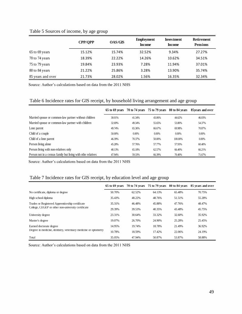
49

Table 5 Sources of income, by age group

Source: Author’s calculations based on data from the 2011 NHS

Table 6 Incidence rates for GIS receipt, by household living arrangement and age group

Source: Author’s calculations based on data from the 2011 NHS

Table 7 Incidence rates for GIS receipt, by education level and age group

Source: Author’s calculations based on data from the 2011 NHS

65 to 69 years 15.12% 15.74% 32.52% 9.34% 27.27%

70 to 74 years 18.39% 22.22% 14.26% 10.62% 34.51%

75 to 79 years 19.84% 23.93% 7.28% 11.94% 37.01%

80 to 84 years 21.22% 25.86% 3.28% 13.90% 35.74%

85 years and over 21.73% 28.02% 1.56% 16.35% 32.34%

Employment

Income

Investment

Income

Retirement

PensionsCPP/QPP OAS/GIS

65 to 69 years 70 to 74 years 75 to 79 years 80 to 84 years 85years and over

Married spouse or common-law partner without children 30.01% 41.34% 43.06% 44.62% 46.03%

Married spouse or common-law partner with children 32.69% 49.34% 55.65% 53.80% 54.37%

Lone parent 49.74% 65.36% 66.67% 69.98% 70.87%

Child of a couple 50.00% 0.00% 0.00% 0.00% 0.00%

Child of a lone parent 46.39% 70.37% 50.00% 100.00% 0.00%

Person living alone 45.28% 57.76% 57.77% 57.93% 60.40%

Person living with non-relatives only 48.13% 65.18% 62.57% 66.40% 66.21%

Person not in a census family but living with othe relatives 47.94% 59.33% 66.39% 70.40% 71.67%

65 to 69 years 70 to 74 years 75 to 79 years 80 to 84 years 85 years and over

No certificate, diploma or degree 50.70% 62.52% 64.13% 65.48% 70.75%

High school diploma 35.43% 48.22% 48.76% 51.51% 55.28%

Trades or Registered Apprenticeship certificate 35.31% 46.48% 45.88% 47.76% 48.47%

College, CEGEP or other non-university certificate29.39% 39.53% 40.35% 43.48% 45.75%

University degree 23.31% 30.64% 33.32% 32.60% 35.92%

Master's degree 19.07% 26.70% 24.90% 25.28% 25.45%

Earned doctorate degree 14.95% 19.74% 18.78% 21.49% 36.92%

Degree in medicine, dentistry, veterinary medicine or optometry10.78% 18.59% 17.42% 22.06% 24.19%

Total 35.05% 47.94% 50.87% 53.87% 58.88%

50

Table 8 Mills lambda, rho, Wald test and number of observations, by age group

*The values in parentheses are p-values.

* % of uncensored observation are slightly different than is the case for Table 7 due to missing data when estimating

the Heckman two-step model. See footnote number 19 for detail.

Source: Author’s calculations based on data from the 2011 NHS

65 to 69 years 70 to 74 years 75 to 79 years 80 to 84 years 85years and over

Mills Lambda -1514.17 -1809.90 -2513.68 -3228.67 -3402.17

(0.00) (0.00) (0.00) (0.00) (0.00)

Rho -0.5572 -0.6723 -0.8325 -0.9503 -0.9919

Wald chi2 1116.32 1279.99 830.18 480.21 291.19

(0.00) (0.00) (0.00) (0.00) (0.00)

N. 39112 28777 22511 15649 10948

Censored observation 25382 14964 11052 7211 4502

Uncensored observation 13730 13813 11459 8438 6446

% of uncensored observation 35.10% 48.00% 50.90% 53.92% 58.88%

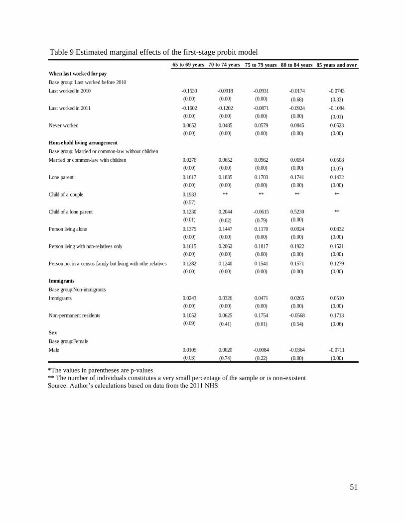
51

Table 9 Estimated marginal effects of the first-stage probit model

*The values in parentheses are p-values

** The number of individuals constitutes a very small percentage of the sample or is non-existent

Source: Author’s calculations based on data from the 2011 NHS

65 to 69 years 70 to 74 years 75 to 79 years 80 to 84 years 85 years and over

When last worked for pay

Base group: Last worked before 2010

Last worked in 2010 -0.1530 -0.0918 -0.0931 -0.0174 -0.0743

(0.00) (0.00) (0.00) (0.68) (0.33)

Last worked in 2011 -0.1602 -0.1202 -0.0871 -0.0924 -0.1084

(0.00) (0.00) (0.00) (0.00) (0.01)

Never worked 0.0652 0.0485 0.0579 0.0845 0.0523

(0.00) (0.00) (0.00) (0.00) (0.00)

Household living arrangement

Base group: Married or common-law without children

Married or common-law with children 0.0276 0.0652 0.0962 0.0654 0.0508

(0.00) (0.00) (0.00) (0.00) (0.07)

Lone parent 0.1617 0.1835 0.1703 0.1741 0.1432

(0.00) (0.00) (0.00) (0.00) (0.00)

Child of a couple 0.1933 ** ** ** **

(0.57)

Child of a lone parent 0.1230 0.2044 -0.0615 0.5230 **

(0.01) (0.02) (0.79) (0.00)

Person living alone 0.1375 0.1447 0.1170 0.0924 0.0832

(0.00) (0.00) (0.00) (0.00) (0.00)

Person living with non-relatives only 0.1615 0.2062 0.1817 0.1922 0.1521

(0.00) (0.00) (0.00) (0.00) (0.00)

Person not in a census family but living with othe relatives 0.1282 0.1240 0.1541 0.1571 0.1279

(0.00) (0.00) (0.00) (0.00) (0.00)

Immigrants

Base group:Non-immigrants

Immigrants 0.0243 0.0326 0.0471 0.0265 0.0510

(0.00) (0.00) (0.00) (0.00) (0.00)

Non-permanent residents 0.1052 0.0625 0.1754 -0.0568 0.1713

(0.09) (0.41) (0.01) (0.54) (0.06)

Sex

Base group:Female

Male 0.0105 0.0020 -0.0084 -0.0364 -0.0711

(0.03) (0.74) (0.22) (0.00) (0.00)

52

Table 9 Estimated marginal effects of the first-stage probit model (continued)

*The values in parentheses are p-values

Source: Author’s calculations based on data from the 2011 NHS

65 to 69 years 70 to 74 years 75 to 79 years 80 to 84 years 85 years and over

Education

Base group: No certificate, diploma or degree

High school diploma -0.1172 -0.1151 -0.1133 -0.1025 -0.1166

(0.00) (0.00) (0.00) (0.00) (0.00)

Trades or Registered Apprenticeship certificate -0.1120 -0.1192 -0.1241 -0.1015 -0.1324

(0.00) (0.00) (0.00) (0.00) (0.00)

College, CEGEP or other non-university certificate -0.1598 -0.1831 -0.1750 -0.1579 -0.1895

(0.00) (0.00) (0.00) (0.00) (0.00)

University -0.2193 -0.2696 -0.2436 -0.2597 -0.2622

(0.00) (0.00) (0.00) (0.00) (0.00)

-0.3187 -0.3422 -0.3980 -0.3193 -0.3322

(0.00) (0.00) (0.00) (0.00) (0.00)

Master's degree -0.2486 -0.2951 -0.3172 -0.3231 -0.3647

(0.00) (0.00) (0.00) (0.00) (0.00)

Earned doctorate degree -0.2816 -0.3632 -0.3731 -0.3385 -0.2172

(0.00) (0.00) (0.00) (0.00) (0.00)

Province or territory of residence in 2010

Base group: Newfoundland and Labrador

Prince Edward Island -0.0479 -0.0841 -0.0855 -0.0836 -0.0580

(0.30) (0.08) (0.09) (0.24) (0.43)

Nova Scotia -0.0390 -0.0879 -0.1295 -0.1518 -0.1184

(0.09) (0.00) (0.00) (0.00) (0.00)

New Brunswick -0.0154 -0.0788 -0.1131 -0.1450 -0.1132

(0.53) (0.00) (0.00) (0.00) (0.01)

Quebec -0.0673 -0.1156 -0.2132 -0.2222 -0.2050

(0.00) (0.00) (0.00) (0.00) (0.00)

Ontario -0.1259 -0.1954 -0.2765 -0.2726 -0.2593

(0.00) (0.00) (0.00) (0.00) (0.00)

Manitoba -0.1126 -0.1725 -0.2286 -0.1848 -0.1771

(0.00) (0.00) (0.00) (0.00) (0.00)

Saskatchewan -0.0703 -0.1163 -0.1888 -0.2043 -0.1505

(0.00) (0.00) (0.00) (0.00) (0.00)

Alberta -0.1215 -0.2080 -0.2507 -0.2235 -0.2121

(0.00) (0.00) (0.00) (0.00) (0.00)

British Columbia -0.0854 -0.1501 -0.2287 -0.2301 -0.2222

(0.00) (0.00) (0.00) (0.00) (0.00)

Northern Canada -0.0063 -0.3955 0.0733 -0.1627 0.1927

(0.92) (0.00) (0.56) (0.55) (0.00)

Official Language

Base group: English only

French only 0.0234 0.0689 0.1354 0.1278 0.1449

(0.04) (0.00) (0.00) (0.00) (0.00)

Both English and French -0.0193 -0.0011 0.0205 0.0334 0.0331

(0.03) (0.92) (0.10) (0.03) (0.06)

Neither English and French -0.0135 0.0223 0.0957 0.1180 0.1450

(0.32) (0.13) (0.00) (0.00) (0.00)

0.3515 0.4805 0.5094 0.5395 0.5891

(0.00) (0.00) (0.00) (0.00) (0.00)

Sample size 39112 28777 22511 15649 10948

Degree in medicine, dentistry, veterinary medicine or optometry

Average predicted probability

53

Table 10 Estimated marginal effects of the corrected outcome equation and the coefficients in the

OLS equation

*The values in parentheses are p-values

* Margin 1: the discrete change from the base level after running Heckman’s sample selection correction procedure.

* Margin 2: average predicted amount of GIS benefit is included

** The number of individuals constitutes a very small percentage of the sample or is non-existent

Source: Author’s calculations based on data from the 2011 NHS

Margin 1 Margin 2 OLS Margin 1 Margin 2 OLS Margin 1 Margin 2 OLS

When last worked for pay

Base group: Last worked before 2010

Last worked in 2010 -260.43 4329.77 -705.43 -206.30 4379.95 -531.14 22.93 5190.2 -439.81

(0.01) (0.00) (0.05) (0.00) (0.90) (0.00)

Last worked in 2011 -233.18 4357.02 -704.36 -112.77 4473.48 -587.30 96.85 5264.12 -421.45

(0.01) (0.00) (0.10) (0.00) (0.31) (0.00)

Never worked 505.36 5095.56 633.38 469.54 5055.79 602.26 483.37 5650.64 793.77

(0.00) (0.00) (0.00) (0.00) (0.00) (0.00)

Household living arrangement

Base group: Married or common-law without children

Married or common-law with children 373.92 4964.12 250.71 263.70 4849.95 426.12 -10.92 5156.35 440.23

(0.00) (0.00) (0.00) (0.00) (0.90) (0.00)

Lone parent 1342.48 5932.68 1363.94 1395.97 5982.22 1791.01 1108.59 6275.86 1692.34

(0.00) (0.00) (0.00) (0.00) (0.00)

Child of a couple 1512.55 6102.75 1846.71 ** ** ** ** ** **

(0.51) (0.19)

Child of a lone parent 1207.95 5798.15 1058.63 885.34 5471.59 1542.55 4311.25 9478.52 2157.34

(0.00) (0.00) (0.07) (0.00) (0.02) (0.05)

Person living alone 1329.80 5920.00 1204.12 1191.56 5777.81 1397.00 984.40 6151.67 1213.44

(0.00) (0.00) (0.00) (0.00) (0.00) (0.00)

Person living with non-relatives only 1553.00 6143.20 1445.41 1366.84 5953.09 1881.35 1342.95 6510.22 1848.54

(0.00) (0.00) (0.00) (0.00) (0.00) (0.00)

Person not in a census family but living with othe relatives 1768.45 6358.65 1412.89 1883.17 6469.42 1750.42 1332.32 6499.59 1793.34

(0.00) (0.00) (0.00) (0.00) (0.00) (0.00)

Immigrants

Base group:Non-immigrants

Immigrants 532.11 5122.31 197.95 506.13 5092.38 245.19 459.71 5626.98 283.83

(0.00) (0.00) (0.00) (0.00) (0.00) (0.00)

Non-permanent residents 1112.39 5702.59 1252.57 757.84 5344.09 852.72 543.96 5711.23 1231.03

(0.01) (0.00) (0.10) (0.01) (0.24) (0.00)

Sex

Base group:Female

Male 291.94 4882.14 165.82 101.62 4687.87 61.33 -28.17 5139.1 -94.40

(0.00) (0.00) (0.00) (0.02) (0.52) (0.00)

Education

Base group: No certificate, diploma or degree

High school diploma -166.19 4424.01 -643.49 -137.49 4448.76 -674.48 75.89 5243.16 -682.22

(0.01) (0.00) (0.01) (0.00) (0.23) (0.00)

Trades or Registered Apprenticeship certificate -211.01 4379.19 -628.84 -247.84 4338.41 -747.62 -187.13 4980.14 -866.35

(0.00) (0.00) (0.00) (0.00) (0.01) (0.00)

College, CEGEP or other non-university certificate -362.53 4227.67 -865.81 -299.46 4286.79 -1059.24 -67.07 5100.2 -1092.24

(0.00) (0.00) (0.00) (0.00) (0.45) (0.00)

University -276.76 4313.44 -1032.84 -106.21 4480.04 -1251.64 18.34 5185.61 -1261.06

(0.01) (0.00) (0.30) (0.00) (0.86) (0.00)

Degree in medicine, dentistry, veterinary medicine or

optometry

922.11 5512.31 -932.20 610.69 5196.94 -1019.54 1984.87 7152.14 -1205.69

(0.07) (0.00) (0.13) (0.00) (0.00) (0.00)

Master's degree -412.22 4177.98 -1121.0 -62.39 4523.86 -1327.74 635.80 5803.07 -1295.36

(0.01) (0.00) (0.69) (0.00) (0.00) (0.00)

Earned doctorate degree 325.14 4915.34 -1054.74 545.13 5131.38 -1322.66 1086.73 6254 -1311.12

(0.26) (0.00) (0.07) (0.00) (0.00) (0.00)

Average predicted amount of GIS benefits

Uncensored observation

65 to 69 years 70 to 74 years 75 to 79 years

4590.2 4586.25 5167.27

13730 13813 11459

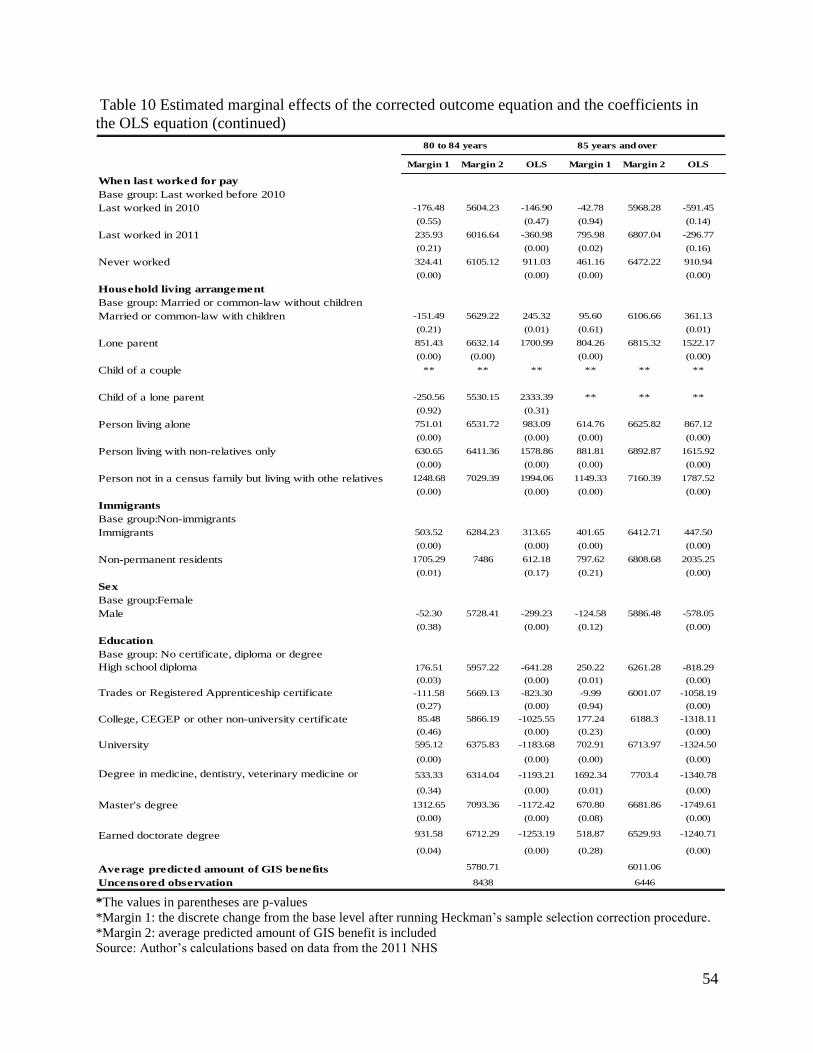
54

Table 10 Estimated marginal effects of the corrected outcome equation and the coefficients in

the OLS equation (continued)

*The values in parentheses are p-values

*Margin 1: the discrete change from the base level after running Heckman’s sample selection correction procedure.

*Margin 2: average predicted amount of GIS benefit is included

Source: Author’s calculations based on data from the 2011 NHS

Margin 1 Margin 2 OLS Margin 1 Margin 2 OLS

When last worked for pay

Base group: Last worked before 2010

Last worked in 2010 -176.48 5604.23 -146.90 -42.78 5968.28 -591.45

(0.55) (0.47) (0.94) (0.14)

Last worked in 2011 235.93 6016.64 -360.98 795.98 6807.04 -296.77

(0.21) (0.00) (0.02) (0.16)

Never worked 324.41 6105.12 911.03 461.16 6472.22 910.94

(0.00) (0.00) (0.00) (0.00)

Household living arrangement

Base group: Married or common-law without children

Married or common-law with children -151.49 5629.22 245.32 95.60 6106.66 361.13

(0.21) (0.01) (0.61) (0.01)

Lone parent 851.43 6632.14 1700.99 804.26 6815.32 1522.17

(0.00) (0.00) (0.00) (0.00)

Child of a couple ** ** ** ** ** **

Child of a lone parent -250.56 5530.15 2333.39 ** ** **

(0.92) (0.31)

Person living alone 751.01 6531.72 983.09 614.76 6625.82 867.12

(0.00) (0.00) (0.00) (0.00)

Person living with non-relatives only 630.65 6411.36 1578.86 881.81 6892.87 1615.92

(0.00) (0.00) (0.00) (0.00)

Person not in a census family but living with othe relatives 1248.68 7029.39 1994.06 1149.33 7160.39 1787.52

(0.00) (0.00) (0.00) (0.00)

Immigrants

Base group:Non-immigrants

Immigrants 503.52 6284.23 313.65 401.65 6412.71 447.50

(0.00) (0.00) (0.00) (0.00)

Non-permanent residents 1705.29 7486 612.18 797.62 6808.68 2035.25

(0.01) (0.17) (0.21) (0.00)

Sex

Base group:Female

Male -52.30 5728.41 -299.23 -124.58 5886.48 -578.05

(0.38) (0.00) (0.12) (0.00)

Education

Base group: No certificate, diploma or degree

High school diploma 176.51 5957.22 -641.28 250.22 6261.28 -818.29

(0.03) (0.00) (0.01) (0.00)

Trades or Registered Apprenticeship certificate -111.58 5669.13 -823.30 -9.99 6001.07 -1058.19

(0.27) (0.00) (0.94) (0.00)

College, CEGEP or other non-university certificate 85.48 5866.19 -1025.55 177.24 6188.3 -1318.11

(0.46) (0.00) (0.23) (0.00)

University 595.12 6375.83 -1183.68 702.91 6713.97 -1324.50

(0.00) (0.00) (0.00) (0.00)

Degree in medicine, dentistry, veterinary medicine or

optometry

533.33 6314.04 -1193.21 1692.34 7703.4 -1340.78

(0.34) (0.00) (0.01) (0.00)

Master's degree 1312.65 7093.36 -1172.42 670.80 6681.86 -1749.61

(0.00) (0.00) (0.08) (0.00)

Earned doctorate degree 931.58 6712.29 -1253.19 518.87 6529.93 -1240.71

(0.04) (0.00) (0.28) (0.00)

Average predicted amount of GIS benefits

Uncensored observation

80 to 84 years 85 years and over

5780.71 6011.06

8438 6446

55

Figure 1 Low income rates among seniors 1976 to 2009

Source: The Figure was completed using data from Description for Figure 3.2 of Murphy et al. (2012).

Figure 2 Number of persons in low income status by age and sex (x 1,000), 1976-2009

Source: Author’s calculations based on data from CANSIM Table 206-0041 Low income statistics

Figure 3 Average income of seniors and non-seniors, 1976-2009

Source: The Figure was completed using data from Description for Figure 3.2 of Murphy et al. (2012).

0

5

10

15

20

25

30

35

19

76

19

77

19

78

19

79

19

80

19

81

19

82

19

83

19

84

19

85

19

86

19

87

19

88

19

89

19

90

19

91

19

92

19

93

19

94

19

95

19

96

19

97

19

98

19

99

20

00

20

01

20

02

20

03

20

04

20

05

20

06

20

07

20

08

20

09

LICO LIM MBM

0

100

200

300

400

500

600

700

800

19

76

19

77

19

78

19

79

19

80

19

81

19

82

19

83

19

84

19

85

19

86

19

87

19

88

19

89

19

90

19

91

19

92

19

93

19

94

19

95

19

96

19

97

19

98

19

99

20

00

20

01

20

02

20

03

20

04

20

05

20

06

20

07

20

08

20

09

20

10

20

11

20

12

20

13

20

14

Persons 65 years and over Males, 65 years and over Females, 65 years and over

0

5000

10000

15000

20000

25000

30000

19

76

19

77

19

78

19

79

19

80

19

81

19

82

19

83

19

84

19

85

19

86

19

87

19

88

19

89

19

90

19

91

19

92

19

93

19

94

19

95

19

96

19

97

19

98

19

99

20

00

20

01

20

02

20

03

20

04

20

05

20

06

20

07

20

08

20

09

Non-seniors Seniors