Investig

atin

g N

on

-Price F

acto

rs in E

lectricity Dem

an

d R

espo

nse:

Supervisors: Prof. dr. Steven Van Passel and Dr. Erik Laes

Doctoral dissertation submitted to obtain the degree of

Doctor in Applied Economics

Faculty of Business and Economics - Antwerp, 2019

Investigating Non-Price Factors

in Electricity Demand Response:

An Applied Economics Study

Aman Srivastava

FACULTY OF BUSINESS AND ECONOMICS

DISSERTATION

Investigating Non-Price Factors in Electricity Demand Response: An

Applied Economics Study

THESIS SUBMITTED IN ORDER TO OBTAIN THE DEGREE OF

DOCTOR IN APPLIED ECONOMICS

Aman SRIVASTAVA

Supervisors Prof. dr. Steven VAN PASSEL Dr. Erik LAES

Antwerp

September 2019

Supervisors Prof. dr. Steven VAN PASSEL (University of Antwerp) Dr. Erik LAES (VITO and TU Eindhoven)

Members of the Examination Committee Prof. dr. Herbert PEREMANS (University of Antwerp) Prof. dr. Erik DELARUE (KU Leuven) Dr. Pieter VALKERING (VITO) Prof. dr. Ivan VERHAERT (University of Antwerp) Prof. dr. Geert VERBONG (TU Eindhoven) Prof. dr. David SHIPWORTH (University College London)

ISBN: 978-90-8994-200-5 Cover image: Akash Kumar and Viraj Kumar Cover design: University of Antwerp Printing and binding: Universitas, Antwerp © Copyright 2019, Aman SRIVASTAVA All rights reserved. No part of this publication maybe reproduced or transmitted in any form or by any means, electronic or mechanical, including photocopying, recording, or by any information storage and retrieval system, without permission in writing from the author.

How long will we remain content celebrating our potential Even as we restrain ourselves from realizing it?

Anonymous

There rolls the deep where grew the tree. O earth, what changes hast thou seen!

Alfred, Lord Tennyson

i

Publications This thesis is based on the following publications and working papers:

Srivastava, A., Van Passel, S., Valkering, P., & Laes, E. Gridding India of power cuts: A choice experiment to introduce residential demand response in a developing country. Working paper

Srivastava, A., Van Passel, S., Kessels, R., Valkering, P., & Laes, E. Reducing winter peaks in electricity consumption: A choice experiment to structure demand response programs. Working paper

Srivastava, A., Van Passel, S., & Laes, E. (2019). Dissecting demand response: A quantile analysis of flexibility, household attitudes, and demographics. Energy Research and Social Science, 52, 169-180. Available at https://doi.org/10.1016/j.erss.2019.02.011

Srivastava, A., Van Passel, S., & Laes, E. (2018). Assessing the success of electricity demand response programs: A meta-analysis. Energy Research and Social Science, 40, 110-117. Available at https://doi.org/10.1016/j.erss.2017.12.005

ii

iii

Acknowledgements I had already been working in research for several years, and a doctorate was a logical next step to build my career. After searching through programs and professors’ profiles in several universities across numerous countries, through a chain of events I ended up pursuing it in Belgium. With my prior research experience, and having lived in four countries already – five, if you count Scotland separately – I thought to myself, how hard could it be? If I could, I’d knock 2016 me on the head for that cockiness. Looking back, I wasn’t prepared for all the changes that followed. Living in Antwerp was challenging. Particularly for someone who’d never visited Belgium before, who didn’t speak the local language, who didn’t know a single person there, and who consequently couldn’t immediately grasp the local culture. The doctorate was challenging: meta-analyses, R, quantile regressions, impact factors, H-indices – this was all Flemish to me. Also, so many existential questions! Was I a student or an employee? Where in the world was Genk? WHY was everyone eating sandwiches all the time? There were so many things that I had to get used to. It might have been easy to get overwhelmed. Maybe I did, a little, and that’s why I scurried off to live in Brussels. But over time, the transition to a new life was made easier thanks to the company of new friends, the reunions with old friends, and the sustained support of my extended family. And while I am grateful to many who supported my spirits through this journey, from first stumbles to final sprint, I would be remiss if I didn’t specifically acknowledge some of the key people here. First, the biggest thanks go to Steven, for his trust and guidance, for giving me the independence and flexibility to work my way, and for pushing me – encouragingly – when I asked him to. In similar vein, Erik and Pieter have been my extremely supportive guides at VITO, and I want to thank them for all their feedback and encouragement. For the administrative support, I’m also grateful to An, Esmeralda, Lesley, Vera, and Joeri. To the old friends and family who visited or traveled with me – Joe, Denise, 3PM, Francis, Emily, Molly, Tianyi, Maximus, Pritamma, Venkat mausa, Taniage & Serban, Phil, Murli, Bah-su, EJ – your visits were like packets of warm rice in a field of cold bread. And to the friends from an earlier life who happened to be living around Brussels – Anna, Maïte, Stan – you provided a welcome touch of familiarity, and I hope our paths keep crossing. On to the newer, then; to my daily enablers and the main focus of this section. Alanito & Cynthia, Amalie, and Flo (together the Guardians) were among my first friends here. I was in a strange land, hobbled by a torn ligament and a grumpy personality. These guys welcomed me and helped me survive the first year, with all their help in moving, the board games and cocktails, the meals at Giovanni’s and Amadeus, the sandwichon and Game of Thrones, beers at ’t Waagstuk, and more. WC Paul and Loïc joined during my second year and – with Karsten – soon also became my good friends. Paul brought along intellectual stimulation, contrarian views, and a socio-political like-mindedness. Loic, whose moral corruption I engineered, was a great office-mate and all-round

iv

helpful person, and whatever his future achievements may be, I just hope he watches It’s Always Sunny. In Karsten, I found someone who shared my musical tastes, travel styles, and love of frugality. Starting in my second year, board games were replaced by beers, pushing boundaries became a bit of a norm, and my social life started gravitating back to Antwerp, even though I was always running to catch the train back to Brussels. Gabi & Vasco were also great new company starting around this time, whenever I had the chance to see them, and Carlos was always willing to bring good cheer and a listening ear. Although I spent a fair amount of time in India in my third year, I also enjoyed hanging out with Patrick (with whom my pee breaks were curiously synchronized), Michele, and Wito at the university. With this community, together with the fifth floor gang, university lunches became larger affairs. The days started to include more coffee breaks, afternoon walks around the courtyard, and office sitcom screenings. Kassa 4 became more deeply entrenched as a firm favorite. And this year – with spas, ghost towns, Jordan, swimming & Turkish pizzas – created some exceptional memories. Erin brought along some good old DC nostalgia with her, and I spent many other hours talking about DC, politics, policy, and inane matters with Emily and Carlo. With these three, I explored Brussels, complained about Belgian bureaucracy, and discovered good salsa. Artus, with Patrice, helped make life at 137AHJ just a bit funnier. Overpriced art, evening whiskies, Heineken merchandise, de-icing swords, miners’ lamps, and missing bonsais; life there was certainly ridiculous, yet homely. And I can’t not acknowledge my awesome guitar teachers, first Marianna and then Nikos, whose dedication to their art helped take my mind off of research and made me aspire to other things. And now, in my fourth year, though there are no more new people, I do have more new memories: of intense trips, jerk pigeons, crazy festivals, and more. And that’s it. This has been a difficult, rewarding, learning, humbling, and enriching experience, and I think I am so much the better for it. But 2019 is a year of change. So, a little earlier than I could have hoped for, and a little more sadly than I’d expected, it is time to close this chapter. It is also time to open a new one, and I have a feeling it’s going to be a real page-turner for young Dr. Srivastava. And in closing, to my family: Thank you for always being the home that I could return to. Onwards and upwards…

Aman SRIVASTAVA Antwerp, September 2019

v

Summary in English Globally, the electricity sector is responsible for a large share of greenhouse gas emissions, and is also in need of new infrastructure investments. An ongoing and accelerating transition to the generation of electricity from renewable energy sources can help mitigate the former, but the variabilities in supply can create further challenges in the security of energy supply. Demand response programs aim to induce flexibility in the patterns of electricity demand – through for instance the time-based pricing of electricity or through external controls on its usage at certain times of the day – such that this demand may be better aligned with the supply. In doing so, they can support the energy transition and help to address the energy security concerns. Further, in developing countries, their strategic implementation could potentially contribute to improving energy access and grid stability, while helping to leapfrog investments in traditional infrastructure. Such demand response programs have been successfully implemented in the industrial and commercial sectors of many countries. Their trials and rollouts in the residential sectors have however had mixed success, despite a large potential for flexibility. Existing literature suggests that this is because with households, there are a greater number of behavioral considerations that should be taken into account, and a number of non-price factors can also influence behavior in addition to pricing incentives. Studies have independently identified roles for enhanced information, supporting technologies, respondent demographics, and customer biases and / or preferences in shaping response. However, two gaps stand out in this range of literature. The first is that many of these non-price factors have been studied in isolation, independently of each other, and only in single-case contexts. The second gap is that most research and implementation has taken place in industrialized countries, even though the potential benefits of demand response are arguably even higher in the developing world. This thesis contributes towards addressing these two gaps through a multi-tool analysis of demand response in several countries. As a first step, it improves upon findings from existing experiences with demand response using a mix of two approaches. In the first of these, it collects several demand response programs from across countries and systematically analyzes them to determine how their success and failure was linked to shared characteristics in their design and in the local socio-economic environments – this offers global lessons on the types of enabling environments that should be in place to improve the likelihood of a successful implementation. Secondly, it slices into a single demand response program to determine how the varying levels of customer responsiveness relate to participants’ differences in attitudes and concerns. This indicates that even within a single demand response program, different communication and incentive strategies will be required among different segments of customers in order to first induce and then increase response. In a second step, the thesis then applies these lessons towards identifying designs for demand response that are likely to have broad customer acceptance. It does so in one developed country –

vi

Belgium – and one developing country – India – to illustrate how the design and implementation requirements converge based on commonalities in enabling environments, and how they must vary in line with the local contexts and population characteristics. Through this, it also demonstrates that when respondents even within a single country are grouped into clusters based on their preferences, these differing preferences are correlated with different sets of shared characteristics, again highlighting that there’s a need for a range of approaches to induce flexibility among all the population groups. In this way, the second step of the thesis also corroborates and advances the lessons from the concluded studies while offering actionable solutions. By using analytical methods that haven’t previously been used in this field, applying lessons from existing experiences to design future initiatives, and studying the implications in two countries that are at different stages in their development, the thesis offers globally and locally relevant lessons for policymakers and researchers around the world.

vii

Summary in Dutch De elektriciteitssector is wereldwijd verantwoordelijk voor een groot deel van de schadelijke uitstoot van broeikasgassen en investeringen in nieuwe infrastructuur voor de opwekking en het transport van elektriciteit zijn nodig. Een voortdurende en versnelde overgang naar de opwekking van elektriciteit uit hernieuwbare energiebronnen kan bijdragen tot een vermindering van de uitstoot van broeikasgassen. De fluctuaties in energievoorziening kunnen nieuwe uitdagingen met zich meebrengen voor de continuïteit van energievoorziening.

Programma's om in te spelen op de vraag naar elektriciteit, zogenaamde vraagrespons-programma’s zijn erop gericht om de vraag naar elektriciteit aanpasbaar te maken. Dit gebeurt bijvoorbeeld door middel van een op tijd gebaseerde prijsstelling voor elektriciteit of door externe controles op het gebruik ervan op bepaalde tijdstippen van de dag. De vraag wordt zo beter afgestemd op het aanbod. Op die manier kunnen de vraagrespons-programma’s de energietransitie ondersteunen en bijdragen tot het verminderen van de energieonzekerheid. Voorts kan de strategische uitvoering van deze maatregelen in ontwikkelingslanden mogelijk bijdragen tot een betere toegang tot energie en een stabieler netwerk. Tegelijkertijd helpen de investeringen om een sprong voorwaarts te maken en de infrastructuur te moderniseren.

Dergelijke vraagrespons-programma's zijn met succes geïmplementeerd in zowel de industriële- als de commerciële sectoren van veel landen. De testfase en implementatie in de residentiële sector kent echter een wisselend succes, ondanks het grote potentieel van een flexibele vraag. De bestaande literatuur suggereert dat dit bij huishoudens te maken heeft met het groot aantal gedragsoverwegingen, alsook een aantal andere factoren die niet prijs gedreven zijn. Studies hebben onafhankelijk van elkaar de rol van verbeterde informatie, ondersteunende technologieën, de demografie van de respondent, en de voorkeur van de klant geïdentificeerd als belangrijke factoren bij het succes van dergelijke vraagrespons-programma’s.

Er zijn echter twee lacunes in de literatuur. De eerste is dat veel van deze niet-prijsfactoren geïsoleerd, onafhankelijk van elkaar, en slechts in een enkele case studie zijn onderzocht. De tweede lacune is dat het grootste deel van het onderzoek en de implementatie heeft plaatsgevonden in de geïndustrialiseerde landen, ook al zijn de potentiële voordelen van vraagrespons in de ontwikkelingslanden aantoonbaar groter.

Dit proefschrift draagt bij tot de literatuur door zich te richten op deze lacunes en gebruik te maken van een multi-tool analyse van de vraagrespons in verschillende landen. Vooreerst verbetert het de bestaande resultaten door de vraag op twee manieren te benaderen. In de eerste benadering worden verschillende vraagrespons-programma's uit verschillende landen verzameld en gezamenlijk geanalyseerd. Hieruit wordt vastgesteld hoe hun succes en falen in verband werd gebracht met gemeenschappelijke kenmerken zoals het ontwerp van het programma en de socio-economische situatie. Deze vaststellingen bieden wereldwijde lessen over welke faciliterende omgevingen gecreëerd moeten worden opdat de kans op een succesvolle implementatie kan worden verhoogd. De tweede benadering onderzoekt een specifiek vraagrespons-programma om te bepalen hoe de verschillende reacties van potentiële klanten zich verhouden tot de verschillen in houding en bezorgdheden van deze deelnemers. De resultaten geven aan dat zelfs binnen één vraagrespons-programma verschillende communicatie- en prikkels nodig zullen zijn. De verschillende

viii

strategieën moeten zich richten op de verschillende segmenten van klanten, om zo een flexibele vraag te bewerkstelligen en vervolgens te vergroten.

Vervolgens past dit proefschrift in een tweede deel de inzichten toe op het identificeren van succesvolle ontwerpen van vraagrespons-programma’s. Dit deel bekijkt één ontwikkeld land – België – en één ontwikkelingsland – Indië – om te illustreren hoe de ontwerp- en implementatievereisten convergeren op basis van gemeenschappelijke kenmerken en hoe ze moeten variëren in functie van de lokale context en bevolkingskenmerken. Het toont ook aan dat wanneer respondenten, zelfs binnen één land, worden gegroepeerd in clusters op basis van hun voorkeuren, deze verschillende voorkeuren gecorreleerd zijn met diverse reeksen van gemeenschappelijke kenmerken. Dit benadrukt nogmaals dat er behoefte is aan verschillende benaderingen om flexibiliteit te bewerkstelligen. Op deze manier bevestigt het tweede deel van dit proefschrift het eerste deel, terwijl tegelijkertijd bruikbare oplossingen worden geboden.

Door gebruik te maken van analytische methoden die niet eerder in deze context aangewend werden, inzichten toe te passen op het ontwerp van toekomstige initiatieven, en het onderzoeken van de implementatie in twee verschillende landen, biedt dit proefschrift op globaal en lokaal niveau relevante lessen voor beleidsmakers en onderzoekers.

ix

Contents

Publications ....................................................................................................................................... i Acknowledgements ......................................................................................................................... iii Summary in English ......................................................................................................................... v

Summary in Dutch ......................................................................................................................... vii

1. INTRODUCTION .............................................................................................................................. 1 1.1 Demand Response .................................................................................................................. 1

1.1.1 Definitions ..................................................................................................................... 1

1.1.2 Demand Response in Developed Countries .................................................................. 3 1.1.3 Demand Response in Developing Countries ................................................................. 4

1.2 Research Background and Key Questions ............................................................................. 5 1.2.1 Theoretical Background and Gaps ................................................................................ 5 1.2.2 Research Objective ........................................................................................................ 6

1.3 Thesis Approach and Outline ................................................................................................. 7 1.3.1 Chapter 2: A Meta-Analysis of Common Features ....................................................... 8 1.3.2 Chapter 3: A Quantile Analysis of Constituent Factors ................................................ 9 1.3.3 Chapter 4: Load Controls in a Developed Country ....................................................... 9 1.3.4 Chapter 5: Dynamic Pricing in a Developing Country ................................................. 9

1.4 Discussion on Methods ........................................................................................................ 10 1.4.1 Meta-Analyses ............................................................................................................. 11 1.4.2 Quantile Regressions ................................................................................................... 14 1.4.3 Discrete Choice Experiments ...................................................................................... 15

1.5 The Economics of Demand Response Programs ................................................................. 17 1.6 Emerging Complementary Demand-Side-Management Initiatives ..................................... 19

1.6.1 Increasing Penetration of Renewables and Rooftop Solar Photovoltaics ................... 19

1.6.2 Behind-the-Meter Storage ........................................................................................... 20 1.6.3 Electric Vehicles and Vehicle-to-Grid Charging ........................................................ 21

1.6.4 Heat Pumps ................................................................................................................. 21 1.6.5 Energy Aggregators..................................................................................................... 22 1.6.6 Peer-to-Peer Energy Sharing and Virtual Power Plants .............................................. 22

1.7 A Note on Energy and Electricity ........................................................................................ 23 1.8 Research Framework and Closing Thoughts ....................................................................... 23 References .................................................................................................................................. 25

x

2. A META-ANALYSIS OF COMMON FEATURES ............................................................................... 39 2.1 Introduction .......................................................................................................................... 39

2.2 Methods ................................................................................................................................ 41

2.2.1 Data Gathering and Categorization ............................................................................. 41 2.2.2 Boundaries of Meta-Analyses ..................................................................................... 45 2.2.3 Regression Equation .................................................................................................... 45

2.3 Results .................................................................................................................................. 46 2.3.1 Identifying a Base Model ............................................................................................ 46

2.3.2 Robustness against Alternatives .................................................................................. 48 2.3.3 Caution in Interpreting the Results .............................................................................. 49

2.4 Discussion ............................................................................................................................ 50 2.5 Conclusion ........................................................................................................................... 51 Appendix 2-A: Demand Response Initiatives and Data on Select Variables ............................ 53 Appendix 2-B: Additional Sensitivity Analyses ........................................................................ 55 References .................................................................................................................................. 57 3. A QUANTILE ANALYSIS OF CONSTITUENT FACTORS .................................................................... 65

3.1 Introduction .......................................................................................................................... 65 3.1.1 Demand Response ....................................................................................................... 65 3.1.2 Literature on Household Response to Demand Response ........................................... 66 3.1.3 Scope of Current Study ............................................................................................... 67

3.2 The Linear Smart Grid Trial ................................................................................................. 68

3.3 Methods ................................................................................................................................ 71 3.3.1 Research Method: Quantile Regression ...................................................................... 71 3.3.2 Research Design: Data and Pre-processing ................................................................. 72

3.4 Results .................................................................................................................................. 73 3.5 Discussion ............................................................................................................................ 81

3.5.1 Age .............................................................................................................................. 81

3.5.2 Perceived Benefits from Using Smart Appliances ...................................................... 82 3.5.3 Usage of Smart Appliances ......................................................................................... 82

3.5.4 The Role of Subsidies in Deciding to Buy Smart Appliances .................................... 82 3.5.5 Behavior Changes over the Course of the Field Test .................................................. 83

3.6 Conclusions and Policy Implications ................................................................................... 83 Appendix 3-A: Predictor Variables ............................................................................................ 86 Appendix 3-B: Diagnostics for Model OLS Regression ............................................................ 88 References .................................................................................................................................. 89

xi

4. ESTIMATING ACCEPTABILITY: LOAD CONTROLS IN A DEVELOPED COUNTRY .............................. 93 4.1 Introduction .......................................................................................................................... 93

4.1.1 Opportunity for Demand Response in Belgium .......................................................... 94

4.1.2 Scope of Paper ............................................................................................................. 95 4.2 Methods ................................................................................................................................ 95

4.2.1 Discrete Choice Experiments ...................................................................................... 95

4.2.2 Background Literature and Consultations ................................................................... 97 4.2.3 Pilot Choice Experiment ............................................................................................. 98

4.2.4 Main Choice Experiment ............................................................................................ 99 4.3 Results ................................................................................................................................ 101

4.3.1 Respondent Characteristics ....................................................................................... 101 4.3.2 Modeling Results....................................................................................................... 102 4.3.3 Policy Simulations..................................................................................................... 104 4.3.4 Economic Value of Demand Response Implementation ........................................... 106

4.4 Conclusion and Policy Implications ................................................................................... 107 Appendix 4-A: Survey Questionnaire ...................................................................................... 109 Appendix 4-B: Pilot Design and Results .................................................................................. 113

References ................................................................................................................................ 115 5. ESTIMATING ACCEPTABILITY: DYNAMIC PRICING IN A DEVELOPING COUNTRY ........................ 121

5.1 Introduction ........................................................................................................................ 121 5.1.1 Demand Response in Developed Countries .............................................................. 121

5.1.2 Demand Response in Developing and Emerging Countries ..................................... 122 5.1.3 Scope of Paper ........................................................................................................... 123

5.2 The Domestic Context ........................................................................................................ 123

5.2.1 Uneven Access to Electricity .................................................................................... 123 5.2.2 Support for Renewable Energy ................................................................................. 124 5.2.3 Inefficient Subsidies .................................................................................................. 124

5.2.4 Electricity Usage Profile in Delhi: A Mismatch with Utility Costs .......................... 124 5.2.5 Retail and Demographic Trends: Increasing Reliance on Appliances ...................... 126

5.2.6 Experience with and Potential for Demand Response .............................................. 126 5.3 Research Method and Design ............................................................................................. 127

5.3.1 Research Method: Discrete Choice Experiment ....................................................... 127 5.3.2 Research Design ........................................................................................................ 129

5.4 Results ................................................................................................................................ 132 5.4.1 Sample Statistics ....................................................................................................... 132

xii

5.4.2 Logit Model Results .................................................................................................. 135 5.5 Discussion and Policy Implications ................................................................................... 137

5.5.1 Discussion of Estimates ............................................................................................ 137

5.5.2 Cluster Analysis of Preferences ................................................................................ 139 5.5.3 General Utility-Based Options .................................................................................. 141 5.5.4 Specific Enrollment-Based Options .......................................................................... 142

5.5.5 Economic Value of Demand Response Implementation ........................................... 144 5.6 Conclusion .......................................................................................................................... 144

Appendix 5-A: Survey Questionnaire ...................................................................................... 147 References ................................................................................................................................ 153

6. OVERALL CONCLUSIONS ........................................................................................................... 163

6.1 Summary of Contributions ................................................................................................. 163 6.2 Chapter Conclusions .......................................................................................................... 164

6.2.1 Concluding Remarks for Chapter 2 ........................................................................... 164 6.2.2 Concluding Remarks for Chapter 3 ........................................................................... 164 6.2.3 Concluding Remarks for Chapter 4 ........................................................................... 165

6.2.4 Concluding Remarks for Chapter 5 ........................................................................... 165 6.3 Overall Conclusions ........................................................................................................... 166

6.3.1 Common Lessons ...................................................................................................... 167 6.3.2 Lessons from the Belgian Context ............................................................................ 168 6.3.3 Lessons from the Indian Context .............................................................................. 170

6.4 Limitations ......................................................................................................................... 172 6.5 Academic Contributions and Future Research ................................................................... 173

6.5.1 Academic Contributions ............................................................................................ 173

6.5.2 Future Research ......................................................................................................... 174 References ................................................................................................................................ 175

1

Introduction 1. 1.1 Demand Response While more research has historically been conducted upon the supply side of electricity – towards increasing production, improving the grid, changing the generation mix – the demand for electricity is an increasing area of focus. Bloomberg New Energy Finance (BNEF) projects that global electricity demand will increase by 57% above current levels by 2050 [1], indicating a need for improved demand side management (DSM) of electricity. Of the various DSM tools available, energy efficiency (EE) measures aim to help reduce demand from individual appliances or buildings, and to thereby reduce the growth in demand overall. Distributed generation and energy storage solutions can reduce the constant dependence on a grid, although their applications are limited since they are expensive and inefficient at present [2,3] – a discussion on these and other emerging DSM avenues is enclosed in Section 1.6. The third main tool in the DSM kit, demand response (DR), can shift the patterns of electricity demand in ways that can have multiple benefits. This DSM instrument is the one upon which this thesis focuses. 1.1.1 Definitions DR programs aim to encourage shifts in the patterns of electricity demand in response to incentives, particularly during peak periods, as a means of balancing supply and demand. They do this mainly via either pricing-based mechanisms – such as time-of-use (ToU) pricing, critical peak pricing (CPP), real time pricing (RTP), and critical peak rebates (CPR) – or via incentive-based mechanisms such as direct load control programs1. ToU pricing usually involves two or three different rates that are offered at different times of the day, such as peak, partial peak, and off-peak – these time blocks and rates are pre-determined. Typically, lower rates are offered during the daytime off-peak hours when aggregate electricity demand is lower, and higher rates are offered during the evening peak hours, to encourage a shift away from peak hours [4]. Unlike ToU pricing, CPP is less regular and more event-based. CPP plans impose very high rates – up to 15 times the standard rates [5,6] – during critical peak events for a few hours on a small number of days per year. For the rest of the time, they maintain standard – or pre-determined ToU – rates. CPR is similar to CPP, except that the customer receives a refund for reducing consumption during the critical peak events [4]. Lastly among the pricing-based mechanisms, RTP programs generally imply pricing that varies on an hourly basis, determined by wholesale market prices and communicated to customers either the day before or in real-time [4,7]. While ToU pricing may be the easiest for customers to track due

1 These can be supplemented by moral norms, i.e. appeals to customers to behave in a manner that is consistent with their values and also beneficial to the electricity system

2

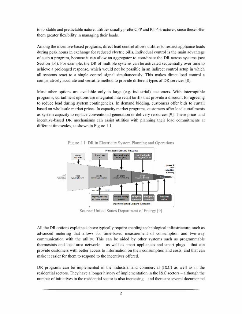
to its stable and predictable nature, utilities usually prefer CPP and RTP structures, since these offer them greater flexibility in managing their loads. Among the incentive-based programs, direct load control allows utilities to restrict appliance loads during peak hours in exchange for reduced electric bills. Individual control is the main advantage of such a program, because it can allow an aggregator to coordinate the DR across systems (see Section 1.6). For example, the DR of multiple systems can be activated sequentially over time to achieve a prolonged response, which would not be possible in an indirect control setup in which all systems react to a single control signal simultaneously. This makes direct load control a comparatively accurate and versatile method to provide different types of DR services [8]. Most other options are available only to large (e.g. industrial) customers. With interruptible programs, curtailment options are integrated into retail tariffs that provide a discount for agreeing to reduce load during system contingencies. In demand bidding, customers offer bids to curtail based on wholesale market prices. In capacity market programs, customers offer load curtailments as system capacity to replace conventional generation or delivery resources [9]. These price- and incentive-based DR mechanisms can assist utilities with planning their load commitments at different timescales, as shown in Figure 1.1.

Figure 1.1: DR in Electricity System Planning and Operations

Source: United States Department of Energy [9]

All the DR options explained above typically require enabling technological infrastructure, such as advanced metering that allows for time-based measurement of consumption and two-way communication with the utility. This can be aided by other systems such as programmable thermostats and local-area networks – as well as smart appliances and smart plugs – that can provide customers with better access to information on their consumption and costs, and that can make it easier for them to respond to the incentives offered. DR programs can be implemented in the industrial and commercial (I&C) as well as in the residential sectors. They have a longer history of implementation in the I&C sectors – although the number of initiatives in the residential sector is also increasing – and there are several documented

3

instances of such initiatives around the world. For example, the building materials supplier Hanson UK has rolled out DR across 29 quarries in Britain, in partnership with an aggregator, to deliver 2 megawatts (MW) of flexibility [10]. In the United Stated (US), San Diego Gas & Electric has a program that uses load controls on heating, ventilation, and air conditioning (HVAC) systems in the commercial sector for up to four hours at a time, in exchange for annual credits on the customers’ bills [11]. Similarly, Pacific Gas & Electric has a range of DR programs available for small and medium businesses, including peak day pricing, automated DR, and base interruptible programs [12]. Even in India, a power utility launched an automated DR project in the capital city of Delhi among select I&C customers with a load in excess of 100 kW and covering a total connected load of 400 MW. The shed potential of this project was estimated at 20 MW [13]. Consequently, an extensive body of literature on the DR experience in the I&C sectors already exists [14,15,16,17,18], and larger gaps remain in research into household DR. This thesis studies the feasibility of DR programs from the perspectives of residential customers, which are less understood – in studying this, it does not consider their benefits from the perspectives of the utility companies, a topic which is briefly discussed in Section 1.5. This scope of research within this thesis is further explained in Sections 1.2 and 1.3. 1.1.2 Demand Response in Developed Countries The electricity sector in developed countries is faced with two medium- to long-term challenges. First, it is a significant contributor to climate change, with for instance nearly 30% of total greenhouse gases (GHG) emitted in the US coming from electricity production [19]. At the same time, the ageing grid infrastructure, combined with the ongoing transition to renewable sources [20] that are more variable in generation, presents a challenge for the security of energy supply. For instance, temporary outages in Belgium’s nuclear power plants led to a decline in generation of nearly 24% between 2010 and 2014, though the amounts have rebounded since then [21]. These challenges exist within the context of projected increases in electricity demand, driven by greater electrification of heating and transport. These projected increases in electricity demand are an important driver of the expected value in demand side flexibility. By introducing flexibility in consumption patterns, DR can also make it easier to integrate the variable generation from renewable sources into the mix. Further, by flattening the peaks in demand, it can reduce the need for generation from peaking power plants, which are typically more expensive and polluting [22,23]. For instance, in Ontario (Canada), 3% of the peak load arises in less than 15 hours during a year, but it costs more than 130 million US dollars annually to maintain the peak generation capacity [24]. The total potential for DR to shift consumption in 40 European countries alone has been estimated at 160 gigawatts (GW) by 2030, with around 40% of this potential coming from the residential sector [25]. The total theoretical DR potential for 34 European countries was separately assessed as being 52 GW (9.4% of cumulative peak load) split into residential (42%), industrial (31%) and commercial (27%) sectors [26], although the achievable potential is likely lower [27]. In the US, as of 2015, DR programs alone were estimated to have the potential of 31 GW, accounting for 6.6% of total peak demand of all system operators, and it was estimated that DR would probably shave

4

38,000 MW off the country’s peak demand in the year 2019 [28]. US estimates also indicate a national DR potential of up to 110 GW by 2030 [29]. A recent study on dynamic pricing found that across the US, CPP programs induced a drop in peak demand / usage by 13-20%, while CPR showed a drop in peak demand of 8-18% [30]. Barton et al. state that net peak demand in the United Kingdom (UK) can be reduced by 10 GW by 2050 through DR [31]. Given these potentials, smart grid programs, DR initiatives, and supporting policies & frameworks are being implemented in many countries at both the national and sub-national levels [32,33,34,35,36]. 1.1.3 Demand Response in Developing Countries Significant potential for DR also exists in the developing country context. Although these countries have not been large historical emitters of greenhouse gases, they face challenges similar to those faced by developed countries. In addition, they are dealing with other developmental issues. For instance, developing countries are witnessing a high level of urbanization [37], and urbanization has been found to have the largest effect on non-renewable energy demand, compared with other factors such as gross domestic product (GDP) or oil prices [38]. Many developing countries have still not been able to provide access to regular electricity for a 100% of their populations, due to a lack of infrastructure [39]. In India, for instance, distribution is a complex challenge; close to a quarter of India’s population still lacks access to the grid, and those who do have an intermittent supply of power despite a surplus generation capacity. The Indian government had in 2016 proposed developing 10,000 renewable microgrids and mini-grids with a generative capacity of 500 MW [40]. However, research suggests that last-mile connectivity problems remain with a microgrid, and “right-sizing” a microgrid is very challenging, especially since almost all costs are fixed [41]; it was therefore difficult and expensive to compete with subsidized grid power. Consequently, the government is revising its rural electrification strategy, moving away from microgrids and towards providing rural customers with electricity access via solar home systems [42]. The peak electricity savings from introducing residential DR in urban areas in such developing countries could be substantial enough to help integrate domestic rural-urban migrants or could be redirected to underserved areas. There is also an ongoing global debate on how developing countries can leapfrog traditional fossil fuel-intensive infrastructure [43,44] while pursuing their development objectives. The potential of DR, as a solution to the global electricity sector’s challenges, is visualized through the framework shown in Figure 1.2

5

Figure 1.2: DR as a Solution to Electricity System Challenges

1.2 Research Background and Key Questions 1.2.1 Theoretical Background and Gaps Although the potential of DR is well-recognized, and programs are being implemented in a range of countries, this thesis attempts to fill two gaps in existing knowledge. First, the main gap it focuses on is that the range of existing literature suggests that DR implementation, particularly in the residential sector, has had mixed success. Bartusch et al. [45] found that households did act on pricing signals by reducing demand in peak periods and shifting electricity consumption from peak to off-peak periods. A smart metering trial in Ireland [46] found that ToU tariffs reduced electricity usage, and that higher-consuming households tended to deliver greater reductions. A review of 30 DR trials in the UK [47], as well as Faruqui and Sergici’s survey of 15 instances of DR implementation in the US [48], also found that households did respond to price changes. However, Gyamfi et al. [49] stated that a high fraction of households – particularly the richer ones – did not actually respond to price signals. Muratori et al. [50] found through a review that shifting consumption may not reduce demand and may instead lead to steeper rebound peaks. A deeper look into this lack of response suggested that consumers were less price-sensitive when they were more concerned about minimizing their inconvenience and discomfort, or about privacy and safety [51,52,53]. Demographic factors were found to play a role in the perceived discomfort from being on direct load control programs [53]. Hall et al. [54] identified that households want more information to understand and justify the potential benefits of DR. Similarly, other studies [55,56] found that knowledge about consumption can maximize the effectiveness of time-varying pricing, and that the availability of enabling technology increases the effectiveness of such pricing.

6

A range of literature on DR programs also looks at the effectiveness of time-based pricing and load controls, either independently or in relation to the factors like information and comfort discussed above [57,58,59,60]2. All of these suggest that household preferences are not homogenous and can depend on a range of factors; Parrish et al. [61] reaffirm that despite the large evidence base, the findings can be complex and inconsistent, and that more research is needed. Allcott [62] offers additional evidence that non-price interventions can substantially change energy consumption behavior. Gyamfi et al. [49] have also suggested greater use of economic behavior-based approaches to overcome some of the challenges to achieving effective voluntary demand reductions. This is particularly critical as surveys have demonstrated the potential public acceptability of DR at a significant scale [63]. The second gap this thesis considers is that DR programs do not exist in a meaningful way in the residential sectors of developing countries. The feasibility of DR has been extensively explored in China, with different studies looking at its market context [64], institutional barriers [65], and required policy reforms [66]. Energy management systems have been proposed for optimal DR scheduling in South Africa [67], while scenario modeling has been used to guide industrial DR in Nigeria [68]. In India, the regulations and political economy of the electricity market have been studied for a DR introduction [69], and dynamic pricing has been studied specifically in the context of solar micro-grids [70]. However, to the best of the author’s knowledge, there are no concrete policy designs proposed for household DR implementation in any developing country. 1.2.2 Research Objective With these gaps in mind, the primary research question that this thesis addresses is: “What are the various non-price considerations that must be taken into account when designing residential DR programs, in order to improve the responsiveness of participating customers?” Specifically, through multiple streams of research, the thesis aims to answer the following four sub-questions: 1. Are there any common structural features, or common underlying conditions for implementation, that determine the success of DR programs? In other words, should any homogenous factors be part of the ‘standard issue’ for future instances of DR implementation? 2. Within DR programs, do variances in customer response relate to their attitudes? In other words, how can the communication around and structuring of DR programs be customized, given the heterogeneity in preferences, in order to elicit flexibility from all segments of participating customers? While these first two sub-questions aim to draw general lessons from past experiences, the remaining two sub-questions draw upon the answers to the first two, in an attempt to identify and

2 It may be noted however that studies have not typically looked at these factors in combination

7

propose specific opportunities for future implementation. In doing so, they also attempt to complement and validate the answers to the first two sub-questions. 3. What specific DR programs can be designed, in line with the local conditions and customer preferences, in order to ensure maximal enrolment and response? 4. Would these designs then vary across developed and developing countries? In other words, what features might be common – with lessons for global policymaking – and where might experiences diverge – with implications only for domestic policies? The working hypothesis underlying these questions is that customer responsiveness to DR programs is not merely a function of the pricing and incentive systems offered; rather, it also depends on a range of contextual and attitudinal factors that need to be taken into account when designing the DR programs. This hypothesis aligns with Jackson’s (2005) assertion that, “We are guided as much by what others around us say and do, and by the ‘rules of the game’ as we are by personal choice” [71]. 1.3 Thesis Approach and Outline In constructing the research questions, and in considering the methodological & empirical novelty of the approaches & results, this doctoral thesis leans upon the codes of practice suggested by Sovacool et al. [72]. The paradigm it adopts is that of critical realism, which reconciles the objective and quantitative approaches of positivism with the constructed and quantitative approaches of interpretivism [72]. It places a hybrid emphasis on both, agency, or the role of individual behaviors, and structure, or the role of macro-social factors. In doing so, it implicitly assumes that choices are not just rational but are driven by habits, heuristics, and morals. This is consistent with Stern [73], who noted that a useful model of consumer behavior should account for values, attitudes, contextual factors, social influences, personal capabilities, and habits. In its analytical approach, the thesis takes an applied economics perspective, i.e. the application of economic theory and econometrics, to answer the research questions. By studying energy consumption behavior – particularly customers’ preferences, attitudes, and concerns – and other non-price factors that influence decision-making, it also positions itself adjacent to the field of behavioral economics, which studies the effects of psychological, emotional, moral, and other social and contextual factors on the economic decisions of individuals. Behavioral economics has arisen as a response to the limitations of rational choice theory, and largely relies on experimental and survey-based methods. It increases the explanatory power of economics through its more realistic psychological foundations [74,75,76], and in the field of energy, its applications are implicitly evident through the development of nudge-like non-price interventions that target conservation behavior [77]. Within the applied economics perspective, the thesis attempts to answer the primary research question with a multi-pronged approach. It uses a mix of econometric techniques that have not previously been used in this context, thereby also demonstrating the feasibility of their application to this field. By taking such an approach, the thesis aims to contribute in the Louis Pasteur quadrant

8

of Figure 1.3, although subcomponents of the results may occasionally slip closer to the Thomas Edison quadrant.

Figure 1.3: A Typology of Energy Social Science Research Contributions

Source: Sovacool et al. [72]

The thesis is set up as a collection of four independent research papers, which constitute the next four chapters. The second and third chapters map to the first and second sub-questions listed above, respectively, while the fourth and fifth chapters aim to jointly answer the third and fourth sub-questions. The chapters are explained in the following sub-sections, while the methods employed are further discussed in Section 1.4. 1.3.1 Chapter 2: A Meta-Analysis of Common Features Though the original intent of the underlying research paper was to serve as a traditional review of existing literature, Chapter 2 goes beyond merely a literature review. It conducts a meta-analysis – a powerful statistical assessment that combines the results of multiple studies in order to obtain more precise estimates of an effect (see Figure 1.4) – of several concluded DR trials and programs, using the technique of logistic regressions, to study whether their success or failure could be attributed to shared aspects of their design and / or the socio-economic contexts in which they were implemented. In this way, using a range of experiences from several countries, this chapter addresses the first research sub-question.

9

Figure 1.4: Robustness of Review Categories

Source: Michigan State University [78]

1.3.2 Chapter 3: A Quantile Analysis of Constituent Factors Chapter 3 attempts to answer the second research sub-question, on how variances in response relate to customers’ attitudes. For this, it relies upon the results of a DR field trial in the Belgian region of Flanders, together with responses of the same participating customers to surveys gauging their attitudes towards smart appliances. Combining these two, the chapter conducts a quantile regression analysis on the sample to study whether variances in responsiveness are related to variances in customers’ relative attitudes. Thus, whereas Chapter 2 aggregates the results of several trials to explore structural commonalities in customer response, Chapter 3 dissects a single trial to explore the agent-based factors that cause divergences in response. 1.3.3 Chapter 4: Estimating Acceptability: Load Controls in a Developed Country Since the lessons from the field trial studied in Chapter 3 are drawn from a Belgian context, and given that Belgium will face challenges to the security of its electricity supply, due to a gradual transition away from its nuclear power plants and a greater medium-term reliance on imports [79], Chapter 4 focuses on how to design a DR program for Belgium. There is a strong market context for such a program, particularly with the creation of an energy aggregator and the gradual rollout of smart meters in the country. The emphasis of this DR program design is on the winter months – winter peaks in demand are on average 2000 MW higher than the summer peaks, in line with Belgium’s temperature elasticity of energy demand of -0.545 [80]. It uses the technique of a discrete choice experiment (DCE) to determine the monetary value that potential customers would attach to different aspects of such a DR program and to identify how this monetary valuation might be affected by customer characteristics. Based on these findings, it proposes potential DR structures that might be suited well to the Belgian structural and customer contexts. 1.3.4 Chapter 5: Estimating Acceptability: Dynamic Pricing in a Developing Country The focus of Chapter 5 is on the second research gap, the lack of residential DR programs in developing countries. It thus uses the same approach of a DCE to determine potential DR structures that could be implemented in the capital region of Delhi in India. While Chapter 4 studies the flattening of winter peaks in a developed country, this chapter focuses on the summer peaks (see Figure 1.5) – and energy access issues – in a developing country. India was the preferred choice

10

for the fifth chapter given its potential for economic and emissions growth and their global impacts, its large proportion of population without regular access to electricity, and its opportunity to leapfrog traditional fossil fuel-intensive infrastructure. Further, a DR program would align well with the country’s smart grid and smart cities missions, and could be enabled by the rollout of smart meters across the major cities. An elaboration of these points is provided in the chapter itself.

Figure 1.5: Temperature Elasticity Curve for Demand in Delhi

Source: Power System Operation Corporation [81]

Thus, Chapters 4 and 5 together aim to address research sub-questions 3 and 4. A contrast of the two chapter contexts is summarized in Table 1.1 below.

Table 1.1: A Comparison of the Flemish and Delhi Contexts Feature Flanders Delhi region Seasonal peak Winter Summer Peak 9000 MW 7000 MW Suggested DR structure Incentive-based Pricing-based Total population 7.8 million 26 million Target population All Upper-middle & upper income

1.4 Discussion on Methods As illustrated in Section 1.3, the thesis uses a mix of research methods in attempting to answer its primary research question. These methods were selected after due consideration of the range of analytical approaches available. The following sub-sections provide a general explanation of these methods and critically discuss the benefits and limitations of using them instead of the alternatives. The specifications of the methods are further detailed in the subsequent chapters in which they are used.

11

In critically discussing these methods, it is useful to note that their designs and applications have implications for the validity of both, the approaches and the findings. On the validity of the approaches in particular, one area for caution can arise when the researcher isn’t assumed to be looking to test a hypothesis, but is running a model to look for statistically significant relationships; this is sometimes called exercising researcher degrees of freedom. However, since “using the data to guide the analysis is almost as dangerous as not doing so,”3 and since exploratory experimentation is encouraged as a means for expanding the boundaries of knowledge, a good way to address this concern is to disclose that the study is exploratory, and replicate the analysis in the future with a hypothesis and using a new sample [82,83,84,85]. Studies have also estimated that the effect of exercising this freedom seems to be weak relative to the real effect sizes being measured, and thus does not greatly alter the results drawn from the research [84]. In any case, most of the analysis in this thesis is exploratory and observational, and there is no strong prior hypothesis to which the research is trying to fit the results. Further, the thesis does not try to assume that effects are fully generalizable, given the variances in the DR structures and samples, and recommends in every instance that the findings be confirmed with replication studies [86]. Regarding the validity of the findings, it is useful to distinguish between three types – internal, external, and ecological. Internal validity, a measure of the soundness of the research, is the extent to which a piece of evidence supports a claim about cause and effect, within the context of a particular study. It is determined by how well a study can rule out alternative explanations for its findings. External validity on the other hand is the extent to which the results of a study can be generalized to and across other situations [87]. In research designs, there may be a trade-off between internal and external validity: attempts to increase internal validity may limit the generalizability of the findings, and vice versa. On the other hand, the ecological validity of a study relates to whether the methods and setting of the study accurately approximate the context of the real world that is being examined. It is closely related to external validity, though the two are independent [88]. Compared with external validity, ecological validity is considered less important to the overall validity of a study [89]. The findings arising from this thesis may be viewed as having low ecological validity – the DR programs analyzed were not necessarily feasible for implementation at a population scale, and the choice experiments were conducted in hypothetical settings. However, various statistical tests across the chapters help to confirm the internal validity of the analyses, and as noted above, the thesis exercises caution in claiming a high degree of external validity without further confirmatory research. 1.4.1 Meta-Analyses While individual studies can reach conclusions within the specific environments in which they are analyzed, their specificity can make it difficult to extrapolate findings. For a more comprehensive understanding of results across different environments and greater external validity, it is important to combine and compare the insights generated from across studies and avoid drawing conclusions from a single source. One way to improve the decisions made from a body of evidence is to improve the ways in which research studies are synthesized [90]. Such syntheses commonly take the form

3 Prof. Frank Harrell, Vanderbilt University, Department of Biostatistics

12

of narrative reviews, systematic reviews, and meta-analyses. A hierarchy of these methods, in order of methodological rigor, is shown in Figure 1.6.

Figure 1.6: Hierarchy of Synthesis Methods

Source: Sovacool et al. [72]

Narrative reviews provide an exploratory evaluation of the literature in a particular area. They can however be prone to researcher bias and can selectively miss research. Further, they tend to place excessive reliance on individual studies, and pay insufficient attention to methodological quality [72]. Systematic reviews use systematic literature searches, enabling the retrieval of the whole body of evidence pertaining to a specific question [91]. Their standardized methods for search, evaluation, and selection of primary studies enable reproducibility and an objective stance. Individual primary studies undergo a proper evaluation for internal validity, together with the identification of the risk for bias [91]. Meta-analyses statistically combine evidence from multiple studies with an aim to identify either common effects or common causes for variation on specific research questions; they are often beneficial for overcoming the subjectivity of narrative reviews [92,93] and can help avoid Simpson’s paradox – in which a consistent effect in underlying studies disappears or reverses when studies are combined – particularly if the studies are weighted by sample size [86,94,95]. Within meta-analytical approaches, a meta-regression is one possible way of accounting for systematic differences in the size of the effect or outcome, by regressing it on multiple study characteristics – it is preferred over other techniques such as ANOVA, and can help avoid having to conduct multiple significance tests [90]. When conducting meta-regressions, it is advisable to weigh large trials most heavily and to use hierarchical regressions [90,86]. It is also advisable to include sensitivity analyses to determine the robustness of the results, for instance by presenting the results when some studies are removed from the analysis and checking for effect heterogeneity [96].

13

The main benefit of a meta-analysis is that it increases statistical power over other forms of review through an increased sample size, and offers a pooled and improved estimate of effects with narrower confidence intervals for statistical inference [86,91]. By pooling many studies and increasing the effective sample size, more variables and outcomes can be examined [96]. Further, it resolves uncertainty when studies disagree, through an objective appraisal [86]. Meta-analyses have also been criticized in literature, although much of the criticism can be attributed to poor design and execution. Some of the potential pitfalls of a meta-analysis, and ways to sidestep them, are listed below. 1. There is a risk of heterogeneity in the underlying studies, in terms of sample, methods, and results, indicating that the studies shouldn’t be grouped together [86,91]. However, statistical tests can be used to determine the significance of heterogeneity among studies. For instance, Cochran’s Q test indicates the presence versus the absence of effect heterogeneity, and the I2 value describes the percentage of total variation across studies that is due to heterogeneity rather than chance [97,98]. 2. Similarly, the decision as to which studies should be included is likened to mixing apples and oranges. However, meta-analyses typically address broader questions than individual studies. In illustrative terms, therefore, a meta-analysis may be thought of as asking a question about fruit in general, for which both apples and oranges contribute valuable information [91,99]. 3. There is a concern about the risk of including low quality studies and excluding important ones. However, this is a design issue; it can be avoided by having an explicit set of inclusion and exclusion criteria and these should include criteria on the quality of the study [86,99]. 4. Since published studies are more likely to be included in a meta-analysis than unpublished ones, there is a concern that a meta-analysis may mis-estimate the true effect size. However, care can be taken by the researcher to look for unpublished studies [86,99]. Although a meta-analysis can rely on funnel plots – visual aids for detecting publication bias or systematic heterogeneity [100] – they can be misleading and their appearances can change significantly, depending on the scale on the y-axis [96,101,102], and dedicated searches for unpublished literature may work just as well. 5. Because meta-analyses rely on summary data rather than individual data, one number may be over-simplistic for summarizing an entire research field. However, Borenstein et al. clarify that the goal of a meta-analysis is to synthesize the effect sizes, and not simply to report a summary effect [86,99]. 6. Finally, meta-analyses that rely on OLS regressions can suffer from heteroscedasticity, multicollinearity, and autocorrelation. Nelson and Kennedy [103] examine the current state of meta-analyses in environmental economics and note that heteroscedasticity is particularly likely to be a concern. However, heteroscedasticity is not a concern in logistic regressions with a binary-form dependent variable, where the residuals are distributed between two points when plotted against the fitted values of the model.

14

Borenstein et al. further state that qualitative reviews can face many of the same problems as meta-analyses. The key advantage of the systematic approach of a meta-analysis is that all steps are more clearly described and the process is transparent [99]. 1.4.2 Quantile Regressions When conducting regression analyses, the standard ordinary least squares (OLS) model is commonly used because of its traditional advantages: it is easy to use and analyze, it has wide applicability, and it yields estimates that are unconditional. At the same time however, it has a number of inherent limitations. First, it summarizes the response across an entire dataset – thus assuming that one model is appropriate for the whole data – and cannot be customized to noncentral locations, which are often more interesting in a sample distribution than the central locations. Second, the model assumptions are often not realistic; for instance, sample distributions are often not normal and / or homoscedastic. Third, the OLS model can be heavily influenced by the presence of a few outliers in the sample [104]. At least one of these limitations – the assumptions of normality – can be addressed through other mean-based regression techniques, such as non-parametric regressions and generalized least squares (GLS). GLS, a generalization of OLS, is a technique for estimating the unknown parameters in a linear regression model when there is a certain degree of correlation or heteroscedasticity in the residuals [105,106]. The category of non-parametric regressions on the other hand does not assume a linear relationship between the variables, and the predictor coefficient does not take a predetermined form; it is constructed based on information derived from the data. To achieve this, however, it requires much larger sample sizes than parametric regressions [107]. Further, these alternatives do not address the other limitations of OLS. Conditional quantile modeling, or quantile regression (QR), replaces the least squares estimation of OLS with least absolute distance estimation, to estimate the relationships between a response and a set of covariates for specific quantiles (or percentiles) of the response distribution. While the linear regression model specifies the change in the conditional mean of the dependent variable, subject to a change in the covariates, the QR model specifies changes in its conditional quantile – where the 50th quantile is the median [104]. The main benefit of this is that since multiple quantiles can be modeled, it is possible to get a more complete understanding of the response distribution, and the method is more robust than OLS. Further, since outliers can be isolated into the top or bottom quantiles, QR estimates are robust against them [104,108]. Quantile regression also makes fewer assumptions about the normality of the distribution. As such, it is unaffected by heteroscedasticity: Varyiam et al. point out that the quantile regression estimates have the capacity to capture the slope coefficients at different points in the distribution, which is particularly useful if the underlying data exhibits heteroscedasticity [109]. In the context of this thesis, a further advantage of QR is that it is better suited to obtaining the disaggregated results that are more appropriate for further understanding individual preferences and for devising tailored strategies to increase response in different customer segments.

15

The main limitation of QR is that is it more complicated to implement than OLS, and can be less efficient, implying either a need for a larger sample size or less precise estimates. Further, the most prevalent QR framework – used in this thesis – is based on the conditional quantile regression method, used to assess the impact of a covariate on the outcome conditional upon specific values of other covariates. When the conditional effects are heterogeneous and vary over values of other covariates, the definition of the unconditional quantile effect deviates from the definition of the effects on the conditional quantiles. In some cases, conditional quantile regression may yield results that are not generalizable in a policy context. Unconditional quantile regression is still an active research field, however, and is not significantly advantageous over conditional quantile regression for smaller datasets, particularly as the estimates from the two vary only under certain conditions, and the effects of the former must be interpreted in the context of a target population [110]. 1.4.3 Discrete Choice Experiments Stated preference methods are a class of analytical approaches that are used to infer economic values of pre-market goods and services by hypothetically asking individuals to “state” their preferences for purchasing or consuming those goods / services [111,112]. The most common stated preference approaches are contingent valuations, conjoint analyses, and discrete choice experiments, discussed below. Other approaches include contingent ranking, which poses a heavy cognitive burden and introduces a lot of “noise,” and contingent rating, which is difficult to transform into utilities across respondents [113]. MaxDiff assumes that respondents evaluate all pairs of items within a set and choose the pair that reflects the maximum difference in preference or importance, and is roughly comparable to a one-attribute, multi-level conjoint exercise [114,115]. DCEs are a stated preference method that rely on the assumption that choices between alternative options reflect the utility that accrues from those alternatives, as derived from random utility theory [116]. They are used to explore the feasibility of introducing products that do not exist in the market and thus cannot be valued by pricing signals and revealed preferences. A DCE offers respondents several choice sets with a number of alternatives in each choice set, where each alternative is a combination of levels of different attributes. For each choice set, respondents indicate the alternative they like better. Based on the results of repeated choice exercises, economic values of the attributes, and thereby alternatives, are indirectly inferred. The most statistically efficient choice experiment design is determined by means of the Bayesian D-optimality criterion [117]. Such a design guarantees that all parameters can be estimated with maximal precision. DCEs offer the following benefits: 1. Unlike revealed preference methods, they allow for the consideration of a range of non-market attributes, and the valuation of pre-market goods and / or services. 2. They are much more cost-effective than randomized control trials, although they perhaps yield less accurate findings.

16

3. Compared with other stated preference methods, the results from DCEs are stronger and more useful, partly due to greater stability in preferences and lower compliance bias, and the trade-offs are easier to measure [118,119,120]. 4. Similarly, they offer better control over variables, and consequently a lower likelihood of confounding. They are also more consistent with economic demand theory and real choice behavior [121,122]. On the third point, empirical research indicates that choice experiments may be more appropriate than contingent valuation (CV) methods, in which respondents are asked directly about their willingness to pay [123]. For instance, Mogas et al. compare DCEs with CVs in a study of afforestation programs in Spain and conclude that a superior estimation efficiency and explanation provided by the DCE indicates its greater capacity to allow an understanding of the choices of respondents [120]. A review of stated preference methods by the UK’s Competition Commission finds that while CVs can be more cost- and time-efficient, DCEs can value individual attributes, have a lower compliance bias, exhibit a greater stability in preferences, and allow for the simultaneous estimation of marginal effects and attribute values [124]. Along similar lines, Hanley et al. state that relative to CV, DCEs make it easier to disaggregate values for a product into the attribute values, avoid the part-whole bias4 problem of CV, and have a lower risk of acquiescence bias [125]. However, they caution that the valuation in DCEs – like CV – is sensitive to the information set included in them, and that it may be erroneous to assume that the value of a product is simply the sum total of the values of the attributes, since there may be other important attributes that were omitted from the design. Jin et al. conclude that statistical estimation is easier via CV, but reiterate that although DCEs are more challenging to design and analyze appropriately, they offer the opportunity to derive a deeper understanding of the underlying attributes [126]. Aside from supporting these findings, Hanley et al. found that valid response rates were higher in CV. On the fourth point above, although DCEs have often been considered as a form of conjoint analysis (CA) – survey-based statistical techniques that help determine how different attributes are valued – Louviere et al. emphasize that the two are not the same. Traditional CA is based on conjoint measurement; it is a scaling exercise where error components are largely ad hoc and lack clear interpretations, while DCEs are based on random utility theory, which is associated with error components whose properties play key roles in parameter estimates. In CA, respondents evaluate the product configurations independently of each other. Typically, the evaluation question is an attractiveness rating scale. In discrete choice, respondents simultaneously consider multiple profiles through choice sets. Louviere et al. show that CA is inconsistent with economic demand theory, lacks a sound relationship with real choice behavior, and is subject to several logical inconsistencies, unlike DCEs [121,127].

4 Where the sum of valuations placed by an individual on the parts of a good is larger than the valuation placed on the good as a whole, indicating the difficulty of identifying the value attached to one component embedded in a collection of other components

17

DCEs however also face the following limitations: 1. They suffer from hypothetical bias. While they are increasingly used in various fields, they remain controversial because of their hypothetical nature and the validity of their results [122]. 2. Relatedly, there is a potential for response bias, arising from the cognitive burden of evaluating several multi-attribute alternatives, and from other biases such as social acceptance and confirmation. However, the potential for hypothetical and response bias can be mitigated by the careful design and framing of such experiments. 3. The results of DCEs, in the context of valuing services, may be skewed by the responses of people who are relatively better situated to benefit from these services. For instance, in valuing demand response programs, the results may be affected by the positive responses of people whose electricity usage habits are already aligned with the proposed DR structures. 4. They are more challenging to design and analyze appropriately compared with other stated preference methods. A brief review of the evaluations of DCEs found mixed to positive results. Bekker-Grob et al. found that healthcare choices were correctly predicted by DCEs at an aggregate level, if scale and preference heterogeneity were taken into account, and concluded that DCEs are able to predict real-world choices at least in the context of their study [128]. Thoresen and Vattø validated a discrete choice model of labor supply – used to analyze hypothetical tax reforms – using panel data and found that the choice model performs well [129]. Haghani and Sarvi found a high degree of resemblance between parameter estimate patterns and simulated probabilities obtained using stated and revealed preference approaches, although differences were noted in the scale of the estimates, and concluded that at least in certain contexts, choice elicitation outcomes are reasonably consistent between the hypothetical and realistic settings [130]. Other studies have found biases in the results of stated preference approaches in general. Wolf and Bricka showed that household travel surveys conducted in the United States underreported trips by up to 35% when compared to GPS data [131]. In another comparison with GPS data, Stopher et al. found that 25% more trips were over-reported than trips that were under-reported regarding their actual travel time [132]. This again reinforces that while there is a risk of stated preference exercises such as choice experiments having lower levels of accuracy, such risk can be avoided through the careful and context-specific design and conduct of the exercise. 1.5 The Economics of Demand Response Programs DR programs involve significant investments that are expected to be in place for years, and that must meet many goals. To establish a successful DR program, utilities should consider several important elements, including costs, reliability, platform longevity and customer satisfaction.

18

Although this thesis is focused on household responsiveness towards DR – which is comparatively under-researched – and though the feasibility of such programs has been extensively studied, this section provides summary results of existing research into the feasibility and challenges of DR from the system side, to better contextualize the thesis. Among cost-benefit analyses, Bradley et al. review eight existing studies and policy documents, using modeling to understand the economic case for DR in the UK [133]. The review identifies eight core benefits of DR, including initial and running costs to participants and to the system, and takes into account average participation rates. Broadly, initial system costs include metering system upgrades, utility equipment and billing system upgrades, and customer education, while running costs include program management, marketing, payments to customers, program evaluation, and metering. They find that electricity savings generate significant DR related financial benefits, of about £157 million. Added together with non-DR benefits, average annual benefits associated with the introduction of smart metering are £758 million, compared with annual costs of £567 million. Their analysis only considers DR benefits directly associated with the introduction of smart metering. Other DR benefits, such as balancing for wind generation, are considered separately and further improve the business case for DR [133]. A cost-benefit analysis of smart meters in Flanders similarly suggested a positive business case for its rollout, yielding a net present value of €336 million over a 20-year discount period, even without taking the potential for peak demand reductions into account [134]. Similarly, Safdar et al. take a customer perspective to find that DR costs are much less than the interruption costs paid by the utility company, and conclude that DR programs are in the best interests of all stakeholders [135]. AmerEn, an American power utility, conducted a cost-benefit analysis of rolling out advanced metering infrastructure (AMI) in Illinois, including DR impacts, and found a positive net present value of $406 million over a 20-year term [136]. This represented the value to its customers, and did not reflect substantial societal benefits such as safety, employment creation, convenience, and environmental benefits. Faruqui et al. [137] had also conducted additional analyses upon existing research and estimated the cost of installing smart meters in the European Union (EU) to be €51 billion. They had further estimated that operational savings would be worth between €26 and 41 billion, leaving a gap of €10–25 billion between benefits and costs. However, they expected that the present value of savings in peaking infrastructure could be an additional €14 to 67 billion, depending on whether customer adoption of dynamic tariffs is at the 20% or 80% levels. A separate industry report found that DR programs can reduce utilities' peak demand an average of 10%, and can help utility customers reduce their energy costs. The report noted that in 2015, DR and EE programs combined saved about 200 billion kilowatt-hours, more than 5% of retail electric sales in the US. In some states, the savings from these programs exceeded 10% of retail electric sales and could reach more than 20% by 2020. In estimating this, however, the report looked at only the 28 utilities that reported potential DR savings of 200 megawatts or more, representing 64% of the potential DR savings reported to the US Energy Information Administration [138].

19

Most cost-benefit analyses can have certain limitations, however. Bradley et al. caution that since expected customer savings can sometimes be low, there may be few monetary incentives to participate in DR for many individuals. They further note that existing studies tend to consider the size of investments and returns of certain forms of DR in isolation and do not consider economic welfare effects [133]. Good finds that existing techno-economic approaches for flexible power systems modelling do not recognize that demand response, where it affects the comfort of the end-user, is heavily influenced by the biases and preferences of consumers, with potentially strong regulatory implications such as erroneously increasing the overall system cost of eliciting demand response [139]. Along the lines of the previous point, a survey of electricity retailers and operators in Finland found that a significant barrier to the utilization of DR was the small economic benefits, and the high costs of the required technologies and systems. A second barrier was the lack of standardized interfaces between different data systems. Retailers feared that controls by other actors would increase their imbalances and expressed concern that customers and aggregators could optimize their DR after the spot prices are published, whereas retailers would need to estimate the flexibility in advance during bidding process. In this way, DR would cause volume and price risks only to retailers [140]. This research thus notes that the benefits of DR may not always accrue to the parties incurring the costs: program design or public policy may need to be tailored to offer options favorable to both utility and customer. Future initiatives may consider deeper research into these areas. 1.6 Emerging Complementary Demand-Side-Management Initiatives A number of parallel developments in the electricity markets are expected to either serve as complements to DR programs (and to each other), and / or impact the way such programs will need to be structured in the future5. Although these developments are not incorporated in the analyses undertaken in this thesis, due to their limited levels of market penetration and research scope constraints, some of them are discussed in the sub-sections below. 1.6.1 Increasing Penetration of Renewables and Rooftop Solar Photovoltaic Panels One of the most common issues surrounding the rollout of DR is exploring how electricity demand and flexibility will be affected by the increasing grid penetration of renewables, particularly as customers start producing their own electricity through means such as rooftop solar photovoltaic (PV) panels. At penetrations beyond 30%, integrating RE into the grid becomes more challenging due to the limited alignment between generation and electricity demand, as well as the inflexibility of conventional generators to ramp up and down to balance the system. Without a sufficiently flexible grid, thermal plants cannot reduce output, and RE generation will need to be curtailed, which can add to system costs. Alternatively, prolonged periods of over-generation can result in negative pricing in wholesale markets. As curtailment increases, RE offsets less fossil generation,

5 They are not expected to serve as substitutes for DR, however, as they serve different functions in the field of energy management

20

decreasing its value. DR (and storage) can reduce curtailment and facilitate higher penetrations of RE on the grid [141]. The increasing penetration of rooftop solar PV in particular could have significant implications for how DR programs are structured in the medium- to long-term, as load patterns may shift with increasing penetration. For instance, households may prefer to consume the electricity they produce during the day, meaning that they wouldn’t need further incentives to shift their consumption patterns. Without effective solutions to store daytime production, however, the peak load drawn from the grid would still be during the non-daylight hours, even though this load might be lower and the ability for further flexibility may be limited. Viana et al. analyzed price-based DR and distributed PV generation for developing an approach to model them as energy resources for utility planning. They found that the highest levels of DR and PV generation in a group of responsive residential consumers resulted in a 6.3% reduction in substation peak demand, a 9.3% reduction in daily energy consumption, and a 13.2% reduction in energy losses in lines and transformers compared to the base case with flat tariff, without DR and PV generation. The highest average bill savings of the sample compared to the base case was 35.2%, indicating that DR and PV generation can deliver significant benefits if they are deployed in a complementary manner [142]. 1.6.2 Behind-the-Meter Storage While DR and storage can facilitate higher penetrations of RE on the grid, many storage technologies are still costly and somewhat inefficient, because only 70–85% of stored energy is recoverable [141]. Storage however has the flexibility to be deployed at different points: from onsite at a customer’s location (behind-the-meter or BTM), to grid-scale. BTM storage has the ability to both decrease and increase demand, responding to over- and under-generation scenarios [143], and is gaining popularity as a comparatively cost-effective solution to reduce peaks and manage demand charges. When delivered via BTM storage, DR can play an even more significant role in improving reliability and reducing system costs [143], and the two can add up to more than the sum of their parts. First, reductions in demand can occur nearly instantaneously, eliminating the need for utilities to declare DR events hours or a full day ahead, and enabling a faster and more effective response to anomalous conditions occurring on the grid. Secondly, batteries are fast and reliable resources, but expensive compared to the technology to control HVAC systems, production equipment, and other energy-intensive loads. But these load control systems, while relatively cheap, are less flexible and fast-reacting than batteries, and limited by the fact that sometimes they can’t be turned off. Combining the two in an integrated package can harness the best qualities of each resource [144]. The European grid-level and BTM storage market, across sectors, was estimated in 2017 at 600 megawatt-hours, up 50% over the previous year [145] but still a very small fraction of overall electricity consumption. The US energy storage market is expected to grow to 2.5 GW by 2022, half of which will be behind the meter [146]. In Australia – among the most decentralized electricity

21

markets in the world – over 40% of generation capacity may reside BTM by 2030, and the trend towards self-generation, followed by distributed storage, is likely to become profitable in other parts of the world [147]. 1.6.3 Electric Vehicles and Vehicle-to-Grid Charging There were over 3 million electric vehicles (EVs) globally in 2018, an increase of over 50% since 2016 [148], and in several countries there is increasing political support for them. Global electricity consumption from EVs is expected to rise to 1800 terawatt-hours (TWh) in 2040 from 6 TWh in 2016, and without demand-side flexibility this will mean a significant increase in peak time consumption, with a significant impact on the power system [149]. On the other hand, with vehicle-to-grid (V2G) technologies, these EVs can also provide power back to the grid by utilizing the battery pack in the car. As more EVs enter the markets, their batteries – which could cumulatively store thousands of kilowatts of electricity – could be charged when RE is abundant and inexpensive, and instantaneously drawn upon when demand is high [150]. In a future where dynamic pricing is more widely available, EV batteries could be charged at off-peak times and avoid drawing from the grid during periods of peak pricing. Simulations in the UK find that shifting EV and heat pump demand could save £10 billion over 40 years [151]. However, EVs have yet to penetrate a significant share of the market, and although their potential as electricity sources also depends upon the growth of energy storage systems [150], it is possible that they could provide a more scalable and economic solution, particularly because of the mobility they offer [152]. 1.6.4 Heat Pumps In 2016, space heating accounted for about 65% of the end energy consumption in EU households, and domestic hot water preparation for more than 14% [153]. For moderate climates, heat pumps offer an energy-efficient alternative to furnaces and air conditioners6. Because they move rather than generate heat, heat pumps can provide equivalent space conditioning at a quarter of the cost of operating conventional heating or cooling appliances. Between 2006 and 2016, the number of buildings equipped with a heat pump in Europe has quintupled, with more than 10 million installed by 2017 [154]. Heat pumps can play a significant role in providing flexibility, without significantly compromising the thermal comfort of the occupants, and contributing to the reduction of peak loads [24]. The rollout of ToU rates is expected to provide additional opportunities to leverage the demand flexibility of heat pumps equipped with smart controls [155]. A study that analyzed the potential benefits of operating a heat pump in Germany with dynamic pricing found that cost savings of 25% could be achieved while having almost no influence on thermal comfort. The results also showed that dynamic price thresholds should be used instead of 6 Heat pumps use electricity to move thermal energy in the opposite direction of spontaneous heat transfer, making a cool space cooler and warm space warmer

22

fixed price thresholds, which could cause low activations of the heat pump or overheat the building above the comfort limits. Apart from these benefits, the study led to significant peak reductions, since the heat pumps were mostly used during low-peak periods [24]. Müller and Jansen report on the results of a large-scale DR demonstration involving 300 residential buildings with heat pumps to show that load reductions of up to 65% can be achieved, with reduced rebound peaks [8]. Similarly, Kreuder and Spataru look at the impact of introducing heat pumps in the UK, and show that in a base case scenario, grid-level peak loads would increase by about 6 GW in the winter, and would triple at the household level. They however find that DR can avoid the new peak loads at the grid level, and reduce them at the household level [156]. 1.6.5 Energy Aggregators An energy aggregator can create value from demand-side flexibility by establishing a contract with end-users relating to their flexibility, aggregating this flexibility, and offering flexibility services to different players. By combining the load, distributed generation, and storage capacities of large numbers of participants, an aggregator can optimize the performance of the entire portfolio of BTM assets in ways that is not feasible at an individual level – one reason why DR has not realized its potential thus far [147]. The value created can be shared with the user as an incentive to shift or reduce load. To increase the value of flexibility, aggregators should be able to undertake value stacking i.e. provide multiple services to flexibility requesting parties from the same portfolio [157]. 1.6.6 Peer-to-Peer Energy Sharing and Virtual Power Plants Another potential way to increase the value derived from grid-connected rooftop solar PV installations in the future could be through the emergence of blockchain technology, which can allow peer-to-peer (P2P) transactions to take place without the costs of an intermediary [147]. Application of blockchain – a decentralized ledger technology – to the energy sector will enable people to trade energy among themselves and can stimulate more RE projects by allowing producers to directly connect with investors and consumers. Blockchain can help energy management to be routinely delivered as a service to customers, on an automated basis, particularly as many people may opt in for DR programs [158,159]. Relatedly, virtual power plants (VPPs) group customers under one type of pricing or DR program into different structures based on the utility’s needs. Such segmentation can provide the utility with better forecasting and analytical information about the value customers can offer [30]. VPPs can thus enhance grid reliability and solve flexibility problems in solar energy demand and supply, and can thus also stimulate more RE investments. They allow for real-time, cumulated control of available energy resources on the grid, to meet any sudden peaks or unpredictable changes in supply needs. VPPs are projected to reach a market size of $709.98 million by 2023, growing at an annualized rate of over 29% [160].

23

1.7 A Note on Energy and Electricity It is also useful to revisit the distinction between energy and electricity, as well as between the amount of electricity and electrical power. Electricity is a component of overall energy consumed, but constitutes only about 40% of total energy consumption in the US. The rest of the share, at an aggregate level, is typically used in industrial and transport applications [161]. At the household level, energy consumption may further differ from electricity consumption if services such as household space and water heating are powered by sources other than electricity, e.g. natural gas. Consequently, there is also an important difference between renewable energy, and electricity generated from renewable sources, which is a subset of the former. Although these terms are sometimes erroneously used interchangeably, the focus of this thesis is specifically on residential electricity demand, and not energy demand. A second point of note is that DR has the potential to reduce or shift peak demand for electricity. This peak refers to the rate of electricity – or electrical power –consumed instantaneously at peak times, and is measured in watts. This electrical power is distinct from the actual cumulative amount of electricity – or electrical energy – used over a period of time, measured based on watt-hours [162,163]. Even though DR programs may reduce the peak electrical power consumed at any time, the shifts in electricity usage (and for instance extremely cheap off-peak prices) could actually lead to increases in the overall amounts of electricity consumed. 1.8 Research Framework and Closing Thoughts Figure 1.7 offers a visualization of the research framework. The four research papers are distinct and self-contained, in that they each consist of a motivation and review of literature, a proposed econometric technique, a section on results, and a discussion of the implications. As a result, readers will observe some overlaps in the motivations and literature reviews in the following chapters. However, the sequencing of these chapters follows the narrative of the doctoral thesis and results in a set of overall inter-related findings that are discussed in Chapter 6.

24

Figure 1.7: Visual Representation of Doctoral Thesis

Finally, this chapter concludes by reiterating an important caveat: this thesis is focused solely on the demand side of DR programs – it does not look into the utility side feasibility of implementing such programs. The reason for that is, considerable attention has already gone into and continues to go into studying this feasibility [164,165,166,167,168], some of which was summarized in Section 1.5. This thesis provides a necessary complement by attempting to explain the needs and motivations of the customers; without this understanding, DR programs will continue to underachieve on their potential.

25

References [1] BNEF. Global electricity demand to increase 57% by 2050, https://about.bnef.com/blog/global-electricity-demand-increase-57-2050/ [accessed 07.03.2019] [2] Forbes. Despite claims of grid parity, wind and solar are still more expensive than fossil fuels, https://www.forbes.com/sites/uhenergy/2017/04/04/despite-claims-of-grid-parity-wind-and-solar-are-still-more-expensive-than-fossil-fuels/#17691b440e4f [accessed 07.03.2019] [3] Forbes. Energy storage is coming, but big price declines still needed, https://www.forbes.com/sites/joshuarhodes/2018/02/18/energy-storage-coming-but-big-price-declines-still-needed/#652e08f95e1d [accessed 07.03.2019] [4] SmartGrid.Gov. Time-based rate programs, https://www.smartgrid.gov/recovery_act/time_based_rate_programs.html [accessed 11.03.2019] [5] Minnesota Power. Peak periods and rates summary, https://www.mnpower.com/CustomerService/TODPeakPeriodsRatesSummary [accessed 11.03.2019] [6] United States Department of Energy. (2012). Critical peak pricing lowers peak demands and electric bills in South Dakota and Minnesota. US DOE Case study. https://www.energy.gov/sites/prod/files/Case%20Study%20-%20Sioux%20Valley%20Energy%20-%20Critical%20Peak%20Pricing%20Lowers%20Peak%20Demands%20and%20Electric%20Bills%20in%20SD%20and%20MN%20-%20June%202012.pdf [7] Plug in Illinois. Residential real time pricing programs, https://www.pluginillinois.org/realtime.aspx [accessed 12.03.2019] [8] Müller, F. L., & Jansen, B. (2019). Large-scale demonstration of precise demand response provided by residential heat pumps. Applied Energy, 836–845. https://doi.org/10.1016/j.apenergy.2019.01.202 [9] United States Department of Energy. (2006). Benefits of demand response in electricity markets and recommendations for achieving them. U.S. Department of Energy, 122. https://doi.org/citeulike-article-id:10043893 [10] Edie. Hanson embraces demand response approach to energy management, https://www.edie.net/news/6/Hanson-UK-embraces-demand-side-response-technology-for-energy-management/ [accessed 05.07.2019] [11] San Diego Gas and Electric. AC Saver for Business, https://www.sdge.com/businesses/savings-center/energy-management-programs/demand-response/summer-saver-program [accessed 02.07.2019] [12] Pacific Gas and Electric. Business energy incentive programs, https://www.pge.com/en_US/small-medium-business/save-energy-and-money/rebates-and-incentives/energy-management-incentives.page [accessed 02.07.2019]

26

[13] The Times of India. Tata Power launches new smart meter technology, https://timesofindia.indiatimes.com/city/delhi/Tata-Power-launches-new-smart-meter-technolgy/articleshow/29615402.cms [accessed 03.07.2019] [14] Cui, H., & Zhou, K. (2018). Industrial power load scheduling considering demand response. Journal of Cleaner Production. https://doi.org/10.1016/j.jclepro.2018.08.270 [15] Tsay, C., Kumar, A., Flores-Cerrillo, J., & Baldea, M. (2019). Optimal demand response scheduling of an industrial air separation unit using data-driven dynamic models. Computers and Chemical Engineering. https://doi.org/10.1016/j.compchemeng.2019.03.022 [16] Mohammad, N., & Rahman, A. (2019). Transactive control of industrial heating–ventilation–air-conditioning units in cold-storage warehouses for demand response. Sustainable Energy, Grids and Networks, 18. https://doi.org/10.1016/j.segan.2019.100201 [17] Rodríguez-García, J., Álvarez-Bel, C., Carbonell-Carretero, J. F., Alcázar-Ortega, M., & Peñalvo-López, E. (2016). A novel tool for the evaluation and assessment of demand response activities in the industrial sector. Energy, 113, 1136–1146. https://doi.org/10.1016/j.energy.2016.07.146 [18] Valdes, J., Gonzalez, A.B.P., Camargo, L.R., Fenandez, M.V., Macia, Y.M., & Dorner, W. (2019). Industry, flexibility, and demand response: Applying German energy transition lessons in Chile. Energy Research and Social Science, 54, 12-25. https://doi.org/10.1016/j.erss.2019.03.003 [19] United States Environmental Protection Agency. Sources of greenhouse gas emissions, https://www.epa.gov/ghgemissions/sources-greenhouse-gas-emissions [accessed 17.02.2019] [20] International Renewable Energy Agency. Global renewable generation continues its strong growth, https://www.irena.org/newsroom/pressreleases/2018/Apr/Global-Renewable-Generation-Continues-its-Strong-Growth-New-IRENA-Capacity-Data-Shows [accessed 17.02.2019] [21] International Energy Agency. (2016). Energy policies of IEA countries: Belgium. IEA review paper. https://www.iea.org/publications/freepublications/publication/Energy_Policies_of_IEA_Countries_Belgium_2016_Review.pdf [22] NJ.com. Peakers plants provide electricity when it’s hot, but at the highest price, https://www.nj.com/business/2010/07/peakers_plants_provide_electri.html [accessed 13.03.2019] [23] Utility Dive. New York moves to phase out older peaking plants as it targets 100% clean energy, https://www.utilitydive.com/news/new-york-moves-to-phase-out-older-peaking-plants-as-it-targets-100-clean-e/549518/ [accessed 13.03.2019] [24] Romero Rodríguez, L., Sánchez Ramos, J., Álvarez Domínguez, S., & Eicker, U. (2018). Contributions of heat pumps to demand response: A case study of a plus-energy dwelling. Applied Energy, 214, 191–204. https://doi.org/10.1016/j.apenergy.2018.01.086 [25] Gils, H.C. (2014). Assessment of the theoretical demand response potential in Europe. Energy, 67, 1-18. https://doi.org/10.1016/j.energy.2014.02.019 [26] Sia Partners. Demand response: A study of its potential in Europe, http://sia-partners.com/insights/demand-response-study-its-potential-europe [accessed 21.06.2019]

27

[27] Dranka, G. G., & Ferreira, P. (2019). Review and assessment of the different categories of demand response potentials. Energy, 179, 280–294. https://doi.org/10.1016/j.energy.2019.05.009 [28] Hussain, M., & Gao, Y. (2018). A review of demand response in an efficient smart grid environment. Electricity Journal, 31(5), 55–63. https://doi.org/10.1016/j.tej.2018.06.003 [29] EPRI. (2009). Assessment of achievable potential from energy efficiency and demand response programs in the US. EPRI technical report. http://www.edisonfoundation.net/IEE/Documents/EPRI_AssessmentAchievableEEPotential0109.pdf [30] Zurborg, A. (2010). Unlocking Customer Value : The Virtual Power Plant. World Power, 1–5. Retrieved from https://energy.gov/sites/prod/files/oeprod/DocumentsandMedia/ABB_Attachment.pdf [31] Barton, J., Huang, S., Infield, D., Leach, M., Ogunkunle, D., Torriti, J., & Thomson, M. (2013). The evolution of electricity demand and the role for demand side participation, in buildings and transport. Energy Policy, 52, 85–102. https://doi.org/10.1016/j.enpol.2012.08.040 [32] United States Department of Energy. Smart Grid Demonstration Program, https://www.smartgrid.gov/recovery_act/overview/smart_grid_demonstration_program.html [accessed 18.01.2019] [33] California Public Utilities Commission. (2016). Decision adopting guidance for future demand response portfolios and modifying decision 14-12-024. CPUC note. http://docs.cpuc.ca.gov/PublishedDocs/Efile/G000/M166/K460/166460832.PDF [34] Michigan Public Service Commission. (2017). Demand response market assessment. MPSC. https://www.michigan.gov/documents/mpsc/MI_Demand_Response_Market_Assessment_20170929_602432_7.pdf [35] SEDC. (2017). Explicit demand response in Europe – Mapping the markets 2017. SEDC. https://www.smarten.eu/wp-content/uploads/2017/04/SEDC-Explicit-Demand-Response-in-Europe-Mapping-the-Markets-2017.pdf [36] Joint Research Center. Smart Grid Projects Map, http://ses.jrc.ec.europa.eu/sites/ses.jrc.ec.europa.eu/files/u24/2014/project_maps_28_april_2014.html [accessed 18.01.2019] [37] World Atlas. Countries by rate of urbanization, https://www.worldatlas.com/articles/countries-by-rate-of-urbanization.html [accessed 03.02.2019] [38] Mrabet, Z., Alsamara, M., Saleh, A. S., & Anwar, S. (2019). Urbanization and non-renewable energy demand: A comparison of developed and emerging countries. Energy, 170, 832–839. https://doi.org/10.1016/j.energy.2018.12.198 [39] World Bank. Access to electricity (% of population), https://data.worldbank.org/indicator/EG.ELC.ACCS.ZS [accessed 12.03.2019]

28

[40] The Economic Times. Microgrids – the potential to power India’s future, https://energy.economictimes.indiatimes.com/energy-speak/microgrids-the-potential-to-power-india-s-future/2004 [accessed 07.07.2019] [41] Tongia, R. (2018). Microgrids in India: Myths, misunderstandings, and the need for proper accounting. Brookings India. https://www.brookings.edu/wp-content/uploads/2018/02/impact_series_microgrid-folder_feb10-2.pdf [42] Haas Energy Institute. Are Solar Microgrids the Future in the Developing World? https://energyathaas.wordpress.com/2018/10/01/are-solar-microgrids-the-future-in-the-developing-world/ [accessed 07.07.2019] [43] Wharton. The impact of ‘energy leapfrogging’ on future consumption. http://knowledge.wharton.upenn.edu/article/the-impact-of-energy-leapfrogging-on-future-consumption/ [accessed 27.01.2019] [44] Scientific American. Solution to energy and climate crises? A game of leapfrog, https://www.scientificamerican.com/article/solution-to-energy-and-climate-crises-in-game-of-leapfrog/ [accessed 28.01.2019] [45] Bartusch, C., Wallin, F., Odlare, M., Vassileva, I., & Wester, L. (2011). Introducing a demand-based electricity distribution tariff in the residential sector: Demand response and customer perception. Energy Policy, 39(9), 5008–5025. https://doi.org/10.1016/j.enpol.2011.06.013 [46] Irish Commission for Energy Regulation. (2011). Electricity smart metering customer behavior trials findings report. CER. https://www.cru.ie/wp-content/uploads/2011/07/cer11080ai.pdf [47] United Kingdom Department of Energy and Climate Change. (2012). Demand Side Response in the domestic sector - a literature review of major trials. Final Report. Frontier Economics and Sustainability First. https://assets.publishing.service.gov.uk/government/uploads/system/uploads/attachment_data/file/48552/5756-demand-side-response-in-the-domestic-sector-a-lit.pdf [48] Faruqui, A., & Sergici, C. (2010). Household response to dynamic pricing. A survey of 15 experiments. Journal of Regulatory Economics, 2: 193-225. https://link.springer.com/content/pdf/10.1007%2Fs11149-010-9127-y.pdf [49] Gyamfi, S., Krumdieck, S., & Urmee, T. (2013). Residential peak electricity demand response - Highlights of some behavioural issues. Renewable and Sustainable Energy Reviews, 25, 71–77. https://doi.org/10.1016/j.rser.2013.04.006 [50] Muratori, M., Schuelke-Leech, B. A., & Rizzoni, G. (2014). Role of residential demand response in modern electricity markets. Renewable and Sustainable Energy Reviews, 33, 546–553. https://doi.org/10.1016/j.rser.2014.02.027 [51] Mert, W. (2008). Consumer acceptance of smart appliances. European Commission. https://ec.europa.eu/energy/intelligent/projects/sites/iee-projects/files/projects/documents/e-track_ii_consumer_acceptance.pdf

29

[52] Darby, S. J., & McKenna, E. (2012). Social implications of residential demand response in cool temperate climates. Energy Policy, 49, 759–769. https://doi.org/10.1016/j.enpol.2012.07.026 [53] Broberg, T., & Persson, L. (2016). Is our everyday comfort for sale? Preferences for demand management on the electricity market. Energy Economics, 54, 24–32. https://doi.org/10.1016/j.eneco.2015.11.005 [54] Hall, N. L., Jeanneret, T. D., & Rai, A. (2016). Cost-reflective electricity pricing: Consumer preferences and perceptions. Energy Policy, 95, 62–72. https://doi.org/10.1016/j.enpol.2016.04.042 [55] Brent, D. A., Friesen, L., Gangadharan, L., & Leibbrandt, A. (2016). Behavioral insights from field experiments in environmental economics. Monash Business School, Discussion paper 34/16. https://www.monash.edu/__data/assets/pdf_file/0009/926199/3416behavioralbrentfriesengangadharanliebbrandt.pdf [56] Faruqui, A., Sergici, S., & Sharif, A. (2010). The impact of informational feedback on energy consumption-A survey of the experimental evidence. Energy, 35(4), 1598–1608. https://doi.org/10.1016/j.energy.2009.07.042 [57] Cosmo, V. Di, & O’Hora, D. (2017). Nudging electricity consumption using TOU pricing and feedback: evidence from Irish households. Journal of Economic Psychology, 61, 1–14. https://doi.org/10.1016/j.joep.2017.03.005 [58] Kessels, K., Kraan, C., Karg, L., Maggiore, S., Valkering, P., & Laes, E. (2016). Fostering residential demand response through dynamic pricing schemes: A behavioural review of smart grid pilots in Europe. Sustainability (Switzerland), 8(9). https://doi.org/10.3390/su8090929 [59] Dütschke, E., & Paetz, A. G. (2013). Dynamic electricity pricing-Which programs do consumers prefer? Energy Policy, 59, 226–234. https://doi.org/10.1016/j.enpol.2013.03.025 [60] Qiu, Y., Colson, G., & Wetzstein, M. E. (2017). Risk preference and adverse selection for participation in time-of-use electricity pricing programs. Resource and Energy Economics, 47, 126–142. https://doi.org/10.1016/j.reseneeco.2016.12.003 [61] Parrish, B., Gross, R., & Heptonstall, P. (2019). On demand: Can demand response live up to expectations in managing electricity systems? Energy Research and Social Science, 51, 107–118. https://doi.org/10.1016/j.erss.2018.11.018 [62] Allcott, H. (2011). Social norms and energy conservation. Journal of Public Economics, 95(9–10), 1082–1095. https://doi.org/10.1016/j.jpubeco.2011.03.003 [63] Fell, M. J., Shipworth, D., Huebner, G. M., & Elwell, C. A. (2015). Public acceptability of domestic demand-side response in Great Britain: The role of automation and direct load control. Energy Research and Social Science, 9, 72–84. https://doi.org/10.1016/j.erss.2015.08.023 [64] Yang, C., Meng, C., & Zhou, K. (2018). Residential electricity pricing in China: The context of price-based demand response. Renewable and Sustainable Energy Reviews. https://doi.org/10.1016/j.rser.2017.06.093

30

[65] Yang, C. J. (2017). Opportunities and barriers to demand response in China. Resources, Conservation and Recycling, 121, 51–55. https://doi.org/10.1016/j.resconrec.2015.11.015 [66] Guo, P., Li, V. O. K., & Lam, J. C. K. (2017). Smart demand response in China: Challenges and drivers. Energy Policy, 107, 1–10. https://doi.org/10.1016/j.enpol.2017.04.019 [67] Monyei, C. G., & Adewumi, A. O. (2018). Integration of demand side and supply side energy management resources for optimal scheduling of demand response loads – South Africa in focus. Electric Power Systems Research, 158, 92–104. https://doi.org/10.1016/j.epsr.2017.12.033 [68] Ikpe, E., & Torriti, J. (2018). A means to an industrialisation end? Demand Side Management in Nigeria. Energy Policy, 115, 207–215. https://doi.org/10.1016/j.enpol.2018.01.011 [69] Siddiqui, M. Z., de Maere d’Aertrycke, G., & Smeers, Y. (2012). Demand response in Indian electricity market. Energy Policy, 50, 207–216. https://doi.org/10.1016/j.enpol.2012.06.030 [70] Numminen, S., Yoon, S., Urpelainen, J., & Lund, P. (2018). An evaluation of dynamic electricity pricing for solar micro-grids in rural India. Energy Strategy Reviews, 21, 130–136. https://doi.org/10.1016/j.esr.2018.05.007 [71] Jackson, T. (2005). Motivating sustainable consumption: A review of evidence on consumer behavior and behavioral change. SDRN. http://sustainablelifestyles.ac.uk/sites/default/files/motivating_sc_final.pdf [72] Sovacool, B. K., Axsen, J., & Sorrell, S. (2018). Promoting novelty, rigor, and style in energy social science: Towards codes of practice for appropriate methods and research design. Energy Research and Social Science. https://doi.org/10.1016/j.erss.2018.07.007 [73] Stern, P. C. (2000). Toward a coherent theory of environmentally significant behaviour. Journal of Social Issues, 56(3), 407–424. https://doi.org/10.1111/0022-4537.00175 [74] Rehman, T. ur. (2016). Historical context of behavioral economics. Intellectual Economics, 10(2), 128–132. https://doi.org/10.1016/j.intele.2017.03.006 [75] Czap, N. (2018). Advanced introduction to behavioral economics. Journal of Behavioral and Experimental Economics, 74, 26-28. https://doi.org/10.1016/j.socec.2018.02.007 [76] Samson, A. (2012). An introduction to behavioral economics. Behavioraleconomics.com, 2000, 600. https://doi.org/10.1037/026600 [77] Andor, M.A., & Fels, K.M. (2018). Behavioral economics and energy conservation – A systematic review of non-price interventions and their causal effects. Ecological Economics,148, 178-210. https://doi.org/10.1016/j.ecolecon.2018.01.018 [78] Michigan State University. Reading a meta-analysis, http://medtrain.chm.msu.edu/ebm/Meta-analysis/Meta_intro.html [accessed 11.03.2019] [79] Deutsche Welle. Belgium’s creaky nuclear reactors raise risk of winter power outages, https://www.dw.com/en/belgiums-creaky-nuclear-reactors-raise-risk-of-winter-power-outages/a-45835339 [accessed 09.03.2019]

31

[80] Lee, C., & Chiu, Y. (2011). Electricity demand elasticities and temperature: Evidence from panel smooth transition regression with instrumental variable approach. Energy Economics, 33(5), 896-902. https://doi.org/10.1016/j.eneco.2011.05.009 [81] Power System Operation Corporation. (2016). Electricity demand pattern analysis, Volume I. POSOCO report. https://posoco.in/download/all-india/?wpdmdl=8873 [82] University of Missouri – Kansas City. P-hacking and the problem of multiple comparisons, https://info.umkc.edu/drbanderson/p-hacking-and-the-problem-of-multiple-comparisons/ [accessed 15.06.2019] [83] Head, M. L., Holman, L., Lanfear, R., Kahn, A. T., & Jennions, M. D. (2015). The Extent and Consequences of P-Hacking in Science. PLoS Biology, 13(3). https://doi.org/10.1371/journal.pbio.1002106 [84] FiveThirtyEight. Science isn’t broken, https://fivethirtyeight.com/features/science-isnt-broken/ [accessed 17.06.2019] [85] Trafimow, D., and Marks, M. (2015). Editorial. Basic and Applied Social Psychology, 37:1, 1-2. https://doi.org/10.1080/01973533.2015.1012991 [86] Life in the Fast Lane. Meta-analysis and systematic review, https://litfl.com/meta-analysis-and-systematic-review/ [accessed 22.06.2019] [87] Key Differences. Difference between internal and external validity, https://keydifferences.com/difference-between-internal-and-external-validity.html [accessed 24.06.2019] [88] ScienceDirect. Ecological validity, https://www.sciencedirect.com/topics/computer-science/ecological-validity [accessed 19.06.2019] [89] Shadish, W. R., Cook, T. D., & Campbell, D. T. (2002). Experimental and Quasi-Experimental Designs for Generalized Causal Inference. Houghton Mifflin. https://www.ispc.cgiar.org/sites/default/files/pdf/147.pdf [90] Pigott, T. D. (2012). Advances in meta-analysis. Advances in Meta-Analysis. https://doi.org/10.1007/978-1-4614-2278-5 [91] Biondi-Zoccai, G., Lotrionte, M., Landoni, G., & Modena, M. G. (2011). The rough guide to systematic reviews and meta-analyses. HSR Proceedings in Intensive Care & Cardiovascular Anesthesia, 3(3), 161–173. https://www.ncbi.nlm.nih.gov/pmc/articles/PMC3484632/ [92] Comprehensive Meta-Analysis. Why perform a meta-analysis, ttps://www.meta-analysis.com/pages/why_do.php [accessed 04.07.2019] [93] Tatsioni, A., & Ioannidis, J. P. A. (2008). Meta-analysis. International Encyclopedia of Public Health. https://doi.org/10.1016/B978-012373960-5.00341-5 [94] Olkin, I. (1992). Reconcilable Differences: Gleaning Insight from Conflicting Scientific Studies. The Sciences, 32(4), 30–36. https://statweb.stanford.edu/~ckirby/olkin/Reconcilable%20Differences_The%20Sciences%20July%201992.pdf

32

[95] MoreStream. Simpson’s paradox (and how to avoid its effects), https://www.moresteam.com/whitepapers/download/simpsons-paradox.pdf [accessed 22.06.2019] [96] Walker, E., Hernandez, A. V., & Kattan, M. W. (2008). Meta-analysis: Its strengths and limitations. Cleveland Clinic Journal of Medicine. https://doi.org/10.3949/ccjm.75.6.431 [97] Higgins, J. P. T., Thompson, S. G., Deeks, J. J., & Altman, D. G. (2003). Measuring inconsistency in meta-analyses. BMJ (Clinical Research Ed.), 327(7414), 557–560. https://doi.org/10.1136/bmj.327.7414.557 [98] Huedo-Medina, T. B., Sánchez-Meca, J., Marín-Martínez, F., & Botella, J. (2006). Assessing heterogeneity in meta-analysis: Q statistic or I2 Index? Psychological Methods, 11(2), 193–206. https://doi.org/10.1037/1082-989X.11.2.193 [99] Borenstein, M., Hedges, L.V., Higgins, J.P.T., & Rothstein, H.R. (2009). Introduction to meta-analysis. John Wiley & Sons. https://www.meta-analysis.com/downloads/Intro_Criticisms.pdf [100] Sterne, J. A. C., & Egger, M. (2001). Funnel plots for detecting bias in meta-analysis: Guidelines on choice of axis. Journal of Clinical Epidemiology, 54(10), 1046–1055. https://doi.org/10.1016/S0895-4356(01)00377-8 [101] Tang, J. L., & Liu, J. L. (2000). Misleading funnel plot for detection of bias in meta-analysis. Journal of Clinical Epidemiology, 53(5), 477–484. https://doi.org/10.1016/S0895-4356(99)00204-8 [102] Lau, J., Ioannidis, J. P. A., Terrin, N., Schmid, C. H., & Olkin, I. (2006). The case of the misleading funnel plot. BMJ, 333(7568), 597–600. https://doi.org/10.1136/bmj.333.7568.597 [103] Nelson, J. P., & Kennedy, P. E. (2009). The use (and abuse) of meta-analysis in environmental and natural resource economics: as assessment. Environmental Resource Economics, 42, 345–377. https://doi.org/10.1007/s10640-008-9253-5 [104] Hao, L; Naiman, D. (2007). Quantile Regresssion. Quantile Regression, 1–6. https://doi.org/10.1002/9780470057339.vnn091 [105] Miller, S., & Startz, R. (2017). Feasible Generalized Least Squares Using Machine Learning. SSRN. https://doi.org/10.2139/ssrn.2966194 [106] Kariya, T., & Kurata, H. (2004). Generalized Least Squares. John Wiley & Sons. https://doi.org/10.1002/0470866993 [107] Fox, J. (2005). Introduction to nonparametric regression. McMaster University lecture notes. https://socialsciences.mcmaster.ca/jfox/Courses/Oxford-2005/slides-handout.pdf [108] Takeuchi, I., Le, Q. V., Sears, T., & Smola, A. J. (2005). Nonparametric Quantile Regression. Journal of Machine Learning Research, 7, 1001–1032. https://doi.org/10.1080/10485259508832642 [109] ScienceDirect. Quantile regression, https://www.sciencedirect.com/topics/social-sciences/quantile-regression [accessed 25.06.2019]

33

[110] Borah, B. J., & Basu, A. (2013). Highlighting differences between conditional and unconditional quantile regression approaches through an application to assess medication adherence. Health Economics (United Kingdom) (Vol. 22, pp. 1052–1070). https://doi.org/10.1002/hec.2927 [111] Lew, D.K. (2011). Overview of stated preference methods. NOAA workshop slides. https://www.st.nmfs.noaa.gov/Assets/economics/publications/RecFisheriesDataandModel/Overview%20of%20Stated%20Preference%20Models_Lew.072611.pdf [112] Pearce, D., & Özedemiroglu, E. (2002). Economic valuation with stated preference techniques: Summary Guide. London Department for Transport. https://assets.publishing.service.gov.uk/government/uploads/system/uploads/attachment_data/file/191522/Economic_valuation_with_stated_preference_techniques.pdf [113] Longo, A. (2005). Choice modeling and conjoint analysis. Lecture slides. https://www.czp.cuni.cz/czp/images/stories/Vystupy/Seminare/2005%20LS%20Ocenovani%20ZP/longo_conjoint_analysis.pdf [114] Qualtrics. An introduction to MaxDiff analysis and design, https://www.qualtrics.com/blog/an-introduction-to-maxdiff/ [accessed 21.06.2019] [115] Sawtooth Software. What is the difference between MaxDiff and conjoint analysis? https://www.sawtoothsoftware.com/support/knowledge-base/design-and-methodology-issues/1822-what-is-the-difference-between-maxdiff-and-conjoint-analysis [accessed 21.06.2019] [116] Plum, C., Olschewski, R., Jobin, M., & van Vliet, O. (2019). Public preferences for the Swiss electricity system after the nuclear phase-out: A choice experiment. Energy Policy, 181–196. https://doi.org/10.1016/j.enpol.2019.03.054 [117] Kessels, R., Jones, B., Goos, P., & Vandebroek, M. (2011). The usefulness of Bayesian optimal designs for discrete choice experiments. Applied Stochastic Models in Business and Industry 27, 173-188. [118] Lemiere, C. (2009). Discrete choice experiment: A methodology for eliciting health workers preferences. Presentation slides. https://www.who.int/hrh/migration/hmr_expert_meeting_lemiere.pdf [119] University of British Columbia. Stated preference methods: CVM vs. DCM. http://blogs.ubc.ca/apfnet04/module-5/topic-2-stated-preference-methods-cvm-vs-dcm/ [accessed 27.06.2019] [120] Mogas, J., Riera, P., & Bennett, J. (2009). A Comparison of Contingent Valuation and Choice Modelling : Estimating the environmental values of Catalonian Forests. Environmental Resource Economics, (43), 535–551. [121] Louviere, J. J., Flynn, T. N., & Carson, R. T. (2010). Discrete choice experiments are not conjoint analysis. Journal of Choice Modelling, 3(3), 57–72. https://doi.org/10.1016/S1755-5345(13)70014-9 [122] Rakotonarivo, O. S., Schaafsma, M., & Hockley, N. (2016). A systematic review of the reliability and validity of discrete choice experiments in valuing non-market environmental goods. Journal of Environmental Management. https://doi.org/10.1016/j.jenvman.2016.08.032

34

[123] Boxall, P. C., Adamowicz, W. L., Swait, J., Williams, M., & Louviere, J. (1996). A comparison of stated preference methods for environmental valuation. Ecological Economics, 18(3), 243–253. https://doi.org/10.1016/0921-8009(96)00039-0 [124] Accent. (2010). Review of stated preference and willingness to pay methods. UK Competition Commission. https://webarchive.nationalarchives.gov.uk/+/http:/www.competition-commission.org.uk/our_role/analysis/summary_and_report_combined.pdf [125] Hanley, N., MacMillan, D., Wright, R. E., Bullock, C., Simpson, I., Parsisson, D., & Crabtree, B. (1998). Contingent valuation versus choice experiments: Estimating the benefits of environmentally sensitive areas in Scotland. Journal of Agricultural Economics, 49(1), 1–15. https://doi.org/10.1111/j.1477-9552.1998.tb01248.x [126] Jin, J., Wang, Z., & Ran, S. (2006). Comparison of contingent valuation and choice experiment in solid waste management programs in Macao. Ecological Economics, 57(3), 430–441. https://doi.org/10.1016/j.ecolecon.2005.04.020 [127] GreenBook. Conjoint or DCM? Choice models overview, https://www.greenbook.org/marketing-research/conjoint-or-dcm-choice-models-overview-34754 [accessed 01.07.2019] [128] de Bekker-Grob, E.W., Swait, J.D., Kassahun, H.T., Bliemer, M.C.J., Jonker, M.F., Veldwijk, J., Cong, K., Rose, J.M., &Donkers B. (2019). Are Healthcare Choices Predictable? The Impact of Discrete Choice Experiment Designs and Models. Value in Health. https://doi.org/10.1016/j.jval.2019.04.1924 [129] Thoresen, T. O., & Vattø, T. E. (2015). Validation of the discrete choice labor supply model by methods of the new tax responsiveness literature. Labour Economics, 37, 38–53. https://doi.org/10.1016/j.labeco.2015.09.001 [130] Haghani, M., & Sarvi, M. (2018). Hypothetical bias and decision-rule effect in modelling discrete directional choices. Transportation Research Part A: Policy and Practice, 116, 361–388. https://doi.org/10.1016/j.tra.2018.06.012 [131] Wolf, J., & Bricka, S. (2004). Advances in the Application of GPS to Household Travel Surveys. … Household Travel Survey …. Retrieved from http://onlinepubs.trb.org/onlinepubs/archive/conferences/nhts/Wolf.pdf [132] Stopher, P., FitzGerald, C., & Xu, M. (2007). Assessing the accuracy of the Sydney Household Travel Survey with GPS. Transportation, 34(6), 723–741. https://doi.org/10.1007/s11116-007-9126-8 [133] Bradley, P., Leach, M., & Torriti, J. (2013). A review of the costs and benefits of demand response for electricity in the UK. Energy Policy, 52, 312–327. https://doi.org/10.1016/j.enpol.2012.09.039 [134] VREG. (2017). Report from the Flemish regulator of the electricity and gas market (translated from Dutch). VREG, RAPP-2017-06. https://www.vreg.be/sites/default/files/document/rapp-2017-06.pdf [135] Safdar, M., Hussain, G. A., & Lehtonen, M. (2019). Costs of Demand Response from Residential Customers’ Perspective. Energies, 12(9), 1617. https://doi.org/10.3390/en12091617

35

[136] AmerEn. (2012). Advanced metering infrastructure: Cost / benefit analysis. AmerEn. https://smartenergycc.org/wp-content/uploads/2012/08/Ameren-Ex.-3.1-AIC-AMI-Cost-Benefit-Analysis-Revised.pdf [137] Faruqui, A., Harris, D., & Hledik, R. (2010). Unlocking the €53 billion savings from smart meters in the EU: How increasing the adoption of dynamic tariffs could make or break the EU’s smart grid investment. Energy Policy, 38(10), 6222–6231. https://doi.org/10.1016/j.enpol.2010.06.010 [138] ACEEE. Demand response programs can reduce utilities’ peak demand an average of 10%, complementing savings from energy efficiency programs, https://aceee.org/blog/2017/02/demand-response-programs-can-reduce [accessed 03.07.2019] [139] Good, N. (2019). Using behavioural economic theory in modelling of demand response. Applied Energy, 107–116. https://doi.org/10.1016/j.apenergy.2019.01.158 [140] Annala, S., Lukkarinen, J., Primmer, E., Honkapuro, S., Ollikka, K., Sunila, K., & Ahonen, T. (2018). Regulation as an enabler of demand response in electricity markets and power systems. Journal of Cleaner Production, 195, 1139–1148. https://doi.org/10.1016/j.jclepro.2018.05.276 [141] NREL. (2015). The role of storage and demand response. NREL policy note. https://www.nrel.gov/docs/fy15osti/63041.pdf [142] Viana, M. S., Manassero, G., & Udaeta, M. E. M. (2018). Analysis of demand response and photovoltaic distributed generation as resources for power utility planning. Applied Energy, 217, 456–466. https://doi.org/10.1016/j.apenergy.2018.02.153 [143] Energy Central. Reinventing Demand Response with Behind-the-Meter Energy Storage, https://www.energycentral.com/c/iu/reinventing-demand-response-behind-meter-energy-storage [accessed 04.07.2019] [144] GreenTech Media. Stem and CPower to Combine Behind-the-Meter Batteries and Demand Response, https://www.greentechmedia.com/articles/read/stem-and-cpower-to-combine-behind-the-meter-batteries-and-demand-response#gs.jixmgf [accessed 04.07.2019] [145] Energy Storage. Behind-the-meter energy storage powered Europe’s 49% yearly increase in installations, https://www.energy-storage.news/news/behind-the-meter-energy-storage-behind-europes-49-yearly-increase-in-instal [accessed 05.07.2019] [146] Microgrid Knowledge. Behind-the-Meter Energy Storage Breaks Records in Q2, https://microgridknowledge.com/behind-the-meter-energy-storage/ [accessed 05.07.2019] [147] EnergyPost. Electricity’s future: mostly behind the meter, https://energypost.eu/electricitys-future-behind-the-meter-distributed-generation/ [accessed 05.07.2019] [148] IEA. (2018). Global EV Outlook 2018. International Energy Agency. https://webstore.iea.org/global-ev-outlook-2018 [149] BNEF. (2017). Electric vehicle outlook 2017. BNEF. https://data.bloomberglp.com/bnef/sites/14/2017/07/BNEF_EVO_2017_ExecutiveSummary.pdf

36

[150] UtilityDive. Do electric vehicles have demand response potential? https://www.utilitydive.com/news/do-electric-vehicles-have-demand-response-potential/205420/ [accessed 08.07.2019] [151] Pudjianto, D., Djapic, P., Aunedi, M., Gan, C. K., Strbac, G., Huang, S., & Infield, D. (2013). Smart control for minimizing distribution network reinforcement cost due to electrification. Energy Policy, 52, 76–84. https://doi.org/10.1016/j.enpol.2012.05.021 [152] EV Adoption. EVs as Demand Response Vehicles for the Power Grid and Excess Clean Energy, https://evadoption.com/evs-as-demand-response-vehicles-for-the-power-grid-and-excess-clean-energy/ [accessed 08.07.2019] [153] EuroStat. Energy consumption in households, https://ec.europa.eu/eurostat/statistics-explained/index.php/Energy_consumption_in_households [accessed 07.07.2019] [154] Dengiz, T., Jochem, P., & Fichtner, W. (2019). Demand response with heuristic control strategies for modulating heat pumps. Applied Energy, 1346–1360. https://doi.org/10.1016/j.apenergy.2018.12.008 [155] GreenTech Media. Electric Heat Pumps Can Slash Heating Emissions by More Than Half in California Homes, https://www.greentechmedia.com/articles/read/electric-heat-pumps-can-slash-heating-emissions-by-half-in-california#gs.jiwo1a [accessed 08.07.2019] [156] Kreuder, L., & Spataru, C. (2015). Assessing demand response with heat pumps for efficient grid operation in smart grids. Sustainable Cities and Society, 19, 136–143. https://doi.org/10.1016/j.scs.2015.07.011 [157] USEF. (2018). Flexibility value stacking. USEF White Paper. https://www.usef.energy/app/uploads/2018/10/USEF-White-Paper-Value-Stacking-Version1.0_Oct18.pdf [158] Renewable Energy World. Blockchain Could Change Everything for Energy, https://www.renewableenergyworld.com/articles/2018/02/blockchain-could-change-everything-for-energy.html [accessed 10.07.2019] [159] PWC. (2016). Blockchain – an opportunity for energy producers and consumers? PWC. https://www.pwc.com/gx/en/industries/assets/pwc-blockchain-opportunity-for-energy-producers-and-consumers.pdf [160] Solar Power World. Why virtual power plants are the future of solar energy, https://www.solarpowerworldonline.com/2019/04/virtual-power-plants-vpps-future-of-solar-energy/ [accessed 09.07.2019] [161] NGNP Alliance. Energy vs. electricity and why we care, https://blog.ngnpalliance.org/energy-vs-electricity-and-why-we-care/ [accessed 09.07.2019] [162] Solar Estimate. What is a megawatt and what is a megawatt-hour? https://www.solar-estimate.org/solar-panels-101/what-is-a-megawatt-and-what-is-a-megawatt-hour [accessed 09.07.2019]

37

[163] US EIA. Measuring electricity, https://www.eia.gov/energyexplained/index.php?page=electricity_measuring [accessed 09.07.2019] [164] Jordehi, A. R. (2019). Optimisation of demand response in electric power systems, a review. Renewable and Sustainable Energy Reviews. https://doi.org/10.1016/j.rser.2018.12.054 [165] Devine, M. T., Nolan, S., Lynch, M., & O’Malley, M. (2019). The effect of Demand Response and wind generation on electricity investment and operation. Sustainable Energy, Grids and Networks, 17. https://doi.org/10.1016/j.segan.2019.100190 [166] Ihsan, A., Jeppesen, M., & Brear, M. J. (2019). Impact of demand response on the optimal, techno-economic performance of a hybrid, renewable energy power plant. Applied Energy, 238, 972–984. https://doi.org/10.1016/j.apenergy.2019.01.090 [167] Golmohamadi, H., Keypour, R., Bak-Jensen, B., & Pillai, J. R. (2019). A multi-agent based optimization of residential and industrial demand response aggregators. International Journal of Electrical Power and Energy Systems, 107, 472–485. https://doi.org/10.1016/j.ijepes.2018.12.020 [168] Stoll, B., Buechler, E., & Hale, E. (2017). The value of demand response in Florida. Electricity Journal, 30(9), 57–64. https://doi.org/10.1016/j.tej.2017.10.004

38

39

A Meta-Analysis of Common Features 2. Chapter based upon: Srivastava, A., Van Passel, S., & Laes, E. (2018). Assessing the Success of Electricity Demand Response Programs: A Meta-analysis. Energy Research and Social Science, 40, 110-117. Available at https://doi.org/10.1016/j.erss.2017.12.005 2.1 Introduction The share of renewable sources in electricity generation is increasing significantly, particularly in Europe [1]. This increasing share tends to increase the variability of overall electricity supply. Non-intermittent capacity can be used to fill the valleys in such generation, but is a costly solution since backup power plants will only be used for limited periods of time. Further, although storage technologies are improving, they are still expensive and inefficient at present [2]. Another feasible option is to adjust the demand for electricity, through for instance demand response (DR) programs, which aim to modify the demand patterns for electricity by encouraging its use during peak generation and discouraging its use at times when the load on the grid is highest. One means of modifying demand is through the use of time-varying pricing, which broadly comes in three forms: time-of-use pricing (TOU) varies prices over the hours of the day with higher prices during peak periods, critical peak pricing/rebates (CPP / CPR) increases prices or provides rebates for conservation during the critical peak hours, and real time prices (RTP) allow prices to vary dynamically with the marginal cost of electricity [3]. Other means of modifying demand may involve the use of external load control techniques. DR policies had been slow to emerge across Europe due to limited knowledge on the energy saving capacities of DR programs and the high costs for associated technologies and infrastructures [4]. However, DR is now seen as a promising option for the integration of renewable energy (RE) [5]. The European Commission (EC) estimates the potential response by 2030 at 160 gigawatts (GW), against current programs that achieve about 20GW [6]. The Commission’s recent “Clean Energy for All Europeans” proposal further proposes that customers should be entitled to access dynamic pricing contracts, DR programs, smart metering systems, and better information on their consumption [7]. Consequently, DR is being promoted through enabling policy frameworks in countries such as France, Belgium, Finland, and the UK – though several countries still face significant regulatory barriers or do not yet view demand flexibility as a resource – and DR programs are being increasingly tested and implemented, including in the residential sector7 [6]. Residential DR programs can however be challenging to implement successfully due to the limited price responsiveness of households, equity considerations, and the high costs of metering infrastructure [10]. A further consideration of households’ price – and overall – responsiveness is the focus of this paper.

7 An overview of European smart grid projects is available with the EC’s Joint Research Center [8], while a list of demonstration projects supported by the US government is available at the US Department of Energy [9]

40

There have been a number of studies aimed at better understanding household responsiveness to demand side management. But this existing research has been fragmentary, due to a varying focus on different aspects of DR programs. Faruqui and George [11] analyzed the results from California’s Pricing Pilot, which involved 2500 customers and several dynamic pricing structures, and found that responsiveness varies with rate type, climate zone, season, and air conditioning ownership. Brent et al. [12] reviewed a range of artefactual field experiments in dynamic pricing and stated that price changes lead to greater conservation effects than moral and social arguments, that knowledge of consumption can maximize the effectiveness of time-varying pricing, and that enabling technology increases the effectiveness of such pricing. The consumer behavior studies under the US government’s Smart Grid Investment Grant program found that enrolment under opt-out approaches was higher than under opt-in approaches due to status-quo effects, loss aversion resulted in higher retention rates for CPR than for CPP, and higher price ratios led to greater response [13]. Kessels et al. [14] summarized results from a set of meta-reviews on the effectiveness of various pricing schemes and studied the findings from 9 European dynamic pricing pilot projects against these results, to conclude that dynamic pricing schemes should be simple to understand, with timely notifications of price changes, a considerable potential effect on the energy bill, and automated control. Often the success of the pricing scheme depends on factors influencing the behavior of end users. Gyamfi et al. [10] therefore suggest greater use of economic behavior-based approaches to overcome some of the challenges to achieving effective voluntary demand reductions. Existing research has also occasionally thrown up conflicting findings. For instance, Gyamfi et al. [10] reviewed residential DR literature and found that a high fraction of households – particularly the richer ones – did not respond to price signals. However, the Irish energy regulator [15] reviewed the smart metering behavioral trial it conducted on 5000 representative participants, which included ToU tariffs, and found that the ToU tariffs did reduce electricity usage, and that higher-consuming households tended to deliver greater reductions. Muratori et al. [16] used a case-based approach, covering 100 households in the US, and found that shifting consumption may lead to steeper rebound peaks, while Cosmo and O’Hora [17] further analyzed data from the Irish smart metering trial and found that reductions lasted beyond the peak period and that post-peak spikes in usage were not observed. Existing research has thus used a mix of approaches to study DR trials and rollouts among different samples with varying characteristics. Flaim et al. [18] reviewed seven dynamic pricing studies in the US – six with opt-in recruitment and five with ToU pricing – and claimed that the prevalence of dynamic pricing programs remains limited on account of too little synthesis of existing research and an over-reliance on simple yet misleading performance metrics. Most attempts to aggregate research on DR programs have taken qualitative approaches, and have mainly focused on the characteristics of the program, such as pricing structures or the existence of load controls. For instance, Kessels et al. [14] framed results from existing meta-reviews as four hypotheses on user response and tested these hypotheses using a case-based approach. Stromback et al.’s [19] review of feedback and pricing pilots offered findings similar to Brent et al. [12], based on basic statistical analyses such as proportions and weighted averages. Hobman et al. [20] used insights from psychology and behavioral studies to draw lessons on DR design. Faruqui and Sergici [21] contained their analysis of 34 studies to the impacts of price ratios and enabling technologies.

41

Faruqui et al. [22] further reviewed a dozen pilot studies only for the role played by information feedback. There is a need for more rigorous analysis of the DR experiences, collecting a range of DR aspects under one study, and taking into account other socio-economic determinants, in order to obtain more broadly valid findings. This paper attempts to address these needs, by undertaking a meta-analysis of existing literature on DR programs. It uses a logistic regression approach in aggregating results from various studies to distil common findings and trends. The paper goes beyond considering characteristics of DR programs to also look at the relationships that socio-economic environments may have with the success of these programs. This approach helps explain whether any socio-economic factors are correlated with, or contribute to, the chances of a successful DR implementation. In this way, it complements the findings of studies such as Kessels et al. [14]. 2.2 Methods A meta-analysis statistically combines evidence from multiple studies with an aim to identify either common effects or common causes for variation on specific research questions; it is often beneficial for overcoming the subjectivity of narrative reviews [23,24]. Meta-analyses have typically been used in the field of medicine [25,26], and are gradually being more widely used in other fields. In the field of energy, Sundt and Rehdanz [27] use a meta-analysis to understand consumer preferences for a greater share of RE in their electricity mix. Mattmann et al. [28] offer a meta-analysis of 32 studies on the non-market valuations of wind power externalities. Van Der Kroon et al. [29] conduct a meta-analysis to understand household fuel choice and fuel switching behavior in developing countries, and aim to contribute to energy transition policies. 2.2.1 Data Gathering and Categorization Sources: To undertake the present analysis, this paper drew upon articles from various complementary sources, including: (i) journal databases such as Elsevier, JSTOR, Wiley, and Taylor & Francis, (ii) studies from sources that covered analyses of DR initiatives, including energy sector consultancies, and (iii) general internet searches for other unpublished DR initiatives, including for instance working papers and news briefs and blogs of organizations. This third approach was adopted in an effort to address the risk of publication bias. Study selection did not include any specific quality criteria, although the search was limited to reputed databases, universities, and organizations. Focus: The focus of the search was on time-varying DR measures; studies looking at just tiered or block pricing, or at general determinants of electricity consumption behavior were excluded from the analysis. Data gathering from the sources mentioned above thus used combinations of search terms such as, but not limited to, “residential,” “demand response,” “electricity,” “dynamic pricing,” “load control,” “ToU,” “RTP,” and “CPP.”

42

Recency: In an effort to stay relevant with the current trends in the market, we only included studies that were published between 2006 and 2016, although the underlying projects covered in these studies may have been deployed earlier. Based on these criteria, the final sample included 32 studies, which are listed in Appendix 2-A. Two of these are from emerging markets – China [30] and South Africa [31] – while the rest are from Europe and the US, reflecting the prevalence of such programs in developed countries. No results were found in low-income developing countries, since residential DR programs have either not been rolled out in such countries or are too recent to be able to yield concrete results. The dependent variable is the success or failure of the DR programs, and it was coded in binary form (successful = 1, unsuccessful = 0). While this may be a simplification – DR programs could for instance fail in the short term while succeeding in the long term owing to gradual behavioral change and stock changes [32] – it offers a metric by which programs can be compared, and enables us to then compare them via logistic regression analyses. The 32 papers included in the meta-analysis evaluated the DR programs from three broad perspectives, and the dependent variable was determined based on the perspectives as follows: (i) From the system perspective, whether overall peak load was reasonably shifted; (ii) From a response perspective, whether financial savings from load shifting were significant; and (iii) From a demand perspective, whether survey respondents were reasonably willing to accept the implementation of a DR program. The definitions of the DR programs as successful or not successful were based largely on the conclusions of the underlying studies, although in some cases interpretations were required. For instance, we categorized the results of the representative choice experiment by Broberg and Persson [33] as not successful, because it concluded that respondents required up to 1400 Swedish kroners (SEK) to accept a load control program during evening peaks; in comparison, the monthly average electricity bill for a small apartment in Sweden is 300-400 SEK [34,35]. On the other hand, Torriti [36] used readings from nearly 1500 smart meters to find that although ToU pricing shifted peaks in demand, overall consumption was higher, the load shedding was modest, and 75.6% of power substations experienced an increase in electricity demand during peak periods. We thus also classified this as not successful. Similarly, a few studies included multiple DR measures or multiple offerings of a DR measure – Fell et al. [37], for instance, studied the acceptability of five types of tariffs – or disaggregated their results – such as Bartusch and Alvehag [38], who studied DR based on type of housing. In such cases, the analysis focused on aggregated results where possible, and otherwise focused on those measures / levels that had the most complete information available for each of the independent variables. In this way, we interpreted the results where necessary. However, to the extent possible, we attempted to rely on any explicit conclusions of the authors of the underlying studies, because (i) we expected that they would have a better idea of success within the context of their studies, and (ii) applying one standard definition of success to all the studies would be simplistic and unrealistic.

43

The explanatory variables are broadly grouped under two categories: those that describe the structures of the DR programs (intrinsic variables), and those that describe the socio-economic conditions under which the programs were implemented (extrinsic variables). Data on the intrinsic features of the DR programs was obtained from the underlying studies themselves. The intrinsic variables are listed in Table 2.1 below.

Table 2.1: Intrinsic Explanatory Variables # Variable Unit of Measure 1 Price change Binary (Yes/No) 2 Type of time-varying pricing Binary (Static/Dynamic RTP) 3 Peak-to-off peak price ratio Numerical (Ratio of prices) 4 Automated load controls Binary (Yes/No) 5 Voluntary enrolment in program Binary (Yes/No) 6 Time since program rollout Numerical (Months) 7 Duration of study Numerical (Months) 8 Off-peak hours per day Numerical (Hours)

We did not consider other intrinsic variables such as the presence of smart appliances, or whether the DR initiative was a trial vs. full-scale implementation, although the underlying sample sizes may be indicative of the latter. It may be noted that the peak to off-peak ratio in variable 3 was estimated at the lowest levels at which the study was successful or the highest levels at which it was unsuccessful. Exceptions were made for RTP, where range bounds were used, and for CPP. We chose the variables for the second – extrinsic – set based on whether they were determined by existing literature as being relevant to the levels of electricity consumption and / or response flexibility, and could thus be expected to also play a role in influencing the success of DR programs. Other socio-economic indicators that were not covered in existing literature are consequently not included in this analysis.8 This data was sourced through multiple datasets, including those of the World Bank Group, World Weather Online, and the REN21 network. To enable comparability of the data, per capita gross domestic product (GDP) figures were converted into US dollars using the average exchange rates of the years for which the data was drawn. Further, in some instances data on indicators such as GDP per capita was available only for earlier years – data in these cases was extrapolated to 2015 using recent growth rates for the respective regions. We obtained this data for the months and regions where the DR program was in operation, where such granular data was available. Where such data was not available, national-level and annualized

8 Although GNI might be considered a closer indicator to disposable income, since GDP data was more complete at a granular level than data on disposable income, and since there is a strong correlation (0.9998) between global GDP and GNI numbers [39], this analysis uses GDP per capita as an indicator of income

44

data was drawn. Thus, based on the scope of the DR program and on availability, the levels of data vary within each variable. This data is tabulated in Appendix 2-A. The extrinsic variables are summarized in Table 2.2, together with typical sources used for the data, as well as references to some respective literature that highlights the relevance of these variables.

Table 2.2: Extrinsic Explanatory Variables # Variable Unit of Measure Sample Data

Source Links to

Flexibility 9 GDP per capita Numerical (US$, 2015) World Bank

Indicators [40] [11,33,47]

10 GDP growth rate Percentage (2015) World Bank Indicators [41]

[48]

11 Urbanization rate Percentage (2015) World Bank Indicators [42]

[49]

12 Average temperatures Numerical (C), during study periods

World Weather Online [43]

[11]

13 Electricity consumption Numerical (kWh per capita, 2013)

World Bank Indicators [44]

[15,50]

14 Current shares of RE Percentage (typically 2014) REN21 [45] [51,52]

15 Targets for RE Percentage (variable years) 16 Tertiary education rates Percentage (enrolment ratio,

2013) World Bank

Indicators [46] [11,15,17]

17 RE policy [{(15) – (14)} / {(Year (15) – Year (14)}]

- -

18 RE Target / GDP growth

(15) / (10) - -

Variables 17 and 18 merit further explanation. The computed variable 17, ‘RE policy’ attempts to serve as a substitute for the levels of ambition of RE policies. It does so by dividing the difference between current RE shares and future RE targets by the number of years between the two, in order to obtain the required average annual increases in RE shares. Similarly, the computed variable 18, ‘Target / GDP growth’ is an interaction term that attempts to standardize RE targets against the economic growth rates of that region. It explores whether a DR program is more likely to be successful when the RE target is more ambitious relative to the economic growth. Aside from these, the analysis primarily focuses on main effects. One potentially important extrinsic variable we did not consider was the share of electricity bills as a component of household budgets, or average prices for electricity compared to incomes, which could shape customer responsiveness. However, we did include related variables such as per capita GDP and per capita electricity consumption, and identified a statistically significant correlation between the two (with a Pearson’s coefficient r = 0.609 at p < 0.01).

45

2.2.2 Boundaries of Meta-Analyses Meta-analyses operate on the implicit assumption that the underlying studies are similar enough that they can be usefully combined and analyzed. However often they can pool studies of varying quality, and suffer from publication bias. We attempted to minimize the risk of publication bias by including results of unpublished studies in our sample. Further, while we acknowledge that the underlying studies may vary in scope and context, we set out clear criteria in our search for the scopes of the studies, and used this meta-analysis to understand the role of variations in context. Other variations in our sample may limit the external validity of our findings; however, we offer our findings indicatively and encourage replication studies to validate them. Meta-analyses that rely on ordinary least squared (OLS) regressions can suffer from heteroscedasticity, multicollinearity, and autocorrelation. Nelson and Kennedy [53] examine the current state of meta-analyses in environmental economics and notes that among others heteroscedasticity is particularly likely to be an issue. However, heteroscedasticity is not of concern in logistic regressions – an approach we have chosen because it improves comparability of the DR programs – that have a binary-form dependent variable, where the residuals are distributed between only two points when plotted against the fitted values of the model. Therefore, this analysis does not include tests to check for the presence of this condition. 2.2.3 Regression Equation The model used in this paper takes the form

Ln[(y) / {1-(y)}] = 0 + 1x1 + 2x2 + … + nxn + (1) Where Ln = natural logarithm (y) = probability of event occurring 0…n = regression coefficients x1…xn = intrinsic and / or extrinsic explanatory variables = error term Because this is an exploratory analysis, we do not attempt to fit our findings to an initial hypothesis. This paper thus conducted several stepwise regressions using this equation. In all cases, the dependent variable was taken as the success of DR programs. However, each regression used different subsets of the intrinsic and extrinsic variables, creating different regression models, in order to test the relationships between the different variables. We did not attempt to conduct a regression – of the form outlined in Equation (1) – that would include all the explanatory variables together, since the sample size was limited. Any one regression model included between two and five of the variables listed in Tables 2.1 and 2.2 above, in such a way that each variable was considered for multiple regression models. Thus, the research was exploratory rather than confirmatory, and it consciously attempted to avoid a potential over-fit of the model.

46

In the regression models, the samples were also weighted in turn by the natural logarithms of the sample sizes and by the GDP per capita of the respective regions, in addition to the non-weighted regressions, to determine whether such weighting would affect the results. 2.3 Results 2.3.1 Identifying a Base Model The analysis conducted regressions with different combinations of intrinsic and extrinsic variables, and the variables in a number of models were found to be statistically significant. To illustrate, the results from two such models, where the variables are weighted by the natural log of the sample sizes, are summarized in Table 2.3.

Table 2.3: Results of Select Models with Intrinsic Variables

The significance of the maximum likelihood estimates of the regression coefficients is determined using the Wald test. (e) denotes the effect of the variable on the odds ratio i.e. the odds of success increase multiplicatively by (e) per unit increase in the explanatory variable. Thus, for every 1% increase in the duration of a DR program, the odds of success of the program increase by 3.4% in Model 1. The table also summarizes the results of goodness-of-fit tests on the model, including the R-square values. This analysis uses the Nagelkerke R-square instead of the Cox & Snell R-square, because the latter has an upper bound of less than 1 and so holds less intuitive appeal. Both models have low values under this R-square, suggesting a poor fit. However, R-square values assess only comparative – not actual – goodness-of-fit, and lower R-square values tend to be the norm in logistic regression [54]. Thus, the analysis also includes a comparison of observed to predicted values from the fitted models, as well as the areas under their receiver operating characteristic (ROC) curves. ROC curves are graphical plots of the true positive rates against the false positive rates, and the area under these curves is a good estimate of the strength of the model. As seen from Table 2.3, although the models are fairly successful at correctly predicting the outcomes, the areas under the ROC curves of the two models are not very high. A final approach for determining the goodness of fit is through the Hosmer-Lemeshow statistics, which examine whether the observed proportions of events are similar to the predicted probabilities

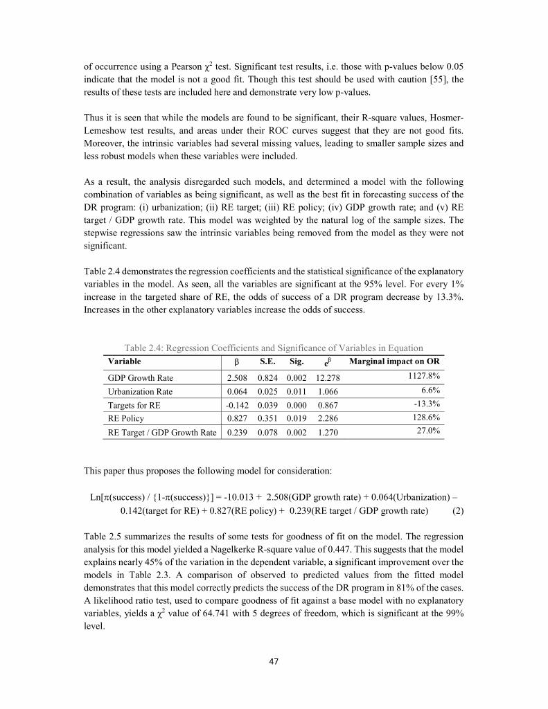
47

of occurrence using a Pearson χ2 test. Significant test results, i.e. those with p-values below 0.05 indicate that the model is not a good fit. Though this test should be used with caution [55], the results of these tests are included here and demonstrate very low p-values. Thus it is seen that while the models are found to be significant, their R-square values, Hosmer-Lemeshow test results, and areas under their ROC curves suggest that they are not good fits. Moreover, the intrinsic variables had several missing values, leading to smaller sample sizes and less robust models when these variables were included. As a result, the analysis disregarded such models, and determined a model with the following combination of variables as being significant, as well as the best fit in forecasting success of the DR program: (i) urbanization; (ii) RE target; (iii) RE policy; (iv) GDP growth rate; and (v) RE target / GDP growth rate. This model was weighted by the natural log of the sample sizes. The stepwise regressions saw the intrinsic variables being removed from the model as they were not significant. Table 2.4 demonstrates the regression coefficients and the statistical significance of the explanatory variables in the model. As seen, all the variables are significant at the 95% level. For every 1% increase in the targeted share of RE, the odds of success of a DR program decrease by 13.3%. Increases in the other explanatory variables increase the odds of success.

Table 2.4: Regression Coefficients and Significance of Variables in Equation Variable S.E. Sig. e Marginal impact on OR

GDP Growth Rate 2.508 0.824 0.002 12.278 1127.8%

Urbanization Rate 0.064 0.025 0.011 1.066 6.6%

Targets for RE -0.142 0.039 0.000 0.867 -13.3% RE Policy 0.827 0.351 0.019 2.286 128.6%

RE Target / GDP Growth Rate 0.239 0.078 0.002 1.270 27.0%

This paper thus proposes the following model for consideration:

Ln[(success) / {1-(success)}] = -10.013 + 2.508(GDP growth rate) + 0.064(Urbanization) – 0.142(target for RE) + 0.827(RE policy) + 0.239(RE target / GDP growth rate) (2)

Table 2.5 summarizes the results of some tests for goodness of fit on the model. The regression analysis for this model yielded a Nagelkerke R-square value of 0.447. This suggests that the model explains nearly 45% of the variation in the dependent variable, a significant improvement over the models in Table 2.3. A comparison of observed to predicted values from the fitted model demonstrates that this model correctly predicts the success of the DR program in 81% of the cases. A likelihood ratio test, used to compare goodness of fit against a base model with no explanatory variables, yields a χ2 value of 64.741 with 5 degrees of freedom, which is significant at the 99% level.

48

Table 2.5: Model Fit and Explanatory Power Indicator Value R-Square (Nagelkerke) 0.447 Correctly predicted values 80.90% Likelihood ratio test P-value (χ2 = 64.741 with 5 df) ~0.000

One limitation of this model is the presence of some correlations among the explanatory variables. In particular, as expected, correlations are noted between ‘RE Target,’ ‘GDP growth,’ and ‘RE Target / GDP growth.’ However, the variance inflation factors (VIFs) of these variables all lie between 1.2 and 4.1, which are within acceptable limits. Further, removing any of these variables reduces the explanatory power of the model and does not greatly affect the remaining model coefficients. Thus it is preferable to retain them. The ROC curve is seen in Figure 2.1. In the figure, sensitivity (also called the true positive rate) measures the proportion of positives that are correctly identified as such. Specificity (the true negative rate) measures the proportion of negatives that are correctly identified as such, i.e. the percentage of unsuccessful DR programs that are correctly identified as not being successful. The area under this ROC curve is much higher than the initial models in Table 2.2, at 0.855.

Figure 2.1: ROC Curve for Base Model

2.3.2 Robustness against Alternatives A common practice is to compare the main model to close alternatives to examine how the main estimates of the regression coefficients behave when the regression model is modified. If the coefficients are not found to change significantly, they are determined to be robust and can be interpreted as the true causal effects of the associated explanatory variables. This plausibility and robustness is a good estimate of the structural validity of a regression model [56].

49

The current analysis therefore assesses the base model outlined above against several alternatives with different combinations of explanatory variables. In this paper, the base model is compared against the best three alternatives, chosen based on their overall significance and R-square. The results are summarized in Table 2.6 below.

Table 2.6: Comparing Models

* Variables are denoted by their corresponding numbering from Tables 2.1 and 2.2

Thus, it is seen that the base model has the highest R-square, the second highest proportion of correctly predicted values, and the greatest number of variables with meaningful odds ratios, without having too many correlations among explanatory variables. The Hosmer-Lemeshow test results for the different models are also included. While even the base model is not determined to be a very good fit, since it does well on the other indicators in Table 2.6 and is also shown to be a better fit than the alternatives under the Hosmer-Lemeshow statistics, this paper retains this model as the most relevant one for analysis and further discussion. Additional sensitivity analyses conducted upon this model are summarized in Appendix 2-B. 2.3.3 Caution in Interpreting the Results It should be noted that the analysis suggests a correlation between the variables, but does not imply the existence of a causal relationship. The results provided above are conditional upon (i) a small sample size; (ii) missing information in the underlying studies; (iii) limited diversity in the features of the DR programs; and (iv) varying levels of granularity of the socio-economic variables. Thus, there is a possibility that increasing the sample size and improving the underlying data may yield different results than those presented here. One way this study attempts to reduce these risks is by limiting the approach to relatively straightforward statistical analyses. Conversely, this paper also aims to highlight the need for improving data, by demonstrating that such a meta-analytical approach is feasible. Keeping these points in mind, the results in Section 2.3 are offered at least indicatively, if not definitively.

50

2.4 Discussion As noted in Section 2.3, we found that a number of different models partially explained the chances of success of DR programs, in addition to the base model proposed. These alternative models used different combinations of explanatory variables, and arrived at different regression coefficients with varying levels of significance. Though intrinsic variables such as duration of the study and the presence of automated load controls did appear to play a part in determining the success of the DR programs, the key finding is that extrinsic variables such as RE targets and policy, GDP growth rates, and urbanization were consistently statistically significant. Thus, even if the results in Section 2.3 are offered indicatively, they can yield a number of insights. First, a DR program is very likely to be successful where economic growth rates are higher. Studies have shown that infrastructure investment – including investment in energy infrastructure – leads to higher economic growth and, in some cases, that growth spurs investment [57,58,59]. It is thus possible that DR programs are more likely to be implemented, and consequently more likely to be successful, in regions with higher growth rates. Second, a DR program is more likely to be successful in urban environments. There might be two reasons for this: (i) the higher densities of populations and electricity infrastructures in urban areas may create economies of scale and reduce the costs of – and increase the needs for – such programs; and (ii) urban consumers might be slightly more aware of energy and environmental issues [60,61,62]. Third, a DR program is less likely to be successful where national RE targets are high. We are not certain of the reasons behind this, but it is also conversely more likely to be successful when a strong RE policy exists. This could be because a strong RE policy may signal governmental commitment towards promoting RE and energy security, and may be associated with strong incentives and / or mandates, either to utility companies to deploy such programs, or to consumers to adopt them. Fourth, there is some inverse interaction between the national RE target and the GDP growth rates in determining the success of a DR program. While a relationship between the RE targets and GDP growth rates may make sense due to associated infrastructure requirements, the interaction term in this analysis may be more relevant for moderating the main effects. To contextualize these results within electricity consumption literature, a study in Saudi Arabia [63] that used auto-regression and causality testing found a bi-directional relationship between peak load and GDP, while empirical evidence from China [64] indicates a strong relationship between urbanization and energy use. Specific to DR programs, results from European projects [65] were unable to find significant correlations between socio-economic factors and response to pricing signals, though a survey of 15 US-based experiments [66] found a relationship between education and load shifting. This relationship was also observed in the Irish smart metering trial [15]. Education and income were however not found to be significant predictors of DR success in our study, which goes against expectations. This might be due to the limited size of the sample, and

51

their effects might be partly included in the role of urbanization in predicting the success of DR programs [67,68]. The omission of average temperatures and per capita electricity consumption patterns might similarly be on account of limited information. Alternatively, it is possible that temperatures do not affect DR programs because their effects are not significant or are offset by other factors. For instance, even during extreme weather events, reductions in electricity demand are possible due to the consequently higher dynamic prices [69]. Lastly, it is noteworthy that the final model does not include any intrinsic variables, though some of them were significant in other models we tested. However, this contradicts existing findings [12,13] on the role of enabling technologies and nature of enrolment in the success of DR. This is possibly because: (i) the intrinsic variables had many missing values, and their inclusion significantly reduced model sample sizes; and (ii) the DR programs were reasonably homogenous in structure – for instance most didn’t include automated load controls and most included voluntary (as opposed to automatic) enrolment options – possibly affecting the robustness of the regression models. These findings suggest the need for further contextual research, particularly while going beyond a single-case perspective. It is expected that future analyses, with more extensive data, would yield significant and robust models that include a mix of both intrinsic and extrinsic variables. These findings however have implications for shaping policy. The analysis suggests that the likelihood of success of a DR program is not just dependent on its structure, but also related to the socio-economic conditions under which it is implemented. Further study could argue a case to optimally structure DR programs such that they are most likely to succeed in their individual socio-economic environments. Perhaps this is most important in the case of developing countries, which do not yet possess adequate electricity infrastructure and present an opportunity to leapfrog traditional electricity markets. 2.5 Conclusion This paper conducted a meta-analysis, using a logistic regression approach, on 32 residential electricity demand response programs to analytically determine whether their likelihoods of success were correlated with the structures of and contexts surrounding the programs. The analysis found that the success appears to be correlated with the extent of urbanization in the region where the DR program is implemented, the renewable energy policy and targets, and the annual economic growth rates. While the sample size is small and the data is limited by missing values, the study offers the following guidance to increase the effectiveness of future DR programs: (i) Deploy DR programs in urban areas, particularly in faster-growing cities that are likely to have greater infrastructure spending; (ii) Align DR and electricity policy with renewable energy policies; and (iii) Couple electricity policy with wider economic policies and urban development planning, in order to also place it within the context of broader sustainable urban development. Future research may focus on addressing existing gaps by considering a wider set of DR programs for analysis; especially as such programs start to be implemented in developing countries. In

52

particular, it would be useful to look at the impacts of levels of awareness on demand flexibility and how this might affect the design of the programs. Specific to developing countries and emerging markets, it would also be useful to consider the impacts of DR programs on broader welfare considerations and other rebound effects.

53

Appendix 2-A

: Dem

and Response Initiatives and D

ata on Select Variables

Education

63.0%

63.0%

63.0%

78.5%

72.0%

61.0%

57.0%

63.0%

73.0%

80.0%

63.0%

52.0%

48.2%

89.0%

-

89.0%

Year

2020

2020

2020

2020

2020

2050

2020

2020

2020

2020

2020

2030

2030

2030

2025

2025

RE Target

62.9

62.9

26.0

37.0

20.9

80.0

15.0

62.9

42.5

70.6

62.9

23.0

20.0

50.0

50.0

25.0

Year

2014

2014

2014

2014

2014

2014

2014

2014

2014

2014

2014

2014

2014

2014

2014

2014

RE Share

63.3

63.3

33.4

10.0

13.4

28.2

7.0

63.3

22.7

70.0

63.3

12.2

11.1

24.4

31.2

11.5

Electricity Consumption

13870

13870

5159

6821

7967

7019

5407

13870

5702

8513

13870

7836

3762

7187

15519

12033

Urban %

86%

86%

26%

100%

98%

100%

83%

86%

63%

100%

100%

100%

56%

100%

82%

82%

GDP Growth

4.1%

4.1%

0.8%

2.0%

1.4%

1.7%

2.3%

4.1%

7.8%

0.9%

4.1%

0.5%

6.9%

2.4%

1.1%

2.4%

GDP per Capita

50273

29214

34011

44433

36269

42994

43734

50273

51289

41772

89989

22558

16526

48525

41849

59472

Sample

918

95

1446

77

186

41

2002

50

1964

775

400

88

236

8609

112642

10847

Success (Y=1)

0

1

0

1

0

1

1

1

1

1

1

1

1

1

1

1

Country

Sweden

Sweden

Italy

Netherlands

Belgium

Germany

Britain

Sweden

Ireland

Austria

Sweden

Japan

China

USA

Canada

USA

Study

Broberg and Persson [33]

Bartusch and Alvehag [38]

Torriti [36]

Kobus et [70]

D’hulst et al. [71]

Stamminger and Anstett [72]

Fell et al. [37]

Bartusch et al. [73]

Carroll et al. [74]

Schleich et al. [75]

Campillo et al. [76]

Kato et al. [77]

He et al. [30]

George and Toyama [78]

Faruqui et al. [79]

Becker [69]

54

Education

89.0%

89.0%

67.0%

80.0%

73.0%

89.0%

76.0%

57.0%

89.0%

76.0%

57.0%

80.0%

-

20.0%

87.0%

61.0%

Year

2030

2025

2020

2025

2020

2022

2020

2020

2032

2020

-

2025

2050

2030

2020

2050

RE Target

50.0

25.0

62.9

90.0

42.5

20.0

67.5

15.0

50.0

67.5

-

90.0

93.0

21.0

23.0

80.0

Year

2014

2014

2014

2013

2014

2014

2014

2014

2015

2014

2014

2013

2014

2010

2015

2014

RE Share

24.4

11.5

63.3

75.0

22.7

17.1

69.2

7.0

12.0

69.2

17.8

75.0

59.0

0.0

14.6

28.2

Electricity Consumption

7187

12033

13870

9084

5702

12129

23326

5407

21275

23326

4182

9084

15519

4326

10134

7019

Urban %

97%

100%

100%

100%

63%

100%

80%

100%

100%

80%

63%

100%

82%

100%

100%

75%

GDP Growth

2.4%

2.4%

4.1%

3.4%

7.8%

2.4%

1.6%

2.3%

2.4%

1.6%

2.3%

3.4%

1.1%

1.3%

2.3%

1.7%

GDP per Capita

61924

61236

36388

48447

51289

60751

74735

56233

77893

74735

26070

48089

40541

2803

51949

41219

Sample

457

590

33

332

1

878

295

1119

857

312

34779

63

1245

73

53

260

Success (Y=1)

1

1

0

0

1

1

1

1

1

0

1

1

1

1

0

0

Country

USA

USA

Sweden

New Zealand

Ireland

USA

Norway

Britain

USA

Norway

N. Ireland

New Zealand

Canada

South Africa

Australia

Germany

Study

Herter [80]

Allcott [81]

Nilsson et al. [82]

Thorsnes et al. [83]

Finn et al. [84]

Faruqui and Sergici [85]

Ericson [86]

Carmichael et al. [87]

Wolak [88]

Ericson [89]

Gans et al. [90]

Gyamfi and Krumdieck [91]

Woo et al. [92]

Thondhlana and Kua [31]

Hall et al. [93]

Alpenergy – VPS Allgau [94]

55

Appendix 2-B: Additional Sensitivity Analyses 2-B.1 Tests for Effect Heterogeneity We conduct additional sensitivity analyses on the proposed model, to check for the presence of heterogeneity in effects, and to also guard against the presence of confounding variables and Simpson’s paradox – in which a consistent effect in underlying studies disappears or reverses when studies are combined. We do this via two statistical tests, to estimate the model’s Cochran’s Q and I2 values. Cochran’s Q is a non-parametric test to examine the null hypothesis that all studies have the same effect on the population i.e. they yield consistent results. The test looks at the differences between observed effects for the studies and the pooled effect estimate. The test statistic is obtained by adding the squared deviations of each study's estimate from the overall meta-analytic estimate, weighting each study's contribution the same as in the meta-analysis. P-values are obtained by comparing the statistic with a χ2 distribution with (k-1) degrees of freedom, where k is the number of studies [95,96]. However, the Q test only indicates the presence versus the absence of heterogeneity; it does not report on the extent of such heterogeneity. The I2 index on the other hand describes the percentage of total variation across studies that is due to heterogeneity rather than chance. It measures the extent of true heterogeneity dividing the difference between the result of the Q test and its degrees of freedom by the Q value itself, and multiplied by 100 [96]. An I2 value above 50% indicates heterogeneity, while negative values are treated as being equivalent to 0% [95,96]. We note that the Cochran Q value of our model is 9.816 at 30 degrees of freedom, yielding a p-value of 0.9998. Thus we do not reject the null hypothesis of homogeneity. Further, the I2 value is -2.056, which is treated as 0%, and we thus conclude that there is no observed heterogeneity in the effects and it is appropriate to pool these studies in a meta-analysis. 2-B.2 Checking for Sample Outliers We further test the model and the parameter estimates by omitting two studies from the sample: those from Canada [79] and Northern Ireland [90]. These studies have significantly larger sample sizes than the other studies in the meta-analysis (112,642 and 34,779 respectively) and could be perceived as outliers, creating a risk of disproportionately affecting the results. To some extent, we have already mitigated against this risk in our model by weighting the studies by the natural logarithms of their sample sizes, rather than the sample sizes themselves – potentially creating a situation whereby these two studies are actually underrepresented – and note that the results from larger studies such as these might well be considered as more representative of actual effects. However, the results of a logistic regression, with the sample predictor variables as in our main model, but without these two studies, is shown below in Table 2-B.1.

56

Table 2-B.1: Model Comparisons with Omissions from Sample Variable Original With Two Studies Omitted

Sig. Impact on OR

Sig. Impact on OR

GDP Growth Rate 2.508 0.002 1127.8% 2.169 0.008 875.0% Urbanization Rate 0.064 0.011 6.6% 0.062 0.010 6.4% Targets for RE -0.142 0.000 -13.3% -0.125 0.001 -11.8% RE Policy 0.827 0.019 128.6% 0.719 0.045 105.3% RE Target / GDP 0.239 0.002 27.0% 0.202 0.009 22.4% R-Square 0.447 0.431 Hosmer-Lemeshow 0.030 0.003

It is seen that though the R-square and Hosmer-Lemeshow values indicate a somewhat poorer model fit without the two studies, the relative effect sizes and their statistical significances are almost unchanged. We thus conclude that the model was not significantly skewed by any outliers.

57

References [1] [Dataset] Eurostat. Share of energy from renewable sources, http://appsso.eurostat.ec.europa.eu/nui/show.do?dataset=nrg_ind_335a&lang=en [accessed 25.07.2017] [2] Power-technology.com. The true cost of energy storage, http://www.power-technology.com/features/featurethe-true-cost-of-energy-storage-4872402/ [accessed 07.12.2016] [3] Eurelectric. (2017). Dynamic pricing in electricity supply. Eurelectric. http://www.eurelectric.org/media/309103/dynamic_pricing_in_electricity_supply-2017-2520-0003-01-e.pdf [4] Torriti, J., Hassan, M. G., & Leach, M. (2010). Demand response experience in Europe: Policies, programmes and implementation. Energy, 35(4), 1575–1583. https://doi.org/10.1016/j.energy.2009.05.021 [5] DNV.GL, KEMA Consulting. (2014). Integration of renewable energy in Europe. European Commission. https://ec.europa.eu/energy/sites/ener/files/documents/201406_report_renewables_integration_europe.pdf [6] SEDC. (2017). Explicit demand response in Europe – Mapping the markets 2017. SEDC. http://www.smartenergydemand.eu/wp-content/uploads/2017/04/SEDC-Explicit-Demand-Response-in-Europe-Mapping-the-Markets-2017.pdf [7] European Commission. Commission proposes new rules for consumer centered clean energy transition, https://ec.europa.eu/energy/en/news/commission-proposes-new-rules-consumer-centred-clean-energy-transition [accessed 28.07.2017] [8] Joint Research Center. Smart grid projects map, http://ses.jrc.ec.europa.eu/sites/ses.jrc.ec.europa.eu/files/u24/2014/project_maps_28_april_2014.html [accessed 26.07.2017] [9] US Department of Energy. Smart grid demonstration program, https://www.smartgrid.gov/recovery_act/overview/smart_grid_demonstration_program.html [accessed 26.07.2017] [10] Gyamfi, S., Krumdieck, S., & Urmee, T. (2013). Residential peak electricity demand response - Highlights of some behavioural issues. Renewable and Sustainable Energy Reviews, 25, 71–77. https://doi.org/10.1016/j.rser.2013.04.006 [11] Faruqui, A., & George, S. (2005). Quantifying customer response to dynamic pricing. Electricity Journal, 18(4), 53–63. https://doi.org/10.1016/j.tej.2005.04.005 [12] Brent, D. A., Friesen, L., Gangadharan, L., & Leibbrandt, A. (2016). Behavioral insights from field experiments in environmental economics. Monash Business School, discussion paper 34/16. https://www.monash.edu/__data/assets/pdf_file/0009/926199/3416behavioralbrentfriesengangadharanliebbrandt.pdf

58

[13] US Department of Energy. Consumer behavior studies, https://www.smartgrid.gov/recovery_act/overview/consumer_behavior_studies.html [accessed 27.07.2017] [14] Kessels, K.; Kraan, C.; Karg, L.; Maggiore, S.; Valkering, P.; Laes, E. (2016). Fostering Residential Demand Response through Dynamic Pricing Schemes: A Behavioural Review of Smart Grid Pilots in Europe. Sustainability, 8(9), 929. http://www.mdpi.com/2071-1050/8/9/929 [15] Irish Commission for Energy Regulation. (2011). Electricity smart metering customer behavior trials findings report. CER. https://www.cru.ie/wp-content/uploads/2011/07/cer11080ai.pdf [16] Muratori, M., Schuelke-Leech, B. A., & Rizzoni, G. (2014). Role of residential demand response in modern electricity markets. Renewable and Sustainable Energy Reviews, 33, 546–553. https://doi.org/10.1016/j.rser.2014.02.027 [17] Cosmo, V. Di, & O’Hora, D. (2017). Nudging electricity consumption using TOU pricing and feedback: evidence from Irish households. Journal of Economic Psychology, 61, 1–14. https://doi.org/10.1016/j.joep.2017.03.005 [18] Flaim, T., Neenan, B., & Robinson, J. (2013). Pilot paralysis: Why dynamic pricing remains over-hyped and underachieved. Electricity Journal, 26(4), 8–21. https://doi.org/10.1016/j.tej.2013.04.002 [19] Stromback, J., Dromacque, C., & Yassin, M. H. (2011). The potential of smart meter enabled programs to increase energy and systems efficiency: A mass pilot comparison. VaasaETT. http://esmig.eu/sites/default/files/2011.10.12_empower_demand_report_final.pdf [20] Hobman, E. V., Frederiks, E. R., Stenner, K., & Meikle, S. (2016). Uptake and usage of cost-reflective electricity pricing: Insights from psychology and behavioural economics. Renewable and Sustainable Energy Reviews. https://doi.org/10.1016/j.rser.2015.12.144 [21] Faruqui, A., & Sergici, S. (2013). Arcturus: International Evidence on Dynamic Pricing. The Electricity Journal, 26(7), 55–65. https://doi.org/10.1016/j.tej.2013.07.007 [22] Faruqui, A., Sergici, S., & Sharif, A. (2010). The impact of informational feedback on energy consumption-A survey of the experimental evidence. Energy, 35(4), 1598–1608. https://doi.org/10.1016/j.energy.2009.07.042 [23] Comprehensive Meta-Analysis. Why perform a meta-analysis, https://www.meta-analysis.com/pages/why_do.php [accessed 04.11.2016] [24] Tatsioni, A., & Ioannidis, J. P. A. (2008). Meta-analysis. International Encyclopedia of Public Health. https://doi.org/10.1016/B978-012373960-5.00341-5 [25] Group, N. M. C. (2014). Preoperative chemotherapy for non-small-cell lung cancer: a systematic review and meta-analysis of individual participant data. Lancet (London, England), 383(9928), 1561–71. https://doi.org/10.1016/S0140-6736(13)62159-5 [26] Chrusciel, P., Sahebkar, A., Rembek-Wieliczko, M., Serban, M.-C., Ursoniu, S., Mikhailidis, D. P., … Banach, M. (2016). Impact of statin therapy on plasma adiponectin concentrations: A

59

systematic review and meta-analysis of 43 randomized controlled trial arms. Atherosclerosis, 253, 194 – 208. https://doi.org/10.1016/j.atherosclerosis.2016.07.897 [27] Sundt, S., & Rehdanz, K. (2015). Consumers’ willingness to pay for green electricity: A meta-analysis of the literature. Energy Economics, 51, 1–8. https://doi.org/10.1016/j.eneco.2015.06.005 [28] Mattmann, M., Logar, I., & Brouwer, R. (2016). Wind power externalities: A meta-analysis. Ecological Economics, 127, 23–36. https://doi.org/10.1016/j.ecolecon.2016.04.005 [29] Van Der Kroon, B., Brouwer, R., & Van Beukering, P. J. H. (2013). The energy ladder: Theoretical myth or empirical truth? Results from a meta-analysis. Renewable and Sustainable Energy Reviews, 20, 504–513. https://doi.org/10.1016/j.rser.2012.11.045 [30] He, Y., Wang, B., Wang, J., Xiong, W., & Xia, T. (2012). Residential demand response behavior analysis based on Monte Carlo simulation: The case of Yinchuan in China. Energy, 47(1), 230–236. https://doi.org/10.1016/j.energy.2012.08.046 [31] Thondhlana, G., & Kua, H. W. (2016). Promoting household energy conservation in low-income households through tailored interventions in Grahamstown, South Africa. Journal of Cleaner Production, 131, 327–340. https://doi.org/10.1016/j.jclepro.2016.05.026 [32] Filippini, M. (2011). Short- and long-run time-of-use price elasticities in Swiss residential electricity demand. Energy Policy. https://doi.org/10.1016/j.enpol.2011.06.002 [33] Broberg, T., & Persson, L. (2016). Is our everyday comfort for sale? Preferences for demand management on the electricity market. Energy Economics, 54, 24–32. https://doi.org/10.1016/j.eneco.2015.11.005 [34] Routes North. Cost of living in Sweden, https://www.routesnorth.com/planning-your-trip/cost-of-living-in-sweden/#Utilities [accessed 11.06.2019] [35] Numbeo. Cost of living in Sweden, https://www.numbeo.com/cost-of-living/country_result.jsp?country=Sweden [accessed 11.06.2019] [36] Torriti, J. (2012). Price-based demand side management: Assessing the impacts of time-of-use tariffs on residential electricity demand and peak shifting in Northern Italy. Energy, 44(1), 576–583. https://doi.org/10.1016/j.energy.2012.05.043 [37] Fell, M. J., Shipworth, D., Huebner, G. M., & Elwell, C. A. (2015). Public acceptability of domestic demand-side response in Great Britain: The role of automation and direct load control. Energy Research and Social Science, 9, 72–84. https://doi.org/10.1016/j.erss.2015.08.023 [38] Bartusch, C., & Alvehag, K. (2014). Further exploring the potential of residential demand response programs in electricity distribution. Applied Energy, 125, 39–59. https://doi.org/10.1016/j.apenergy.2014.03.054 [39] [Dataset] The World Bank. World development indicators: Towards a broader measure of national income, http://wdi.worldbank.org/table/4.10 [accessed 01.08.2017] [40] [Dataset] The World Bank. GDP per capita (current US$), http://data.worldbank.org/indicator/NY.GDP.PCAP.CD [accessed 28.11.2016]

60

[41] [Dataset] The World Bank. GDP growth (annual %), http://data.worldbank.org/indicator/NY.GDP.MKTP.KD.ZG [accessed 28.11.2016] [42] [Dataset] The World Bank. Urban population (% of total), http://data.worldbank.org/indicator/SP.URB.TOTL.in.zs [accessed 28.11.2016] [43] World Weather Online. Various pages, https://www.worldweatheronline.com/ [accessed 24.11.2016] [44] [Dataset] The World Bank. Electric power consumption (kWh per capita) http://data.worldbank.org/indicator/EG.USE.ELEC.KH.PC [accessed 28.11.2016] [45] REN21. (2016). Renewables 2016 global status report. REN21. http://www.ren21.net/wp-content/uploads/2016/06/GSR_2016_Full_Report.pdf [46] [Dataset] The World Bank. Gross enrolment ratio, tertiary, both sexes (%), http://data.worldbank.org/indicator/SE.TER.ENRR [accessed 28.11.2016] [47] Faruqui A., Sergici S., & Palmer J. (2010). The impact of dynamic pricing on low income customers. IEE Whitepaper. http://www.edisonfoundation.net/IEE/Documents/IEE_LowIncomeDynamicPricing_0910.pdf [48] Bayar, Y., & Özel, H. A. (2014). Electricity Consumption and Economic Growth in Emerging Economies. Journal of Knowledge Management, Economics and Information Technology, 4(2), 118. http://www.scientificpapers.org/knowledge-management/electricity-consumption-and-economic-growth-in-emerging-economies/ [49] Liddle, B., & Lung, S. (2014). Might electricity consumption cause urbanization instead? Evidence from heterogeneous panel long-run causality tests. Global Environmental Change, 24(1), 42–51. https://doi.org/10.1016/j.gloenvcha.2013.11.013 [50] Qiu, Y., Colson, G., & Wetzstein, M. E. (2017). Risk preference and adverse selection for participation in time-of-use electricity pricing programs. Resource and Energy Economics, 47, 126–142. https://doi.org/10.1016/j.reseneeco.2016.12.003 [51] Bouckaert, S., Mazauric, V., & Maïzi, N. (2014). Expanding renewable energy by implementing demand response. In Energy Procedia (Vol. 61, pp. 1844–1847). https://doi.org/10.1016/j.egypro.2014.12.226 [52] Breaking Energy. Can demand response programs help meet the renewable energy integration challenge? http://breakingenergy.com/2012/08/09/can-demand-response-programs-help-meet-the-renewable-energy-inte/ [accessed 11.01.2016] [53] Nelson, J. P., & Kennedy, P. E. (2009). The use (and abuse) of meta-analysis in environmental and natural resource economics: as assessment. Environmental Resource Economics, 42, 345–377. https://doi.org/10.1007/s10640-008-9253-5 [54] Hosmer, D. W., & Lemeshow, S. (2000). Applied Logistic Regression. Wiley Series in Probability and Statistics (Vol. 23). Hoboken, NJ, USA: John Wiley & Sons, Inc. https://doi.org/10.1002/0471722146

61

[55] Hosmer, D. W., Hosmer, T., Le Cessie, S., & Lemeshow, S. (1997). A comparison of goodness-of-fit tests for the logistic regression model. Statistics in Medicine, 16(9), 965–980. https://doi.org/10.1002/(SICI)1097-0258(19970515)16:9<965::AID-SIM509>3.0.CO;2-O [56] Lu, X., & White, H. (2014). Robustness checks and robustness tests in applied economics. Journal of Econometrics, 178(Part 1), 194–206. https://doi.org/10.1016/j.jeconom.2013.08.016 [57] Ilesanmi, K. D., & Tewari, D. D. (2017). Energy consumption, human capital investment and economic growth in South Africa: a vector error correction model analysis. OPEC Energy Review, 41(1), 55–70. https://doi.org/10.1111/opec.12094 [58] Lawson, S., & Dragusanu, R. (2008). Building the world: Mapping infrastructure demand. Goldman Sachs Global Economics Paper, 166. http://www.goldmansachs.com/our-thinking/archive/archive-pdfs/infrastructure-building-the-world.pdf [59] European Commission. (2014). Infrastructure in the EU: Developments and impact on growth. EC Occasional Papers, 203. http://ec.europa.eu/economy_finance/publications/occasional_paper/2014/pdf/ocp203_en.pdf [60] European Commission. (2014). Attitudes of European citizens towards the environment. Eurobarometer Report, 416. https://doi.org/10.2779/25662 [61] Berenguer, J., Corraliza, J. A., & Martin, R. (2005). Rural-Urban differences in environmental concern, attitudes, and actions. European Journal of Psychological Assessment, 21(2), 128–138. https://doi.org/10.1027/1015-5759.21.2.128 [62] Panigrahi, A., (2015). Comparative study of green marketing’s effect on urban consumers and rural consumers. Unpublished. https://papers.ssrn.com/sol3/papers.cfm?abstract_id=2686805 [63] Alsaedi, Y.H., & Tularam, G.A. (2019). The relationship between electricity consumption, peak load and GDP in Saudi Arabia: A VAR analysis. Mathematics and Computers in Simulation. https://doi.org/10.1016/j.matcom.2019.06.012 [64] Sheng, P., & Guo, X. (2018). Energy consumption associated with urbanization in China: Efficient- and inefficient-use. Energy. https://doi.org/10.1016/j.energy.2018.09.161 [65] Advanced FP7. Project homepage, https://www.advancedfp7.eu/ [accessed 14.06.2019] [66] Faruqui, A., & Sergici, S. (2010). Household response to dynamic pricing of electricity: A survey of 15 experiments. Journal of Regulatory Economics. https://doi.org/10.1007/s11149-010-9127-y [67] The Economic Times. Big gap in per capita income in urban and rural areas, https://economictimes.indiatimes.com/news/politics-and-nation/big-gap-in-per-capita-income-in-urban-and-rural-areas/articleshow/52208067.cms [accessed 21.06.2019] [68] Statista. Annual per capita disposable income of rural and urban households in China from 1990 to 2017, https://www.statista.com/statistics/259451/annual-per-capita-disposable-income-of-rural-and-urban-households-in-china/ [accessed 21.06.2019] [69] Becker, D. (2015). Baby, It’s Cold Outside: 2014 Polar Vortex Impacts on Residential Dynamic Electricity Pricing Programs. In International Energy Program Evaluation Conference

62

2015. http://www.elevateenergy.org/wp/wp-content/uploads/2014PolarVortexImpactsResidentialDynamicPricing.pdf [70] Kobus, C. B. A., Klaassen, E. A. M., Mugge, R., & Schoormans, J. P. L. (2015). A real-life assessment on the effect of smart appliances for shifting households’ electricity demand. Applied Energy, 147, 335–343. https://doi.org/10.1016/j.apenergy.2015.01.073 [71] D’hulst, R., Labeeuw, W., Beusen, B., Claessens, S., Deconinck, G., & Vanthournout, K. (2015). Demand response flexibility and flexibility potential of residential smart appliances: Experiences from large pilot test in Belgium. Applied Energy, 155, 79–90. https://doi.org/10.1016/j.apenergy.2015.05.101 [72] Stamminger, R., & Anstett, V. (2013). The Effect of Variable Electricity Tariffs in the Household on Usage of Household Appliances. Smart Grid and Renewable Energy, 4, 353–365. https://doi.org/10.4236/sgre.2013.44042 [73] Bartusch, C., Wallin, F., Odlare, M., Vassileva, I., & Wester, L. (2011). Introducing a demand-based electricity distribution tariff in the residential sector: Demand response and customer perception. Energy Policy, 39(9), 5008–5025. https://doi.org/10.1016/j.enpol.2011.06.013 [74] Carroll, J., Lyons, S., & Denny, E. (2014). Reducing household electricity demand through smart metering: The role of improved information about energy saving. Energy Economics, 45, 234–243. https://doi.org/10.1016/j.eneco.2014.07.007 [75] Schleich, J., Klobasa, M., Gölz, S., & Brunner, M. (2013). Effects of feedback on residential electricity demand-findings from a field trial in Austria. Energy Policy, 61, 1097–1106. https://doi.org/10.1016/j.enpol.2013.05.012 [76] Campillo, J., Dahlquist, E., Wallin, F., & Vassileva, I. (2016). Is real-time electricity pricing suitable for residential users without demand-side management? Energy, 109, 310–325. https://doi.org/10.1016/j.energy.2016.04.105 [77] Kato, T., Tokuhara, A., Ushifusa, Y., Sakurai, A., Aramaki, K., & Maruyama, F. (2016). Consumer responses to critical peak pricing: Impacts of maximum electricity-saving behavior. Electricity Journal, 29(2), 12–19. https://doi.org/10.1016/j.tej.2016.02.002 [78] George, S., & Toyama, N. (2015). Final Results from SMUD’s SmartPricing Options Pilot. In International Energy Program Evaluation Conference 2015. http://www.iepec.org/wp-content/uploads/2015/papers/029.pdf [79] Faruqui, A., Lessem, N., Sergici, S., Mountain, D., Denton, F., & Spencer, B. (2015). Analysis of Ontario’s Full Scale Roll-out of TOU Rates. In International Energy Program Evaluation Conference 2015. http://www.iepec.org/wp-content/uploads/2015/papers/030.pdf [80] Herter, K. (2007). Residential implementation of critical-peak pricing of electricity. Energy Policy, 35(4), 2121–2130. https://doi.org/10.1016/j.enpol.2006.06.019 [81] Allcott, H. (2011). Rethinking real-time electricity pricing. Resource and Energy Economics, 33(4), 820–842. https://doi.org/10.1016/j.reseneeco.2011.06.003

63

[82] Nilsson, A., Bergstad, C. J., Thuvander, L., Andersson, D., Andersson, K., & Meiling, P. (2014). Effects of continuous feedback on households’ electricity consumption: Potentials and barriers. Applied Energy, 122, 17–23. https://doi.org/10.1016/j.apenergy.2014.01.060 [83] Thorsnes, P., Williams, J., & Lawson, R. (2012). Consumer responses to time varying prices for electricity. Energy Policy, 49, 552–561. https://doi.org/10.1016/j.enpol.2012.06.062 [84] Finn, P., O’Connell, M., & Fitzpatrick, C. (2013). Demand side management of a domestic dishwasher: Wind energy gains, financial savings and peak-time load reduction. Applied Energy, 101, 678–685. https://doi.org/10.1016/j.apenergy.2012.07.004 [85] Faruqui, A., & Sergici, S. (2011). Dynamic pricing of electricity in the mid-Atlantic region: Econometric results from the Baltimore gas and electric company experiment. Journal of Regulatory Economics, 40(1), 82–109. https://doi.org/10.1007/s11149-011-9152-5 [86] Ericson, T. (2011). Households’ self-selection of dynamic electricity tariffs. Applied Energy, 88(7), 2541–2547. https://doi.org/10.1016/j.apenergy.2011.01.024 [87] Carmichael, R., Schofield, J., Woolf, M., Bilton, M., Ozaki, R., & Strbac, G. (2014). Residential consumer attitudes to time-varying pricing. “Low Carbon London” LCNF project, Report A2. http://innovation.ukpowernetworks.co.uk/innovation/en/Projects/tier-2-projects/Low-Carbon-London-(LCL)/Project-Documents/LCL%20Learning%20Report%20-%20A2%20-%20Residential%20consumer%20attitudes%20to%20time%20varying%20pricing.pdf [88] Wolak, F. A. (2011). Do residential customers respond to hourly prices? Evidence from a dynamic pricing experiment. American Economic Review, 101, 83–87. https://doi.org/10.1257/aer.101.3.83 [89] Ericson, T. (2006). Time-differentiated pricing and direct load control of residential electricity consumption. Statistics Norway, Discussion Paper No. 461. http://www.ssb.no/a/publikasjoner/pdf/DP/dp461.pdf [90] Gans, W., Alberini, A., & Longo, A. (2013). Smart meter devices and the effect of feedback on residential electricity consumption: Evidence from a natural experiment in Northern Ireland. Energy Economics, 36, 729–743. https://doi.org/10.1016/j.eneco.2012.11.022 [91] Gyamfi, S., & Krumdieck, S. (2011). Price, environment and security: Exploring multi-modal motivation in voluntary residential peak demand response. Energy Policy, 39(5), 2993–3004. https://doi.org/10.1016/j.enpol.2011.03.012 [92] Woo, C. K., Li, R., Shiu, A., & Horowitz, I. (2013). Residential winter kWh responsiveness under optional time-varying pricing in British Columbia. Applied Energy, 108, 288–297. https://doi.org/10.1016/j.apenergy.2013.03.042 [93] Hall, N. L., Jeanneret, T. D., & Rai, A. (2016). Cost-reflective electricity pricing: Consumer preferences and perceptions. Energy Policy, 95, 62–72. https://doi.org/10.1016/j.enpol.2016.04.042 [94] S3C. Alpenergy – VPS Allgau, http://www.s3c-project.eu/News/40/AlpEnergyVPSAllgu.html [accessed 13.10.2016]

64

[95] Higgins, J. P. T., Thompson, S. G., Deeks, J. J., & Altman, D. G. (2003). Measuring inconsistency in meta-analyses. BMJ (Clinical Research Ed.). https://doi.org/10.1136/bmj.327.7414.557 [96] Huedo-Medina, T. B., Sánchez-Meca, J., Marín-Martínez, F., & Botella, J. (2006). Assessing heterogeneity in meta-analysis: Q statistic or I 2 Index? Psychological Methods. https://doi.org/10.1037/1082-989X.11.2.193

65

A Quantile Analysis of Constituent Factors 3. Chapter based upon: Srivastava, A., Van Passel, S., & Laes, E. (2019). Dissecting demand response: A quantile analysis of flexibility, household attitudes, and demographics. Energy Research and Social Science, 52, 169-180. Available at https://doi.org/10.1016/j.erss.2019.02.011 3.1 Introduction 3.1.1 Demand Response The electricity sector is faced with two medium- to long-term challenges. First, it is a significant contributor to climate change, with nearly 30% of total greenhouse gas emissions coming from global electricity production [1]. At the same time, electricity consumption trends – coupled with an aging infrastructure – present a challenge for energy security. In Europe, various operating reserves9 exist to secure the supply of electricity. The primary reserve is used to maintain load frequency and avoid grid instability, the secondary reserve is used to alleviate imbalances, and the tertiary reserve is used to cope with significant imbalances and major congestion problems [2,3].

In its primary reserve alone, the interconnected European electricity market needs around 3 gigawatts (GW) of capacity [4]. The increasing share of renewable sources in electricity generation is a potential long-term solution for both, mitigating climate change and securing energy supplies. However, the generation of renewable electricity is intermittent in nature, while non-intermittent generation is expensive and storage technologies are still inefficient. Demand response (DR) programs are seen as a promising option for the integration of renewables [5], and as a cheaper alternative to the conventional generation that is currently used to ensure the security of energy supply [4]. DR programs aim to modify the demand patterns for electricity by encouraging its use during peak generation and discouraging its use at times when the load on the grid is highest. This modification of demand is typically achieved through the dynamic pricing of electricity based on the time of its use, or through the external control of appliance loads [6]. The European Commission (EC) estimates a total response potential of 160 GW by 2030, with 40% of the potential for peak load reductions coming from the residential sector [7]. It has thus unveiled a ‘Clean Energy for All Europeans’ proposal [8] which recommends greater customer access to dynamic pricing contracts, DR programs, smart metering systems, and information feedback. In line with this, DR is being promoted through enabling policy frameworks in many European countries, and DR programs are being increasingly tested and implemented in the residential sector10 [11].

9 An operating reserve is the reserve generating capacity available to the system operator, to meet demand in a short period of time, in case there is a sudden disruption to the power supply or an extensive blackout 10 A list of European smart grid projects is available with the EC’s Joint Research Center [9], while a list of demonstration projects supported by the US government is available at the US Department of Energy [10]

66

Residential DR programs can however be more challenging to implement successfully, due to the limited price responsiveness of households [12]. There have consequently been a number of studies aimed at better understanding household response to – including user perceptions of and concerns with – DR programs. 3.1.2 Literature on Household Response to Demand Response Often, literature looks at response to DR from varying perspectives. On pricing, for instance, Bartusch et al. [13] found, relying on analysis of a pilot project and ten interviews, that households in Sweden do indeed act on the price signals of time-of-use (ToU) tariffs by decreasing demand in peak periods and shifting electricity use to off-peak periods, although three of the households had witnessed reductions in overall consumption because they had switched to heat pumps. From the perspective of information, Hall et al. [14] used focus groups – among a random sample of respondents with high rates of employment – to identify that households in Australia are open to ToU pricing, but want more information to understand the potential benefits of DR. Regarding privacy concerns, Muratori et al.’s [15] review of literature found that consumers are reluctant to allow external control of their appliances, and continue to have concerns about information sharing. Similarly, Darby and McKenna’s [16] review of 16 DR trials – focused mainly on ToU and real time pricing (RTP) – points to the need for customer education and attention to data privacy and security. Parag and Butbul [17] studied the interest among 554 non-representative pro-technology respondents in Israel in adopting smart home technologies using hierarchical linear regression and found that potential adopters value the perceived benefits of comfort and convenience over the risks associated with these technologies. Other studies have studied response from multiple perspectives in combination. An EC report found that consumer acceptance of smart appliances depends on the respective device; for instance, smart operation for washing machines and dishwashers is highly accepted. But key user concerns continue to include doubts about the safety of smart appliances, doubts about the maturity of the technology, and the fear of losing control over the operations of such appliances [18]. Brent et al. [19] review a number of artefactual field experiments in dynamic electricity pricing and state that price changes lead to greater conservation effects than moral and social arguments, that knowledge of consumption can maximize the effectiveness of time-varying pricing, and that enabling technology increases the effectiveness of such pricing. Consumer behavior studies undertaken by 10 utilities – using randomized control trials – under the US government’s Smart Grid Investment Grant program found, among others, that enrolment under opt-out approaches was significantly higher than under opt-in approaches due to status-quo effects, and that higher price ratios led to greater response [20]. Kessels et al. [21] studied the findings from nine European dynamic pricing pilot projects to conclude that dynamic pricing schemes should be simple to understand, with timely notifications of price changes, a considerable potential effect on the energy bill, and automated control. Existing research has also occasionally thrown up conflicting findings. For instance, Gyamfi et al. [12] reviewed pricing-based DR literature and found that a high fraction of households –

67

particularly the richer ones11 – did not respond to price signals. However, the Irish energy regulator [24] found through its smart metering behavioral trial among a representative sample that ToU tariffs did reduce electricity usage, and that higher-consuming households tended to deliver greater reductions. Muratori et al. [15] further found that shifting consumption may lead to steeper rebound peaks, while Cosmo and O’Hora [25], using difference-in-difference estimates, found that demand reductions in the Irish smart metering trial lasted beyond the peak period and that post-peak spikes in usage were not observed. Overall, Parrish et al. [26] found through a systematic review of 94 trials, surveys, and programs, that customer responses can vary considerably for many reasons and that because the picture is somewhat mixed, greater empirical evidence is needed, while Srivastava et al. [27] noted based on a meta-analysis of 32 DR programs that response may also be dependent on contextual socio-economic factors. In this context, Gyamfi et al. [12] suggest greater use of economic behavior-based approaches to overcome some of the challenges to achieving effective voluntary demand reductions. 3.1.3 Scope of Current Study A greater understanding of how user perceptions affect response is needed, in order to better design and implement DR programs in the future. This paper undertakes such an analysis, using a unique approach, by conducting an in-depth study of the heterogenous relationship between user perceptions – taking into account their attitudes towards factors such as information, privacy, control – and response. In this, it focuses on the Belgian region of Flanders. In addition to the European reserves, Belgium requires 600 megawatts (MW) in its strategic reserve, introduced to cover structural shortages in generation during the winter periods [28,29]. Separately, new legislation in Belgium is establishing the right for an independent aggregator to access consumers directly – this will help to provide an equal footing for all market actors; a good sign for the uptake of DR [11]. In recognition of these market changes at the national and European levels, Belgium has also hosted various smart grid projects [9], largely international and / or R&D undertakings. Among these, the only domestic DR demonstration – meant to test the feasibility of a broader rollout – was Linear, a smart grid trial in the region of Flanders that concluded in 2014 [30]. This paper analyzes the perceptions and behaviors of the households that had participated in the Linear field trial, to see how their attitudes and concerns relate to the flexibility they had offered during this trial. It employs the technique of quantile regressions to disaggregate participant responses to the trial and identify whether different levels of response were associated with different perceptions of and concerns with the project. Such a quantile regression approach has not often been used for electricity consumption analysis. Kaza [31] used a quantile regression analysis to show that while housing size matters for space conditioning, housing type has a more nuanced impact, and that the effects of various factors at the tails of the energy use distribution are substantially different than the average. Khanna et al. [32] conducted a quantile regression analysis of residential electricity consumption in China against socio-economic and demographic factors to 11 Richer households tend to consume greater amounts of electricity, as determined by for instance Vesterberg [22] and Silva et al. [23]

68

study the impacts of demand side management. Romero-Jordan et al. [33] found that in that Spanish context during the recent economic crisis, electricity consumption of medium-high income households was particularly responsive to price increases, whereas that of medium-low income households was more responsive to changes in income. However, no studies have used this approach to understand demand response from a behavioral perspective and thus guide the direction of the electricity market. By adopting this approach to not only dissect response, but also analyze this response in combination with users’ perceptions and attitudes, this paper provides more in-depth recommendations – offering unique perspectives drawn from an actual field trial – to inform a wider demand response rollout in the future. The contributions of this paper are then threefold: (i) It studies user responses and perceptions of a DR trial in combination; (ii) It undertakes a quantitative analysis of this DR trial, where previous studies have tended to study such trials qualitatively; and (iii) It applies the method of quantile regressions, for the first time in this field of study, to yield a more comprehensive analysis of the heterogenous relationship between response and perception, by demonstrating how some percentiles of response are more affected by specific attitudes than other percentiles. This article is set up as follows: Section 3.2 provides an introduction to the Linear project – from which we obtained our data – and lists the project findings. Section 3.3 outlines the research method as well as the design for obtaining and processing the data. Section 3.4 lists the statistical results from our regression analyses, while Section 3.5 offers an interpretation and discussion of these results. Section 3.6 concludes with recommendations. 3.2 The Linear Smart Grid Trial Linear was a demonstration project on smart grid technologies that ran for three years from 2011 until 2014, recruiting participants in three phases between 2011 and 2012, in the Belgian region of Flanders. It aimed to activate residential demand response to facilitate the integration of renewable energy sources in the network. One of the main project objectives was to develop the required technical solutions to realize a breakthrough in DR [34]. The field trial within the project ran for a year; it was based on voluntary participation, and 240 households were involved. The families that participated were already favorably disposed towards smart appliances and were thus not representative of the population. Further, Linear recruited families that lived in owned houses, rather than rentals and / or apartments. The average participating household had four members, lived in a house built after 1980, and owned at least one television and laptop [34]. The project report [34] states that the incomes of participants were higher than the Belgian monthly per capita of 3445 euros [35], although the actual sample average was not available to the authors. Despite their positive attitudes, participants were unwilling to run any financial risk in the project, and most households were not willing to replace their existing appliances with smart ones as long as they were still usable. Additional incentives were therefore developed in order to get more users on board. These incentives, such as rebates and free tablets, cannot be reproduced for a full market

69

deployment, which – aside from sample representativeness – was acknowledged as a typical limitation that might hinder a successful full-scale rollout [34]. The unrepresentativeness of the sample combined with the mix of incentives offered to participants suggests that the trial had low external validity. In the process, however, it did yield important lessons on the barriers to entry. The Linear trial split the participants in two broad groups (see Table 3.1); for each group a different reward system was tested. Of the 240 participating families, 54 were exposed to time-of-use electricity pricing – they were subject to six rate categories per day, and the prices in these categories were communicated the day before. These 54 were provided with home energy management systems, sub-metering plugs, smart meters, and displays to help them with insights into their consumption. The primary focus of the trial however was on the remaining 186 families. These families were provided with homes energy management systems and 445 postponable smart appliances – washing machines, dishwashers, and tumble dryers – such that most families had all three appliances;12&13 106 households were also equipped with smart meters. The 186 families received a fee of €1 per 40 hours of flexibility – defined by Linear as the number of hours within which the appliance had to start after being switched on, in order to finish by the time pre-set by the users – that they offered through these appliances [34].

Table 3.1: Linear Test Families Group Smart Meter No Smart Meter Smart Appliances 85 families 101 families

Time-of-use Tariffs 21 families 33 families

Source: Adapted from the Linear Consortium [31]

The trial found that the response to time-based pricing was weak, while the acceptance of smart appliances turned out to be much higher. In total, the participants in the second group offered 200,000 hours of flexibility with their 445 smart appliances, or an average of 450 hours per appliance across the year. There was no reported user fatigue, although technical issues were reported with the functionality of the appliances and the retrofitted communications architecture. Linear extrapolated the results of this field test to estimate that a full DR rollout in Belgium among white good appliances could lead to a maximum of 280 MW of flexibility being realized [34]. The Linear project also conducted user surveys before and after the one-year field trial, to gauge the acceptance of, and shifts in attitudes with regard to, smart appliances in a residential environment. These surveys were designed based on the technology acceptance model that has also been used in other literature [36], and they were designed while minimizing cognitive burden to

12 Data on the distribution of these appliances was not available 13 A limited number of households also received hot water buffers and electric vehicles; these were not considered in our analysis due to the small sample size

70

the respondents. The surveys focused on nine dimensions: (i) perceived safety, (ii) perceived maintained control, (iii) expected comfort maintenance, (iv) perceived expected costs, (v) perceived environmental friendliness, (vi) perceived ease of use, (vii) perceived usefulness, (vii) overall attitude, and (ix) intention to use / actual use of smart appliances. The dimension of overall attitude towards smart appliances was also based on survey questions, and was not an aggregate of the other eight dimensions. Each question in the survey required a Likert scale-type response, and mean scores were calculated for each dimension on a 5-point scale. The 155 responses received by the smart appliance users14 showed – as seen in Figure 3.1 – that participants’ attitudes towards smart appliances became slightly less favorable over the course of the trial, across all the dimensions measured. These drops were induced partly due to problems experienced during the field trial; for instance, 55.2% of the participants experienced poor functionality of the system. This point suggests that the trial implementation wasn’t completely successful, based on some dimensions. However, Linear concluded that the enthusiasm before the start of the field trial shifted to a more nuanced, yet still positive, opinion about the appliances by the end of the trial.

Figure 3.1: Mean Scores on Attitude Measurements Before (T1) and After (T2) Trial

Source: Unpublished Linear User Acceptance Report

In this way, Linear’s analysis provided initial insights into user attitudes regarding the field trial by aggregating the survey responses. This current paper complements and builds upon Linear’s findings by disaggregating these responses and coupling them with the results of the trial.

14 The results of the surveys are captured in an unpublished user acceptance (UA) report. The authors of this paper were able to access the UA report as well as a limited set of the underlying data, though they were not provided with the underlying methodology for assigning scores to the attitude measurements

1

2

3

4

5

Mea

n Sc

ore

T1 T2

71

3.3 Methods 3.3.1 Research Method: Quantile Regression The standard ordinary least squares (OLS) model is commonly used because of its advantages: it is easy to use and analyze, it has wide applicability, and it yields estimates that are unconditional. At the same time however, it has a number of inherent limitations. First, it summarizes the response across an entire dataset – thus assuming that one model is appropriate for the whole data – and cannot be customized to noncentral locations, which are often more interesting in a sample distribution than the central locations. Second, the model assumptions are often not realistic; for instance, sample distributions are often not normal and / or are homoscedastic. Third, the OLS model can be heavily influenced by the presence of a few outliers in the sample [37]. Conditional quantile modeling, or quantile regression (QR), replaces the least squares estimation of OLS with least absolute distance estimation, to estimate the relationships between a response and a set of covariates for specific quantiles (or percentiles) of the response distribution. While the linear regression model specifies the change in the conditional mean of the dependent variable, subject to a change in the covariates, the QR model specifies changes in its conditional quantile – where the 50th quantile is the median. Since multiple quantiles can be modeled, it is possible to get a more complete understanding of the response distribution. Further, since outliers can be isolated into the top or bottom quantiles, QR estimates are robust against them [37,38]. The pth quantile denotes that value of the response below which the proportion of the sample population is p. Thus, similar to a standard OLS model, which takes the form in Equation (1), a QR model, for the pth quantile, takes the form shown in Equation (2). Thus in the QR model, the coefficients are quantile-specific.

yi = β0 + β1x1i + … + βjxji + εi (1)

yi = β(p)0 + β(p)

1x1i + … + β(p)jxji +ε(p)

i (2) Where yi = Response variable for ith observation βj = Model coefficient for jth predictor variable xji = jth predictor variable for ith observation εi = Error term for ith observation However, while the OLS coefficients are determined by taking those values of the parameters that minimize the sum of squared residuals, the QR coefficients are determined by taking those values of the parameters that minimize the weighted sum of absolute residuals, as shown in Equation (3) below. This weighted sum gives asymmetric penalties for overprediction and underprediction, with asymmetry increasing as p approaches 0 or 1. It may be noted that the estimation of coefficients for each quantile regression is based on the weighted data of the whole sample, and not just the portion of the sample at that quantile [37].

72

∑ i:y≥x′β(p)| yi – β(p)

0 – β(p)1xi … – β(p)

jxji | + ∑ i:y<x′β

(1−p)| yi – β(p)0 – β(p)

1xi … – β(p)jxji | (3)

Unlike OLS, the QR coefficients do not have a closed-form solution, and Equation (3) is instead solved using linear optimization algorithms, such as the simplex method. However, the quantile regression estimator is asymptotically normally distributed [37]. 3.3.2 Research Design: Data and Pre-processing The underlying data from the Linear field trial was provided by VITO, the Flemish Institute for Technological Research. This data included, for each participating household, (i) demographics for the head of the family – age and gender, (ii) participation details, such as whether the participants were given smart appliances or on ToU tariffs, (iii) responses to the pre-trial and post-trial attitude surveys, and (iv) responses to the field trial, in terms of hours of flexibility and bonuses awarded. However, much other data from the trial, particularly about the sample constituents, was not disclosed to us for confidentiality reasons. The authors processed this data as follows: (i) translated the data from Flemish Dutch into English; (ii) compiled and cross-referenced the data from across various databases provided by VITO; (iii) filtered out questions that were open-ended, rather than numerical, scaled, or binary in response; (iv) removed questions that were unrelated to user behavior or response; and (v) coded the Likert scale responses into categorical variables to enable statistical analysis. The analysis was conducted in the statistical software R. Since the focus of the Linear trial was on smart appliance users – the sample of users on ToU tariffs was smaller, and the response to smart appliances turned out to be stronger in the field trial – this analysis also focuses on the same group, and the sample thus consisted of the 155 smart appliances users who had completed Linear’s user surveys. The total hours of flexibility offered by each household across the duration of the trial was assigned as the response variable15. Existing literature – such as the studies featured in Section 3.1.2 – suggests that household response to, and even willingness to participate in, DR programs is related to factors such as pricing considerations, awareness of the benefits of DR, presence of information feedback systems such as smart meters or in-home usage displays, privacy concerns relating to smart appliances and meters, confidence in the associated technologies, impacts on convenience relating to the operability of appliances, and respondents’ psychological profiles, such as their attitudes towards the environment and preferences for loss and / or risk aversion. Based on the literature, the analysis for this paper assumed response to be a generalized function of the following:

Response = f (Pricing, Knowledge, Feedback, Privacy, Technology, Convenience, Respondent profile) (4)

15 Flexibility was calculated within the Linear trial as the number of hours within which the appliance had to start after being switched on, in order to finish by the time set by the users, i.e. the programmable delay. While users could switch on their appliances at any time, independent of peak or off-peak periods of consumption, the maximum programmable delay in any use cycle was 24 hours

73

The response variable was thus regressed separately on various combinations of 40 predictors, which are listed in Appendix 3-A. These predictors included available demographic details, and also the scale-based responses to questions in the attitude surveys that broadly gauged environmental attitudes, financial considerations, perceptions of inconvenience, information needs, privacy concerns, attitudes towards technology, and perceptions of actual response and behavior change. Despite framing a hypothesis, we reiterate that this was an exploratory analysis that was testing different regression models on the same sample, rather than confirming the same model on different samples – i.e. conducting multiple comparisons. Consequently, there was no significantly inflated risk of Type I errors and we thus did not adjust the p-values, more so since that would increase the risk of Type II errors [39]. The analysis included both OLS and QR models in order to gauge overall model fit as well as explore the differences in results between the two approaches. As mentioned above, responses to the scale-based questions were treated as categorical variables, and their 5 responses levels were coded into 4 dummy variables, capturing the responses from “No” (Level [2]) to “Completely” (Level [5]). The coefficients for these four categories are relative to the responses at the first level (“Not at all”). 3.4 Results Figure 3.2 illustrates the distribution of the response variable, i.e. the total flexibility per household across appliances through the year. It is seen that the distribution is skewed to the right with a long tail. The gaps in distribution highlight the existence of outliers in the sample, which are likely to bias OLS results. This indicates that quantile regression can yield more accurate insights about the trial than traditional center-weighted statistics.

Figure 3.2: Histogram of Total Hours of Flexibility per Household across the Trial

Num

ber o

f Hou

seho

lds

Total Hours of Flexibility (h)

74

Following the steps detailed in Section 3.3, the predictors listed in Table 3.2 were together found to have the best fit for both the OLS and QR models, out of the 40 predictor variables tested.

Table 3.2: Predictor Variables in Final Model # Question Type Levels Notation 1 Respondent age Continuous - Age 2 To what extent do you agree with the

statement, ‘The use of smart appliances did not seem to benefit me’

Categorical 5 SA_NBenefits

3 To what extent do you agree with the statement, ‘The use of smart appliances made me work more efficiently’

Categorical 5 SA_Efficient

4 To what extent do you agree with the statement, ‘I made use of my smart appliances’

Categorical 5 Used_SA

5 Would subsidies play a role in deciding to buy smart appliances or an energy management system

Categorical 5 Buy_wSubsidies

6 Would the ability to operate appliances remotely play a role in deciding to buy smart appliances or an energy management system

Categorical 5 Buy_wRemote

7 To what extent do you agree with the statement, ‘Our behavior changed as the field test progressed’

Categorical 5 Behavior

This lends credibility to the hypothesized relationship between response and the respondent details / attitudes that was detailed in Equation (4), and points to the desirability of conducting further confirmatory analyses. The relationship’s quantile-dependent form is summarized as:

Flexibility = β(p)0 + β(p)

1(Age) + β(p)2(SA_NBenefits) + β(p)

3(SA_Efficient) + β(p)4(Used_SA) +

β(p)5(Buy_wSubsidies) + β(p)

6(Buy_wRemote) + β(p)7(Behavior) + ε (5)

Table 3.3 provides some initial descriptive statistics for the two continuous variables in the model – the hours of flexibility that serves as the response variable, and the respondents’ ages – as well as the response distributions for the six categorical predictor variables that were drawn from the survey.

75

Table 3.3: Descriptive Statistics and Response Distributions Continuous Variable Count Mean Std. Dev Median Range Skewness

Hours of flexibility 155 1015 1383 522 8657 2.70 Age 155 47 10 47 43 0.41 Categorical Variable Responses per Category

1: Not at all 2: No 3: Neutral 4: Yes 5: Completely SA_NBenefits 3 28 15 65 42 SA_Efficient 8 18 59 51 16 Used_SA 0 7 9 79 57 Buy_wSubsidies 3 5 23 71 50 Buy_wRemote 4 20 26 73 30 Behavior 12 41 34 60 7

The mean hours of flexibility offered by the smart appliance users – across appliances per household – were 1015, while the median value was 522. These numbers complement Figure 3.1 in suggesting that the response distribution is skewed to the right with a long tail, as also evidenced by the high coefficient of skewness, of 2.70. The average age of the users was distributed normally, with the mean and median being equal in value at 47 years. The youngest user was 28 years old while the oldest was 71, resulting in a range of 43 years across the sample. Among the categorical variables, in most cases, users were generally in agreement with the questions asked, with few respondents falling in the first two response categories. This distribution suggests a few points regarding user perceptions. First, most users did not feel that using these appliances had offered any significant benefits to them. Conversely, users were neutral or generally agreed that using smart appliances increased their efficiency. Most participants agreed that they made use of their smart appliances, although their responses to the last question suggest that they didn’t strongly feel like their behavior had changed through the course of the field test. However, among participants with smart appliances, most claimed they had changed their behavior to some extent. Lastly, participants did largely agree that the availability of subsidies, and the ability for them to operate appliances remotely, would influence their decision to buy smart appliances and energy management systems. The OLS results for this model – regressing total hours of flexibility across the duration of the field test on the seven questions in Table 3.2 – are captured in Table 3.4 below. The R-square of this model is 0.442 while the adjusted R-square is 0.333. Diagnostics for this OLS model are captured in Appendix 3-B and suggest that the data is not normally distributed. Further, a studentized Breusch-Pagan (BP) test16 yields a test statistic of 37.765 at 24 degrees of freedom for a p-value of 0.037, confirming the presence of heteroscedasticity.

16 The studentized BP test uses different test statistics from the original BP test. If ξ∗ is the studentized test statistic and ξ^ is the original one, then ξ^ = λξ∗, where λ = Var(ε2)/2Var(ε)2. The asymptotic power of the original BP test is sensitive to the kurtosis of the distribution of ε, and the significance levels of the test are correct only in the special case of Gaussian kurtosis. Thus, the studentized BP test is more robust than the original one [40]

76

Given the non-normal nature of the distribution and the existence of heteroscedasticity, it is appropriate to further disaggregate and analyze the data, departing from center-weighted averages. We thus conduct a quantile regression analysis at five quantiles, the 10th, 25th, 50th, 75th, and 90th – where higher quantiles represent the more flexible segments of the sample – in which we use the bootstrap measure17 for standard errors. The results of the quantile regressions are also included in Table 3.4. The quantile-specific pseudo R-square [41] indicates that the model is a good fit, and that it is better at explaining higher quantiles. The accompanying Akaike information criterion (AIC) values – which impose penalties for model overfit – further indicate that the fit is at least comparable to the OLS model. Both the R-square and AIC values were better for this model than for other combinations of predictors tested. It may however be noted that some of the variables were included in this model, even though their quantile coefficients are not statistically significant, because they were significant in the OLS model and because their retention improved the model fit. The trends among these retained coefficients may be validated through future research on larger samples. It is also mentioned that in any regression with categorical variables of ‘n’ levels, the coefficients of the remaining (n-1) levels are estimated relative to the first level – for this reason, the table below shows coefficients for only the remaining four levels of each categorical variable18.

17 The bootstrap method uses Monte Carlo simulations to do a repeated random sampling with replacement within the sample. Bootstrapping is asymptotically more accurate than the standard intervals obtained using sample variance and assumptions of normality. It is better for smaller sample sizes, and is preferable in general because it makes no assumptions about the distribution of response [37] 18 The variable “Used_SA”, discussed in Section 3.4 below, was categorized with 4 levels, because it had no responses in the first level (“Not at all”). Its coefficients are relative to responses at the second level (“No”)

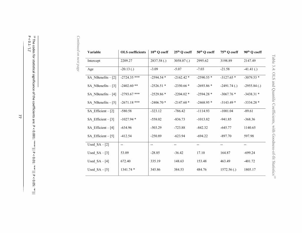
77

Table 3.4: OLS and Q

uantile Coefficients, with G

oodness-of-fit Statistics 19

90th Q coeff

2147.49

-41.41 (.)

-3079.53 *

-2955.84 (.)

-3438.31 *

-3334.28 *

-89.61

-368.36

1140.65

597.98

--

-699.24

-401.72

1805.17

75th Q coeff

3198.89

-21.58

-3127.65 *

-2491.74 (.)

-3067.76 *

-3143.49 *

-1001.04

-941.85

-645.77

-897.70

--

164.87

463.49

1572.56 (.)

50th Q coeff

2995.62

-7.03

-2590.55 *

-2693.86 *

-2594.28 *

-2468.95 *

-1114.93

-1013.82

-842.32

-694.22

--

17.10

153.48

484.76

25th Q coeff

3058.07 (.)

-5.07

-2162.42 *

-2350.66 *

-2204.02 *

-2147.60 *

-786.42

-836.73

-723.88

-623.94

--

-36.42

148.63

384.53

10th Q coeff

2837.58 (.)

-3.09

-2594.54 *

-2526.51 *

-2529.86 *

-2406.70 *

-323.12

-558.02

-503.29

-250.89

--

-28.85

335.19

345.86

OLS coefficients

2209.27

-20.13 (.)

-2724.35 ***

-2402.60 **

-2793.67 ***

-2671.18 ***

-580.58

-1027.94 *

-634.96

-412.54

--

53.09

672.40

1341.74 *

Variable

Intercept

Age

SA_NBenefits – [2]

SA_NBenefits – [3]

SA_NBenefits – [4]

SA_NBenefits – [5]

SA_Efficient – [2]

SA_Efficient – [3]

SA_Efficient – [4]

SA_Efficient – [5]

Used_SA – [2]

Used_SA – [3]

Used_SA – [4]

Used_SA – [5]

Continued on next page

19 The codes for statistical significance of the coefficients are: P < 0.001: ‘***’|| P < 0.01: ‘**’|| P < 0.05: ‘*’|| P < 0.1: ‘(.)’

78

Table 3.4 (Continued)

90th Q coeff

7351.63 *

4030.03 (.)

3524.45

4544.94 *

1787.64

1410.12

219.94

129.43

-45.29

759.10

444.33

45.73

0.454

2.609.456

75th Q coeff

2909.01

2344.99

2036.38

2353.88

980.66

-299.72

-463.80

-599.14

17.96

185.64

345.69

1160.49

0.364

2.532.723

50th Q coeff

1879.83

1186.21

1179.12

1326.43

440.20

-81.78

-212.65

-153.37

69.75

43.24

11.16

1425.85 (.)

0.278

2.456.699

25th Q coeff

570.39

130.39

44.80

105.48

-106.56

168.53

57.64

-50.38

141.25

61.82

30.49

1520.80 **

0.227

2.397.410

10th Q coeff

219.13

146.10

109.80

98.30

-278.91

-237.32

-355.21

-358.15

335.76

332.36

307.33

1378.07 **

0.194

2.371.533

OLS coefficients

2772.37 **

1597.12 (.)

1352.10

1645.38 (.)

564.86

539.20

-120.42

-293.21

492.11

603.31

1015.83 *

1929.46 **

0.333

2.529.573

Variable

Buy_wSubsidies – [2]

Buy_wSubsidies – [3]

Buy_wSubsidies – [4]

Buy_wSubsidies – [5]

Buy_wRemote – [2]

Buy_wRemote – [3]

Buy_wRemote – [4]

Buy_wRemote – [5]

Behavior – [2]

Behavior – [3]

Behavior – [4]

Behavior – [5]

Adjusted/Pseudo R2

AIC Values

79

Figures 3.3-3.5 show how the coefficients of three different predictors (SA_NBenefits, Buy_wSubsidies, Behavior) vary across their quantiles. Each figure has four images, one for each dummy value of the variable. Thus for instance, Figure 3.3[a] shows how the quantile coefficients of response vary specifically for those respondents who somewhat disagreed with the statement, ‘The use of smart appliances did not seem to benefit me,’ while Figure 3.3[b] shows the coefficients for respondents who were neutral to the same statement. In these figures, the y-axis shows the value of the coefficient, while the x-axis shows the quantile. The horizontal red lines denote the OLS coefficients, which are of course constant across quantiles. The black lines indicate the quantile coefficients, and these are dotted at the quantiles we measured, the 10th, 25th, 50th, 75th, and 90th. The figures are meant to visually highlight the divergences in the quantile coefficients from their OLS counterparts, and rely on the estimates in Table 3.4.

Figure 3.3[a-d]: Plotted OLS and QR Coefficients for Perceived Smart Appliance Benefits (SA_NBenefits) by Quantile

[a] Category 2 [b] Category 3

[c] Category 4 [d] Category 5

The statement ‘The use of smart appliances did not seem to benefit me’ has large and negative coefficients in each category and quantile, meaning that responsiveness was negatively related to this statement. The coefficients increase from the 10th to the 25th quantile, but then become more negative in general – they typically start higher than the OLS coefficients but end up lower among the more responsive participants. The higher categories (categories 4 and 5) are less negative at lower quantiles and more negative at higher quantiles, which possibly indicates a greater variation in flexibility at these levels.

Quantile

Coef

f. V

alue

Quantile

Coe

ff. V

alue

Quantile Quantile

80

Figure 3.4[a-d]: Plotted OLS and QR Coefficients for Role of Subsidies (Buy_wSubsidies) by Quantile

[a] Category 2 [b] Category 3

[c] Category 4 [d] Category 5

The question ‘Would subsidies play a role in deciding to buy smart appliances or an energy management system?’ has more respondents in the higher response categories. In general, these higher response categories have lower coefficients than the lower response categories. Additionally, the coefficients increase substantially from the lower to the higher quantiles, and are consistently different from the OLS coefficients. Figure 3.5[a-d]: Plotted OLS and QR Coefficients for Perceived Behavior Change (Behavior) by

Quantile [a] Category 2 [b] Category 3

[c] Category 4 [d] Category 5

The bulk of responses to the statement ‘Our behavior changed as the field test progressed’ fall in the middle three categories. While the coefficients of these three categories are similar at the 10th

Coe

ff. V

alue

Co

eff.

Val

ue

Coef

f. V

alue

C

oeff

. Val

ue

Quantile Quantile

Quantile Quantile

Quantile Quantile

Quantile Quantile

81

quantile, only those for category 2 (“No”) fall consistently as the quantiles increase, becoming negative at the 90th quantile. For the 3rd and 4th categories (“Neutral” and “Yes”), the coefficients fall until the median mark and then rise. In general though, they stay below the OLS coefficients, suggesting that outliers may have significantly influenced the OLS model in this case. 3.5 Discussion The Linear trial was set up in a way that roughly approximated the recommendations from existing literature on DR design: it used appropriate appliances – such as washing machines and dishwashers – a key component of successful DR [18]; it provided enabling technologies such as smart meters and tablets [19]; and it enrolled participants using an opt-in approach, which leads to higher average responses than opt-out approaches, even though participation rates are typically lower [26]. Given this, the results broadly show that maximizing the response to residential DR programs would indeed require inducing changes in behavior – in different ways – among different households. These changes in behavior are closely linked with user perceptions of the benefits of smart appliances, and with considerations of convenience and cost. Further, age will be likely to affect flexibility and response and must thus be factored in as well. The results of both the OLS and the quantile regressions – for those predictor variables which had significant coefficients – are discussed in greater detail listwise below. 3.5.1 Age In the OLS analysis, age has a negative coefficient, suggesting that in general, younger respondents are more likely to offer greater flexibility. This is in line with existing literature – such as Hauk et al.’s meta-analysis [42] – that states that younger populations tend to be more flexible in general and more comfortable with new technologies. Ota et al. [43] find that older populations have a lower electricity demand overall, which may also reduce their potential for flexibility. Yang et al. [44] use survey data from China to find that younger consumers are more likely to shift to ToU pricing programs than older ones. This result is further interpreted by the quantile analysis, which shows that respondent age doesn’t greatly affect response among the least flexible participants, but that there is a large negative relationship between age and flexibility among the highest quantiles. That is, age may not be a great predictor of inflexibility, but being younger does substantially increase response even among the most flexible respondents. For instance, among the least flexible 10% of users, an increase in age of one year saw a reduction of only 3 hours in total flexibility across the trial, but among the most flexible 10%, an increase in age of one year saw a reduction of 41 hours in total flexibility. This layering suggests that other concerns play a more significant role among the least responsive, rather than their age, and that a lack of response may therefore not be a function of such demographic variables.

82

3.5.2 Perceived Benefits from Using Smart Appliances Across the sample, participants were much less likely to offer flexibility if they perceived less of a benefit to using smart appliances. This extends existing findings [14,16], by demonstrating that not only do households want to better understand the potential benefits of DR, but that a DR program’s success hinges on this understanding. It also complements literature [19] on the actual enabling role of supporting technologies. Looking deeper, we see that at higher quantiles, the coefficients became more negative; i.e. among the participants who offered the greatest flexibility, a negative perception of the benefits of smart appliances tended to reduce flexibility much more than among those that offered the least flexibility. This result suggests that negative perceptions of the benefits of smart appliances are a big challenge, particularly among those who are otherwise likely to be more responsive to DR. However, it again suggests that population segments that are less likely to be responsive are less influenced by the perceived benefits of smart appliances, and may have other concerns that limit their response. 3.5.3 Usage of Smart Appliances Most people claimed to have used their smart appliances at least to some extent, and a greater extent of use was, expectedly, correlated with offering higher flexibility. This corroborates findings from comparable trials, where households that regularly used the smart appliances were more likely to have shifted their electricity usage [45]. Although less clear among the top and bottom deciles of the respondents, the general trend of flexibility being correlated with extent of smart appliance usage was consistent, and the correlation was uniformly stronger at higher quantiles of flexibility. 3.5.4 The Role of Subsidies in Deciding to Buy Smart Appliances Most respondents generally agreed that subsidies would indeed influence their decision to buy smart appliances. This aligns with the findings by Brent at al. [19] and Kessels et al. [21] about the role that financial savings can play on DR implementation. Respondents who were more influenced by subsidies were also less likely to offer flexibility in general, although the coefficients in the highest quantile of response deviated from this trend. Overall, it can be seen that the coefficients expectedly increase at higher quantiles. Thus among the least responsive participants, financial considerations were more inversely related with flexibility than among the most responsive. This suggests that – across the factors explored in this paper – price sensitivity is the main concern among less responsive populations.

83

3.5.5 Behavior Changes over the Course of the Field Test Respondents did not completely agree that their behavior had changed over the course of the field test, even though most of them had used their smart appliances. There was however a positive relationship between stated behavior change and actual flexibility. Among respondents who claimed that their behavior hadn’t changed, greater flexibility (i.e. at higher quantiles) was associated with decreasing coefficients, suggesting that they were less likely to have been among the most flexible. Among respondents who were neutral to somewhat agreeable on the behavior change, the flexibility tended to decrease towards the middle quantiles and increase rapidly towards the higher quantiles, suggesting that perhaps responses in those categories primarily populated the highest quantiles. These findings from the Linear DR trial cannot be directly compared with other trials, because most other trials have not combined DR demonstrations with a study of participant attitudes and behaviors. Further, we would exercise caution in generalizing the findings without additional future research, since the Linear trial was conducted with an unrepresentative sample and infeasible incentives, typical of many trials. Overall, however, our results strengthen and complement many of the general findings from existing literature, particularly via the OLS model. The quantile regression analysis further demonstrates that these findings are not uniformly applicable even within a limited sample, but are more nuanced, something that previous studies have not done. It reveals additional insights over the OLS model – and over existing literature – and demonstrates the variations in the determinants of flexibility, by showing that response is more affected (1) at the higher percentiles by factors such as age and perceived smart appliance benefits, and (2) at the lower percentiles by factors such as the availability of subsidies. The remaining factors from the surveys – such as the adequacy of consumption information, the impacts on convenience, and privacy – were not found to be significant, which is not in line with much existing literature [14,15,16,17]. This is possibly because of the considered design of the trial, or because the sample consisted of higher-income, pro-environment, early adopters of technology who opted to participate in it. The results however suggest that different strategies and incentives should be devised, customized to different population segments, in order to maximize the likelihood of success of future demand response programs. 3.6 Conclusions and Policy Implications The European interconnected market needs 3 GW in the primary reserves it uses to avoid grid instability. At a national level, Belgium further needs 500-600 MW in its strategic reserve. Demand response can thus play a large role in promoting national and regional energy security, aside from helping with the grid integration of renewables.

84

Studies on demand response have thus far focused on regulatory updates, consumer access, balancing markets, and wholesale markets. But a key challenge for DR is increasing consumer trust and participation [46]. The Clean Energy package of 2016 does propose access to smart meters and better information, and Belgium in particular is rolling out smart meters nationwide in a phased manner, starting with prosumers. However, no concrete steps have yet been outlined – at the European Union (EU) or national levels – on how to increase consumer uptake of DR. This paper analyzes a concluded Belgian residential electricity demand response trial, using response data from 155 participating families, coupled with accompanying surveys that were used to gauge these families’ attitudes to smart appliances. The objective of combining the two was to understand in detail how demand flexibility is correlated with users’ perceptions of and concerns with smart appliances, and to thereby offer specific recommendations to promote consumer participation in DR. The paper relies on the method of quantile regression analysis to dissect user responses and see how these perceptions and concerns vary at different levels of response. The results showed that there is a clear link between modest changes in user behavior and the demand flexibility that can be realized. Thus, for future DR programs to be successful, policymakers should target small shifts in behavior – avoiding the excess changes that might result in user inconvenience – and incorporate these effects into conventional estimates of the economic feasibility of such programs. Flexibility was also found to be linked to user perceptions of the benefits of smart appliances. It is particularly important that groups that are more likely to be responsive should perceive smart appliances as being beneficial. Thus, in order to induce the aforementioned behavioral changes, DR implementation should be enabled by fully functional technologies and could accompanied by awareness campaigns among such groups on the benefits of smart appliances. Respondents were found to be sensitive to an availability of subsidies for the smart appliances, particularly among less flexible groups, suggesting that either they may perceive such appliances as being too expensive or they may be more sensitive to prices. Uptake of such DR programs among less flexible groups may thus be maximized by offering financial incentives, or by explaining the potential for such programs to lead to financial benefits for the users. Lastly, age was found to have an inverse relationship with the potential for demand flexibility among more responsive groups, possibly because younger participants were more comfortable with technology, more aware of environmental issues, or more likely to have a smaller family. Thus, while younger respondents may represent low-hanging fruit to realize some of the benefits of DR, in the longer term, more effort should be invested into getting older segments involved in such programs. Among less responsive groups, age was not as significant of a factor, suggesting that these segments may have other concerns that might be better addressed by the steps outlined above. In this way, the overall analysis complemented findings from existing research and then uncovered some of the complexities hidden in these general findings. However, the results in this paper are drawn from a limited sample of 155 families in Flanders, Belgium. Further, the Linear trial project was not representative, nor was it designed in a way that could be feasible for a broader rollout.

85

Lastly, we note that respondent attitudes may have been influenced by their engagement in the trial, while their response may in turn have been influenced by their changing attitudes, in a form of a bi-directional causality. Future research should look at a broader and more representative sample20 with greater focus on how to build customer engagement and reduce resistance to participating in DR, by looking at the concerns of each segment of the target population. For now, Denmark and Germany are leading on projects focusing on consumer engagement in Europe [46]. In the US, consumer behavior studies are examining customer participation in DR, and the influence of enabling technologies on customer response [47,48]. Building on this current study, a deeper look into the relationships between customer response and perceptions, in a broader range of regions, would greatly help with the implementation of the EU Clean Energy package and the ensured security of energy supply.

20 Keeping in mind however that rollouts often proceed in a phased manner, with an initial focus on early adopters such as those who participated in the Linear project

86

Appendix 3-A: Predictor Variables The 40 predictor variables that were used in the analysis – and were drawn mainly from the surveys – are listed in Table 3-A.1 below.

Table 3-A.1: Predictor Variables Question Variable Type Gender Nominal Age Continuous During the field test, Linear showed variable rates. To what extent did you take these rates into account when using the devices?

Ordinal

Were there certain household routines or habits that restricted flexibility? Nominal During Linear you had a tablet available. Was the information you received through the tablet about your energy consumption sufficient?

Nominal

Was the information from the device/controller displays sufficient? Nominal How frequently did you check your smart meter? Ordinal Is the following information easy to read from the smart meter display? - Current consumption

Nominal

Is the following information easy to read from the smart meter display? - Rate type Nominal

Do you believe that you consumed less thanks to this smart meter in your home? Nominal

Were you worried when using your appliances about your privacy? Ordinal Did you experience a loss in comfort by participating in Linear? Ordinal To what extent do you agree with the following statements: Our behavior changed as the field test progressed

Ordinal

To what extent do you agree with the following statements I would have liked more information about when the flexibility that I give is used

Ordinal

To what extent do you agree with the following statements: The use of smart appliances seems to have no benefits

Ordinal

To what extent do you agree with the following statements: Smart appliances are easy to work with

Ordinal

To what extent do you agree with the following statements: The use of smart appliances makes me work more efficiently

Ordinal

To what extent do you agree with the following statements: I use the various features of smart appliances

Ordinal

Continued on next page

87

Table 3-A.1 (Continued) Question Variable Type

To what extent do you agree with the following statements: I made use of my smart appliances

Ordinal

To what extent do you agree with the following statements: I questioned the safety of smart appliances (eg risk of fire)

Ordinal

To what extent do you agree with the following statements: I think smart appliances allow too little control to the user

Ordinal

To what extent do you agree with the following statements: I doubt these smart appliances will be more environmentally friendly

Ordinal

What factors might play a role in deciding to buy smart appliances or an energy management system? - Environmental considerations

Ordinal

What factors might play a role in deciding to buy smart appliances or an energy management system? - Savings (€)

Ordinal

What factors might play a role in deciding to buy smart appliances or an energy management system? - Subsidies

Ordinal

What factors might play a role in deciding to buy smart appliances or an energy management system? - Ability to operate appliances remotely

Ordinal

What factors might play a role in deciding to buy smart appliances or an energy management system? - Experimenting with new technology

Ordinal

What factors might play a role in deciding to buy smart appliances or an energy management system? - Greater stability of energy supply

Ordinal

Pre-trial scores on Safety Ordinal Pre-trial scores on Comfort Ordinal Pre-trial scores on Control Ordinal Pre-trial scores on Cost Ordinal Pre-trial scores on Privacy Ordinal I can generally work with high-tech products Ordinal New technology is often too complex to be useful Ordinal Technology gives people more control over their daily lives Ordinal Technology makes me more efficient in my work Ordinal Changes to mean scores on attitude Ordinal Total installed PV power (kWh) Continuous

Mean scores on Perceived environment friendliness Ordinal

88

Appendix 3-B: Diagnostics for Model OLS Regression Diagnostic plots for the OLS regression, for the model captured in Equation 5, are provided in Figure 3-B.1 below.

Figure 3-B.1[a-d]: OLS Diagnostic Plots

These plots show that the residuals decrease as the fitted values increase, that the data is right-skewed, and that the variance might not be equal, although there are no influential cases that fall outside of Cook’s distance lines. Overall, the data is not normally distributed or homoscedastic. Chi-squared tests of correlations among the categorical variables summarized in Table 3.2 show correlations between questions 2 (SA_NBenefits) and 4 (Used_SA), and between questions 3 (SA_Efficient) and 4 (Used_SA). However, a check for multicollinearity among the variables in Table 3.2 yields the generalized variance inflation factors (GVIFs) outlined in Table 3-B.1 below. The low values indicate that collinearity is within acceptable limits in this model.

Table 3-B.1: Test for Multicollinearity Ques GVIF Df GVIF^(1/(2*Df)) 1 1.379 1 1.174 2 2.340 4 1.112 3 2.773 4 1.136 4 2.614 3 1.173 5 2.034 4 1.092 6 1.721 4 1.070 7 1.970 4 1.088

89

References [1] US Environmental Protection Agency. (2018). Inventory of US greenhouse gas emissions and sinks, 1990-2016. EPA. https://www.epa.gov/sites/production/files/2018-01/documents/2018_complete_report.pdf [2] Elia. (2008) The primary reserve: A solution for stabilizing the frequency in the European interconnected system. Elia. http://www.elia.be/~/media/files/Elia/Products-and-services/ProductSheets/S-Ondersteuning-net/S1_F_RES_PRIMAIRE.pdf [3] Elia. Ancillary services, http://www.elia.be/en/products-and-services/ancillary-services [accessed 03.07.2018] [4] Restore. Belgian TSO Elia in demand response first, https://restore.energy/export/pdfNews/113 [accessed 05.08.2018] [5] World Energy Council. (2016). E-storage: Shifting from cost to value - Wind and solar applications. World Energy Council. https://www.worldenergy.org/wp-content/uploads/2016/03/Resources-E-storage-report-2016.02.04.pdf [6] Eurelectric. (2017). Dynamic pricing in electricity supply. Eurelectric. http://www.elecpor.pt/pdf/16_02_2017_Dynamic_pricing_in_electricity_supply.pdf [7] Gils, H.C. (2014). Assessment of the theoretical demand response potentnial in Europe. Energy, 67, 1-18. https://doi.org/10.1016/j.energy.2014.02.019 [8] European Commission. Commission proposes new rules for consumer centered clean energy transition, https://ec.europa.eu/energy/en/news/commission-proposes-new-rules-consumer-centred-clean-energy-transition [accessed 28.04.2018] [9] Joint Research Center. Smart Grid Projects Map, http://ses.jrc.ec.europa.eu/sites/ses.jrc.ec.europa.eu/files/u24/2014/project_maps_28_april_2014.html [accessed 18.03.2018] [10] US Department of Energy. Smart Grid Demonstration Program, https://www.smartgrid.gov/recovery_act/overview/smart_grid_demonstration_program.html [accessed 18.03.2018] [11] SEDC. (2017). Explicit demand response in Europe – Mapping the markets 2017. SEDC. http://www.smartenergydemand.eu/wp-content/uploads/2017/04/SEDC-Explicit-Demand-Response-in-Europe-Mapping-the-Markets-2017.pdf [12] Gyamfi, S., Krumdieck, S., & Urmee, T. (2013). Residential peak electricity demand response - Highlights of some behavioural issues. Renewable and Sustainable Energy Reviews, 25, 71–77. https://doi.org/10.1016/j.rser.2013.04.006 [13] Bartusch, C., Wallin, F., Odlare, M., Vassileva, I., & Wester, L. (2011). Introducing a demand-based electricity distribution tariff in the residential sector: Demand response and customer perception. Energy Policy, 39(9), 5008–5025. https://doi.org/10.1016/j.enpol.2011.06.013

90

[14] Hall, N. L., Jeanneret, T. D., & Rai, A. (2016). Cost-reflective electricity pricing: Consumer preferences and perceptions. Energy Policy, 95, 62–72. https://doi.org/10.1016/j.enpol.2016.04.042 [15] Muratori, M., Schuelke-Leech, B. A., & Rizzoni, G. (2014). Role of residential demand response in modern electricity markets. Renewable and Sustainable Energy Reviews, 33, 546–553. https://doi.org/10.1016/j.rser.2014.02.027 [16] Darby, S. J., & McKenna, E. (2012). Social implications of residential demand response in cool temperate climates. Energy Policy, 49, 759–769. https://doi.org/10.1016/j.enpol.2012.07.026 [17] Parag, Y., & Butbul, G. (2018). Flexiwatts and seamless technology: Public perceptions of demand flexibility through smart home technology. Energy Research and Social Science, 39, 177–191. https://doi.org/10.1016/j.erss.2017.10.012 [18] Mert, W. (2008). Consumer acceptance of smart appliances. European Commission. https://ec.europa.eu/energy/intelligent/projects/sites/iee-projects/files/projects/documents/e-track_ii_consumer_acceptance.pdf [19] Brent, D. A., Friesen, L., Gangadharan, L., & Leibbrandt, A. (2016). Behavioral insights from field experiments in environmental economics. Monash Business School, discussion paper 34/16. https://www.monash.edu/__data/assets/pdf_file/0009/926199/3416behavioralbrentfriesengangadharanliebbrandt.pdf [20] US Department of Energy. Consumer behavior studies, https://www.smartgrid.gov/recovery_act/overview/consumer_behavior_studies.html [accessed 27.07.2018] [21] Kessels, K., Kraan, C., Karg, L., Maggiore, S., Valkering, P., & Laes, E. (2016). Fostering Residential Demand Response through Dynamic Pricing Schemes: A Behavioural Review of Smart Grid Pilots in Europe. Sustainability, 8(9), 929. http://www.mdpi.com/2071-1050/8/9/929 [22] Vesterberg, M. (2016). The hourly income elasticity of electricity. Energy Economics, 59, 188–197. https://doi.org/10.1016/j.eneco.2016.08.014 [23] Silva, S., Soares, I., & Pinho, C. (2017). Electricity demand response to price changes: The Portuguese case taking into account income differences. Energy Economics, 65, 335–342. https://doi.org/10.1016/j.eneco.2017.05.018 [24] Irish Commission for Energy Regulation. (2011). Electricity smart metering customer behavior trials findings report. CER. https://www.cru.ie/wp-content/uploads/2011/07/cer11080ai.pdf [25] Cosmo, V. Di, & O’Hora, D. (2017). Nudging electricity consumption using TOU pricing and feedback: evidence from Irish households. Journal of Economic Psychology, 61, 1–14. https://doi.org/10.1016/j.joep.2017.03.005 [26] Parrish, B., Gross, R., & Heptonstall, P. (2019). On demand: Can demand response live up to expectations in managing electricity systems? Energy Research and Social Science, 51, 107-118. https://doi.org/10.1016/j.erss.2018.11.018

91

[27] Srivastava, A., Van Passel, S., & Laes, E. (2018). Assessing the success of electricity demand response programs: A meta-analysis. Energy Research and Social Science, 40, 110-117. https://doi.org/10.1016/j.erss.2017.12.005 [28] Bertoldi, P., Zancanella, P., and Boza-Kiss, B. (2016). Demand response status in EU Member States. JRC Science for Policy. http://publications.jrc.ec.europa.eu/repository/bitstream/JRC101191/ldna27998enn.pdf [29] Elia. Adequacy study for Belgium: The need for strategic reserve for winter 2018-19, http://www.elia.be/en/about-elia/newsroom/news/2017/20171130_Strategic-reserve-for-winter-2018-19 [accessed 07.06.2018] [30] Linear. Home page, www.linear-smartgrid.be [accessed 15.07.2018] [31] Kaza, N. (2010). Understanding the spectrum of residential energy consumption: A quantile regression approach. Energy Policy, 38(11), 6574–6585. https://doi.org/10.1016/j.enpol.2010.06.028 [32] Khanna, N. Z., Guo, J., & Zheng, X. (2016). Effects of demand side management on Chinese household electricity consumption: Empirical findings from Chinese household survey. Energy Policy, 95, 113–125. https://doi.org/10.1016/j.enpol.2016.04.049 [33] Romero-Jordán, D., del Río, P., & Peñasco, C. (2016). An analysis of the welfare and distributive implications of factors influencing household electricity consumption. Energy Policy, 88, 361–370. https://doi.org/10.1016/j.enpol.2015.09.037 [34] The Linear Consortium. (2014). Linear: The report. Linear. http://www.linear-smartgrid.be/sites/default/files/boekje_linear_okt_2014_boekje_web.pdf [35] Statbel. An overview of Belgian wages and salaries, https://statbel.fgov.be/en/themes/work-training/overview-belgian-wages-and-salaries [accessed 20.08.2018] [36] Broman Toft, M., Schuitema, G., & Thøgersen, J. (2014). Responsible technology acceptance: Model development and application to consumer acceptance of Smart Grid technology. Applied Energy, 134, 392–400. https://doi.org/10.1016/j.apenergy.2014.08.048 [37] Hao, L; Naiman, D. (2007). Quantile Regresssion. Quantile Regression, 1–6. https://doi.org/10.1002/9780470057339.vnn091 [38] Takeuchi, I., Le, Q. V., Sears, T., & Smola, A. J. (2005). Nonparametric Quantile Regression. Journal of Machine Learning Research, 7, 1001–1032. https://doi.org/10.1080/10485259508832642 [39] Feise, R. J. (2002). Do multiple outcome measures require p-value adjustment? BMC Medical Research Methodology. https://www.ncbi.nlm.nih.gov/pmc/articles/PMC117123/ [40] Koenker, R. (1981). A note on studentizing a test for heteroscedasticity. Journal of Econometrics, 17(1), 107-112. https://doi.org/10.1016/0304-4076(81)90062-2 [41] Koenker, R., & Machado, J. A. F. (1999). Goodness of Fit and Related Inference Processes for Quantile Regression. Journal of the American Statistical Association, 94(448), 1296–1310. https://doi.org/10.1080/01621459.1999.10473882

92

[42] Hauk, N., Hüffmeier, J., & Krumm, S. (2018). Ready to be a Silver Surfer? A Meta-analysis on the Relationship Between Chronological Age and Technology Acceptance. Computers in Human Behavior, 84, 304–319. https://doi.org/10.1016/j.chb.2018.01.020 [43] Ota, T., Kakinaka, M., & Kotani, K. (2018). Demographic effects on residential electricity and city gas consumption in the aging society of Japan. Energy Policy. https://doi.org/10.1016/j.enpol.2018.01.016 [44] Yang, Y., Wang, M., Liu, Y., & Zhang, L. (2018). Peak-off-peak load shifting: Are public willing to accept the peak and off-peak time of use electricity price? Journal of Cleaner Production. https://doi.org/10.1016/j.jclepro.2018.06.181 [45] Kobus, C. B. A., Klaassen, E. A. M., Mugge, R., & Schoormans, J. P. L. (2015). A real-life assessment on the effect of smart appliances for shifting households’ electricity demand. Applied Energy, 147, 335–343. https://doi.org/10.1016/j.apenergy.2015.01.073 [46] Giordano, V., Meletiou, A., Covrig, C.F., Mengolini, A., Ardelean, M., Fulli, G., Jimenez, M.S., and Filiou, C. (2013). Smart grid projects in Europe: Lessons learned and current developments. JRC Science and Policy. https://ses.jrc.ec.europa.eu/sites/ses.jrc.ec.europa.eu/files/publications/ld-na-25815-en-n_final_online_version_april_15_smart_grid_projects_in_europe_-_lessons_learned_and_current_developments_-2012_update.pdf [47] US Department of Energy. Demand response – policy, https://www.energy.gov/oe/services/electricity-policy-coordination-and-implementation/state-and-regional-policy-assistanc-4 [accessed 18.08.18] [48] US Department of Energy. (2015). Interim report on customer acceptance, retention, and response to time-based rates from the consumer behavior studies. US Department of Energy. https://www.energy.gov/sites/prod/files/2015/06/f24/ARRA-CBS_interim_program_impact_report_June2015.pdf

93

Estimating Acceptability: Load Controls in a Developed Country 4. Chapter based upon: Srivastava, A., Van Passel, S., Kessels, R., Valkering, P., & Laes, E. Reducing winter peaks in electricity consumption: A choice experiment to structure demand response programs. Working paper 4.1 Introduction The electricity sector generates up to 30% of global greenhouse gas emissions [1]. At the same time, increasing electricity consumption – coupled with an ageing grid infrastructure – presents a challenge for energy security. To manage this, the European electricity market needs 3 gigawatts (GW) in its primary operating reserve alone21 [2]. Demand response (DR) programs are a potential avenue to aid with the grid integration of renewables, and with improving energy security [2,3]. The European Commission (EC) estimates a total response potential of 160 GW by 2030, with around 40% of this potential for flexibility coming from the residential sector [4], although achievable potential is likely lower [5]. DR is thus being promoted through enabling policy frameworks and trial programs in many European countries, particularly in the residential sector [6]. However, the introduction of DR in the residential sector has had mixed results. Some studies have found their implementation to be successful. For instance, Bartusch et al. [7] found through an analysis of a time-of-use (ToU) pricing pilot and accompanying interviews that households in Sweden do indeed act on intrinsic price signals by decreasing demand in peak periods and shifting electricity use to off-peak periods. Faruqui and Sergici’s synthesis of 15 heterogenous DR trials and implementations in the US and Canada [8], and a UK government review of 30 varied DR trials in various countries [9], also found that households do respond to price changes, although the magnitude of response depends on several factors. However, on other occasions, varying consumer attitudes have limited the responsiveness to such programs [10]. For instance, consumers were found to be less price-sensitive when they were more concerned about minimizing their inconvenience and discomfort, or about privacy and safety [11,12,13]. Hall et al. [14] identified – using a random sample of respondents with higher rates of employment than the population average – that households are open to ToU pricing but want more information to understand the potential benefits of DR. Similarly, Brent et al. [15] reviewed a number of field experiments in dynamic pricing and stated that knowledge about consumption can maximize the effectiveness of time-varying pricing, and that the availability of enabling technology increases the effectiveness of such pricing. Still other studies have offered conflicting findings, which suggest that household preferences are not homogenous and can depend on the structure of the DR program. For instance, the Irish energy

21 An operating reserve is the spare generating capacity available to meet demand in case of a sudden need. Specifically, the European primary reserve is meant for frequency stabilization in the event of grid imbalances

94

regulator [16] found through a smart metering trial among a representative sample of 5000 households that ToU tariffs reduced electricity usage, and that higher-consuming households delivered greater reductions. However, Gyamfi et al. [10] reviewed pricing-based DR literature and stated that a high number of households – particularly the richer ones – did not actually respond to price signals. Further, Srivastava et al. [17] found through a meta-analysis of 32 DR initiatives that success in DR was also related to the socio-economic contexts around their implementation. There is an increasing focus in research on understanding context-specific consumer preferences and behaviors, and determining how they affect response to DR programs [18]. Existing research into DR programs has however made limited use of stated preference approaches. Ericson [19] estimated a discrete choice model – using existing opt-in data from a critical peak pricing (CPP) experiment in Norway – to understand the bases on which consumers choose between tariffs. Buryk et al. [20] used a web-based labelled discrete choice experiment (DCE) using convenience sampling – varying only the price attribute – to determine whether disclosing the environmental and system benefits of dynamic tariffs could increase customer adoption. Pepermans [21] used a DCE with snowball sampling to assess the extent to which consumers in Flanders, Belgium would use smart meters as an enabling technology, although the design did not include dynamic pricing schemes and did not consider the likely correlations between cost savings and impacts on comfort. Other studies [22,23,24,25] have used choice experiments to understand preferences for other aspects of electricity generation and provision. Current choice modeling research has not focused however on the actual structuring of DR programs; such an approach would allow the estimation of a monetary value of the different attributes of DR programs, thereby helping better structure such programs in the future. 4.1.1 Opportunity for Demand Response in Belgium There is an interest in Belgium in implementing DR in the residential sector, and the national transmission system operator is exploring ways to reward flexible consumers with lower energy bills [26]. Such flexibility is particularly important during the winter months, in the short term, for two reasons. The first is on the demand side: Electricity demand typically peaks in the winter months, reaching up to 14,000 megawatts (MW), and is about 2000 MW higher than in the summer [27]22. On the supply side, Belgium has been largely reliant upon nuclear power plants (NPPs) – Figure 4.1 shows the country’s generation mix – which are old and unreliable; between 2010 and 2014, electricity generation fell by 24%, primarily because of extensive outages at its NPPs [27], although it has since recovered.

22 The residential sector comprised about 23.1% of total consumption [27]

95

Figure 4.1: Shares of Electricity Generation in Belgium in 2014

Source: International Energy Agency [27]

Although Belgium will phase out its NPPs over the medium to long term [28,29], there is a short- to medium-term risk to the security of supply due to the possibility of further outages, particularly during the winter months. Reducing winter peaks in demand would reduce the need for costly peaking generation and would also help manage the markets in case of such outages. 4.1.2 Scope of Paper This paper uses a stated preference approach to estimate a monetary value, to consumers, of different attributes of DR programs. It conducts a DCE in the Belgian region of Flanders to gauge respondents’ willingness to enroll in a winter DR program in return for a monetary compensation. In this way, the paper examines consumer preferences for electricity contracts in the Belgian context. To our knowledge, previous attempts to structure DR programs have not taken consumer preferences into account, and choice experiments have not been used to study consumers’ willingness to shift electricity consumption. Thus, the paper fills critical gaps in research with an aim to aid in structuring a Belgian DR program that could reduce the winter peaks in electricity demand in the short- to medium-term. 4.2 Methods 4.2.1 Discrete Choice Experiments DCEs are widely used to study people’s preferences for certain attributes of products or services in different applied fields such as marketing, transport, health economics, and environmental economics. They are an attractive tool to value non-market attributes of goods and services or derive their non-consumptive values. They have not however been used in understanding preferences for DR programs.

NPPs47,20%

Natural Gas27,00%

Biofuels and Waste7,90%

Wind6,50%

Coal6,20%

Solar4,00%

Other1,20%

96

A DCE offers respondents several choice sets with a number of alternatives in each choice set, where each alternative is a combination of levels of different attributes. For each choice set, respondents indicate the alternative they like better. The most statistically efficient design is determined by means of the Bayesian D-optimality criterion [30]. Such a design guarantees that all parameters can be estimated with maximal precision. DCEs rely on the assumption that choices between alternative options reflect the utility that accrues from those alternatives, as derived from random utility theory [31]. This framework states that the utility Uj associated with an alternative j is the sum of its systematic and random components:

Uj = Vj + εj = xʹjβ + εj (1) where Vj is the indirect utility function of alternative j, xj is the vector describing the attribute levels of alternative j, β is the vector of preference parameters representing changes in utility arising from changes in the attribute levels, and εj is the stochastic error term. The basic model used to analyze choice data is McFadden’s [32] multinomial logit (MNL) model. Given a choice set with J alternatives, the probability that an individual i ϵ {1,…, N} in the sample chooses alternative k is defined as :

Pik(MNL) = exp (xʹikβ) / ΣJj=1 [ exp (xʹijβ)] (2)

The MNL model is restricted in that preferences are assumed to be homogenous across respondents. Therefore, current modeling practice has shifted toward the more flexible panel mixed logit (PML) model that accounts for heterogeneous preferences across respondents and correlation across repeated choices from the same respondent [33]. This model assumes a distribution of preference weights across the sample reflecting differences in preferences among respondents. This means that, unlike the MNL model, which estimates only the mean preference effect of an attribute level, the PML model yields both a mean effect and a subject standard deviation denoting the individual variation around it. Formally, the mixed logit probabilities are the integrals of standard logit probabilities over a density of random parameters as denoted by

Pik(PML) = ∫ Pik(MNL).f(β).dβ (3) where f(β) is a density function. To estimate the random parameters, we use the hierarchical Bayes (HB) technique in the JMP 14 platform – based on 10,000 iterations, with the last 5000 used for estimation – under the assumption of normally distributed preference parameters without correlation between attributes. These estimated random parameters model the unobserved heterogeneity in the respondents’ preferences. The marginal willingness to accept (WTA) a compensation for an attribute A, if utility is linear in the preference parameters, is measured as its preference weight divided by the marginal utility of money M, where the latter is the negative of the preference weight of the payment attribute. This is shown as :

97

WTPA = βA / (-βM) (4)

Lastly, for the policy simulations conducted in Section 4.3.3, which are based on the PML model estimates, we apply the approach used by Bennett et al. [34]. In these simulations, we estimate the predicted enrolment probability in a DR program k for respondent i in the sample by the binomial logit characterization:

Pik(Enroll) = exp (βxxk + βyyik) / [1 + exp (βxk)] (5) where βx is the vector of main-effect attribute parameters, βz is the vector of subject-effect parameters, and zik is the vector of user-specific variables. We then estimate the minimum payment ck for program k as the level of compensation at which the model predicts a targeted enrolment rate of R:

ΣNi=1 F [Pik(Enroll) | ck] / N = R (6)

where F [.] takes a value of 1 if Pik > 0.5, and 0 otherwise. For the policy simulations, we estimate ck for various values of R, i.e. we estimate the minimum payments necessary to predict various enrolment rates of sample households. 4.2.2 Background Literature and Consultations In Belgium, a DR field test in 2011 called Linear secured the participation of 240 families in the region of Flanders, 54 of whom were introduced to ToU pricing while the remaining 186 were provided with three smart appliances: washing machines, dishwashers, and tumble dryers23. The field test revealed that response to the ToU pricing was weak, while the response to the smart appliance program was higher – an extrapolation of the results to the Belgian context was shown as offering the potential to deliver up to 280 MW of flexibility through such appliances alone [35,36]. We drew on the results of this field test and chose to adopt a design based on smart appliances, rather than on time-based pricing of electricity. This decision also took into account that only a 30% share of the electricity tariff in Belgium is a variable component; imposing time-based pricing on this component would have a very limited impact on the overall tariff. For linguistic and cultural consistency, we focused our study on Flanders. We organized stakeholder consultations with sector experts, including representatives of the Flemish energy regulator (VREG) and the Flemish environment ministry (LNE), in designing the attributes and alternatives. Through these consultations, we validated that future DR programs would need to address the higher winter peaks in demand.

23 These smart appliances had a delayed start option – families were allowed to configure the start of their appliances at any time but with a maximum programmable delay of 24 hours, so long as they finished their cycles before the deadlines defined. The participants received a fee for the flexibility they offered

98

We focused on the same appliances that were used to deliver flexibility in the Linear field test – washing machines, dishwashers, and tumble dryers – for consistency. These three appliances are responsible for a considerable share (28%) of household electricity use [37]. We thus excluded the following categories of appliances: (i) other large appliance such as refrigerators, (ii) entertainment appliances such as televisions – we expected that respondents would be less flexible with these, (iii) standby and limited-use appliances such as coffee machines, (iv) heat pumps because of their low market penetration [38], and (v) heating systems since they are largely powered by natural gas, and not by electricity [39]. In the DR programs in the DCE, the selected appliances would have the ability to be externally controlled, using controllers installed on these appliances, for a few hours per day at most. We selected the numbers of hours in which to control loads based on the average electricity load curves for Belgium, which we sourced from the national transmission system operator [40]. For the compensation, we determined that the annual average household electricity bill in Flanders was approximately €1000 [41], implying that the average monthly bill would be in the range of €80-€85. We then aimed to offer respondents amounts in the range of 10-30% of an average monthly bill as total compensation across the annual duration of the program. 4.2.3 Pilot Choice Experiment Based on these inputs, we first conducted a pilot experiment consisting of 8 choice tasks, with each task offering two hypothetical DR programs. We created a Bayesian D-optimal design of 16 choice sets which we divided into two surveys of 8 choice sets. The design is Bayesian because it includes prior knowledge about the parameters – which improves the efficiency and accuracy of the design [42] – in the form of a parameter distribution in the design process24 [30]. We converted expected preference rankings of the attribute levels into prior mean values of our prior distribution, and allowed for a large amount of uncertainty around our expectations by specifying large prior variances. We then generated the designs in JMP 14. The structure and purpose of the DR program was explained to respondents before they were presented with the choice sets. Respondents who did not own a washing machine were not considered eligible for the DCE. Besides the two alternative programs, each choice set also included a ‘no-choice option’ allowing respondents to opt out from any of the presented programs and stay with their current consumption pattern. The pilot DCE questionnaire was circulated among author networks, and obtained 47 usable responses in total. The initial results – listed in Appendix 4-B – indicated that only the parameter

24 To some extent, the results depend on the prior information — one advantage of the Bayesian approach is that it allows the incorporation of this information, which is useful and necessary. It is nevertheless helpful for the interpretation of the results to disentangle the role of prior information. While studies could provide comparisons of prior and posterior distributions, these statistics are not necessarily very informative about the relative importance of the prior. They require repetitive re-runs of the model with randomly modified prior parameter values. Other formal approaches to prior sensitivity analysis are not commonly used due to their high computational costs [43]. Müller [44] proposes additional statistics to clarify the role of prior information, although these are not yet widely used

99

estimates for the number of hours per day that appliances would be controlled, and the compensation required, were statistically significant. Notably, the no-choice parameter was found to be significant in the pilot results, indicating either that respondents’ utilities increased by choosing not to choose, or that respondents did not find any of the choices of DR program particularly appealing. Across the choice sets presented, respondents chose the ‘no-choice’ option in 36.9% of the cases. 4.2.4 Main Choice Experiment The design of the main DCE was thus informed by (i) research into the Belgian electricity market, (ii) lessons from the Linear DR trial, (iii) stakeholder consultations with electricity sector experts, and (iv) results from a pilot DCE. Based on the response to the pilot, we modified the experiment in three ways: (i) the explanation of the choice task exercise in the questionnaire was improved and retained next to the choice sets for easy reference; (ii) the levels of the attributes were more clearly specified to improve understandability; and (iii) the presentation of the attributes was simplified. The attributes and levels used in the main experiment are laid out in Table 4.1, where the levels are listed in increasing order of their expected preference.

Table 4.1: Main DCE - Attributes and Levels Attribute Level 1 Level 2 Level 3 Hours of day that appliances would be controlled

07.00-09.00 and 18.00-20.00

17.00-20.00 18.00-20.00

Days of week that program would run

All 7 days All 5 weekdays Any 2 weekdays

Months of the year that program would run

1 October – 1 April 1 November – 1 March

1 January – 1 March

Appliances that would be controlled when program is running

Washing machine, dishwasher, tumble dryer

Washing machine and dishwasher

Washing machine only

Compensation required to participate

€10 €18 €25

As in the pilot phase, owning a washing machine was a minimum criterion to participate. For the attribute on ‘Appliances that would be controlled,’ in order to avoid splitting the sample based on appliance ownership, we asked the respondents to assume that they owned all three appliances. A last modification to the DCE was that we reduced the number of choice sets in the survey from 8 to 6, to reduce the risk of respondent fatigue, which could have partly contributed to the selection of the ‘no-choice’ options in the pilot testing. The structure and purpose of the DR program was again explained to respondents before they were presented with the choice sets. As in the pilot DCE, respondents were given the option to remain

100

with their current consumption structure. Accordingly, we generated a Bayesian D-optimal design of 12 choice sets that we divided into two surveys – a sample choice set is shown in Figure 4.2. In determining the prior parameter distribution, we drew on the parameter estimates from the analysis of the pilot data. The Bayesian designs were generated again in JMP 14.

Figure 4.2: Sample Choice Set Used in Main DCE

The choice experiment was accompanied by questions on appliance operation, as well as on respondents’ tariff structures and billing amounts. A separate section captured demographic information on age, gender, income, education, and dwelling characteristics. Additional questions were included to gauge respondents’ attitudes towards data privacy, environmental issues, and new technologies. All questions were phrased in neutral language to minimize respondent manipulation, and we attempted to reduce any potential hypothetical bias by explaining the real-life potential for such programs. In order to encourage respondents to fill out the survey, we offered to donate €0.50 to a charity of their choice upon their completion of the questionnaire. The full survey is listed in Appendix 4-A. To reach out to respondents, the questionnaire was disseminated online through Qualtrics. As it was conjectured that younger, well-educated households would be more accepting of smart appliances, we decided to aim at an oversampling of these segments25. We thus circulated the survey – adopting a mix of random and convenience sampling techniques – among (i) authors networks, (ii) different residential community groups in Flanders via Facebook, (iii) families that had participated in the Linear field test, (iv) university students, and (v) a Flemish organization working on sustainable technologies. The survey ran from July until early October 2018, and generated 186 usable responses in total. We do not have information about the non-response rates, because of the open nature of dissemination of the questionnaire. These responses were analyzed separately from the 47 responses in the pilot phase, owing to the modifications in the attributes and levels. All the data was anonymous and confidential.

25 Expert consultations corroborated that since typical DR rollouts proceed in a phased fashion, obtaining a sample that consists of early adopters who are more likely to embrace such a program would yield more valuable findings, rather than a broader sample that might yield less information

101

4.3 Results 4.3.1 Respondent Characteristics Descriptive statistics of the 186 respondents are listed in Table 4.2. As expected, the sample is younger and more educated than the overall population, although there is a slight underrepresentation of females.

Table 4.2: Respondent Characteristics Relative to Belgian population Characteristic Level Percentage Belgian Population

Age (Years) [1] 18-29 [2] 30-44 [3] 45-59 [4] 60 or more

47.3% 18.3% 21.5% 11.8%

15-24: 11.3% 25-54: 40.1% 55-64: 14.2%

65 or more: 18.6% Gender Male

Female 53.8% 44.1%

Male: 49.2% Female: 50.8%

Net Monthly Household Income

[1] <€2000 [2] €2000-€3000 [3] €3000-€4000 [4] €4000-€5000 [5] >€5000

8.6% 14.0% 14.5% 20.4% 14.5%

Per capita: €3445

Educational Degree Attained

[1] High school [2] Bachelor’s [3] Professional Bachelor’s [4] Master’s or higher

21.0% 17.2% 10.8% 48.9%

Upper secondary: 36%

Tertiary: 35%

Housing Type Apartment House

19.4% 79.6%

Apartments: 22% Houses: 77%

Number of People in Household

1-2 3-4 5-6

31.2% 53.2% 14.5%

Average household: 2.34

Home Ownership Rented Owned

17.7% 80.1%

Owned: 72.7%

Tariff structure Fixed tariff Variable (day/night) tariff

34.9% 44.6%

Whether on a Green tariff

No Yes

59.7% 25.3%

Comfort with Sharing Additional Data with Electricity Provider (Privacy)

[1] Not at all comfortable [2] Not comfortable [3] Neutral [4] Comfortable [5] Very comfortable

9.1% 14.0% 21.0% 24.7% 29.6%

Continued on next page

102

Table 4.2 (Continued) Characteristic Level Percentage Belgian Population

Environmental Activity Scorea

1-4 5-8 9-11

43.0% 48.4% 6.5%

Comfort with New Technologies

[1] Not at all comfortable [2] Not comfortable [3] Neutral [4] Comfortable [5] Very comfortable

0.5% 1.1%

13.4% 33.9% 50%

a This score is a simple addition of the environmental actions that participants reportedly undertook from among 13 actions listed. However, not all the actions were identical in the effort required or their scale.

Sources for population statistics: CIA Factbook [45], StatBel [46], OECD [47], Trading Economics [48], TekCarta [49], EuroStat [50]

Possibly owing to the sample’s demographic profile, the respondents were also very comfortable with sharing additional data with their electricity provider, very comfortable with using new technologies, and indicated behaving in an environmentally-conscious way. 4.3.2 Modeling Results Across the 1116 choice sets presented to the final sample, respondents chose the ‘no-choice’ option 206 times, or in 18.4% of the cases. While this could be indicative of a status quo bias or an unwillingness to yield control, it is a lower share than in the pilot study and suggests that the choices in the revised design offered greater utility, either in terms of the increased desirability of the DR structures or in terms of the reduced cognitive burden to respondents, or both. With the attributes treated as continuous variables for realism – except “Appliances controlled”, which was ordinal – we first obtained the PML parameter estimates and significances for main effects only, as shown in Table 4.3.

Table 4.3: Parameter Estimates and Goodness-of-Fit for Main Effects Onlya Effect Posterior Mean Posterior Std.

Dev Subject Std. Dev

LR χ2 p-value

Hours per day 0.0627 0.1211 0.5332 0.8521 Days per week -0.2675*** 0.0611 0.6270 0.0010 Months per year 0.0938 0.0604 0.3601 0.1218 Appliances controlled [2-3] -0.1237 0.2304 0.7301 0.1791 Appliances controlled [1-2] -0.4991 0.2842 1.3072 0.1791 Compensation 0.2036*** 0.0277 0.2645 0.0000 No Choice Indicator -4.8285* 0.9912 4.5155 0.0997 Goodness of Fit Measure Value -2 * Average LL 652.5202

a P < 0.01: ***|| P < 0.05: **|| P < 0.1: *

103

The results suggest that respondents are primarily concerned with the days of the week that such a DR program would run, and with the compensation they receive for their flexibility. A greater number of days in the week would reduce their utility from the program and would increase the compensation required. We then refined the model to omit insignificant variables, and to test for subject effects. The final model with the best fit is summarized in Table 4.4.

Table 4.4: Parameter Estimates and Goodness-of-Fit for Overall Model Effect Posterior

Mean Posterior Std.

Dev Subject Std. Dev

LR χ2 p-value

Main Effects Days per week -0.4209*** 0.0840 0.4061 0.0000 Compensation 0.1868*** 0.0969 0.0735 0.0005 No Choice Indicator -0.3963*** 1.7701 1.2447 0.0074

Subject Effects Days per week * Age [2-1] Days per week * Age [3-2] Days per week * Age [4-3]

0.1607*** 0.3052*** 0.3446***

0.2087 0.2943 0.5726

0.1848 0.1505 0.1763

0.0009 0.0009 0.0009

Compensation * Environmental Score 0.0774 ** 0.0190 0.0689 0.0238 Compensation * Home ownership -0.1624*** 0.0863 0.0806 0.0000 Compensation * Gender 0.1111*** 0.0566 0.0772 0.0055 No Choice Indicator * Privacy [2-1] No Choice Indicator * Privacy [3-2] No Choice Indicator * Privacy [4-3] No Choice Indicator * Privacy [5-4]

-7.3217*** 2.2319***

-2.6115*** -4.8206***

1.6434 1.9781 1.9782 4.3257

0.9609 0.9568 0.6023 0.9582

0.0000 0.0000 0.0000 0.0000

No Choice Indicator * Age [2-1] No Choice Indicator * Age [3-2] No Choice Indicator * Age [4-3]

-0.1033*** 0.8502***

-0.2431***

1.6674 3.4584 7.5138

0.9153 2.0105 2.7437

0.0000 0.0000 0.0000

Goodness of Fit Measure Value -2 * Average LL Total Iterations: 20000, Burn-in Iterations: 10000

944.5802

When we calculate the willingness to accept a compensation using Equation 4, then on average, for each extra day of the week that the DR program runs, respondents would need to be compensated an additional €2.25, and they attach a higher utility to participating in such a program than to staying on the current tariff structure. However, these findings are not uniform, and vary with respondent profile. For instance, for a given number of days per week that the program would run, older respondents required a lower compensation than younger respondents. While this initially seemed counter-intuitive, it may be because some of the respondents were university students and might have been more mindful of financial considerations.

104

Female respondents generally required a lower compensation to participate in the DR program than the male respondents did, suggesting that male respondents might care relatively more about pricing considerations while female respondents might be driven more by non-price factors. This may be associated with the fact that 44% of male respondents reportedly earned more than €4000 per month, compared to the sample average of 34%. Respondents who undertook more environmental actions – and were by extension assumed to be more environmentally conscious – were more willing to participate in the DR programs than those who undertook fewer environmental actions, as would be expected, and as was found by Buryk et al. [20]. Similarly, respondents who owned and lived in their own dwellings required a lower compensation to participate in the programs than those who were renting their dwellings, which may be linked to a sense of ownership and responsibility, or to greater levels of income security. Relatedly, Ericson [19] suggests that house-dwellers might have a greater ability to reduce consumption than apartment-dwellers. Lastly, respondents who were more comfortable with sharing additional information with their electricity providers – and thus exhibited lower privacy concerns – were less likely to remain on their current tariff structures. Other factors, such as levels of education, comfort with technologies, and income levels were not found to be significant in this analysis, contrary to other analysis [19,20,21]. This might be due to the sample being biased towards highly educated respondents, or due to a limited sample size. Alternatively, it may suggest that DR programs may have more widespread acceptance than would be intuitively expected, which can be validated through future research. We did not consider other factors such as convenience or the concerns with relinquishing control, nor the presence of enabling / complementary technologies such as energy management systems, storage, or heat pumps. Further, we reiterate that we didn’t include heating in our experiment, even though households with electricity-based heating are found to be more likely to opt for DR than those without it [19], since most houses in Belgium currently run on gas-based heating. Since the sample is younger and somewhat gender-skewed compared with the overall Belgian population, we expect that taking these subject effects into account, the average utility of the population from being on such a program might be higher than that of the sample. However, we are unable to estimate the overall population concerns with privacy and the environment, both of which could more than offset the demographic-based increases in average utility. 4.3.3 Policy Simulations Based on the parameter estimates from the final model in Table 4.4, we highlight the levels of compensation required to achieve predicted sample enrolment rates of 80%, 90%, and 95% for the various number of days of the week that a smart appliance-based DR program could be implemented. These are shown in Table 4.5.

105

Table 4.5: Policy Simulations based on Overall Model Results Number of Days per Week Of DR

Compensation Required for 80% Enrolment

Compensation Required for 90% Enrolment

Compensation Required for 95% Enrolment

2 €3.7 €6.2 €10.2 3 €5.5 €9.3 €15.5 4 €7.3 €12.4 €21.1 5 €9.2 €15.5 €26.9 6 €11.1 €18.5 €33.3 7 €13.0 €21.6 €40.4

Figure 4.3 below shows how predicted sample enrolment rates vary with varying levels of compensation offered.

Figure 4.3: Enrolment Rates at Various Levels of Compensation

A few observations are of particular interest. First, it is seen that about 30% of the sample would enroll in a DR program without requiring any compensation. These respondents might be very favorably disposed towards DR, and / or may have prior experience with it (such as the Linear participants). Second, at higher enrolment rates and for a greater number of days, the required compensation levels increased at an increasing rate, understandably indicating higher resistance to such programs for a smaller proportion of the sample. Lastly, in an extension of the second observation above, we were unable to reach a predicted 100% enrolment rate with these simulations, suggesting that some respondents would be completely unwilling to accept such a DR structure. We note however that actual enrolment rates might vary, for instance, by whether the 2 days-a-week program runs on weekdays or on weekends. The simulations could not distinguish between preferences for days of the week. However, if full enrolment is not a strict goal for the short term, even high levels of sample enrolment – 90% or 95% – can be predicted for a daily program in

20%

30%

40%

50%

60%

70%

80%

90%

100%

0 2,5 5 7,5 10 12,5 15 17,5 20 22,5 25

Pred

icted

Enr

olm

ent R

ate

Annual Compensation in Euros2 days 4 days 5 days 7 days

106

winter months at compensations of €22-€41 per household per year. Given that the sample is not representative of the population, these can be thought of as lower bounds for population enrolment strategies. Longer term strategies can then address the barriers to full sample and population enrolment. 4.3.4 Economic Value of Demand Response Implementation If we expect that the winter peak in Belgian electricity consumption is about 14,000 MW [27] and that the residential sector accounts for 30% of this peak26, then the residential sector will have a peak demand of approximately 14,000 x 30% = 4200 MW. In the winter months, this demand peaks between 5pm and 8pm in the evenings [40], presumably when most people get home from work. We now assume a full population enrolment in a DR program, independently of the policy simulations in Section 4.3.3. Given that the three appliances covered in this study constitute 28% of household energy usage, we assume that they form a similar share of peak demand and that customers are willing to be flexible with half of these appliances (or 14% shifts in total household electricity use) at any point in time, particularly given that not all of the three appliances are likely to be used simultaneously anyway. Flexibility with half these appliances could lead to up to 14% x 4200 = 590 MW of flexibility realized at peak times, constituting 4.2% of the overall 14,000 MW peak. If we further assume that this flexibility can be sustained across a DR program that runs for 3 hours per evening, 7 days per week, and 24 winter weeks per year, then the total annual flexibility delivered can be roughly estimated as 590 x 3 x 7 x 24 = 297,400 megawatt-hours (MWh). With an average price of electricity in the short-term wholesale markets of €45 / MWh, the economic value of this flexibility to the system works out to 297,400 x 45 = €13,380,000 per annum. The actual benefits would however depend on the differences in the exact hourly prices in the wholesale markets, and we therefore do not estimate these benefits here. However, with about 4.9 million households in Belgium [54], and an average electricity price of 28 euro cents per kWh [55], this also works out to an economic value of 297,400,000 x 0.28 / 4,900,000 = €17.00 per household per annum. It may be noted that this value is dependent on the appliances covered, and only represents reductions – not shifts – in consumption. We cannot estimate potential household savings because (i) Belgium has a range of household electricity tariff structures that depend on the region, supplier, and type of meter installed [56] and (ii) the savings would depend on the program’s compensation structure. Belgium at this stage does not have a national policy on smart metering, although smart meters are increasingly being deployed across the country [57,58]. A cost-benefit analysis of smart meters in Flanders suggested a positive business case for its rollout, yielding a net present value of €336 million over a 20-year discount period, even without taking the potential for peak demand

26 It accounts for 23.1% of total annual consumption [27], but we expect that its share of peak demand is higher based on other comparable estimates from other countries [51,52,53]

107

reductions into account [59]27. We thus do not assess the costs of implementation of such a DR program here for two reasons: (i) smart meters are already being deployed for a range of broader reasons, and (ii) there is already a positive business case for smart meter deployment without taking DR benefits into account. Our aim through this section is to consider these potential benefits from DR. The numbers obtained in this section are based on a number of simplifying assumptions and optimistic estimates of household flexibility, and the real results are likely to be much lower; we thus treat these as upper bounds for our analysis. However, the estimates do indicate that there is a potentially significant economic value to implementing such a program, particularly if there are no major additional costs. Further, the actual flexibility is more likely to be closer to these estimates if more appliances are covered in the program and / or electricity becomes the primary energy source for space and water heating. Such a DR program may also benefit from enrolling all households in a time-based tariff structure in parallel, so that they have further incentives, in the form of actual bill savings, to deliver flexibility. 4.4 Conclusion and Policy Implications Demand response programs can ease peaking generation requirements, balance the electricity markets, and help with the integration of renewable energies into the grid. Belgium in particular faces security of supply concerns due to potential outages at its ageing nuclear power plants, and is transitioning away from them in the short- to medium-term. Alongside its supply side concerns, the country’s winter peaks in electricity demand are significantly higher – by around 2 GW – than its summer peaks, and there is interest among policymakers in reducing these winter peaks in the short term. A previous DR trial in the Belgian region of Flanders has found that smart appliance programs could realize electricity consumption flexibility at a significant scale. This paper conducted a discrete choice experiment – and estimated a panel mixed logit model – on 186 respondents in Flanders, to derive their willingness to accept a smart appliance-based DR program in the winter months. Such a program could flatten winter peaks, thereby reducing the need for peaking generation and possibly balancing the market in case of further outages in the country’s NPPs. The paper found that respondents were most driven by how many days the program would be in effect, i.e. the fewer the number of days that they would have to shift appliance usage, the higher their utility. On the other hand, the hours per day were not significant. Together, these imply that the activity of shifting consumption was more onerous than the duration of the shifts, and suggest the presence of inertia or status quo effects. Respondents were also influenced by the compensation they would receive for the flexibility they offered. The appliances that would be controlled and the months that the program would run were not significant factors overall. 27 However, other analyses in Flanders, Brussels, and Wallonia have been more inconclusive or negative, though methodological shortcomings have been noted in these analyses [60]

108

Specifically, younger and male respondents required a greater compensation to participate in such a program for a given number of days per week than older and female respondents. Respondents who were more environmentally conscious and those who owned, rather than rented, their homes were more willing to accept lower compensations for such programs. Lastly, respondents with fewer privacy concerns were more likely to participate in these programs. The results overall suggest that the implementation of a smart appliance program in the winter months – when carefully designed – can count on acceptance among the relatively young, well-educated segments, with higher levels of home-ownership, that were targeted in our research. This is not entirely in line with findings by Pepermans [21], who found that most households would be reluctant to adopt a smart meter, though his finding did not consider the household benefits from DR. Sample simulations predict that up to 95% of the respondents in the sample could be willing to enroll in such a program, running every day of the week, for a compensation of under €41 per household per annum. Because the sample is not fully representative of the population, the actual amounts required might be higher28. While the programs offered in the experiment would be more easily accepted among homeowners and environmentally-conscious people, and could thus be rolled out among these segments in a first phase, a general rollout among the wider population may require an explanation of the environmental, energy, and financial benefits of the program. Specifically, the compensation listed in the choice set was not framed in terms of the potential electricity bill savings – these were not calculable since they would depend on participants’ actual response and the compensation structures on offer. Making expected savings more evident might further increase the desirability of a DR program. Lastly, people’s concerns with privacy and the sharing of information would need to be addressed, possibly through an explanation of the data collection process, and the uses to which it is put. One limitation of this study was that three of the five attributes included in the choice experiment focused on different dimensions of time, namely hours, days, and months. While these three are in no way substitutes for each other, future studies may consider substituting these for a greater number of non-time attributes. A related point of note on structuring is that this study focused on a hypothetical smart appliance-based program, and the results are specific to the appliances covered. To have successful and complementary dynamic pricing structures, it may also be important to change the regulation of the electricity sector and increase the share of the variable component in the prices.

28 Although respondents in general were supportive of a DR program, two respondents specifically mentioned in an optional feedback question that the compensation offered in the choice sets was not perceived to be sufficient. Additionally, we expect that in some proportion of the cases where respondents opted for the “no-choice” option, they did so because of financial considerations

109

Appendix 4-A: Survey Questionnaire Note: This survey was circulated in Dutch – the English language version is enclosed We invite you to take part in a research project that aims to understand whether consumers might be willing to limit their use of home appliances at peak hours during the winter months. What is the research about? While electricity can be generated from various sources, peak demand is met through expensive fossil-based generation, impacting the environment and the price of electricity. Shifting demand from peak to off-peak periods would reduce system costs and help the environment. This can be achieved by installing automatic controllers on home appliances such as washing machines and dishwashers. Such controllers can schedule your appliances to operate when electricity demand is not at its peak. Through this project, we want to understand how such demand shifting activities might be best designed to suit your preferences. Your responses All of the information that you provide in the survey will be strictly confidential. Your individual responses to the survey questions will be anonymous as they will be grouped together with the responses provided by other respondents. Answering this survey will take you around 10 minutes. Your participation will secure a donation of 0.50 euros to a charity of your choice . Q1: Please indicate which of the following appliances you have at home. Select all that apply:

Washing machine Dishwasher Tumble dryer I do not own any of these appliances

Q2: During the past year, who usually operated these appliances?

You Other member of the household External members (cleaning lady, etc.)

Q3: During the past year, who usually paid the electricity bill in your house?

You Other member of the household, but I am aware of the billing amounts Other member of the household, and I usually don’t know about our billing amounts

110

Q4: Which electricity tariff are you on? Fixed Dual (Day/Night) Unknown

Q5: Are you on a green tariff?

Yes No I don’t know

This project is investigating how smart appliance programs may encourage consumers to accept limits on their electricity consumption during peak demand periods. Through this project, we hope to understand whether electricity retailers can begin to offer these DR structures. In this scenario, automatic controllers will be installed in some of your home appliances. These controllers will be able to limit the operation of your home appliances during peak demand periods, for a few weeks each winter. Should you wish to run your appliance, the controllers will then automatically start them when the peak period is over. You will be informed a day in advance, by text message and/or email, about the upcoming hours when appliance usage is expected to be curtailed. For your participation in the program you will receive a monetary compensation. In the following six questions, you are asked to select one out of three available options. Options 1 and 2 each represent a different structure of programme that limits operation of select appliances at peak times. If you prefer neither option, then you may choose to remain with the current situation. The characteristics that will be shown on the options are the following: Hours: Number of hours per day that you would accept limits on the operation of your appliances Days: Number of days of the week that you would accept limits on the operation of your appliances Weeks: Number of weeks in a year – winter months only – that you would be participating in the program Appliances: Appliances in which you would install the automatic controllers Monetary reward: Annual compensation, in euros, for participating in the program. Q6-11: Please indicate which – if any – option you would be willing to accept Q12: Through the automatic controller, information about your energy usage pattern may be shared with your electricity provider. On a scale from 1 to 5, how comfortable would you be with this?

111

Q13: Which of the following actions have you taken in the past 3 months? Select all that apply. There are no right or wrong answers

Recycle Commute by bicycle, public transport, walk or carpool instead of driving Eat less meat and/or dairy products Buy products with less packaging Buy local products Unplug electric appliances when not in use Buy CO2 bonus to mitigate your carbon print Use fabric bags or boxes for shopping Take shorter showers Use water saving appliances Use solar panels Use an electric car Insulate your home

Q14: On a scale from 1 to 5, how comfortable do you feel with using new technologies? Q15: Please indicate your age

18-29 30-44 45-59 60 or more

Q16: Please indicate your gender

Female Male Prefer not to answer

Q17: Please indicate your monthly total household income in 2017

No income < €2000 €2000 - €3000 €3001 - €4000 €4001 - €5000 > €5000 Prefer not to answer

Q18: What is the highest level of schooling you have completed or the highest degree you have attained?

High school graduate Professional bachelor's degree (Trade school) Bachelor's degree Master's degree or higher Other/prefer not to answer

112

Q19: Including you, how many people are living in your house? 1 2 3 4 5 6 More than 6

Q20: Please indicate the type of dwelling that you live in

Single family house Apartment, studio, loft, etc.

Q21: Do you currently own or rent your dwelling?

Rent Own Other (tenant for life, rent-free house)

Q22: Thank you for answering this survey. If you wish, please indicate the charity to which you would like to donate 0.50 Euro.

113

Appendix 4-B: Pilot Design and Results The pilot experiment consisted of eight choice tasks, each task offering two hypothetical DR programs. We created a Bayesian D-optimal design of 16 choice sets which we divided into two surveys of 8 choice sets. The hypothetical DR programs are described by the attributes and levels listed in Table 4-B.1. The attribute levels are sorted from least desirable to most desirable, in accordance with overall expectations.

Table 4-B.1: Pilot DCE - Attributes and Levels Attribute Levels

Hours per day that appliances would be controlled

4 hours 2 hours 1 hour

Days per week that program would run

7 days 2 days 1 day

Weeks per year that program would run

15 12 7

Appliances that would be controlled when program is running

Washing machine, dishwasher, tumble

dryer

Washing machine and tumble dryer

Washing machine and dishwasher

Washing machine

only Compensation required to participate

€10 €18 €25

The choice tasks were included within a broader survey that also sought respondents’ demographic information and electricity usage profiles, and that further included questions relating to their attitudes towards data privacy and the environment. Not all respondents were expected to have all three appliances included in Table 4-B.1. Based on which of these appliances they owned, they were offered different levels of the attribute ‘Appliances that would be controlled.’ Respondents who only owned a washing machine were not presented with this attribute, and respondents who did not own a washing machine were not considered eligible for the DCE. The levels of the remaining attributes were the same for the four types of users that owned at least a washing machine. For this study, the attribute ‘Appliances that would be controlled’ was coded as categorical and nominal. The other attributes were coded as numeric continuous. Survey responses were obtained through March and April 2018, and the pilot round obtained 73 usable responses in total. 47 of these 73 respondents owned all three appliances, while 17 owned two appliances (either washing machine and dryer, or washing machine and dishwasher) and 9 owned only a washing machine. Given these sample sizes, the analysis of the pilot responses focused solely on those 47 respondents that owned all three appliances.

114

Of these 47 respondents, 51% chose to identify as males and 40% as females. 45% of the respondents fell in the 30-44 age category, while 15% were older than 60. 68% of the respondents had a Master’s degree or higher, and a similar share were salaried workers, as opposed to independent workers, students, or retired residents. The sample was thus younger and more educated than the overall Belgian population. In the pilot modeling phase, we restricted ourselves to the estimation of the MNL model to obtain parameter estimates that could serve as input for the design of the actual DCE. Because of the small sample size of 47 respondents, we estimated the MNL model using the Firth bias correction [61] that Kessels et al. [62] adapted to the MNL model. Using Firth’s penalized maximum likelihood in small sample problems provides estimates with a smaller bias and variance than estimates obtained using ordinary maximum likelihood. The initial modeling results indicated that only the parameter estimates for the number of hours per day that appliances would be controlled, and the compensation required, were statistically significant at the 5% level. We thus omitted the non-significant variables, and the results are captured in Table 4-B.2.

Table 4-B.2: Parameter Estimates and Goodness-of-Fit Effect Mean Estimate Std. Dev LR χ2 p-values Hours -0.2601 0.0643 < 0.0001 Compensation 0.0636 0.0143 < 0.0001 No-choice option 0.7113 0.2845 0.0107 Goodness of Fit Measure Value AIC 797.128 BIC 808.852 - 2 * Log Likelihood 791.063

As expected, respondents’ utilities were positively affected by greater compensations and negatively affected by longer-running programs. Following Equation 5, the WTA compensation for each extra hour that appliances would be controlled came to €4.09.

115

References [1] US EPA. Sources of greenhouse gas emissions, https://www.epa.gov/ghgemissions/sources-greenhouse-gas-emissions [accessed 14.06.2018] [2] Restore. Belgian TSO Elia in demand response first, https://restore.energy/export/pdfNews/113 [accessed 05.08.2018] [3] Power-technology.com. The true cost of energy storage, http://www.power-technology.com/features/featurethe-true-cost-of-energy-storage-4872402/ [accessed 07.09.2018] [4] Regulatory Assistance Project. (2017). The potential of demand response in Europe. RAP. https://www.raponline.org/wp-content/uploads/2017/11/rap_sedc_rosenow_thies_fsr_slides_2017_oct.pdf [5] Dranka, G. G., & Ferreira, P. (2019). Review and assessment of the different categories of demand response potentials. Energy. https://doi.org/10.1016/j.energy.2019.05.009 [6] SEDC. (2017). Explicit demand response in Europe – Mapping the markets 2017. SEDC. http://www.smartenergydemand.eu/wp-content/uploads/2017/04/SEDC-Explicit-Demand-Response-in-Europe-Mapping-the-Markets-2017.pdf [7] Bartusch, C., Wallin, F., Odlare, M., Vassileva, I., & Wester, L. (2011). Introducing a demand-based electricity distribution tariff in the residential sector: Demand response and customer perception. Energy Policy, 39(9), 5008–5025. https://doi.org/10.1016/j.enpol.2011.06.013 [8] Faruqui A, Sergici C. (2010). Household response to dynamic pricing. A survey of 15 experiments. Journal of Regulatory Economics, 2: 193-225. https://link.springer.com/content/pdf/10.1007%2Fs11149-010-9127-y.pdf [9] DECC 2012. Demand Side Response in the domestic sector - a literature review of major trials. Final Report. Frontier Economics and Sustainability First. https://assets.publishing.service.gov.uk/government/uploads/system/uploads/attachment_data/file/48552/5756-demand-side-response-in-the-domestic-sector-a-lit.pdf [10] Gyamfi, S., Krumdieck, S., & Urmee, T. (2013). Residential peak electricity demand response - Highlights of some behavioural issues. Renewable and Sustainable Energy Reviews, 25, 71–77. https://doi.org/10.1016/j.rser.2013.04.006 [11] Muratori, M., Schuelke-Leech, B. A., & Rizzoni, G. (2014). Role of residential demand response in modern electricity markets. Renewable and Sustainable Energy Reviews, 33, 546–553. https://doi.org/10.1016/j.rser.2014.02.027 [12] Mert, W. (2008). Consumer acceptance of smart appliances. European Commission. https://ec.europa.eu/energy/intelligent/projects/sites/iee-projects/files/projects/documents/e-track_ii_consumer_acceptance.pdf [13] Darby, S. J., & McKenna, E. (2012). Social implications of residential demand response in cool temperate climates. Energy Policy, 49, 759–769. https://doi.org/10.1016/j.enpol.2012.07.026

116

[14] Hall, N. L., Jeanneret, T. D., & Rai, A. (2016). Cost-reflective electricity pricing: Consumer preferences and perceptions. Energy Policy, 95, 62–72. https://doi.org/10.1016/j.enpol.2016.04.042 [15] Brent, D. A., Friesen, L., Gangadharan, L., & Leibbrandt, A. (2016). Behavioral insights from field experiments in environmental economics. Monash Business School, discussion paper 34/16. https://www.monash.edu/__data/assets/pdf_file/0009/926199/3416behavioralbrentfriesengangadharanliebbrandt.pdf [16] Irish Commission for Energy Regulation. (2011). Electricity smart metering customer behavior trials findings report. CER. https://www.cru.ie/wp-content/uploads/2011/07/cer11080ai.pdf [17] Srivastava, A., Van Passel, S., and Laes, E. (2018). Assessing the success of electricity demand response programs: A meta-analysis. Energy Research and Social Science 40, 110–117. https://doi.org/10.1016/j.erss.2017.12.005 [18] Srivastava, A., Van Passel, S., & Laes, E. (2019). Dissecting demand response: A quantile analysis of flexibility, household attitudes, and demographics. Energy Research and Social Science. https://doi.org/10.1016/j.erss.2019.02.011 [19] Ericson, T. (2011). Households’ self-selection of dynamic electricity tariffs. Applied Energy 88(7). http://doi.org/10.1016/j.apenergy.2011.01.024 [20] Buryk, S., Mead, D., Mourato, S., & Torriti, J. (2015). Investigating preferences for dynamic electricity tariffs: The effect of environmental and system benefit disclosure. Energy Policy 80, 190-195. http://doi.org/10.1016/j.enpol.2015.01.030 [21] Pepermans, G. (2014). Valuing smart meters. Energy Economics 45, 280-294. http://doi.org/10.1016/j.eneco.2014.07.011 [22] Abrate, G., Bruno, C., Erbetta, F., Fraquelli, G., & Lorite-Espejo, A. (2016). A choice experiment on the willingness of households to accept power outages. Utilities Policy 43(B), 151-164. http://doi.org/10.1016/j.jup.2016.09.004 [23] Byun, H., & Lee, C. Y. (2017). Analyzing Korean consumers’ latent preferences for electricity generation sources with a hierarchical Bayesian logit model in a discrete choice experiment. Energy Policy 105, 294-302. http://doi.org/10.1016/j.enpol.2017.02.055 [24] Huh, S. Y., Woo, J. R., Lim, S., Lee, Y. G., & Kim, C. S. (2015). What do customers want from improved residential electricity services? Evidence from a choice experiment. Energy Policy 85, 410-420. http://doi.org/10.1016/j.enpol.2015.04.029 [25] Ozbafli, A., & Jenkins, G. P. (2016). Estimating the willingness to pay for reliable electricity supply: A choice experiment study. Energy Economics 56, 443-452. http://doi.org/10.1016/j.eneco.2016.03.025 [26] De Standaard. Elia wants to reward flexible users with lower energy bills (translated from Dutch), http://www.standaard.be/cnt/dmf20181123_03977344 [accessed 23.11.2018]

117

[27] International Energy Agency (2016). Energy Policies of IEA Countries: Belgium. IEA. http://www.iea.org/publications/freepublications/publication/Energy_Policies_of_IEA_Countries_Belgium_2016_Review.pdf [28] The Brussels Times. Brussels government approves energy pact, https://www.brusselstimes.com/all-news/brussels-all-news/45450/brussels-government-approves-energy-pact/ [accessed 28.05.2019] [29] The Economic Times. Belgium to boost wind and gas power as it phases out nuclear, https://energy.economictimes.indiatimes.com/news/renewable/belgium-to-boost-wind-and-gas-power-as-it-phases-out-nuclear/68748306 [accessed 21.05.2019] [30] Kessels, R., Jones, B., Goos, P., & Vandebroek, M. (2011). The usefulness of Bayesian optimal designs for discrete choice experiments. Applied Stochastic Models in Business and Industry 27, 173-188. [31] Plum, C., Olschewski, R., Jobin, M., & van Vliet, O. (2019). Public preferences for the Swiss electricity system after the nuclear phase-out: A choice experiment. Energy Policy, 181–196. https://doi.org/10.1016/j.enpol.2019.03.054 [32] McFadden, D., 1974, Conditional logit analysis of qualitative choice behavior, in Frontiers in Econometrics, Zarembka P. (ed.), Academic Press: New York, 105-142. [33] Train, K., 2009. Discrete Choice Methods with Simulation, second ed. Cambridge University Press, Cambridge, U.K. [34] Bennett, M., Gong, Y., Scarpa, R. (2018). Hungry Birds and Angry Farmers: Using Choice Experiments to Assess “Eco-compensation” for Coastal Wetlands Protection in China. Ecological Economics 154, 71-87. https://doi.org/10.1016/j.ecolecon.2018.07.016 [35] The Linear Consortium. (2014). Linear: The report. Linear. http://www.linear-smartgrid.be/sites/default/files/boekje_linear_okt_2014_boekje_web.pdf [36] Linear. Home page, www.linear-smartgrid.be [accessed 15.02.2018] [37] Energuide. How much energy do my household appliances use? https://www.energuide.be/en/questions-answers/how-much-energy-do-myhousehold-appliances-use/71/ [accessed 20.05.2019] [38] Statista. Total number of heat pumps in operation in Belgium from 2013 to 2017, https://www.statista.com/statistics/740506/heat-pumps-in-operation-belgium/ [accessed 11.07.2019] [39] Jespers, K., Dams, Y., Aernouts, K., Simus, P., Jacquemin, F., Delaite, L., & Vanderhoeft, C. (2012). Energy Consumption Survey for Belgian households. VITO. https://emis.vito.be/sites/emis.vito.be/files/articles/3331/2015/Eurostatenquete_onderzoeksrapport.pdf [40] Elia. Total load, http://www.elia.be/en/grid-data/Load-and-Load-Forecasts/total-load [accessed 18.05.2019]

118

[41] VRT. Average electricity bill up 286 euro/annum, https://www.vrt.be/vrtnws/en/2016/08/01/average_electricitybillup286euroannum-1-2727069/ [accessed 21.08.2018] [42] Bliemer, M. C. J., & Collins, A. T. (2016). On determining priors for the generation of efficient stated choice experimental designs. Journal of Choice Modelling. https://doi.org/10.1016/j.jocm.2016.03.001 [43] Roos, M., Martins, T. G., Held, L., & Rue, H. (2015). Sensitivity analysis for Bayesian hierarchical models. Bayesian Analysis. https://doi.org/10.1214/14-BA909 [44] Müller, U. K. (2012). Measuring prior sensitivity and prior informativeness in large Bayesian models. Journal of Monetary Economics. https://doi.org/10.1016/j.jmoneco.2012.09.003 [45] CIA. The World Factbook: Belgium, https://www.cia.gov/library/publications/the-world-factbook/geos/be.html [accessed 11.10.2018] [46] Statbel. An overview of Belgian wages and salaries, https://statbel.fgov.be/en/themes/work-training/overview-belgian-wages-and-salaries [accessed 11.10.2018] [47] OECD. (2014). Education at a glance 2014: Belgium. OECD Country Note. http://www.oecd.org/education/Belgium-EAG2014-Country-Note.pdf [48] Trading Economics. Belgium home ownership rate, https://tradingeconomics.com/belgium/home-ownership-rate [accessed 27.09.2018] [49] TekCarta. Households: Average household size, https://www.nakono.com/tekcarta/databank/households-average-household-size/ [accessed 28.09.2018] [50] Eurostat. Distribution of population by dwelling type, 2016, https://ec.europa.eu/eurostat/statistics-explained/index.php?title=File:Distribution_of_population_by_dwelling_type,_2016_(%25_of_population)_YB18.png [accessed 27.09.2018] [51] Kitzing, L., Katz, J., Schröder, S. T., Morthorst, P. E., & Møller Andersen, F. (2016). The residential electricity sector in Denmark: A description of current conditions. Technical University of Denmark. http://orbit.dtu.dk/files/121099206/The_residential_electricity_sector_in_Denmark.pdf [52] Andersen, F. M., Baldini, M., Hansen, L. G., & Jensen, C. L. (2017). Households’ hourly electricity consumption and peak demand in Denmark. Applied Energy, 208, 607–619. https://doi.org/10.1016/j.apenergy.2017.09.094 [53] Fan, H., MacGill, I. F., & Sproul, A. B. (2017). Statistical analysis of drivers of residential peak electricity demand. Energy and Buildings, 141, 205–217. https://doi.org/10.1016/j.enbuild.2017.02.030 [54] Statista. Total number of households in Belgium from 2011 to 2018, https://www.statista.com/statistics/518116/number-of-households-in-belgium/ [accessed 17.03.2019]

119

[55] Statista. Electricity prices for households in Belgium from 2010 to 2018, semi-annually, https://www.statista.com/statistics/418067/electricity-prices-for-households-in-belgium/ [accessed 17.05.2019] [56] Energyprice Belgium. How is the electricity rate established? https://www.energyprice.be/blog/2017/11/06/electricity-price-belgium/ [accessed 22.05.2019] [57] My Smart Energy EU. My country: Belgium, http://my-smart-energy.eu/my-country/belgium#country-area [accessed 24.05.2019] [58] Energuide Belgium. Are smart meters coming to Brussels? https://www.energuide.be/en/questions-answers/are-smart-meters-coming-to-brussels/127/ [accessed 24.05.2019] [59] VREG. (2017). Report from the Flemish regulator of the electricity and gas market (translated from Dutch). VREG, RAPP-2017-06. https://www.vreg.be/sites/default/files/document/rapp-2017-06.pdf [60] European Commission. (2015). Study on cost benefit analysis of smart metering systems in EU Member States. European Commission. https://ec.europa.eu/energy/sites/ener/files/documents/AF%20Mercados%20NTUA%20CBA%20Final%20Report%20June%2015.pdf [61] Firth, D. (1993). Bias reduction of maximum likelihood estimates. Biometrika, 80(1), 27–38. https://doi.org/10.1093/biomet/80.1.27 [62] Kessels, R., Jones, B., & Goos, P. (2013). An argument for preferring Firth bias-adjusted estimates in aggregate and individual-level discrete choice modeling (Research Paper 2013-013). Faculty of Applied Economics, University of Antwerp. https://ideas.repec.org/p/ant/wpaper/2013013.html

120

121

Estimating Acceptability: Dynamic Pricing in a Developing Country 5. Chapter based upon: Srivastava, A., Van Passel, S., Valkering, P., & Laes, E. Gridding India of power cuts: A choice experiment to introduce residential demand response in a developing country. Working paper 5.1 Introduction On a global scale, the electricity sector is faced with two medium- to long-term challenges. First, it is a significant contributor to climate change, with nearly 30% of total greenhouse gas emissions coming from global electricity production [1]. At the same time, global electricity consumption is increasing [2] which, coupled with the ongoing transition to renewable sources [3] that are more variable in generation, presents a challenge for the security of energy supply. Moderating electricity demand through for instance demand response (DR) programs is a potential solution to these challenges. By shifting demand from peak to off-peak times and flattening demand curves using price signals, the automation of appliances, or direct control of electrical loads, DR programs can aid with the energy transition and grid integration of renewables [4], while increasing energy security [5] and reducing the overall costs of generation [6]. 5.1.1 Demand Response in Developed Countries The European Commission (EC) estimates a total response potential in Europe alone of 160 gigawatts (GW) by 2030, with around 40% of this potential for load reductions coming from the residential sector [7], although the actual achievable potential is likely lower [8]. Recognizing this, Europe has a clean energy plan [9] that encourages greater customer access to dynamic pricing contracts, DR programs, smart metering systems, and information feedback. Similarly, the US has a federal smart grid program [10] that supports systems that enable DR, as well as other supportive policies and initiatives at the state levels [11,12,13]. In line with such policy incentives, DR is being promoted through enabling frameworks in many industrialized countries, and DR programs are being increasingly tested and implemented in the residential sector [14,15,16]. In parallel, there is also an expanding body of literature on the performance of residential DR in these industrialized countries, and results in many of the instances of DR implementation have been positive. For instance, Bartusch et al. [17] found, through a pilot analysis and interviews, that Swedish households did act on pricing signals by reducing demand in peak periods and shifting electricity consumption from peak to off-peak periods. The Irish energy regulator [18] found through its smart metering trials among a representative population that time-of-use (ToU) tariffs reduced overall electricity usage, and that higher-consuming households tended to deliver greater reductions. A UK government review of 30 DR trials of various structures [19], and Faruqui and Sergici’s synthesis of 15 instances of DR implementation [20], also found that households did respond to price changes, although the extent of response depended on several factors.

122

However, on other occasions, varying consumer attitudes have led to a lack of responsiveness to such programs. For instance, Gyamfi et al. [21] reviewed literature on price-based DR and stated that a high fraction of households – particularly the richer ones – did not actually respond to price signals. Consumers were also found to be less price-sensitive when they were more concerned about minimizing their inconvenience and discomfort, or about privacy and safety [22,23,24]. Aside from pricing, Hall et al. [25] identified – through a random sample of respondents with high rates of employment – that households are open to dynamic pricing but want more information to understand and justify the potential benefits of DR. Similarly, Brent et al. [26] reviewed a number of field experiments and stated that knowledge about consumption can maximize the effectiveness of time-varying pricing, and that the availability of enabling technology increases the effectiveness of such pricing. These conflicting findings suggest that household preferences are not homogenous and can depend on the structure of the DR program. Parrish et al. [27] undertake a constrained systematic review of 16 papers and reaffirm that despite the large evidence base, the findings can be complex and inconsistent, and that more research is needed on dynamic pricing. Gyamfi et al. [21] have also suggested greater use of economic behavior-based approaches to overcome some of the challenges to achieving effective voluntary demand reductions. 5.1.2 Demand Response in Developing and Emerging Countries Residential DR has not typically been implemented in developing countries, possibly owing to the different political economies of their electricity sectors, coupled with a lack of regular access to electricity by large proportions of the populations. A meta-analysis of 32 DR trials by Srivastava et al. [28] found only two instances in emerging markets – China and South Africa. Their analysis further suggested that successful implementation of DR has to take local socio-economic and political contexts into account. Similarly, residential DR has also not been significantly researched in the developing country context. There exists a scope for such programs – developing countries are witnessing a high level of urbanization [29,30] and urbanization has been found to have the largest effect on non-renewable energy demand, compared with other factors such as GDP or oil prices [31], possibly due to greater a rural-urban divide in such countries. There is also an ongoing global debate on how developing countries can leapfrog traditional fossil fuel-intensive infrastructure [32,33,34,35] while pursuing their development objectives. Among non-industrialized countries, the feasibility of DR has been most explored in China, with different studies looking at its market context [36], institutional barriers [37], policy reforms [38], and potential results based on simulations [39]. Energy management systems have been proposed for optimal DR scheduling in South Africa [40], while scenario modeling has been used to guide industrial DR in Nigeria [41]. In India, the regulations and political economy of the electricity market have been studied for a DR introduction [42], and dynamic pricing has been studied specifically in the context of solar micro-grids [43]. However, to our knowledge, there are no concrete designs proposed for household DR implementation in any developing country.

123

5.1.3 Scope of Paper This paper addresses these two challenges, namely, (i) the need for using more behavior-oriented approaches to design improved DR programs, and (ii) the need for considering DR in the developing country context, in order to support local development objectives and help leapfrog traditional infrastructures. To do this, it uses a discrete choice experiment to understand the acceptability of, and suggest feasible designs for, dynamic pricing-based demand response programs in India, specifically among upper-middle and upper income households in the National Capital Region (NCR) of Delhi, a region with conditions – high urbanization, high growth, ambitious renewable energy policies – suggested as ideal for DR implementation [28]. Existing research into DR programs has made limited use of the choice experiment approach. Ericson [44] estimated a discrete choice model using existing opt-in data from a residential critical peak pricing (CPP) experiment in Norway, to understand the bases on which consumers choose between tariffs. Pepermans [45] used choice experiments with snowball sampling to assess the extent to which consumers would use smart meters, although the analysis did not include demand response, and did not account for the possibility of correlations between cost savings and impacts on comfort. Buryk et al. [46] relied on online labelled choice experiments using convenience sampling, varying only the price attribute, to determine whether disclosing the environmental and system benefits of dynamic tariffs could increase customer adoption. Other studies [47,48,49,50,51] have also used discrete choice models to understand preferences for other facets of electricity generation and provision. Existing choice experiment-based research has not focused however on the actual structuring of DR programs. In this paper, we use this approach to obtain a valuation of the different attributes of DR programs specific to the local population, thereby helping better design such a program in the future. The paper is set up as follows. Section 5.2 provides an overview of trends in the Indian electricity sector and consumer economy. Section 5.3 details the research method and design. Section 5.4 lists the analytical results of the choice experiment study. Section 5.5 offers a discussion, with a cluster analysis of the sample, some policy implications of the results, and rough potential values of DR implementation. Section 5.6 concludes. 5.2 The Domestic Context 5.2.1 Uneven Access to Electricity Narula et al. state that India has witnessed a gradual improvement in the security of its energy supply, from the perspective of availability and affordability, although there is still scope for significant improvement [52]. India’s per capita electricity consumption – measured as total domestic supply less losses – is about 920 kilowatt-hours (kWh) per year, or about 7.2% of the US average [53,54]. This number also conceals large disparities as, for instance, nearly 300 million people still have no access to regular electricity.

124

On the production side, the current national capacity of 346 GW29 is expected to reach 600 GW by 2025 [55]. Even though the plant load factor is currently only at 55%, power cuts are still frequent due to technical disturbances – transmission and distribution losses are at 21.8%, and last-mile connectivity is found to be inadequate [56]. 5.2.2 Support for Renewable Energy India is targeting a generation of 227 GW from renewable sources by 2022 [57] – solar power even contributed 40% to capacity additions in 2017 [58]. Utilities are also subject to renewable purchase obligations, wherein state regulators specify the share of total electricity that is to be purchased from renewable energy (RE) sources; the national climate change plan [59] suggested that in 2009-10, the renewables standard should be set at 5% of total grids' purchase, and should increase by 1% each year for 10 years, until a target of 15% is reached by 2020. In addition to these national objectives, the government of Delhi is further promoting rooftop solar photovoltaics (PVs) and aims to generate 2000 megawatts (MW) of solar power by 2025. To this end, it is offering an incentive to residential consumers of ₹2 per kilowatt (kW) generated [60]. 5.2.3 Inefficient Subsidies The electricity sector has a system of cross-subsidies in its tariff structures, whereby the agricultural and residential sectors pay lower electricity tariffs that are subsidized by the industrial and commercial (I&C) sectors. The residential sector consumes 24% of the nation’s electricity [61] and has block tariffs that are determined by the individual states [62]. Though Delhi’s30 bulk power rate is 60% more expensive than the national average, its retail tariffs are among the lowest [64]. Despite this, the Delhi government offers large subsidies that cost the government ₹16 billion (about $230 million) in 201731 [65]. Analysis of these subsidies [65] has found them to be poorly designed: they are available to households that consume below 400 kilowatt-hours (kWh) per month, even though the average monthly household consumption is 181 kWh [66]. Thus, about 82% of homes benefit from the subsidies during the summer, and outside the summer months, up to 96% of consumers qualify for them. 5.2.4 Electricity Consumption Profile in Delhi: A Mismatch with Utility Costs Delhi’s peak electricity demand has grown by 64% between 2006 and 201832, and its 2018 peak of 7000 MW was more than the peaks for the cities of Mumbai and Chennai combined [68].

29 Of which 72 GW is from renewable energy sources 30 Delhi’s population is about 19 million, while the metropolitan region (the NCR) under study has 26 million people [63] 31 One US dollar ($) is approximately 70 Indian rupees (₹) 32 In early 2018, the Delhi electricity regulator cut tariffs across categories by up to 32%, though fixed charges were increased, further removing incentives to save on electricity consumption [67]

125

In Delhi, many households use individual room air conditioner (AC) units33 during the summer, and summer peaks tend to be nearly twice as high as winter peaks [69]. During the extended summer months, the daily peaks typically occur first around 3pm, when the day temperatures are highest, and then again at night when people run their ACs while sleeping. This is shown in Figure 5.1.

Figure 5.1: Planned and Actual Consumption Curves for Delhi, June 21 2018

Source: Generated via Northern Regional Load Dispatch Center [70]

Pricing in the day-ahead markets is such that daytime prices (7am-6pm) are cheaper than night prices (11pm-7am), which are again cheaper than evening prices (6pm-11pm), possibly in part because of the increasing ingress of solar power. This creates a mismatch between pricing and consumption, and points to the desirability of shifting consumption trends. A daily pricing structure for a regional electricity trading zone that includes Delhi is shown below in Figure 5.2 to illustrate this. The utilities of the individual states are penalized for over-drawing electricity from the spot markets above their stated expectations. Further, the Delhi electricity regulator has recently announced that consumers will be compensated for unscheduled power cuts [71].

33 Unlike the centralized systems in more developed countries, each AC unit in India has its own individual thermostat controls and compressors

Hour

MW

126

Figure 5.2: Average Day Ahead Prices for N2 Zone, June 20-22 2018

Source: Indian Energy Exchange [72]

5.2.5 Retail and Demographic Trends: Increasing Reliance on Appliances Room ACs are among the most energy-intensive appliances used in a typical Indian household. The penetration of room ACs in Indian households is just 4% [73], with sales increasing by 20% annually in recent years – over 3 million air conditioners were sold in India in 2013 [74]. Similarly, washing machines have a market penetration of 9% [75], but the market has witnessed an average annual growth rate of more than 20% [76] and is expected to be worth $4.23 billion by 2020 [77]. This growth in home appliances – and smart appliances in particular – is being accompanied, and enabled, by demographic changes such as rapid urbanization [78], increasing incomes and aspirational lifestyles [79], rising costs of domestic help such as maids [80], a gradual move to apartment lifestyles, and greater climatic variations and incidences of extreme weather [81]. 5.2.6 Experience with and Potential for Demand Response With high current and projected growth in electricity demand, and in light of the energy access and grid reliability issues, there is an overall national focus on energy efficiency [82] and the promotion of LED lights. Utilities in Delhi have also offered schemes in the past, with financial incentives, for appliance replacement programs [83,84,85]. But demand response has not received significant attention yet, aside from some initiatives in industry. ToU tariffs are in place in some parts of the I&C sectors, including in Delhi. For instance, a DR pilot among large consumers realized 17 MW in savings, and is now being more widely rolled out [86]. Another automated DR trial in the Wazirpur industrial area – comprising smart meters and consensual curtailment of non-critical load – found that customer loads can shed 10% of peak demand at the 75th percentile, although the results suggested that there is much more shed potential to explore [87]. To explore this shed potential, DR can be enabled through the ongoing shift in metering infrastructure that is accompanying the national government’s smart grid mission and target of a hundred smart cities [88,89]. India is increasingly moving from analog meters to electronic ones –

2000

4000

6000

8000

10000

1 2 3 4 5 6 7 8 9 10 11 12 13 14 15 16 17 18 19 20 21 22 23 24

₹ pe

r mW

h

Hour

127

that can offer more detailed information on sanctioned loads, tariff structures, consumption history, and net metering details – and gradually to smart meters. 130 million smart meters are expected to be installed across the country by 2021 [90] – Delhi alone is expected to have 1.6 million smart meters by 2025 [91], and its neighbors in the National Capital Region are also now rolling them out among customers [92]. Thus, key points relevant to consider in designing this study are: (i) India’s electricity consumption is starting from a low base and is increasing, (ii) power cuts are frequent and are a product of a poor grid infrastructure, (iii) generation from renewable sources is being heavily promoted and is increasing rapidly, (iv) retail tariffs are slab-based and are a sensitive political issue, (v) Delhi has the nation’s lowest tariffs coupled with poorly designed subsidies, as well as the highest per capita electricity consumption, (vi) summer electricity consumption peaks are higher than winter peaks, (vii) there is a mismatch between bulk power prices and peak consumption times, (viii) heavy appliance sales are rapidly increasing, and (ix) DR-enabling infrastructure is being installed across the country. 5.3 Research Method and Design 5.3.1 Research Method: Discrete Choice Experiment Discrete choice experiments (DCEs) are a stated preference method – used to derive valuations where pricing cannot be determined by market mechanisms – that are based on the assumption that a choice between alternative options reflects the utility derived from those options. A DCE design offers respondents several choice sets, with a number of alternatives within each choice set. Each alternative is described by various attributes and each attribute has a number of possible levels. The most statistically efficient design – that minimizes the confidence intervals around parameter estimates [93] – is determined using a measure known as D-efficiency34. The D-efficiency of a design is a function of the number of choice tasks, the number of attributes, and the number of levels per attribute [95]. Choice data from a DCE are analyzed using a logit model, which is consistent with random utility theory [96]. As mentioned, this theory assumes that individuals choose the alternative that maximizes their utility. It states that the utility Uk associated with an alternative k is a sum of its systematic and random components, as shown below.

Uk = Vk + εk = xʹkβ + εk (1) Where V is an indirect linear utility function, xk are vectors describing the attributes of the alternatives, β are the preference parameters for changes in utility arising from changes in attribute levels, and εk is the stochastic term, which allows probabilistic statements about choice behavior.

34 D-efficiency is the geometric mean – less sensitive to outliers than arithmetic means – of the variances of the parameter estimates. The most efficient design is one that minimizes this mean [94]

128

The basic method used to analyze data generated by this type of experiment is the multinomial logit (MNL). Given a DCE design with J alternatives, the probability that a user, i, chooses alternative k in a standard MNL model is defined as:

Pik(MNL) = exp (xʹikβ) / ΣJj=1 [ exp (xʹijβ)] (2)

MNL models however are restricted in that the preferences are assumed to be homogenous across responses, i.e. βs are same for everyone. Unlike MNL, which estimates only the mean preference effects of the attribute levels, the mixed logit accounts for heterogeneous preferences across respondents and correlation across repeated choices from the same respondent. It yields both a mean effect and a standard deviation of effects, i.e. it explicitly assumes that there is a distribution of preference weights across the sample, reflecting differences in preferences among respondents, and it models the parameters of that distribution for each attribute level [96]. Mixed logit probabilities are the integrals of standard logit probabilities over a density of parameters. Thus in a mixed logit model, the choice probability for an alternative is given by

Pik(Mixed) = ∫ Pik(MNL).f(β).dβ (3) Where f(β) is a density function. To estimate the random parameters, we use the hierarchical Bayes (HB) technique – based on 15,000 iterations – under the assumption of normally distributed preference parameters without correlation between attributes. These estimated random parameters model the unobserved heterogeneity in the respondents’ preferences [97]. If there is heterogeneity among individuals, HB can significantly improve a mixed logit model [98]. We begin with the MNL model in our analysis for exploratory purposes, but rely primarily on the mixed logit method for model confirmation. The parameter estimates β are estimated through maximum likelihood methods. The log likelihood (LL) of a model can thus serve as an indicator of the goodness of fit and explanatory power of the model, where lower values of [-2 * LL] indicate a better model fit. Typically, the marginal willingness to accept (WTA) a compensation for an attribute A, if utility is linear in the preference parameters, is measured as its preference weight divided by the marginal utility of money M, where the latter is the negative of the preference weight of the payment attribute.

WTPA = βA / (-βM) (4) Additionally, we complement the results from the mixed logit model with a hierarchical cluster analysis on the subject-specific estimates, to further investigate heterogeneity in respondent preferences. This two-step process is preferred over a single-step method like latent class logit because the former offers greater flexibility and relies on a continuous distribution of preference heterogeneity – typically a more realistic scenario that allows for a parsimonious derivation of preference weights and their 95% confidence intervals [99,100] – while the latter assumes a discrete distribution of preferences and that all consumers can be split in subgroups with the same utility

129

function [101,102]. The cluster analysis, as well as simulated sample enrollment rates and further analyses, are detailed in Section 5.5. 5.3.2 Research Design As stated, we focused our choice experiment study on the Delhi metropolitan region, since it is a large consumer of electricity with a higher percentage of higher-income – and potentially more flexible – households [103]. This region has a total population of about 46 million people [104]. We limited our focus to Delhi and its neighboring towns of Gurgaon, Faridabad, Noida, and Ghaziabad, which cumulatively account for 26 million people. We expected that peak electricity savings from this region could be substantial enough to help integrate rural-urban migrants or could be redirected to underserved areas. Alternatively, shifts could stimulate demand at off-peak times, to help account for the surplus capacity. Additionally, by making the supply of energy more secure, DR can reduce the need for costly and polluting sources of captive power35. In determining the type of DR to use in our choice experiment, we noted first the mismatch between the load structure shown in Figure 1 and the day-ahead prices in Figure 2. Secondly, since states are penalized for over-drawing electricity from the spot markets above their stated expectations, we expected that avoiding these penalties would point to the desirability of pricing-based solutions to peak loads. Third, DR in India would ideally be event-oriented from the perspective of an unreliable grid36. Lastly, control-based programs may be more difficult for utilities to implement, given the infrastructure and resource requirements, and may have less political acceptability in an energy-poor country like India. With these points in mind, and noting the electricity sector’s initial familiarity with time-based tariffs in the I&C space, we designed our experiment around real time pricing (RTP)37 and ToU pricing. Given the higher summertime electricity consumption, we focused our experiment on the months from April through September, when the day temperatures consistently exceed 35 degrees Celsius. We targeted upper middle class households and above38, namely those with a minimum monthly summer consumption of 300 kWh, and thereby targeted the households that would likely not need to be on the electricity subsidies39. To limit our sample to this demographic, at the outset of the survey we asked respondents to indicate their average summer monthly electricity billing amounts, and only accepted responses from those who owned at least 1 AC and whose monthly bills had

35 More than 10 million households in the country use battery storage UPS, and diesel generation sets across the country have a cumulative capacity of 90,000 MW [105,106] 36 Due to the unreliable infrastructure, an incident in 2012 led to power outages for nearly 700 million people [107] 37 RTP rates are riskiest from the customer’s viewpoint since customers face wholesale prices that vary in real time, but they will most likely be associated with the lowest average price [108] 38 The top 20% of households earn 45% of India’s income, and 87% of people living in metros belong to the top 2 income quintiles [109] 39 This would address equity concerns and also mitigate the impacts of the skewed subsidy structure

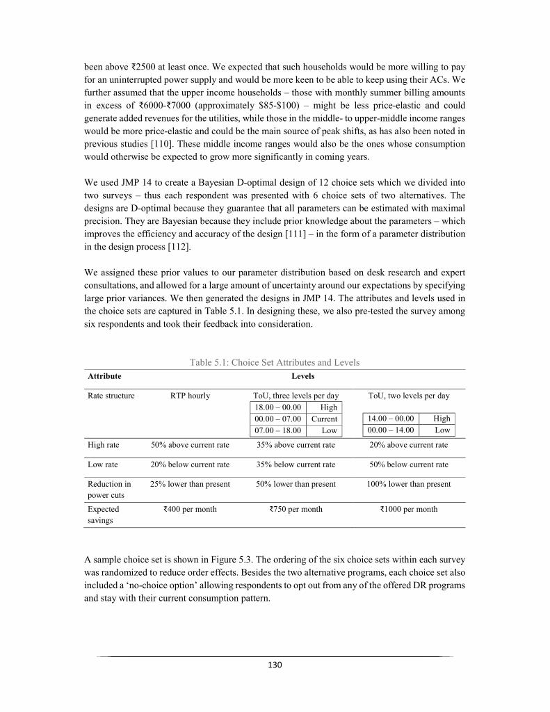
130

been above ₹2500 at least once. We expected that such households would be more willing to pay for an uninterrupted power supply and would be more keen to be able to keep using their ACs. We further assumed that the upper income households – those with monthly summer billing amounts in excess of ₹6000-₹7000 (approximately $85-$100) – might be less price-elastic and could generate added revenues for the utilities, while those in the middle- to upper-middle income ranges would be more price-elastic and could be the main source of peak shifts, as has also been noted in previous studies [110]. These middle income ranges would also be the ones whose consumption would otherwise be expected to grow more significantly in coming years. We used JMP 14 to create a Bayesian D-optimal design of 12 choice sets which we divided into two surveys – thus each respondent was presented with 6 choice sets of two alternatives. The designs are D-optimal because they guarantee that all parameters can be estimated with maximal precision. They are Bayesian because they include prior knowledge about the parameters – which improves the efficiency and accuracy of the design [111] – in the form of a parameter distribution in the design process [112]. We assigned these prior values to our parameter distribution based on desk research and expert consultations, and allowed for a large amount of uncertainty around our expectations by specifying large prior variances. We then generated the designs in JMP 14. The attributes and levels used in the choice sets are captured in Table 5.1. In designing these, we also pre-tested the survey among six respondents and took their feedback into consideration.

Table 5.1: Choice Set Attributes and Levels Attribute Levels

Rate structure RTP hourly ToU, three levels per day 18.00 – 00.00 High 00.00 – 07.00 Current 07.00 – 18.00 Low

ToU, two levels per day

14.00 – 00.00 High 00.00 – 14.00 Low

High rate 50% above current rate 35% above current rate 20% above current rate

Low rate 20% below current rate 35% below current rate 50% below current rate

Reduction in power cuts

25% lower than present 50% lower than present 100% lower than present

Expected savings

₹400 per month ₹750 per month ₹1000 per month

A sample choice set is shown in Figure 5.3. The ordering of the six choice sets within each survey was randomized to reduce order effects. Besides the two alternative programs, each choice set also included a ‘no-choice option’ allowing respondents to opt out from any of the offered DR programs and stay with their current consumption pattern.

131

Figure 5.3: Sample Choice Set

The survey was designed in English; since we expected that most respondents in our target segments would be comfortable with the language, this did not significantly increase the risk of selection bias40. The questionnaire consisted of 30 questions and was split into 4 parts. Part one listed questions about which part of the NCR the respondent lived in, along with a few questions about her electricity profile, such as appliance ownership, average power cuts, availability of power backup systems, and average monthly bills in the summer. Part two presented respondents with psychological profile questions, with scaled responses, to gauge their attitudes towards data privacy, convenience, technology, the environment, and their political affiliations. The ordering of these questions within part two was randomized. Part three included the choice exercise, and was randomly presented before or after part two, to further minimize order effects. In this part, we first also listed the respondents’ existing tariff structures as a reminder to them – the average rate in the two highest rate slabs across the five regions is ₹6.5 per kWh – and explained the structure of the choice set exercise as well as the potential for savings through DR41. Part four concluded with some

40 12% of Indians were English speakers in 2011; the overall English-speaking population was expected to quadruple in a decade, and the percentage of English speakers increases significantly among urban regions and higher income populations [113] 41 The average peak demand savings, across DR trials, has been about 10%, complementing energy efficiency initiatives [114], and when avoided generation costs and over-drawing penalties are passed through to customers, the savings can be significant [115]

132

demographic questions. All questions were phrased in neutral language to minimize respondent manipulation, and we attempted to reduce potential hypothetical bias by explaining the real-life potential for such programs. The full survey is listed in Appendix 5-A. We conducted the survey through December 2018 and January 2019. To obtain these responses, the survey was disseminated online through Qualtrics. We used the following channels of distribution: (i) personal contacts as well as their contacts; (ii) select customers registered with one of the distribution utilities in Delhi – BSES Yamuna – through an employee; (iii) present and former clients of a local real estate agent; (iv) Facebook communities for Delhi, Gurgaon, and Noida; (v) alumni networks of two academic institutions in Delhi; and (vi) other social media, such as LinkedIn, Twitter, and Reddit. This may be viewed as a blend of random, convenience, and snowball sampling. 5.4 Results 5.4.1 Sample Statistics All the respondent data was anonymous and confidential. Although we do not have information about the non-response rates due to the nature of survey distribution, overall, a total of 360 people filled out the survey. Of these, 278 were living in one of the five regions of the NCR under study. From these 278, 21 did not own any ACs, 32 had never had an electricity bill amount of above ₹2500, and 11 fell under both these categories. These 42 were thus ineligible for the choice set exercise. Of the remaining 236 eligible respondents, 167 (70.76%) completed the choice set exercise. The demographic details of these final 167 respondents are captured in Table 5.2 below. It is seen that most respondents were between 25 and 55 years in age, and the sample was skewed towards male respondents. Given the targeted nature of our survey, the sample was expectedly highly educated and fell under the higher income brackets, compared to the Delhi per capita of ₹27,400 per month [116].

133

Table 5.2: Respondent Demographics (N = 167) Characteristic Level Respondents Percentage Age (in years) [1] 18-24

[2] 25-39 [3] 40-54 [4] 55-64 [5] 65 and above

11 74 35 20 17

7.01% 47.13% 22.29% 12.74% 10.83%

Gender [1] Female [2] Male

43 112

27.74% 72.26%

Net monthly household income [1] <₹40,000 [2] ₹40,001-₹60,000 [3] ₹60,001-₹90,000 [4] ₹90,001-₹150,000 [5] ₹150,001-₹250,000 [6] >₹250,000

15 5 19 26 26 37

11.72% 3.91%

14.84% 20.31% 20.31% 28.91%

Educational degree attained [1] High school [2] Bachelor’s [3] Master’s or higher

5 41 103

3.36% 27.52% 69.13%

Car ownership [1] None [2] One car [3] Two cars [4] Three or more cars

13 71 53 21

8.23% 44.94% 33.54% 13.29%

Employment of domestic help [1] None [2] At least 1 person part-time [3] At least 1 person full-time

16 86 57

10.06% 54.09% 35.85%

Housing type [1] Apartment [2] Independent floor [3] Independent house

80 33 46

50.31% 20.75% 28.93%

Number of people in household [1] 1-2 people [2] 3-4 people [3] 5-6 people [4] >6 people

39 74 33 12

24.68% 46.84% 20.89%

7.59% Home ownership [1] Rent

[2] Own [3] Other

44 112 3

27.67% 70.44%

1.89% The electricity profiles of these respondents are captured in Table 5.3. Most respondents lived in Delhi or Gurgaon and owned three or more room ACs. 95% faced summertime power outages of under four hours per day, and 90% of them had at least one type of power backup system at home.

134

Table 5.3: Respondent Electricity Usage Profiles (N = 167) Electricity Profile Question Level Respondents Percentage Part of National Capital Region (NCR)

[1] Delhi [2] Gurgaon [3] Noida [4] Faridabad [5] Ghaziabad

76 65 16 2 8

45.51% 38.92%

9.58% 1.20% 4.79%

Number of air conditioners at home [1] One [2] Two [3] Three or more

19 36 112

11.38% 21.56% 67.07%

Monthly electricity bills amount in summer

[1] <₹2,500 [2] ₹2,500-₹5,000 [3] ₹5,000-₹7,500 [4] ₹7,500-₹10,000 [5] >₹10,000

16 55 37 28 28

9.76% 33.54% 22.56% 17.07% 17.07%

Other heavy appliances at home [1] One [2] Two [3] Three [4] Four

15 89 45 18

8.98% 53.29% 26.95% 10.78%

Average daily power cuts in summer [1] 0-2 hours [2] 2-4 hours [3] 4-6 hours [4] Above 6 hours

127 30 6 2

76.97% 18.18%

3.64% 1.21%

Power backup system [1] None [2] Diesel-based [3] UPS/Inverter [4] Community backup

17 11 85 54

10.18% 6.59%

50.90% 32.33%

Rooftop solar PV panels [1] No [2] Yes/Maybe

146 20

87.95% 12.05%

Lastly, some of the socio-psychological values of the respondents are captured in Table 5.4. Most were not very concerned about data privacy, suggesting that they may not be resistant to the introduction of smart meters. While 61% were very concerned about the environment, only 42% expressed a willingness to personally act on their concerns. A larger number of respondents seemed to be politically liberal than conservative, based on their news viewership, and most were comfortable with new technologies.

135

Table 5.4: Respondent Values (N = 167) Socio-Psychological Value Level Respondents Percentage Privacy 1 (On activities being recorded)

[1] Not at all comfortable [2] Not very comfortable [3] Fairly comfortable [4] Very comfortable

2 27 61 73

1.23% 16.56% 37.42% 44.79%

Privacy 2 (On personal information being stored)

[1] Not at all comfortable [2] Not very comfortable [3] Fairly comfortable [4] Very comfortable

2 13 66 83

1.22% 7.93%

40.24% 50.61%

Environment 1 (Importance of environment to respondent)

[1] Not at all important [2] Not very important [3] Neutral [4] Somewhat important [5] Very important

6 2 11 45 99

3.68% 1.23% 6.75%

27.61% 60.74%

Environment 2 (Willingness to spend on sustainable products)

[1] Completely disagree [2] Somewhat disagree [3] Neutral [4] Somewhat agree [5] Completely agree

6 13 11 65 68

3.68% 7.97% 6.75%

39.88% 41.72%

Convenience (Preference for shopping online)

[1] Completely disagree [2] Somewhat disagree [3] Neutral [4] Somewhat agree [5] Completely agree

15 26 43 59 20

9.20% 15.95% 26.38% 36.20% 12.27%

Political leaning (Preferred news channel)

[1] Right-leaning [2] Left-leaning [3] Others

41 70 52

25.15% 42.94% 31.90%

Technology 1 (On new technologies being better)

[1] Completely disagree [2] Somewhat disagree [3] Neutral [4] Somewhat agree [5] Completely agree

2 30 35 75 22

1.22% 18.29% 21.34% 45.73% 13.41%

Technology 2 (Ease of use of new technology)

[1] Completely disagree [2] Somewhat disagree [3] Neutral [4] Somewhat agree [5] Completely agree

0 23 27 78 36

0.00% 14.02% 16.46% 47.56% 21.95%

5.4.2 Logit Model Results We estimated the MNL model with main effects only, using Firth bias correction [117] – using Firth’s penalized maximum likelihood in small sample problems provides estimates with a smaller bias and variance than estimates obtained using ordinary maximum likelihood. We then confirmed the estimates using the mixed logit method, which yields a better goodness-of-fit, and which we used in the remainder of the analysis. The results of these two models are captured in Table 5.5.

136

Table 5.5: Parameter Estimates and Goodness-of-Fit for Main Effects Model a Effect MNL Mixed logit Mean Estimate Std. Dev Mean Estimate Std. Dev Rate structure [RTP] -0.1454* 0.0688 -4.7249** 1.6561 Rate structure [ToU 3 times] 0.0861* 0.0537 3.0103** 1.3057 High rate -1.1599*** 0.4190 -43.7282** 9.4445 Low rate 0.8199** 0.3694 24.0235** 6.8355 Reduction in power cuts 0.6497*** 0.1658 25.4045** 4.2851 Expected monthly savings 0.0009*** 0.0002 0.0196** 0.0062 No choice indicator 0.1648 0.2800 -71.8557 18.1288 Goodness of Fit Measure Value Value -2 * LL 2001.8002 134.5537 Total Iterations: 15000

a P < 0.01: ***|| P < 0.05: **|| P < 0.1: * The coefficients of real-time pricing and three-rates-a-day ToU represent their utilities relative to the two-rates-a-day ToU structure. Expectedly, of the three rate structures, the real-time pricing had the lowest utility to respondents, since it would require the most effort to track. However, although we had expected the two-rates-a-day ToU to be preferable to the three-rates-a-day ToU as it was simpler in design, the three-rates-a-day ToU came out with the highest utility across rate structures, reflecting the fact that it offered 6 hours of peak pricing, unlike the 10 hours of peak pricing in the two-rates-a-day ToU plan. Respondents attached the greatest importance to the upper price band, and to the reductions they could expect in power cuts – these indicate the high value people attach to security of supply and price considerations. Based on these mixed logit estimates, using Equation 4, we estimate the monthly savings that respondents would require for a change in each of the attributes, shown in Table 5.6, assuming that the rate changes and reductions in power cuts are linear in utility42.

Table 5.6: Monthly Savings Required for Changes

Attribute Change Desired Savings Required Rate Structure ToU 3 rates - RTP ₹ 393.14 Rate Structure ToU 3 rates - ToU 2 rates ₹ 65.85 High Rate 10% increase ₹ 222.24 Low Rate 10% reduction -₹ 122.10 Reduction in Power Cuts 10% reduction -₹ 129.12

We then test for subject effects using the mixed logit model, and the results of this full model are captured in Table 5.7. 42 We tested for exponential utilities in the mixed logit model, but the goodness-of-fit and significance of parameter estimates was found to be lower in those cases

137

Table 5.7: Parameter Estimates and Goodness-of-Fit for Overall Model b Effect Posterior

Mean Posterior Std. Dev

Subject Std. Dev

Main Effects Rate structure [RTP] -9.5297** 4.7590 34.3279 Rate structure [ToU 3 times] 6.6491** 2.8787 23.7150 High rate -69.4249** 18.1029 33.5181 Low rate 46.1991** 17.8895 85.9705 Reduction in power cuts 38.6684** 10.4992 21.6869 Expected monthly savings 0.0642* 0.0344 0.0834 No choice indicator -24.5196** 10.6798 6.1153

Subject Effects High rate * Monthly bills [2] -31.6950 22.2196 56.5519 High rate * Monthly bills [3] -57.7057** 22.2951 13.7876 High rate * Monthly bills [4] -91.1971** 30.1354 7.0693 High rate * Monthly bills [5] -23.1002 55.3610 4.3074 Reduction in power cuts * Age [2] 21.8808 13.0266 10.9530 Reduction in power cuts * Age [3] -17.2219* 8.9144 11.6467 Reduction in power cuts * Age [4] -30.4321 23.0164 2.6994 Reduction in power cuts * Age [5] -29.3362** 14.3113 2.2346 Reduction in power cuts * Income [2] 13.4181 18.2701 30.9496 Reduction in power cuts * Income [3] 22.3316* 11.7106 24.7583 Reduction in power cuts * Income [4] 25.7021** 11.6405 4.1048 Reduction in power cuts * Income [5] 56.0497** 11.6642 5.9376 Reduction in power cuts * Income [6] 63.2032** 23.2532 3.8995 Expected savings * Environment 1 [2] 0.1868** 0.0794 0.2356 Expected savings * Environment 1 [3] 0.1758** 0.0881 0.1382 Expected savings * Environment 1 [4] 0.0595* 0.0329 0.0610 Expected savings * Environment 1 [5] 0.0578 0.0426 0.0529 No choice indicator * Convenience [2] -23.6463** 11.8685 5.3641 No choice indicator * Convenience [3] -171.1601** 63.2396 116.6273 No choice indicator * Convenience [4] 33.5092** 14.3121 6.0846 No choice indicator * Convenience [5] -491.1501* 253.4644 71.0172 No choice indicator * Home ownership [1] 34.1568** 15.9839 4.0730 No choice indicator * Home ownership [2] 28.3893** 11.3569 1.3049 Goodness of Fit Measure Value -2 * Average LL Total Iterations: 15000, Burn-in Iterations: 7500

69.1011

b P < 0.01: ***|| P < 0.05: **|| P < 0.1: * 5.5 Discussion and Policy Implications 5.5.1 Discussion of Estimates The overall model in Table 5.7 shows that the proportional utilities of the five attributes in relation to each other remain similar to the main effects model. However, the respondent profiles do affect the preferences among the various attribute levels.

138

The disutility from the high rate increases as respondents’ monthly bill amounts increase, indicating a greater unwillingness to risk higher bill amounts. The high coefficients also indicate – in line with literature [46] – that respondents are very sensitive to prices and / or loss-averse, particularly if they’re already paying a lot. Younger respondents tend to derive a greater utility from reductions in power cuts. 13 of the 17 respondents who didn’t have a power backup system, and 22 of the 38 who faced summertime power cuts above 2 hours per day, fell in the first and second age categories, which may partly explain this trend. Yang et al. [118] had found, using survey data, that younger consumers are more likely to shift to ToU pricing programs than older ones, although their analysis wasn’t related to energy security. Alongside security of supply issues, younger populations also tend to use more technological appliances [119] and may thus be more reliant on electricity for entertainment purposes. Higher levels of income within this middle to upper-income sample also correlate to a greater utility derived from reductions in power cuts. An average respondent with a household income of more than ₹250,000 per month is willing to pay ₹984 per month more for eliminating power cuts than an average respondent with a household income of under ₹40,000 per month. It is possible that the richest populations are more willing to spend money on comfort. In line with this, 33 of the 63 respondents (52.4%) with a stated income of above ₹150,000 per month valued convenience highly, compared with the sample average of 48.4%. This corresponds to our initial expectations, that upper-income households would be more willing to pay for an uninterrupted power supply, and could generate added revenues for utilities. It is also in line with other literature [120,121], based on methods such as choice experiments and secondary survey data, which shows that higher incomes lead to greater values for comfort and convenience and correlates negatively with energy curtailment behavior. The utility from expected monthly savings (arising through shifts in electricity use) was increasing at a decreasing rate with increases in the levels of environmental concern However, the increase in utility was marginal and would not substantially affect the savings required, suggesting that people would not be willing to financially sacrifice too much in the interest of benefitting the environment. This was also seen from the relationship between the first and the second environmental questions, on the concern for the environment and the willingness to spend on more sustainable products, in Table 4. It runs against previous findings [45] from developed country contexts, although the potential environmental benefits of DR were not explained in our study. People derived a lower utility from staying on the current plan if they owned their homes rather than renting them – Ericson [44] suggests that house-dwellers might have a greater ability to reduce consumption than apartment-dwellers, and we observe a strong correlation between type of dwelling and home ownership in our sample (χ2 value 145.5 at 4 degrees of freedom for a p-value of 0.0001) – and if they valued convenience more highly. This went against expectations, since staying with the status quo would inconvenience people less than shifting to a new tariff structure that requires a more active monitoring of rates.

139

We did not find significant effects for education rates, the presence of domestic help such as maids, power cuts and backup systems, values towards privacy and technology. We expect that response bias, sample selection and size, and cultural differences may have played a role in these omissions. Further, to reduce cognitive burden and given the low market penetration rates, we did not include smart appliances in our study. In discussing these results, we note that the Indian economy is growing rapidly, implying that more people will eventually move into the upper income categories where expected price elasticity might be lower, as seen from the value of reduced power cuts, yielding greater revenues for the utilities. At the same time, many more people may also enter the middle- to upper-middle income ranges, creating the potential for significantly higher peaks if consumption patterns aren’t meaningfully shifted. 5.5.2 Cluster Analysis of Preferences We further study preference heterogeneity by adopting a hierarchical clustering method to identify preference clusters, similar to the approaches Pinto et al. [122] and Luyten et al. [99] used as complements to choice exercises. Clustering sorts objects according to their similarity on desired dimensions and identifies groups that maximize within-group similarity and minimize between-group similarity [123]. For the dimensions, we use the subject-level coefficients for each attribute from the main-effects mixed logit model. Taking the cubic clustering criterion values [124,125] into account, we specify a four-cluster scheme, and identify the characteristics of the respondents within each cluster to examine differences between them. These characteristics are shown in Table 5.8, together with the averaged values of the attribute coefficients within each cluster. We do not pursue this exploratory analysis with confirmatory approaches such as regressions to determine predictors of cluster membership.

Table 5.8: Cluster Analysis Based on Preferences Sample

N=167 Cluster 1

N=34 Cluster 2

N=39 Cluster 3

N=27 Cluster 4

N=67 Demographic Age (55 years or above) 22.15% 18.18% 25.64% 33.33% 18.18% Gender (Female) 25.74% 18.18% 23.08% 25.93% 30.30% Income (≥ ₹150,000) 37.72% 27.27% 53.84% 40.74% 31.82% Car Ownership (≥ 3) 12.57% 18.18% 10.26% 14.81% 10.61% Number of people (≥ 5) 26.95% 36.36% 25.64% 22.22% 25.76% Home ownership 67.06% 69.69% 66.67% 70.37% 65.15% Electricity Profile People in Delhi 45.51% 48.48% 43.59% 44.44% 43.94% Number of ACs (≥ 3) 67.06% 63.63% 69.23% 74.07% 65.15% Monthly bills (≥ ₹7500) 33.53% 36.36% 28.20% 40.74% 31.82% Daily power cuts (> 2 hrs.) 22.75% 24.24% 28.20% 25.93% 18.18% Continued on next page

140

Table 5.8 (Continued) Sample

N=167 Cluster 1

N=34 Cluster 2

N=39 Cluster 3

N=27 Cluster 4

N=67 Value Privacy 1 [Level 3,4] 80.24% 87.88% 76.92% 66.67% 83.33% Environment 2 [Level 4,5] 79.64% 69.70% 87.18% 77.78% 80.30% Convenience [Level 4,5] 47.31% 42.42% 46.15% 51.85% 46.97% Technology 1 [Level 4,5] 58.08% 51.51% 69.23% 40.74% 63.64% Utility Coefficients Rate Structure (RTP) -4.50 -3.03 -1.30 -20.88 -0.43 Rate Structure (ToU 3) 3.13 -0.12 5.33 16.44 -1.97 High Rate -48.90 -72.41 -21.23 -82.91 -39.59 Low Rate 23.41 -9.65 19.95 4.77 49.63 Reduction in Power Cuts 26.84 28.07 74.28 5.16 7.08 Expected Savings 0.02 -0.07 -0.02 0.04 0.08

We see that Cluster 1 had more negative preference weights overall, and was more likely to select the ‘no choice’ option i.e. reject the proposed DR structures and remain on the current tariff plan. Relatively, this cluster had the most number of male respondents as well as the lowest income earners among the middle to upper-income sample. The household size was the largest in this cluster, and AC ownership was lower. Respondents had the lowest privacy concerns, lowest scores on convenience, and lowest willingness to spend more for environmentally-friendly products. Cluster 2 had a strong preference for reductions in power cuts and in general experienced less disutility from the higher peak rates. This cluster had the highest incomes, though car ownership was lower. Respondents in this cluster were most willing to spend more on environmentally-friendly products, and were very comfortable with new technologies. Cluster 3 exhibited very strong preferences for the rate structures and higher peak rates, and comparatively weak preferences for reductions in power cuts. This cluster had more older respondents, smaller household sizes, and the highest rates of home and car ownership. Respondents also owned more ACs and had larger monthly electricity bills. They had stronger privacy concerns, and greater preferences for convenience, but were least comfortable with new technologies. Lastly, cluster 4 – with the largest population – had comparatively strong preferences for the lower off-peak rates and for the expected savings, and were relatively indifferent to the rate structures. This cluster included more younger respondents, as well as more female respondents. They had lower incomes and fewer cars, relative to the rest of the sample, and the lowest rates of home ownership. Respondents in this cluster also faced the fewest power cuts. Though we note that certain characteristics, such as home ownership rates, were not significantly different across the clusters, these clusters indicate that even among the middle to upper-income households in the Delhi-NCR region, different groups within the sample may have heterogenous

141

concerns, likely shaped by their different characteristics. These varying concerns will have different effects on future DR adoption. 5.5.3 General Utility-Based Options The model results demonstrate that DR can be a feasible option in India, from the point of view of customer acceptance. Yan et al. [126], in a review of price-based DR, conclude that with smart metering technologies, pricing signals can be an effective instrument for peak demand reductions, reliability management, and emissions and cost reductions. With this in mind, we use our results to propose specific pricing signals for the Indian market. In doing so, we take two independent approaches to offering policy suggestions. First, we use the main effects model to derive four DR structures that achieve a high general utility. We apply the parameter estimates of the main effects mixed logit model from Table 5 to the most preferred levels of the attributes that we used in our choice sets: (i) a three-rates-a-day ToU rate, (ii) an upper rate of 20% above current levels, (iii) a lower rate of 50% below current levels, (iv) a 100% reduction in power cuts, and (v) a ₹1000 in monthly bill savings. This yields a total utility of 51.28. Although this is an unlikely combination of attribute levels, the average utility, using the parameter estimates under the main effects model, of the 24 alternatives presented to respondents across choice sets is 21.29, and the standard distribution of their utility is 8.73. Based on these measures, and assuming a normal distribution, we set a target to achieve a utility acceptable at the 90% level (right-tailed p-value of 0.1) i.e. 32.47, and present four possible DR structures that approximately achieve this level of utility and that could feasibly be implemented among a general population, not taking into account the specific subject effects captured in the overall model. These four structures are presented in Table 5.9. For each proposed structure, we calculate the relative importance (RI) of each attribute, A – and its monetary value – within the structure, based on Equations 5 and 6.

RIA = [ |UA| / ∑A=14 |UA | ] * 100 (5)

ValueA = UA / ∑A=1

4 UA * (Expected Savings) (6)

Table 5.9: Potential DR Structures based on Main Effects Attribute Structure 1 Structure 2 Structure 3 Structure 4 Rate structure Relative Importance Value

ToU 2 5.84% ₹84.33

ToU 3 7.69% ₹76.45

ToU 3 6.52% ₹90.48

RTP 10.25% -₹160.45

High rate Relative Importance Value

+15% 22.32% -₹322.60

+20% 22.34%

-₹222.10

+30% 28.40%

-₹394.28

+20% 18.98% -₹296.99

Continued on next page

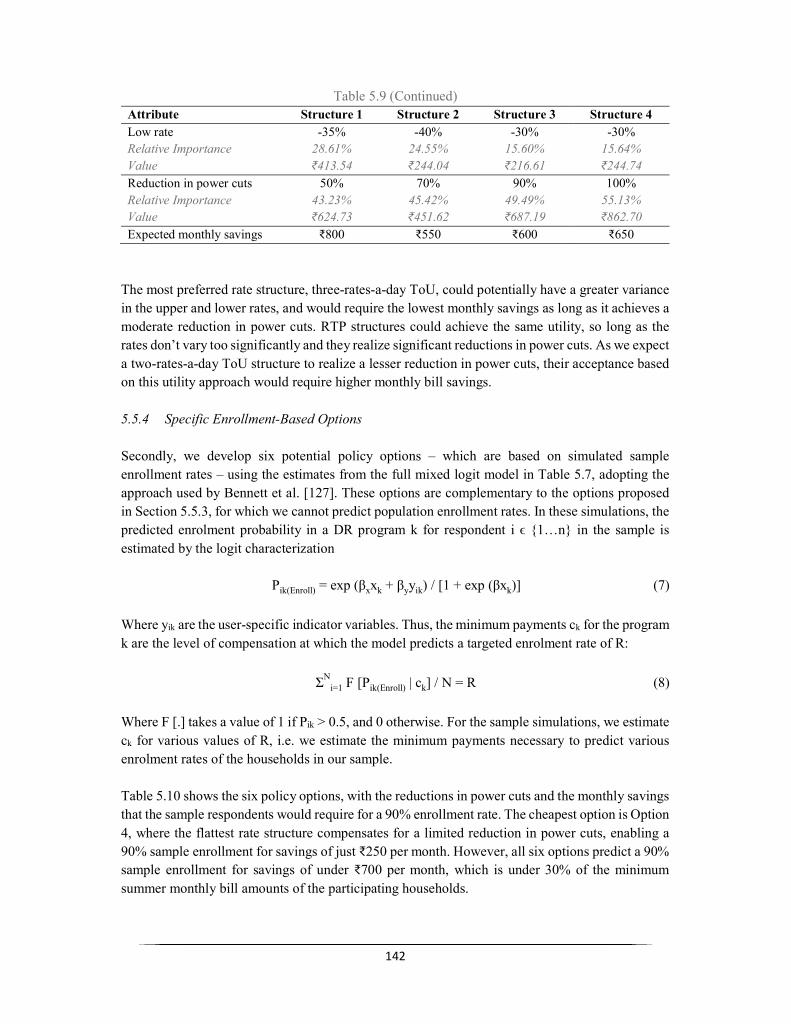
142

Table 5.9 (Continued) Attribute Structure 1 Structure 2 Structure 3 Structure 4 Low rate Relative Importance Value

-35% 28.61% ₹413.54

-40% 24.55% ₹244.04

-30% 15.60% ₹216.61

-30% 15.64% ₹244.74

Reduction in power cuts Relative Importance Value

50% 43.23% ₹624.73

70% 45.42% ₹451.62

90% 49.49% ₹687.19

100% 55.13% ₹862.70

Expected monthly savings ₹800 ₹550 ₹600 ₹650 The most preferred rate structure, three-rates-a-day ToU, could potentially have a greater variance in the upper and lower rates, and would require the lowest monthly savings as long as it achieves a moderate reduction in power cuts. RTP structures could achieve the same utility, so long as the rates don’t vary too significantly and they realize significant reductions in power cuts. As we expect a two-rates-a-day ToU structure to realize a lesser reduction in power cuts, their acceptance based on this utility approach would require higher monthly bill savings. 5.5.4 Specific Enrollment-Based Options Secondly, we develop six potential policy options – which are based on simulated sample enrollment rates – using the estimates from the full mixed logit model in Table 5.7, adopting the approach used by Bennett et al. [127]. These options are complementary to the options proposed in Section 5.5.3, for which we cannot predict population enrollment rates. In these simulations, the predicted enrolment probability in a DR program k for respondent i ϵ {1…n} in the sample is estimated by the logit characterization

Pik(Enroll) = exp (βxxk + βyyik) / [1 + exp (βxk)] (7) Where yik are the user-specific indicator variables. Thus, the minimum payments ck for the program k are the level of compensation at which the model predicts a targeted enrolment rate of R:

ΣNi=1 F [Pik(Enroll) | ck] / N = R (8)

Where F [.] takes a value of 1 if Pik > 0.5, and 0 otherwise. For the sample simulations, we estimate ck for various values of R, i.e. we estimate the minimum payments necessary to predict various enrolment rates of the households in our sample. Table 5.10 shows the six policy options, with the reductions in power cuts and the monthly savings that the sample respondents would require for a 90% enrollment rate. The cheapest option is Option 4, where the flattest rate structure compensates for a limited reduction in power cuts, enabling a 90% sample enrollment for savings of just ₹250 per month. However, all six options predict a 90% sample enrollment for savings of under ₹700 per month, which is under 30% of the minimum summer monthly bill amounts of the participating households.

143

Table 5.10: Policy Options for 90% Sample Enrollment # Rate Structure High Rate Low Rate Reductions in

Power Cuts Monthly Savings

1 RTP Up to 30% higher Up to 20% lower 30% ₹400 2 RTP Up to 40% higher Up to 40% lower 80% ₹650 3 ToU 2 times 40% higher 50% lower 40% ₹550 4 ToU 2 times 20% higher 10% lower 20% ₹250 5 ToU 3 times 35% higher 20% lower 40% ₹500 6 ToU 3 times 50% higher 35% lower 60% ₹700

Figure 5.4 additionally shows the predicted enrollment rates for these policy options at various levels of expected monthly savings. It is seen that Options 2 and 6 – with higher peak rates but substantial reductions in power cuts – would have the highest enrollment rates when the expected monthly savings are negligible. In the middle brackets of expected savings, around ₹100-₹400 per month, options 1 and 4 – offering both the lowest peak rates and least reductions in power cuts – would enroll the greatest shares of the sample. Options 3 and 5 would witness stable increases in enrollment. Option 1, offering RTP with higher off-peak rates and fewer reductions in power cuts, is the least attractive in the absence of significant savings.

Figure 5.4: Sample Enrollment Rates for Policy Options

We note that the predicted enrollment rates would be dependent not just on the levels of expected savings, but also on the DR structures being able to offer these predicted reductions in power cuts. Further, we caution that since the sample may not be representative of the middle and upper-income populations in the city, these options can serve as indicative guideposts rather than definitive recommendations.

0%

10%

20%

30%

40%

50%

60%

70%

80%

90%

100%

0 50 100 150 200 250 300 350 400 450 500 550 600 650 700

ENRO

LLM

ENT

RATE

MONTHLY SAVINGS (IN ₹)

1 2 3 4 5 6

144

5.5.5 Economic Value of Demand Response Implementation Lastly, we explore the economic value – to households and utilities – of shifts in consumption once a dynamic pricing program is introduced. We however do not look at the costs of implementing such a program. We choose the rates structures outlined in Option 5 above, since it falls in the middle of the other options in terms of enrollment rates, as seen in Figure 5.4. We consider the effects on Delhi alone, and do not include the other regions in this study. There were about 3.7 million households in Delhi in 2009-10 [128]; we expect that with urbanization, population growth rates, and nuclearization of families, there are currently around 4 million households. We then assume that the DR program is applied to the richest 20% of Delhi’s population, similar to the set-up in this choice experiment, which comes to about 800,000 households. We expect that these 20% of households are responsible for about 45% of the city’s residential electricity consumption, similar to the shares of income mentioned in Section 5.3.2. In Option 5, the difference between the peak (35% higher, or ₹8.8) and off-peak (20% lower, or ₹5.2) rates is ₹3.6 per kWh. Given that each room AC uses an average of 1.8 kW [129,130], then for each hour that an AC’s usage is shifted from peak to off-peak hours, the household bill savings would come to (i) ₹6.48, relative to consuming at peak hours, and (ii) ₹2.34, relative to current rates. Thus, if a household shifts consumption of 1 AC for two hours each evening, the monthly savings for a household that is consuming 407 kWh come to about (i) ₹390, compared to consuming at peak hours (10.47% of a current average bill), or (ii) ₹140, compared to consuming under the current tariff structure (3.76% of a current average bill). These savings can become more significant if further flexibility is induced in other ACs, water heaters, washing machines, and other appliances. Further, the residential sector accounts for 44% of Delhi’s total electricity demand [131] – for simplicity, we assume it constitutes 50%, or roughly 3500 MW, of the 7000 MW peak43. If the top 20% of households are responsible for 45% of total residential consumption, and 50% of the shares at peak hours, then they would account for 1750 MW of the peak demand. Shifts of even 20%, which have been observed in DR programs in other countries [114,132], could thus lead to reductions in peak demand of up to 350 MW, or 5% of the total peak. 5.6 Conclusion This paper used a discrete choice experiment approach to test the feasibility of implementing a dynamic pricing-based demand response program in the residential sector in India. India is an emerging economy with a large low-income population, and with 300 million people still without regular access to electricity. Additionally, it is experiencing high rates of economic growth, high rates of increase in consumption, and consequently large increases in greenhouse gas emissions. The creates the incentive for using DR to improve the security of supply, particularly

43 Chapter 4 had noted that residential shares of peak demand can be higher than their shares of total demand

145

with India’s ambitious renewables targets. The opportunity for implementing such DR programs comes from India’s smart grid ambitions and its smart metering targets. The analysis focused on the national capital region of Delhi. This was due to considerations of homogeneity – each state in India has its own electricity tariff structure – and socio-cultural comparability. With a population of 26 million people, an implementation even in this region alone can potentially yield sizeable effects, particularly as Delhi has the highest per capita electricity consumption rates in the country. The expectation is that any peak reductions can be used to improve electricity access to underserved populations, while any additional revenues to utilities can be used to improve the provision of electricity services and the grid infrastructure. The target population was middle to upper-income households who had a summertime monthly bill in excess of ₹2500 and who owned at least one room AC. We obtained 167 usable responses for our analysis, where each respondent was presented with six choice sets of two alternatives. Each alternative was comprised of five attributes with three possible levels. The results showed that respondents preferred ToU pricing to RTP structures, possibly because they are easier to manage. Within ToU structures, they preferred the three-rate structure to the two-rate structure, perhaps because the former offered a fewer number of hours of peak pricing than the latter. In general, however, respondents attached a lower utility to the different types of rate structures than to the remaining attributes. Although the off-peak rates weren’t as important, respondents exhibited a strong preference for lower peak time rates, particularly if their monthly electricity bills were already high. This indicated a greater aversion to loss and a greater unwillingness for potentially further inflating existing bill amounts. Respondents attached a high value to reductions in power cuts, indicative of the extent of supply-side problems. Younger and higher income respondents in particular attached a higher utility to such reductions, owing to a mix of greater technological appliance usage and lower ownership of power backup systems among the former, and a greater value of convenience among the latter group. Although respondents who were more concerned about the environment attached a lower utility to the required monthly savings, this amount was not substantial and indicated that environmental concern does not necessarily translate to action. This was in line with the risk of hypothetical bias that is faced by choice experiments, and also suggests that environmental issues are a secondary consideration. A cluster analysis grouped respondents into four clusters based on similarities in their preferences and demonstrated that respondents that exhibit similar preferences also share similar characteristics that are distinct from those of respondents in other clusters. Based on the results of the analysis, the paper then presented a number of potential DR structures that could be feasibly implemented, four of which were designed to achieve a high general utility, and six that were designed to achieve a 90% enrollment among the sample respondents. Lastly, it offered a rough estimate of the potential benefits – to households and utilities – of implementing one of these structures.

146

Overall, the analysis demonstrates that a time-of-use pricing-based demand response program could be feasible even in a developing country context, particularly when it is designed for middle to upper-income households, in line with the political economy of the national electricity sector. While framing it as an environmental solution may help to some extent, the key concerns for the local population are expected savings and reductions in power cuts. Thus, any DR program would have to clearly be able to address people’s price sensitivities and security of supply concerns. We acknowledge that we did not offer smart appliances and smart meters in our hypothetical choice exercise, although their availability may also affect the desirability of such programs, and the potential impacts on power cuts were hypothetical. Aside from the risk of hypothetical bias, discrete choice experiments should also be interpreted differently from actual trials, because the short run and long run price elasticities are measurably different due to behavioral learning over time, and due to stock changes (e.g. buying smart or more efficient appliances) [133,134]. Price-based DR programs also run the risk that they may attract consumers who benefit without responding to the price, simply because they already have a favorable consumption pattern [45], although this has not been found to be a significant factor in previous analyses [44]. However, we believe that the potential benefits of choice experiments, particularly as early indicators of market feasibility, outweigh their limitations. Future studies looking at the Indian context may consider applying similar methods to other cities, in order to consider the design requirements for a national roll-out, and may look at the techno-economic feasibility of actually implementing such programs. Additionally, further studies may also explore the potential for DR in other developing countries using similar approaches, in order to understand what lessons may be replicable across developing country contexts.

147

Appendix 5-A: Survey Questionnaire Dear survey participant, We really appreciate you filling out our survey. This survey has 30 multiple-choice questions, and should take under 10 minutes to complete. Your responses are vital to our research on improving the provision of electricity to your home. Findings from this research could help in designing future electricity tariffs. All answers are strictly confidential and anonymous. To acknowledge your effort, when you complete the survey, we will donate an amount of ₹20/- on your behalf to the GiveIndia Foundation. Thank You Part 1 Q: Which part of the NCR do you live in?

Delhi Gurgaon Noida Ghaziabad Faridabad None of these

Q: Do you have any air conditioners (ACs) installed in your home?

No Yes, I have one AC Yes, I have two ACs Yes, I have three or more ACs

Q: Do you have any of the following appliances in your home?

A washing machine A microwave A second refrigerator A clothes dryer None of these

148

Q: What is your approximate monthly electricity billing amount during the summer and monsoon (Apr - Sep)?

< ₹2500 ₹2500-₹5000 ₹5000-₹7500 ₹7500-₹10,000 > ₹10,000 Don’t know

Q: On average, how many hours of power cuts would you say you experience in a day during the summer and monsoon (Apr - Sep)?

0 to 2 hours per day 2 to 4 hours per day 4 to 6 hours per day More than 6 hours per day

Q: Do you have a backup power system at home?

No Yes, diesel genset or generator Yes, UPS or battery inverter Yes, community power backup Other

Q: Do you have rooftop solar PV panels installed in your house?

Yes Maybe No

[Survey proceeds only if respondent lives in Delhi-NCR, has at least 1 AC installed, and has had a monthly billing amount of above ₹2500 at least once] Part 2 Please answer a few questions about your general concerns and preferences. Please remember that your responses will be anonymous and confidential Q: Nowadays, cameras, credit cards, and websites can record your activities for a number of reasons. How do you feel about this?

Very concerned Fairly concerned Not very concerned Not at all concerned

149

Q: Different organizations store personal information about people in their databases. How do you feel about whether your information is being protected by these organizations?

Very concerned Fairly concerned Not very concerned Not at all concerned

Q: On a scale of 1 to 5, with 1 being the lowest and 5 being the highest, how important is protecting the environment to you personally? Q: To what extent do you agree or disagree with the following statement: I am ready to buy environmentally-friendly products, even if they cost say 10% more than the normal brands

Completely disagree Somewhat disagree Neutral Somewhat agree Completely agree

Q: To what extent do you agree or disagree with the following statement: I would usually prefer to shop online instead of going to a store

Completely disagree Somewhat disagree Neutral Somewhat agree Completely agree

Q: Which news channel do you normally prefer to watch?

Republic TV Times Now NDTV CNN Aaj Tak India Today Other

Q: To what extent do you agree or disagree with the statement: New technology is always better than the technology it replaces

Completely disagree Somewhat disagree Neutral Somewhat agree Completely agree

150

Q: To what extent do you agree or disagree with the statement: New technology is usually easy to work with

Completely disagree Somewhat disagree Neutral Somewhat agree Completely agree

Part 3 For the next six questions, please first take a moment to consider your current tariff [Here we offer a summary of the tariff structure of the town respondent is in] With the current electricity infrastructure, you face frequent power cuts and pay high bills. But if your electricity rates could change with time, based on the costs of generating that electricity, you could save a lot of money by adjusting your electricity usage to the rates. This would also reduce power cuts. The next six questions showcase various tariff structures designed for usage above 300 units per month in the summer, and demonstrate how much money you can save with these tariffs. Through your feedback, we try to understand what tariffs you would then be willing to accept. Each tariff structure that we present to you will be based on different levels of these 5 components: [Here we offer a description of the attributes in the following choice sets] In each of the next 6 questions, please choose which of the two tariffs you would prefer, if any. Remember that your current rate is approximately ₹6.50 per unit [Six times over three pages] Q: Please select the tariff that you prefer [Choice set]

Tariff 1 Tariff 2 I wouldn’t choose either option

Part 4 Please answer a few final questions about yourself. As a reminder, these responses will be completely anonymous and confidential

151

Q: Please indicate your age Under 18 years 18 - 24 years 25 - 39 years 40 - 54 years 55 - 64 years 65 years or above I prefer not to answer

Q: Please indicate your gender

Male Female I prefer not to answer

Q: What is the net average monthly income of your household?

Under ₹40,000 ₹40,001 - ₹60,000 ₹60,001 - ₹90,000 ₹90,001 - ₹1,50,000 ₹1,50,000 - ₹2,50,000 Above ₹2,50,000 I prefer not to answer

Q: What is the most recent educational degree you attained?

Secondary school (12th pass) BA, BBA, BSc, BTech, or equivalent MA, MBA, MSc, MTech, or higher I prefer not to answer

Q: Does anyone in your household own a car?

No Yes, I/we own 1 car Yes, I/we own 2 cars Yes, I/we own 3 or more cars

Q: Do you employ a maid or other domestic help?

Yes, at least 1 full-time help Yes, at least 1 part-time help No

152

Q: Including yourself, how many people live in your household (family or flat-mates)? 1-2 3-4 5-6 More than 6

Q: What type of dwelling do you live in?

Apartment Independent floor Independent house

Q: Do you own or rent your current place of accommodation?

Own Rent Other, e.g. staying at relative’s

153

References [1] United States Environmental Protection Agency. Sources of greenhouse gas emissions, https://www.epa.gov/ghgemissions/sources-greenhouse-gas-emissions [accessed 14.01.2019] [2] EnerData. Electricity domestic consumption, https://yearbook.enerdata.net/electricity/electricity-domestic-consumption-data.html [accessed 21.01.2019] [3] International Renewable Energy Agency. Global renewable generation continues its strong growth, https://www.irena.org/newsroom/pressreleases/2018/Apr/Global-Renewable-Generation-Continues-its-Strong-Growth-New-IRENA-Capacity-Data-Shows [accessed 17.01.2019] [4] World Energy Council. (2016). E-storage: Shifting from cost to value. Wind and solar applications. Report. World Future Energy Summit, 1–52. https://doi.org/http://www.worldenergy.org/wp-content/uploads/2013/09/Complete_WER_2013_Survey.pdf [5] E3G. (2014). Energy efficiency as Europe’s first response to energy security. E3G briefing note. https://www.e3g.org/docs/E3G_Briefing_June_2014_Energy_efficiency_as_Europe%e2%80%99s_first_response_to_energy_security.pdf [6] United States Department of Energy. Demand response, https://www.energy.gov/oe/activities/technology-development/grid-modernization-and-smart-grid/demand-response [accessed 11.02.2019] [7] European Commission. (2016). Impact assessment study on downstream flexibility, price flexibility, demand response and smart metering. European Commission, ENER/B3/2015-641. https://ec.europa.eu/energy/sites/ener/files/documents/demand_response_ia_study_final_report_12-08-2016.pdf [8] Dranka, G. G., & Ferreira, P. (2019). Review and assessment of the different categories of demand response potentials. Energy, 179, 280–294. https://doi.org/10.1016/j.energy.2019.05.009 [9] European Commission. Commission proposes new rules for consumer centered clean energy transition, https://ec.europa.eu/energy/en/news/commission-proposes-new-rules-consumer-centred-clean-energy-transition [accessed 14.12.2018] [10] United States Smart Grid Initiative. Smart grid investment grant program, https://www.smartgrid.gov/recovery_act/overview/smart_grid_investment_grant_program.html [accessed 14.12.2018] [11] California Public Utilities Commission. (2016). Decision adopting guidance for future demand response portfolios and modifying decision 14-12-024. CPUC note. http://docs.cpuc.ca.gov/PublishedDocs/Efile/G000/M166/K460/166460832.PDF [12] Michigan Public Service Commission. (2017). Demand response market assessment. MPSC. https://www.michigan.gov/documents/mpsc/MI_Demand_Response_Market_Assessment_20170929_602432_7.pdf

154

[13] Maryland Energy Administration. Demand response and building automation grant program, https://energy.maryland.gov/business/Pages/incentives/drba.aspx [accessed 17.02.2019] [14] SEDC. (2017). Explicit demand response in Europe – Mapping the markets 2017. SEDC. https://www.smarten.eu/wp-content/uploads/2017/04/SEDC-Explicit-Demand-Response-in-Europe-Mapping-the-Markets-2017.pdf [15] Joint Research Center. Smart Grid Projects Map, http://ses.jrc.ec.europa.eu/sites/ses.jrc.ec.europa.eu/files/u24/2014/project_maps_28_april_2014.html [accessed 18.01.2019] [16] United States Department of Energy. Smart Grid Demonstration Program, https://www.smartgrid.gov/recovery_act/overview/smart_grid_demonstration_program.html [accessed 18.01.2019] [17] Bartusch, C., Wallin, F., Odlare, M., Vassileva, I., & Wester, L. (2011). Introducing a demand-based electricity distribution tariff in the residential sector: Demand response and customer perception. Energy Policy, 39(9), 5008–5025. https://doi.org/10.1016/j.enpol.2011.06.013 [18] Irish Commission for Energy Regulation. (2011). Electricity smart metering customer behavior trials findings report. CER. https://www.cru.ie/wp-content/uploads/2011/07/cer11080ai.pdf [19] United Kingdom Department of Energy and Climate Change. (2012). Demand Side Response in the domestic sector - a literature review of major trials. Final Report. Frontier Economics and Sustainability First. https://assets.publishing.service.gov.uk/government/uploads/system/uploads/attachment_data/file/48552/5756-demand-side-response-in-the-domestic-sector-a-lit.pdf [20] Faruqui, A., & Sergici, C. (2010). Household response to dynamic pricing. A survey of 15 experiments. Journal of Regulatory Economics, 2: 193-225. https://link.springer.com/content/pdf/10.1007%2Fs11149-010-9127-y.pdf [21] Gyamfi, S., Krumdieck, S., & Urmee, T. (2013). Residential peak electricity demand response - Highlights of some behavioural issues. Renewable and Sustainable Energy Reviews, 25, 71–77. https://doi.org/10.1016/j.rser.2013.04.006 [22] Muratori, M., Schuelke-Leech, B. A., & Rizzoni, G. (2014). Role of residential demand response in modern electricity markets. Renewable and Sustainable Energy Reviews, 33, 546–553. https://doi.org/10.1016/j.rser.2014.02.027 [23] Mert, W. (2008). Consumer acceptance of smart appliances. European Commission. https://ec.europa.eu/energy/intelligent/projects/sites/iee-projects/files/projects/documents/e-track_ii_consumer_acceptance.pdf [24] Darby, S. J., & McKenna, E. (2012). Social implications of residential demand response in cool temperate climates. Energy Policy, 49, 759–769. https://doi.org/10.1016/j.enpol.2012.07.026 [25] Hall, N. L., Jeanneret, T. D., & Rai, A. (2016). Cost-reflective electricity pricing: Consumer preferences and perceptions. Energy Policy, 95, 62–72. https://doi.org/10.1016/j.enpol.2016.04.042

155

[26] Brent, D. A., Friesen, L., Gangadharan, L., & Leibbrandt, A. (2016). Behavioral insights from field experiments in environmental economics. Monash Business School, Discussion paper 34/16. https://www.monash.edu/__data/assets/pdf_file/0009/926199/3416behavioralbrentfriesengangadharanliebbrandt.pdf [27] Parrish, B., Gross, R., & Heptonstall, P. (2019). On demand: Can demand response live up to expectations in managing electricity systems? Energy Research and Social Science, 51, 107–118. https://doi.org/10.1016/j.erss.2018.11.018 [28] Srivastava, A., Van Passel, S., & Laes, E. (2018). Assessing the success of electricity demand response programs: A meta-analysis. Energy Research and Social Science. https://doi.org/10.1016/j.erss.2017.12.005 [29] World Atlas. Countries by rate of urbanization, https://www.worldatlas.com/articles/countries-by-rate-of-urbanization.html [accessed 03.02.2019] [30] Cohen, B. (2006). Urbanization in developing countries: Current trends, future projections, and key challenges for sustainability. Technology in Society, 28(1–2), 63–80. https://doi.org/10.1016/j.techsoc.2005.10.005 [31] Mrabet, Z., Alsamara, M., Saleh, A. S., & Anwar, S. (2019). Urbanization and non-renewable energy demand: A comparison of developed and emerging countries. Energy, 170, 832–839. https://doi.org/10.1016/j.energy.2018.12.198 [32] Wharton. The impact of ‘energy leapfrogging’ on future consumption. http://knowledge.wharton.upenn.edu/article/the-impact-of-energy-leapfrogging-on-future-consumption/ [accessed 27.01.2019] [33] Think Progress. How renewables in developing countries are leapfrogging traditional power, https://thinkprogress.org/how-renewables-in-developing-countries-are-leapfrogging-traditional-power-337766c13f3a/ [accessed 27.01.2019] [34] GreenBiz. How microgrids can help developing nations leapfrog the landline, https://www.greenbiz.com/blog/2013/08/01/how-microgrids-can-help-developing-nations-leapfrog-landline [accessed 28.01.2019] [35] Scientific American. Solution to energy and climate crises? A game of leapfrog, https://www.scientificamerican.com/article/solution-to-energy-and-climate-crises-in-game-of-leapfrog/ [accessed 28.01.2019] [36] Yang, C., Meng, C., & Zhou, K. (2018). Residential electricity pricing in China: The context of price-based demand response. Renewable and Sustainable Energy Reviews. https://doi.org/10.1016/j.rser.2017.06.093 [37] Yang, C. J. (2017). Opportunities and barriers to demand response in China. Resources, Conservation and Recycling, 121, 51–55. https://doi.org/10.1016/j.resconrec.2015.11.015 [38] Guo, P., Li, V. O. K., & Lam, J. C. K. (2017). Smart demand response in China: Challenges and drivers. Energy Policy, 107, 1–10. https://doi.org/10.1016/j.enpol.2017.04.019

156

[39] He, Y., Wang, B., Wang, J., Xiong, W., & Xia, T. (2012). Residential demand response behavior analysis based on Monte Carlo simulation: The case of Yinchuan in China. Energy, 47(1), 230–236. https://doi.org/10.1016/j.energy.2012.08.046 [40] Monyei, C. G., & Adewumi, A. O. (2018). Integration of demand side and supply side energy management resources for optimal scheduling of demand response loads – South Africa in focus. Electric Power Systems Research, 158, 92–104. https://doi.org/10.1016/j.epsr.2017.12.033 [41] Ikpe, E., & Torriti, J. (2018). A means to an industrialisation end? Demand Side Management in Nigeria. Energy Policy, 115, 207–215. https://doi.org/10.1016/j.enpol.2018.01.011 [42] Siddiqui, M. Z., de Maere d’Aertrycke, G., & Smeers, Y. (2012). Demand response in Indian electricity market. Energy Policy, 50, 207–216. https://doi.org/10.1016/j.enpol.2012.06.030 [43] Numminen, S., Yoon, S., Urpelainen, J., & Lund, P. (2018). An evaluation of dynamic electricity pricing for solar micro-grids in rural India. Energy Strategy Reviews, 21, 130–136. https://doi.org/10.1016/j.esr.2018.05.007 [44] Ericson, T. (2011). Households’ self-selection of dynamic electricity tariffs. Applied Energy 88(7). http://doi.org/10.1016/j.apenergy.2011.01.024 [45] Pepermans, G. (2014). Valuing smart meters. Energy Economics 45, 280-294. http://doi.org/10.1016/j.eneco.2014.07.011 [46] Buryk, S., Mead, D., Mourato, S., & Torriti, J. (2015). Investigating preferences for dynamic electricity tariffs: The effect of environmental and system benefit disclosure. Energy Policy 80, 190-195. http://doi.org/10.1016/j.enpol.2015.01.030 [47] Byun, H., & Lee, C. Y. (2017). Analyzing Korean consumers’ latent preferences for electricity generation sources with a hierarchical Bayesian logit model in a discrete choice experiment. Energy Policy 105, 294-302. http://doi.org/10.1016/j.enpol.2017.02.055 [48] Ozbafli, A., & Jenkins, G. P. (2016). Estimating the willingness to pay for reliable electricity supply: A choice experiment study. Energy Economics 56, 443-452. http://doi.org/10.1016/j.eneco.2016.03.025 [49] Abrate, G., Bruno, C., Erbetta, F., Fraquelli, G., & Lorite-Espejo, A. (2016). A choice experiment on the willingness of households to accept power outages. Utilities Policy 43(B), 151-164. http://doi.org/10.1016/j.jup.2016.09.004 [50] Huh, S. Y., Woo, J. R., Lim, S., Lee, Y. G., & Kim, C. S. (2015). What do customers want from improved residential electricity services? Evidence from a choice experiment. Energy Policy 85, 410-420. http://doi.org/10.1016/j.enpol.2015.04.029 [51] Carlsson, F., & Martinsson, P. (2008). Does it matter when a power outage occurs? - A choice experiment study on the willingness to pay to avoid power outages. Energy Economics, 30(3), 1232–1245. https://doi.org/10.1016/j.eneco.2007.04.001 [52] Narula, K., Sudhakara Reddy, B., & Pachauri, S. (2017). Sustainable Energy Security for India: An assessment of energy demand sub-system. Applied Energy, 186, 126–139. https://doi.org/10.1016/j.apenergy.2016.02.142

157

[53] IEA Statistics. Energy consumption per capita: India 1990-2016, https://www.iea.org/statistics/?country=INDIA&year=2016&category=Energy%20consumption&indicator=ElecConsPerCapita&mode=chart&dataTable=INDICATORS [accessed 10.06.2019] [54] IEA. (2018). World energy balances 2018 edition: Database documentation. International Energy Agency. http://wds.iea.org/wds/pdf/WORLDBAL_Documentation.pdf [55] Central Electricity Authority of India. (2018). All-India installed capacity of power stations. CEA monthly report. http://www.cea.nic.in/reports/monthly/installedcapacity/2018/installed_capacity-10.pdf [56] Indian Ministry of Statistics and Programme Implementation. (2018). Energy statistics. MOSPI. http://www.mospi.gov.in/sites/default/files/publication_reports/Energy_Statistics_2018.pdf [57] The Economics Times. Renewable energy target now 227 GW, will need $50 billion more in investments, https://economictimes.indiatimes.com/industry/energy/power/india-will-add-225-gw-renewable-energy-project-capacity-by-2022-r-k-singh/articleshow/64461995.cms [accessed 17.02.2019] [58] A Solar India. Solar power constitutes 40% of the new power capacity installed in India in 2017, https://asolarindia.com/solar-power-capacity-2017/ [accessed 17.02.2019] [59] Indian Ministry for Environment, Forests, and Climate Change. National action plan on climate change, http://envfor.nic.in/ccd-napcc [accessed 19.02.2019] [60] Business Standard. Delhi to generate over 2000 MW of solar energy by 2025, https://www.business-standard.com/article/news-ians/delhi-to-generate-over-2-000-mw-of-solar-energy-by-2025-118072301168_1.html [accessed 11.01.2019] [61] Central Electricity Authority of India. (2018). Growth of electricity sector in India from 1947-2018. CEA statistics. http://www.cea.nic.in/reports/others/planning/pdm/growth_2018.pdf [62] Bijli Bachao. Domestic electricity LT tariff slabs and rates for all states in India in 2019, https://www.bijlibachao.com/news/domestic-electricity-lt-tariff-slabs-and-rates-for-all-states-in-india-in-2017.html [accessed 05.02.2019] [63] India Online Pages. Population of Delhi 2019, http://www.indiaonlinepages.com/population/delhi-population.html [accessed 05.02.2019] [64] BSES. (Undated). Facts you should know. BSES factsheet. https://www.bsesdelhi.com/documents/55701/91985/Understanding_Tariff_BSES.pdf/8307de43-6a40-0767-0f03-23de23bc23df [65] Brookings Institution. Delhi’s inefficient electricity subsidies, https://www.brookings.edu/opinions/delhis-inefficient-electricity-subsidies/ [accessed 29.11.2019] [66] Center for Science and Environment. CSE analysis of Delhi’s power consumption paints a dark picture, https://www.cseindia.org/cse-analysis-of-delhis-power-consumption-paints-a-dark-picture-5877 [accessed 27.01.2019]

158

[67] The Economic Times. DERC reduces power tariffs for consumers across all categories, https://economictimes.indiatimes.com/industry/energy/power/derc-reduces-power-tariffs-for-consumers-across-all-categories/articleshow/63526509.cms [accessed 28.01.2019] [68] Hindustan Times. Power hungry: Delhi consumed more power than Mumbai, Kolkata, and Chennai, https://www.hindustantimes.com/delhi-news/power-hungry-delhi-consumed-more-power-than-mumbai-kolkata-and-chennai/story-AjRwpyQTaAQQEawflWrqUL.html [accessed 27.01.2019] [69] Power System Operation Corporation. (2016). Electricity demand pattern analysis, Volume I. POSOCO report. https://posoco.in/download/all-india/?wpdmdl=8873 [70] Northern Regional Load Dispatch Center. Scheduled vs actual drawal of states in northern region, https://nrldc.in/reports/shdl-vs-act-drawal-of-states-in-nr/ [accessed 11.12.2018] [71] NDTV. Delhi consumers to get hefty compensation for unscheduled power cuts, https://www.ndtv.com/delhi-news/delhi-consumers-to-get-hefty-compensation-for-unscheduled-power-cuts-1965629?fbclid=IwAR1OGMzBszY-e4Pb_XcXexj-IMTP8fNr7ZIg1UxfAgh5n_46Rnsu1dEdTC8 [accessed 31.01.2019] [72] Indian Energy Exchange. Area prices, https://www.iexindia.com/MarketData/AreaPrice.aspx?Area=N2 [accessed 11.12.2018] [73] HDFC Bank Investment Advisory Group. (2017). Consumer durable sector – Air conditioners. HDFC sector report. https://www.hdfcbank.com/assets/pdf/privatebanking/Sector_Update_Consumer_Durable_Air_Conditioners_April_2017.pdf [74] United States Energy Information Administration. India likely to experience continued growth in electricity use for air conditioning, https://www.eia.gov/todayinenergy/detail.php?id=23512 [accessed 21.12.2018] [75] Research and Markets. India washing machine market outlook 2022: Increased competition due to entry of large players, https://globenewswire.com/news-release/2017/04/03/953562/0/en/India-Washing-Machine-Market-Outlook-2022-Increased-Competition-Due-to-Entry-of-Large-Players.html [accessed 22.12.2018] [76] Research and Markets. (2017). India residential washing machines market forecast and opportunities. R&M report 2168574. https://www.researchandmarkets.com/reports/2168574/india_residential_washing_machines_market [77] Statista. Washing machine market size in India in 2009, from 2013 to 2016 and 2020, https://www.statista.com/statistics/513765/india-washing-machine-market-size/ [accessed 22.12.2018] [78] Statista. India: Degree of urbanization from 2007 to 2017, https://www.statista.com/statistics/271312/urbanization-in-india/ [accessed 07.01.2019] [79] Trading Economics. India GDP annual growth rate, https://tradingeconomics.com/india/gdp-growth-annual [accessed 08.01.2019]

159

[80] UNDP. India human development indicators, http://www.hdr.undp.org/en/countries/profiles/IND [accessed 08.01.2019] [81] The Times of India. In 2017, India second worst in extreme weather deaths, https://timesofindia.indiatimes.com/india/in-2017-india-second-worst-in-extreme-weather-deaths/articleshow/66946468.cms [accessed 11.01.2019] [82] Bureau of Energy Efficiency. About standards and labeling program, https://beestarlabel.com/ [accessed 14.12.2018] [83] The Economic Times. BSES offers AC replacement scheme in Delhi with 47% discount, https://energy.economictimes.indiatimes.com/news/power/bses-offers-ac-replacement-scheme-in-delhi-with-47-discount/64261326 [accessed 19.01.2019] [84] The Economic Times. Tata Power Delhi launches super-efficient “Gorilla” fans at 40 per cent discount, https://energy.economictimes.indiatimes.com/news/power/tata-power-delhi-launches-super-efficient-gorilla-fans-at-40-per-cent-discount/63478406 [accessed 19.01.2019] [85] BSES. Ujala https://www.bsesdelhi.com/web/brpl/ujala [accessed 19.01.2019] [86] BSES. Ongoing DSM scheme in BRPL, https://www.bsesdelhi.com/web/brpl/other-initiative [accessed 19.01.2019] [87] Yin, R., Ghatikar, G., Deshmukh, R., & Khan, A.H. (2015). Findings from an advanced demand response smart grid project to improve electricity reliability in India. LBL report. https://ies.lbl.gov/sites/default/files/lbnl-6982e.pdf [88] Indian Ministry of Power. National smart grid mission, http://www.nsgm.gov.in/ [accessed 19.02.2019] [89] Indian Ministry of Housing and Urban Affairs. Smart cities mission, http://smartcities.gov.in/content/ [accessed 19.02.2019] [90] Electronics of Things. India upgrades to smart meters with IoT to outsmart old e-meters, https://electronicsofthings.com/expert-opinion/india-upgrades-to-smart-meters-with-iot-to-outsmart-old-e-meters/ [accessed 21.01.2019] [91] The Economic Times. Smart meters to rationalize electricity consumption in India, https://economictimes.indiatimes.com/industry/energy/power/smart-meters-to-rationalise-electricity-consumption-in-india/articleshow/63347276.cms [accessed 21.01.2019] [92] Hindustan Times. After Delhi, DLF 2 in Gurugram first to get smart meters in the country, https://www.hindustantimes.com/gurugram/after-delhi-dlf-2-in-gurugram-first-to-get-smart-meters-in-the-country/story-mtk1dO1WIMwut6eso4dWPP.html [accessed 11.02.2019] [93] Johnson, F. R., Lancsar, E., Marshall, D., Kilambi, V., Mühlbacher, A., Regier, D. A., … Bridges, J. F. P. (2013). Constructing experimental designs for discrete-choice experiments: Report of the ISPOR conjoint analysis experimental design good research practices task force. Value in Health, 16(1), 3–13. https://doi.org/10.1016/j.jval.2012.08.2223 [94] Kuhfeld, W. F. (2010). Experimental design, efficiency, coding, and choice designs. SAS. https://support.sas.com/techsup/technote/mr2010c.pdf

160

[95] Vanniyasingam, T., Cunningham, C. E., Foster, G., & Thabane, L. (2016). Simulation study to determine the impact of different design features on design efficiency in discrete choice experiments. BMJ Open. http://doi.org/10.1136/bmjopen-2016-011985 [96] Hauber, A. B., González, J. M., Groothuis-Oudshoorn, C. G. M., Prior, T., Marshall, D. A., Cunningham, C., … Bridges, J. F. P. (2016). Statistical Methods for the Analysis of Discrete Choice Experiments: A Report of the ISPOR Conjoint Analysis Good Research Practices Task Force. Value in Health 19, 300-315. http://doi.org/10.1016/j.jval.2016.04.004 [97] Train, K. (2001). A comparison of hierarchical Bayes and maximum simulated likelihood for mixed logit. UC Berkeley. https://eml.berkeley.edu/~train/compare.pdf [98] Orme, B. (2000). Hierarchical Bayes: Why All the Attention? Sawtooth Software Research Paper Series. https://sawtoothsoftware.com/download/techpap/hbwhy.pdf [99] Luyten, J., Kessels, R., Atkins, K.E., Jit, M., & Jan van Hoek, A. (2019). Quantifying the public's view on social value judgments in vaccine decision-making: A discrete choice experiment, Social Science and Medicine 228, 181-193. https://doi.org/10.1016/j.socscimed.2019.03.025 [100] Crabbe, M., Jones, B., & Vandebroek, M. (2013). Comparing Two-Stage Segmentation Methods for Choice Data with a One-Stage Latent Class Choice Analysis. Communications in Statistics 42. https://doi.org/10.1080/03610918.2011.654035 [101] Sarrias, M., & Diziano, R. (2014). Multinomial Logit Models with Individual Heterogeneity in R. Working paper. https://msarrias.weebly.com/uploads/3/7/7/8/37783629/gmnl.pdf [102] Asioli, D., Berget, I., & Næs, T. (2018). Comparison of different clustering methods for investigating individual differences using choice experiments. Food Research International, 111, 371–378. https://doi.org/10.1016/j.foodres.2018.05.029 [103] The Indian Express. Delhi per capita income 3 times more than rest of India, https://indianexpress.com/article/cities/delhi/delhi-per-capita-income-3-times-more-than-rest-of-india-even-as-city-retains-top-spot-over-17-lakh-are-bpl-4657633/ [accessed 01.02.2019] [104] National Capital Region Planning Board. (2015). Annual Report. Ministry of Urban Development. http://ncrpb.nic.in/pdf_files/Annual%20Report%202014-15.pdf [105] Solar Quarter. Global solar storage market: A review of 2015, https://www.solarquarter.com/index.php/technology/504-global-solar-storage-market-a-review-of-2015 [accessed 22.02.2019] [106] The Indian Express. Gensets add up to under half of installed power capacity, https://indianexpress.com/article/india/india-others/gensets-add-up-to-under-half-of-installed-power-capacity/ [accessed 18.02.2019] [107] The Guardian. India blackouts leave 700 million without power, https://www.theguardian.com/world/2012/jul/31/india-blackout-electricity-power-cuts [accessed 03.02.2019]

161

[108] When, What, How. Pricing programs: Time-of-use and real time, http://what-when-how.com/energy-engineering/pricing-programs-time-of-use-and-real-time-energy-engineering/ [accessed 10.02.2019] [109] ICE 360. India’s richest 20% account for 45% of income, http://www.ice360.in/en/projects/homepageservey/india-s-richest-20-account-for-45-of-income [accessed 08.02.2019] [110] Reiss, P. C. & White, M.W. (20020. Household electricity demand, revisited. Stanford. https://web.stanford.edu/~preiss/demand.pdf [111] Bliemer, M. C. J., & Collins, A. T. (2016). On determining priors for the generation of efficient stated choice experimental designs. Journal of Choice Modelling, 21, 10–14. https://doi.org/10.1016/j.jocm.2016.03.001 [112] Kessels, R., Jones, B., Goos, P., & Vandebroek, M. (2011). The usefulness of Bayesian optimal designs for discrete choice experiments. Applied Stochastic Models in Business and Industry 27, 173-188. [113] BBC. English or Hinglish – which will India choose? https://www.bbc.com/news/magazine-20500312 [accessed 17.06.2019] [114] ACEEE. Demand response programs can reduce utilities’ peak demand an average of 10%, complementing savings from energy efficiency programs, https://aceee.org/blog/2017/02/demand-response-programs-can-reduce [accessed 29.01.2019] [115] ELP. The rising value of residential demand response, https://www.elp.com/articles/powergrid_international/print/volume-22/issue-2/features/the-rising-value-of-residential-demand-response.html [accessed 22.01.2019] [116] Government of Delhi. (2018). Delhi Economic Survey. Government report. http://www.delhi.gov.in/wps/wcm/connect/DoIT_Planning/planning/misc./economic+survey+of+delhi+2017-18 [117] Firth, D. (1993). Bias reduction of maximum likelihood estimates. Biometrika, 80(1), 27–38. https://doi.org/10.1093/biomet/80.1.27 [118] Yang, Y., Wang, M., Liu, Y., & Zhang, L. (2018). Peak-off-peak load shifting: Are public willing to accept the peak and off-peak time of use electricity price? Journal of Cleaner Production, 199, 1066–1071. https://doi.org/10.1016/j.jclepro.2018.06.181 [119] Hauk, N., Hüffmeier, J., & Krumm, S. (2018). Ready to be a Silver Surfer? A Meta-analysis on the Relationship Between Chronological Age and Technology Acceptance. Computers in Human Behavior, 84, 304–319. https://doi.org/10.1016/j.chb.2018.01.020 [120] Broberg, T., & Persson, L. (2016). Is our everyday comfort for sale? Preferences for demand management on the electricity market. Energy Economics, 54, 24–32. https://doi.org/10.1016/j.eneco.2015.11.005 [121] Umit, R., Poortinga, W., Jokinen, P., & Pohjolainen, P. (2019). The role of income in energy efficiency and curtailment behaviours: Findings from 22 European countries. Energy Research and Social Science, 53, 206–214. https://doi.org/10.1016/j.erss.2019.02.025

162

[122] Pinto, D., Bockenholt, U., Lee, J., Chang, R. W., Sharma, L., Finn, D. J., … Hansen, P. (2019). Preferences for physical activity: a conjoint analysis involving people with chronic knee pain. Osteoarthritis and Cartilage, 27(2), 240–247. https://doi.org/10.1016/j.joca.2018.10.002 [123] Henry, D. B., Tolan, P. H., & Gorman-Smith, D. (2005). Cluster analysis in family psychology research. Journal of Family Psychology, 19(1), 121–132. https://doi.org/10.1037/0893-3200.19.1.121 [124] SAS Support. How can I tell how many clusters are in my data set? http://support.sas.com/kb/22/540.html [accessed 21.03.2019] [125] SAS Institute. (1983). Cubic clustering criterion. SAS Technical Report A-108. http://support.sas.com/kb/22/addl/fusion_22540_1_a108_5903.pdf [126] Yan, X., Ozturk, Y., Hu, Z., & Song, Y. (2018). A review on price-driven residential demand response. Renewable and Sustainable Energy Reviews. https://doi.org/10.1016/j.rser.2018.08.003 [127] Bennett, M., Gong, Y., & Scarpa, R. (2018). Hungry Birds and Angry Farmers: Using Choice Experiments to Assess “Eco-compensation” for Coastal Wetlands Protection in China. Ecological Economics 154, 71-87. https://doi.org/10.1016/j.ecolecon.2018.07.016 [128] Directorate of Economics and Statistics. (2012). Level and pattern of household consumer expenditure in Delhi. Government of National Capital Territory of Delhi. http://delhi.gov.in/wps/wcm/connect/4fb100004a318cffa663b67f1cccd295/pdf+66+1.0+b.pdf?MOD=AJPERES&lmod=-1993175990&CACHEID=4fb100004a318cffa663b67f1cccd295 [129] World Bank. (2008). Residential Consumption of Electricity in India: Documentation of Data and Methodology. World Bank background paper. https://siteresources.worldbank.org/INDIAEXTN/Resources/295583-1238410833992/5967776-1238410858783/Residentialpowerconsumption.pdf [130] BEE. (2016). Schedule 3: Room air conditioners. Bureau of Energy Efficiency. https://beestarlabel.com/Content/Files/Schedule3A-RAC9jun.pdf [131] Bhardwaj, K., & Gupta, E. (2015). Analyzing the energy efficiency gap: Analysis of air conditioners in the household sector of Delhi. TERI University working paper. https://www.isid.ac.in/~epu/acegd2015/papers/EshitaGupta.pdf [132] Energy Storage News. Peak demand, demand response create 20% energy bill savings for Enel’s latest Ontario C&I customer, https://www.energy-storage.news/news/peak-demand-demand-response-create-20-energy-bill-savings-for-enels-latest [accessed 19.03.2019] [133] Lim, K. M., Lim, S. Y., & Yoo, S. H. (2014). Short- and long-run elasticities of electricity demand in the Korean service sector. Energy Policy, 67, 517–521. https://doi.org/10.1016/j.enpol.2013.12.017 [134] Filippini, M. (2011). Short- and long-run time-of-use price elasticities in Swiss residential electricity demand. Energy Policy, 39(10), 5811–5817. https://doi.org/10.1016/j.enpol.2011.06.002

163

Overall Conclusions 6. 6.1 Summary of Contributions Demand response (DR) programs have the potential to significantly shift the peak, and in some cases reduce the overall, demand for electricity, and thereby enable the ongoing energy transition, address issues of energy security, and possibly help improve energy access. Residential DR programs are being increasingly implemented in various countries and regions. Their success has however been mixed, owing to a limited understanding of the non-price factors that drive customer flexibility. Further, despite offering potentially greater benefits to developing than to developed countries, DR programs have not been implemented in a meaningful way in the former. This thesis aimed to shed further light on these two gaps by taking a mix of econometric approaches to understand (i) in general, how the performance of DR programs relates to a combination of their socio-economic context and customers’ attitudes, and (ii) specifically, how DR programs can be structured to maximize enrolment and response in developed and developing countries. The value that it contributes to the current discourse on DR is based on its consideration of the following: 1. Range of factors: Unlike previous studies, which have looked at various aspects of DR in isolation, the thesis examines the roles of several factors – such as price-based factors, socio-economic and demographic indicators, and moral values – on DR acceptance in combination. 2. Econometric approaches: The thesis uses a number of econometric approaches – including meta-analyses, quantile regressions, choice experiments, and cluster analyses – that have not typically been applied to this field, again in combination for each to cross-validate the other’s findings. In addition to improving the robustness of the results, this also demonstrated the feasibility of applying these approaches to the field of DR and consumer behavior. 3. Revealed and stated preferences: The thesis uses two research papers – the bases for Chapters 2 & 3 – to study how people have actually behaved, and two research papers – the bases for Chapters 4 & 5 – to study how people say they would intend to behave. Looking at revealed and stated preferences together – ideally among the same sample, as Chapter 3 did – can allow researchers to compare actual behavior with intent to behave, thereby identify inconsistencies, and determine how best to address them. 4. Comparative studies: By looking at two very different country contexts – including one in a developing country – the thesis allows researchers to identify those factors that could be common to DR structuring globally, and those that differ. This helps validate the findings from Chapters 2 and 3, but can also offer insights into how DR can be incorporated into the domains of both, international policymaking and domestic policy.

164

6.2 Chapter Conclusions Before listing the general conclusions arising from the overall body of research within the thesis, this section summarizes key conclusions from the individual constituent chapters. 6.2.1 Concluding Remarks for Chapter 2: A Meta-Analysis of Common Features Chapter 2 conducted a meta-analysis on 32 concluded DR trials and programs across 16 countries, mainly in Europe and North America. Its aim was to explore whether the success of these programs was determined by commonalities in their structures and / or in the socio-economic conditions surrounding their implementation. Results suggested that the chances for success did appear to be positively correlated with the local extent of urbanization, the renewable energy (RE) targets, and economic rates of growth, with growth rates the most important determinant among these. While the sample size was not large – and the coefficients for the intrinsic variables representing the underlying DR structures were not found to be significant in the final model – the results did suggest that DR programs do not work in a vacuum and that their success is also a function of these socio-economic contextual factors; having these factors in place, or tailoring the DR structures to the contexts, might improve the chances of successful implementation. Specifically, the results indicate that DR programs (i) should be implemented in more urbanized areas to capture the economies of scale arising from higher densities of populations and / or electricity infrastructures, (ii) could work well in faster growing cities (for instance in developing countries) that might have greater expenditures on infrastructure, and (iii) should be aligned with renewable energy policies that can serve as a regulatory signal of support for DR, and that would also benefit from DR implementation. 6.2.2 Concluding Remarks for Chapter 3: A Quantile Analysis of Constituent Factors While Chapter 2 aggregated several DR programs to look at common macro-level determinants of success, Chapter 3 dissected a single DR program to see how success might vary with the diverging micro-level perceptions, attitudes, and demographics of the participating customers, thus providing a bottom-up perspective to complement the previous chapter’s top-down approach. To achieve this, it used results from a smart appliance-based DR trial in Flanders, Belgium, together with the same participants’ responses to surveys gauging their attitudes towards smart appliances, before and after the trial. In Chapter 3, these DR trial results – measured in terms of hours of flexibility delivered – were analyzed in combination with the responses to the user attitude surveys, using the technique of quantile regressions. This technique allows researchers to separately model different percentiles of the response, in order to be able to get a more complete understanding of the distribution. Results suggested that while being younger and more aware of the benefits of smart appliances can significantly boost flexibility, this effect is observed among participants who are already likely to be responsive, i.e. older participants might have a lower flexibility ceiling. For those who are not inclined to be responsive, financial sensitivity is more inversely related with flexibility, suggesting that financial considerations are the first barrier to responsiveness. The quantile regression analysis thereby demonstrates that findings from existing literature are not uniformly applicable even within a limited sample. The key policy implication resulting from the findings is that for future DR programs to be successful, it is sufficient for policymakers to target modest shifts in electricity and appliance usage behavior – avoiding the excess changes that might result in user inconvenience –

165

and incorporate these effects into conventional estimates of the economic feasibility of such programs. Specifically, the first threshold that should be crossed to induce response is to ensure – and communicate – that flexibility is correlated with financial benefits. Response may then be further boosted by also clearly communicating the non-financial benefits of smart appliances, such as in terms of efficiency and comfort. Lastly, while younger respondents may represent the low-hanging fruit that could deliver added flexibility, in the longer term, more effort should be invested into getting older segments involved in such programs. 6.2.3 Concluding Remarks for Chapter 4: Estimating Acceptability: Load Controls in a Developed Country Chapter 4 incorporated the lessons from Chapters 2 and 3 to see how future DR programs could be structured in a specific socio-economic context. It used a discrete choice experiment to offer residents of Flanders (Belgium) various structures of load control-based DR programs meant to reduce the higher winter peaks in electricity consumption, and in the process facilitate the ongoing energy transition. Overall 186 eligible people fully responded to the survey; these people were younger and more educated than the population average, and indicated having a high degree of comfort with new technologies and high levels of environmental consciousness. Responses to the survey indicated that people would care most about how many days of the week the program would run – though the analysis did not distinguish between weekdays and weekends – and the compensation that they would receive for it. Within the sample, older respondents were more willing to be on the program all seven days of the week than younger respondents were. This could indicate greater flexibility, or ability to be flexible on the extra days, or could relate to price sensitivity regarding the compensation offered – running counter to the conclusions from Chapter 3 – or it could be because their existing habits were better aligned with such programs, since most of the younger respondents were university students. Female respondents, and respondents who owned their dwellings, required a lower compensation to participate in the program, and environmentally conscious respondents were more willing to participate. This may relate to traditional gender roles in the house (discussed further below), greater financial security / ability to respond, and the desire to show pro-environmental actions, respectively. Based on simulations on the sample, the chapter concluded that a load control-based DR program in the winter months only (with heating not included, importantly) could obtain up to a 95% sample enrollment in exchange for a compensation of €41 per household per year. However, a general rollout among the wider population would require an explanation of the environmental, energy, and financial benefits of the program. People’s concerns with privacy, such as the storing and sharing of electricity usage information with the utility, would also need to be addressed. 6.2.4 Concluding Remarks for Chapter 5: Estimating Acceptability: Dynamic Pricing in a Developing Country Chapter 5, like the previous chapter, was set up to study how future DR programs can be structured, but in a different socio-economic context – that of a developing country. It thus also intended to compare the results from the two contexts and see if the results could support findings from Chapter 2. The chapter used a discrete choice experiment to offer only upper-middle and upper income categories of residents of Delhi (India) various structures of dynamic pricing-based DR programs

166

meant to reduce the higher summer peaks in electricity consumption, and in the process improve grid reliability and increase energy access. Overall 167 eligible people fully responded to the survey; they were expectedly more educated and earned higher incomes than the population average. Most owned 3 or more room air conditioners and some type of power backup system, and many were comfortable with new technologies. Results suggested that people preferred time-of-use (ToU) pricing over real time pricing (RTP), and attached the greatest relative value to pricing considerations and the potential reductions in power cuts. Environmental considerations were found to be a secondary concern. Younger respondents, and those earning higher incomes, derived a greater utility from reductions in power cuts – indicative of a greater reliance on electricity or a greater value attached to convenience – while homeowners were more willing to adopt some form of DR than renters for possibly similar reasons as in Chapter 4 above. The chapter concluded with two sets of optional DR structures – those that would yield a high overall general utility and those that would lead to a 90% predicted sample enrollment – that could feasibly be implemented by the local electricity utilities. 6.3 Overall Conclusions “What are the various non-price considerations that must be taken into account when designing residential DR programs, in order to improve the responsiveness of participating customers?” This thesis has used three main econometric approaches, adopted both a historic and forward-looking lens, and explored DR options in multiple countries in its attempt to better answer the primary research question. The results indicate that there are large variances in how people consume electricity – between and within regions – and in how they might be encouraged to shift their patterns of consumption. Chapter 2 showed how different socio-economic contexts can have different implications for the successful implementation of DR. Chapter 3 highlighted that different attitudes and concerns must be addressed at different stages of customer acceptance of DR programs. Chapters 4 and 5 operated under different socio-economic contexts, demonstrated that DR structures would need to differ, and witnessed different values, concerns, and demographics playing a role in customer acceptance. Overall, these chapters cumulatively offer several lessons for researchers and practitioners. Among socio-economic factors, the meta-analysis in Chapter 2 found that economic growth rates, extents of urbanization, and ambitious renewable energy policies all increased the likelihood of success of DR programs. The choice experiments in Chapters 4 and 5 were therefore both conducted in highly urbanized regions with strong RE policies, and in both cases the sample of respondents indicated a general willingness to adopt DR programs. Although the meta-analysis did not find success to be linked to the levels of education and income of the underlying populations, this is not consistent with findings from other literature, as explained within Chapter 2. Further, the choice experiments in both countries did find a role for home ownership – which was correlated with income – in the willingness to accept DR programs, and the survey in India specifically also found that income played a role in respondent preference for convenience and comfort. Lastly, the quantile analysis also found financial considerations, which are likely related to income levels, to be an important predictor for eliciting a base level of response.

167

Among respondent attitudes, although comfort with technology was not found to be a significant predictor of the willingness to accept DR in the choice experiments, this may be because in both cases the samples were already very comfortable with technologies. However, the original Linear trial highlighted that poor technological functionality was a problem for participants, and the quantile regressions in this thesis demonstrated that the perceived benefits of smart appliances did affect responsiveness. Thus the thesis does not discount the role of comfort with, and ease of use of, technology in shaping the acceptability of and response to DR programs. Among demographic variables, Chapter 3 found that being younger was a good predictor of responsiveness through the quantile analysis. The choice experiments offered mixed evidence regarding this, however. In Flanders, older respondents were found to be more likely to accept a greater extent of load controls, although this finding may be on account of the price sensitivities of university students in response to the compensations on offer and / or the distinctions between weekday and weekend appliance usage routines. In any case, the sample age was younger than the population age, which could have implications in case this finding applies to the entire population. On the other hand, younger respondents within the sample in Delhi attached greater utility to reducing power cuts, and to the potential for savings, and it is expected that these factors would increase their likelihood to be responsive. Interestingly, contrary to the Flemish choice experiment, the sample age was older than the population age. However, the age-related findings from the two samples are not easily comparable, not just due to the different socio-economic and cultural contexts, but also because while the average respondent in Delhi was 5 years older than the average respondent in Flanders44, the median population in India is 13 years younger than the median population in Belgium [1]. Secondly, while female respondents were found to be more willing to accept load controls in Flanders, the cluster with the greater share of ‘no-choice’ options in Delhi also had the highest shares of male respondents. This may have to do with different rates of employment and traditional gender roles relating to home management [2,3,4], a finding that has also been observed in other studies of flexibility in electricity usage [5]. 6.3.1 Common Lessons Based on these common findings, this thesis hypothesizes that DR programs – in developed and developing countries – have a clear link with broader socio-economic conditions and should be devised as an integral part of wider economic and energy sector planning, particularly in the context of the global energy transition. Further, they should be implemented in regions where economies of scale can be achieved and where accompanying infrastructure investments will create appropriate opportunities and enabling environments for their uptake. The willingness to accept DR will be linked to income levels and home ownership, indicating that financial security of the participants will be an important precursor to implementing and realizing

44 Assuming an upper bound of 80 years in the frequency distributions for respondent ages

168

the potential for DR. Customer comfort with, and awareness of, the benefits of accompanying technologies can potentially aid with both, enrolment and responsiveness. This indicates the need for effective communications among the population to explain the financial advantages of DR, coupled with the availability of (and guidance on) suitable technologies, prior to rolling out a program and also on an ongoing basis through its implementation. Younger populations will be more likely to be responsive, on account of either higher flexibility, a greater ability to be flexible, or greater price sensitivity. Female participants will also be more likely to be responsive than male ones. Different strategies should thus be used among different population demographics to increase enrolment and response rates, and these should be based on further research and consultations, for instance on how to increase response among older male populations. Communication strategies could focus on women and populations more likely to be at home and / or responsible for operating the appliances. To reiterate, these recommendations are based on initial hypotheses that should be tested and validated by future research. However, they do demonstrate the linkages between energy policy and other macroeconomic, welfare, technological, behavioral, and social issues. This indicates that there could be benefits to taking a holistic approach to future research by considering all these issues in tandem. Other results that are more country-specific and that were not shared across the different study contexts are discussed further below. 6.3.2 Lessons from the Belgian Context A number of developed countries are going through an energy transition [6]. The meta-analysis had identified the Netherlands, Ireland, USA, Canada, Australia, and Germany, among others, as having ambitious plans to transition to RE. At the time the meta-analysis was conducted, all the European countries had clear strategies to meet their national 2020 RE targets, including sectorial targets and planned policy measures [7]. In December 2018, a new directive established a binding RE target for the European Union (EU) of at least 32% by 2030 [8], and outlined an aim to create an Energy Union. The framework offers customers a right to produce their own RE, aims to increase integration of renewable electricity in the grid, and supports the uptake of renewables in the heating and cooling sectors [9]. In particular, the electricity directive enables the active participation of consumers in the electricity markets [10]. Member States are now finalizing their plans for meeting these new targets. Further, a few countries, such as France and the UK, have seen a number of their nuclear power plants going temporarily offline in recent years [11,12], similar to the situation in Belgium. This has created security of supply concerns and indicates a need for greater demand side management of electricity. On the other hand, many developed countries also use more electricity in the winter than in the summer months [13,14] due to their climates, and many of them are rolling out advanced metering infrastructure [15], creating an opportunity for demand management. Taken together, many developed countries therefore offer contexts similar to Belgium’s for implementing DR programs.

169

In preparing, analyzing, and revising country draft plans to meet the EU energy directive, policymakers should more strongly consider the role of DR, including both a feasibility analysis – similar to earlier research into smart metering [16] – and customer perception studies. In studying the feasibility of DR, they should incorporate the benefits arising from predicted flexibility. For instance, the average respondent in the Flemish choice experiment survey reported an income of €2950 per month per household net of taxes45, with an average of 3.1 persons per household. Most respondents were willing to enroll in a six-month load control program for a total of about €40 per year, or 1.35% of their net average monthly household income. This figure may have been skewed downwards by high environmental consciousness, comfort with technologies, prior experience with Linear, and unrepresentative sample price sensitivities. It is thus treated as the lower bound of the compensation required for population enrolment, but the analysis recognizes that at least part of this compensation can come in the form of cost savings passed on by the utilities. Further, while several countries have comparable levels of income per capita to Belgium’s, adjusted for purchasing power [17], most countries – except for Germany and Denmark – have significantly lower retail prices for electricity [18,19]. This might also affect the required compensations and the utility cost savings of DR programs. The ToU pricing trial in the Linear project was not wholly considered as successful by the entities involved, and the choice experiment in Chapter 4 had indicated a general willingness among the sample to accept load control programs. The experiment design focused on three wet appliances, and did not consider heating and cooling appliances, in part because of the prevalence of gas as the main fuel for heating in Flanders (Belgium). The rough estimations still showed an upper bound of achievable potential at 4% of peak load shifts in Belgium, when peak power demand is around 14 gigawatts (GW). For reference, peak power demand in Germany, France, the UK, and the US was around 87 GW, 90 GW, 55 GW, and 770 GW [20,21,22]. Similar peak shifts of 4% in these four countries could equate to 3.5 GW, 3.6 GW, 2.2 GW, and 30.8 GW, respectively. However, the vast majority of residential energy use (up to 80% in some cases) is on account of heating and cooling systems [23,24]. Although most heating in the EU and US runs on gas [25], these regions have plans to reduce (fossil-based) energy use in this sector [26], and regions around the world are transitioning to renewable electricity, heat pumps, and other alternatives [27,28,29]. Countries that do or will run their heating and cooling appliances on electricity could in principle shift larger shares of their peak loads. Previous studies have found this to indeed be the case, with for instance identified DR potentials of: (i) 7.3 GW from heating in Swedish single family homes [30], (ii) 40-65% load reductions from 300 buildings with heat pumps [31], and (iii) 9% of peak demand from air conditioning in Australia [32]. Lastly, privacy and environmental consciousness were found to be important factors in the willingness to adopt DR in Belgium, and may be potentially important in other developed countries too. Knowing the roles of these factors is an important piece of information when creating communication campaigns and developing policies to increase the adoption of DR. It will provide

45 Assuming an upper bound of €10,000 in the frequency distribution for respondent incomes

170

communicators with the knowledge of what needs to be emphasized in messages (such as privacy) or how the technology should be framed in communication strategies (e.g., whether as a technology with environmental benefits or as a technology with economic benefits). Existing research offers useful complementary findings into how privacy concerns might be addressed with regard to the design of smart meters [33,34], what specific aspects of customer data use are of most concern [35], and how privacy-aware design principles can be incorporated into system design [36]. Policymakers could consider incorporating such findings into their design and considering feedback from stakeholders, including customers, regarding their concerns with DR technologies. 6.3.3 Lessons from the Indian Context Total energy investment in India was $75 billion in 2018, most of which went to the power sector [37]. India’s energy policy is focused on achieving 100% electrification by 2022 and on improving energy security through, for instance, reduced fossil fuel consumption [38]. Among other areas, it is aiming to meet these goals through targeted interventions in electricity generation and distribution, consumption, and RE [39]. Its nationally determined contribution (NDC) towards meeting the Paris climate agreement states an aim to achieve a 40% share of electricity from non-fossil sources by 2030 [40]. As part of this, it has an RE target of 175 GW by 2022 [41], of which 40 GW could come from rooftop solar photovoltaic installations [42]. All of these factors reiterate the opportunity and need for demand side management even in a developing country with a low per-capita consumption of electricity. India’s energy policy briefly mentions ToU tariffs in the context of using electric vehicles as storage, and touches upon the potential for demand management and smart metering [39]. However, there is much scope for developing these proposals further. The average respondent in the choice experiment survey was 42.5 years old, had a household income of ₹225,000 per month, and paid a monthly summer electricity bill of ₹640046. Within this sample, most respondents were willing to accept dynamic pricing for savings of under ₹800 per month, or 0.4% of the average monthly income and 12.5% of the average monthly bill, so long as it led to fewer power outages. Rough estimates suggested that flexibility with even one air conditioning unit could lead to monthly savings of ₹150 per month, compared with business-as-usual scenarios, and the residential sector could overall deliver shifts of 5% in peak electricity demand. If these peak shifts of 350 MW equated to energy savings that were sustained for an hour each day for a month, they could lead to monthly savings of 10,500 megawatt-hours (MWh), enough to power 58,000 households at the average consumption of 181 kilowatt-hours (kWh) per month [43]. On the other hand, privacy and environmental considerations did not play a role in the willingness to accept dynamic pricing programs in India (although the highest income cluster did exhibit higher levels of environmental consciousness). Factors such as price sensitivity and energy security are perhaps more dominant concerns to the population. This would conform with Abraham Maslow’s theory of needs from the field of psychology [44], which states that physiological and safety needs 46 Assuming upper bounds of ₹750,000 and ₹15,000 in the frequency distributions for respondent incomes and electricity bills

171

need to be addressed first, before individuals can prioritize factors such as the need for privacy and environmental concern, and this is expected to be true in many developing country contexts. With greater price sensitivities [45] and relatively younger populations, it is possible that customers in India might be more flexible and responsive to DR programs. The willingness to accept DR programs could be augmented by the lower privacy concerns, but response might be moderated by lower levels of environmental consciousness. Further, the prevalence of domestic help – typically less familiar with electricity systems – in upper-middle and upper income households might also limit responsiveness in the short to medium term, though economic development in the long run could witness greater wage equality and appliance penetration, and a smaller share of households may then employ such help. Several other developing countries – such as Bolivia, Laos, Moldova, the Philippines, and Uzbekistan – have a comparable per capita income adjusting for purchasing power [46]; many of them are witnessing high economic growth and increasing urbanization [47], and many face similar energy access and security of supply issues [48,49]. Furthermore, appliance ownership is rapidly increasing in many of these countries, where market penetration is still low. Similar dynamic pricing schemes could potentially be implemented in these countries. A survey in China had found that nearly two thirds of the respondents were willing to accept ToU pricing, and this acceptance was driven by consumer knowledge, age, and socio-economic considerations [50]. Financial incentives and risk aversion have also factored into consumer willingness to accept energy-saving measures in China [51]. This thesis suggests that dynamic pricing schemes in developing countries should be rate-neutral, to address the limitations to uptake stemming from loss aversion, which was indicated among the third cluster in the sample from Delhi, and the existence of which has been evidenced through prior modeling and experimental analysis [52,53]. The preferred rate design in Chapter 5’s choice experiment, the ToU pricing with three rates per day, has also been proposed in other literature since its peak window is short enough to allow people to respond but long enough to prevent immediate rebound peaks [54]. However, for such schemes, and for broader customer acceptability, rate design should follow prescribed best practices [54] and should further incorporate feedback from various stakeholders, including customers. Lastly, for DR programs in developing countries, communication strategies should be focused on financial and other developmental benefits such as the stability of power supply. They could target women, who are comparatively more likely to be responsible for operating the appliances, or more likely to be supervising household help [2,3,4]. With the lower levels of required savings as a percentage of monthly income (though income disparities are large in India [55]), an automatic enrollment (i.e. opt-out instead of opt-in) approach might work well. In closing, this thesis cautions that all these factors – the willingness to accept DR, privacy concerns, environmental concerns, convenience, income, age, existing rate structures, socio-economic contexts, and others – will vary from region to region even within a country. Although transnational solutions may be feasible solutions in some cases, such as the EU’s Energy Union,

172

the overarching conclusion of the research, particularly taking into consideration the potential future disaggregation of electricity markets, is to advise against a one-size-fits-all solution. 6.4 Limitations This thesis had a number of limitations in its scope and methods, which can potentially limit the external validity of the findings. The main limitation across research chapters was the small samples used in the analyses, which may have affected the analytical power and increased the risk of Type II errors. While the thesis attempted to moderate this by conducting various statistical tests for significance and sensitivity analyses, the risk of errors cannot be discounted. A related limitation was that due to the sampling approach – particularly in Chapters 4 and 5 – the samples were not representative of the population. They were typically more educated, wealthier, and more comfortable with new technologies. Although the selection of such samples was intentional, it does limit the ability to generalize the findings to the entire country populations. One of the main limitations in Chapter 2, within the sample of studies identified, was the problem of missing data. Some data was missing among the intrinsic variables, due to the designs of the underlying studies, which may explain why none of these variables were found to be significant in the main logistic regression model47. On the other hand, data among the extrinsic variables was not uniformly granular; for instance, city level socio-economic data was easy to obtain for a DR program in London, whereas for a DR trial in central Sweden, the analysis had to rely on country level socio-economic data. Within Chapter 2, coding the response variable in a binary fashion was an oversimplification; however, it is not necessarily a limitation since determining whether DR programs were successful was a carefully conducted exercise that enabled a more robust comparison of these DR programs. The two choice experiments were limited in the appliances they covered. The experiment in Flanders focused on three wet appliances, in order to be consistent with the findings from the Linear field trial. However, other heavier appliances that constitute a larger share of household electricity consumption were omitted, and respondents were not asked if they owned smart meters. It is certainly possible that these two factors may have affected respondent willingness to accept load control programs. Other important factors, such as energy storage and heat pumps, were also not included due to their limited market penetrations and in order to limit the cognitive burden on respondents. For similar reasons, the experiment in Delhi did not touch upon smart appliance ownership and smart meter installations. The choice experiment in Flanders specifically did not distinguish between the days of the week that the load control program would be in operation. It is possible that since load curves are flatter during weekends, people might be more willing to accept controls on such days since they are home for longer durations. However, the choice experiment treated all days as the same.

47 Although some were significant in other models with poorer fits

173

The choice experiments also considered only a limited set of attitudinal / moral variables such as concerns about privacy and the environment and comfort with technology. Other variables that have been found to be important in current literature, such as the preference for maintaining control and comfort, were not included to limit the response burdens. Lastly, the research chapters in the thesis did not focus upon other issues from a system perspective, such as the economic feasibility of DR programs, the impacts of DR on security of supply, or the impacts of other emerging developments on the need for DR. This was for reasons of scope, and in order to focus on a bigger perceived gap in existing research. Although many of these limitations were either unavoidable, intentional, or limited in impact, it is important that the initial findings from this body of research are validated through robust future research. 6.5 Academic Contributions and Future Research 6.5.1 Academic Contributions One contribution of this thesis, for researchers, is that it demonstrates the feasibility of applying the econometric methods used to a broader range of fields than those in which they have traditionally been employed. For instance, meta-analyses had not been used to combine lessons from demand response programs globally. However, by cautiously interpreting author assessments of the underlying studies, categorizing the underlying variables for purposes of simplification, and using logistic regressions, the thesis reduced the level of subjectivity in the method and the meta-analysis became a feasible approach to derive more robust findings than the traditional literature reviews in the field. Similarly, the quantile regressions provided a more detailed analysis of the Linear DR trial’s performance than a traditional OLS regression, and yielded deeper insights into the nuances of how to boost flexibility at different stages of responsiveness. In particular, it enabled the first combined analysis of participants’ revealed and stated preferences through the trial results and survey responses, respectively. The choice experiments demonstrated that an electricity tariff structure can also be framed as a collection of attributes, each of which can then be valued. Using this approach, Chapter 4 was able to attach different values to different measures of time (hours, days, months) and illustrate that these are not substitutes for each other. Chapter 5 was able to distinguish between the values of the types of dynamic pricing on the one hand and the values of their underlying pricing structures on the other. Aside from the novelty of individually applying these approaches, the thesis demonstrates the desirability of using multiple methods in conjunction – these can yield a larger range of findings, reveal deeper insights, and reinforce existing lessons. Lastly, although the methods used do not fall under the category of behavioral economics, by using them to study the factors driving electricity

174

consumption behavior, the thesis also creates an argument for expanding the range of tools typically used by behavioral economists. 6.5.2 Future Research Though it is based on extensive analyses, the thesis points to a few options for further research into better designing DR in line with consumer preferences. Specifically, future researchers are encouraged to: (i) explore the continued use of a range of analytical approaches, possibly multidisciplinary, that can thereby yield richer insights into what drives consumption, (ii) include the roles of social influences, such as peer comparisons, and other psychological stimuli such as loss aversion, which were not included in this study, (iii) consider replicating the research enclosed within this thesis with larger sample sizes, to strengthen the findings and uncover other factors that may have gone unnoticed, (iv) study other country contexts, particularly in developing regions, such that the impact of the research may be more transformative, and (v) also evaluate welfare impacts and potential rebound effects of such DR programs in developing countries, in order to gauge their political acceptability and developmental benefits. Second, consumer preference-based studies should more actively be combined with techno-economic studies and reviews of the regulatory environments, in order to obtain more comprehensive cost-benefit analyses and policy prescriptions. This thesis did not consider the supply-side constraints of DR programs, but acknowledges the importance of looking at both, the demand and supply sides. Third, it is useful to remember that DR is one of a suite of options available for the demand side management of electricity. A final useful stream of future research would take a macroeconomic look at how to exercise all the options in a complementary way such that together they yield the greatest system benefits.

175

References [1] World Population Review. Countries by median age 2018, http://worldpopulationreview.com/countries/median-age/ [accessed 08.07.2019] [2] Horne, R. M., Johnson, M. D., Galambos, N. L., & Krahn, H. J. (2018). Time, Money, or Gender? Predictors of the Division of Household Labour Across Life Stages. Sex Roles, 78(11–12), 731–743. https://doi.org/10.1007/s11199-017-0832-1 [3] The Atlantic. Even Breadwinning Wives Don’t Get Equality at Home, https://www.theatlantic.com/family/archive/2019/05/breadwinning-wives-gender-inequality/589237/ [accessed 08.07.2019] [4] The Guardian. Dirty secret: why is there still a housework gender gap? https://www.theguardian.com/inequality/2018/feb/17/dirty-secret-why-housework-gender-gap [accessed 08.07.2019] [5] Tjørring, L., Jensen, C. L., Hansen, L. G., & Andersen, L. M. (2018). Increasing the flexibility of electricity consumption in private households: Does gender matter? Energy Policy, 118, 9–18. https://doi.org/10.1016/j.enpol.2018.03.006 [6] World Economic Forum. The countries most ready for the global energy transition, https://www.weforum.org/agenda/2019/03/the-countries-most-ready-for-the-global-energy-transition/ [accessed 09.07.2019] [7] European Commission. National renewable energy action plans 2020, https://ec.europa.eu/energy/en/topics/renewable-energy/national-renewable-energy-action-plans-2020 [accessed 09.07.2019] [8] European Commission. Renewable energy, https://ec.europa.eu/energy/en/topics/renewable-energy [accessed 09.07.2019] [9] European Commission. (2018). The revised Renewable Energy Directive. European Commission Factsheet. https://ec.europa.eu/energy/sites/ener/files/documents/directive_renewable_factsheet.pdf [10] European Commission. Electricity market design, https://ec.europa.eu/energy/en/topics/markets-and-consumers/market-legislation/electricity-market-design [accessed 09.07.2019] [11] IEA. Winter challenges for energy security in France, https://www.iea.org/newsroom/news/2017/january/winter-challenges-for-energy-security-in-france.html [accessed 10.07.2019] [12] UK BEIS. (2019). UK Electricity: January to March 2019. UK Electricity Statistics. https://assets.publishing.service.gov.uk/government/uploads/system/uploads/attachment_data/file/811971/Electricity_June_2019.pdf [13] UK DECC. (2014). Seasonal variations in electricity demand. UK Electricity Statistics. https://assets.publishing.service.gov.uk/government/uploads/system/uploads/attachment_data/file/295225/Seasonal_variations_in_electricity_demand.pdf

176

[14] US EIA. Homes show greatest seasonal variation in electricity use, https://www.eia.gov/todayinenergy/detail.php?id=10211 [accessed 10.07.2019] [15] Engerati. Europe’s smart meter rollouts – new report takes pulse, https://www.engerati.com/article/europe%E2%80%99s-smart-meter-rollouts-%E2%80%93-new-report-takes-pulse [accessed 10.07.2019] [16] European Commission. (2015). Study on cost benefit analysis of smart metering systems in EU Member States. European Commission. https://ec.europa.eu/energy/sites/ener/files/documents/AF%20Mercados%20NTUA%20CBA%20Final%20Report%20June%2015.pdf [17] IMF. Country gross domestic products per capita, current prices, https://www.imf.org/external/pubs/ft/weo/2019/01/weodata/weorept.aspx?sy=2019&ey=2019&ssd=1&sort=country&ds=.&br=1&pr1.x=26&pr1.y=3&c=193%2C946%2C122%2C137%2C124%2C546%2C156%2C181%2C423%2C138%2C935%2C196%2C128%2C142%2C939%2C182%2C172%2C359%2C132%2C135%2C134%2C576%2C174%2C936%2C532%2C961%2C176%2C184%2C178%2C144%2C436%2C146%2C136%2C528%2C158%2C112%2C542%2C111%2C941&s=PPPPC&grp=0&a= [accessed 09.07.2019] [18] Eurostat. Electricity price statistics, https://ec.europa.eu/eurostat/statistics-explained/index.php/Electricity_price_statistics [accessed 09.07.2019] [19] Statista. Global electricity prices in 2018, by select country, https://www.statista.com/statistics/263492/electricity-prices-in-selected-countries/ [accessed 09.07.2019] [20] Fraunhofer Energy Charts. Electricity production in Germany in January 2019, https://www.energy-charts.de/power.htm?source=all-sources&year=2019&month=1 [accessed 09.07.2019] [21] RTE France. Electricity demand, https://www.rte-france.com/en/eco2mix/eco2mix-consommation-en [accessed 09.07.2019] [22] TEPCO. International comparison of peak demand, http://www.tepco.co.jp/en/corpinfo/illustrated/power-demand/peak-demand-international-e.html [accessed 09.07.2019] [23] EEA. Energy efficiency and energy consumption in the household sector, https://www.eea.europa.eu/data-and-maps/indicators/energy-efficiency-and-energy-consumption-5/assessment [accessed 11.07.2019] [24] European Commission. Heating and cooling, https://ec.europa.eu/energy/en/topics/energy-efficiency/heating-and-cooling [accessed 06.07.2019] [25] US EIA. Household heating fuels vary across the country, https://www.eia.gov/todayinenergy/detail.php?id=3690 [accessed 06.07.2019] [26] European Commission. Commission launches plans to curb energy use in heating and cooling, https://ec.europa.eu/energy/en/news/commission-launches-plans-curb-energy-use-heating-and-cooling [accessed 06.07.2019]

177

[27] The Independent. Norway to ban the use of oil for heating buildings by 2020, https://www.independent.co.uk/news/world/europe/norway-ban-oil-use-heating-2020-a7819571.html [accessed 06.07.2019] [28] Global News. City of Montreal to ban oil heating by 2030 in bid to fight climate change, https://globalnews.ca/news/5245408/city-of-montreal-heating-oil-ban/ [accessed 06.07.2019] [29] The New York Times. City Issues Rule to Ban Dirtiest Oils at Buildings, https://www.nytimes.com/2011/04/22/nyregion/new-york-city-bans-dirtiest-heating-oils-at-buildings.html [accessed 06.07.2019] [30] Nyholm, E., Puranik, S., Mata, E., Odenberger, M., & Johnsson, F. (2016). Demand response potential of electrical single-family dwellings. Building and Environment, 96, 270–282. https://doi.org/10.1016/j.buildenv.2015.11.019 [31] Müller, F. L., & Jansen, B. (2019). Large-scale demonstration of precise demand response provided by residential heat pumps. Applied Energy, 836–845. https://doi.org/10.1016/j.apenergy.2019.01.202 [32] Malik, A., Haghdadi, N., MacGill, I., & Ravishankar, J. (2019). Appliance level data analysis of summer demand reduction potential from residential air conditioner control. Applied Energy, 776–785. https://doi.org/10.1016/j.apenergy.2018.11.010 [33] Van Aubel, P., & Poll, E. (2019). Smart metering in the Netherlands: What, how, and why. International Journal of Electrical Power & Energy Systems, 109, 719–725. https://doi.org/10.1016/j.ijepes.2019.01.001 [34] Zhang, S., Zheng, T., & Wang, B. (2019). A privacy protection scheme for smart meter that can verify terminal’s trustworthiness. International Journal of Electrical Power and Energy Systems, 108, 117–124. https://doi.org/10.1016/j.ijepes.2019.01.010 [35] Horne, C., Darras, B., Bean, E., Srivastava, A., & Frickel, S. (2015). Privacy, technology, and norms: The case of Smart Meters. Social Science Research, 51, 64–76. https://doi.org/10.1016/j.ssresearch.2014.12.003 [36] Wicker, S., & Thomas, R. (2011). A privacy-aware architecture for demand response systems. In Proceedings of the Annual Hawaii International Conference on System Sciences. https://doi.org/10.1109/HICSS.2011.24 [37] International Energy Agency. (2019). World energy investment 2019. IEA. http://www.indiaenvironmentportal.org.in/files/file/WEI2019.pdf [38] International Energy Agency. National energy policy of India, https://www.iea.org/policiesandmeasures/pams/india/name-168042-en.php [accessed 09.07.2019] [39] NITI Aayog. (2017). Draft national energy policy. Government of India. https://niti.gov.in/writereaddata/files/new_initiatives/NEP-ID_27.06.2017.pdf [40] UNFCCC. (2017). India’s intended nationally determined contribution. UNFCCC submission. https://www4.unfccc.int/sites/submissions/INDC/Published%20Documents/India/1/INDIA%20INDC%20TO%20UNFCCC.pdf

178

[41] The Economic Times. Renewable energy capacity target of 175 Gw will be achieved: Power minister R K Singh, https://energy.economictimes.indiatimes.com/news/renewable/renewable-energy-capacity-target-of-175-gw-will-be-achieved-power-minister-r-k-singh/69710693 [accessed 07.07.2019] [42] The Economic Times. Rooftop solar projects must for India to meet 175 GW renewable energy goal, https://economictimes.indiatimes.com/industry/energy/power/rooftop-solar-projects-must-for-india-to-meet-175-gw-renewable-energy-goal-report/articleshow/69219948.cms [accessed 07.07.2019] [43] CSE. CSE analysis of Delhi's power consumption paints a dark picture, https://www.cseindia.org/cse-analysis-of-delhis-power-consumption-paints-a-dark-picture-5877 [accessed 08.07.2019] [44] Maslow, A. H. (1954). Motivation and personality. Journal of Consulting Psychology. https://doi.org/10.1037/h0039764 [45] The Financial Express. Indian consumers value conscious, more demanding, https://www.financialexpress.com/industry/banking-finance/indian-consumers-value-conscious-more-demanding/202029/ [accessed 09.07.2019] [46] IMF. Country gross domestic products per capita, current prices, https://www.imf.org/external/pubs/ft/weo/2019/01/weodata/weorept.aspx?pr.x=39&pr.y=8&sy=2018&ey=2018&ssd=1&sort=country&ds=.&br=1&c=512%2C672%2C914%2C674%2C612%2C676%2C614%2C548%2C311%2C556%2C213%2C678%2C911%2C867%2C314%2C682%2C912%2C684%2C313%2C273%2C419%2C868%2C513%2C921%2C316%2C948%2C913%2C943%2C339%2C686%2C638%2C688%2C514%2C518%2C218%2C728%2C963%2C836%2C616%2C558%2C223%2C278%2C516%2C692%2C918%2C694%2C748%2C962%2C618%2C449%2C624%2C564%2C522%2C565%2C622%2C283%2C626%2C853%2C628%2C288%2C228%2C293%2C924%2C566%2C233%2C964%2C632%2C453%2C636%2C968%2C634%2C922%2C238%2C714%2C662%2C862%2C960%2C716%2C611%2C456%2C321%2C722%2C243%2C942%2C248%2C718%2C469%2C724%2C253%2C813%2C642%2C726%2C643%2C199%2C734%2C733%2C644%2C524%2C819%2C361%2C646%2C362%2C648%2C364%2C915%2C732%2C652%2C366%2C328%2C463%2C258%2C923%2C656%2C738%2C654%2C578%2C336%2C537%2C263%2C742%2C268%2C866%2C944%2C369%2C534%2C744%2C536%2C186%2C429%2C925%2C433%2C869%2C343%2C746%2C439%2C926%2C916%2C466%2C664%2C298%2C826%2C927%2C967%2C846%2C443%2C299%2C917%2C582%2C544%2C474%2C446%2C754%2C666%2C698%2C668&s=PPPPC&grp=0&a= [accessed 09.07.2019] [47] UN. World’s population increasingly urban with more than half living in urban areas, https://www.un.org/en/development/desa/news/population/world-urbanization-prospects-2014.html [accessed 10.07.2019] [48] World Bank. Access to electricity (% of population), https://data.worldbank.org/indicator/EG.ELC.ACCS.ZS?view=map [accessed 10.07.2019] [49] NationMaster. Electrical outages: Countries compared, https://www.nationmaster.com/country-info/stats/Energy/Electrical-outages/Days [accessed 10.07.2019]

179

[50] Yang, Y., Wang, M., Liu, Y., & Zhang, L. (2018). Peak-off-peak load shifting: Are public willing to accept the peak and off-peak time of use electricity price? Journal of Cleaner Production, 199, 1066–1071. https://doi.org/10.1016/j.jclepro.2018.06.181 [51] Jia, J. J., Xu, J. H., Fan, Y., & Ji, Q. (2018). Willingness to accept energy-saving measures and adoption barriers in the residential sector: An empirical analysis in Beijing, China. Renewable and Sustainable Energy Reviews, 95, 56–73. https://doi.org/10.1016/j.rser.2018.07.015 [52] Spurlock, C. A. (2015). Loss Aversion and Time-Differentiated Electricity Pricing. Lbnl-182764, (June). Retrieved from http://eetd.lbl.gov/sites/all/files/lbnl_182764e.pdf [53] Nicolson, M., Huebner, G., & Shipworth, D. (2017). Are consumers willing to switch to smart time of use electricity tariffs? The importance of loss-aversion and electric vehicle ownership. Energy Research and Social Science, 23, 82–96. https://doi.org/10.1016/j.erss.2016.12.001 [54] UtilityDive. Has Xcel Minnesota designed the ideal residential time-of-use rate? https://www.utilitydive.com/news/has-xcel-minnesota-designed-the-ideal-residential-time-of-use-rate/513235/ [accessed 10.07.2019] [55] CIA. The World Factbook: Distribution of family income – Gini index, https://www.cia.gov/library/publications/the-world-factbook/rankorder/2172rank.html [accessed 10.07.2019]

ISBN: 978-90-8994-200-5