an assessment of daily rainfall distribution - hessd

HESSD9, 5757–5778, 2012

An assessment ofdaily rainfalldistribution

S. M. Papalexiou et al.

Title Page

Abstract Introduction

Conclusions References

Tables Figures

J I

J I

Back Close

Full Screen / Esc

Printer-friendly Version

Interactive Discussion

Discussion

Paper

|D

iscussionP

aper|

Discussion

Paper

|D

iscussionP

aper|

Hydrol. Earth Syst. Sci. Discuss., 9, 5757–5778, 2012www.hydrol-earth-syst-sci-discuss.net/9/5757/2012/doi:10.5194/hessd-9-5757-2012© Author(s) 2012. CC Attribution 3.0 License.

Hydrology andEarth System

SciencesDiscussions

This discussion paper is/has been under review for the journal Hydrology and Earth SystemSciences (HESS). Please refer to the corresponding final paper in HESS if available.

How extreme is extreme? An assessmentof daily rainfall distribution tailsS. M. Papalexiou, D. Koutsoyiannis, and C. Makropoulos

Department of Water Resources, Faculty of Civil Engineering, National Technical University ofAthens, Heroon Polytechneiou 5, 15780 Zographou, Greece

Received: 6 April 2012 – Accepted: 20 April 2012 – Published: 2 May 2012

Correspondence to: S. M. Papalexiou ([email protected])

Published by Copernicus Publications on behalf of the European Geosciences Union.

5757

http://www.hydrol-earth-syst-sci-discuss.net

http://www.hydrol-earth-syst-sci-discuss.net/9/5757/2012/hessd-9-5757-2012-print.pdf

http://www.hydrol-earth-syst-sci-discuss.net/9/5757/2012/hessd-9-5757-2012-discussion.html

http://creativecommons.org/licenses/by/3.0/

HESSD9, 5757–5778, 2012



Title Page



Tables Figures

J I

J I

Back Close

Full Screen / Esc



Discussion

Paper

|D

iscussionP

aper|

Discussion

Paper

|D

iscussionP

aper|

Abstract

The upper part of a probability distribution, usually known as the tail, governs both themagnitude and the frequency of extreme events. The tail behaviour of all probabilitydistributions may be, loosely speaking, categorized in two families: heavy-tailed andlight-tailed distributions, with the latter generating more “mild” and infrequent extremes5

compared to the former. This emphasizes how important for hydrological design is toassess correctly the tail behaviour. Traditionally, the wet-day daily rainfall has beendescribed by light-tailed distributions like the Gamma, although heavier-tailed distribu-tions have also been proposed and used, e.g. the Lognormal, the Pareto, the Kappa,and others. Here, we investigate the issue of tails for daily rainfall by comparing the up-10

per part of empirical distributions of thousands of records with four common theoreticaltails: those of the Pareto, Lognormal, Weibull and Gamma distributions. Specifically,we use 15 029 daily rainfall records from around the world with record lengths from 50to 163 yr. The analysis shows that heavier-tailed distributions are in better agreementwith the observed rainfall extremes than the more often used lighter tailed distributios,15

with clear implications on extreme event modelling and engineering design.

1 Introduction

Heavy rainfall may induce serious infrastructure failures and may even result in loss ofhuman lives. It is common then to characterize such rainfall with adjectives like “abnor-mal”, “rare” or “extreme”. But what can be considered “extreme” rainfall? Behind any20

discussion on the subjective nature of such pronouncements, there lies the fundamen-tal issue of infrastructure design, and the crucial question of the threshold beyond whichevents need not be taken into account as they are considered too rare for practical pur-poses. This question is all the more pertinent in view of the EU Flooding Directive’srequirement to consider “extreme (flood) event scenarios” (EC, 2007).25

5758





HESSD9, 5757–5778, 2012



Title Page



Tables Figures

J I

J I

Back Close

Full Screen / Esc



Discussion

Paper

|D

iscussionP

aper|

Discussion

Paper

|D

iscussionP

aper|

Rainfall is a geophysical process, and although short term prediction is possibleto a degree (and useful for operational purposes), long term prediction, that would bevaluable for infrastructure design, is not. We thus treat rainfall in a probabilistic manner,i.e. we consider rainfall as a random variable (RV) governed by a distribution law. Sucha distribution law enables us to assign a return period to any rainfall amount, so that we5

can then reasonably argue that a rainfall event, e.g. with return period 1000 yr or more,is indeed an extreme. Yet, which distribution law we should choose is still a matter ofdebate.

The typical procedure for selecting a distribution law for rainfall is (a) to select a pri-ori some of the many parametric families of distributions, (b) estimate the parameters10

according to one of the many fitting methods, and (c) choose the one best fitted ac-cording to some metric or fitting test. Nevertheless, this procedure does not guaranteethat the selected distribution will model adequately the tail, which is the upper part ofthe distribution that controls both the magnitude and frequency of extreme events. Onthe contrary, as only a very small portion of the empirical data belongs to the tail (un-15

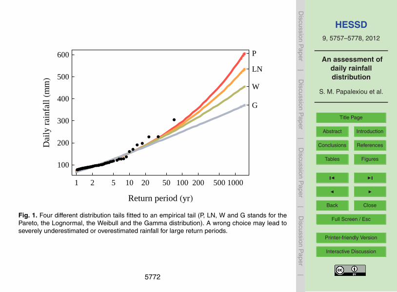
less a very large sample is available), all fitting methods will be “biased” against thetail, since the estimated fitting parameters will point towards the distribution that bestdescribes the largest portion of the data (by definition not belonging to the tail). Clearly,an ill-fitted tail may result in serious errors in terms of extreme event modelling withpotentially severe consequences for hydrological design. For example, in Fig. 1 where20

four different distributions are fitted to the empirical distribution tail, it can be observedthat the predicted magnitude of the 1000-yr event varies significantly.

The distributions can be classified according the asymptotic behaviour of their tailin two general classes, the sub-exponential class with probability densities tending tozero less rapidly than the exponential density, and the hyper-exponential class, with25

densities having tails approaching zero more rapidly than the exponential (Teugels,1975; Kluppelberg, 1989, 1988). Yet, a unique classification does not exist (see e.g. ElAdlouni et al., 2008 and references therein), while many terms have been used in theliterature to refer to tails “heavier” than the exponential, e.g. “heavy tails”, “fat tails”,

5759





HESSD9, 5757–5778, 2012



Title Page



Tables Figures

J I

J I

Back Close

Full Screen / Esc



Discussion

Paper

|D

iscussionP

aper|

Discussion

Paper

|D

iscussionP

aper|

“thick tails”, or, “long tails”, that may lead to some ambiguity: see for example the vari-ous definitions that exist for the class of heavy-tailed distributions discussed by Wernerand Upper (2004). Here, we use the term “heavy tail” in an intuitive and general way,i.e. to refer to tails approaching zero less rapidly than exponential tails.

The practical implication of a heavy tail is that it predicts more frequent larger mag-5

nitude rainfall compared to light tails. Hence, if heavy tails are more suitable for mod-elling extreme events, the usual approach of the adoption of light-tailed models (e.g. theGamma distribution), fitted on the whole sample of empirical data for design purposes(of for example flood protection schemes) would result in a significant underestimationof risk with potential implications for human lives. However, there are significant indica-10

tions that heavy tailed distributions may be more suitable. For example, in a pioneeringstudy Milke (1973) proposed the use the Kappa distribution, a power-type distribution,to describe daily rainfall. Today there are large databases of rainfall records that al-low us to investigate the appropriateness of light or heavy tails for modelling extremeevents. This is the subject in which this paper aims to contribute.15

2 Data

The data used in this study, are daily rainfall records from the Global Historical Climatol-ogy Network-Daily database (version 2.60, www.ncdc.noaa.gov/oa/climate/ghcn-daily)which includes data recorded at over 40 000 stations worldwide. Many of these records,however, are too short in length, have many missing data, or, contain data suspect in20

terms of quality (for details regarding the quality flags refer to the Network’s websiteabove).

Thus, only records fulfilling the following criteria were selected for the analysis: (a)record length greater or equal than 50 yr, (b) missing data less than 20 % and, (c)data assigned with “quality flags” less than 0.1 %. Among the several different quality25

flags assigned to measurements, we screened against two: values with quality flags “G”(failed gap check) or “X” (failed bounds check) which are used to flag suspiciously large

5760





www.ncdc.noaa.gov/oa/climate/ghcn-daily

HESSD9, 5757–5778, 2012



Title Page



Tables Figures

J I

J I

Back Close

Full Screen / Esc



Discussion

Paper

|D

iscussionP

aper|

Discussion

Paper

|D

iscussionP

aper|

values, i.e. a sample value that is orders of magnitude larger than the second largervalue in the sample. Whenever such a value existed in the records it was deleted (thishowever occurred in only 594 records in total, and in each of these records typicallyone or two values had to be deleted). Screening with these criteria resulted in 15 137stations.5

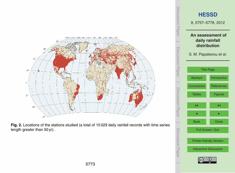
Finally, the statistical procedure, described next, failed to be applied in some sta-tions, for reasons of algorithmic convergence or time limits, resulting in their exclusionfrom the analysis. The final dataset analysed comprises 15 029 stations globally. Thelocations of the stations can be seen in Fig. 2.

3 Methods10

3.1 Statistical approach

The marginal distribution of rainfall, particularly at small time scales like the daily, be-longs to the so-called mixed type distributions, with a discrete part describing the prob-ability of zero rainfall, or the probability dry, and a continuous part expressing the mag-nitude of the non-zero or the wet-day rainfall. As suggested earlier, studying extreme15

rainfall requires focusing on the behaviour of the distribution’s right tail which governsthe frequency and the magnitude of extremes.

If we denote the rainfall with X , and the non-zero rainfall with X |X > 0, then theexceedence probability function (EPF; also known as survival function, complementarydistribution function, or, tail function) of the non-zero rainfall, using common notation,20

is defined as

P (X > x|X > 0) = FX |X>0(x) = 1− FX |X>0(x) (1)

where FX |X>0(x) is any valid probability distribution function chosen to describe non-zero rainfall. It should be clear that the unconditional EPF is easily defined in termsof probability dry p0 as FX (x) = (1−p0) FX |X>0(x). Since we focus on the continuous25

5761





HESSD9, 5757–5778, 2012



Title Page



Tables Figures

J I

J I

Back Close

Full Screen / Esc



Discussion

Paper

|D

iscussionP

aper|

Discussion

Paper

|D

iscussionP

aper|

part of the distribution, and more specifically on the right tail, from this point on, fornotational simplicity we omit the subscript in FX |X>0(x) denoting the conditional EPFfunction simply as F (x). To avoid ambiguity, we clarify that we use the term tail to referonly to the upper part of the EPF, i.e. the part that describes the extremes.

At this point however, we need to define what we consider as the upper part. A com-5

mon practice is to set a lower threshold value xL (see e.g. Cunnane, 1973; Tavaresand Da Silva, 1983; Ben-Zvi, 2009) and study the behaviour for values greater than xL.Yet, there is no universally accepted method to define this lower value. A commonlyaccepted method (known as partial duration series method) is to define the thresholdindirectly based on the empirical distribution, in such a way that the number of values10

above the threshold equals the number of years N of the record (see e.g. Cunnane,1973).

In comparison to the other common method, in which the annual maxima are stud-ied, the method adopted has the advantage of better representing the exact tail of theparent distribution. In contrast, the annual maxima method by selecting the maximum15

value of each year may distort the tail behaviour (e.g. when the three largest daily val-ues occur within a single year, the annual maxima method only takes into account thelargest of them). For this reason, instead of studying the N daily annual maxima, wefocus on the N largest daily values. It is then assumed that these values are represen-tative of the distribution’s tail and can provide information for its behaviour.20

Given that each station has a record of daily values of N years, and a total number nof non-zero values, we define the empirical EPF FN (xi ), conditional on non-zero rainfall,as the empirical probability of exceedence (according to the Weibull plotting position)

FN (xi ) = 1−r(xi )n+1

(2)

where r(xi ) is the rank of the value xi , i.e. the position of xi in the ordered sample25

x(1) ≤ . . . ≤ x(n) of the non-zero values. Thus the empirical tail is determined by the Nlargest non-zero rainfall values of FN (xi ) with n−N +1 ≤ i ≤ n.

5762





HESSD9, 5757–5778, 2012



Title Page



Tables Figures

J I

J I

Back Close

Full Screen / Esc



Discussion

Paper

|D

iscussionP

aper|

Discussion

Paper

|D

iscussionP

aper|

We then fit and compare the performance of different theoretical distribution tails tothe empirical tails estimated from the daily rainfall records previously described. Thetheoretical tails are fitted to the empirical ones by minimizing numerically a modifiedmean square error (MSE) norm defined as

MSE =1N

n∑i=n−N+1

[F (xi )

FN (xi )−1

]2

. (3)5

The need for this modified MSE arises from the fact that in the classical MSE norm,in which the error depends on the difference between the theoretical and the empiricalvalues, i.e. SE =

[F (xi )− FN (xi )

]2, the contribution in the sum of the most important

values for our analysis (those with smallest F (xi )) is too small. On the contrary, thenorm given in Eq. (3) treats each data point equally as it considers the relative error10

between the theoretical and the empirical values which is independent of the absolutevalues. Obviously, the best fitted tail for a specific record is considered to be the onewith the smallest MSE.

The proposed approach, which fits the theoretical distribution only to the N largerpoints of each dataset, ensures that the fitted distribution provides the best possible15

description of the tail and is not affected by lower values. As an example of the fittingmethod, Fig. 3 depicts the Weibull distribution fitted to an empirical sample (the stationwas randomly selected and has code IN00121070) by minimizing the norm given byEq. (3) in two ways, (a) in all the points of the empirical distribution and (b) in only thelargest N points. It is clear that the first approach (dashed line) does not adequately20

describe the tail.It is noted that several other methods have been used extensively in extreme value

estimation, to estimate the parameters of candidate distributions, e.g. the lognormalmaximum likelihood and the log-probability plot regression (Kroll and Stedinger, 1996)and, more recently log partial probability weighted moments and partial L-moments25

(Wang, 1996; Bhattarai, 2004; Moisello, 2007). Yet, the advantage is that the tails fit-ted by the method proposed here can be directly compared since the resulting MSE

5763





HESSD9, 5757–5778, 2012



Title Page



Tables Figures

J I

J I

Back Close

Full Screen / Esc



Discussion

Paper

|D

iscussionP

aper|

Discussion

Paper

|D

iscussionP

aper|

can clearly indicate the best fitted, while in the afore-mentioned methods an additionalmeasure has to be estimated in order to compare the performance of the fitted distri-butions.

3.2 Statistical approach

In this study we estimate the performance of four different common tail types, the5

Pareto, the Lognormal, the Weibull and, the Gamma tails, whose asymptotic behaviourmay be similar with many other distributions. The Pareto and the Lognormal distribu-tions belong to the sub-exponential class and are considered heavy-tailed distributions.The Weibull and the Gamma distribution, depending on the values of the shape param-eter can belong to both classes, but in general their tails are lighter than the Pareto or10

the Lognormal.Specifically, the Pareto type II distribution is the simplest power-type distribution de-

fined in [0,∞). Its EPF is given by

F (x) =(

1+γxβ

)− 1γ

(4)

and it is defined by the scale parameter β > 0, and the shape parameter γ ≥ 0 that15

controls the asymptotic behaviour of the tail, e.g. as the value of γ increases the tailbecomes heavier and consequently extreme values are assumed to occur more fre-quent. For γ→∞ it degenerates to the exponential tail while for γ ≥ 0.5 the distributionhas infinite variance. Many other power-type distributions are tail-equivalent, i.e. ex-

hibiting asymptotic behaviour similar to x−1/γ with the Pareto type II tail, e.g. the Burr20

type XII (Tadikamalla, 1980) the two- and three-parameter Kappa (Mielke, 1973) theLog-Logistic (e.g. Ahmad et al., 1988) or the Generalized Beta of the second kind(Mielke and Johnson, 1974).

5764





HESSD9, 5757–5778, 2012



Title Page



Tables Figures

J I

J I

Back Close

Full Screen / Esc



Discussion

Paper

|D

iscussionP

aper|

Discussion

Paper

|D

iscussionP

aper|

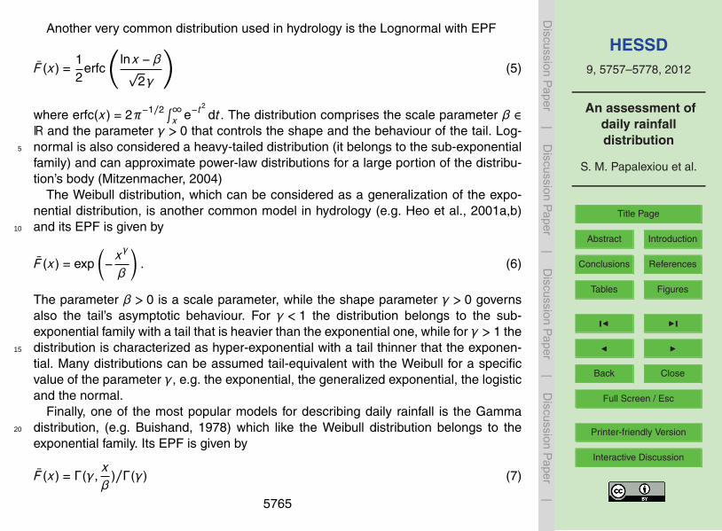
Another very common distribution used in hydrology is the Lognormal with EPF

F (x) =12

erfc

(lnx−β√

2γ

)(5)

where erfc(x) = 2π−1/2 ∫∞x e−t2

dt. The distribution comprises the scale parameter β ∈R and the parameter γ > 0 that controls the shape and the behaviour of the tail. Log-normal is also considered a heavy-tailed distribution (it belongs to the sub-exponential5

family) and can approximate power-law distributions for a large portion of the distribu-tion’s body (Mitzenmacher, 2004)

The Weibull distribution, which can be considered as a generalization of the expo-nential distribution, is another common model in hydrology (e.g. Heo et al., 2001a,b)and its EPF is given by10

F (x) = exp(−xγ

β

). (6)

The parameter β > 0 is a scale parameter, while the shape parameter γ > 0 governsalso the tail’s asymptotic behaviour. For γ < 1 the distribution belongs to the sub-exponential family with a tail that is heavier than the exponential one, while for γ > 1 thedistribution is characterized as hyper-exponential with a tail thinner that the exponen-15

tial. Many distributions can be assumed tail-equivalent with the Weibull for a specificvalue of the parameter γ, e.g. the exponential, the generalized exponential, the logisticand the normal.

Finally, one of the most popular models for describing daily rainfall is the Gammadistribution, (e.g. Buishand, 1978) which like the Weibull distribution belongs to the20

exponential family. Its EPF is given by

F (x) = Γ(γ,xβ

)/Γ(γ) (7)

5765





HESSD9, 5757–5778, 2012



Title Page



Tables Figures

J I

J I

Back Close

Full Screen / Esc



Discussion

Paper

|D

iscussionP

aper|

Discussion

Paper

|D

iscussionP

aper|

with Γ(s,x) =∫∞x ts−1 e−t dt and Γ(s) =

∫∞0 ts−1 e−t dt. Generally, we can assume that

the Gamma tail behaves similar to the exponential tail. Yet, this is only approximatelycorrect as the exponential tail is not asymptotically equivalent with the Gamma tail,i.e. its precise asymptotic behaviour of the right tail depends on the value of the pa-rameter γ, so, for γ > 1 the distribution is sub-exponential and form and for γ < 1 hyper5

exponential.

4 Results

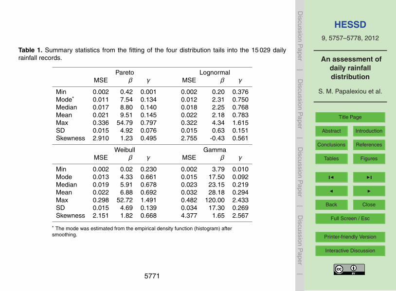
We fit the four previously given distribution tails, following the methodology described,to 15 029 daily rainfall records. The basic statistical results from the fitting are given inTable 1. In order to assess which tail has the best fit, the four tails were compared in10

couples in terms of the resulting MSE, i.e. the tail with the smaller MSE is consideredbetter fitted. As shown in Fig. 4, the Pareto tail was better fitted in approximately morethan 60 % of the stations. Interestingly, the distribution with the heavier tail of eachcouple, in all cases, was better fitted in a higher percentage of the stations, whichimplies a rule of thumb of the type “the heavier, the better”!15

Another comparison revealing the overall performance of the fitted tails was un-dertaken in terms of their average rank. That is, the fitted tails in each record wereranked according to their MSE, i.e. the tail with the smaller MSE was ranked as 1 andthe one with the largest as 4. Figure 5 depicts the average rank of each tail for allstations. Again, the Pareto performed best, while the most popular model for rainfall,20

the Gamma distribution, performed the worst. The percentages of best fit distributiontails are: 30.7 % for Pareto, 29.8 %, for Lognormal, 13.6 % for Weibull and 25.8 % forGamma. Again the Pareto distribution is best according to these percentages; interest-ingly however, the Gamma distribution has a relatively high percentage, higher than theWeibull. This does not contradict the conclusion derived by the average rank. The ex-25

planation is that the Gamma distribution was ranked as best in some cases, but whenit was not best, it was probably the worst.

5766





HESSD9, 5757–5778, 2012



Title Page



Tables Figures

J I

J I

Back Close

Full Screen / Esc



Discussion

Paper

|D

iscussionP

aper|

Discussion

Paper

|D

iscussionP

aper|

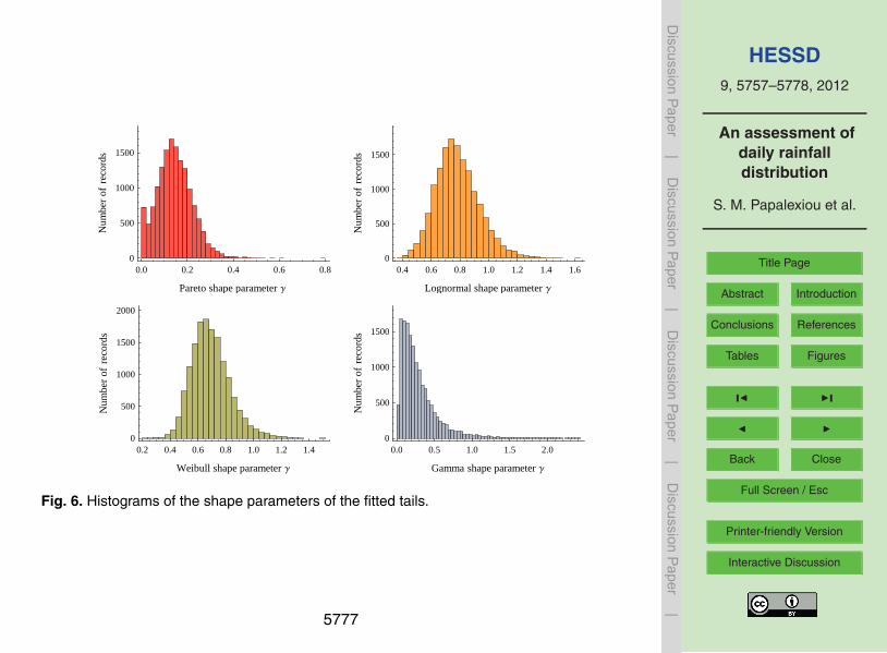
Figure 6 depicts the empirical distributions of the shape parameters of the fitted tails.It is well-known that the most probable values are the ones around the mode, whichfor the Pareto shape parameter is 0.134. Interestingly, this value is close to the onedetermined in a different context by Koutsoyiannis (1999), using Hershfield’s (1961),data set. This implies that power-type distributions, which asymptotically behave like5

the Pareto, will not have finite power moments of order greater than 1/0.134 ≈ 7.5.Moreover, as the empirical distribution of the Pareto shape parameter in Fig. 6 attests,values around 0.2 are also common, implying non-existence of moments greater thanthe fifth order. We should thus bear in mind that sample moments of that or higherorder (sometimes appearing in research papers) may not exist. Regarding the Weibull10

tail, the estimated mode of its shape parameter is 0.661, implying a much heavier tailcompared to the exponential one. Finally, it is worth noting that the estimated modeof the Gamma shape parameter is as low as 0.092. The shape parameter of Gammacontrols mainly the behaviour of the left tail, resulting in J- or bell-shaped densities(loosely speaking, the right tail is dominated by the exponential function and thus be-15

haves like an exponential tail), and a value that low corresponds to an extraordinarilyJ-shaped density that would be unrealistic for describing the whole distribution bodyof daily rainfall. In other words, a Gamma distribution fitted to the whole set of pointswould most probably underestimate the behaviour of extremes.

Finally, we searched for the existence of any geographical patterns, potentially defin-20

ing climatic zones, in the best fitted tails, i.e. the existence of zones in the world wherethe majority of the records were better described by one of the studied distributiontails. The maps in Fig. 7, that depict the station locations where each distribution tailwas best fitted, did not unveil any regular patterns in terms of the best fitted distributionbut rather seem to follow a random variation.25

5767





HESSD9, 5757–5778, 2012



Title Page



Tables Figures

J I

J I

Back Close

Full Screen / Esc



Discussion

Paper

|D

iscussionP

aper|

Discussion

Paper

|D

iscussionP

aper|

5 Summary and conclusions

Daily rainfall records from 15 029 stations are used to investigate the performance offour common tails that correspond to the Pareto, the Weibull, the Log-Normal and theGamma distributions. These theoretical tails were fitted to the empirical tails of therecords and their ability to capture adequately the behaviour of extreme events was5

quantified by comparing the resulting MSE. The ranking from best to worst in termsof their performance is: (a) the Pareto, (b) the Lognormal, (c) the Weibull, and (d) theGamma distributions. The analysis suggests that heavier-tailed distributions in generalperformed better than their lighter-tailed counterparts. It is instructive that the mostpopular model used in practice, the Gamma distribution, performed the worst, revealing10

that the use if this distribution underestimates the frequency and magnitude of extremeevents.

Additionally, we note that heavy tails tend to be hidden (see e.g. Koutsoyiannis,2004a,b) especially when the sample size is small. Thus, we believe that even in thecases where the Gamma tail performed well, the true underlying distribution tail may15

be heavier. This leads to the recommendation that heavy-tailed distributions are prefer-able as a means to model extreme rainfall events worldwide. We also note, that the tailsstudied here are as simple as possible, i.e. only one shape parameter controls theirasymptotic behaviour. Yet, there are many distributions with more shape parametersthan one that may affect the tail behaviour, e.g. the Generalized Gamma distribution20

(Stacy, 1962). Particularly, the Generalized Gamma (a non-power type distribution)and the Burr type XII distributions were compared as candidates for the daily rainfall(based on L-moments) in an earlier study, using thousands of empirical daily recordsand the former performed better (Papalexiou and Koutsoyiannis, 2011).

The key implication of this analysis is that the frequency and the magnitude of ex-25

treme events have generally been underestimated in the past. Engineering practiceneeds to acknowledge that extreme events are not as rare as we had thought – andshift to heavy-tailed distributions for their analysis.

5768





HESSD9, 5757–5778, 2012



Title Page



Tables Figures

J I

J I

Back Close

Full Screen / Esc



Discussion

Paper

|D

iscussionP

aper|

Discussion

Paper

|D

iscussionP

aper|

References

Ahmad, M. I., Sinclair, C. D., and Werritty, A.: Log-logistic flood frequency analysis, J. Hydrol.,98, 205–224, 1988.

Ben-Zvi, A.: Rainfall intensity-duration-frequency relationships derived from large partial dura-tion series, J. Hydrol., 367, 104–114, 2009.5

Bhattarai, K. P.: Partial L-moments for the analysis of censored flood samples, Hydrolog. Sci.J., 49, 855–868, 2004.

Buishand, T. A.: Some remarks on the use of daily rainfall models, J. Hydrol., 36, 295–308,1978.

Cunnane, C.: A particular comparison of annual maxima and partial duration series methods10

of flood frequency prediction, J. Hydrol., 18, 257–271, 1973.European Commission: Directive 2007/60/EC of the European Parliament and of the Council

of 23 October 2007 on the assessment and management of flood risks, Official Journal ofthe European Communities, L 288, 6 November 2007, p. 27, 2007.

Heo, J. H., Boes, D. C., and Salas, J. D.: Regional flood frequency analysis based on a Weibull15

model: Part 1. Estimation and asymptotic variances, J. Hydrol., 242, 157–170, 2001a.Heo, J. H., Salas, J. D., and Boes, D. C.: Regional flood frequency analysis based on a Weibull

model: Part 2. Simulations and applications, J. Hydrol., 242, 171–182, 2001b.Hershfield, D. M.: Estimating the probable maximum precipitation, Proc. ASCE, J. Hydraul. Div.,

87, 99–106, 1961.20

Kluppelberg, C.: Subexponential distributions and integrated tails, J. Appl. Probab., 25, 132–141, 1988.

Kluppelberg, C.: Subexponential distributions and characterizations of related classes, Probab.Theory Rel., 82, 259–269, 1989.

Koutsoyiannis, D.: A probabilistic view of Hershfield’s method for estimating probable maximum25

precipitation, Water Resour. Res., 35, 1313–1322, 1999.Koutsoyiannis, D.: Statistics of extremes and estimation of extreme rainfall, 1, Theoretical in-

vestigation, Hydrolog. Sci. J., 49, 575–590, 2004a.Koutsoyiannis, D.: Statistics of extremes and estimation of extreme rainfall, 2, Empirical inves-

tigation of long rainfall records, Hydrolog. Sci. J., 49, 591–610, 2004b.30

Kroll, C. N. and Stedinger, J. R.: Estimation of moments and quantiles using censored data,Water Resour. Res., 32, 1005–1012, 1996.

5769





HESSD9, 5757–5778, 2012



Title Page



Tables Figures

J I

J I

Back Close

Full Screen / Esc



Discussion

Paper

|D

iscussionP

aper|

Discussion

Paper

|D

iscussionP

aper|

Mielke, P. W.: Another family of distributions for describing and analyzing precipitation data, J.Appl. Meteorol., 12, 275–280, 1973.

Mielke Jr., P. W. and Johnson, E. S.: Some generalized beta distributions of the second kindhaving desirable application features in hydrology and meteorology, Water Resour. Res., 10,223–226, 1974.5

Mitzenmacher, M.: A brief history of generative models for power law and lognormal distribu-tions, Internet Math., 1, 226–251, 2004.

Moisello, U.: On the use of partial probability weighted moments in the analysis of hydrologicalextremes, Hydrol. Process., 21, 1265–1279, 2007.

Papalexiou, S. M. and Koutsoyiannis, D.: Entropy based derivation of probability distributions:10

a case study to daily rainfall, Adv. Water Resour., doi:10.1016/j.advwatres.2011.11.007, inpress, 2011.

Stacy, E. W.: A Generalization of the Gamma distribution, Ann. Math. Stat., 33, 1187–1192,1962.

Tadikamalla, P. R.: A Look at the burr and related distributions, Int. Stat. Rev., 48, 337–344,15

1980.Tavares, L. V. and Da Silva, J. E.: Partial duration series method revisited, J. Hydrol., 64, 1–14,

1983.Teugels, J.: Class of subexponential distributions, Ann. Probab., 3, 1000–1011, 1975.Wang, Q. J.: Using partial probability weighted moments to fit the extreme value distributions20

to censored samples, Water Resour. Res., 32, 1767–1771, 1996.Werner, T. and Upper, C.: Time variation in the tail behavior of Bund future returns, J. Futures

Markets, 24, 387–398, 2004.

5770





http://dx.doi.org/10.1016/j.advwatres.2011.11.007

HESSD9, 5757–5778, 2012



Title Page



Tables Figures

J I

J I

Back Close

Full Screen / Esc



Discussion

Paper

|D

iscussionP

aper|

Discussion

Paper

|D

iscussionP

aper|

Table 1. Summary statistics from the fitting of the four distribution tails into the 15 029 dailyrainfall records.

Pareto LognormalMSE β γ MSE β γ

Min 0.002 0.42 0.001 0.002 0.20 0.376Mode∗ 0.011 7.54 0.134 0.012 2.31 0.750Median 0.017 8.80 0.140 0.018 2.25 0.768Mean 0.021 9.51 0.145 0.022 2.18 0.783Max 0.336 54.79 0.797 0.322 4.34 1.615SD 0.015 4.92 0.076 0.015 0.63 0.151Skewness 2.910 1.23 0.495 2.755 -0.43 0.561

Weibull GammaMSE β γ MSE β γ

Min 0.002 0.02 0.230 0.002 3.79 0.010Mode 0.013 4.33 0.661 0.015 17.50 0.092Median 0.019 5.91 0.678 0.023 23.15 0.219Mean 0.022 6.88 0.692 0.032 28.18 0.294Max 0.298 52.72 1.491 0.482 120.00 2.433SD 0.015 4.69 0.139 0.034 17.30 0.269Skewness 2.151 1.82 0.668 4.377 1.65 2.567

∗ The mode was estimated from the empirical density function (histogram) aftersmoothing.

5771





HESSD9, 5757–5778, 2012



Title Page



Tables Figures

J I

J I

Back Close

Full Screen / Esc



Discussion

Paper

|D

iscussionP

aper|

Discussion

Paper

|D

iscussionP

aper|

1 2 5 10 20 50 100 200 500 1000

100

200

300

400

500

600 P

LN

W

G

Return period HyrL

Dai

lyra

infa

llHm

mL

Fig. 1. Four different distribution tails fitted to an empirical tail (P, LN, W and G stands for thePareto, the Lognormal, the Weibull and the Gamma distribution). A wrong choice may lead toseverely underestimated or overestimated rainfall for large return periods.

5772





HESSD9, 5757–5778, 2012



Title Page



Tables Figures

J I

J I

Back Close

Full Screen / Esc



Discussion

Paper

|D

iscussionP

aper|

Discussion

Paper

|D

iscussionP

aper|

Fig. 2. Locations of the stations studied (a total of 15 029 daily rainfall records with time serieslength greater than 50 yr).

5773





HESSD9, 5757–5778, 2012



Title Page



Tables Figures

J I

J I

Back Close

Full Screen / Esc



Discussion

Paper

|D

iscussionP

aper|

Discussion

Paper

|D

iscussionP

aper|

1 2 5 10 20 50 100 200 50010-5

10-4

10-3

10-2

10-1

1

Daily rainfall HmmL

Exc

eede

nce

prob

abili

ty

Fig. 3. Explanatory diagram of the fitting approach followed. The dashed line depicts a Weibulldistribution fitted to the whole empirical distribution points while the solid line depicts the distri-bution fitted only to the tail points.

5774





HESSD9, 5757–5778, 2012



Title Page



Tables Figures

J I

J I

Back Close

Full Screen / Esc



Discussion

Paper

|D

iscussionP

aper|

Discussion

Paper

|D

iscussionP

aper|

Pareto

60%

Lognormal

40%

Pareto

vs.

Lognormal

Pareto

59%

Weibull

41%

Pareto

vs.

Weibull

Pareto

67%

Gamma

33%

Pareto

vs.

Gamma

Lognormal

58%

Weibull

42%

Lognormal

vs.

Weibull

Lognormal

66%

Gamma

34%

Lognormal

vs.

Gamma

Weibull

73%

Gamma

27%

Weibull

vs.

Gamma

0

20

40

60

80

100

Perc

enta

geof

reco

rds

wit

hbe

tter

fitH%

L

Fig. 4. Comparison of the fitted tails in couples in terms of the resulting MSE. The heavier tailof each couple is better fitted to the empirical points in a higher percentage of the records.

5775





HESSD9, 5757–5778, 2012



Title Page



Tables Figures

J I

J I

Back Close

Full Screen / Esc



Discussion

Paper

|D

iscussionP

aper|

Discussion

Paper

|D

iscussionP

aper|

2.14

Pareto

2.36

Lognormal

2.44

Weibull

3.06

Gamma0.0

0.5

1.0

1.5

2.0

2.5

3.0

Ave

rage

rank

Fig. 5. Mean ranks of the tails for all records. The best-fitted tail was ranked as 1 while theworst-fitted as 4. A lower average rank indicates a better performance.

5776





HESSD9, 5757–5778, 2012



Title Page



Tables Figures

J I

J I

Back Close

Full Screen / Esc



Discussion

Paper

|D

iscussionP

aper|

Discussion

Paper

|D

iscussionP

aper|

0.0 0.2 0.4 0.6 0.80

500

1000

1500

Pareto shape parameter Γ

Num

ber

ofre

cord

s

0.4 0.6 0.8 1.0 1.2 1.4 1.60

500

1000

1500

Lognormal shape parameter Γ

Num

ber

ofre

cord

s

0.2 0.4 0.6 0.8 1.0 1.2 1.40

500

1000

1500

2000

Weibull shape parameter Γ

Num

ber

ofre

cord

s

0.0 0.5 1.0 1.5 2.00

500

1000

1500

Gamma shape parameter Γ

Num

ber

ofre

cord

s

Fig. 6. Histograms of the shape parameters of the fitted tails.

5777





HESSD9, 5757–5778, 2012



Title Page



Tables Figures

J I

J I

Back Close

Full Screen / Esc



Discussion

Paper

|D

iscussionP

aper|

Discussion

Paper

|D

iscussionP

aper|

Fig. 7. Geographical depiction of stations where the best fitted tail is (a) Pareto, in 4621, (b)Lognormal, in 4486, (c) Weibull, in 2051 and, (d) Gamma, in 3871.

5778





an assessment of daily rainfall distribution - hessd

Documents