an assessment of hallux valgus -...
TRANSCRIPT

AN ASSESSMENT OF HALLUX VALGUS
by
Bradley Campbell
B.S. Mechanical Engineering, Tennessee State University, 2006
M.S. Mechanical Engineering, University of Michigan, 2008
Submitted to the Graduate Faculty of
Swanson School of Engineering in partial fulfillment
of the requirements for the degree of
Doctor of Philosophy
University of Pittsburgh
2017

ii
UNIVERSITY OF PITTSBURGH
SWANSON SCHOOL OF ENGINEERING
This dissertation was presented
by
Bradley Campbell
It was defended on
April 4, 2017
and approved by
Patrick Smolinski, PhD, Associate Professor
Department of Mechanical Engineering and Material Science
Qing-Ming Wang, PhD, Associate Professor
Department of Mechanical Engineering and Material Science
Steven Abramowitch, PhD, Associate Professor
Department of Bioengineering
Dissertation Director: Mark Carl Miller, PhD, Research Associate Professor
Department of Mechanical Engineering and Materials Science

iii
Copyright © by Bradley Campbell
2017

iv
The foot is an essential component for human gait and begins the propagation of forces in the
lower extremity of the body. One of the most common conditions that produce forefoot pain is
hallux valgus (HV). HV alters or restricts normal body kinematics, influences physical mobility
and increases the risk of falling. The root cause of HV has not been fully determined. While the
principal kinematics are known and understood, the etiology still remains unclear. Clinically
standard planar radiographs are employed but cannot accurately capture first metatarsal
pronation, which is known to occur in the onset of hallux valgus. Previous research has also
shown changes occur in bone density near the midfoot of cadavers with hallux valgus. Plantar
pressure models have shown patients with hallux valgus have increased loading at the big toe
and metatarsal head. In this study, we analyzed the forefoot of normal and HV patients to
measure in vivo density and bone orientation. We also developed patient specific three-
dimensional finite element models of the first and second rays of the foot to develop predictions
of stress on the metatarsal in the progression of the HV. We found changes in the density profile
in patients with hallux valgus. We quantified pronation in the first metatarsal and found
differences in the patients with hallux valgus. The pronation reported here is the first true three-
AN ASSESSMENT OF HALLUX VALGUS
Bradley Campbell, PhD
University of Pittsburgh, 2017

v
dimensional measurement of metatarsal rotation due to the hallux valgus deformity. We found
differences in contact forces at the metatarsal head and metatarsal base due to hallux valgus.
This study is the first to report an estimate of pressure at the metatarsal sesamoid interface. We
found increased pressure due to the altered kinematics as a result of HV, which can lead to pain
and erosion at the metatarsal head.

vi
TABLE OF CONTENTS
PREFACE ................................................................................................................................... XV
1.0 INTRODUCTION................................................................................................................ 1
1.1 INTRODUCTION TO HALLUX VALGUS ..................................................... 1
1.1.1 What is hallux valgus? .................................................................................. 1
1.1.2 Incidence/Significance .................................................................................. 4
1.2 RESEARCH QUESTIONS ................................................................................. 4
1.2.1 Specific Aim 1 ................................................................................................ 5
1.2.2 Specific Aim 2 ................................................................................................ 6
2.0 CLINICAL BACKGROUND ON HALLUX VALGUS .................................................. 7
2.1 MOTIVATION .................................................................................................... 7
2.1.1 Associated Factors ........................................................................................ 7
2.1.2 Structure of the anatomy.............................................................................. 8
2.1.3 Radiographic Assessment ........................................................................... 12
2.1.4 Treatment Options ...................................................................................... 17
2.2 THEORIES AND HYPOTHESIS .................................................................... 18
2.2.1 Sesamoid Theories ...................................................................................... 19
2.2.2 Conti Hypothesis ......................................................................................... 19
3.0 WHAT IS MODELING? A LITERATURE REVIEW ................................................. 21

vii
3.1 BACKGROUND ON RELATED MODELING USES .................................. 22
3.1.1 Three-dimensional Model Development ................................................... 22
3.1.2 Review of Modeling Uses ............................................................................ 23
3.2 MODELING THEORY .................................................................................... 26
3.2.1 Elasticity....................................................................................................... 26
3.2.1.1 Strain Displacement Relation ............................................................ 26
3.2.1.2 Equation of equilibrium based on the Newton’s second law. ......... 27
3.2.1.3 Constitutive equation .......................................................................... 28
3.2.1.4 Nonlinear Materials ............................................................................ 30
3.2.2 Aspects of Finite Element Modeling .......................................................... 30
3.2.3 How modeling addresses the issue ............................................................. 31
3.2.3.1 Explanation of the technique ............................................................. 31
3.2.3.2 Loading and Boundary Conditions ................................................... 34
3.2.3.3 Solvers .................................................................................................. 35
4.0 STRUCTURES IN THE FOOT AND THEIR MECHANICS ...................................... 37
4.1 MUSCULOSKELETAL SYSTEM .................................................................. 38
4.1.1 Bone Modeling ............................................................................................. 38
4.1.2 Ligament Modeling ..................................................................................... 43
4.1.3 Cartilage Modeling ..................................................................................... 47
4.1.4 Modeling Nonlinearities ............................................................................. 50
4.2 PREVIOUS MODELS ...................................................................................... 52
4.2.1 Yu Paper (Modeling Joint Pressure) ......................................................... 53
4.2.2 Budhabhatti Paper (1st MTP Paper) ......................................................... 53

viii
4.2.3 Flavin Paper (MTP Head Pressure) .......................................................... 54
4.2.4 Spratley Paper (Springs Ligaments; Clinical Measurement) ................. 55
5.0 METHODOLOGY FOR IMAGING ANALYSES ......................................................... 56
5.1 IMAGING PROJECT APPROACH ............................................................... 57
5.1.1 Simulated Weightbearing Device .............................................................. 57
5.1.2 Imaging ........................................................................................................ 60
5.1.2.1 X-Ray Procedure ................................................................................. 60
5.1.2.2 CT Scan Procedure ............................................................................. 61
5.2 DENSITY READINGS ..................................................................................... 63
5.3 BONE ORIENTATION .................................................................................... 64
5.3.1 Clinical Measurements ............................................................................... 64
5.3.2 Landmark Selection for 3D Measurements .............................................. 65
5.4 STATISTICAL ANALYSIS ............................................................................. 70
5.4.1 Clinical Measurement Analysis ................................................................. 70
5.4.2 Densitometric Analysis ............................................................................... 71
6.0 METHODLOGY FOR FEA MODELING ..................................................................... 72
6.1 MODEL CREATION ........................................................................................ 72
6.1.1 CT to CAD Process ..................................................................................... 73
6.1.2 CAD to FE Process...................................................................................... 76
6.2 MODELING CONDITIONS AND SIMULATIONS ..................................... 84
6.2.1 Boundary Conditions .................................................................................. 84
6.2.2 Data Analysis ............................................................................................... 88
7.0 CLINICAL RESULTS ...................................................................................................... 90

ix
7.1 THREE-DIMENSIONAL MEASUREMENTS .............................................. 90
7.2 DENSITOMETRIC ANALYSIS ...................................................................... 96
8.0 FINITE ELEMENT ANALYSIS RESULTS ................................................................ 103
8.1 METATARSOSESAMOIDAL MODEL....................................................... 103
8.1.1 Metatarsal Head and Sesamoids Contact ............................................... 103
8.1.2 Metatarsal Head and Sesamoids Cartilage von Mises Stress ............... 110
8.1.3 FEA Model Validation .............................................................................. 115
8.2 TARSOMETATARSAL MODEL ................................................................. 116
8.2.1 Metatarsal Base and Cuneiform Contact ............................................... 116
8.2.2 Metatarsal Base and Cuneiform von Mises Stress................................. 118
8.2.3 FEA Model Validation .............................................................................. 123
9.0 DISCUSSION ................................................................................................................... 125
9.1 INFERENCES FROM THE ANGLE MEASUREMENTS RESULTS ..... 125
9.2 INFERENCES FROM THE DENSITY RESULTS ..................................... 129
9.3 INFERENCES OF FEA MODELING RESULTS ....................................... 132
10.0 CONCLUSIONS .............................................................................................................. 139
APPENDIX A ............................................................................................................................ 141
BIBLIOGRAPHY ..................................................................................................................... 149

x
LIST OF TABLES
Table 1. Reported Material Properties for Lumped Cancellous and Cortical Bone. .................... 43
Table 2. Composition of the Articular cartilage, tendons and ligaments [70]. ............................ 45
Table 3. Reported Ligaments Material Properties ........................................................................ 47
Table 4. Reported Cartilage Material Properties .......................................................................... 50
Table 5. Nomenclature for angle measurements in each imaging technique. .............................. 69
Table 6. Material properties for the finite element models. .......................................................... 76
Table 7. Material properties for the finite element models. .......................................................... 77
Table 8. Ligaments of interest in the first and second rays of the forefoot. ................................. 79
Table 9. Description of the FEA models used in the study. ......................................................... 83
Table 10. Validation of the metatarsosesamoidal finite element models. .................................. 116
Table 11. Path line averages of von Mises Stress calculated in cuneiform of normal model. ... 122
Table 12. Path line average of von Mises Stress calculated in the cuneiform of the HV model. 122
Table 13. Validation of the tarsometatarsal models.................................................................... 124

xi
LIST OF FIGURES
Figure 1. Hallux Valgus. (A) Image of a hallux valgus foot. (B). X-ray featuring intermetatarsal
angle. (C) X-ray featuring hallux valgus angle measurement. ....................................... 2
Figure 2. Hallux Valgus Surgical Repairs. (Left) Osteotomy. (B). Arthrodesis. ........................... 3
Figure 3. Anatomical structures of the metatarsophalangeal joint [21]. ....................................... 10
Figure 4. Dorsal (A) and Plantar (B) Foot Anatomy [22]............................................................. 11
Figure 5. CT Scanner Components ............................................................................................... 13
Figure 6. Non-Treatment versus Treatment .................................................................................. 15
Figure 7. Hallux Valgus Interventions after one year [28]. .......................................................... 18
Figure 8. Sample stress and strain diagram. ................................................................................. 28
Figure 9. The structural hierarchy of human bone [49]. ............................................................... 38
Figure 10. Bone types [48]............................................................................................................ 39
Figure 11. Haversian Canal........................................................................................................... 40
Figure 12. Components of the tendon components [48] (Text Figure 1.13). ............................... 44
Figure 13. Mechanical failure plot. ............................................................................................... 46
Figure 14. A normal diarthodial joint [48]................................................................................... 48
Figure 15. Weightbearing CT Device. A. CAD Rendering B. Physical model. ........................... 58
Figure 16. Screw Calibration. ....................................................................................................... 59
Figure 17. Weightbearing device in use with horizontal CT scanner. .......................................... 59
xii
Figure 18. Schematic of an x-ray device. ..................................................................................... 61
Figure 19. Interface for measurements taken on CT in Vitrea. .................................................... 65
Figure 20. Long bone landmarks. ................................................................................................. 66
Figure 21. Illustration of the rotation matrix decomposition. ....................................................... 68
Figure 22. Workflow process to create FEA models from the CT scans. .................................... 73
Figure 23. Mesh convergence study. ............................................................................................ 81
Figure 24. Mesh convergence peaks. ............................................................................................ 82
Figure 25. Boundary conditions of the HV model. ....................................................................... 85
Figure 26. Boundary conditions of the normal model. ................................................................. 85
Figure 27. HV (left) and Normal (right) MTS Model. ................................................................. 86
Figure 28. HV (left) and Normal (right) TMT Model. ................................................................. 86
Figure 29. Loading conditions of the HV model. ......................................................................... 87
Figure 30. Loading conditions of the normal model..................................................................... 87
Figure 31. Pronation of the first phalanx relative to the first metatarsal. ..................................... 91
Figure 32. Pronation of the first phalanx relative to the first metatarsal ...................................... 92
Figure 33. Correlation of the intermetatarsal angle measurement from x-ray versus first
metatarsal pronation angle. ...................................................................................... 93
Figure 34. Comparison of group average angular measurements for each imaging technique. ... 93
Figure 35. Correlation of the imaging techniques. ....................................................................... 95
Figure 36. Mean densities of both HV and normal. ...................................................................... 97
Figure 37. Mean densities of both HV and normal groups. .......................................................... 98
Figure 38. Dorsal and plantar density changes at the metatarsal head, base and cuneiform ........ 99
Figure 39. Medial and lateral density changes at the metatarsal head, base and cuneiform ........ 99
Figure 40. Scatter plot and regression of the density in both HV and normal groups. ............... 101
xiii
Figure 41. Scatter plot and regression of the density in both HV and normal groups. ............... 102
Figure 42. Average contact pressure comparison of the normal (left) and HV (right) models. . 104
Figure 43. Average contact area comparison of the normal (left) and HV (right) models. ........ 105
Figure 44. Average contact force comparison of the normal (left) and HV (right) models. ...... 106
Figure 45. The average contact pressure comparison of the normal (left) and HV (right) models
with modified moduli of elasticity. ........................................................................... 107
Figure 46. The average contact area comparison of the normal (left) and HV (right) models with
modified moduli of elasticity. ................................................................................... 108
Figure 47. The average contact force comparison of the normal (left) and HV (right) models with
modified moduli of elasticity. ................................................................................... 109
Figure 48. Comparison of the peak von Mises stress between the normal and HV foot models at
the sesamoids and metatarsal head. .......................................................................... 111
Figure 49. Peak von Mises stress of the metatarsal head in the HV foot model. ....................... 111
Figure 50. Peak von Mises stress of the sesamoids in the HV foot model. ................................ 112
Figure 51. Peak von Mises stress on the metatarsal head in the normal foot model. ................. 112
Figure 52. Peak von Mises stress on the sesamoids in the normal foot model. .......................... 113
Figure 53. Maximum shear stress in the HV model. .................................................................. 113
Figure 54. Maximum shear stress in the normal model. ............................................................. 114
Figure 55. Peak von-Mises stress distribution at the Metatarsal Head in the HV Model. .......... 114
Figure 56. Peak von Mises stress distribution at the metatarsal head in the normal model. ...... 115
Figure 57. Average contact pressure between the (a) normal and (b) HV models. .................... 117
Figure 58. Average contact force between the (a) Normal and (b) HV models. ........................ 118
Figure 59. Von Mises stress in the cuneiform of the normal foot model. .................................. 119
Figure 60. Von Mises stress in the metatarsal base of the normal foot model. .......................... 120
Figure 61. Von Mises stress in the cuneiform of the HV foot model. ........................................ 120
Figure 62. Von Mises stress in the metatarsal base of the HV foot model. ................................ 121

xiv
Figure 63. Path lines in the cuneiform. ....................................................................................... 123

xv
PREFACE
I would like to acknowledge my loving family and wonderful friends responsible for getting me
to this point in life. Very special thanks to my wife, Eloho Ufomata, MD, and my advisors, Mark
Carl Miller, PhD and Stephen F. Conti, MD, for their patience and contributions to my work.
This dissertation is dedicated to the loving memory of Eng Hui Khor, PhD.

1
1.0 INTRODUCTION
The foot is an essential component for human gait. The foot begins the propagation of forces in
the lower extremity of the body, which continues at the ankle through the knee and to the hips.
Foot problems can alter or restrict normal body kinematics, influence physical mobility and
increase the risk of falling [1, 2]. The forefoot in particular, influences the function of the ankle
and forefoot problems range from injury of small foot bones, like the phalanx, to injury of the
tarsometatarsal, a more rigid part of the foot. The most common conditions that produce forefoot
pain are metatarsal stress fracture, hallux rigidus and hallux valgus [3].
1.1 INTRODUCTION TO HALLUX VALGUS
1.1.1 What is hallux valgus?
Hallux valgus, HV or more generally known as a bunion, is one of the most typical foot
disorders [4]. It is a foot deformity, in which the first metatarsal protrudes from its normal
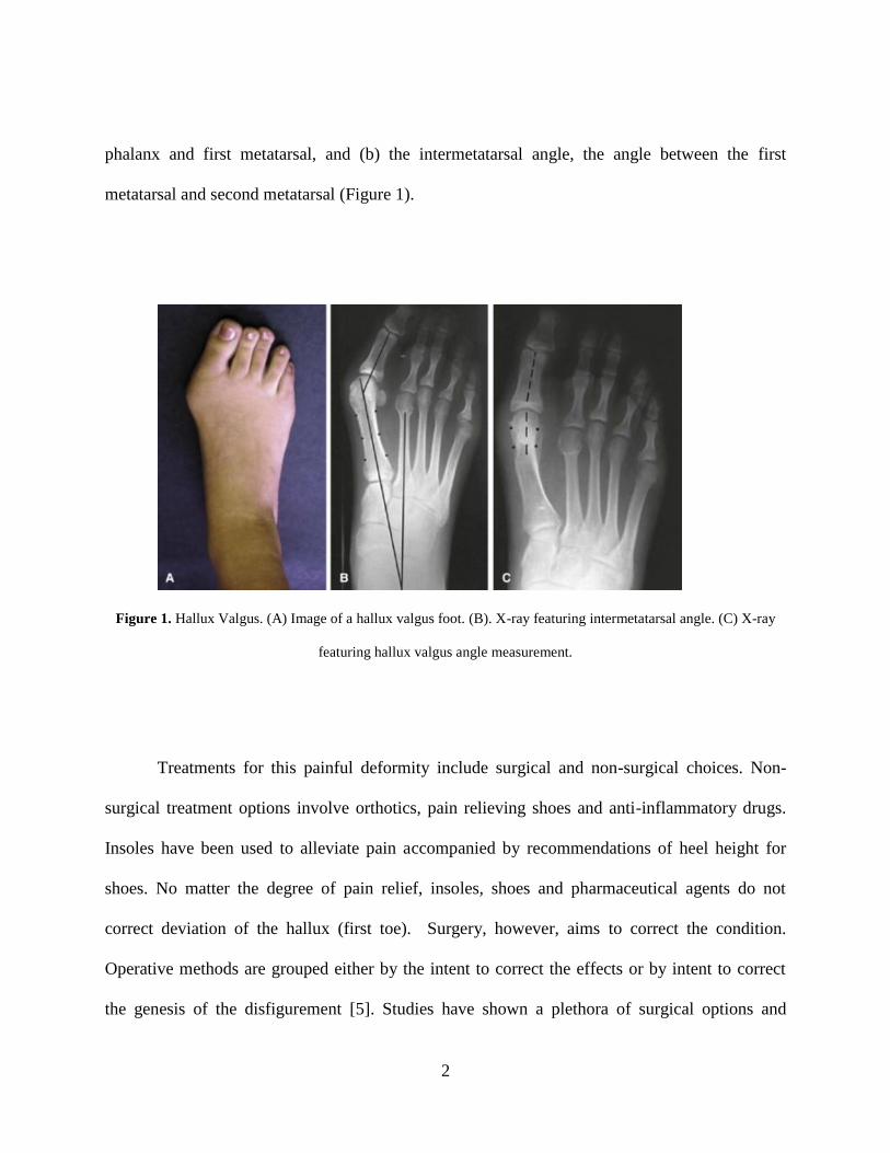
alignment with the hallux (Figure 1). HV has three levels: mild, moderate and severe. Each level
is primarily based on planar angles called the (a) hallux valgus angle, the angle between the first
2
phalanx and first metatarsal, and (b) the intermetatarsal angle, the angle between the first
metatarsal and second metatarsal (Figure 1).
Figure 1. Hallux Valgus. (A) Image of a hallux valgus foot. (B). X-ray featuring intermetatarsal angle. (C) X-ray
featuring hallux valgus angle measurement.
Treatments for this painful deformity include surgical and non-surgical choices. Non-
surgical treatment options involve orthotics, pain relieving shoes and anti-inflammatory drugs.
Insoles have been used to alleviate pain accompanied by recommendations of heel height for
shoes. No matter the degree of pain relief, insoles, shoes and pharmaceutical agents do not
correct deviation of the hallux (first toe). Surgery, however, aims to correct the condition.
Operative methods are grouped either by the intent to correct the effects or by intent to correct
the genesis of the disfigurement [5]. Studies have shown a plethora of surgical options and

3
surgical procedures including osteotomies, arthrodesis and soft tissue procedures (Figure 2)[6].
The initial evaluation is chiefly responsible for the selection of the surgical technique. If
incorrectly evaluated, the treatment of the deformity could lead to revision surgery [7]. In the
United States, approximately 209,000 people undergo HV surgery annually [8]. After surgery,
the incidence of the deformity recurrence may be as high as 16% [9, 10]. A study has found that
of all failed forefoot procedures, first ray surgeries accounted for 66% from a large group of
patients that had previously undergone surgery [11].
Figure 2. Hallux Valgus Surgical Repairs. (Left) Osteotomy. (B). Arthrodesis.

4
1.1.2 Incidence/Significance
Hallux valgus affects females 2.2 - 3.0 times more often than males [4]. The prevalence of hallux
valgus among juveniles, adults and elderly are 7.8%, 23.0% and 35.7% respectively. The cost
associated with the surgeries can be considerable. A very rudimentary bunion surgery costs
roughly $900, a very low estimate, yielding an annual cost of over $180 million dollars. In 2006
in Australia with a population of less than 8% of the United States, the total contribution of
health care in subsidizing surgeon’s fees was $14 million dollars [12]. Given that older patients
have a higher incidence relative to the general population, HV has a meaningful cost to Medicare
[13].
1.2 RESEARCH QUESTIONS
The root cause of HV has not been fully determined. While the principal kinematics are known
and understood, the etiology still remains unclear. As a result, when an intervention addresses a
purported cause, different surgical interventions have different goals. Recent research has shown
changes in bone density near the tarsometatarsal joint with HV in cadaveric specimens [14].
These density changes should be the result of the altered force transmission through the joint
because bone remodels as a function of loading. Measurements of in vivo density changes in
HV patients have not been performed, even though the density changes may directly point to the
causes of HV. Without interventions that address the origin of angular changes, surgeries may
not comprehensively correct the problem of HV.

5
Due to the three dimensional nature of the HV deformity, differences about the origin of
HV, and the lack of data regarding density changes in the metatarsal joints, we have developed a
study to provide the insight necessary for the advancement of medical care of HV. We believe
that the density change in the metatarsal may provide evidence to predict the progression of the
bone that the sesamoid bones play a large role in the occurrence of HV and that first metatarsal
pronation correlates with the severity of the deformity.
The scope of this dissertation is to clinically and mechanically study the first and second
ray of the foot as it related to hallux valgus. The planned investigation takes clinical
measurements related to the deformity and densitometric information to estimate the kinematics
of hallux valgus. The estimated kinematics are then tested in a structural analysis of the foot. The
aims of this study are to extend the understanding of the onset of HV by the following aims:
1.2.1 Specific Aim 1
The first aim is to relate the orientation of the metatarsals and position of the sesamoid with
clinically meaningful angles and determine the density changes in the metatarsal and medial
cuneiform.
(a) In collaboration with the Radiology Department at UPMC, we will recruit and consent
patients that were diagnosed with severe HV and request both non- and weightbearing computed
tomography images.
(b) A three-dimensional computer solid model will be developed from the computed
tomography images. The orientations of the first and second metatarsals, first phalanx and
medial cuneiform will be calculated and statistically compared with clinical HV measures. The

6
three-dimensional rotation of the metatarsal along its own long axis with respect to the whole
foot will be computed and correlated with the intermetatarsal angle.
(c) From the images, numerical assessment of the density of the bone on both sides of the
metatarsal and cuneiform will be conducted (i.e., the bone of interest regarding HV) in the
sagittal (plantar and dorsal) and transverse (medial and lateral) planes. The results will be
compared with existing literature to establish the difference with bone in feet with deformities.
1.2.2 Specific Aim 2
The second aim is to develop a patient specific three-dimensional computational model of the
first and second rays of the foot to develop predictions of the progression of HV deformities and
of the results of surgical interventions. We will:
(a) With the existing three-dimensional solid model, a CAD model will be developed for
use with finite element analysis software.
(b) Conduct static structural analysis of the model with input from known literature
regarding loading of the foot to find contact stresses between joints of the first ray.
(c) Validate the ability of the model’s kinematic output to approximate the foot’s
mechanical behavior. Validation occurs by loading it with bodyweight and comparing the output
configuration’s bone position with a full weightbearing CT imaging of HV patients.

7
2.0 CLINICAL BACKGROUND ON HALLUX VALGUS
2.1 MOTIVATION
HV is three-dimensional problem involving both rotational and oblique displacement changes.
Plain film analysis is typically used in pre-operative planning. These plain films provide insight
into the deformity but do not permit an accurate measurement of the actual varus and rotational
deviations. A true volumetric representation can accurately assess the deformity and resulting
plane projections can be readily derived from a three-dimensional representation. Measurements
of the progression of HV as functions of HV angle and intermetatarsal (IM) angle have used
planar views and have not adequately considered both the three-dimensional configuration and
the planar views. A study that considers three-dimensional and planar views will provide an
improved idea of the progression of disease and improved pre-operative planning.
2.1.1 Associated Factors
Hallux valgus can be congenital or acquired. Congenital hallux valgus deformities are an
inherited birth characteristic and develop without predisposing factors [15]. Patients with
acquired HV develop the deformity over the course of time. Putatively, extrinsic factors related

8
to hallux valgus include weightbearing and footwear. The intrinsic factors for the deformity
include the age and heredity along with other musculoskeletal influences [16].
Certain factors are thought to cause irregular loading within the foot. Pronation of the
hindfoot causes excessive push-off and increased loading directly at the metatarsophalangeal
joint (MTPJ). Pes planus, or flatfoot, a decrease in the arch of the midfoot, causes the
propagation of forces through the foot to impact the tarsometatarsal joint (TMTJ) and MTPJ.
Soft tissue dynamics such as contracture of the Achilles and MTPJ laxity also impact the
deformity’s formation [15].
2.1.2 Structure of the anatomy
The first proximal phalanx, first metatarsal and sesamoid bones comprise the bony tissue
presented during HV diagnosis. The medial cuneiform and second metatarsal are reference bones
included in clinical measurements taken to quantify the scale of the deformity. The sesamoids
are two small bones housed within the tendon of the flexor hallucis brevis and track within the
trochlear surfaces around the crista, a small ridge, on the plantar metatarsal [17]. In general, the
primary function of sesamoid bones is to maintain a sizeable tendon moment arm about the
center of rotation at any joint angle [18]. In a normal foot, the sesamoids track on both the medial
and lateral sides of the plantar metatarsal. They are essential to facilitating load transmission
during the gait cycle and the medial sesamoid has the greater weight bearing responsibility[17] .
Hallux valgus patients are thought to experience pain related to displaced sesamoids rubbing
against the crista. Their absence positively correlates with hallucal functional loss and increased

9
load bearing on the metatarsal head [19]. These compounding factors can adversely impact the
mechanics of the metatarsal.
HV impacts ligaments at three joints of the metatarsal: the MTP, TMT and
metatarsosesamoidal joint (MTS). Collateral ligaments at the MTP joint connect the distal first
metatarsal and proximal first phalanx. The ligaments appear on the medial and lateral sides of
joint. The proximal first metatarsal and distal medial cuneiform form the TMT joint. Ligaments
connect the (1) anterolateral cuneiform and lateral metatarsal, (2) medial surface of the
metatarsal with the dorsal cuneiform and (3) plantar metatarsal and lateral, interior cuneiform.
Ligaments at the MTS joint connect the sesamoids and first metatarsal. The anterior surface of
both the medial and lateral sesamoids is connected to the proximal phalanx by respective
ligaments. The posterior surface of both sesamoids is connected to the first metatarsal by
respective ligaments. The lateral sesamoid is reinforced by having a band that begins at its
posterior surface and extends into the region of the metatarsal near the medial sesamoid
ligaments’ insertion. The two sesamoids are connected by an intersesamoidal ligament.
Involved muscles include the (a) extensor hallucis longus, EHL (b) flexor hallucis longus,
FHL (c) flexor hallucis brevis, FHB (d) abductor hallucis, AbH and (e) adductor hallucis, AdH
(Figure 3). All the muscles synergistically control the function of the big toe, the
flexion/extension of the first phalanx, and adduction/adduction of the big toe [17]. However, in a
foot with hallux valgus, balance of the forefoot musculature becomes compromised [20].

10
Figure 3. Anatomical structures of the metatarsophalangeal joint [21].

11
Figure 4. Dorsal (A) and Plantar (B) Foot Anatomy [22].

12
The development of HV occurs in a series of non-sequential steps. Studies have shown
the first metatarsal pronates in hallux valgus feet yet it is unclear if this predisposes the foot to or
occurs during the onset of hallux valgus [23, 24]. Constriction at the metatarsophalangeal joint
(MTPJ) due to bursal swelling can cause the medial collateral ligaments of the joint to begin to
fail. The proximal phalanx moves into valgus while the metatarsal head drifts medially,
becoming dislocated in a process better known as subluxation. Due to subluxation, the crista of
the metatarsal sits atop the medial sesamoid while the lateral sesamoid drifts into intermetatarsal
space, the region between the first and second metatarsal. As the crista wears away due to its
contact with the sesamoid, the metatarsal head pronates due to forces acting on it [9]. Forces
generated from dysfunctional alignment of the forefoot bones cause abnormal forces along the
metatarsal. These forces cause the phalanx to also pronate [16].
2.1.3 Radiographic Assessment
Hallux valgus is generally described by measurements taken with planar imaging. Plain film
imaging is the process of obtaining two-dimensional radiographs in clinically relevant planes to
observe structures within the body. With respect to the musculoskeletal system, the process can
be full, partial or non-weight bearing for various levels of gradations in the kinematics of the
lower extremity. A three dimensional image can be taken using computed tomography (CT). CT
scans permit cross sectional imaging that is combined to produce a full volumetric representation
of a body part. Commonly obtained horizontally, the standard of care CT for the lower extremity

13
is conducted with the patient on a table prone, supine or perpendicular to the CT gantry.
Obtaining a weightbearing image with CT requires either a vertical scanner with the patient
standing or retrofitting existing horizontal scanners to simulate partial weightbearing.
Figure 5. CT Scanner Components
Clinically, X-ray images are used to view the internal structures of the foot. While the
patient stands on both feet, the X-rays are taken in the anteroposterior (AP) and lateral views. In
the AP view, the HV angle and IM angle are calculated to assess the severity of the deformity.
The hallux valgus angle is an angle measurement between the long axis of the first phalanx and
first metatarsal (Figure 6). The normal HV angle is <15°. Bunion patients, mild moderate and
severe, have a range of 15° - 20°, 21° - 40° and >40° respectively [9] (Coughlin 1996). The

14
intermetatarsal angle is an angle measurement between the long axis of the first and second
metatarsal (Figure 6). The normal IM angle is <9°. Bunion patients, mild moderate and severe,
have a range of 9° - 11°, 12° - 16° and >16° respectively. The sesamoids are assessed in the
coronal view. In normal patients, each sesamoid is seated on a single side of the crista. The
medial sesamoid is beneath the medial epicondyle and the lateral sesamoid is beneath the lateral
epicondyle. The sesamoids are measured on an ordinal scale [19] quantifying the gradation of the
sesamoid location relative to the crista. Grade 0 is normal. Grade 1 describes the lateral side of
the medial sesamoid migrating underneath the crista. Grade 2 describes the medial side of the
medial sesamoid migrating underneath the crista. Grade 3 describes migration of the medial
sesamoid to sit underneath the lateral epicondyle with the lateral sesamoid sitting in the
intermetatarsal space.

15
Figure 6. Non-Treatment versus Treatment
Pronation of the first metatarsal, which occurs in the onset of HV, is not measured
clinically and rarely reported in the literature. Eustace and Collan previously worked on
quantifying the pronation of the first metatarsal in normals and subjects with HV. Eustace
offered a first attempt to measure pronation, yet in plain film x-rays, based on the migration of
the inferior tuberosity in single, combined group of normal, HV and non-HV deformed patients
(n = 100). Eustace further correlated pronation with IM angles measurements in a paired analysis
to find a positive, medium relationship between the two measurements. Work by Collan et al.
improved upon Eustace, by measuring first metatarsal pronation in an HV group with

16
weightbearing CT data. They obtained CT scans of 15 middle-aged subjects in two groups:
controls (n = 5) and those with bilateral HV (n = 10). They reported pronation of the phalanx
and first metatarsal in the coronal plane relative to the ground to be 33 ± 3 and 4 ± 4 in the HV
group and 8 ± 2 and 2 ± 3 in the normal group respectively.
While the utility of CT has been established it is not presently used clinically. Beyond
providing 3D imagery of the anatomy, CT also provides a method for measuring bone density.
Studies to investigate the densitometric profile of hallux can lead to an understanding of the
dynamics that lead to and result from hallux valgus. Densitometric analysis conducted on
normal cadaveric human feet by Muehleman found the head of the first metatarsal to be denser
than the base and the medial region to be the less dense than lateral3. Particularly at the head, the
lateral was denser than the medial. At the tarsometatarsal joint, Coskun et al. divided the sagittal
(lateral, intermediate and medial at the dorsal, intermediate and plantar areas) and transverse
(dorsal, intermediate and plantar at the lateral, intermediate and medial areas) planes into nine
regions. They found that sagittal slices illustrated that the dorsal region of the lateral area in
females was denser than the plantar region and that in transverse slices the lateral areas were
denser than the medial4. Pelt performed a densitometric analysis of cadavers at the cuneiform
and found the plantar, distal region of the medial cuneiform bone was the densest region [25]. A
similar in vivo study in normals by Panchbhavi, found an increase of density in the distal and
dorsal direction of the medial cuneiform [26]. They concluded that the most anterior, dorsal, and
lateral portions of the cuneiform were densest.

17
2.1.4 Treatment Options
Patients suffering from hallux valgus have treatment options to relieve symptoms. While orthosis
can retard the progression of the deformity, research has shown that over time, the reduction in
pain is temporary. One study tracked three groups of bunion patients, two of which underwent
either a surgical or non-surgical intervention, over 12 months. It was found that the third group,
in which no intervention took place, experienced the same pain as the non-surgical group (Figure
7) [27, 28]. The greatest pain reduction over the 12 months’ period was found in the surgical
group. Current surgical techniques return the positions of the phalanx, metatarsals and sesamoids
to their normal alignment through procedures called osteotomy, arthrodesis and arthroplasty. An
osteotomy is the process of cutting and removing sections of bone. An alternative for severe HV
is the arthrodesis, which is process of fusing a joint with orthopaedic hardware in the form of
screws and plates. Arthroplasty is recommended for osteoarthritic, inactive patients. An
arthroplasty is a surgical procedure to realign and/or reconstruct a joint. Most mild deformities
are corrected by osteotomies while the more severe deformities require lateral soft tissue release
along with osteotomy. In general, the soft tissue release is a procedure to divide, cut or release
tendon attachments around first MTP joint [6].

18
Figure 7. Hallux Valgus Interventions after one year [28].
2.2 THEORIES AND HYPOTHESIS
The goal of this work is to perform a comprehensive analysis regarding the orientation and
interaction of the bones in the first and second rays of the foot. Specifically, this study quantifies
how loading impacts the bones and soft tissue of the metatarsosesamoidal joint. The aims of the
study derive from our clinical theories regarding the role of the sesamoids and the impact of
19
loading at the tarsometatarsal joint. Modeling with finite element analysis can capture the
mechanics occurring at the first ray to provide evidence to investigate our theories.
2.2.1 Sesamoid Theories
The literature has general consensus on the role of the sesamoids as weightbearing
structures [29, 30]. It is clear that as the severity of the deformity increases, metatarsal head
pronation and the subluxation of the sesamoids increases [9]. However, it is possible one event
initiates the other. Is sesamoid subluxation a concomitant reaction to the head pronation, or does
the subluxation initiate head rotation? While it has been accepted that soft tissue and crista
failure initiate the subluxation, we believe the role the sesamoids play in pronation of the first
metatarsal head is unclear. The medial sesamoid bears more load than the lateral, but its primary
role is based on its normal position. When reduced to the middle of the metatarsal head, does this
loading condition impact the head and cause pronation? This modeling will provide some insight
into the displacement of the sesamoids and the deviation of the metatarsal.
2.2.2 Conti Hypothesis
The deformity at the TMT is a propagation of the metatarsal deviation due to hallux
valgus. The great toe valgus angulation causes the first metatarsal to drift away in the medial
direction. This bone movement hypothetically causes remodeling and/or incongruency to occur

20
at the joint connection between the proximal metatarsal and medial, medial cuneiform. The (1)
first TMT joint ligaments become incompetent rather which results in varying degrees of
instability. The (2) first TMT joint becomes arthritic over time due to cartilage loss. The (3) first
TMT joint remodels due to increased pressure from medial deviation of the first MT so
radiographically it maintains both congruency and stability. The remodeling can be assessed with
medical imaging. We believe the in vivo density of normal feet differ from HV feet due to the
increased loading demand on the medial side brought on by the change in geometry at the MTP
and TMT joints. The increased loading will appear in the form of larger value of Hounsfield
units, a unit of measurement in densitometric analysis, indicating a relatively denser region of
bone.
The hypotheses will be tested to address the clinical aims of the study. The results from
the densitometric analysis will be used buttress the outcomes of the finite element modeling
which is intended to elucidate the roles of the sesamoids in hallux valgus and hallux valgus
related bone deformities. The strength of the modeling will be reliant on a proper understanding
of the biomechanics and behavior of materials interacting during the onset of the deformity.

21
3.0 WHAT IS MODELING? A LITERATURE REVIEW
Modeling encompasses the processes centered on developing a visual representation of physical
objects within the anatomy for the purpose of analysis. The representations are derived from
medical imaging, three-dimensional in nature and comprise particular aspects or all of the
hierarchy of a physical body. The utility of three-dimensional models includes characterizing
shape, quantifying position and describing kinematics.
Volumetric models can be further extended and inputted as the geometry in finite element
analysis. Finite element analysis (FEA) has previously been put into practice to explore
biomechanical systems. Originally used in more common structural and mechanical systems,
FEA has provided a platform to reconstruct the anatomy of a physiological system, such as the
hip, knee or ankle, for the purpose of mechanical analysis. This type of computational modeling
can be used to better understand the inherent mechanics of different parts of the body and the
implications of surgical interventions.

22
3.1 BACKGROUND ON RELATED MODELING USES
3.1.1 Three-dimensional Model Development
Models of biological systems often originate from medical imaging. Imaging techniques that
provide three-dimensional visualization, such as CT or MRI, are frequently used to create three-
dimensional digital computer aided design representations or “solid models”. The medical
images are often provided in a file format standard known as digital imaging and
communications in medicine (DICOM), which contains identifying headers along with image
pixel data. DICOM files consist of a two dimensional cross-section of the imaged object. During
the physical imaging process, an object is continuously imaged in planes along the length of the
object. A DICOM sequence, a series of all the individual DICOM files, is then created which
represents the full volume. The sequence is then exported in preparation for the next step in the
creation of a three dimensional model.
Segmentation is the next stage in model development and is the process of partitioning
digital images into distinct regions to create a computer-aided design (CAD) file. The DICOM
sequence is imported into a specialized software package to carry out this process. During
segmentation, the series of images of a grouped set is combined, thereby converting the slices
from grouped pixels to a group of voxels, which comprise a volume, e.g. a bone. This process is
repeated until a model for the geometry of interest is completed.
Thereafter is optimization of the model, a process involving surface smoothing and mesh
cleaning to prepare the model for mathematical computational analysis. The importation of an
exported segmentation converts the voxels into a stereolithographic file (STL file). STL files

23
describe a surface by unit normals and vertices. The structures, or surfaces meshes, are created
with vast triangular arrangements. The output from segmentation is usually a set of structures
that are coarse with uneven surfaces. In fully representing a surface, triangles from various
meshes can overlap, leave gaps and be redundant. Eliminating overlapping triangles, filling holes
and smoothing operations can reduce problems encountered in the segmentation process. After
completion, as determined via inspection, the file(s) are exported in a file format better suited for
finite element software. The subsequent file is a solid, fully closed three-dimensional geometric
representation. A common filetype is Initial Graphics Exchange Specifications (IGES). The
exported CAD volumes in the IGES file format, or another accepted format, can be used for
assessing bone kinematics and finite element analysis.
3.1.2 Review of Modeling Uses
Volumetric models of the anatomy are frequently used to determine the relative three-
dimensional position in space of the bones. This method of analysis is more robust and reliable
than standard clinical imaging. The resolution and planar imaging in two dimensional plain film
can distort three dimensional geometry [31]. Obfuscated imaging can make it difficult to view
out of plane positions such as pronation, which occurs in the development of hallux valgus [16,
23, 32]. The three-dimensional calculations of orientation serve as more accurate extensions of
clinical calculations evaluated in a single plane. Several papers report methods quantifying the
orientation of bony structures in the last 30 years. The International Society of Biomechanics
provides a rubric for establishing a coordinate system to determine the orientation of bones in the

24
lower extremity [33] while some authors report novel alternative methodologies. The approach
is twofold: (1) identify bone body based coordinate system and (2) calculate relative orientation.
In the foot, some studies rely on moments of inertia or density based principal axes of
solid bodies to determine body based coordinate systems and others employ unique approaches
based on anatomical landmark selection [34-36] [37]. Researchers have applied landmark-based
analysis, the method of selecting visible specific anatomic landmarks, to determine the
orientation of the whole foot and individual bones that comprise it. Landmark-based analysis
can be employed to calculate a body based coordinate system from a more user-defined
perspective and can incorporate differences in the orientation of bone with and without loading.
Once the body-based coordinate system has been quantified, the relative orientation can be
calculated. Existing methods to calculate the relative orientation of two bones are digital image
registration and rotation matrix decomposition [38]. Each of the methods are published in the
literature and utilized in analyses of forefoot bones.
Authors have published studies that fully quantify bone segments by these
methodologies. In one of the earliest methodological papers, Grood and Suntay introduced a
widely accepted approach that incorporates a sequence specific body based rotations to solve for
3D orientation [39]. More recently, Jenkyn applied this approach in the lower leg and foot [40].
Gutenkunst’s method used landmark based selection and Cardan rotation sequence to find body
based coordinate systems of bones in the whole foot [36]. Yoshioka, measuring the 3D
movement of forefoot bones in response to weight bearing load, compared a group with flatfoot
against a normal control group with digital image registration [41]. They described the
orientation of the metatarsals with Euler angles derived from local coordinate systems attached

25
to the bones. The combinations of methods to define body based coordinate system and calculate
orientation are advantageous techniques to define the kinematics of bone(s).
Researchers have applied similar techniques to understanding the forefoot. Camacho
used moments of inertia for a specific bone to define individual body based coordinate systems
[34]. Ledoux et al used 3D models to compare, quantify and categorize various foot types such
as pes planus and pes cavus [42]. Ledoux et al., using principal axes derived from the density
profile, have calculated Cardan angles quantifying the relative orientation of respective bones
such as the first and second metatarsal. Specific to the a body based coordinate system of the
metatarsal, Mortier reported an analysis of the first metatarsal measuring pronation by choosing
landmarks on the epicondyles of the head while selecting the superior and inferior points at the
base [37]. This methodology provided the foundation for our approach of selecting landmarks
on the metatarsals when calculating the body based coordinate of the bone.
While the methodologies exist to calculate pronation of bone three-dimensionally, only
Ledoux reported rotation of the first metatarsal in non-HV feet. Studies have attempted to assess
pronation of the first metatarsal yet no other study on metatarsal pronation has used volumetric
models derived from three-dimensional weightbearing imaging. Previous studies have consisted
of in vivo imaging with weightbearing devices [38, 43], however, no reported studies incorporate
the technique in assessing 3D bone orientation within an HV patient population. Weightbearing
imaging will be used here to assess the position of bone segments in the foot three
dimensionally.

26
3.2 MODELING THEORY
Solid mechanics is the study of motion and deformation of a continuous mass. Elasticity is the
study of how loading impacts a body’s deformation. The human body represents a continuous
mass with many different materials that behave multiphasically, linearly or nonlinearly and
elastically or plastically. This present work focuses only on materials that behave in a solid,
elastic manner.
3.2.1 Elasticity
The principles of elasticity form the basis for structural analysis. In a structural analysis, the
equations that govern the linear elastic behavior of the body of interest or continua are the:
strain-displacement relationships, equations of equilibrium and the constitutive equations for
elastic material, e.g.., Hooke’s Law. These relationships establish the displacement of material
points from an unloaded state to a loaded state and determine the strains and stresses.
3.2.1.1 Strain Displacement Relation
The strain-displacement relationship is based on infinitesimal strain, which says the deformations
of the body, relative to the dimensions of the body, are small. Axial strain is the change in length
over length and shear strain is the angular change ratio of a shape. More generally, considering
three orthogonal directions, in 3 dimensional coordinates with indicial notation, the relationship
is given as

27
(3-1)
where i,j = 1:3, ε is strain, u is the displacement vector and x is the material coordinate direction.
3.2.1.2 Equation of equilibrium based on the Newton’s second law.
The equations of equilibrium are an expression of the balance of dynamics acting on a body.
This expression considers those physical quantities acting on the interior and exterior of the
body. When a body is deformed, the laws of conservation of momentum and mass must be
obeyed. The strain-displacement relation captures the strain response to the material
displacement vectors. The equilibrium equations capture the stress response of a body to the
material acceleration and force vectors. In terms of stress, the balance of linear momentum is, in
3 dimensional coordinates with indicial notation,
(3-2)
where i,j = 1:3, is stress, is mass density per unit volume, b is the body force and a is the
material acceleration. In cases of static equilibrium, the a term is zero. This is also referred to as
the first equation of motion.

28
3.2.1.3 Constitutive equation
The constitutive model for a linear elastic material is generalized Hooke’s Law. Hooke’s Law
captures the relationship between stress and strain. The modulus of elasticity is a material
property that characterizes the isotropic nature of an elastic material. The shear modulus is a
material property that characterizes the non-collinear behavior of the material with respect to the
orthogonal directions. The relationship can be demonstrated on a plot of a materials behavior on
a stress-strain curve (Figure 8).
Figure 8. Sample stress and strain diagram.

29
The increasing strain linearly increases the stress until a material’s elastic limit is
reached. The linear slope region of the curve is the modulus of elasticity. In indicial notation, the
relationship written as
(3-3)
where i, j, k and l = 1:3, is stress, C is the stiffness tensor and ε is strain. The inverse of the
stiffness tensor is compliance. Stiffness is used to describe the behavior of many materials
including bone and tissue. Orthotropic, linear elastic materials like bone have 3 planes of
material symmetry and 9 independent elastic constants. The stiffness can be described as:
(3-4)

30
where i and j = 1:3, Ei is a modulus of elasticity, Gij is a shear modulus and νij is a Poisson’s
ratio.
3.2.1.4 Nonlinear Materials
Nonlinear analysis, as it relates to FEA in biomechanics analysis, has been used to explore the
behavior of tissue and ligaments that do not act in a linear manner. In general, the mathematical
expressions for nonlinear materials do not assume small deformations. Considering only
orthopedic biomechanics, non-linear governing equations typically account for the large
deformations they undergo. Additionally, because the current work is static, time dependency
will not be considered. The static analysis considers only those structural responses that are
instantaneous with respect to time. The scope of this work will cover contact elements and
modeling and include large deformations.
3.2.2 Aspects of Finite Element Modeling
Finite element analysis (FEA), a numerical analysis technique, is a powerful tool to simulate the
effects forces have on geometry. In mechanics, all aspects of motion, considered as rotation,
translation or deformation, may be considered independently or together.

31
3.2.3 How modeling addresses the issue
In essence, a body can be loaded with a set of forces, subjecting it to varying levels of rotation or
translation, for which the output is the resulting deformation. Wolff’s Law envisioned a
relationship between architecture and the load bearing capabilities of bone [44]. Wolff’s Law
envisioned a relationship between architecture and the load bearing capabilities of bone [44].
However, until modern advances in computing, solving the large number of equations related to
that relationship was difficult. Modeling allows the simulation of specific environments under
various conditions that cannot be reproduced through in vitro or in vivo testing. FEA also allows
the consideration of complex physiological geometries and application of the nonlinear
constitutive behavior of its components. Once assembled with material and structural properties,
models can be tested under different loads in different kinematic configurations.
3.2.3.1 Explanation of the technique
The principles of elasticity are the foundation of FEA. When traction is applied to a body, the
resulting stress and strain are governed by the previously mentioned equations. The displacement
(and by extension the strain, ε) in the system of equations can be solved by (1) analytical and/or
(2) numerical methods. FEA is a numerical solution of the system of equations that represents
the physical quantities and interaction of the bodies of interest.
The equations for finite element analysis can be reduced to a simple form inclusive of
force, stiffness and displacement. It can be written in matrix form as

32
[F] = [K][D] (3-5)
where F is an n x 1 force or moment matrix and D is an n x 1 displacement vector. The
displacement vector variables, ni, are specified by movement at a point in a single degree of
freedom (or more aptly called a finite point). The matrix [K] is the global stiffness matrix that is
comprised of smaller local stiffness matrices. The stiffness between two finite points is described
by each stiffness variable. Once assembled in a global stiffness matrix, the stiffnesses along each
direction in the matrix relates to the stiffness in each direction of the coordinate system used in
the system of equations.
The FEA process involves systematically discretizing an entire body or region of interest
into sections, i.e. finite elements compromised of finite points, to organize the system of
equations for solution. This process is more commonly known as meshing. The accuracy of the
solution is based on the number of sections created and the type of elements used in the
approximation. Each element is comprised of nodes that are grouped together to model a spatial
volume. The elements can be one-dimensional (springs), 2-D (plate or shell) or three-
dimensional (solid). Each element has its own stiffness, which is defined by Hooke’s Law. The
displacement in Hooke’s Law applied to the element is the displacement of the nodes comprising
the element. Individual element stiffness matrices are assembled into the global stiffness matrix.
The scope of this current research study includes one-dimensional elements, which
represent ligaments at the joint connecting bones, and three-dimensional elements, which
represent bone and cartilage. Tension-only springs will alternatively govern some ligament

33
behavior, while tetrahedral and brick elements will be used for meshing the bone and cartilage.
The current study utilizes ANSYS finite element software to conduct the analysis. A list of
element types and descriptions is available in Appendix A.
The FEA process begins only when a CAD structure is meshed. The size of the mesh
dictates the computational expense dedicated to solving the FEA problem. Relatively, small
sized elements comprising a mesh equate to a large number of equations. Because automatic
generators produce mesh patterns that may be poorly shaped, refinement and smoothing
techniques are required so that the pattern is computationally solvable [45]. Simplicity is often a
rule of thumb for mesh generation: begin with a coarsest mesh and refine the mesh as needed.
Areas of high curvature and regions of expected high stress can be reserved for a finer mesh
quality. Measures such as aspect ratio and element length can be used to judge the quality of a
mesh. Aspect ratio is the ratio of an element’s largest and smallest dimensions. Values close to
1 indicate a more uniform shape. Larger values suggest a more elongated shape, which,
depending on the boundary conditions, may lead to erroneous results. Nominally defined, the
element length, with dependency on the element type, can greatly control the size of the entire
mesh [46].
Biomechanical models commonly have irregular geometries. The shapes lack symmetry
and may involve sharp curvature on their surfaces. The element selection for this type of
geometry balances computational expense with reducing complexity. Brick elements, for
instance, may have increased aspect ratios, which escalate the computational expense when used
with non-symmetric shapes. Therefore, more complex meshing alternatives, like tetrahedral
meshes with multiple nodes, may be preferred. Furthermore, mesh uniformity will vary for

34
irregular shapes. Regions of interest, especially those in contact, will have a finer mesh than the
mesh on the remaining regions of geometry.
After discretization and element selection, the next step in building the model is to define
the material properties. In that this study is a static linear structural analysis, the materials will be
modeled as linear, elastic, homogenous and isotropic. The material properties are taken from the
literature where tensile tests were conducted to extrapolate the real time response of bone and
tissue under load. The elastic modulus, Poisson’s ratio and stiffness are the necessary material
properties for the bone, cartilage and ligaments in the model.
3.2.3.2 Loading and Boundary Conditions
In biomechanics, static analysis of motion is simulated by isolating the respective joints and
applying a known or approximated load. These loads are represented with boundary conditions.
The boundary conditions are the constraints in the form of tractions or prescribed displacements
given at the end points or “boundary” of a body. These tractions come in the form of forces,
moments and pressures applied to components within a model. The other constraints relate to the
prescribed displacement, translation and rotation, of components within the model. Applied
element by element, the assignment of boundary conditions describes how bodies are connected
to each other and how they interact with their external surroundings.
There exist six degrees of freedom within a three dimensional coordinate system: 3
translational and 3 rotational. Prescribed motion stipulates which degrees of freedom are
allowable for a given component. Motion can be prescribed or constrained for every level (node,
line, area, single volume, etc.) of an FEA model. When a component is unconstrained, it is free
to move anywhere in space and components that lack enough constraint are subject to rigid body

35
motion. Rigid motion of a body occurs when every particle mass that comprises the component
moves in or about the same direction without deforming. This is undesirable if the intent is to
conduct a static deformation analysis. This unwanted movement could be limited by setting the
displacement or rotation to zero or by applying a load boundary condition.
Once the boundary conditions are in place, the model is complete and the analysis can be
conducted. The outputs from the static structural analysis are typically strain and stress based
measures calculated in element and nodal form. The types of boundary conditions used will have
a direct impact on the solution.
3.2.3.3 Solvers
Different methods exist to solve the set of equations and boundary conditions formulated from
the element methodology. The results are values at the nodes and elements that make up the
mesh. The two types that will be used with this analysis are the direct elimination and iterative
solvers. Both methods relate to inverting the stiffness matrix within equation of motion, but do
so differently.
The direct solver is based on the direct elimination of the equations. The process
involves factorization and storing very large matrices. These matrices are sparse and symmetric
and time much be allocated to rearranging of the rows and columns to shift non-zero elements to
a narrow band along the matrix diagonal [47]. As a result, this robust solution method has a
large memory requirement. This type of solver is recommended for multiple load cases. Within
ANSYS, the direct elimination solver is known as a sparse direct solver. It always produces a
solution if the available memory is sufficient.

36
An iterative solver is another method to solving the FEA problem with a reduced storage
requirement. The iterative solver obtains a solution by successively refining an initial guess to a
solution within an acceptable tolerance. The requirement of factorization does not impact
iterative solvers because matrix-vector multiplication is applied, therefore requiring less
memory. This solver is suitable for large problems but does not guarantee a solution to the
problem therefore the time for resolution could be large. ANSYS offers a variety of iterative
solvers.

37
4.0 STRUCTURES IN THE FOOT AND THEIR MECHANICS
Validation of the model is contingent on the physiological accuracy of materials and replicated
movements and anatomic connections. In this study, musculoskeletal tissues, which have been
well described in the literature, are being modeled whilst experiencing common movements the
bone encounters in the foot during motion. Four tissue types exist in the human body:
connective, epithelial, muscle and nervous. The scope of this effort is to represent only different
forms of connective tissue in a computational foot model.
Connective tissue is a fibrous linkage that supports other tissues and organs within body.
Connective tissue consists of three components: cells and two extracellular matrix (ECM)
constituents, fibers and ground substance. The fibers are composed of proteins: collagen and
elastin. Collagen is a structural protein found in extracellular matrix. There are five types of
fibrous collagen (I, II, III, V and XI) and more than twenty-five known types of collagen overall
[48]. Collagen is found in bone, cartilage, and tendons. It gives bone, ligaments and cartilage
their structures and properties necessary to perform their respective roles in the body. Elastin is
a protein found in tissues giving them restitutive properties after contracting or stretching. The
second constituent of the ECM is the ground substance, which forms an interfibrillar network.
The ground substance is formed by of proteoglycans, glycoprotein polymer chains with high
sugar content, and glycosaminoglycans, a hydrophilic molecule containing modified sugars [48].

38
4.1 MUSCULOSKELETAL SYSTEM
4.1.1 Bone Modeling
Figure 9. The structural hierarchy of human bone [49].
Bone is a living, rigid organ that carries the responsibility of load bearing in the musculoskeletal
system. Bone is composed of supportive, dense tissue. Bone is organic, a Type I collagen with
fluid and blood contents, and inorganic, a solid extracellular matrix comprised of a modified
form of hydroxyapatite also known as bone mineral (Figure 9). The mineral is the lowest level
of bone composed of long and parallel collagen fibrils and gives bone its stiffness. The matrix
bears the responsibility as the scaffolding for bone [48]. Bone is heterogeneous and of two tissue

39
types, cortical and cancellous (Figure 10). Cortical bone is the hard shell on the exterior of a
bone. The endosteum lines its inner surface near the opening or medullary cavity of long bones.
The periosteum is the vascular connective tissue that lines the external surface of bone.
Figure 10. Bone types [48].
Osteons, the main structural unit for cortical bone, are cylindrical structures within the
bone. Osteons consist of concentric structures of lamellae that surround a central hollow known
as the Haversian canal as seen in Figure 11. The less dense inside of a bone is cancellous bone.
The cancellous bone is composed of trabeculae which forms a porous structure that is spongy in
appearance [48]. Bone mineral, the inorganic segment, gives bone its compressive strength. The
bone mineral density is the amount of bone mineral per unit volume, which changes over the
lifespan. Remodeling occurs due to bone’s sensitivity to loading and high level of adaption to
overuse and nonuse. The process is regulated mechanically. The intent of remodeling, which

40
occurs more in cancellous bone, is to replace old tissue with new tissue such that the total
amount of bone remains unchanged during this entire process. Three types of bone cells control
the remodeling of bone: osteoclasts, osteoblasts and osteocytes.
Figure 11. Haversian Canal.
Osteoclasts are involved in the reabsorption of old bone in the matrix. Osteoblasts are
responsible for the production of new bone and its constituents within the matrix [48].
Osteocytes are cells derived from osteoblasts. In their lifespan osteocytes have a role in bone
formation and much later in their life are involved in bone resorption [50]. During the
remodeling process, mononuclear preosteoclasts form multinucleated osteoclasts at the bone

41
surface. Osteoclasts open a cavity to resorb bone for the deposition of new bone mineral.
Precursors to osteoblasts appear near the cavities, proliferating and differentiating into pre-
osteoblasts and eventually mature osteoblasts at the surface of the cavity. Osteoid is then
released at the site forming new bone that has not yet been mineralized. Once mineralized with
calcium and phosphorus, the site is then covered with flattened lining cells and remains dormant
until the next cycle [51]. The disruption of bone’s remodeling processes can lead to low bone
mineral density which can cause osteoporosis, a condition in which bones loses its strength.
Bone shapes are classified as long, flat, short, irregular and sesamoid. The forefoot is
comprised of many long bones. The mechanical response of long bones is dependent on how
they are loaded. In cortical bone, the parallel assembly of osteons establishes the orientation of
the microstructure. The cancellous bone has its anisotropy due to the orientation of the
trabeculae. This dependence on orientation means bone is stronger in compression than tension
and in the longitudinal direction relative to the transverse and shear directions.
In general, the elastic modulus is influenced by the orientation of the bone. Long bone is
strongest mechanically when loaded on its long axis and has higher compressive strength than
tensile strength [52]. The anisotropic mechanical behavior of bone gives rise to an elastic
modulus that varies by mechanical axis. Research has explored the mechanical characteristics of
bone [53]. Mechanical tests by Reilly and Burstein reported the modulus and ultimate stress of
cortical bone as 17.1 GPa and 159 MPa respectively [54]. A review paper by Currey, cites the
advent of micro-CT usage in the development of an FEA model to find mechanical properties by
predicting strains based on the inherent density and applied loading [52]. Taylor used modal
analysis, in vitro and computationally with FE, to find mechanical properties [55]. Long bone is
strongest mechanically when loaded on its long axis and has higher compressive strength than

42
tensile strength [52]. The anisotropic mechanical behavior of bone gives rise to an elastic
modulus that varies by mechanical axis.
Several papers have included both bone types in models as either homogenous or
heterogeneous. The homogenous models lump the material properties for the cortical and
cancellous bone, representing the mechanical behavior with an approximated value for the single
modulus of elasticity and Poisson’s ratio. The heterogeneous models include separate material
properties for both cortical and cancellous bones.
The mechanical properties of bone have been explored through experimental testing.
Nakamura cites 7300 MPa, for homogenous bone, as commonly used as the modulus of elasticity
for bone [56]. The modulus of elasticity for heterogeneous bone has been found to be 17000
MPa and 445 MPa for cortical and cancellous bone respectively. Cortical bone has an apparent
density of 1.85 g/cm3 [18] while the density of cancellous bone is 0.30 g/cm3 – 0.50 g/cm3 [30].
Longitudinal ultimate stress values for cortical and cancellous bone are 193 MPa and 5.3 MPa in
compression [30, 54, 57, 58].
The effect of bone composition on mechanical behavior has been explored with FEA
analysis. Garcia-Aznar studied the differences of modeling with homogenous and heterogeneous
material properties [59]. Data from Nakamura’s experimental work, which is frequently cited by
bone and tissue FEA papers [60-64], was used with the model (Table 1). The heterogeneous
properties of the Garcia-Aznar model originated from work comparing experimental and
computational surgical repairs [65]. The results of Garcia-Aznar‘s composition comparison
showed differences in the principal stress distribution across the surface of the metatarsal, with
values increasing with heterogeneous moduli. But no difference was shown in horizontal and
vertical displacement between the two methods. Trabelsi’s modeling approach used the absolute

43
bone density profile taken from an individual CT scan and extended it to a moduli distribution
that was inhomogenously elastic [66].
Table 1. Reported Material Properties for Lumped Cancellous and Cortical Bone.
Material Young’s Modulus (MPa) Poisson’s Ratio Source
Lumped Bone
7,300 0.30 [56]
10,000 0.34 [67]
4.1.2 Ligament Modeling
Ligaments are dense bundles of collagenous fibers. In general, ligaments connect bones to other
bones creating joints. They constrain the direction of bone motion thus guiding the movement of
joint articulations. Collagen, subfibrils, fibers, subfascicular units, fasiculi and the macroscopic
tissue compose the hierarchy of ligamentous tissue (Figure 12).

44
Figure 12. Components of the tendon components [48] (Text Figure 1.13).
The fibers align with the long axis of the ligament with a complex orientation of fibrils
[30]. The constituents of ligaments are 20% cellular and 80% extracellular [48]. The
extracellular material is one-third solid and two-thirds water giving it viscoelastic properties
(Table 2). The solid constituents are mostly collagen, elastin, proteoglycans and glycolipids
[68]. The dry weight of the ligament is 70% - 80% type 1 collagen, 10% - 15% elastin and 1% -
2% proteoglycans. The ligament is composed of cross-linked collagen molecules that form fibrils
that become fibers. Ligaments gain their strength from this cross-linked structure. The ligaments
of the extremities such as the foot have a smaller amount of elastin. By comparison, elastic
ligaments in other parts of the body have a 2-to-1 ratio of elastin to collagen [48] fibers, such as,
in ligament flavum (spinal ligament) giving it energy storage and return characteristics.
Ligaments do not heal well and damage can lead to the instability of a joint. This is, in part,

45
because during healing, the composition and architecture of the ligament is altered along with the
ability of the collagen crosslink to completely mature. Nonetheless, remodeling does take place
and, depending on the severity of injury and its location, ligaments could regain their original
function [69].
Table 2. Composition of the Articular cartilage, tendons and ligaments [70].
Collagen Proteoglycan Water
Percentage of Dry Weight
Articular Cartilage 50 - 75 15 - 30 58 - 78
Tendon 23 - 30 ≈ 7 ≈ 70
Ligament ≈ 23 ≈ 7 ≈ 70
Ligaments behave nonlinearly and viscoelastically. The ligaments display a stress strain
curve similar to many biological tissues, with an elongated toe region (Figure 13). Collagen
fibrils in ligaments are arranged in a crimped pattern. In the toe region, the collagen begins to
uncrimp as the applied force increases. The linear region is where the collagen crosslinking
becomes stressed and the crimping stretches and slope of the curve represents ligaments’
modulus of elasticity. The failure region is the yield point of the tissue and represents fiber
damage [71].

46
Figure 13. Mechanical failure plot.
Researchers have explored the mechanical properties of foot ligaments, examining [72]
and carrying out biomechanical tests [73] on the connections near the ankle and midfoot. Seigler
et al. extended the work by Attarian et al. on the modulus of ligaments (Table 3) [74]. These
papers all disregarded viscoelastic behavior in the ligaments. Seigler tested the medial
(tibiocalcaneal, tibiospring, posterior tibiotalar and tibionavicular) and lateral (posterior
fibulotalar, fibulocalcaneal and anterior fibulotalar) collateral ankle ligaments. Mkandawire et al.
conducted an extensive dissection of the foot and ankle and reported the morphometric
properties permitting computer-aided replication of the foot and ankle ligaments. Kura reported
data from mechanical testing of the ligaments at the cuneiform [75]. They found the modulus
values for the Lisfranc and dorsal ligaments. Jacobs et al investigated the foot, attempting to
reproduce the articulations during mid-stance for stress analysis [60].

47
Table 3. Reported Ligaments Material Properties
Material Young’s Modulus (MPa) Poisson’s Ratio Stiffness (N/mm) Source
Ligament 260 0.3 - [73]
5.5 - - [75]
- 1500
The values of structural properties, such as stiffness (load-deformation linear curve) of
ligaments have varied in the literature. Earlier stiffness values of the ligament from FEA models
were as high as 1500 N/mm [76]. Others have used approximated values in the range of 100 -
250 N/mm. Its failure levels are 80 -120 MPa. While ligaments exhibit viscoelasticity, the nature
of modeling will dictate the behavior. The application of short duration loads will reduce the
impact of viscoelasticity because time-dependent properties will not be given a sufficient period
to act.
4.1.3 Cartilage Modeling
Cartilage is a structure that covers bone at its interface with other bones. It is a flexible
connective tissue existing in three different forms: elastic cartilage, hyaline cartilage and
fibrocartilage. Articular cartilage is the hyaline cartilage, a type II collagen, found on articular
surfaces, inside the synovial joint cavity of long bones (Figure 14). Synovial fluid in the joint
lubricates the surfaces of bone. The cartilage contains no nerves or blood vessels and its

48
nutrients must be diffused or convected. The surface texture of hyaline cartilage is smooth and
its appearance has a shiny, translucent blue tint [48]. Hyaline cartilage is multiphasic having
solid and fluid components. The tissue constituents are over two thirds water, which represents
65% – 85% of the weight. It is comprised of collagen and ground substance, composed of
proteoglycans and elastin. The role of the collagen is to stretch and the proteoglycans retain
water. Proteoglycans are 5% – 10% the wet weight while the dry weight of hyaline cartilage is
composed of 40% collagen arranged in cross-linked fibers. These collagen-collagen crosslinks
increase the tensile strength and stiffness. Combined they form the extracellular matrix of the
cartilage, which response to the shearing and compression it undergoes. It fails under tensile
loads exceeding 20 MPa and compressive loads of 35 MPa [77].
Figure 14. A normal diarthodial joint [48].
.

49
Articular cartilage is multiphasic, non-linear and viscoelastic and its low coefficient of
friction and shape help distribute loads across the surface of a bone. Water, collagen and
proteoglycans provide the mechanical properties of cartilage. Damage to cartilage, such as
cracks formed by high tensile stress, reduces its resistivity to compressive loads.
The biphasic nature of cartilage allows it to be modeled differently based on the
conditions of loading. Overall cartilage is represented as having solid and fluid phases. Yet
under deformation, interstitial fluid flows through the articular surface of the cartilage. The
response of the cartilage is the response of all its constituents, including but not limited to the
collagen, elastin, proteoglycan, cell and interstitial fluid. During short rapid loading, the fluid
components do not have time to react relative to the solid constituents. Therefore the tissue
behaves as a solid, elastic material [78]. The biphasic response is only realized mechanically,
during longer duration loading events.
FEA papers in the literature have modeled cartilage as elastic, but have also used
viscoelastic models to do so. Some papers have applied more complex hyperelastic models that
govern the mechanical behavior. Considering only the linear elastic approach, mechanical tests
by Athanasiou reported mechanical properties for cartilage. Athanasiou et al. published
Poisson’s ratio, aggregate modulus and thicknesses values for cartilage sites around the
metatarsophalangeal joint [79]. Some papers have [78, 80] cited review work by Mow,
elucidating biphasic mechanical properties which suggested Young’s modulus values in the
elastic phase, ranging between 0.48 - 0.69 MPa [20]. It was found to fail at an average of 35
MPa [77].

50
Table 4. Reported Cartilage Material Properties
Material Young’s Modulus (MPa) Poisson’s Ratio Source
Cartilage 0.45 – 0.80 0.4 [78]
1.39 0.04 - 0.07 [79]
10 0.4 [60]
The mechanical behavior of cartilage can be altered by disease. Osteoarthritis is an
example of a major disorder related to articular cartilage. Osteoarthritis is the breakdown of
cartilage within a joint cavity. When damaged, unlike bone, collagen does not heal and remodel
well. As a result, the cartilage become stiffer, wears away and its ability to transmit forces
becomes diminished which results in more significant harm to excessive loading.
4.1.4 Modeling Nonlinearities
Mechanical tests conducted on biological materials can demonstrate nonlinear behavior. Tissues
exhibit large deformations in their normal physiological behavior. The large deformations
produce shapes in the tissues that are nonlinear and overall this behavior is represented in a
stress-strain relationship. The stress/strain nonlinear data can be fit mathematically to a curve
used to form a constitutive equation, which includes nonlinearities, such as hyperelastic models.
Papers have included hyperelastic models such as Mooney-Rivlin, to represent the behavior of a
particular volume. The hyperelastic models are taken from strain energy functions to describe
51
both ligaments and cartilage. The aforementioned hyperelastic modeling of cartilage has been
conducted with the intent of describing the joint articulations in a more physiologic manner. The
authors’ analyses are more focused on the behavior of soft tissue exclusively and its constraints
on the lesser toes.
Other papers have described nonlinear materials. The nonlinear nature of the ligaments
with spring based, nonlinear models has been reported. These papers model the ligaments as
nonlinear based on force-displacement attributes taken from the “toe” and linear region of stress-
strain plots. While the authors simulated early weightbearing over a brief time period during
stance, the model contained other material simplicities such as rigid bone to limit the
computation expense of modeling nonlinearities. The scope of this current study extends only to
linearity. Our model is deformable and the duration of the applied loading is short, which does
not require nonlinear modeling.
The short duration also impacts the biphasic nature of the tissues. The only phase of
interest is the solid phase. Viscoelasticity will not be represented in the model and nonlinear
materials will not be included. This negates the use of any time dependent mechanical variables.

52
4.2 PREVIOUS MODELS
Finite element analysis has been a robust tool for predictive and descriptive analysis of
biomechanical systems[81]. Researchers have modeled joints at the shoulder [82], elbow [83],
hip [84], knee [85] and foot [64]. These models have been used to examine the force
transmission at the respective areas of the body to elucidate the roles of the bone, muscles and/or
tissues with respect to particular movements. Models have shown the impact of surgical
intervention in a range of studies from dental implants to total ankle replacements. The models
have reported important results such as the strain across a bone, the stress as a result of a contact
between bodies or the loads to cause failure of tissue.
This study will use FEA to analyze the first ray of the foot, investigating the impact of the
sesamoids on the kinematics of the first ray in the formation of hallux valgus and specifically
quantify mechanics related to pronation of the first metatarsal. FEA has already been used to
analyze the ankle, whole foot and interactions of its joints. In particular, the foot has been
explored with several three-dimensional computational models[86]. Models have investigated
the impact of footwear [87], surgical interventions [88], rigid body dynamics for clinical
measurement [89] and pressure on the head of the first metatarsal [90]. Garcia-Aznar contrasted
homogenous and heterogeneous compositions of the by first metatarsal in an FEA model.
Isvilanonda et al. used FEA to quantify the forces of the forefoot muscles during the onset of a
foot deformity. In each study, the models implemented real bony geometry, diverse material
properties and simplified boundary conditions to obtain the kinetic and kinematic response to
mechanical load.

53
Other studies more directly relate to our work. Similar to our aim, they have addressed
the metatarsophalangeal joint attempting to (1) elucidate metatarsal related contact pressures and
(2) demonstrate the ability of computational modeling to serve as a clinical diagnostic tool.
4.2.1 Yu Paper (Modeling Joint Pressure)
Yu et al. explored the effects of high heeled shoes on the foot and ankle. The model consisted of
28 bony segments connected, in most cases, by tension only ligaments with frictionless contact
between the bone and encapsulated soft tissue. The material properties were defined as
homogenous, isotropic linear elastic for the bone and cartilage and the encapsulated soft tissue
was hyperelastic. Specific total mesh/element size information was not reported.
Yu et al. were using the model to simulate standing in a high heel shoe by applying a
muscle force and a bodyweight based reaction force against a surface underneath the foot and
shoe. The upper region von Mises stress of the MTP was reported as 2.83 – 4.46 MPa along with
plantar surface and other joint stress distributions.
4.2.2 Budhabhatti Paper (1st MTP Paper)
Budhabhatti et al. used an FEA model to calculate the pressure at the MTP head during push-off
and corresponding surgical interventions. The metatarsal and sesamoids were grouped together
as a single body in the model and both distal and proximal phalanges were encased by the soft
tissue resting on a floor. The bones were rigidly modeled and soft tissue was incompressible and

54
hyperelastic. The element type was an 8-node hexahedral mesh with various mesh densities the
largest being 10,416 elements.
After aligning a generic foot model to agree with well experimental data, the model was
loaded at the metatarsal base to simulate push off and treatment interventions. They found
barefoot peak pressures 0.60 – 0.95 MPa at the MTP head and 0.50 – 0.80 MPa at the hallux at
push off. Treatment intervention simulations showed a dependency on the dorsiflexion angles
exists to reduce the pressures at the MTPJ. The introduction of insoles reduced pressures at the
MTP. Because the model includes a lumped sesamoid and metatarsal complex, the contact stress
as a result of the sesamoids is not shown.
4.2.3 Flavin Paper (MTP Head Pressure)
Flavin et al. developed a model of the first ray responds to normal and abnormal loading. The
model included bones (proximal phalanx, metatarsal and sesamoids) and soft tissue
representations. The bones and articular cartilage were modeled as homogenous, elastic
isotropic materials. The soft tissues were model as elastic beam structures. The bone mesh was
formed by tetrahedral elements; the muscle as nodal beams and the total mesh included 204,006
elements.
Flavin used six conditions to model the balance and imbalance of the loading. Fixing the
phalanx and sesamoids in place, the metatarsal was rotated to simulate heel rise based on the six
conditions. Normal loading produced peak stress on the cartilage of 3.6 MPa. The medial band of
the plantar fascia was increased 30% that produced peak stress on the cartilage of 7.3 MPa and
6.8 MPa at the metatarsosesamoid joint. Our modeling results will be compared to this output.

55
4.2.4 Spratley Paper (Springs Ligaments; Clinical Measurement)
Spratley conducted a biomechanical analysis of the patients with flatfoot deformity by rigid body
computational modeling. The goal of the paper was to validation the model’s clinical utility. Six
models, with all bones in the foot apart from the phalanges, were developed, constrained with
force ligament tension and active muscular contractions and loaded with body weight. Each of
the models was loaded through the tibial plateau with the patients’ actual weight.
The output for the model was compared with measurements taken through traditional
clinical methods. They reported good agreement between the measurements taken from the
model and the clinical measurements. The found R squared values ranging between 0.174 –
0.885 for the measurements taken. Their unique validation method will be adopted as a rubric for
our model’s validation.
These papers laid a foundation of methods and results comparison for our current work.
Spratley’s paper demonstrated the clinical utility of developing a rigid body model for
investigating foot pathologies. The results from Yu, Budhabhatti and Flavin are comparable to
the results from our MTP head pressure modeling efforts. The next chapter addresses the clinical
and modeling methodology to meet our clinical aims and to compare with the FEA literature.

56
5.0 METHODOLOGY FOR IMAGING ANALYSES
The methodology to achieve our aims will be described, separately, for the clinical and
mechanical aspects of this project. From a clinical standpoint, we used patient CT scans to make
clinically relevant, standard measurements. Mechanically, the HV finite element foot model was
used to further explore the deformities’ impact on the kinetics in the forefoot.
The first aim of the project, a clinical analysis, was to roentgenologically compare the
kinematics and kinetics of the first ray in HV patients against normal controls patients. The
purpose was to relate the orientation of the metatarsals with clinically meaningful measurements
and quantify first metatarsal head pronation. The three dimensional orientation of the bones in
the first ray was determined by calculating the 3D position of individual bones within a single
foot and comparing their relative orientations. The output, three angles representing rotation
about each of the axes, was compared with measurements from planar standard of care images.
A densitometric analysis of the bones of the first ray was also performed with the CT scan in
female HV patients.

57
5.1 IMAGING PROJECT APPROACH
Weightbearing and non-weightbearing measurements were used to explore pronation and
densitometric analysis examined the influence of loading in the metatarsal and cuneiform. The
University of Pittsburgh Institutional Review Board approved all clinical aspects of the research
study.
5.1.1 Simulated Weightbearing Device
HV is a deformity by which the kinematics change with loading [91]. Vertical CT scanners are
available on the market, but can be extremely expensive. Alternatively, retrofitted devices have
been developed and employed for use with CT/MRI devices in research studies [38, 92]. We
developed and built a device for use in a horizontal gantry CT scanner. The main function of the
device was to apply a load to a patient's foot during a CT scan to simulate full weightbearing.
The device allowed variation of the pressure distribution between the heel and forefoot. The
device was comprised of a platen with both a spring-loaded pedal and a seat at an adjustable
distance from the device (Figure 15). The deflection of the springs provided a load on the foot
and ankle. The load to maximum spring deflection was chosen by an adjustment of two limiting
bolts that restrained the spring deflection. The patient's foot pushed on the top, moveable plate
until it compressed the springs and was stopped from further movement by the bolts.

58
A
B
Figure 15. Weightbearing CT Device. A. CAD Rendering B. Physical model.
The pedal and adjustable seat were constructed from 3/4-inch thick Delrin and fastened
with nylon hardware. Both the pedal and seat easily detached for portability. The pedal
mechanism was designed such that the initial load, prior to any movement of the calibration
screw, was 92 N. Based on the patient weight, the load of half body weight (BW) was calculated
and the screw was adjusted such that it (0.5BW) was the maximum load the patient could apply
(Figure 16). As a first validation of the device, the standing full weightbearing plain film
radiographs were compared with horizontally captured CT scans utilizing the device. Full
weightbearing radiographs were taken in the anteroposterior plane at 15° from the horizontal i.e.
the axis normal to the floor. Loaded and unloaded CT scans were obtained with the GE
Lightspeed scanner (Figure 17) with a scan thickness of 1mm. The image was reconstructed and
projected onto the anteroposterior plane.

59
Figure 16. Screw Calibration.
Figure 17. Weightbearing device in use with horizontal CT scanner.

60
5.1.2 Imaging
Two groups of ten patients were recruited and invited to undergo a research CT scanning. The
patients were taken from the first time patient populations of the clinics of Stephen Conti, MD,
Carl Hasselman MD and Alexander Kline, MD, foot and ankle surgeons at UPMC. The patients
were all female, age 30-65 with no previous orthopaedic surgeries. The women in the first group
were all diagnosed with hallux valgus. The other group was comprised of patients with normal
feet. The patients were all consented and scanned at the Radiology Suite of UPMC Passavant-
McCandless under the supervision of Lance Williams, MD. After scanning the patient plain film
images were accessed through an internal database. If existing plain film images were not
already available, the patients were also x-rayed in the standard of care method as described
below.
5.1.2.1 X-Ray Procedure
The full weightbearing x-ray images were captured in the anteroposterior direction. Four sets of
images were taken during routine medical imaging. The patient placed their foot on a cassette
film, housed inside an imaging plate, to capture the x-ray exposure (Figure 18). The first image
was an anteroposterior radiograph shot with the patient unshod and standing with legs splayed.
The angle of the x-ray tube was 15 degrees toward the foot and the image was taken with the
patient’s foot flat. The second image set was a lateral weightbearing radiograph taken with the
patient standing. The x-ray tube was positioned at an angle perpendicular with the foot. A third
image, an oblique non-weightbearing image, was taken with the patient seated on a table and the
foot rotated medially at 30 degrees. The x-ray tube was at an angle 45 to the leg. The fourth

61
image was taken in the coronal plane with the foot prone on the table and toes flexed. The beam
of the tube was shot in line with the foot to image the sesamoids.
Figure 18. Schematic of an x-ray device.
5.1.2.2 CT Scan Procedure
The CT examinations were performed using a 16 slice multidetector horizontal gantry CT
scanner (GE Lightspeed 16, Little Chalfont, United Kingdom) using the simulated weightbearing
device. The patient was seated in the device’s chair with the sole of the foot parallel to the pedal
and the leg slightly bent at the knee. The screws constraining the maximum load the patient

62
could apply to the pedal were modified by screw adjustment to half body weight. The first set of
images was obtained with the patient’s foot, unshod, resting against the pedal with the springs
uncompressed. The second set of images was obtained with the spring compressed to apply a
force equivalent to half the patient’s body weight. The scans were performed with 0.625 mm
collimation and index. In both sets, helical images of the foot were obtained in 1 mm slice
thickness, in a plane axial to the metatarsals. Multiplanar reconstructions were performed
following the examinations with 1 mm slice thickness in the oblique axial, coronal, and sagittal
planes. These planes were prescribed orthogonal to the forefoot.

63
5.2 DENSITY READINGS
Density analysis of the first ray was performed to determine if HV patients had denser bone due
to the abduction of the first metatarsal, which could change the propagation of forces through the
tarsometatarsal. Measurements were performed by the author and a 2nd year radiology resident
at University of Pittsburgh School of Medicine using Vitrea Software (Vital Images Inc.,
Minnetonka, MN). An ellipsoid was manually drawn in the subchondral part of the bone on each
cross sectional image to demarcate a region of interest. Within the ellipsoid, the relative density
of each pixel was averaged. Readings were completed in the sagittal and transverse planes. The
program output two values, the average and standard deviation, in Hounsfield units, the unit of
measurement for relative density in CT. In the sagittal plane, ellipsoids were drawn at the dorsal
and plantar regions of the distal and proximal metatarsal and distal cuneiform. In the transverse
plane, ellipsoids were drawn at the medial and lateral regions of the distal and proximal
metatarsal and distal cuneiform. All average and standard deviation values were recorded for
each slice in both planes.

64
5.3 BONE ORIENTATION
5.3.1 Clinical Measurements
Clinical measurements were taken from both the x-ray and CT. The intermetatarsal, hallux
valgus and tarsometatarsal obliquity (Figure 19) angles along with the sesamoid station were
recorded. Both sets of images were accessed through the hospital interface, ClinicView (Epic
Systems Corporation, Madison, WI). The measurements in 2D were initially compared with
those recorded in 3D to evaluate the imaging techniques.
ClinicView featured a tool that measured the angle between two lines. The tool was used
to take the clinical measurements in the sagittal and transverse planes. The IM and HV angles
were measured on the AP radiograph. The sesamoid station was measured on a coronal slice. All
variables were recorded for each patient.
The measurements for the CT images were performed using Vitrea Software (Vital
Images Inc., Minnetonka, MN). The images were reconstructed for view in the axial, coronal and
sagittal planes. The planes were established by realigning Vitrea’s default coordinate system
axes defining each plane. In the sagittal plane, the origin, i.e. the intersection of a set of default
perpendicular axes, was moved to the center of the intercuneiform. One axis of the perpendicular
set was collinear with the second metatarsal long axis and a perpendicular axis in the sagittal
plane was located with the medial face of the intercuneiform (Figure 19A). The third axis,
viewable in the coronal or transverse plane, was orthogonal to the other axes i.e. the default
mediolateral direction (Figure 19B). An angle measurement tool was used to compute the

65
tarsometatarsal obliquity, intermetatarsal and hallux valgus angles. The sesamoid station was
measured by inspection. All variables were taken and recorded electronically.
A. B.
Figure 19. Interface for measurements taken on CT in Vitrea.
5.3.2 Landmark Selection for 3D Measurements
We adopted a methodology of selecting specific landmarks to determine the orientation of
multiple bones relative to one another. The calculations were categorized by bone: talus,
cuneiform and long bones. Furthermore, because the measurements of interest were IM, HV and
pronation, the only bones used in the calculations were the first phalanx, first metatarsal and
second metatarsal. The long bone orientation calculation was conducted on the metatarsal and
phalanx bones’ (Figure 20). The orientations were calculated for the three major axes: X, Y and
Z.

66
Figure 20. Long bone landmarks.
The long bone orientation, where P1 represented the most medial point of the head, P2 the
most lateral point of the head, P3 the most medial point of the posterior bulb and P4 the most
lateral point of the posterior bulb, was calculated by:
(5-1)
(5-2)
(5-3)
(5-4)
(5-5)

67
(5-6)
where nx, ny and nz were the three directional vectors at the x-axis, y-axis and z-axis. nt was a
dummy vector. The three orthogonal vectors were concatenated in a 3x3 matrix, for each bone.
The rotations were calculated by determining the Cardan angle sequence to align respective
bones. For instance, the intermetatarsal angle was found by calculating the sequence to align the
first and second metatarsal. The actual calculation involved solving the rotation matrix specific
to the set of rotations, i.e. XYZ yields a different decomposition than ZYX (Figure 21). Rotation
about each axis represented an anatomical movement in putative clinical order:
flexion/extension, adduction/abduction and pronation/supination [93] as seen in Figure 21. In
this study, we calculated the decomposition angles with the ZXY sequence (rotation about Z was
flexion/extension, rotation about X was adduction-abduction and rotation about Y pronation-
supination). The angle triumvirates were calculated for (1) the first phalanx relative to the first
metatarsal and (2) the first metatarsal relative to the second metatarsal.

68
Figure 21. Illustration of the rotation matrix decomposition.
Additionally, dot product calculations were made using the long axes (Pa∙Pb from
Equations 5-1 and 5-2) of the long bones: (1) the first phalanx relative to the first metatarsal, (2)
the first metatarsal relative to the second metatarsal. All calculations were performed in Matlab
R2015a (Natick, MA). The code is attached in Appendix A.
The convention used to describe the various angles was aimed at easily discerning
imaging technique or methods of calculation from the descriptor. Measurements from the
analysis were named as follows: HVA and IMA represented conventional measurements taken
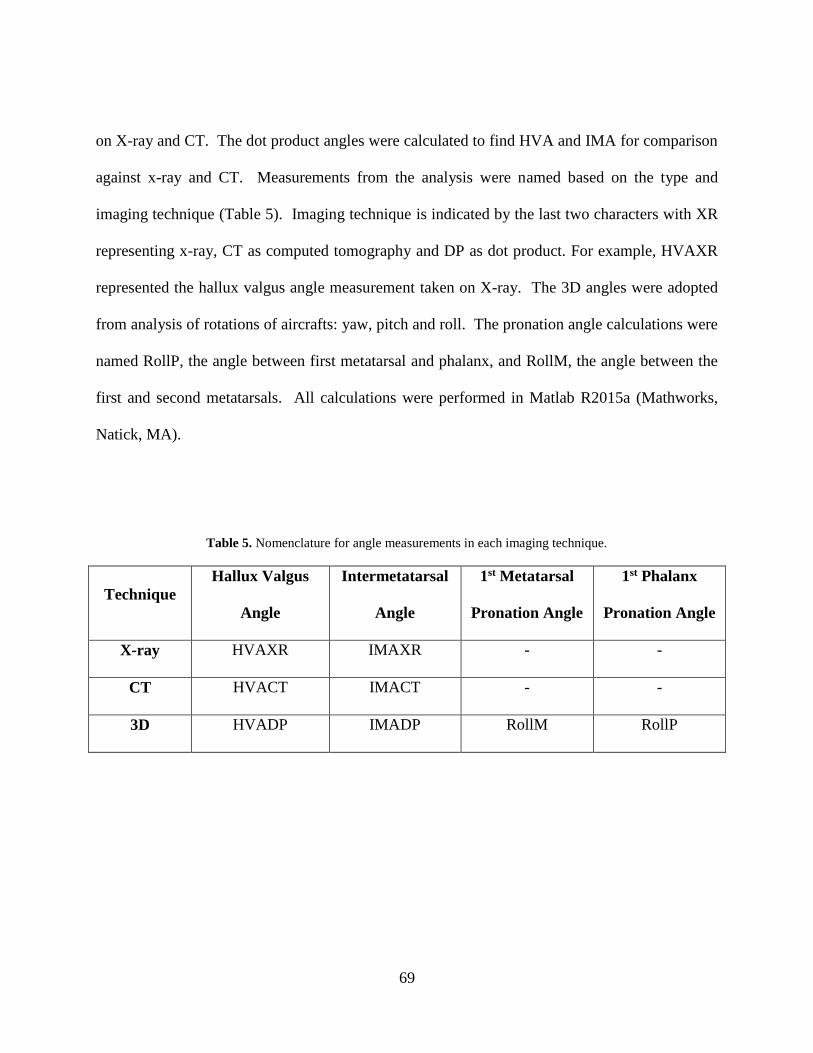
69
on X-ray and CT. The dot product angles were calculated to find HVA and IMA for comparison
against x-ray and CT. Measurements from the analysis were named based on the type and
imaging technique (Table 5). Imaging technique is indicated by the last two characters with XR
representing x-ray, CT as computed tomography and DP as dot product. For example, HVAXR
represented the hallux valgus angle measurement taken on X-ray. The 3D angles were adopted
from analysis of rotations of aircrafts: yaw, pitch and roll. The pronation angle calculations were
named RollP, the angle between first metatarsal and phalanx, and RollM, the angle between the
first and second metatarsals. All calculations were performed in Matlab R2015a (Mathworks,
Natick, MA).
Table 5. Nomenclature for angle measurements in each imaging technique.
Technique
Hallux Valgus
Angle
Intermetatarsal
Angle
1st Metatarsal
Pronation Angle
1st Phalanx
Pronation Angle
X-ray HVAXR IMAXR - -
CT HVACT IMACT - -
3D HVADP IMADP RollM RollP

70
5.4 STATISTICAL ANALYSIS
The results from both clinical studies were further examined in statistical analyses. In both
cases, the hallux valgus patient group (n = 10) was compared against the normal group (n = 10).
All analyses were conducted with SPSS (Version 22.0. Armonk, NY: IBM Corp.).
5.4.1 Clinical Measurement Analysis
All statistical analyses were conducted in SPSS for Windows, Version 24.0 (IBM Corp.,
Armonk, NY). The data was analyzed to determine differences regarding three independent
variables: foot group (hallux valgus or normal), imaging technique (angular measures from x-
ray, CT or 3D model) and weightbearing condition (weightbearing or non-weightbearing). The
imaging technique variable identified the means used to calculate HVA and IMA.
If the reported kappa value was excellent or good (>0.80) the coordinate data was
averaged between the raters. The non-weightbearing and weightbearing angles (Yaw and Roll)
calculated by 3D for both foot groups (hallux valgus vs normal) were tested with Friedman
ANOVAs. The data was further explored with Wilcoxon signed ranked post-hoc tests to
elucidate any differences between group P-values. The weightbearing measurements from X-ray,
CT and DP were tested with Pearson’s correlation, Friedman ANOVA and post hoc analysis
with Wilcoxon signed ranked tests to compare the imaging technique and foot group. P-values
were reported. All Friedman ANOVA were significant if the p-value was less than 0.05. The
post-hoc analyses were significant if the p-value was less than the adjusted threshold after

71
Bonferroni correction. The relationship between the yaw and roll measurements were tested to
determine their level of correlation. Pearson’s correlations were conducted on the YawM with
RollM and YawP with RollP in normal and hallux valgus groups. The r-values were reported.
5.4.2 Densitometric Analysis
The statistical analysis was conducted within and between groups. The within group analysis
compared the average values of the measurements taken at the cuneiform and at the metatarsal
head and base. Within the sagittal plane, the dorsal and plantar average values were compared
for both groups. Within the transverse plane, the medial and lateral average values were
compared for both groups. The between group analysis compared the average normal values
against the average HV value at the same location. Independent one way, t-tests were conducted
for the within (dorsal versus plantar and medial versus lateral) with location as the independent
variable. Independent t-tests were conducted for the between group analysis (normal versus HV)
with patient group as the independent variable.

72
6.0 METHODLOGY FOR FEA MODELING
The second aim was to conduct a static structural analysis with a goal of developing predictions
of the progression of HV deformities. We sought to find the contact stress between joints of the
first ray. The model was validated on the basis of its ability to approximate the foot’s mechanical
behavior. The models were loaded with bodyweight and the deformed foot’s bone positions were
compared with full weightbearing CAD models of the same foot for validation.
6.1 MODEL CREATION
A three dimensional model was created from each patient’s DICOM images. The models for
both groups of normal and HV patients were used to determine the bone orientation by landmark
analysis. Two models, an HV solid model and normal solid model, were extended to an FEA
model and concomitant analysis. The FEA simulations were conducted to elucidate stresses at
the joints of the first ray.

73
Figure 22. Workflow process to create FEA models from the CT scans.
6.1.1 CT to CAD Process
CT scans had to be processed after each set of images was collected. Each patient’s images were
a series of DICOM files. The DICOM file contained planar cross sectional images of the
scanned foot and ankle, headers of the patient’s demographics and imaging protocol information
supplied to the x-ray technician. The creation of a volume was initiated by importing the files
into image processing software, Mimics (Materialise NV, Leuven, Belgium). The first step was
the identification of the direction of each plane, e.g. the transverse cross section designated as
medial/lateral or anterior/posterior. The CT coordinate system was confirmed as the global
coordinate system and the importation process was completed. In Mimics, reconstruction of the
DICOMs appeared as pixels representing scanned components in all slices in three planes: axial,

74
coronal and sagittal. Bodies (bone or soft tissue) were viewable and indicated in each slice, in
each of the three planes. The segmentation process involved identifying the geometry of a bone
in a given slice, outlining groups of pixels in the plane and eliminating extraneous pixels. The
segmentation then identified the first and second rays in each slice, from the distal phalange
through the cuneiform. Next, a mask, a collection of pixels, from all connected pixels was
created for each bone. The metatarsals and phalanges retained the medullary canals. A three
dimensional bone was created by taking a mask, combining the group of slices into a set of
voxels and creating a volume. The process was repeated and completed until all bones were
represented as three-dimensional volumes.
The segmentation process produced a very primitive shape for the individual bones and
required further processing. The files for the bone models were saved as. stl files. In general, in
an .stl file format, a volume is represented by a surface of triangles. Here, the output file
produced a distorted volume of bone. An extension of Mimics called 3Matic (Materialise NV,
Leuven, Belgium) was used to clean (remove self-intersecting faces, remove overlapping
triangles, remove non manifold edges and vertices) and manually smooth the shape of the bones.
They were then imported to Geomagic Quality (3D Systems, Rockhill, SC) image processing
software and were converted to IGES file type, the preferred finite element format.
Typically, CT imaging is preferred for high resolution, easily viewable images of human
bone. However, it is not ideal for visualizing soft tissue, which can be indistinct on a CT image.
In our case, the cartilage layer was manually created in SolidWorks (Dassault Systèmes,
Waltham, Massachusetts) or Ansys DesignModeler. Given that IGES files are formatted as a
collection of triangles used to produce a volume, the surface of the triangular patch that
comprised the outer bone volume at the joint surface was used to create the shape of the

75
respective cartilage. The patch size was selected to cover the anatomical area of each respective
bone’s cartilage [94] and duplicate the anatomy of the joint articular surfaces. After importing
the bone file into SolidWorks, the triangular patch elements were selected at the proximal and
distal end of the bone to reflect the anatomic shape. Sets of triangular patches were grouped
together as a layer offset from the original surface by 0.0 mm. This choice of offset length
allowed the surface layer closest to the bone to remain in contact but produced a separate volume
that later became the corresponding cartilage. The layer was then extruded to its anatomical
thickness [73]. The anatomical thickness was determined by calculating the space between
bones at the joints. The cartilage thickness used in the model was 50% of the calculated value.
Each layer of cartilage was saved as a separate IGES file. This process was repeated for all
bones with cartilage in the tarsometatarsal, metatarsophalangeal and metatarsosesamoidal joints.
All files, both bone and cartilage, were imported to Ansys Mechanical APDL 16.0 (Ansys, Inc.,
Canonsburg, PA) within the default tolerance and saved again as assembly of the first two rays
of the foot. They were exported and saved as an IGES file.
The file of the first two rays was imported to Ansys Workbench 16.1 (Ansys, Inc.,
Canonsburg, PA), a schematic for structuring multiphysics analysis. Within Workbench, a static
structural analysis was used to conduct the FEA simulations. The model was opened in Ansys
APDL 16.1, the physical simulation package available within Workbench. The ligaments and
contacts between the joints were added and the method of computation was selected. The
location of the ligaments, modeled as tension only links, corresponded to that of the foot
anatomy [17]. The contact surface pairs were established between (1) respective layers of
cartilage, in contact at a joint and (2) cartilage in contact with a separate bone surface and (3)
bone and cartilage of the same bone. The (1) and (2) contacts behaved as frictionless contact

76
surfaces while (3) was a “bonded” contact such that the most exterior points of an individual
surface on a body in contact with the surface of the other body, did not separate.
6.1.2 CAD to FE Process
Material Properties
The material properties were taken from previously reported models in the literature and
data from biomechanical tests. Bone and cartilage were modeled as homogenous, isotropic and
linear elastic materials. The ligaments were modeled using (1) linear springs, which were later
amended to be (2) tension only springs. The applied values of stiffness, Young’s modulus and
Poisson’s ratio used for bone, cartilage and ligaments are shown in Table 6.
Table 6. Material properties for the finite element models.
Young’s Modulus Poisson’s Ratio Stiffness
Ground 68900 MPa 0.35 -
Homogenous Bone 7300 MPa 0.4 -
Cartilage 0.8 MPa 0.4 -
Sesamoid Cartilage 1.01 MPa 0.07 -
Ligament (reported) 260 MPa
Ligament* - - T: 1500 N/mm
C: -5 N/mm
*Stiffnesses were applied to ligaments without reported areas and lengths.

77
The ligaments were formally modeled as quasi-tension only spars, more commonly
known as two-dimensional links. Stiffness and damping coefficients (c = 0) governed the
behavior of the ligaments. Two types of tensile stiffness values were input as tabular data. The
tensile stiffnesses for ligaments with previously reported morphological data in biomechanical
studies (Table #) were derived from a modulus of 260 MPa. Ligaments without reported
morphological data were assumed to have a tensile stiffness of 1500 N/mm. Both reported and
unreported ligaments were modeled with compressive stiffness of 5 N/mm. Because, the
ligaments were represented by multiple springs, the stiffness values input as K/n, with K as the
ligament stiffness and n as the number of springs used to model the ligament. The length of the
link was the reported anatomic length of the individual ligaments at each modeled joint. The
unreported ligament stiffness values were determined by using a uniform modulus (260 MPa)
and measured area and length data (Table 7). All ligaments at the metatarsosesamoidal and
tarsometatarsal joints were represented (Table 8).
Table 7. Material properties for the finite element models.
Ligament Area-Length Ratio Estimated Stiffness
Dorsal (Kura) 11.32 mm 2,943.2 N/mm
Lisfranc (Kura) 18.54 mm 4,820.4 N/mm
PC1M1 (Mkandawire) 4.76 mm 1,237.6 N/mm
DC1M1 (Mkandawire) 3.21 mm 834.6 N/mm
MC1M1 (Mkandawire) 2.82 mm 733.2 N/mm
78
Both ends of the link were attached to bone surfaces with pinball regions, or a group of
nodes, on the bone surface. The pinball region, a uniform sphere defined by a user input radius,
and used merely as a visual aid, originated from a selected vertex on the solid model. All nodes
within the pinball region stemming from the vertex were selected as spring endpoints and
attached remotely (known as a remote point when used with a single point). The remote
attachment was defined as an optional boundary condition wherein the endpoint of a spring was
an abstractly scoped connection to a solid model. Therefore, the remote attachment between the
vertex and spring endpoint was distributed among the surface nodes within the pinball region on
the exterior surface. The attachment was a surfaced based constraint, similar to a multipoint
constraint where the forces and displacements are applied remotely, distributed to contact nodes
through shape functions and had full translational and rotational degrees of freedom. The size of
the pinball region was defined such that it represented the area of the ligament origin/insertion.

79
Table 8. Ligaments of interest in the first and second rays of the forefoot.
Origin Insertion
1 Lateral Medial Cuneiform Dorsal Inter Cuneiform
2 Medial Cuneiform Anterolateral Second Metatarsal
3 Dorsal First Metatarsal Dorsomedial Medial Cuneiform
4 Dorsal Second Metatarsal Anterolateral dorsum of the Medial Cuneiform
5 Dorsal Second Metatarsal Anterolateral dorsum of the Inter Cuneiform
6 Plantar base of the lateral half of First
Metatarsal
Plantar (near articular surface) Medial
Cuneiform
7 Inferolateral Cuneiform Inter Cuneiform (Lisfranc)
8 Lateral surface of the Medial Cuneiform Plantar Second Metatarsal
9 Lateral proximal phalanx Lateral proximal metatarsal
10 Medial proximal phalanx Medial proximal metatarsal
11 Proximal Medial Sesamoid Distal First Metatarsal
12 Distal Medial Sesamoid Proximal First Phalanx
13 Proximal Lateral Sesamoid Distal First Metatarsal
14 Distal Lateral Sesamoid Proximal First Phalanx
15 Lateral Medial Sesamoid Medial Lateral Sesamoid

80
Meshing
The bones and cartilage were modeled with ANSYS SOLID186 elements, a homogenous, 10-
node structural solid tetrahedral element. Each node in the element had three translational
degrees of freedom and allowed for the input of Young’s Modulus and Poisson’s ratio. The
ligaments were modeled with a variation of the COMBIN14 (linear spring) called a LINK180
(tension only spar). COMBIN14 was a spring-damper, uniaxial tension-compression element
with up to 3 degrees of freedom at both nodes. This massless element was used with the damping
coefficients zeroed. LINK180 was an altered version of the COMBIN14 element to eliminate the
compression of the spring element. LINK180 was a 3D element, had three degrees of freedom at
each node and did not allow bending. The shape function and detailed descriptions can be found
in the ANSYS Theory Reference guide and Element Reference Guide respectively.
The solid element mesh was generated for bone and cartilage by an automatic meshing
tool in Ansys. The volumes of different bones were not in direct contact with each other and the
expected outputs were stresses in regions as a result of tension, compression and bending.
Cartilage surfaces of different bones were in contact with each other due to loading and the
expected outputs were stress due to pressure from the interaction with other cartilage surfaces.
As a quality control measure, the element shapes were monitored and inspected to ensure the
aspect ratio of the individual tetrahedral elements was within 0.8-1.2. The element length chosen
for the mesh was based on a mesh convergence study (Figure 23). Single, isolated peaks were
found in the mesh convergence at 0.125 mm and 0.075 mm in the normal model (Figure 24), but
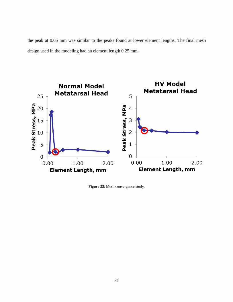
81
the peak at 0.05 mm was similar to the peaks found at lower element lengths. The final mesh
design used in the modeling had an element length 0.25 mm.
Figure 23. Mesh convergence study.

82
Figure 24. Mesh convergence peaks.
Contacts were created between (1) interacting cartilage surfaces and (2) bone and the
respective cartilage surfaces. The former interaction was modeled with frictionless contact
between the two faces. The contact between bone and respective cartilage was defined as a
bonded contact. This type of contact ensured the adjacent boundaries of surface 1 and surface 2
moved together and was programmed to prevent sliding or separation between the edges and
surfaces.

83
Table 9. Description of the FEA models used in the study.
HV Patient Normal Patient
Model Identification HVPatient_NonWB NormalPatient_NonWB
Bones MTS Model
5
TMT Model
4
MTS Model
5
TMT Model
4
Cartilage 2 2 2 2
Ligaments 7 6 7 6
Type Deformable Deformable
Zero State (3D) HV: -25.63°
IM: 14.05°
HV Pro: -7.67°
IM Pro: -25.57°
HV: -10.27°
IM: 11.44°
HV Pro: -2.81°
IM Pro: -28.99°
Loaded State (3D) HV: -25.85°
IM: 14.70°
HV Pro: -11.01°
IM Pro: -19.48°
HV: -10.74°
IM: 11.27°
HV Pro: -0.44°
IM Pro: -26.20°
Loading Condition 80 N; Ramped Nodal Load 80 N; Ramped Nodal Load
Mesh Density Nodes: 79377
Elements: 41932
Nodes: 67908
Elements: 36584
Element Name SOLID187 SOLID187
Element Type/Shape 10 Node Tetrahedral; 0.25 mm 10 Node Tetrahedral; 0.25 mm
Convergence Criteria Software Default Software Default

84
6.2 MODELING CONDITIONS AND SIMULATIONS
The purpose of the boundary and loading conditions implemented in the model were to produce
the pressures associated with interaction at the metatarsosesamoid and tarsometatarsal joints
during weightbearing. Therefore, the conditions correspond to loads that approach the magnitude
found during standing. Both models were similarly configured and with slight differences
integrated to better reflect the physiology of hallux valgus.
6.2.1 Boundary Conditions
The displacement and rotational boundary conditions were implemented to simulate the anatomy
and physiology of the foot during stance. In both the HV and normal models of the
metatarsosesamoid joint (Figure 25 and 26), the second rays (which includes the second
phalanges, metatarsal and cuneiform) were rigid bodies fixed in space. The proximal first
metatarsal and the distal first phalanx were also fixed as shown in yellow. The proximal region
of the proximal phalanx and distal region of the first metatarsal were deformable with nodes free
to move. All cartilage surfaces within the metatarsophalangeal and metatarsosesamoid joints
were free to deform.
Both HV and normal tarsometatarsal joint models (Figure 27 and 28) were also
comprised of deformable bodies with boundary conditions established such that the second ray
was unable to displace. The medial cuneiform was fixed at the proximal region and the
metatarsal and phalanges were free to displace.

85
Figure 25. Boundary conditions of the HV model.
Figure 26. Boundary conditions of the normal model.

86
Figure 27. HV (left) and Normal (right) MTS Model.
Figure 28. HV (left) and Normal (right) TMT Model.

87
Figure 29. Loading conditions of the HV model.
Figure 30. Loading conditions of the normal model.

88
The loading conditions were implemented to simulate the anatomy and physiology of the
foot while under load during stance. The metatarsosesamoid models were loaded with a ramped
force applied through a set of nodes on the plantar surface of the sesamoids (Figure 29 and 30).
The nodal force was applied as a linearly increasing load with the force rising at each of 20 time
steps. The normal model was loaded with 60% of the nodal force applied to the medial sesamoid
and 40% beneath the lateral sesamoid. In the HV model, 95% of the nodal force was applied to
the medial sesamoid and 15% to the lateral sesamoid. The magnitude of loads for the MTS
models was 75 N on each sesamoid pair. The magnitude of loads for the TMT models was up
to75 N.
The displacement of the models was validated by comparing the kinematic position of the
FEA output against weightbearing CAD models of the same patient. The post-processed FEA
models were exported from Ansys Mechanical APDL to Ansys Modeler. Afterwards, the models
were exported to Geomagics for comparison with the weightbearing CT scan. The positions of
the sesamoids in the MTS models and position of the metatarsal and phalanx were compared.
The intermetatarsal angle in the TMT models was compared to the weightbearing CAD models.
6.2.2 Data Analysis
The post processing data analysis of the models included comparing the mechanical response of
all models to previous FEA models and clinical studies of plantar pressure during standing. All

89
post processing data analyses were performed in Matlab 2016a (Mathworks, Natick, MA). We
reported peak stresses and contact pressures.

90
7.0 CLINICAL RESULTS
7.1 THREE-DIMENSIONAL MEASUREMENTS
The interrater reliability between the raters of the weightbearing and non-weightbearing angles
calculated from the landmark coordinate data was excellent (kappa > 0.9). Therefore, the
coordinate data was averaged between the two raters for analysis.
RollP for hallux valgus and normal groups were 34.2 ± 10.7 and 11.5 ± 3.5 respectively
(p = 0.023) (Figure 31). Weightbearing group averages for RollM were 19.1 ± 7.1 and 27.3 ±
10.6 for the normal and hallux valgus groups respectively (p = 0.043) (Figure 321). The
regression of RollM on IMAXR was found to be very weak (both normal and HV: r < = 0.000
N/-0.072 HV) indicating that 3D first metatarsal pronation had no relationship with
intermetatarsal angle measured on x-ray (Figure 33). The regression of RollP on HVAXR was
also found to be weak (r = 0.256 N/-0.156 HV) indicating that 3D first metatarsal pronation had
a poor relationship correlation with HV angle measured on x-ray (Figure 332).

91
The 3D angles were calculated for weightbearing and non-weightbearing models for each
subject. ANOVAs revealed a significant difference weightbearing in RollM for the hallux
valgus group (p = 0.034). All others were not significant in comparisons of weightbearing to
non-weightbearing.
Figure 31. Pronation of the first phalanx relative to the first metatarsal.

92
Figure 32. Pronation of the first phalanx relative to the first metatarsal

93
Figure 33. Correlation of the intermetatarsal angle measurement from x-ray versus first metatarsal
pronation angle.
Figure 34. Comparison of group average angular measurements for each imaging technique.

94
The ANOVA of between IMA and HVA found differences due to patient group (Normal
or HV subjects, p = 0.001) and clinical angle measure (p = 0.001 - CAD, X-ray, CT) (Figure 34).
The only significant differences in clinical angle IMA and HVA measures were found in IMA
between IMADP against IMACT (p = 0.022). The measurements were well correlated between
techniques methodologies (Figure 35) with the strongest relationship found in the x-ray and dot
product method in the HVA and IMA angles (r > 0.80).

95
A.
B.
C.
D.
Figure 35. Correlation of the imaging techniques.

96
7.2 DENSITOMETRIC ANALYSIS
The dataset was normally distributed (p > 0.05) and met the assumption of homogeneity of
variances (p > 0.05). The HV and normal groups were found to be more dense dorsally than
plantarly at the metatarsal base and cuneiform (p < 0.04). In the mediolateral direction, the
medial base was more dense than lateral base in both groups. At the cuneiform, the normal group
was more dense laterally whereas the HV group was more dense medially.
The mean densities of both HV and normal groups are shown above for the medial and
lateral comparison (Figure 36) and dorsal and plantar comparison (Figure 37). The first four
boxes in each plot are averages found at the metatarsal base and the last four boxes are averages
found at the cuneiform. The plots of average densities are shown with standard deviation error
bars. The dots indicate maximum (95th percentile) and minimal (5th percentile) densities values
found at each region.

97
Figure 36. Mean densities of both HV and normal.

98
Figure 37. Mean densities of both HV and normal groups.
ANCOVAs found significant differences (p < 0.045) in the comparison of mediolateral
and dorsoplantar density pairs respectively for both the metatarsal and cuneiform within the
normal and HV groups. At the metatarsal base, group had a significant effect on the density
differences of both pairs (p < 0.02). At the cuneiform, group had a significant effect on the
density differences of the dorsoplantar densities. Age had a significant effect on differences in
the dorsoplantar comparison of the metatarsal base, but, elsewhere, age did not have a significant
effect (p > 0.08).

99
Figure 38. Dorsal and plantar density changes at the metatarsal head, base and cuneiform
Figure 39. Medial and lateral density changes at the metatarsal head, base and cuneiform

100
Differences in density at the metatarsal head, base and cuneiform are further illustrated in
Figure 38. The top figure shows the difference in average Hus and the shift in density between
HV and normal groups. Positive values reflect higher density dorsally and negative values reflect
higher density plantarly. The bottom figure (Figure 39) shows the difference in average HUs and
the shift in density between HV and normal groups. Positive values reflect higher density
medially and negative values reflect higher density laterally.
Regressions of density against normalized anatomic position illustrated the significant
results at the metatarsal head (Figure 40), metatarsal base and cuneiform (Figure 41) in the
sagittal and transverse planes. The regression lines are lines representing the mean values trends
of density in a specific (normal or HV) group at a specific location (dorsal or plantar). The plots
at the top of the figure show the trend of density across a normalized width in the mediolateral
direction. The normalized width extends in the direction such that 0 corresponds with the most
medial slice. The normalized width at 1 corresponds with the most lateral slice. The plots at the
bottom of the figure show the trend of density across a normalized length in the superoinferior
direction. The normalized height extends in the direction such that 0 corresponds with the most
dorsal slice. The normalized height at 1 corresponds with the most plantar slice. For example,
the normal and HV groups both demonstrated significant differences in dorsal and plantar
densities within each group as revealed by the difference in intercepts between the red/purple
versus blue/green lines in Figure #b. Similarly, the red line of dorsal density of the HV group had
a larger intercept than the purple line of the dorsal density of the normal group.

101
Figure 40. Scatter plot and regression of the density in both HV and normal groups.

102
Figure 41. Scatter plot and regression of the density in both HV and normal groups.

103
8.0 FINITE ELEMENT ANALYSIS RESULTS
The normal and HV models of the foot showed the differences in mechanical response of the
metatarsosesamoidal and tarsometatarsal joints simulating load while standing. Both models
were validated by comparison against by measured values from CAD models of the foot during
weightbearing. A sensitivity analysis was reported for the metatarsosesamoidal models to show
how the cartilage modulus of elasticity E affects the mechanical response of the joint due to
standing. The peak von Mises stress and contact pressures were reported for both
metatarsosesamoidal and tarsometatarsal models.
8.1 METATARSOSESAMOIDAL MODEL
8.1.1 Metatarsal Head and Sesamoids Contact
The average contact pressure for both HV and normal models were calculated (Figure 42). At
the lower sesamoid loads, the average contact pressure of the medial sesamoid in the normal
model was largest relative to both models. At the higher sesamoid loads, the pressure was larger
at the medial sesamoid of the HV model and found to be nearly 2 MPa at 80 N sesamoid load.
The average contact pressure in the lateral sesamoid of the normal model was between 0.2 and

104
0.7 MPa across increasing sesamoid loads. The average contact pressure was lateral sesamoid of
the HV model was below 12 kPa.
Figure 42. Average contact pressure comparison of the normal (left) and HV (right) models.
The average contact area for the medial sesamoids of both the HV and normal models
were similar as the load increased (Figure 43). In the normal model, the area was found to be 18
mm2 at the lowest measured sesamoid load and nearly 35 mm2 at the highest sesamoid load. The
range of average contact area in the lateral sesamoid of the normal model was between 9 and 17
mm2. In the HV model, the contact area was found to be nearly 20 mm2 at the lowest measured
sesamoid load and nearly 32 mm2 at the highest sesamoid load. The average contact area of the
lateral sesamoid in the HV model did not exceed 1 mm2.

105
Figure 43. Average contact area comparison of the normal (left) and HV (right) models.
The average contact force in both HV and normal models was calculated and reported
(Figure 44). In the medial sesamoids of both models, the average contact force increased as the
force on the sesamoids increased. In the normal model the average contact force, 40 N, was
largest at 80 N. At the same load in the HV model, the contact force was found to be nearly 60
N. The rate of increase of contact force was greater in the HV model. At the lateral sesamoid, in
the normal model the contact force was below 11 N and in the HV model was well below 1 N.

106
Figure 44. Average contact force comparison of the normal (left) and HV (right) models.
A sensitivity analysis was conducted to compare the contact pressure, area and force of
the metatarsosesamoid interaction in three cases: (1) standard cartilage modulus E, (2) modulus
reduced by 10% and (3) modulus increased by 10%. The average contact pressures for all
simulations of 90% E, 100% E and 110% E, are shown in Figure 45. The contact pressure at the
metatarsal was calculated for metatarsal head at the interface between the cartilage of both
sesamoids. The contact pressures in the medial sesamoids were largest in the models with varied
modulus, 90% E and 110% E. In the lateral sesamoid of the normal model, the average contact
pressures were similar in the model with standard E and with E increased by 10%. Overall, the
peak and average contact pressures were greatest at the medial sesamoid in the HV model. Only
at 60 N loading, were the average contact pressures in the medial sesamoid in both HV and

107
normal models were similar. In assessing the HV model individually, the average contact
pressure of the lateral sesamoid was less than 12 kPa under maximum loading of 80 N.
Figure 45. The average contact pressure comparison of the normal (left) and HV (right) models with modified
moduli of elasticity.
The average contact area for each simulation where the cartilage modulus was varied,
90% E, 100% E and 110% E, is shown in Figure 46. Average contact area increased proportional
to increasing load in all cases with exception of the HV medial sesamoid. The average contact
area was largest in the models with E and E increased by 10%. In the 90% E simulations, medial
sesamoid contact area differed mostly at 60 N. Elsewhere the area was similar for both HV and
normal medial sesamoids. In the 100% E and 110% E simulations, the medial sesamoid areas

108
were similar between HV and normals at various loads. The largest change in area across loading
conditions occurred in the medial sesamoid of the normal in the 100% E case. At 20 N, the
average contact area was 17 mm2 and doubled under 80 N. Overall, the largest contact areas
respectively were found in the medial sesamoid of the both HV and normal models. At 80 N, the
average contact area at the medial sesamoid in both HV and normal models was between 31 and
34 mm2. The smallest contact areas were found in the lateral sesamoid of the HV model, which
were well below 1 mm2.
Figure 46. The average contact area comparison of the normal (left) and HV (right) models with modified moduli of
elasticity.

109
The average contact forces for each simulation where the cartilage modulus was varied,
90% E, 100% E and 110% E, are shown in Figure 47. The average contact force at the medial
sesamoid was largest, 32 N, at 80 N sesamoid force in the models with E increased by 10%. At
lower sesamoid forces, the average contact force at each sesamoid was similar for each
simulation of varied E except for the case of the medial sesamoid in the normal model at 40 N.
In the lateral sesamoid of the normal model, the contact force was similar between each
sesamoid force within each simulation of varied E. In the normal model, at 80 N in the medial
sesamoid, the contact force doubled when using 110% E. In the HV model, the medial sesamoid
increased linearly with increasing E. The contact force of the lateral sesamoid in the HV model
measured well below 1 N.
Figure 47. The average contact force comparison of the normal (left) and HV (right) models with modified moduli
of elasticity.

110
The nodal force input to both the HV and normal models was applied through the plantar
surface of the sesamoid. The sesamoids were connected to the metatarsal by springs elements
with quasi-tension only stiffness. In each simulation, the applied force on the sesamoid was not
equal to the contact force on the metatarsal head. The remaining force, the difference between
the applied force and contact force, was absorbed by the spring ligaments in the model.
8.1.2 Metatarsal Head and Sesamoids Cartilage von Mises Stress
The peak von Mises stresses across both HV and normal models were between 0.5 MPa and 3
MPa as the sesamoid loading increased (Figure 48). The medial sesamoid of the HV model had
the largest increase in pressure. At lower sesamoid loads, the peak von Mises stress was higher
in the metatarsal of the normal model. At 20 N, the von Mises stress on at the metatarsal head
was 0.5 MPa and 0.9 MPa respectively for the HV and normal models. The peak stress for each
of the corresponding sesamoid loads occurred in the region of the metatarsal where the medial
sesamoid made contact. At the 80 N loading, peak von Mises stress in the metatarsal head of the
HV model, 2.7 MPa, was larger than in that of the normal model, 2.25 MPa. At the cartilage of
the medial sesamoids, in both HV and normal models, the peak von Mises stresses were similar
at 20 N and 40 N. Beyond that point, the peak values were larger in the HV model. The peak von
Mises stress in the lateral sesamoid of the HV model did not exceed 1 kPa.
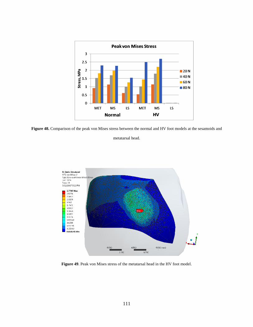
111
Figure 48. Comparison of the peak von Mises stress between the normal and HV foot models at the sesamoids and
metatarsal head.
Figure 49. Peak von Mises stress of the metatarsal head in the HV foot model.

112
Figure 50. Peak von Mises stress of the sesamoids in the HV foot model.
Figure 51. Peak von Mises stress on the metatarsal head in the normal foot model.

113
Figure 52. Peak von Mises stress on the sesamoids in the normal foot model.
Figure 53. Maximum shear stress in the HV model.

114
Figure 54. Maximum shear stress in the normal model.
Figure 55. Peak von-Mises stress distribution at the Metatarsal Head in the HV Model.

115
Figure 56. Peak von Mises stress distribution at the metatarsal head in the normal model.
8.1.3 FEA Model Validation
The metatarsosesamoidal model was validated by comparing the position of the sesamoids in the
FEA and CAD models. The distance between the calculated center points of the sesamoids and
metatarsal head are shown in Table 10. The largest difference in position was found between the
lateral sesamoid in the HV model, where the experimental error between the positions of the
sesamoids in both models was below 5%.

116
Table 10. Validation of the metatarsosesamoidal finite element models.
Distance from the metatarsal head
X (mm) Y (mm) Z (mm) Error
HV
Model
Medial
Sesamoid
FEA 2.29 5.73 -11.38 <%
CAD 2.48 4.87 -11.81
Lateral
Sesamoid
FEA 12.92 6.22 -5.99 <%
CAD 12.49 5.80 -6.38
Normal
Model
Medial
Sesamoid
FEA -2.20 7.50 -12.02 <%
CAD -2.78 7.75 -12.01
Lateral
Sesamoid
FEA 9.69 6.90 -9.33 <%
CAD 9.39 7.84 -9.01
8.2 TARSOMETATARSAL MODEL
8.2.1 Metatarsal Base and Cuneiform Contact
The average pressures were calculated at the contacts in the tarsometatarsal joint. In the normal
model, the contact pressure on the metatarsal base was larger than on the cuneiform at each input
load (Figure 57). The maximum contact pressures on the cuneiform and metatarsal base were
0.412 MPa and 0.523 MPa respectively. In the HV model, the contact pressure was larger on the
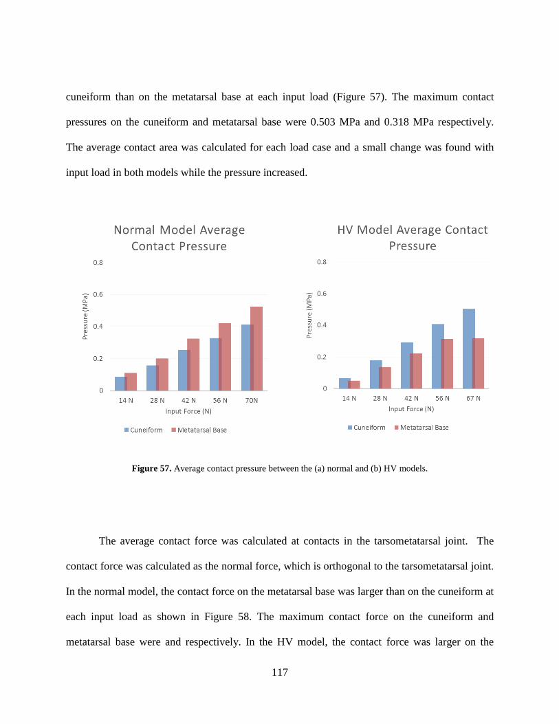
117
cuneiform than on the metatarsal base at each input load (Figure 57). The maximum contact
pressures on the cuneiform and metatarsal base were 0.503 MPa and 0.318 MPa respectively.
The average contact area was calculated for each load case and a small change was found with
input load in both models while the pressure increased.
Figure 57. Average contact pressure between the (a) normal and (b) HV models.
The average contact force was calculated at contacts in the tarsometatarsal joint. The
contact force was calculated as the normal force, which is orthogonal to the tarsometatarsal joint.
In the normal model, the contact force on the metatarsal base was larger than on the cuneiform at
each input load as shown in Figure 58. The maximum contact force on the cuneiform and
metatarsal base were and respectively. In the HV model, the contact force was larger on the

118
cuneiform than on the metatarsal base at each input load as shown in Figure 58. The maximum
contact forces on the cuneiform and metatarsal base were 148 MPa and 145 MPa respectively.
The average contact area was calculated for each load case and a small change was found with
input load in both models.
Figure 58. Average contact force between the (a) Normal and (b) HV models.
8.2.2 Metatarsal Base and Cuneiform von Mises Stress
The von Mises stress was calculated at the metatarsal base and cuneiform in both foot models.
In the normal model, higher stress was found in the dorsal to lateral region of the surface of the
cuneiform (Figure 59). The lower stresses appeared in the plantar region of the cuneiform. In the
metatarsal base, higher stress was found in the dorsal region of the surface (Figure #). Stresses

119
were lowest in the medial and lateral regions of the metatarsal base. In the cuneiform of the HV
model, the peak von Mises stresses appeared plantarly, towards the medial side of the plantar
region on the metatarsal base (Figure 60). On the surface of the cuneiform, the peak stresses
were concentrated in the plantar and medial regions (Figure 61).
Figure 59. Von Mises stress in the cuneiform of the normal foot model.

120
Figure 60. Von Mises stress in the metatarsal base of the normal foot model.
Figure 61. Von Mises stress in the cuneiform of the HV foot model.

121
Figure 62. Von Mises stress in the metatarsal base of the HV foot model.
The trend of von Mises stress across the cuneiform was measured in both models with
“path lines” across the subchondral surface in the mediolateral and dorsoplantar directions. The
averages of the path lines were calculated by dividing the nodal stress on the path line into two
sets and taking the average of each set (Figure 63). Each side represented an average on the
medial or lateral and dorsal or plantar region of the bone. In the normal model, the stress was
higher in the lateral area of the cuneiform compared to the medial area. The stress was higher in
the dorsal area of the metatarsal base compared to the plantar area (Table 11). In the HV model,
the stress was comparable on both sections of the cuneiform in all directions (Table 12). The
average stress on the medial and lateral sections of the path lines were similar as well as the
dorsal and plantar sections of the path lines.

122
Table 11. Path line averages of von Mises Stress calculated in cuneiform of normal model.
Lateral Area Medial Area Dorsal Area Plantar Area
Superior Line 0.91 MPa 0.74 MPa Lateral Line 0.97 MPa 0.58 MPa
Central Line 1.08 MPa 0.87 MPa Central Line 0.94 MPa 0.64 MPa
Inferior Line 1.26 MPa 1.04 MPa Medial Line 1.04 MPa 0.85 MPa
Table 12. Path line average of von Mises Stress calculated in the cuneiform of the HV model.
Lateral Area Medial Area Dorsal Area Plantar Area
Superior Line 0.364 MPa 0.312 MPa Lateral Line 0.451 MPa 0.477 MPa
Central Line 0.459 MPa 0.676 MPa Central Line 0.487 MPa 0.750 MPa
Inferior Line 0.450 MPa 0.476 MPa Medial Line 0.495 MPa 0.455 MPa

123
Figure 63. Path lines in the cuneiform.
8.2.3 FEA Model Validation
The tarsometatarsal models were validated by comparing the intermetatarsal angle of the FEA
models to that of the measurements from weightbearing CAD reconstructions. The calculated
intermetatarsal angles are shown in Table 13. The experimental error between the angles was
below 2% for both the normal and HV models.

124
Table 13. Validation of the tarsometatarsal models.
Trial 2 Error
Normal Model Unloaded 11.44° -
CAD 11.27° -
FEA 11.14° 2%
HV Model Unloaded 14.05° -
CAD 14.70° -
FEA 14.61° 1%

125
9.0 DISCUSSION
The results found from our study are compared and contextualized here in the discussion. We
found a method to measure pronation of the long bones in the first ray and reported the
differences between normal and HV groups. We measured the density at the metatarsal head and
tarsometatarsal joints and reported differences in the densitometric profiles in our normal and
HV groups. Lastly, we modeled the forefoot in a finite element model and measured differences
in contact mechanics between a normal and HV models.
9.1 INFERENCES FROM THE ANGLE MEASUREMENTS RESULTS
Our study is the first to calculate pronation of the first metatarsal in vivo using a 3D
methodology, within a hallux valgus population. This three-dimensional analysis of the HV
triplanar deformity offers a result that is independent of the choice of viewing plane, producing a
set of angular measurements to comprehensively describe the deformity. We found the
orientation of the bones in the first ray by calculating the position of individual bones within a
single foot and comparing their relative positions. We measured pronation of the first phalanx
and first metatarsal in a normal group for comparison against the hallux valgus patient group to

126
better understand how the deformity evolves. We found a variation of 8.6° in pronation of the
first metatarsal between foot groups that was a statistically significant difference. We found a
difference of 14.5° in first phalanx pronation between foot groups to be also statistically
significant.
We also computed the change in our angular measures from non-weightbearing to
weightbearing to understand the influence of loading on the bone orientation. The first metatarsal
pronation increased under weightbearing by 7° in the normal group. The first phalanx pronation
increased more in the normal than in the hallux valgus group. Our results demonstrate that
weightbearing and non-weightbearing CT/MRI images produce different results. One can expect
that weightbearing images replicate the more functional positions of the forefoot.
Weightbearing is an important factor to consider when assessing the foot kinematics of the
normal foot.
Landmark analysis, a robust analytical tool, was applied here to determine the orientation
of distinct bones in the forefoot and specifically quantify the rotation of the first metatarsal. The
combination of the 3D geometric calculation with the aeronautical roll can produce
measurements relevant to clinical foot analysis. The comparison of 3D geometric clinical
techniques showed the findings were well correlated and not significantly different than
measurements obtained from x-ray and CT, thus validating the data used to compute 3D angular
measurements. Overall, the difference we found between the average IMA and HVA in normal
and hallux valgus groups were in good agreement with previous literature on differences found
in AP plain film between the groups [9, 24]. Thus, the data including intermetatarsal and hallux
valgus angle agreement produced the pronation angles in the current study.
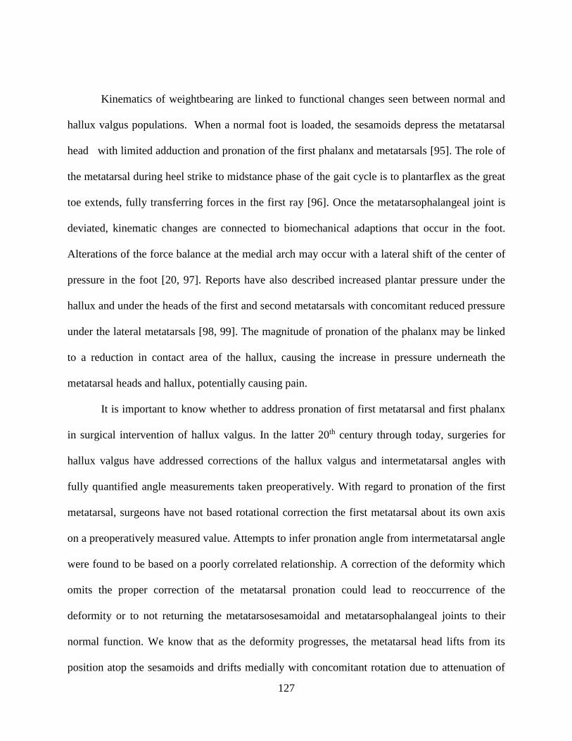
127
Kinematics of weightbearing are linked to functional changes seen between normal and
hallux valgus populations. When a normal foot is loaded, the sesamoids depress the metatarsal
head with limited adduction and pronation of the first phalanx and metatarsals [95]. The role of
the metatarsal during heel strike to midstance phase of the gait cycle is to plantarflex as the great
toe extends, fully transferring forces in the first ray [96]. Once the metatarsophalangeal joint is
deviated, kinematic changes are connected to biomechanical adaptions that occur in the foot.
Alterations of the force balance at the medial arch may occur with a lateral shift of the center of
pressure in the foot [20, 97]. Reports have also described increased plantar pressure under the
hallux and under the heads of the first and second metatarsals with concomitant reduced pressure
under the lateral metatarsals [98, 99]. The magnitude of pronation of the phalanx may be linked
to a reduction in contact area of the hallux, causing the increase in pressure underneath the
metatarsal heads and hallux, potentially causing pain.
It is important to know whether to address pronation of first metatarsal and first phalanx
in surgical intervention of hallux valgus. In the latter 20th century through today, surgeries for
hallux valgus have addressed corrections of the hallux valgus and intermetatarsal angles with
fully quantified angle measurements taken preoperatively. With regard to pronation of the first
metatarsal, surgeons have not based rotational correction the first metatarsal about its own axis
on a preoperatively measured value. Attempts to infer pronation angle from intermetatarsal angle
were found to be based on a poorly correlated relationship. A correction of the deformity which
omits the proper correction of the metatarsal pronation could lead to reoccurrence of the
deformity or to not returning the metatarsosesamoidal and metatarsophalangeal joints to their
normal function. We know that as the deformity progresses, the metatarsal head lifts from its
position atop the sesamoids and drifts medially with concomitant rotation due to attenuation of

128
the collateral ligaments at the metatarsophalangeal joint [23]. Yet, traditional imaging used
within clinical settings for diagnosis and surgical planning focuses on first phalanx adduction,
first metatarsal abduction and sesamoid subluxation. Any attempts to view the phalanx and
metatarsal pronation clinically in coronal plane images are taken from plain film x-ray, which
may vary with the quality of roentgenography, may distort the view of the bone due to projection
onto a plane and may be dependent on the orientation of the x-ray cassette. Our findings indicate
the first metatarsal rotates outward from the normal position with respect to second metatarsal as
the deformity emerges. The 8° difference in pronation found here suggests surgical intervention
of this malrotation may be needed alongside existing correction of the sesamoid complex to
return the joint to its normal functioning state. Furthermore, our results indicate a significant
difference occurred in the pronation of the first phalanx relative to the first metatarsal between
the Normal and HV subject groups. We found the first phalanx pronated over 15 degrees
between hallux valgus’ and normals. This level of migration of the phalanx may indicate the
need to correct ligament laxity in the metatarsophalangeal joint as the instability, caused by
attenuated ligaments, permitting the phalanx deviation. Surgical algorithms developed for HV
correction may need the new information found in this study.
Our study is comparable with others in the literature. With respect to the methodology,
our work is similar to efforts by Ledoux et. al. establishing a computational algorithm to define
foot alignment based on computed orientation of bones in the foot [42]. With regard to reported
pronation, results from Collan et al. are comparable. Collan reported average first metatarsal
pronation of 8±2 and 2±13 degrees for hallux valgus and normal patients respectively. In
contrast to the work by Eustace, we did not find a strong relationship of IMA and pronation.

129
From a methods standpoint, we believe a more repeatable and reliable method is necessary to
obtain comprehensive analysis of orientation. Our method does not rely on imaging from a
particular angle or having the foot oriented in a particular manner. Our results directly compared
the orientations of the first metatarsal to the first phalanx and to the second metatarsal and could
be computed from any CT image. However, the technique is mathematically intensive and not
quickly obtained clinically. A simple clinical measure of the true pronation remains to be
determined.
This investigation has some limitations. Our study used a weight bearing device added to
a standard horizontal CT and relied on voluntary patient participation because the imaging was
not the standard of care. Replication of this study is dependent on using the same rotation
sequence put forth here to calculate “Cardan angles”. We used the recommendations of the
International Society of Biomechanics.
9.2 INFERENCES FROM THE DENSITY RESULTS
This study is the first to examine the in vivo density profile of both normals and hallux valgus
patients. We first found a decreased density on the lateral sides of the metatarsal base in HV
patients compared to normals. We also found differences in the medial/lateral and dorsal/plantar
densities within the normal and HV groups. A decreased density in HV patients occurred in both
the plantar and dorsal regions of the metatarsal base. This study demonstrates the impact of HV
foot malformations beyond visible geometric changes. It is understood that the loading of the
130
first metatarsal is altered because of HV [97, 100]. The differences in bone densities between
groups indicate a shift in mechanical loading at the tarsometatarsal due to hallux valgus. The
tarsometatarsal joint facilitates load transmission from the midfoot to the forefoot, transferring
weight from the ankle to the toes.
The density profiles in the forefoot and midfoot provide evidence that may be linked to
the mechanical load history and propagation of forces within the foot. It is reasonable that
changes in bone alignment alter the transmission of forces and then leads to bony remodeling. It
is understood that in normal feet, the most medial and lateral tarsometatarsals help facilitate the
transmission of the forces, most notably at the first tarsometatarsal during inversion and eversion
of the foot [101]. A study by Lakin et al. of normal feet tested the whole foot under increased
mechanical loads with varied foot positions and showed a greater increase in contact area at the
first and fifth tarsometatarsal joints compared to the other tarsometatarsal joints. During the onset
of HV, adaptions to load, variations in foot position and transmission of forces in the midfoot
remain unknown. However, density changes are evidence that force transmission is altered due
to the deformity. In our HV group, we found similar densities on the medial and lateral sides of
the metatarsal base, a result that contrasts with the density pattern of the normal feet (p<0.05).
The adducted metatarsal might unload the lateral side of the metatarsal base, which could lead to
the changes seen in these results. An adducted metatarsal may also lead to ligamentous laxity on
the lateral side of the proximal metatarsal causing the reduced density.
The stability of the joint could relate to the differences in density. Laxity at the joints
[21, 96] and the shapes of the bones [102] were found to play roles in the propagation of the
forces through the midfoot. We found reduced density at the medial and lateral regions at the
metatarsal base between normal and HV groups. Obliquity [103, 104] and ligament laxity on the

131
lateral side [9] of the TMT have been linked to the progression of HV. In work on the proximal
metatarsal articular surface, ElSaid suggested lateral deviation might predispose the joint to HV.
Work by Mason on the proximal metatarsal suggested stability at the tarsometatarsal joint was
dependent on the shape of the articular surface. Mason found the number of distinct facets in the
normal group (3 facets) was reduced in the HV group (1 facet). We found a significant change in
density between groups on the lateral metatarsal base, evidence supporting the ideas of both
studies. In addition, Mason found that the lateral plantar prominence near the peroneus longus
tubercle, was diminished in the HV group. This finding suggests that HV destabilizes normal
loading of the tarsometatarsal joint, resulting in changes in the cuneiform. Our findings, reduced
density in the lateral region and no change at the medial region of the cuneiform, although
without statistical significance, show the internal loading changes may manifest in the form of
density changes.
Previous studies of density in the first ray have used cadaveric specimens to which the
current results can be compared. Muehleman reported the dorsal and lateral regions of the
metatarsal were more dense than the plantar (0.091 g/cm2 larger) and medial (0.071 g/cm2 larger)
regions, in agreement with our findings in the normal group. Across the base of the metatarsal,
Coskun found the lateral region of the metatarsal was more dense than the medial, a contrast to
our findings of the greater density in the medial region. In the cuneiform, Coskun found the
bone was more dense laterally than medially, a finding that agreed with the density differences of
the normal group in this study. In healthy in vivo participants, Panchbhavi found results similar
to ours at the proximal medial cuneiform, in that the dorsal region was more dense than plantar.
When comparing lateral to medial, Panchbhavi found both sides to be of similar density in the
plantar region and we found no differences overall in both the normal and HV groups.

132
While this study is unique, some limitations should be considered. First, our study was
conducted without a phantom with a known density. Therefore, we cannot report the absolute
density of bone. Furthermore, our study sample size was small. The patient population also
presented a potential limitation because HV occurs in the general population in two groups:
acquired and congenital. However, we did not distinguish between the two populations in this
study.
9.3 INFERENCES OF FEA MODELING RESULTS
The metatarsosesamoidal modeling work shown here is the first finite element undertaking to
explore the interaction at the contact of the sesamoids and metatarsal head. Our patient specific
forefoot models were loaded with force magnitudes equivalent to standing. The
metatarsosesamoidal model was configured to represent the cartilage in contact with the base of
the metatarsal head. Ligaments around the joint were modeled as springs to govern the motion
of the sesamoids. Our findings showed at lower loads, the average contact pressures at the
metatarsal head were similar in both models of hallux valgus and normal subjects. However, at
larger sesamoid load, we found an increase in the average contact pressure of both models. The
average contact pressure of the HV model was nearly 2 MPa and the normal model was 1.25
MPa. The increase in pressure corresponded with an increased in contact force at the metatarsal
head where it was calculated in normal and HV models as 43 N and 63 N respectively. We found
the lateral sesamoid in the HV model makes minimal contact with the metatarsal and thus does

133
little to support weightbearing while standing. This demonstrates the added responsibility of the
weightbearing in the medial sesamoid of HV model leads to an increase in contact pressure and
contact force at the metatarsal.
Hallux valgus alters the mechanics of contact between the metatarsal and sesamoids. In a
normal foot, the sesamoids track and move within small grooves, known as the medial and
lateral trochlea that are separated by the crista. The deformity shifts the position of the medial
sesamoid from the medial metatarsal to the central region of the metatarsal head. We found
increased contact pressure in both models as loading increased with the HV model having higher
average and peak contact stress at 80N of applied sesamoid load. Clinically, HV can wear away
the crista due to the shifting of the region of the contact between the metatarsal and medial
sesamoid. Due to smoothing during model creation or potentially crista wearing in the patient
used for the HV model, this modeling effort represents a best case scenario between the contact
of the sesamoid and metatarsal because the ridge forming the crista is not included in this FEA
model. In a case of moderate HV where the crista is present and causing pain, the ridge
contacting the medial sesamoid would increase average contact pressure and contact force. The
pronation of the metatarsal concomitantly forces the lateral sesamoid to lose much of its contact
with the lateral metatarsal, as the abductor and adductor hallucis remain intact and restrain
sesamoidal movement. The average contact area of the medial sesamoids in both models
increased as input force increased and did not differ between the normal and HV models across
the loading cycle. But that relationship was not found in the lateral sesamoids of both models.
We found the average contact pressure, force, and area of the lateral sesamoid in the normal
model were vastly larger than that of the lateral sesamoid in the HV model. Without an increase

134
of contact area in the medial sesamoid of the HV model, the average contact pressure and
average contact force increased.
The sensitivity analysis was used to explore the contact pressure at the sesamoid under
modified cartilage modulus of elasticity. The simulations of modified cartilage elasticity
modulus yielded increases in contact pressure, with a maximum average contact pressure found
at 90% E. At the medial sesamoid, both modified cartilage values produced average contact
pressures that surpassed 2 MPa under the greatest load input for both HV and normal models. It
has been documented that excessive loading can be detrimental to the articular cartilage altering
its function and behavior. Repeated impact loading at 5 MPa was shown to cause time
dependent changes similar to OA and cell death in cartilage via decreases in chondrocytes [105-
107]. In our study, the results from our sensitivity analysis show stress in the cartilage did not
approach 5 MPa, therefore we cannot conclude our HV model produced loading that leads to
cartilage degeneration. But, when the crista is present in a model of an HV foot and in contact
with the medial sesamoid, it could produce contact pressures greater than what was found here in
this model.
The modeling shown in this dissertation demonstrated the mechanical response at the
metatarsosesamoidal joint during standing. Many previous finite element modeling studies of the
foot have included the sesamoids as bodies merged into the metatarsal and not distinct bones
attached to the metatarsal by ligaments. The results of the studies report plantar soft tissue
pressures during standing and gait. Therefore, our model is not comparable due to a lack of
reporting plantar pressure on the metatarsal head at the metatarsosesamoidal joint. Two studies
have reported stress in bone of the metatarsal. At the midstance phase of the gait cycle, Chen
reported maximum von Mises stress of approximately 1 MPa, but the location of the peak was
135
not reported [108]. Cheung computed plantar stress during standing and reported peak von Mises
stress of 2.3 MPa in the first metatarsal but gave no indication of the specific location in the bone
[64]. Both models excluded the sesamoids. We found a peak von Mises stress of over 3.5 MPa
in the metatarsal head at a maximum loading, which is greater than the peak values found by
Chen and Cheung.
Studies have reported plantar pressure underneath the first metatarsal during one legged
standing, two legged standing and over the gait cycle. While these efforts are very valuable to
understanding loading in various regions of the foot, they do not directly address loading at the
interface of the sesamoids and metatarsal head. Clinical manifestations of OA in the plantar
aspects of the metatarsal, particularly at the crista and medial facet of the metatarsal head, have
been reported [109]. It is important that we understand loading of the metatarsal and only direct
measurement can be used to determine stress at the metatarsosesamoidal joint. Our model
allowed us to report the contact pressure and forces in that region to determine differences in the
magnitude of loading in patients with HV compared to normals at the metatarsal head. Estimates
of plantar pressure at the metatarsal head have not been reported due to a lack of technology for
direct pressure measurements. But, the plantar pressure measurements can provide initial
conditions for finite element modeling. Cavanagh and Weijers have each reported plantar
pressure measured while patients with normal feet stood in place, while Jonely reported plantar
pressure from one legged standing. The range of reported plantar pressure at the metatarsal head
was between 35 and 80 kPa. Weijers reported pressure under the sesamoid, which they found to
be 80 kPa. The plantar pressure of HV patients was measured by Martinez-Nova and Koller
during the gait cycle and found to be close to 340 kPa and 350 kPa respectively. We believe our

136
loading conditions, up to 80 N over ~175 mm2 surface area, spanned the reported loading
magnitudes and thus our results reflect physiologically realistic loads on the proximal metatarsal.
Our patient specific tarsometatarsal models were loaded with force magnitudes
equivalent to standing. The models were tested and validated to ensure the results reflected
anatomic motion of the first metatarsal while under load. In the normal model, the loading
produced a smaller intermetatarsal angle, while in the HV model loading increased the
intermetatarsal angle. Very little is known about loading of the TMT in patients with hallux
valgus and to this point, no FEA models of the joint with HV have been reported. We were able
to show that the average contact pressure in the cuneiform of both the HV and normal models
were similar. We found differences at the metatarsal base, where the average contact pressures
in the normal model were 75% larger than that of the HV model at lower loads and 20% larger at
higher loads. Our results show a difference in loading profile of the metatarsal base and
cuneiform in the HV and normal models. In general, we found the average contact pressures and
forces in the normal model were greater in the metatarsal base than in the cuneiform. That was
reversed in the HV model where the average contact pressures and forces were greater in the
cuneiform. Internally, our path lines provide a tool to compare cuneiform pressures of both
models in the mediolateral and dorsoplantar directions. We believe HV can lead to changes in
loading due to the medial deviation of the first metatarsal. In the normal model, we found higher
stress on the lateral and dorsal sides compared to the medial and plantar sides. In the HV model
we found lower stress and a different stress profile. In outer regions of the cuneiform, we found
similar densities comparing medial to lateral and dorsal to plantar. In the central region, we
found higher stress medially and plantarly which represents a shift from the results of the normal
model.

137
The function of the tarsometatarsal joint is to provide stability to the midfoot and
forefoot. Contact pressure at the tarsometatarsal has only been previously reported
experimentally. An in vitro biomechanical test of a normal foot by Lakin reported contact
pressure and contact force. Using pressure sensitive film, Lakin and colleagues compressively
loaded a normal foot through the tibia over a range of force inputs equivalent to half bodyweight,
bodyweight and twice bodyweight. They found the contact pressure increased from 1 MPa to 2
MPa at the largest compressive load. We did not find good agreement with their reported
contact pressure. We found that the average contact pressure was below 0.6 MPa. The
differences can be related to two factors influencing the outcomes of both studies. First, the
loading condition between the two studies differed greatly. We did not load whole foot in our
model and whole bodyweight load. Second, Lakin et al. utilized pressure film to measure
contact at the tarsometatarsal joint. The type of film used in the study was not able to register
loads below 0.5 MPa. Our study had no such threshold and we found the majority of the nodes
used to calculate the contact pressure were below 0.49 MPa. As a result, our average contact
pressure was lower than Lakin, while the contact area was much larger. In the case of both
studies, ours and Lakin et al., the contact forces were calculated directly from the pressure and
area and do not have agreement. We found the contact force to be twice as larger as reported by
Lakin et al. The behavior of the joint, with linearly increasing contact pressure and input load,
was in agreement between the studies.
Previous finite element [110] and musculoskeletal [111] and static calculation [112]
models have described loading across the tarsometatarsal joint. No consensus has been reached
on the loading at the tarsometatarsal joint, with loads during gait reported to be 0.67 to 1.40
times body weight. We did use loading conditions that approach the midstance and toe-off as

138
the previous authors described, therefore we do not expect agreement here. As the foot moves
from a static standing position to a more dynamic position of mid-stance and toe off, the loads in
the foot will increase. Wang and Niu reported von Mises stress distributions at the
tarsometatarsal joint during midstance [113, 114]. Both papers lack specific information about
peak loading at the tarsometatarsal. Niu included figures of von Mises stress at the cuneiform of
a normal foot. Their findings show a wide stress distribution of approximately 1 MPa, which is
in more agreement with our own findings.
The results and conclusion from our modeling are not without some limitations to be
considered. Both models have ligaments modeled as spring elements. Many published FEA
models contain ligaments represented as a solid elastic 3D body. During the segmentation
process, we were not able to view tendon and ligaments in the CT scans. Therefore, we could
not create 3D ligaments. The behavior of the ligaments is tension only and has been modeled as
tension only in many cases. Our model was having difficulty converging with tension only
ligaments so we included a small stiffness in compression to obtain a converging solution.
Additionally, because we were unable to view cartilage in our CT scans, we modeled the
thickness of the cartilage as uniform and this may not be the vase in the sesamoid, metatarsal
base and cuneiform of the normal and HV patients.

139
10.0 CONCLUSIONS
This study reported very important clinical and biomechanical results regarding the hallux valgus
deformity. Our clinical findings of pronation angle in HV and normal patients have an immediate
impact on surgical planning for the correction of the HV deformity. Our study emphasized that
pronation is an important factor in the morphology of hallux valgus. We found a variation of
8.6° in pronation of the first metatarsal between foot groups and a statistically significant
difference of 14.5° in first phalanx pronation between foot groups. Surgeries are designed to
correct HV deformity and reduce pain, but may leave malrotation unaddressed. Our results
provide evidence to encourage consideration of pronation in surgical planning. Future work
should possibly address surgical techniques to fully correct the HV deformity.
Our clinical findings of a shift in the densitometric profile of the HV group compared to
the normal group are important when considering how HV progresses over time. It was the first
in vivo study to compare the densitometric profile of the tarsometatarsal joint in HV patients. The
load history of HV patients is currently unknown with no published investigations. Local bone
density has the potential to indicate bone tissue history. It is important to the study of HV to
determine how the deformity affects the tarsometatarsal joint. Future clinical imaging work
should address the ligamentous laxity in the first ray of HV patients.

140
Our finite element modeling effort produced a better understanding of the mechanics at
the metatarsosesamoidal and tarsometatarsal joints due to hallux valgus. We found increased
pressure on the metatarsal head due to a shift in the position of the sesamoid contact. Moving
forward, subsequent studies can use this dissertation as a starting point to better understand
loading difference found in patients with hallux valgus as compared the normal population. The
sensitivity of the simple ligament modeling done here should be advanced such that the three
joints of the first ray (metatarsosesamoidal, metatarsophalangeal, and tarsometatarsal) can be
included in a single model to replicate more natural positions during standing and gait. As well,
modeling the joints together will demonstrate how one joint influences the mechanics at the other
joints.

141
APPENDIX A
MATLAB CODE
The following code was used to calculate the contact area and contact force from the ANSYS
contact pressure shown in the Results section.
function ContactAnalysis2017 % Bradley C. Campbell % January 2017 % FEA Output Processing Code close all;clc;clear all; % InputData = 'D:\BCampbellFEA_Results\TMT\Normal\Trial3_03132017'; % InputData = 'D:\BCampbellFEA_Results\TMT\HV\Trial2_03142017'; InputData = 'D:\BCampbellFEA_Results\HV\CartilageSensty\HVCartilage_80N_Ramped_025Mesh_03082017'; addpath(genpath(InputData)); cd(InputData) % 1 - Lateral % 2 - Medial % MTS Contact and Target Input Cont1=fopen('LateralSesContactElementsContacts.txt','r'); Cont2=fopen('MedialSesContactElementsContacts.txt','r');

142
Tar1=fopen('LateralSesContactElementsTargets.txt','r'); Tar2=fopen('MedialSesContactElementsTargets.txt','r'); f=fopen('ContactPressureTime6.txt','r'); g=fopen('NodeCoords.txt','r'); h=fopen('DispCoordTime6.txt','r'); % TMT Contact and Target %{ Cont1=fopen('MetContactElementsContact.txt','r'); Cont2=fopen('CunContactElementsContact.txt','r'); Cont3=fopen('CartilageContactElementsContact.txt','r'); Tar1=fopen('MetContactElementsTarget.txt','r'); Tar2=fopen('CunContactElementsTarget.txt','r'); Tar3=fopen('CartilageContactElementsTarget.txt','r'); f=fopen('ContactPressureTime9.txt','r'); g=fopen('NodeCoords.txt','r'); h=fopen('DispCoordTime9.txt','r'); %} x=0; while (~feof(Cont1)) if x == 0 hd=textscan(Cont1,'%s',1,'HeaderLines',9); x1=cell2mat(textscan(Cont1,'%n %n %n %n %n %n %n %n %n %n %n %n %n')); %C_Node = x1; % The format of the ###.txt inadvertently adds a row with -1...delete C_Node1 = x1(1:end,:); else hd=textscan(Cont1,'%s',1,'HeaderLines',1); x1=cell2mat(textscan(Cont1,'%n %n %n %n %n %n %n %n %n %n %n %n %n')); %C_Node = [C_Node; x1]; C_Node1 = [C_Node1; x1(1:end,:)]; end x=x+1; end ContElem1(:,1) = C_Node1(:,1); ContElem1(:,2:9) = C_Node1(:,6:13); fclose(Cont1); x=0; while (~feof(Tar1)) if x == 0 hd=textscan(Tar1,'%s',1,'HeaderLines',9); x1=cell2mat(textscan(Tar1,'%n %n %n %n %n %n %n %n %n %n %n %n %n')); %T_Node = x1; % The format of the ###.txt inadvertently adds a row with -

143
1...delete T_Node1 = x1(1:end,:); else hd=textscan(Tar1,'%s',1,'HeaderLines',1); x1=cell2mat(textscan(Tar1,'%n %n %n %n %n %n %n %n %n %n %n %n %n')); %T_Node = [T_Node; x1]; T_Node1 = [T_Node1; x1(1:end,:)]; end x=x+1; end TarElem1(:,1) = T_Node1(:,1); TarElem1(:,2:9) = T_Node1(:,6:13); fclose(Tar1); x=0; while (~feof(Cont2)) if x == 0 hd=textscan(Cont2,'%s',1,'HeaderLines',9); x1=cell2mat(textscan(Cont2,'%n %n %n %n %n %n %n %n %n %n %n %n %n')); %C_Node = x1; % The format of the ###.txt inadvertently adds a row with -1...delete C_Node2 = x1(1:end,:); else hd=textscan(Cont2,'%s',1,'HeaderLines',1); x1=cell2mat(textscan(Cont2,'%n %n %n %n %n %n %n %n %n %n %n %n %n')); %C_Node = [C_Node; x1]; C_Node2 = [C_Node2; x1(1:end,:)]; end x=x+1; end ContElem2(:,1) = C_Node2(:,1); ContElem2(:,2:9) = C_Node2(:,6:13); fclose(Cont2); x=0; while (~feof(Tar2)) if x == 0 hd=textscan(Tar2,'%s',1,'HeaderLines',9); x1=cell2mat(textscan(Tar2,'%n %n %n %n %n %n %n %n %n %n %n %n %n')); %T_Node = x1; % The format of the ###.txt inadvertently adds a row with -1...delete T_Node2 = x1(1:end,:); else hd=textscan(Tar2,'%s',1,'HeaderLines',1); x1=cell2mat(textscan(Tar2,'%n %n %n %n %n %n %n %n %n %n %n %n %n')); %T_Node = [T_Node; x1]; T_Node2 = [T_Node2; x1(1:end,:)];

144
end x=x+1; end TarElem2(:,1) = T_Node2(:,1); TarElem2(:,2:9) = T_Node2(:,6:13); fclose(Tar2); % x = 0; % while (~feof(Cont3)) % if x == 0 % hd=textscan(Cont3,'%s',1,'HeaderLines',9); % x1=cell2mat(textscan(Cont3,'%n %n %n %n %n %n %n %n %n %n %n %n %n')); % %C_Node = x1; % The format of the ###.txt inadvertently adds a row with -1...delete % C_Node3 = x1(1:end,:); % else % hd=textscan(Cont3,'%s',1,'HeaderLines',1); % x1=cell2mat(textscan(Cont3,'%n %n %n %n %n %n %n %n %n %n %n %n %n')); % %C_Node = [C_Node; x1]; % C_Node3 = [C_Node3; x1(1:end,:)]; % end % x=x+1; % end % ContElem3(:,1) = C_Node3(:,1); ContElem3(:,2:9) = C_Node3(:,6:13); % fclose(Cont3); % % x=0; % while (~feof(Tar3)) % if x == 0 % hd=textscan(Tar3,'%s',1,'HeaderLines',9); % x1=cell2mat(textscan(Tar3,'%n %n %n %n %n %n %n %n %n %n %n %n %n')); % %T_Node = x1; % The format of the ###.txt inadvertently adds a row with -1...delete % T_Node3 = x1(1:end,:); % else % hd=textscan(Tar3,'%s',1,'HeaderLines',1); % x1=cell2mat(textscan(Tar3,'%n %n %n %n %n %n %n %n %n %n %n %n %n')); % %T_Node = [T_Node; x1]; % T_Node3 = [T_Node3; x1(1:end,:)]; % end % x=x+1; % end % TarElem3(:,1) = T_Node3(:,1); TarElem3(:,2:9) = T_Node3(:,6:13); % fclose(Tar3);

145
% Results Files Input pressure = []; while (~feof(f)) if x == 0 x1=cell2mat(textscan(f,'%n %n %n %n %n %n %n %n %n %n %n','headerlines',9)); pressure = x1; else x1=cell2mat(textscan(f,'%n %n %n %n %n %n %n %n %n %n %n','headerlines',1)); pressure = [pressure; x1]; end x=x+1; end % read node data x=0; while (~feof(g)) hd=textscan(g,'%s',4); x1=cell2mat(textscan(g,'%n %n %n %n')); if x==0 node=x1; else node=[node;x1]; end x=x+1; end x=0; while (~feof(h)) if x == 0 x1=cell2mat(textscan(h,'%n %n %n %n %n','headerlines',9)); disp= x1; else x1=cell2mat(textscan(h,'%n %n %n %n %n','headerlines',1)); disp = [disp; x1]; end x=x+1; end fclose(f);fclose(g); fclose(h);

146
% MTS Models [MedSesContForce, MedSesContArea, MedSesAvgContPress] = contarea(ContElem2, node, pressure) [MedSesTarForce, MedSesTarArea, MedSesAvgTarPress] = contarea(TarElem2, node, pressure); [LatSesTarForce, LatSesTarArea, LatSesAvgTarPress] = contarea(TarElem1, node, pressure); [LatSesContForce, LatSesContArea, LatSesAvgContPress] = contarea(ContElem1, node, pressure) % TMT Models % [MetContForce, MetContArea, MetAvgContPress] = contarea(ContElem1, node, pressure) % [CunContForce, CunContArea, CunAvgContPress] = contarea(ContElem2, node, pressure) % [CartContForce, CartContArea, CartAvgContPress] = contarea(ContElem3, node, pressure) % Lakin Comparison x = 1; for i = 1:length(pressure) if pressure(i,4) > 0.5 LakinPress(x,1) = pressure(i,1); LakinPress(x,4) = pressure(i,4); x = x+1; end end [LakinCartContForce, LakinCartContArea, LakinCartAvgContPress] = contarea(ContElem3, node, LakinPress) end % ContElem - All elements in the contact [element# node1...node8] function [AvgContForce, AvgContArea,ContPress] = contarea(ContElem, NodeCoords, NodePress) CNodePress(:,1) = NodePress(:,1); CNodePress(:,2) = NodePress(:,4); clear NodePress CEleNodes = ContElem(:,2:9); [n, m] = size(CEleNodes); SubArea = zeros(n,1); for i = 1:n NodeNums = CEleNodes(i,:); if isnan(NodeNums) == 1 i = i+1; NodeNums = CEleNodes(i,:); end % P1=CEleNodes(i,1); P2=CEleNodes(i,2); P3=CEleNodes(i,3);

147
P4=CEleNodes(i,4); % P5=CEleNodes(i,5); P6=CEleNodes(i,6); P7=CEleNodes(i,7); P8=CEleNodes(i,8); %Pull Coordinates P1(1:3) = NodeCoords(find(NodeNums(1)==NodeCoords(:,1)),2:4); P2(1:3) = NodeCoords(find(NodeNums(2)==NodeCoords(:,1)),2:4); P3(1:3) = NodeCoords(find(NodeNums(3)==NodeCoords(:,1)),2:4); P4(1:3) = NodeCoords(find(NodeNums(4)==NodeCoords(:,1)),2:4); P5(1:3) = NodeCoords(find(NodeNums(5)==NodeCoords(:,1)),2:4); P6(1:3) = NodeCoords(find(NodeNums(6)==NodeCoords(:,1)),2:4); P7(1:3) = NodeCoords(find(NodeNums(7)==NodeCoords(:,1)),2:4); P8(1:3) = NodeCoords(find(NodeNums(8)==NodeCoords(:,1)),2:4); t1a=P8-P1; t1b=P8-P5; A(1)=1/2*norm(cross(t1a,t1b)); t2a=P8-P5; t2b=P8-P2; A(2)=1/2*norm(cross(t2a,t2b)); t3a=P8-P2; t3b=P8-P6; A(3)=1/2*norm(cross(t3a,t3b)); t4a=P8-P6; t4b=P8-P3; A(4)=1/2*norm(cross(t4a,t4b)); t5a=P8-P3; t5b=P8-P7; A(5)=1/2*norm(cross(t5a,t5b)); t6a=P8-P7; t6b=P8-P4; A(6)=1/2*norm(cross(t6a,t6b)); SubArea(i,1) = sum(A); %Pull Nodal Pressure CP1 = CNodePress(find(NodeNums(1)==CNodePress(:,1)),2); if isempty(CP1) CP1 = 0; end CP2 = CNodePress(find(NodeNums(2)==CNodePress(:,1)),2); if isempty(CP2) CP2 = 0; end CP3 = CNodePress(find(NodeNums(3)==CNodePress(:,1)),2); if isempty(CP3) CP3 = 0; end CP4 = CNodePress(find(NodeNums(4)==CNodePress(:,1)),2); if isempty(CP4) CP4 = 0; end CP5 = CNodePress(find(NodeNums(5)==CNodePress(:,1)),2); if isempty(CP5) CP5 = 0; end CP6 = CNodePress(find(NodeNums(6)==CNodePress(:,1)),2); if isempty(CP6) CP6 = 0; end

148
CP7 = CNodePress(find(NodeNums(7)==CNodePress(:,1)),2); if isempty(CP7) CP7 = 0; end CP8 = CNodePress(find(NodeNums(8)==CNodePress(:,1)),2); if isempty(CP8) CP8 = 0; end p1a=(CP8+CP1+CP5)/3; p2a=(CP8+CP5+CP2)/3; p3a=(CP8+CP2+CP6)/3; p4a=(CP8+CP6+CP3)/3; p5a=(CP8+CP3+CP7)/3; p6a=(CP8+CP7+CP4)/3; Pressures(i,:) = [CP1 CP2 CP3 CP4 CP5 CP6 CP7 CP8]; Force(1) = A(1)*p1a; Force(2) = A(2)*p2a; Force(3) = A(3)*p3a; Force(4) = A(4)*p4a; Force(5) = A(5)*p5a; Force(6) = A(6)*p6a; ForceArea(i,1) = sum(Force); ForceArea(i,2) = sum(A); clear CP NoMidsForce(i,1) = sum(A)*(CP1+CP2+CP3)/3; end x = 1; for i = 1:length(ForceArea) if ForceArea(i,1) ~= 0 ContForce(x,1) = ForceArea(i,1); ContArea(x,1) = ForceArea(i,2); x = x+1; end end % Check and see if nodes M, N and P are zero if sum(Pressures(:,5)) == 0 && sum(Pressures(:,6)) == 0 && sum(Pressures(:,8)) == 0 AvgContForce = sum(NoMidsForce); else AvgContForce = sum(ContForce); end AvgContArea = sum(ContArea); ContPress = AvgContForce/AvgContArea ; end %Separate the Non-Zero Force and Area Pairs % Ave_ContPress = sum(ForceArea(:,1))/sum(ForceArea(:,2));

149
BIBLIOGRAPHY
1. Dolinis, J., J.E. Harrison, and G.R. Andrews, Factors associated with falling in older
Adelaide residents. Aust N Z J Public Health, 1997. 21(5): p. 462-8.
2. Menz, H.B. and M.E. Morris, Footwear characteristics and foot problems in older
people. Gerontology, 2005. 51(5): p. 346-51.
3. Hockenbury, R.T., Forefoot problems in athletes. Med Sci Sports Exerc, 1999. 31(7
Suppl): p. S448-58.
4. Nix, S., M. Smith, and B. Vicenzino, Prevalence of hallux valgus in the general
population: a systematic review and meta-analysis. J Foot Ankle Res, 2010. 3: p. 21.
5. Bonney, G. and I. Macnab, Hallux valgus and hallux rigidus; a critical survey of
operative results. J Bone Joint Surg Br, 1952. 34-B(3): p. 366-85.
6. Wulker, N. and F. Mittag, The treatment of hallux valgus. Dtsch Arztebl Int, 2012.
109(49): p. 857-67; quiz 868.
7. Saxena, A., Special procedures in foot and ankle surgery. 2013, London: Springer. xii,
350 pages.
8. Coughlin, M.J. and F.M. Thompson, The high price of high-fashion footwear. Instr
Course Lect, 1995. 44: p. 371-7.
9. Coughlin, M.J., Hallux valgus. J Bone Joint Surg Am, 1996. 78(6): p. 932-66.
10. Lagaay, P.M., et al., Rates of revision surgery using Chevron-Austin osteotomy, Lapidus
arthrodesis, and closing base wedge osteotomy for correction of hallux valgus deformity.
J Foot Ankle Surg, 2008. 47(4): p. 267-72.
11. Kilmartin, T.E., Revision of failed foot surgery: a critical analysis. J Foot Ankle Surg,
2002. 41(5): p. 309-15.
12. Menz, H.B., M.F. Gilheany, and K.B. Landorf, Foot and ankle surgery in Australia: a
descriptive analysis of the Medicare Benefits Schedule database, 1997-2006. J Foot
Ankle Res, 2008. 1(1): p. 10.

150
13. Menz, H.B., et al., Impact of hallux valgus severity on general and foot-specific health-
related quality of life. Arthritis Care Res (Hoboken), 2011. 63(3): p. 396-404.
14. Conti, S.F., Muriuki, M., Miller, M.C., The Relative Bone Density at the Tarsometatarsal
Joint in Hallux Valgus, A.G.H.O. University of Pittsburgh, Editor. 2010.
15. Mann, R.A. and M.J. Coughlin, Hallux valgus--etiology, anatomy, treatment and surgical
considerations. Clin Orthop Relat Res, 1981(157): p. 31-41.
16. Perera, A.M., L. Mason, and M.M. Stephens, The pathogenesis of hallux valgus. J Bone
Joint Surg Am, 2011. 93(17): p. 1650-61.
17. Kelikian, A.S., S.K. Sarrafian, and S.K. Sarrafian, Sarrafian's anatomy of the foot and
ankle : descriptive, topographical, functional. Third Edition. ed. 2011, Philadelphia:
Wolters Kluwer Health/Lippincott Williams & Wilkins. xix, 759 pages.
18. Currey, J.D., Bones : structure and mechanics. 2002, Princeton, NJ: Princeton University
Press. xii, 436 p.
19. Yildirim, Y., et al., Effect of metatarsophalangeal joint position on the reliability of the
tangential sesamoid view in determining sesamoid position. Foot Ankle Int, 2005. 26(3):
p. 247-50.
20. Arinci Incel, N., et al., Muscle imbalance in hallux valgus: an electromyographic study.
Am J Phys Med Rehabil, 2003. 82(5): p. 345-9.
21. Robinson, A.H. and J.P. Limbers, Modern concepts in the treatment of hallux valgus. J
Bone Joint Surg Br, 2005. 87(8): p. 1038-45.
22. Hansen, John T., Bruce M. Koeppen, and Bruce M. Koeppen. Netter's Atlas of Human
Physiology. 2002. Teterbobo, New Jersey: Elsevier Inc, 223 p.
23. Eustace, S., et al., Radiographic features that enable assessment of first metatarsal
rotation: the role of pronation in hallux valgus. Skeletal Radiol, 1993. 22(3): p. 153-6.
24. Saltzman, C.L., et al., Coronal plane rotation of the first metatarsal. Foot Ankle Int,
1996. 17(3): p. 157-61.
25. Pelt, C.E., et al., Micro-CT Density Analysis of the Medial Wall of the Human Medial
Cuneiform. Orthopedics, 2011. 34(5): p. 363.
26. Panchbhavi, V.K., et al., CT density analysis of the medial cuneiform. Foot Ankle Int,
2013. 34(11): p. 1596-9.
27. Torkki, M., et al., Surgery vs orthosis vs watchful waiting for hallux valgus: a
randomized controlled trial. JAMA, 2001. 285(19): p. 2474-80.
151
28. Torkki, M., et al., Hallux valgus: immediate operation versus 1 year of waiting with or
without orthoses: a randomized controlled trial of 209 patients. Acta Orthop Scand,
2003. 74(2): p. 209-15.
29. Judge, M.S., et al., The effect of hallux abducto valgus surgery on the sesamoid
apparatus position. J Am Podiatr Med Assoc, 1999. 89(11-12): p. 551-9.
30. Bartel, D.L., D.T. Davy, and T.M. Keaveny, Orthopaedic biomechanics : mechanics and
design in musculoskeletal systems. Pearson Prentice Hall bioengineering. 2006, Upper
Saddle River, N.J.: Pearson/Prentice Hall. x, 370 p.
31. Weijers, R., et al., The intermetatarsal and metatarsal declination angles: geometry as a
source of error. Foot Ankle Int, 2005. 26(5): p. 387-93.
32. Eustace, S., et al., Hallux valgus, first metatarsal pronation and collapse of the medial
longitudinal arch--a radiological correlation. Skeletal Radiol, 1994. 23(3): p. 191-4.
33. Wu, G., et al., ISB recommendation on definitions of joint coordinate system of various
joints for the reporting of human joint motion--part I: ankle, hip, and spine. International
Society of Biomechanics. J Biomech, 2002. 35(4): p. 543-8.
34. Camacho, D.L., et al., A three-dimensional, anatomically detailed foot model: a
foundation for a finite element simulation and means of quantifying foot-bone position.
Journal of rehabilitation research and development, 2002. 39(3): p. 401.
35. Glasoe, W.M., et al., First ray kinematics in women with rheumatoid arthritis and bunion
deformity: a gait simulation imaging study. Arthritis Care Res (Hoboken), 2014. 66(6): p.
837-43.
36. Gutekunst, D.J., et al., Reliability of clinically relevant 3D foot bone angles from
quantitative computed tomography. Journal of Foot and Ankle Research, 2013. 6.
37. Mortier, J.P., J.L. Bernard, and M. Maestro, Axial rotation of the first metatarsal head in
a normal population and hallux valgus patients. Orthop Traumatol Surg Res, 2012.
98(6): p. 677-83.
38. Zhang, Y., et al., An in vivo study of hindfoot 3D kinetics in stage II posterior tibial
tendon dysfunction (PTTD) flatfoot based on weight-bearing CT scan. Bone Joint Res,
2013. 2(12): p. 255-63.
39. Grood, E.S. and W.J. Suntay, A joint coordinate system for the clinical description of
three-dimensional motions: application to the knee. J Biomech Eng, 1983. 105(2): p.
136-44.

152
40. Jenkyn, T.R. and A.C. Nicol, A multi-segment kinematic model of the foot with a novel
definition of forefoot motion for use in clinical gait analysis during walking. J Biomech,
2007. 40(14): p. 3271-8.
41. Yoshioka, N., et al., Weight-bearing three-dimensional computed tomography analysis of
the forefoot in patients with flatfoot deformity. J Orthop Sci, 2016. 21(2): p. 154-8.
42. Ledoux, W.R., et al., Effect of foot shape on the three-dimensional position of foot bones.
J Orthop Res, 2006. 24(12): p. 2176-86.
43. Collan, L., J.A. Kankare, and K. Mattila, The biomechanics of the first metatarsal bone in
hallux valgus: a preliminary study utilizing a weight bearing extremity CT. Foot Ankle
Surg, 2013. 19(3): p. 155-61.
44. Wolff, J., The law of bone remodelling. 1986, Berlin ; New York: Springer-Verlag. xii,
126 p.
45. Hole, K., Finite-Element Mesh Generation Methods - a Review and Classification.
Computer-Aided Design, 1988. 20(1): p. 27-38.
46. Felippa, C.A., Introduction to Finite Element Methods. 2004, University of Colorado:
Boulder, CO.
47. Brauer, J.R., What every engineer should know about finite element analysis. 2nd ed.
What every engineer should know. 1993, New York: M. Dekker. xiii, 321 p.
48. Cowin, S.C. and S.B. Doty, Tissue mechanics. 2007, New York: Springer. xvi, 682 p.
49. Bart, Z.R. and J.M. Wallace, Microcomputed tomography applications in bone and
mineral research. 2013.
50. Aarden, E.M., E.H. Burger, and P.J. Nijweide, Function of osteocytes in bone. J Cell
Biochem, 1994. 55(3): p. 287-99.
51. Hadjidakis, D.J. and Androulakis, II, Bone remodeling. Ann N Y Acad Sci, 2006. 1092:
p. 385-96.
52. Currey, J., Measurement of the mechanical properties of bone: a recent history. Clin
Orthop Relat Res, 2009. 467(8): p. 1948-54.
53. Natali, A.N. and E.A. Meroi, A review of the biomechanical properties of bone as a
material. J Biomed Eng, 1989. 11(4): p. 266-76.
54. Reilly, D.T. and A.H. Burstein, The elastic and ultimate properties of compact bone
tissue. J Biomech, 1975. 8(6): p. 393-405.

153
55. Taylor, W.R., et al., Determination of orthotropic bone elastic constants using FEA and
modal analysis. J Biomech, 2002. 35(6): p. 767-73.
56. Nakamura, S., R.D. Crowninshield, and R.R. Cooper, An analysis of soft tissue loading in
the foot--a preliminary report. Bull Prosthet Res, 1981. 10-35: p. 27-34.
57. Kopperdahl, D.L. and T.M. Keaveny, Yield strain behavior of trabecular bone. J
Biomech, 1998. 31(7): p. 601-8.
58. Linde, F., I. Hvid, and B. Pongsoipetch, Energy absorptive properties of human
trabecular bone specimens during axial compression. J Orthop Res, 1989. 7(3): p. 432-9.
59. Garcia-Aznar, J.M., et al., Load transfer mechanism for different metatarsal geometries:
a finite element study. J Biomech Eng, 2009. 131(2): p. 021011.
60. Jacob, S., et al., Stresses in a 3D two arch model of a normal human foot. Mechanics
Research Communications, 1996. 23(4): p. 387-393.
61. Garcia-Aznar, J.M., et al., Computational simulation of fracture healing: influence of
interfragmentary movement on the callus growth. J Biomech, 2007. 40(7): p. 1467-76.
62. Gefen, A., et al., Biomechanical analysis of the three-dimensional foot structure during
gait: A basic tool for clinical applications. Journal of Biomechanical Engineering-
Transactions of the Asme, 2000. 122(6): p. 630-639.
63. Gu, Y.D., et al., Foot contact surface effect to the metatarsals loading character during
inversion landing. International Journal for Numerical Methods in Biomedical
Engineering, 2011. 27(4): p. 476-484.
64. Cheung, J.T., et al., Three-dimensional finite element analysis of the foot during
standing--a material sensitivity study. J Biomech, 2005. 38(5): p. 1045-54.
65. Gomez-Benito, M.J., et al., Computational comparison of reamed versus unreamed
intramedullary tibial nails. J Orthop Res, 2007. 25(2): p. 191-200.
66. Trabelsi, N., C. Milgrom, and Z. Yosibash, Patient-specific FE analyses of metatarsal
bones with inhomogeneous isotropic material properties. J Mech Behav Biomed Mater,
2014. 29: p. 177-89.
67. Lemmon, D., et al., The effect of insoles in therapeutic footwear - A finite element
approach. Journal of Biomechanics, 1997. 30(6): p. 615-620.
68. Mow, V.C., et al., Structure and Function of Ligaments and Tendons, in Basic
orthopaedic biomechanics & mechano-biology. 2005, Lippincott Williams & Wilkins:
Philadelphia, PA. p. p. 320.

154
69. Frank, C.B., Ligament structure, physiology and function. J Musculoskelet Neuronal
Interact, 2004. 4(2): p. 199-201.
70. Mow, V.C., A. Ratcliffe, and S.L.Y. Woo, Biomechanics of diarthrodial joints. 1990,
New York: Springer-Verlag.
71. Martin, R.B., D.B. Burr, and N.A. Sharkey, Skeletal tissue mechanics. Vol. 190. 1998:
Springer.
72. Mkandawire, C., et al., Foot and ankle ligament morphometry. Journal of Rehabilitation
Research and Development, 2005. 42(6): p. 809-819.
73. Siegler, S., J. Block, and C.D. Schneck, The mechanical characteristics of the collateral
ligaments of the human ankle joint. Foot Ankle, 1988. 8(5): p. 234-42.
74. Attarian, D.E., et al., Biomechanical Characteristics of Human Ankle Ligaments. Foot &
Ankle, 1985. 6(2): p. 54-58.
75. Kura, H., et al., Mechanical behavior of the Lisfranc and dorsal cuneometatarsal
ligaments: in vitro biomechanical study. J Orthop Trauma, 2001. 15(2): p. 107-10.
76. Patil, K.M., L.H. Braak, and A. Huson, Analysis of stresses in two-dimensional models of
normal and neuropathic feet. Medical & Biological Engineering & Computing, 1996.
34(4): p. 280-284.
77. Kerin, A.J., M.R. Wisnom, and M.A. Adams, The compressive strength of articular
cartilage. Proc Inst Mech Eng H, 1998. 212(4): p. 273-80.
78. Mansour, J.M., Biomechanics of cartilage. Kinesiology: the mechanics and
pathomechanics of human movement, 2003: p. 66-79.
79. Athanasiou, K.A., et al., Biomechanical topography of human articular cartilage in the
first metatarsophalangeal joint. Clin Orthop Relat Res, 1998(348): p. 269-81.
80. Rayfield, E.J., Finite Element Analysis and Understanding the Biomechanics and
Evolution of Living and Fossil Organisms. Annual Review Earth Planetary Science 2007.
35: p. 541-76.
81. Huiskes, R. and E.Y. Chao, A survey of finite element analysis in orthopedic
biomechanics: the first decade. J Biomech, 1983. 16(6): p. 385-409.
82. Webb, J.D., S.S. Blemker, and S.L. Delp, 3D finite element models of shoulder muscles
for computing lines of actions and moment arms. Comput Methods Biomech Biomed
Engin, 2014. 17(8): p. 829-37.
155
83. Kim, S. and M. Carl Miller, Validation of a Finite Element Humeroradial Joint Model of
Contact Pressure Using Fuji Pressure Sensitive Film. J Biomech Eng, 2016. 138(1).
84. Orwoll, E.S., et al., Finite element analysis of the proximal femur and hip fracture risk in
older men. J Bone Miner Res, 2009. 24(3): p. 475-83.
85. Pena, E., et al., A three-dimensional finite element analysis of the combined behavior of
ligaments and menisci in the healthy human knee joint. J Biomech, 2006. 39(9): p. 1686-
701.
86. Wang, Y., D.W. Wong, and M. Zhang, Computational Models of the Foot and Ankle for
Pathomechanics and Clinical Applications: A Review. Ann Biomed Eng, 2015.
87. Yu, J., et al., Development of a finite element model of female foot for high-heeled shoe
design. Clin Biomech (Bristol, Avon), 2008. 23 Suppl 1: p. S31-8.
88. Budhabhatti, S.P., et al., Finite element modeling of the first ray of the foot: a tool for the
design of interventions. J Biomech Eng, 2007. 129(5): p. 750-6.
89. Spratley, E.M., et al., Validation of a population of patient-specific adult acquired
flatfoot deformity models. J Orthop Res, 2013. 31(12): p. 1861-8.
90. Gefen, A., Plantar soft tissue loading under the medial metatarsals in the standing
diabetic foot. Med Eng Phys, 2003. 25(6): p. 491-9.
91. Fuhrmann, R.A., F. Layher, and W.D. Wetzel, Radiographic changes in forefoot
geometry with weightbearing. Foot Ankle Int, 2003. 24(4): p. 326-31.
92. Shapiro, L.M. and G.E. Gold, MRI of weight bearing and movement. Osteoarthritis
Cartilage, 2012. 20(2): p. 69-78.
93. Doya, H., et al., Proposed novel unified nomenclature for range of joint motion: method
for measuring and recording for the ankles, feet, and toes. J Orthop Sci, 2010. 15(4): p.
531-9.
94. Schunke, M., E. Schulte, and U. Schumacher, Thieme atlas of anatomy. General anatomy
and musculoskeletal system. Second edition. ed. 2014, New York, New York: Thieme
Medical Publishers, Inc. xiii, 609 pages.
95. Dedmond, B.T., J.W. Cory, and A. McBryde, Jr., The hallucal sesamoid complex. J Am
Acad Orthop Surg, 2006. 14(13): p. 745-53.
96. Glasoe, W.M., H.J. Yack, and C.L. Saltzman, Anatomy and biomechanics of the first ray.
Phys Ther, 1999. 79(9): p. 854-9.
156
97. Deschamps, K., et al., The impact of hallux valgus on foot kinematics: a cross-sectional,
comparative study. Gait Posture, 2010. 32(1): p. 102-6.
98. Koller, U., et al., Plantar pressure characteristics in hallux valgus feet. J Orthop Res,
2014. 32(12): p. 1688-93.
99. Martinez-Nova, A., et al., Plantar pressures determinants in mild Hallux Valgus. Gait
Posture, 2010. 32(3): p. 425-7.
100. Wen, J., et al., Adaptive changes of foot pressure in hallux valgus patients. Gait Posture,
2012. 36(3): p. 344-9.
101. Lakin, R.C., L.T. DeGnore, and D. Pienkowski, Contact mechanics of normal
tarsometatarsal joints. J Bone Joint Surg Am, 2001. 83-A(4): p. 520-8.
102. Mason, L.W. and H. Tanaka, The first tarsometatarsal joint and its association with
hallux valgus. Bone Joint Res, 2012. 1(6): p. 99-103.
103. Easley, M.E. and H.J. Trnka, Current concepts review: hallux valgus part 1:
pathomechanics, clinical assessment, and nonoperative management. Foot Ankle Int,
2007. 28(5): p. 654-9.
104. ElSaid, A.G., et al., First metatarsal bone: an anatomic study. Foot Ankle Int, 2006.
27(12): p. 1041-8.
105. Chen, C.T., et al., Chondrocyte necrosis and apoptosis in impact damaged articular
cartilage. J Orthop Res, 2001. 19(4): p. 703-11.
106. Levin, A., et al., Intercellular signaling as a cause of cell death in cyclically impacted
cartilage explants. Osteoarthritis Cartilage, 2001. 9(8): p. 702-11.
107. Loening, A.M., et al., Injurious mechanical compression of bovine articular cartilage
induces chondrocyte apoptosis. Arch Biochem Biophys, 2000. 381(2): p. 205-12.
108. Chen, W.P., F.T. Tang, and C.W. Ju, Stress distribution of the foot during mid-stance to
push-off in barefoot gait: a 3-D finite element analysis. Clin Biomech (Bristol, Avon),
2001. 16(7): p. 614-20.
109. Muehleman, C., et al., Prevalence of degenerative morphological changes in the joints of
the lower extremity. Osteoarthritis Cartilage, 1997. 5(1): p. 23-37.
110. Wong, D.W., et al., Biomechanics of first ray hypermobility: an investigation on joint
force during walking using finite element analysis. Med Eng Phys, 2014. 36(11): p. 1388-
93.

157
111. Al-Munajjed, A.A., et al., Metatarsal Loading During Gait-A Musculoskeletal Analysis. J
Biomech Eng, 2016. 138(3): p. 4032413.
112. Jacob, H.A., Forces acting in the forefoot during normal gait--an estimate. Clin Biomech
(Bristol, Avon), 2001. 16(9): p. 783-92.
113. Niu, W., et al., An in vitro and finite element study of load redistribution in the midfoot.
Sci China Life Sci, 2014. 57(12): p. 1191-6.
114. Wang, Y., Z. Li, and M. Zhang, Biomechanical study of tarsometatarsal joint fusion
using finite element analysis. Med Eng Phys, 2014. 36(11): p. 1394-400.