HAL Id: hal-01211210https://hal.inria.fr/hal-01211210

Submitted on 4 Oct 2015

HAL is a multi-disciplinary open accessarchive for the deposit and dissemination of sci-entific research documents, whether they are pub-lished or not. The documents may come fromteaching and research institutions in France orabroad, or from public or private research centers.

L’archive ouverte pluridisciplinaire HAL, estdestinée au dépôt et à la diffusion de documentsscientifiques de niveau recherche, publiés ou non,émanant des établissements d’enseignement et derecherche français ou étrangers, des laboratoirespublics ou privés.

An Automated Dynamic Offset for Network Selection inHeterogeneous Networks

Majed Haddad, Piotr Wiecek, Habib Sidi, Eitan Altman

To cite this version:Majed Haddad, Piotr Wiecek, Habib Sidi, Eitan Altman. An Automated Dynamic Offset for NetworkSelection in Heterogeneous Networks. IEEE Transactions on Mobile Computing, Institute of Electricaland Electronics Engineers, 2015, �10.1109/TMC.2015.2492560�. �hal-01211210�

1

An Automated Dynamic Offset for NetworkSelection in Heterogeneous Networks

Majed Haddad, member, IEEE, Piotr Wiecek, member, IEEE, Habib Sidi member, IEEEand Eitan Altman, Fellow, IEEE

Abstract—Complementing traditional cellular networkswith the option of integrated small cells and WiFi access pointscan be used to further boost the overall traffic capacity andservice level. Small cells along with WiFi access points areprojected to carry over 60% of all the global data trafficby 2015. With the integration of small cells on the radioaccess network levels, there is a focus on providing operatorswith more control over small cell selection while reducingthe feedback burden. Altogether, these issues motivate theneed for innovative distributed and autonomous associationpolicies that operate on each user under the network operator’scontrol, utilizing only partial information, yet achieving near-optimal solutions for the network. In this paper, we proposea load-aware network selection approach applied to auto-mated dynamic offset in heterogeneous networks (HetNets).In particular, we investigate the properties of a hierarchical(Stackelberg) Bayesian game framework, in which the macrocell dynamically chooses the offset about the state of thechannel in order to guide users to perform intelligent networkselection decisions between macro cell and small cell networks.We derive analytically the utility related to the channel qualityperceived by users to obtain the equilibria, and compare it tothe fully centralized (optimal), the full channel state informa-tion and the non-cooperative (autonomous) models. Buildingupon these results, we effectively address the problem of howto intelligently configure a dynamic offset which optimizesnetwork’s global utility while users maximize their individualutilities. One of the technical contributions of the paper lies inobtaining explicit characterizations of the dynamic offset at theequilibrium and the related performances in terms of the priceof anarchy. Interestingly, it turns out that the complexity ofthe algorithm for finding the dynamic offset of the Stackelbergmodel is O(n4) (where n is the number of users). It is shownthat the proposed hierarchical mechanism keeps the price ofanarchy almost equal to 1 even for a low number of users,and remains bounded above by the non-cooperative model.

Index Terms—Heterogeneous network, macro cell, smallcell, WiFi, network selection, dynamic offset, traffic steering,channel distribution information, channel state information,game theory, price of anarchy.

I. INTRODUCTION

To cope with the rapidly increasing demand for mobiledata driven largely by mobile video and personal communi-cations, low power base stations (BSs) are being deployedin dense urban areas to complement the existing cellulararchitecture [1], [2]. Such a HetNet consists of macro

Majed Haddad is with University of Avignon, France. Piotr Wiecek iswith Wroclaw University of Technology, Poland. Habib Sidi is with INRIA,Paris, France. Eitan Altman is with INRIA Sophia-Antipolis, France.

This research was supported by Grant S40043/K1101 of WroclawUniversity of Technology.

cells (MCs) coexisting with low power nodes composedof small cells (SCs), as well as using WiFi access points(APs) in unlicensed spectrum [3]. This will allow forbetter overall radio resource management, provide improvedoverall mobile-broadband performance, and allow operatorsto maintain a more seamless user experience [4]. Indeed,densification of the network with SCs is a way to get morecapacity from existing spectrum. This results in shiftingthe spectrum equation as the comparison between spectrumcosts and SC costs has changed dramatically. Both engineersand academics are still working out ways for SCs andWiFi APs to integrate seamlessly with macro BSs and withone another. Network access selection is a major concern.Clearly, the selection based on highest signal strength isinadequate to address this challenge. Though traditionallyconsidered unsuitable for cellular networks, one approachis to distribute the network selection decisions over theusers, as the device is the only entity aware of actualconnectivity conditions (e.g., radio conditions, throughputover existing connectivity, etc.), and real-time conditions inthe device (e.g., type of pending traffic, status of deviceincluding battery levels, etc.). Alternately, some regulatorshave proposed delegating users more involvement on theselection decision, but with retaining to the traditionalnetwork-centric selection approach. Putting aside the tech-nological challenges that such approaches bring in manypractical scenarios, it is very important that the impacts andthe performances of any proposed policy are theoreticallyinvestigated.

A. Controlled Network Access SelectionSC access selection (or association) currently depends

very much on the device implementation. This means thatin typical implementations, the device selects the SC whenit is available. Different devices may also have different im-plementations, leading to different user experiences. Fromthe operator’s point of view, it would be good to havemore control on the access selection to be able to providea more uniform experience. In fact, with the integrationof SCs on the radio access network (RAN) levels thereis a focus on providing operators with more control overSC access selection. This control may be gained throughnetwork-centric mobility mechanisms (e.g., direct handovercommand or redirection to the SC), or by device-centricmechanisms (e.g., more careful specification of the access-selection algorithm in the mobile user). The association

2

Macro cell

-108 dB

-100 dB

-105 dB

SC 1

SC 2

Macro cell

Users with different radio conditions

When the MC load is higher than 80%, users with bad radio conditions are candidates

to be steered to SC

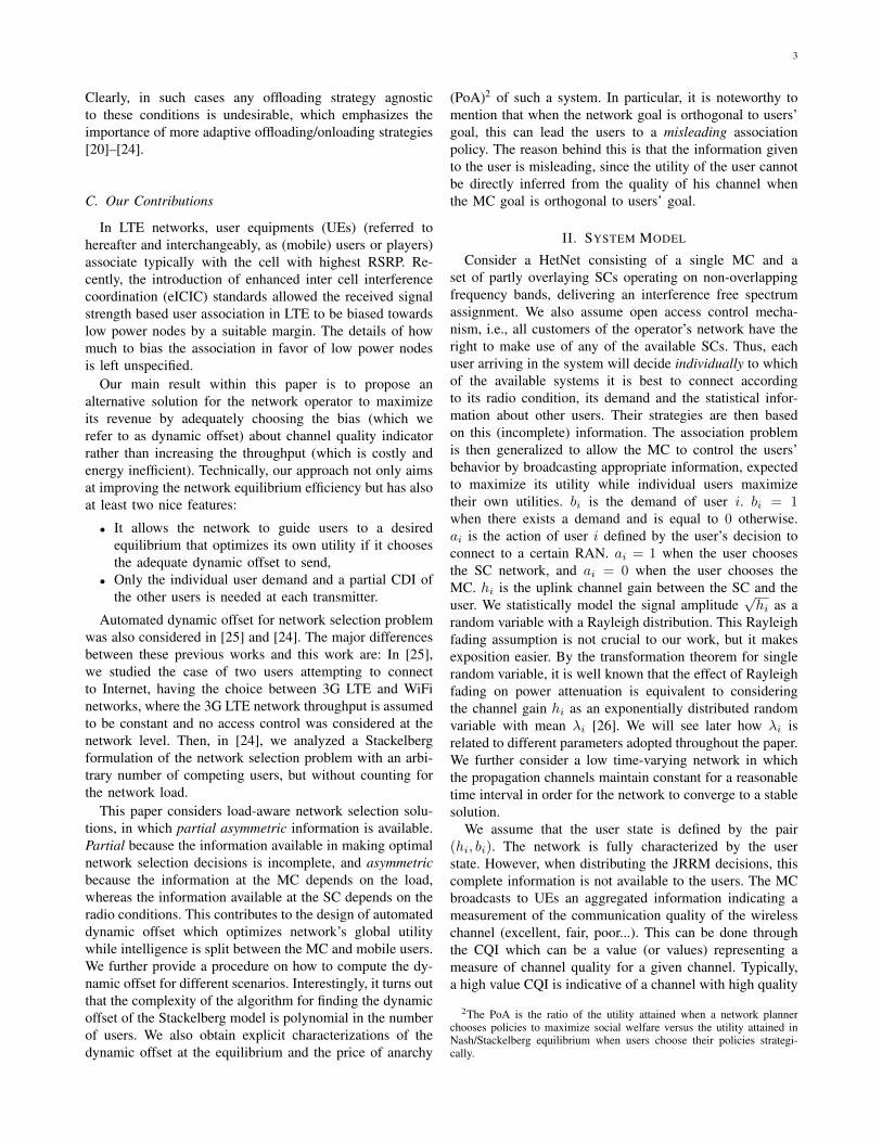
Fig. 1. Exemplary traffic steering to small cell in a heterogeneous network: Both real-time network load and radio conditions are important factors inmaking optimal network selection decisions.

schemes actually implemented by network operators arefully centralized: the operator tries to maximize his utility(revenue) by assigning the mobile users to different systems(for a survey refer to [5]). However, distributed joint radioresource management (JRRM) mechanisms are gaining inimportance: mobile users may be allowed to make au-tonomous decisions in a distributed way. In the same trend,[6] proposed a distributed algorithm which jointly determinethe amount of radio resources that MCs should offer toSCs, and the association rules that decide which mobileusers should associate with SCs. In [7], a network interfaceselection algorithm which maps user traffic across WiFi andLTE is implemented to optimize user QoE through adaptivetraffic offloading. Evaluations on a real LTE-WiFi testbedusing YouTube traffic reveals that video stalls are reducedby 3�4 times compared to naive solutions. In [8], a networkselection strategy considering small cell backhaul capacityis proposed and evaluated in terms of connection throughputand fairness. This has lead to game theoretic approaches tothe network selection problems in HetNets, as can be foundin [9]–[11]. [12] formulates the problem of user associationin the downlink of small cell networks as a many-to-onematching game, in which base stations are assumed to beaware of each user’s overall preferences.

Instead of taking part within the debate among thesupporters of each (centralized or distributed) solution, wepropose in this paper a Stackelberg formulation of thenetwork selection problem, where the operator optimizesits global utility by sending appropriate information, whilemobile users compete to maximize their throughput bypicking the best locally serving RAN. By Stackelberg wemean distributed decision making assisted by the network,where the wireless users aim at maximizing their ownutility, guided by aggregated information broadcasted by thenetwork about the channel distribution information (CDI)of each user. We derive the policy that corresponds tothe Stackelberg equilibrium and compare it to the fullycentralized (optimal), the full channel state information(CSI) and the non-cooperative (autonomous) models.

B. Partial InformationIn order to provide optimal use of RAN resources and

best end user experience, 3GPP is also working on theintegration of SC to include radio access technology (RAT)selection, addressed through per user and real time based de-cisions (e.g., network load and users’ radio conditions). Forexample, in Fig. 1, when the cellular network is somewhatcongested, the operator who controls both the MC and theSC networks may want to steer mobile users that experiencebad radio conditions on the cellular network (e.g., poorReceived Signal Reference Power (RSRP)1 for LTE) fromthe MC to the SC (assuming SCs are available). Mostexisting work so far have assumed that each BS or mobileuser has all others’ dynamics information whenever makingits resource allocation decisions [13]–[16]. Nevertheless,this might not be realistic in HetNets due to the limitedcapacity of the backhaul links and varied ownership ofnetwork devices [17], [18]. Moreover, obtaining/estimatingall the channel gains on each of the resource blocks is highlyimpractical, since it leads to an enormous amount of controloverheads. In order to find a desired trade-off betweenthe global network performance reached at the equilibriumand the amount of signaling needed to make it work, weinvestigate a strategy based on an automated dynamic offsetselection where only a partial CDI is assumed to be knownat the transmitter. We define the offset as the channelquality indicator (CQI) which represents a measure of thechannel quality. This is a challenging network selectionproblem, whose solution is critical for many applicationsand use-cases in future wireless systems. Indeed, it hasbeen shown that aggressively offloading mobile users fromMC to SCs can lead to degradation of user-specific aswell as network wide performance. On the other hand, aconservative approach may result in load disparity, whichnot only leads to underutilization of resources but alsodegrades the performance of multimedia applications [19].

1RSRP is a measure of the received signal strength of a cell at a mobileuser and it is measured based on the strength of certain reference signalsthat cells broadcast.

3

Clearly, in such cases any offloading strategy agnosticto these conditions is undesirable, which emphasizes theimportance of more adaptive offloading/onloading strategies[20]–[24].

C. Our Contributions

In LTE networks, user equipments (UEs) (referred tohereafter and interchangeably, as (mobile) users or players)associate typically with the cell with highest RSRP. Re-cently, the introduction of enhanced inter cell interferencecoordination (eICIC) standards allowed the received signalstrength based user association in LTE to be biased towardslow power nodes by a suitable margin. The details of howmuch to bias the association in favor of low power nodesis left unspecified.

Our main result within this paper is to propose analternative solution for the network operator to maximizeits revenue by adequately choosing the bias (which werefer to as dynamic offset) about channel quality indicatorrather than increasing the throughput (which is costly andenergy inefficient). Technically, our approach not only aimsat improving the network equilibrium efficiency but has alsoat least two nice features:

• It allows the network to guide users to a desiredequilibrium that optimizes its own utility if it choosesthe adequate dynamic offset to send,

• Only the individual user demand and a partial CDI ofthe other users is needed at each transmitter.

Automated dynamic offset for network selection problemwas also considered in [25] and [24]. The major differencesbetween these previous works and this work are: In [25],we studied the case of two users attempting to connectto Internet, having the choice between 3G LTE and WiFinetworks, where the 3G LTE network throughput is assumedto be constant and no access control was considered at thenetwork level. Then, in [24], we analyzed a Stackelbergformulation of the network selection problem with an arbi-trary number of competing users, but without counting forthe network load.

This paper considers load-aware network selection solu-tions, in which partial asymmetric information is available.Partial because the information available in making optimalnetwork selection decisions is incomplete, and asymmetricbecause the information at the MC depends on the load,whereas the information available at the SC depends on theradio conditions. This contributes to the design of automateddynamic offset which optimizes network’s global utilitywhile intelligence is split between the MC and mobile users.We further provide a procedure on how to compute the dy-namic offset for different scenarios. Interestingly, it turns outthat the complexity of the algorithm for finding the dynamicoffset of the Stackelberg model is polynomial in the numberof users. We also obtain explicit characterizations of thedynamic offset at the equilibrium and the price of anarchy

(PoA)2 of such a system. In particular, it is noteworthy tomention that when the network goal is orthogonal to users’goal, this can lead the users to a misleading associationpolicy. The reason behind this is that the information givento the user is misleading, since the utility of the user cannotbe directly inferred from the quality of his channel whenthe MC goal is orthogonal to users’ goal.

II. SYSTEM MODEL

Consider a HetNet consisting of a single MC and aset of partly overlaying SCs operating on non-overlappingfrequency bands, delivering an interference free spectrumassignment. We also assume open access control mecha-nism, i.e., all customers of the operator’s network have theright to make use of any of the available SCs. Thus, eachuser arriving in the system will decide individually to whichof the available systems it is best to connect accordingto its radio condition, its demand and the statistical infor-mation about other users. Their strategies are then basedon this (incomplete) information. The association problemis then generalized to allow the MC to control the users’behavior by broadcasting appropriate information, expectedto maximize its utility while individual users maximizetheir own utilities. b

i

is the demand of user i. b

i

= 1

when there exists a demand and is equal to 0 otherwise.a

i

is the action of user i defined by the user’s decision toconnect to a certain RAN. a

i

= 1 when the user choosesthe SC network, and a

i

= 0 when the user chooses theMC. h

i

is the uplink channel gain between the SC and theuser. We statistically model the signal amplitude

ph

i

as arandom variable with a Rayleigh distribution. This Rayleighfading assumption is not crucial to our work, but it makesexposition easier. By the transformation theorem for singlerandom variable, it is well known that the effect of Rayleighfading on power attenuation is equivalent to consideringthe channel gain h

i

as an exponentially distributed randomvariable with mean �

i

[26]. We will see later how �

i

isrelated to different parameters adopted throughout the paper.We further consider a low time-varying network in whichthe propagation channels maintain constant for a reasonabletime interval in order for the network to converge to a stablesolution.

We assume that the user state is defined by the pair(h

i

, b

i

). The network is fully characterized by the userstate. However, when distributing the JRRM decisions, thiscomplete information is not available to the users. The MCbroadcasts to UEs an aggregated information indicating ameasurement of the communication quality of the wirelesschannel (excellent, fair, poor...). This can be done throughthe CQI which can be a value (or values) representing ameasure of channel quality for a given channel. Typically,a high value CQI is indicative of a channel with high quality

2The PoA is the ratio of the utility attained when a network plannerchooses policies to maximize social welfare versus the utility attained inNash/Stackelberg equilibrium when users choose their policies strategi-cally.

4

Parameter Description�2 the noise variance,bi

the demand of user i. bi

= 1 when there exists ademand, and 0 otherwise,

�i

the probability that bi

= 1,hi

the uplink channel power gain between the SC and theuser with mean �

i

,

i

the dynamic offset parameter (or CQI threshold) of useri set by the MC,

si

the channel state of user i. si

= 1 if the channel isgood, and s

i

= 0 otherwise,↵i

the probability to have hi

> i

, which corresponds tothe probability to have s

i

= 1,ai

the action of user i. ai

= 1 when the user chooses theSC, and 0 when the user chooses MC,

P the policy profile matrix,D the MC peak rate,G the opportunistic scheduler gain,

vmin

the lower (minimal) throughput of the streaming service,vmax

the upper (best) throughput of the streaming service.

TABLE IDESCRIPTION OF THE VARIOUS PARAMETERS.

and vice versa. More formally, assume that the knowledgeof each user about his own state is limited to the pair(s

i

, b

i

), where s

i

= 1I{hi

> i

}, with i

– a fixed threshold,and 1I

C

is the indicator function equal to 1 if conditionC is satisfied and to 0 otherwise. We will call

i

the CQIthreshold of user i, referred to hereafter and interchangeablyas dynamic offset. Thus, a user only knows whether hewants to transmit and whether the channel is in a goodcondition (s

i

= 1) or in a bad condition (si

= 0) given theCQI threshold. In addition, any player has the informationabout the probability distribution of his own state (s

i

, b

i

)

and that of his opponent (sj

, b

j

). These are given by ↵

i

– theprobability to have h

i

>

i

, and �

i

– the probability that thedemand b

i

= 1. Let us denote by P = [P1, . . . ,Pn]T the

(n⇥ 2) policy profile matrix, whose element Pi representsthe action vector taken by the mobile user i in low and highchannel states for i = {1, . . . , n}. The various parametersused throughout the paper are listed in Table I.

In the next sections, we provide a thorough analysis ofthe existence and characterization of the Bayes equilibriafor both non-cooperative and Stackelberg scenarios. We firstfocus on the two-user case in order to gain insights into howto design decision problem in mobile wireless environments.Then, we generalize our approach to the multi-user case.

The first step before analyzing the Stackelberg Bayesiandecision scheme is to define the utilities of the users. Theseare often related to throughput, whose variations are mainlydue to network load and radio conditions.A. The Macro Cell Throughput

When performing network selection decisions, the mo-bile can benefit from knowledge about real time networkconditions and quality parameters. In addition, the cellularnetwork congestion condition need to be considered. Thisallows the UE to perform access decisions not only based onthe viability of the SC network, but also on the conditionson the MC access to determine the need to move traffic to

SC and when such traffic can indeed be moved back to theMC network.

Motivated by the fact that the exponential growth inmobile traffic is primarily driven by streaming service, weconsider a real-time transport protocol (RTP) streamingservice which takes into account both the cellular networkcongestion and the mobile user’s radio conditions. The UE’sutility is expressed by the quality of his streaming flow,which is in turn closely related to his throughput. Indeed,a streaming call with a higher throughput will enable theUE to stream the video at a higher bit rate and thereforeoffering a better video quality. The goal of a streaminguser is thus to achieve the best throughput of between anupper (best) v

max

and a lower (minimal) vmin

bounds (withv

max

> v

min

). This throughput depends not only on thepeak throughput, but also on the evolution of the number ofcalls in the system where the user decides to connect. Notethat a user that cannot be offered this minimal throughputin neither of the available systems is blocked in order topreserve the overall network performance. However, onceconnected, we suppose that a call will not be dropped evenif its radio conditions degrade because of mobility.

Assuming fair scheduling among different users, thethroughput of a user connected to the MC when there aren0 users admitted to MC is given by:

v = min

D ·GP

n0

i=1(1� a

i

)b

i

, v

max

�(1)

where G is the opportunistic scheduler gain and D is theMC peak rate (i.e., the throughput a user would obtainif he were alone in the cell). Here, we assume that theMC has sufficient resources to guarantee to every user thethroughput he requires depending on his demand and thesystem load. Note that the admission control will ensurethat v � v

min

by blocking new arrivals. Without loss ofgenerality, we may assume also that DG � v

max

.

B. The Small Cell ThroughputThe measurement of average throughput of a node in a SC

network is done by the time it takes to transfer the files be-tween the SC and the mobile users. The throughput dependson the bit rate at which the wireless mobile communicatesto its SC, which greatly depends on the attenuation levelat the receiver side due to his geographical position. Thiscan vary greatly depending on the link conditions. The SCthroughput can thus be expressed by

log2

✓1 +

p h

i

a

i

b

i

�

2

◆(2)

where �

2 is the noise variance and p the user’s transmitpower. Notice that, in (2), we consider that there is noresource partitioning (and thus no interference) between theMC and the SC as they both operate on non-overlappingfrequency bands.

The utility we have considered in (2) is better suitedfor lightly loaded SCs or for situations where each user

5

is only given a tiny fraction of the SC resources regardlessof the load assuming that this fraction is small enough thatthe SC can support all users [23]. Of course, this comesat the expense of decreasing the spectral efficiency of thenetwork. However, we shall notice that there exists a plentyof scenarios where such a situation is met, notably situationswith priority among users. For example, when resourceallocation rules correspond to those of primary users incognitive radio or spectrum pooling networks, in whicheach user enjoys only a limited access to the spectrum. Therationale behind this stems from the fact that primary usersmaximizing their own spectral efficiency independently ofthe others can result in suboptimal usage of the spectrum[27].

Remark 1. The BS depends crucially on truthful reportingof their channel states by the UEs. For example, in thefrequency-division duplex (FDD) system, the BS has nodirect information on the channel gains, but transmitsdownlink pilots, and relies on the UEs’ reported valuesof gains on these pilots for scheduling. A cooperative UEwill truthfully report this information to the BS. A non-cooperative UE will however send a signal that is likelyto induce the scheduler to behave in a manner beneficialto the UE. In our case and since we consider the uplinkscenario, users do not distribute anything except theirnetwork preference list (see Fig. 2), which are obviouslydistributed honestly.

Given �

i

and i

, we can compute that the distributionof h

i

is Exp(�i

) with

↵

i

= Pr{hi

>

i

} = exp(��

i

i

) (3)

Knowing the information that a player has, there are fourpossible policies of a player i with b

i

= 1 (we do notconsider state b

i

= 0, when there is no transmission of anytype):

h

i

<

i

S S M M

h

i

>

i

S M S M

where indices M and S stand for the MC (i.e., ai

= 0) andthe SC (i.e., a

i

= 1) respectively. Notice that the top rowcorresponds to s

i

= 0 while the bottom row correspondsto s

i

= 1. In the sequel, we will refer to these fourpolicies shortly as SS, SM , MS and MM policies. Letus not consider the policy SM , which is irrational, as thethroughput of a player using the SC when h

i

>

i

iscertainly higher than that when h

i

<

i

. We then havea game with partial CDI with two states and 3 actions foreach player in every state.

III. THE TWO-USER CASE

For the ease of comprehension, we will begin by consid-ering the two-user case and then generalize the results tothe multi-user case later in Section IV.

A. UtilitiesUser i’s utility in state s = 0, 1 is then given by

u

i

(s,P) =

⇢v

i

Pj; if user i chooses M at state s,

C

i

(s); if user i chooses S at state s.(4)

The functions C

i

(s), describing the utility of player i

using the SC network at state s, are defined as follows

C

i

(1) = [c

i

(h

i

)|hi

>

i

] =

1

↵

i

Z 1

i

c

i

(h

i

)�

i

e

��

i

h

i

dh

i

,

C

i

(0) = [c

i

(h

i

)|hi

<

i

] =

1

1� ↵

i

Z i

0c

i

(h

i

)�

i

e

��

i

h

i

dh

i

,

c

i

(h

i

) above is the utility of player i using S whenchannel gain is h

i

and is defined as follows:

c

i

(h

i

) = log2

⇣1 +

ph

i

�

2

⌘(5)

On the other hand, the utilities v

i

k

of player i using theMC in (4), when player j applies policy k, are defined asfollows

v

i

SS

= v

max

(6)

Next,

v

i

MS

= [↵

j

+ (1� �

j

)(1� ↵

j

)]v

max

+ �

j

(1� ↵

j

)min{DG

2

, v

max

}1I{DG

2 �v

min

}

+ �

j

(1� ↵

j

)

v

max

2

1I{DG

2 <v

min

} (7)

Finally,

v

i

MM

= (1� �

j

)v

max

+ �

j

min{DG

2

, v

max

}1I{DG

2 �v

min

}

+ �

j

v

max

2

1I{DG

2 <v

min

} (8)

The utilities for the last two cases reflect the fact thatsome arrivals may be blocked by the admission controlwhen there is not enough resource for all the players - inthat case we assume that some k players (where k is suchthat DG

k

� v

min

) willing to connect to the MC networkare chosen at random (with equal probabilities)3 and theyreceive the service4. Note that the utilities defined abovesatisfy the following sets of inequalities:

C

i

(1) > C

i

(0), (9)

v

max

= v

i

SS

� v

i

MS

� v

i

MM

> (1� �

j

)v

max

. (10)

3More precisely, the quantities appearing in (7) and (8) can be interpretedas follows: The term multiplied by v

max

is the probability that i is theonly player using MC, the term appearing before min{DG

2 , vmax

} andv

max

2 is the probability that there are two players requesting connectionto MC. Then if DG

2 < vmin

, one player is chosen at random, so hisutility is v

max

with probability 12 and 0 with probability 1

2 . Otherwiseboth players are admitted and their utility is min{DG

2 , vmax

}.4In reality the ones chosen at random in our model would be those

whose request was considered first.

6

B. The non-cooperative equilibrium

Game theory has accentuated the importance of random-ized games or mixed games. However, such a game does notfind any significant role in most communication modemsor source coding codecs since equilibria where each userrandomly picks a decision at each time epoch cannot beused effectively there, as they amount to perpetual handoverbetween networks.

Definition 1 (Bayes-Nash equilibrium). A strategy profilePi

BNE , 8i = 1, 2 corresponds to a Bayes-Nash equilibrium(BNE) if, for all users, any unilateral switching to a differentstrategy cannot improve user’s payoff at any state. Mathe-matically, this can be expressed by the following inequality,given the CDI about the other user 8 Qi 6= Pi

BNE and fors

i

= {0, 1}u

i

(s

i

, (PiBNE

,P�iBNE

)) � u

i

(s

i

, (Qi,P�iBNE

));

where the "�i" subscript on vector P stands for "exceptuser i".

Proposition 1. The game considered in the paper alwayshas a pure-strategy Bayes-Nash equilibrium. Moreover(a) (SS, SS) is an equilibrium iff Ci

(0) � v

i

SS

for i = 1, 2.(b) (SS,MS) is an equilibrium iff C

1(0) � v

1MS

andC

2(1) � v

2SS

� C

2(0).

(c) (SS,MM) is an equilibrium iff C

1(0) � v

1MM

andC

2(1) v

2SS

.(d) (MS,SS) is an equilibrium iff C1

(1) � v

1SS

� C

1(0)

and C

2(0) � v

2MS

.(e) (MS,MS) is an equilibrium iff Ci

(1) � v

i

MS

� C

i

(0)

for i = 1, 2.(f) (MS,MM) is an equilibrium iff C

1(1) � v

1MM

�C

1(0) and C

2(1) v

2MS

.(g) (MM,SS) is an equilibrium iff C

1(1) v

1SS

andC

2(0) � v

2MM

.(h) (MM,MS) is an equilibrium iff C

1(1) v

1MS

andC

2(1) � v

2MM

� C

2(0).

(i) (MM,MM) is an equilibrium iff C

i

(1) v

i

MM

fori = 1, 2.

Proof: The statements (a)–(i) are direct consequencesof the definition of Bayes-Nash equilibrium and the formof payoff matrices. Next, using inequalities (9,10), it isstraightforward to show that we always have at least oneof the conditions (a)–(i) satisfied.

The next proposition gives us some information on howthe Nash-Bayes equilibria depend on the chosen values ofthe CQI thresholds

i

.

Proposition 2. For any player i, if i

is the small enough,player i does not use policy SS in equilibrium. If it is largeenough, player i does not use policy MM in equilibrium.Next define for i = 1, 2

C

i

(1) =

Z 1

0c

i

(h

i

)�

i

e

��

i

h

i

dh

i

(11)

If C

i

(1) 6= v

max

for i = 1, 2, then for all the values ofthe parameters of the model one of the three possibilities istrue:(a) For 1 and 2 small enough, both players use policy

MM in equilibrium,(b) For 1 and 2 large enough, both players use policy

SS in equilibrium,(c) For

i

small enough, i uses policy MM in equilib-rium, while for

j

large enough j uses policy SS inequilibrium.

Proof: Note that5:1) when

i

! 0, Ci

(0)(

i

) ! 0, Ci

(1)(

i

) ! C

i

(1)

and v

j

MS

(

j

) ! v

j

SS

for i = 1, 2;2) when

i

! 1, C

i

(0)(

i

) ! C

i

(1), C

i

(1)(

i

) !+1 and v

j

MS

(

j

) ! v

j

MM

.Thus for

i

small enough, Ci

(0)(

i

) < v

i

MM

, which byProposition 1 implies that player i does not use policy SS inequilibrium. Analogously for

i

big enough, Ci

(1)(

i

) >

v

i

SS

, and so player i does not use MM in equilibrium then.Let us assume now that both 1 and 2 are either

very small or very large and that in both situations theequilibrium is of type (MS,MS). By Proposition 1, thisimplies that

C

i

(1)(

i

) � v

i

MS

(

j

) � C

i

(0)(

i

)

for i = 1, 2 in both situations ( i

s small or large). Nowtaking into account properties 1) and 2) described above,we can pass to the limit as

i

! 0, i = 1, 2, getting:

C

1(1) � v

i

SS

� 0 for i = 1, 2. (12)

Analogously, passing to the limit as i

! 1, i = 1, 2, weobtain

1 � v

i

MM

� C

1(1) for i = 1, 2. (13)

But (12) together with (13) contradict (10) as long asv

max

6= C

i

(1).We prove similarly that neither of the situations enumer-

ated below is possible: one of the profiles (MS,MM) or(MM,MS) is an equilibrium for

i

s approaching 0 and(MS,MS) is an equilibrium for

i

s approaching infinity,or (MS,MS) is an equilibrium for

i

! 0 and (MS,SS)

or (SS,MS) is an equilibrium for i

! 1.The result of this proposition can be interpreted in the

following manner: for higher values of the CQI thresholds

i

the players prefer to use the SC rather than the MCand conversely, for low

i

s they prefer to use the MC.Interestingly, Proposition 2 also suggests that, rather thanincreasing the offered throughput v, the operator couldcontrol the equilibrium of its wireless users to maximize itsown revenue by broadcasting appropriate CQI thresholds.This can lead the network to minimize its overall costand users to a misleading association problem. Next, we

5In what is written below we use the convention that Ci(s)( i

) meansthe value of Ci(s) when i’s CQI threshold is

i

, similarly viMS

( j

) isthe value of vi

MS

when his opponent’s threshold is j

. Analogously forother functions.

7

extend the analysis of the above mentioned problem usinghierarchical approach.

C. The hierarchical equilibrium

In this section, we propose a methodology that transformsthe above non-cooperative game into a Stackelberg game.Concretely, the MC network may guide users to an equilib-rium that optimizes its own utility U

MC

if it chooses theadequate information to send. We first study the policy thatmaximizes the utility of the network, which is defined asthe expected throughput of the MC network (we need todefine it using two steps):

UMC

(q1, q2) = [q1(1� q2) + q2(1� q1)]vmax

+

q1q2[DG1I{vmin

DG

2 v

max

}+

2v

max

1I{vmax

<

DG

2 } + v

max

1I{DG

2 <v

min

}],

where q1 and q2 are the probabilities that player 1, respec-tively player 2, uses the MC. Consequently

U

MC

(P, 1, 2) = UMC

(q(P1, 1), q(P2, 2))

with q(Pi

,

i

) = �

i

⇥1I{P

i

=MM} + (1� e

��

i

i

)1I{Pi

=MS}⇤.

Nevertheless, as it is not realistic to consider that theusers will seek the global optimum, we show how tofind the policy that corresponds to the Bayes-Stackelbergequilibrium where the MC tries to maximize U

MC

just bychoosing the CQI thresholds, knowing that users will try tomaximize their individual utility.

Definition 2 (Bayes-Stackelberg equilibrium). By de-noting ( 1

BSE

, 2BSE

) the strategy profile of the MCat a Bayes-Stackelberg equilibrium (BSE), this definitiontranslates mathematically as

( 1BSE

, 2BSE

) 2 arg max

1, 2

U

MC

(PBNE

( 1, 2), 1, 2),

(14)where PBNE

( 1, 2) is any Bayes-Nash equilibrium in thegame of the previous section with CQI thresholds equal to 1, 2.

We next exemplify our general analysis by investigatingthe possibility of considering three scenarios for the choiceof 1 and 2:

1) Centralized model – the MC chooses both i

s andthe policies for the players, aiming to maximize U

MC

.Formally, the centralized strategy is the one satisfying

( 1C

, 2C

,PC

) 2 arg max

1, 2,PU

MC

(P, 1, 2),

2) Stackelberg model – there are two stages: at the firstone the MC chooses both

i

s given the informationabout the distributions of (h

i

, b

i

) aiming to maximizethe throughput of the MC network at the second stage,when players play the game from the last section.The proposed approach can be seen as intermediatescheme between the centralized model and the fullynon-cooperative model,

3) Fully non-cooperative model – the game has twostages: at the first one, players choose their

i

s giventhe information they have about the distributions of(h

i

, b

i

) aiming to maximize their expected throughputat the second stage; at the second stage they choosea policy depending on actual (s

i

, b

i

) as in the modelof the last section. Formally, a fully non-cooperativestrategy is any one satisfying

NC

i

2 argmax

i

E[ui

(s

i

,PBNE

(

i

,

NC

j

))]; for i = 1, 2

with PBNE

(

i

,

NC

j

) being any Bayes-Nash equilib-rium in the game of the previous section.

Remark 2. The name fully non-cooperative suggests adifferent model, without two stages, where the decisionboth about the CQI thresholds and about players’ policiesis made by the users at the same time. As it will beshown in Proposition 4, the two models are equivalent.The two-step procedure that we propose only makes a cleardistinction between stage one when no communication isneeded, because all the data necessary to compute the

i

isavailable to all the players and the MC, and stage two whenthe information about channel quality has to be reported tothe players to assign them to MC or to SC. Thus, as in all theother scenarios that we provide, the amount of informationthat has to be transmitted during the game is very limited.

Below, we analyze the behavior of the MC and the playersat the equilibria of each of these models.

Proposition 3.1) In the centralized model, the MC chooses any 1 and 2, and MM policy for both users.

2) In the Stackelberg model, the MC does the followingsteps:a) Computes C

i

(1) for i = 1, 2. If C1(1) v

1MM

and C

2(1) v

2MM

, then it chooses any 1 <

⇤⇤1 and 2 <

⇤⇤2 with

⇤⇤i

satisfyingC

1(1)(

⇤⇤1 ) = v

1MM

and C

2(1)(

⇤⇤2 ) = v

2MM

andthen users both play MM in the second stage.b) It finds6

1, 2 solving three maximizationproblems:b1: maximize U

MC

(�1(1 � e

��1 1),�2) subject

to v

1MS

( 2) � C

1(1), C

2(1)( 2) � v

2MM

�C

2(0)( 2);

b2: maximize UMC

(�1,�2(1 � e

��2 2))

subject to C

1(1)( 1) � v

1MM

� C

1(0)( 1),

v

2MS

( 1) � C

2(1);

b3: maximize UMC

(�1(1� e

��1 1),�2(1� e

��2 2))

subject to C

1(1)( 1) � v

1MS

( 2) � C

1(0)( 1),

C

2(1)( 2) � v

2MS

( 1) � C

2(0)( 2).

It chooses the biggest of the three value functionsV

b

(if some of these problems has no solutions weassume the value of its value function is 0) and 1, 2 solving this problem is what it plays at the first

6If some problem does not depend on i

, we take i

= 0.

8

stage of the game. At the second stage players choosepolicies (MS,MM), (MM,MS) and (MS,MS) ifthe solution of problem b1, b2 and b3 (respectively)was chosen by the MC.

3) In the fully non-cooperative model, the players inequilibrium choose 1 =

⇤1 and 2 =

⇤2 satisfying

c

1(

⇤1) = v

1MS

, c

2(

⇤2) = v

2MS

(15)

and then both use a MS policy.

For the clarity of the exposition, proofs are given in theAppendix. What we see in this proposition is that when theMC can decide on the behavior of the users, it forces themto use the MC. In other cases (when users can decide ontheir behavior, but are given only partial information), theusers’ interest is to choose the CQI thresholds somewhere inthe middle of the channel gain range. On the other hand, theMC has an incentive to choose CQI thresholds either verylow (first case in the Stackelberg scenario) or very high (thesecond case). Both these choices give little information forthe user about actual channel condition, which is what hewants to avoid. It is interesting and somewhat surprising thatthe optimal policy of the MC in the Stackelberg game can beboth giving high or low values of CQI thresholds. This canhowever be explained when we understand the meaning ofthese two situations – very low value of the threshold meansthat no information about the channel state is given. In thiscase, when both users connect to the MC, this correspondsto the choice of the MC. Now, if in the "no information"case players choose the SC network, then the MC tries todivide the range of h

i

into a small (in terms of probability)part when the players use the SC and, a large one when theyuse the MC. This is done by giving the highest possible CQIthreshold below which the players would have an incentiveto use rather the MC than the SC. This explains why theMC has an incentive to choose CQI thresholds very high inthis case.

In the next proposition, we show that the strategieschosen by the players in the fully non-cooperative scenarioof Proposition 3 are also equilibria in two other non-cooperative models, differing from the one considered aboveby the time the decisions are made by the players or theamount of information available to them.

Proposition 4. Consider two alternative non-cooperativemodels:(M1) The game has one stage, at which the players choose

both CQI thresholds and policies they apply, aimingto maximize their own throughput. They base theirchoices on the information about distributions of(h

i

, b

i

).(M2) The game has one stage, at which the players choose

whether they want to connect to MC or SC, aimingto maximize their own throughput. Each player knowsthe distribution of (h

j

, b

j

) of the opponent and exactvalues of his own h

i

and b

i

.

If ⇤1 and ⇤

2 are CQI thresholds chosen in part 3) ofProposition 3, then ⇤

1- and ⇤2-threshold policies (that

is - MS policies with

⇤i

CQI thresholds) are also inequilibrium in models (M1) and (M2).

The final result of this section is given without proof,which is straightforward. In that result, we give the methodto compute the PoA for our model. Remind that the PoAmeasures how good the system performance is when usersplay selfishly and reach the NE instead of playing to achievethe social optimum obtained in the centralized model withutility U

MC

(�1,�2). Thus the PoA when players use strat-egy profile P is

PoA =

UMC

(�1,�2)

UMC

(q(P1, 1), q(P2, 2)).

Thus, Proposition 3 implies that

Corollary 1. The PoA in the Stackelberg model equals 1

whenever C

i

(1) v

i

MM

for i = 1, 2. When for some i,C

i

MM

(1) > v, then the PoA is equal to

UMC

(�1,�2)

V

b

,

where V

b

is the value of the objective function computed inProposition 3.

In fully non-cooperative model,

PoA =

UMC

(�1,�2)

UMC

(�1(1� e

��1 ⇤1),�2(1� e

��2 ⇤2))

,

where ⇤1 and ⇤

2 satisfy (15).

The above corollary is just a rewriting of the Proposition3 using different language.

IV. THE MULTI-USER CASE

Now, let us consider the case where instead of two wehave n users choosing to connect either to the SC or tothe MC network. Again we assume that the informationabout the channel quality that user i possesses is limitedto that about the distributions of states (s

j

, b

i

) of each ofthe players (including i), that is about ↵

j

(or �

j

) and �

j

and to exact information about his own current state (s

i

, b

i

)

(but not about exact value of h

i

). We make two additionalassumptions about the model considered in this section. Thefirst one is that the model is symmetric, that is all the values�

i

,�

i

and i

defining it, are the same for each of the players(and equal to �,� and respectively). The second one isthat v

max

� 2v

min

. Both of them aim at simplifying thenotation used in our considerations. On the other hand, webelieve that some counterparts of all our results are true alsowithout these assumptions, so they can be made withoutserious limitation of generality.

A. UtilitiesAgain we assume that each of the players uses one of the

three policies SS,MS,MM , where first letter stands for aplayer’s action when his channel is bad, and the second

9

one when his channel is good. As it is troublesome to writedown the policies for each of n players, we will make useof the fact that the game is symmetric, writing instead ofthe policy profile a policy statistics K = [k

MM

, k

MS

] withk

MM

denoting the number of players applying policy MM

and k

MS

– of players applying MS. Of course the numberof those using policy SS is n�k

MM

�k

MS

, so we will omitit. Given K, we can define user i’s utility in state s = 0, 1

as7

u

i

(s,K) =

⇢vK�i

; if user i chooses M at state s,

C(s); if user i chooses S at state s

(16)where C(s) is defined as C

i

(s) for two-user case, with thesuperscript omitted because the model is symmetric, whilethe values vK�i

, describing the utility of player i using theMC when his opponents use policies described by K, aresimilarly as for the two-user case8:

v[k,l] =

Pk

r=0

Pl

q=0

Pq

w=0 �r+q

(1� �)

k+l�r�q

✓k

r

◆✓l

q

◆✓q

w

◆

·e��(q�w) (1� e

�� )

w

min{k⇤,r+w+1}

r+w+1

·min{ DG

min{k⇤,r+w+1} , vmax

}(17)

where k

⇤= max{k :

DG

k

� v

min

} is the biggest numberof users that can be admitted to MC without decreasingtheir throughputs below v

min

(remember that, as in the two-player case, the utility defined above is the expected value ofuser’s throughput, already taking into account the admissioncontrol).B. The equilibria

Below, we give a generalization of Proposition 1 for then-user case.

Proposition 5. The symmetric n-user game considered inthe paper always has a pure-strategy Bayes-Nash equilib-rium of one of seven types:(a) When v[k�1,l] � C(1) � v[k,l�1] � C(0) � v[k,l],

then any profile where k players use policy MM , l

players use policy MS, and all the others play SS isan equilibrium.

(b) When v[k�1,0] � C(1) � C(0) � v[k,0] then any profilewhere k players apply policy MM and the remainingn� k players use policy SS is an equilibrium.

(c) When v[k�1,n�k] � C(1) � v[k,n�k�1] � C(0) thenany profile where k players apply policy MM andthe remaining n � k players use policy MS is anequilibrium.

(d) When v[n�1,0] � C(1) then the profile where all theplayers use policy MM is an equilibrium.

(e) When C(1) � v[0,k�1] � C(0) � v[0,k], then any profilewhere k players use policy MS and all the others playSS is an equilibrium.

7Notation K�i used below denotes policy statistics defined as in thetwo-user case but without policy of user i.

8Of S as this is a generalization of the formulas for vik

given in SectionIII and it applies for any n � 2, in particular vi

MM

⌘ v[1,0], viSC

⌘v[0,1] and vi

SS

⌘ v[0,0] when n = 2 and players are symmetric.

(f) When C(1) � v[0,n�1] � C(0) then the profile whereall the players use policy MS is an equilibrium.

(g) When C(0) � v[0,0] then the profile where all theplayers use policy SS is an equilibrium.

We give a corollary to this proposition. It gives a kindof consistency property for equilibria in games for differentvalues of n.

Corollary 2.(a) Suppose that a profile where at least one player uses

policy SS and the number of players using policiesMM and MS is k, is an equilibrium in n-user sym-metric game. Then it is also an equilibrium in any m-user game defined with the same parameters �,� and and m � k.

(b) Moreover for any fixed parameters �,� and thereexists an m such that for any n > m at least n �m players use policy SS in any equilibrium in n-usergame.

Proof: Note that v[k,l] does not depend on the numberof players in the game n, only on the number of those whouse one of the policies MS or MM . Just this implies part(a). Part (b) is due to the fact that v[k,l] ! 0 as eitherk ! 1 or l ! 1.

The next proposition generalizes the results for hierarchi-cal model included in Proposition 3 for n-user symmetricgames. We consider all the above scenarios, yet in scenario3) we only show that the equilibrium is symmetric, butassume that players may act asymmetrically in general. Todo so we look for symmetric equilibria in the model (whichexist, but we believe are not the only ones possible there,even though the model itself is symmetric). The rationalebehind this simplification is twofold: firstly – consideringasymmetric equilibria would cause various problems withnotation; secondly and most important – we believe thatasymmetric equilibria, where users may have different func-tional form of their strategies, are harder to justify, as theywould require prior coordination among the devices to agreeon which equilibrium is played.

The MC utility, defined as before, as the expectedthroughput of the MC network, can be now written as:

U

MC

([k, l], ) =

kX

r=0

lX

q=0

qX

w=0

�

r+q

(1� �)

k+l�r�q

·✓k

r

◆✓l

q

◆✓q

w

◆e

��(q�w) (1� e

�� )

w

·min{DG, v

max

(w + r)}.(18)

Proposition 6.1) In the centralized model, the MC chooses any value of and MM policy for all the users.

2) In the Stackelberg model, the MC computes C(1) (see(11)) and finds k

⇤⇤ such that

v[k⇤⇤�1,0] > C(1) � v[k⇤⇤,0]. (19)

10

If such a k

⇤⇤ does not exist, it sets k

⇤⇤= 0. Next:

(a) If n k

⇤⇤ then at the equilibrium the MC choosesany such that v[n�1,0] � C(1)( ), and all theplayers use policy MM .

(b) If n > k

⇤⇤ then:b1) for any k such that k

⇤⇤ k n and any0 l k

⇤⇤ the MC does the following steps: itfinds such that

C(1)( ) = v[l�1,k�l]( ). (20)

If such a does not exist or C(0)( ) <

v[l,k�l]( ), it puts P (k, l) = 0. Otherwise it finds such that

C(0)( ) = v[l,k�l�1]( ) (21)

If such a does not exist, it puts = 1.Finally, if P (k, l) has not been defined yet, it takes (k, l) = min{ , } and computes

P (k, l) = U

MC

([l, k � l], (k, l)).

b2) it chooses k

max

and l

max

with the biggestvalue of P (k, l) (which equals the MC utility atequilibrium). The choice of (k

max

, l

max

) at thefirst stage and any profile of policies where l

max

players use policy MM and k

max

�l

max

play MS

will then be an equilibrium.3) In the fully non-cooperative model, the players choose

⇤ satisfying

c(

⇤) = v[0,n�1](

⇤), (22)

and then all use MS policy at the second stage of thegame.

In order to compare the network utility under differentmodes, we give two corollaries to this proposition.

Corollary 3. The PoA in the n-user hierarchical model canbe computed as

PoA =

U

MC

([n, 0], )

U

MC

(K, )

(where U

MC

([n, 0], ) is the maximum value of the MC’sutility obtained in scenario 1) of Proposition 6), which isindependent of . Moreover:

1) In the Stackelberg model it is either equal to 1 whenk k

⇤⇤, or satisfies

PoA = min

k

⇤⇤kn,0lk

U

MC

([n, 0], )

P (k, l)

with k

⇤⇤ and P (k, l) defined as in Proposition 6.2) In the fully non-cooperative model it can be computed

as:PoA =

U

MC

([n, 0], )

U

MC

([0, n],

⇤)

with ⇤ defined as in Proposition 6.

The corollary is again just a rewriting of the results fromProposition 6 with the stress made on network utilities ratherthan strategies of the players. It shows that exactly the sameprocedure, used to find the equilibrium policies, can beapplied to evaluate the performance of the network.

V. THE NON-COOPERATIVE FULL CSI MODEL

In this section, we consider a model where every playerhas full information about the quality of channels andamount of data to be transmitted by each of the players. Itmeans that the players use exact information about their ownCSI in their decisions, not only the indication whether it isgood or bad, and also that they use exact information aboutthat of the others, not limited to their distributions. Noticethat the non-cooperative full CSI scheme is not realistic asit is not feasible to consider that the network operator willdivulge users’ CSI to other users. This will thus serve asas a reference model in our numerical analyses in orderto demonstrate how much gain may be exploited throughconsidering such a non-cooperative full CSI solution withrespect to the other schemes we considered which usespartial CDI.

Suppose9 that the number of transmitting players is n.Further, we assume that each of the players knows exactvalues of all the channel power gains h

j

. This means thatstrategies P

i

in this game will map any power gain profile(h1, . . . , hn

) into the set {M,S}.

A. UtilitiesConsequently, the utility of a player will depend on

his strategy Pi

and on number k�i

of those except himchoosing M in the following way:

bui

(Pi

,k�i

) =

⇢vk�i

; if user i chooses M,

c(h

i

); if user i chooses S

(23)

with c(h

i

) defined as c

i

(h

i

) for two-user case, with thesuperscript omitted because the model is symmetric, andthe values vk�i

, describing the utility of player i using Mwhen the number of others using M is k�i

defined as

v

k

=

min{k⇤, k + 1}k + 1

min{ DG

min{k⇤, k + 1} , vmax

} (24)

again with k

⇤= max{k :

DG

k

� v

min

}.

B. EquilibriaBelow, we show how to find equilibria in the non-

cooperative full CSI model described above. To formulateour main result, we will need some additional notation. Let⇡(i) = |{j n : h

j

h

i

}|, that is, ⇡(i) = l means that hi

is the l-th smallest channel gain. The following result willhold for our n-player non-cooperative full CSI game.

9The use of n is a little abuse of notation, because here we do notassume that users transmit only with a given probability, like in all theother schemes we considered.

11

Proposition 7. The n-user non-cooperative full CSI gameconsidered in the paper always has a pure-strategy Nashequilibrium. Moreover, any10 equilibrium can be identifiedin the following way: if bk is such that

c(h

i

) vbk

c(h

j

)

for i and j such that ⇡(i) = bk and ⇡(j) =

bk + 1 (with the

following exceptions: when v

n

> c(h

i

) for any i, then wetake b

k = n, while when v1 < c(h

i

) for any i, then we takebk = 0), then each player j such that ⇡(j) b

k plays M inequilibrium, while each player j such that ⇡(j) > b

k playsS in the equilibrium.

VI. IMPLEMENTATION ISSUES

One of the major goals of the proposed approach is todelegate the access selection decisions to the devices, whileproviding the network with more control over SC accessselections. The main idea behind this is that the device isin the unique position to make the best final determinationof when traffic can be transported over SC (e.g., based onreal-time radio conditions, type of pending traffic, deviceconditions such as mobility and battery status, etc.). Thisled us to propose a network-assisted approach where boththe device and the network are involved in choosing the bestnetwork selection decisions. From an implementation pointof view, the proposed hierarchical scheme requires littlecommunication between players. The steps of the proposedapproach (described in Fig. 2) are as follows: The SCcollects the channel gain estimates h

i

received from UEswithin its coverage. Then, with the goal of reducing theoverhead backhaul traffic, the MC sends to the SC the CQIthreshold computed at the previous scheduling stage, andthe SC, in turn, sends back a one-bit indication of the qualityof the channel (either in bad or good state) to the MC. Next,the MC distributes the updated value of computed usingalgorithm from Prop. 5 or Prop. 6, along wih the estimate(s)of ↵ computed using Eq. (3). Based on that, UEs select theirequilibrium strategies, compute their expected utilities andreturn their network preference lists to the MC. Finally, theMC decides to which cell it better to attach each UE (eitherMC or SC), and each network computes its utility.

Notice that the algorithm for computing the is runat the macro BS. However, this is not a restriction ofthe proposed approach, as it can also be run at the userside and not transmitted. Obviously, these are not trivialcomputations, it is thus better to run them once at the macroBS and send the to all the users.

The next proposition points out an important feature ofthe algorithm for finding the solution to the Stackelberggame.Proposition 8. The complexity of the algorithm for findingthe equilibrium of the Stackelberg model, described in part2) of Proposition 6 is O(n

4) (where n is the number of

users).10If each channel gain is different, then the equilibrium will be unique.

Fig. 2. Schematic diagram showing the set of parameters/values communi-cated among MC/SC and UE, and the set of steps implemented at MC/SCand UE.

VII. NUMERICAL RESULTS

We consider a scenario of an operator providing sub-scribers with a streaming service available through a largeMC coexisting with a SC. users require a minimal through-put of 350 Kbps and can profit from throughputs up to 2.8

Mbps in order to enhance video quality (i.e., vmin

= 0.35

Mbps and v

max

= 2.8 Mbps). As mentioned before, usersare characterized by the distribution of their uplink channeland the distribution of their demand. In order to validateour theoretical findings, we obtain users’ actions at theequilibrium defined by users’ decisions to connect to theSC or the MC at low and high channel state. In particular,we present extensive results for the hierarchical (Stackel-berg) equilibrium, non-cooperative (Nash) equilibrium andcompare them with the centralized (optimal) strategy. Todo so, we define a set of n 2 {2, . . . , 50} competingusers with Rayleigh fading characterized by parameter �,assumed to be symmetric for the multi-user case. For thefollowing set of simulations, we take � = 8 dB with a line ofsight channel gain of 30 dB. Each user thus experiences anaverage channel gain at 26% of the maximum transmissionchannel gain. We also set the demand load � = 0.5 forevery user, and the channel state ↵ derives from � and as in Eq. (3). 1000 scenarios are simulated to remove therandom effects from Rayleigh fading. To show the influenceof user’s CQI threshold on the different equilibriumstrategies, we compute the users’ best responses for differentvalues of the threshold . It is then possible to computethe non-cooperative Bayes-Nash equilibrium strategies andthe related users’ utilities obtained at the equilibrium. Forthe hierarchical Stackelberg equilibrium, given the action ofthe MC, i.e., the CQI threshold , we compute the best-response function of the users defined as the action thatmaximizes users’ utilities given the action of the MC. Thenetwork utility is defined as the average throughput obtainedby a user selecting the MC. Finally, under the formerlydefined policy statistics K = {k, l}, the ratio number ofusers connected to system a (with a = M for the MC and

12

a = S for the SC), L(a), can be expressed as follows:

L(M) = (k + l↵)/n (25)

L(S) = (n� k � l↵)/n (26)

A. Performances as a function of the CQI threshold In Figures 3 and 4, we plot the ratio number of users

connected per system according to the strategies at theequilibrium as a function of the normalized CQI threshold . First, as claimed by Prop. 6 1), we find that, for thecentralized policy, all users choose policy MM for anyvalue of fixed by the MC. Second, in accordance to theresult of Prop. 6, the ratio numbers of users connected to theMC and the SC networks match the announced equilibriumpolicies for some specific values of the CQI threshold. Inparticular, we find that, as we increase the value of , usershave more incentive to choose strategy S at the equilibrium.Asymptotically, when grows large, users avoid choosingstrategy M at equilibrium, since the channel will be claimedto be always bad. Next, for the values of 0.5 whenn = 8 and 0.45 when n = 40, all the players select Mbelow . Above these values some players start using SS

policy. Similarly, for � 0.33 when n = 8 and � 0.3

when n = 40, all the players select S above , while belowthese values some select MM policy.

Further, in the case of n < k

⇤⇤ in Figure 3, we observethat for 0.05, all the players use M . As a consequence,the value of = 0.05 is chosen in hierarchical equilibrium,as it guarantees the maximal use of the MC network. Onthe other hand, the CQI threshold at the non-cooperativeequilibrium is reached for ⇤

= 0.5, where only 20% ofthe players use MC network. It clearly suggests a betterefficiency of the Stackelberg formulation in this case.

In the case of n > k

⇤⇤ presented in Figure 4, thepercentage of users associated with the MC network furtherdecreases to 16% for ⇤

= 0.3. In the Stackelberg case, the increases to 0.45, with 28% of the players choosing M .In both cases, all the players use MS policy, but higher implies that the use of strategy M is established moreoften. Lack of players using MM policy in the Stackelbergequilibrium is in accordance with Prop. 6 2)–(b), and ratherintuitive, as the MC becomes saturated when too manyplayers want to select it.B. Performances as a function of the number of users n.

1) CQI threshold: In Figure 5, we compare the valuesof the CQI thresholds at the non-cooperative equilibrium

⇤ and at the Stackelberg equilibrium (k

max

, l

max

)

for increasing number of players. We observe that, (k

max

, l

max

) is for n k

⇤⇤ very small, as this guaranteesthe connection of all the users to the MC network bothabove and below the CQI threshold, while for n > k

⇤⇤ itrapidly increases to minimize the probability of connectingto the SC network when users start applying MS policy atthe equilibrium. Further, we see that at the Stackelbergequilibrium decreases with the number of entering users.This is because the individual throughput of the users

0 0.1 0.2 0.3 0.4 0.5 0.6 0.7 0.8 0.9 10

0.1

0.2

0.3

0.4

0.5

0.6

0.7

0.8

0.9

1

Normalized CQI Threshold Ψ

Ratio

number

of use

rs conn

ected

per sy

stem

n=8<k**=9

Users’ best response MUsers’ best response SCentralized SCentralized M

Ψ*

Ψ(kmax,lmax)

Fig. 3. Ratio number of users connected per system at the equilibrium asa function of for n = 8.

0 0.1 0.2 0.3 0.4 0.5 0.6 0.7 0.8 0.9 10

0.1

0.2

0.3

0.4

0.5

0.6

0.7

0.8

0.9

1n=40>k**=15

Normalized CQI Threshold Ψ

Ratio

number

of use

rs conn

ected

per sy

stem

Users’ best response SUsers’ best response MCentralized MCentralized S

Ψ*

Ψ(kmax,lmax)

Fig. 4. Ratio number of users connected per system at the equilibrium asa function of for n = 40.

0 5 10 15 20 25 30 35 40 45 500

0.1

0.2

0.3

0.4

0.5

0.6

0.7

0.8

0.9

1

Number of users n

Norm

alized

CQI T

hresho

ld

Non−cooperative Hierarchical

Fig. 5. CQI threshold at the equilibrium as function of increasing numberof competing users n.

connected to the MC decreases as n grows (see Eq. (1)),while there is no such effect for the SC network (see Eq.(2)). Thus users should be more attracted by the SC network,which results in a smaller (k

max

, l

max

) above which usersconnect to the SC network. Even when v

min

is achieved,the throughput for a user connected to the MC decreases,because we measure it as the expected value, and this en-compasses the situation when a user prefers to connect to theMC even though he may end up not connected to it becausethe MC is already saturated. Nevertheless, the probabilitythat the user chooses to connect to the MC remain bigenough for him to make it more attractive than the SCnetwork when h

i

is small. The CQI threshold at the non-cooperative equilibrium

⇤ follows the same decreasingtrend, but stays significantly below (k

max

, l

max

). It canbe noted though, that they become closer as n increases.

2) Users’ utilities: Figure 6 depicts users’ utilities forincreasing number of users. As expected, we first observethat the hierarchical and the non-cooperative models givethe same outcome. In fact, the user’s utility is calculatedupon the estimates of the channel state of the user itselfand other users based on the MC indications of at theequilibrium. In the hierarchical case, the equilibrium maynot exist, in which case any value of can be advertised

13

0 5 10 15 20 25 30 35 40 45 500

5

10

15

20

25

Number of users

Aver

age

User

s utili

ties

Non−cooperativeHierarchicalCentralizedFull CSI

Fig. 6. Average users’ utilities for increasing number of competing users.

0 5 10 15 20 25 30 35 40 45 500

2

4

6

Price

of a

narc

hy

0 5 10 15 20 25 30 35 40 45 501

1.005

1.01

1.015

Non−cooperative

Hierarchical

0 5 10 15 20 25 30 35 40 45 501

1.2

1.4

Number of users

Full CSI

Fig. 7. The price of anarchy for increasing number of competing users n.

by the MC which results in the same outcome as for thenon-cooperative case. Now, looking at the full CSI model,we remark that with a greater number of users, the users’utilities crucially decrease. This is justified by the fact that,when n grows large, the MC becomes more saturated andusers move over to the SC. As each new user means moresaturation of the MC, users with worse channel conditionson the SC become interested in using the SC anywaywhich results in decreasing the users’ utilities for the fullCSI model. This contrasts with the situation when userscompete for the equilibrium strategies they estimate (i.e., thehierarchical and the non-cooperative models) which show anincreasing utility as the number of user grows.

3) Network utility: Let us now analyse the performanceof the proposed approach on the network throughput at theequilibrium. To do so, we plot in Figure 7 the PoA for thedifferent schemes studied. We observe several interestingphenomena here. First of all, for the full CSI model,increasing the numbers of users results both in a decreasein average throughput on both networks and in the overalluse of the MC, which implies a higher PoA. Second, thePoA of the non-cooperative model is a decreasing functionof the number of users. This result may seem surprising atfirst glance, as usually a bigger number of players meansmore anarchy. However, if we look at the objective functionof the MC in Eq. (8), which is the expected throughput ofthe MC, we clearly see that a bigger number of playersis disadvantageous for the MC network which may getcongested (since the probability that any of the playersconnected to the MC is active increases) and favorable forthe SC which yet cannot. One important consequence here isthat any mechanism aiming at stimulating the use of the MCnetwork only through a small amount of proper signaling,should concentrate on doing it for smaller number of users.Finally, as we can see in Figure 7, the proposed hierarchical

mechanism keeps the PoA almost equal to 1 even for alow number of users, and remains bounded above by thenon-cooperative model in that case anyway. This suggeststhat introducing hierarchy in decision making between thedifferent components of the network results in a betterutilization of network and radio resources with respect toconventional centralized policies.

VIII. CONCLUSION

Our main goal within this paper is to design a dynamicoffset which enables operators to steer traffic in order toprovide a better user experience and enable the operator tomove traffic from the cellular network. To do so, we haveproposed a Bayesian hierarchical load-aware associationmethod where partial asymmetric information from theMC and the SC are available in making optimal networkselection decisions. The users’ network selection decisionis guided by CQI messages conveyed to the mobile usersby the MC. Our main result is that we have shown that,in order to maximize its revenue, the network operator –rather than increasing the throughput (which is costly andenergy inefficient) – can drive the users to the MC networkby a proper choice of information to transmit. We notablypropose an algorithm for finding the dynamic offset forthe Stackelberg model whose complexity is polynomial inthe number of users. It turns out that the channel qualityindicator the operator should choose is either very smallor very large in comparison to the one maximizing theglobal throughput of both systems. We have also observedthat the dynamic offset at the Stackelberg equilibrium isdecreasing with the number of active users n. This is tosay that when n grows, users can connect more often tothe SC network without wasting the MC resources, whichresults in a smaller above which users connect to SC.One important consequence is that any mechanism aiming atstimulating the use of the MC network only through a smallamount of proper signaling, should concentrate on doing itfor smaller number of users. Furthermore, we have observedthat the PoA of the proposed hierarchical mechanism isalmost equal to 1 even for a low number of users, andremains bounded above by the non-cooperative model asthe number of users grows. Achieving these results offershope that such a smart mechanism can be designed aroundSC integration in HetNets and can be implemented usingthe notion of Cell Selection Bias (CSB) proposed by LTEstandards.

REFERENCES

[1] “Technical specification group radio access network; scenarios andrequirements for small cell enhancements for e-utra and e-utran(release 12),” vol. 3GPP TR 36.932 V12.0.0, 2012. [Online]. Avail-able: http://www.3gpp.org/ftp/Specs/archive/36_series/36.932/36932-c00.zip

[2] J. G. Andrews, H. Claussen, M. Dohler, S. Rangan, and M. C. Reed,“Femtocells: Past, Present, and Future,” IEEE Journal on SelectedAreas in Communications, vol. 30, no. 3, pp. 497–508, Apr. 2012.

[3] A. Damnjanovic, J. Montojo, Y. Wei, T. Ji, T. Luo, M. Vajapeyam,T. Yoo, O. Song, and D. Malladi, “A survey on 3gpp heterogeneousnetworks,” Wireless Communications, IEEE, vol. 18, no. 3, pp. 10–21, 2011.

14

[4] Ericsson, “LTE Release 12 - taking another step toward theNetworked Society,” White paper, Jan. 2013. [Online]. Available:http://goo.gl/BFMFR

[5] L. Wang and G.-S. Kuo, “Mathematical modeling for network selec-tion in heterogeneous wireless networks: A tutorial,” CommunicationsSurveys Tutorials, IEEE, vol. 15, no. 1, pp. 271–292, 2013.

[6] S. Deb, P. Monogioudis, J. Miernik, and J. P. Seymour, “Algorithmsfor enhanced inter cell interference coordination (eicic) in lte hetnets,”in IEEE/ACM Transactions on Networking, 2013.

[7] R. Mahindra, H. Viswanathan, K. Sundaresan, M. Y. Arslan, andS. Rangarajan, “A practical traffic management system for integratedlte-wifi networks,” in ACM MobiCom, 2014.

[8] A. Ting, D. Chieng, K. H. Kwong, I. Andonovic, and K. Wong,“Dynamic backhaul sensitive network selection scheme in lte-wifiwireless hetnet,” in IEEE PIMRC, Sept 2013.

[9] M. Haddad, S. E. Elayoubi, E. Altman, and Z. Altman, “A hybridapproach for radio resource management in heterogeneous cognitivenetworks,” IEEE Journal on Selected Areas in CommunicationsSpecial Issue on Advances in Cognitive Radio Networking andCommunications, vol. 2, no. 6, pp. 733–741, April 2010.

[10] E. Aryafar, A. Keshavarz-Haddad, M. Wang, and M. Chiang, “Ratselection games in hetnets,” in IEEE INFOCOM, 2013.

[11] J. G. Andrews, S. Singh, Q. Ye, X. Lin, and H. S. Dhillon, “Anoverview of load balancing in hetnets: Old myths and open prob-lems,” Wireless Communications, IEEE, vol. 21, no. 2, pp. 18–25,Apr. 2014.

[12] O. Semiari, W. Saad, S. Valentin, M. Bennis, and B. Maham,“Matching theory for priority-based cell association in the downlinkof wireless small cell networks,” in IEEE ICASSP, May 2014.

[13] L. Giupponi, R. Agusti, J. Perez-Romero, and O. Sallent, “Joint radioresource management algorithm for multi-RAT networks,” in GlobalTelecommunications Conference (Globecom), IEEE, vol. 6, Dec 2005.

[14] E. Stevens-Navarro, Y. Lin, and V. W. S. Wong, “An MDP-BasedVertical Handoff Decision Algorithm for Heterogeneous WirelessNetworks,” IEEE Transactions on Vehicular Technology, vol. 57,no. 2, pp. 1243–1254, 2008.

[15] D. Kumar, E. Altman, and J.-M. Kelif, “Globally Optimal User-Network Association in an 802.11 WLAN and 3G UMTS HybridCell,” in Proc. of 20th International Teletraffic Congress (ITC),Ottawa, Canada, June 2007.

[16] Nokia Solutions and Networks, “Multi-cell Radio Resource Manage-ment: centralized or decentralized?” White paper, Jan. 2014.

[17] L. Scalia, T. Biermann, C. Choi, K. Kozu, and W. Kellerer, “Power-efficient mobile backhaul design for comp support in future wirelessaccess systems,” in Computer Communications Workshops (INFO-COM WKSHPS), 2011 IEEE Conference on, 2011, pp. 253–258.

[18] F. Diehm and G. Fettweis, “On the impact of signaling delays on theperformance of centralized scheduling for joint detection cooperativecellular systems,” in IEEE WCNC, 2011, pp. 1897–1902.

[19] S. Singh, J. Andrews, and G. de Veciana, “Interference shapingfor improved quality of experience for real-time video streaming,”Selected Areas in Communications, IEEE Journal on, vol. 30, no. 7,pp. 1259–1269, 2012.

[20] D. Lopez-Perez, I. Guvenc, G. de la Roche, M. Kountouris, T. Quek,and J. Zhang, “Enhanced intercell interference coordination chal-lenges in heterogeneous networks,” Wireless Communications, IEEE,vol. 18, no. 3, pp. 22–30, June 2011.

[21] S. Singh, H. Dhillon, and J. Andrews, “Offloading in heterogeneousnetworks: Modeling, analysis, and design insights,” Wireless Com-munications, IEEE Transactions on, vol. 12, no. 5, pp. 2484–2497,2013.

[22] M. Simsek, M. Bennis, M. Debbah, and A. Czylwik, “Rethinkingoffload: How to intelligently combine wifi and small cells?” inCommunications (ICC), 2013 IEEE International Conference on,June 2013.

[23] Q. Ye, B. Rong, Y. Chen, M. Al-Shalash, C. Caramanis, andJ. Andrews, “User association for load balancing in heterogeneouscellular networks,” Wireless Communications, IEEE Transactions on,vol. 12, no. 6, pp. 2706–2716, June 2013.

[24] M. Haddad, H. Sidi, P. Wiecek, and E. Altman, “Automated dynamicoffset applied to cell association,” in INFOCOM, Toronto, Canada,April 2014.

[25] E. Altman, P. Wiecek, and M. Haddad, “The association problem

with misleading partial channel state information,” in IEEE WCNC,Paris, France, May, 2012.

[26] J. Li, A. Bose, and Y. Q. Zhao, “Rayleigh flat fading channels’capacity,” in Proceedings of the 3rd Annual Communication Networksand Services Research Conference, May 2005.

[27] S. M. Perlaza, M. Debbah, S. Lasaulce, and H. Bogucka, “On thebenefits of bandwidth limiting in decentralized vector multiple accesschannels,” in CROWNCOM, Hannover, Germany, June, 2009.

Majed Haddad is an assistant professor at theUniversity of Avignon, France since 2014, wherehis main research interests are in radio resourcemanagement, heterogeneous networks, green net-works, complex networks and game theory. In2004, Majed received his electrical engineeringdiploma from the National Engineering School ofTunis (ENIT), Tunisia. He received the master de-gree from the university of Nice Sophia-Antipolisin France in 2005, and a doctorate in ElectricalEngineering from Eurecom institute in 2008. In

2009, he joined France Telecom R&D as a post-doctoral research fellow.In 2011, he joined the university of Avignon in France as a researcherassistant. From 2012 to 2014, Dr. Haddad was a research engineer atINRIA Sophia-Antipolis in France under an INRIA Alcatel-Lucent BellLabs fellowship. Majed has published more than 50 research papers ininternational conferences, journals, book chapters and patents. He alsoacts as TPC chair, TPC member and reviewer for various prestigiousconferences and journals.

Piotr Wiecek received the M.Sc. and Ph.D. de-grees in mathematics from the Wroclaw Univer-sity of Technology, Wroclaw, Poland, in 2000 and2004, respectively. He is currently an assistantprofessor at the Faculty of Fundamental Problemsof Technology, Wroclaw University of Technol-ogy. He specializes in stochastic optimization anddynamic game theory, and their applications incomputer science and telecommunications. Hismain interests in telecommunications include het-erogeneous networks, green networks and power

control. He is a member of the executive board of International Society ofDynamic Games.

Habib B. A. Sidi received his Engineering de-gree in networks and mobile radio engineeringin 2009 from the National Institute of Postsand Telecommunications (INPT), Morocco. Heobtained the PhD degree from the computer sci-ence laboratory of University of Avignon (LIA),France, in 2012. He has spent two years as post-doctorate fellow successively at Orange Labsin 2013 and is currently associated with theDYOGENE team at INRIA in Paris. His researchinterests are on distributed computing, stochastic

and online optimization, wireless networks engineering, network modellingand performance evaluation. He is interested also in System/MAC layersimulations and experimentations in mobile networks.

Eitan Altman received the B.Sc. degree in elec-trical engineering (1984), the B.A. degree inphysics (1984) and the Ph.D. degree in electricalengineering (1990), all from the Technion-IsraelInstitute, Haifa. In (1990) he further received hisB.Mus. degree in music composition in Tel-AvivUniversity. Since 1990, he has been with INRIA(National research institute in informatics andcontrol) in Sophia-Antipolis, France. His currentresearch interests include performance evaluationand control of telecommunication networks and

in particular congestion control, wireless communications and networkinggames. He is in the editorial board of several scientific journals: JEDC,COMNET, DEDS and WICON. He has been the (co)chairman of theprogram committee of several international conferences and workshopson game theory, networking games and mobile networks.