an early warning system for turkey: the … 4(4)-529-543.pdf · asian economic and financial...

Asian Economic and Financial Review, 2014, 4(4):529-543

529

AN EARLY WARNING SYSTEM FOR TURKEY: THE FORECASTING OF

ECONOMIC CRISIS BY USING THE ARTIFICIAL NEURAL NETWORKS

Fuat Sekmen

Assoc, Prof. Dr., Sakarya University, Faculty of Economics and Administrative Sciences, Department of

Economics, Adapazari/Turkey

Murat Kurkcu

Ph.D.Candidate at Sakarya University, Faculty of Economics and Administrative Sciences, Department of

Economics, Adapazari/Turkey

ABSTRACT

An economic crisis is typically a rare kind of an event but it impedes monetary stability, fiscal

stability, financial stability, price stability, and sustainable economic development when it appears.

Economic crises have huge adverse effects on economic and social system. This study uses an

artificial neural network learning paradigm to predict economic crisis events for early warning

aims. This paradigm is being preferred due to its flexible modeling capacity and can be applied

easily to any time series since it does not require prior conditions such as stationary or normal

distribution. The present article analyzes economic crises occurred in Turkey for the period 1990-

2011. The main question addressed in this paper is whether currency crises can be estimated by

using artificial neural networks.

Keywords: Early warning of crises, Turkish economy, Artificial neural network, Currency crises,

Learning paradigms, Non-parametric tests, Multilayer perceptron.

1. INTRODUCTION

An economic crisis is typically a rare kind of an event but it impedes monetary stability, fiscal

stability, financial stability, price stability, and sustainable economic development when it appears.

Unprecedented crisis events have had large damaging effects not only on economies but also on

societies. Much attention has been paid to studying financial and economic crises from both

theoretical and empirical viewpoints.

In recent years, many empirical studies have sought to develop models to be able to emit

timely signals of the occurrence of a financial crisis through the Early Warning Systems (EWSs).

Using statistical and econometric techniques, these models are applied to predict the likelihood of

financial crises, using a number of economic indicators related to internal and external factors, as

Asian Economic and Financial Review

journal homepage: http://aessweb.com/journal-detail.php?id=5002


530

well as social and political conditions. According to the type of approach adopted, these models

can be classified as parametric and non-parametric. Parametric techniques include probit and

Vector Auto regression (VAR) models. Non-parametric techniques are mostly mentioned to the

leading-indicator methodology. Frankel and Rose (1996) and Kaminsky et al. (1998) are the

seminal papers in the two sorts of approaches applied to currency crisis prediction (Fioramanti,

2008). In this context, the approaches used in the leading indicators or early warning literature can

be grouped into four categories (Frankel and Saravelos, 2010).

The first category uses linear regression or limited dependent variable-probit/logit-techniques.

These are used to test the statistical significance and usefulness of various indicators in determining

probability of occurrence of a financial crisis. Eichengreen et al. (1995), Frankel and Rose (1996)

and Sachs et al. (1996a), Sachs et al. (1996b) are some of the first researches employed these

techniques.

The second category is composed of indicators or signal approach. Both indicator and signal

approaches are non-parametric tests. This category was first highlighted by Kaminsky et al. (1998)

and further developed by Brüggemann and Linne (2002) and Edison (2003). At this approach,

firstly some variables as leading indicators of a crisis are selected and then threshold values as a

crisis signal are determined. These threshold values are determined within-sample for the statistical

significance of the indicators used, but cannot be determined directly. Statistical tests can be used

to see the out-of-sample performance of these indicators.

The third category analyses the behavior of various variables around crisis occurrence. The

countries within sample are categorized by splitting into a crisis and non-crisis control group.

Unlike the more recent literature, the techniques used in the earlier leading indicators literature by

the authors such as Kamin (1988), Edwards (1989), Edwards and Santaella (1992) consist of panel

studies. Also the emphasis is on trying to predict the date at which a crisis occurs.

The recent category comprises the use of more contemporary techniques to identify and

explain crisis occurrence. These techniques include the use of binary recursive trees to determine

leading indicator crisis thresholds, artificial neural networks (ANNs) and genetic algorithms to

select the most appropriate indicators and Markov switching models.

In economics literature, ANNs have been principally used in two classes of applications:

classification of economic agents and time series prediction. ANNs are widely employed for

bankruptcy prediction while very few applications focus on financial crises. For example, Nag and

Mitra (1999) use an artificial neural network (ANN) to construct an early-warning system for

currency crises, to test its performance in predicting Malaysian, Thai, and Indonesian currency

crises and compare the results with those of the signal approach. According to Nag and Mitra

(1999), the ANN model performs better than the KLR (Kaminsky, Lisondo and Reinhart) model,

particularly on comparing out-of-sample predictions. Franck and Schmied (2003) show that a

multilayer perceptron outperforms logit model in predicting currency crises and in particular is able

to forecast the currency crises and speculative attacks that happened in Russia and Brazil in the late


531

1990s (Fioramanti, 2008).1

Also, Swanson and White (1997) also concluded that artificial neural

networks improve forecasts of macroeconomic variables.

The objective of the present study is to determine whether the currency crises in Turkey were

predictable. Our study is built upon the different researches dealing with currency crisis prediction.

The present article develops a multilayer perceptron for currency crisis prediction.

The remainder of this paper is planned as follows. Section 2 presents the main properties of

ANNs. Section 3 describes the methodology and data. Section 4 describes the empirical analysis.

Section 5 concludes.

2. Artificial Neural Networks

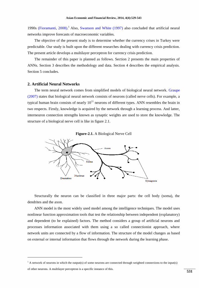
The term neural network comes from simplified models of biological neural network. Graupe

(2007) states that biological neural network consists of neurons (called nerve cells). For example, a

typical human brain consists of nearly 1011

neurons of different types. ANN resembles the brain in

two respects. Firstly, knowledge is acquired by the network through a learning process. And latter,

interneuron connection strengths known as synaptic weights are used to store the knowledge. The

structure of a biological nerve cell is like in figure 2.1.

Figure-2.1. A Biological Nerve Cell

Structurally the neuron can be classified in three major parts: the cell body (soma), the

dendrites and the axon.

ANN model is the most widely used model among the intelligence techniques. The model uses

nonlinear function approximation tools that test the relationship between independent (explanatory)

and dependent (to be explained) factors. The method considers a group of artificial neurons and

processes information associated with them using a so called connectionist approach, where

network units are connected by a flow of information. The structure of the model changes as based

on external or internal information that flows through the network during the learning phase.

1 A network of neurons in which the output(s) of some neurons are connected through weighted connections to the input(s)

of other neurons. A multilayer perceptron is a specific instance of this.


532

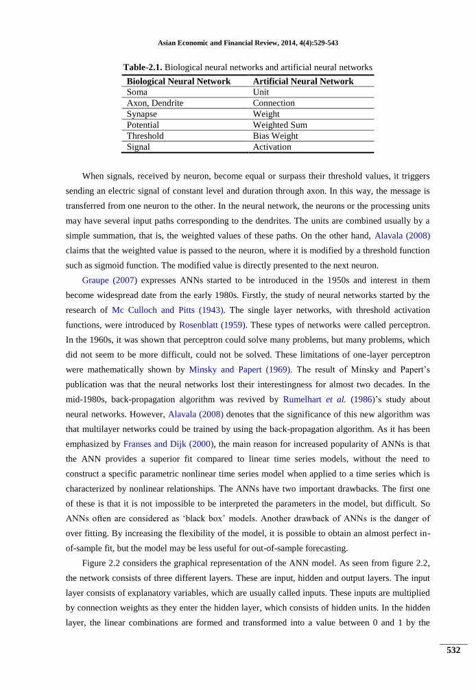
Table-2.1. Biological neural networks and artificial neural networks

Biological Neural Network Artificial Neural Network

Soma Unit

Axon, Dendrite Connection

Synapse Weight

Potential Weighted Sum

Threshold Bias Weight

Signal Activation

When signals, received by neuron, become equal or surpass their threshold values, it triggers

sending an electric signal of constant level and duration through axon. In this way, the message is

transferred from one neuron to the other. In the neural network, the neurons or the processing units

may have several input paths corresponding to the dendrites. The units are combined usually by a

simple summation, that is, the weighted values of these paths. On the other hand, Alavala (2008)

claims that the weighted value is passed to the neuron, where it is modified by a threshold function

such as sigmoid function. The modified value is directly presented to the next neuron.

Graupe (2007) expresses ANNs started to be introduced in the 1950s and interest in them

become widespread date from the early 1980s. Firstly, the study of neural networks started by the

research of Mc Culloch and Pitts (1943). The single layer networks, with threshold activation

functions, were introduced by Rosenblatt (1959). These types of networks were called perceptron.

In the 1960s, it was shown that perceptron could solve many problems, but many problems, which

did not seem to be more difficult, could not be solved. These limitations of one-layer perceptron

were mathematically shown by Minsky and Papert (1969). The result of Minsky and Papert‟s

publication was that the neural networks lost their interestingness for almost two decades. In the

mid-1980s, back-propagation algorithm was revived by Rumelhart et al. (1986)‟s study about

neural networks. However, Alavala (2008) denotes that the significance of this new algorithm was

that multilayer networks could be trained by using the back-propagation algorithm. As it has been

emphasized by Franses and Dijk (2000), the main reason for increased popularity of ANNs is that

the ANN provides a superior fit compared to linear time series models, without the need to

construct a specific parametric nonlinear time series model when applied to a time series which is

characterized by nonlinear relationships. The ANNs have two important drawbacks. The first one

of these is that it is not impossible to be interpreted the parameters in the model, but difficult. So

ANNs often are considered as „black box‟ models. Another drawback of ANNs is the danger of

over fitting. By increasing the flexibility of the model, it is possible to obtain an almost perfect in-

of-sample fit, but the model may be less useful for out-of-sample forecasting.

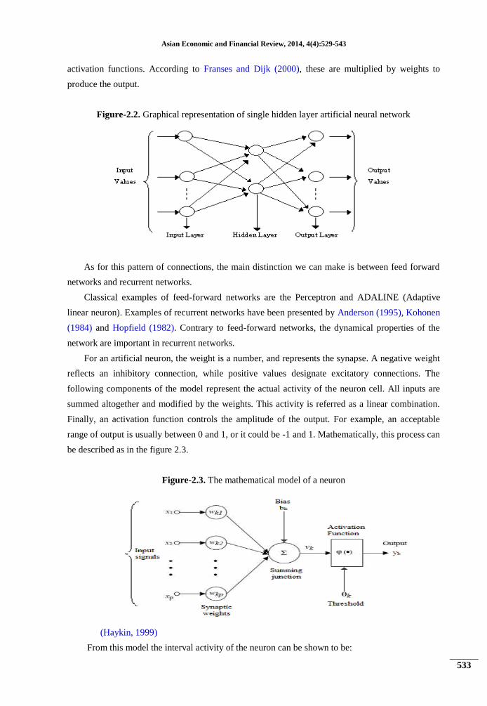
Figure 2.2 considers the graphical representation of the ANN model. As seen from figure 2.2,

the network consists of three different layers. These are input, hidden and output layers. The input

layer consists of explanatory variables, which are usually called inputs. These inputs are multiplied

by connection weights as they enter the hidden layer, which consists of hidden units. In the hidden

layer, the linear combinations are formed and transformed into a value between 0 and 1 by the


533

activation functions. According to Franses and Dijk (2000), these are multiplied by weights to

produce the output.

Figure-2.2. Graphical representation of single hidden layer artificial neural network

As for this pattern of connections, the main distinction we can make is between feed forward

networks and recurrent networks.

Classical examples of feed-forward networks are the Perceptron and ADALINE (Adaptive

linear neuron). Examples of recurrent networks have been presented by Anderson (1995), Kohonen

(1984) and Hopfield (1982). Contrary to feed-forward networks, the dynamical properties of the

network are important in recurrent networks.

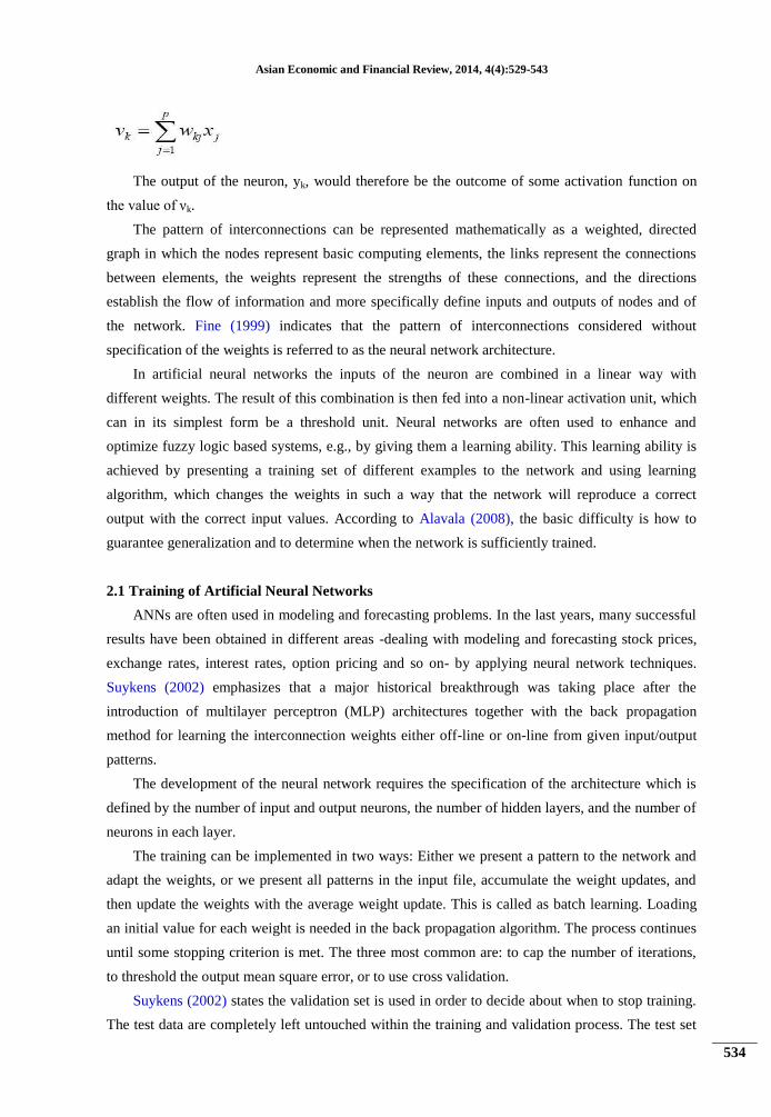
For an artificial neuron, the weight is a number, and represents the synapse. A negative weight

reflects an inhibitory connection, while positive values designate excitatory connections. The

following components of the model represent the actual activity of the neuron cell. All inputs are

summed altogether and modified by the weights. This activity is referred as a linear combination.

Finally, an activation function controls the amplitude of the output. For example, an acceptable

range of output is usually between 0 and 1, or it could be -1 and 1. Mathematically, this process can

be described as in the figure 2.3.

Figure-2.3. The mathematical model of a neuron

(Haykin, 1999)

From this model the interval activity of the neuron can be shown to be:


534

The output of the neuron, yk, would therefore be the outcome of some activation function on

the value of νk.

The pattern of interconnections can be represented mathematically as a weighted, directed

graph in which the nodes represent basic computing elements, the links represent the connections

between elements, the weights represent the strengths of these connections, and the directions

establish the flow of information and more specifically define inputs and outputs of nodes and of

the network. Fine (1999) indicates that the pattern of interconnections considered without

specification of the weights is referred to as the neural network architecture.

In artificial neural networks the inputs of the neuron are combined in a linear way with

different weights. The result of this combination is then fed into a non-linear activation unit, which

can in its simplest form be a threshold unit. Neural networks are often used to enhance and

optimize fuzzy logic based systems, e.g., by giving them a learning ability. This learning ability is

achieved by presenting a training set of different examples to the network and using learning

algorithm, which changes the weights in such a way that the network will reproduce a correct

output with the correct input values. According to Alavala (2008), the basic difficulty is how to

guarantee generalization and to determine when the network is sufficiently trained.

2.1 Training of Artificial Neural Networks

ANNs are often used in modeling and forecasting problems. In the last years, many successful

results have been obtained in different areas -dealing with modeling and forecasting stock prices,

exchange rates, interest rates, option pricing and so on- by applying neural network techniques.

Suykens (2002) emphasizes that a major historical breakthrough was taking place after the

introduction of multilayer perceptron (MLP) architectures together with the back propagation

method for learning the interconnection weights either off-line or on-line from given input/output

patterns.

The development of the neural network requires the specification of the architecture which is

defined by the number of input and output neurons, the number of hidden layers, and the number of

neurons in each layer.

The training can be implemented in two ways: Either we present a pattern to the network and

adapt the weights, or we present all patterns in the input file, accumulate the weight updates, and

then update the weights with the average weight update. This is called as batch learning. Loading

an initial value for each weight is needed in the back propagation algorithm. The process continues

until some stopping criterion is met. The three most common are: to cap the number of iterations,

to threshold the output mean square error, or to use cross validation.

Suykens (2002) states the validation set is used in order to decide about when to stop training.

The test data are completely left untouched within the training and validation process. The test set


535

is completely left untouched during the training and early stopping process and is used to check the

performance of the trained model on fresh data. Haykin (1999) describes that when the

performance starts to decline in the validation set, training should be stopped.

According to Principe et al. (1999); normalizing training data, using the tan h (hyperbolic

tangent) nonlinearity instead of the logistic function, setting the step size higher towards the input,

initializing the net‟s weights in the linear region of the nonlinearity, using more sophisticated

learning methods and always having more training patterns than weights will help decrease the

training times and, in generally, produce better performance.

The training algorithm is used to specify how the network should be trained. The type of

training and the optimization algorithm determine which the training options are available. The

type of training determines how the network processes the records. We can select one of the batch,

online and mini-batch training types to train the artificial neural networks in SPSS Neural

Networks 17.0 program.

2.2 Paradigms of Learning

The form of the relationships between the dependent and independent variables is determined

during the learning process. If a linear relationship between the dependent and independent

variables is fit, the results of the neural network should nearly approximate those of the linear

regression model. If a non linear relationship is more suitable, then the neural network will

automatically close the correct model structure. Yet, this flexibility has a trade off. This „trade off‟

is that synaptic weights are not easily interpretable. Thus, if it is important to explain the

relationship between the dependent and independent variables, it will be better to employ a more

traditional statistical model. Nonetheless, if model relatability is not important, it can be obtained

good model results more quickly applying a neural network.

We can categorize the learning situations in two distinct sorts. These are:

-Supervised learning or Associative learning in which the network is trained by providing it with

input and matching output patterns. These input-output pairs can be provided by a teacher, or by

the system, which contains the network.

-Unsupervised learning or Self-organization in which an output unit is trained to respond to clusters

of pattern within the input. In this paradigm the system is supposed to discover statistically salient

features of the input population. Alavala (2008) observes that unlike the supervised learning

paradigm, there is no a priori set of categories into which the patterns are to be classified.


536

3. METHODOLOGY AND DATA

Fine (1999) states that the neural networks methodology enables us to design useful nonlinear

systems accepting large numbers of inputs, with the design based solely on instances of input-

output relationships.

ANNs are more efficient when one or several layers of intermediate units are integrated in the

network. Input units send signals to these intermediate units located on one or several layers which

are said to be “hidden”. Intermediate layers of this sort are often called as hidden layers to

distinguish them from the input and output layers. Networks with one or several hidden layers are

referred to as multi layer ANNs. The most common multilayer ANN is the Multi layer Perceptron.

In this paper, we prefer to use the multilayer perceptron methodology to be built single hidden

layer feed forward model. The basic reasons that the multilayer perceptron methodology is to be

used are that the methodology is one of the most widely implemented neural network topologies

and provides very successful results. In this study, it is used 1992m1-2011m6 episode for

independent variables and 1992m2-2011m7 for dependent variable being consisted of the neural

network.

The multilayer perceptron is a function of predictors that minimize the prediction error of

dependent variable. Principe et al. (1999) indicate that two important characteristics of the

multilayer perceptron are: its nonlinear processing elements (PEs) which have a nonlinearity that

must be smooth (the logistic function and the hyperbolic tangent are the most widely used); and

their massive interconnectivity, i.e. any element of a given layer feeds all the elements of the next

layer.

According to Principe et al. (1999), MLPs are normally trained with the back propagation

algorithm). The back propagation rule propagates the errors through the network and allows

adaptation of the hidden PEs. The multilayer perceptron is trained with error correction learning,

which means that the desired response for the system must be known.

The multilayer perceptron with one hidden layer has the following form.

Perceptron learning rule suppose we have a set of learning samples consisting of an input vector

and a desired output. The perceptron learning rule can be stated as follows:

1. Start with random weights for the connections;

2. Select an input vector from the set of training samples;

3. If the perceptron gives an incorrect response, modify all connections;

4. And go back to second step.

A simple network is able to represent a relationship between the value of the output unit and the

value of the input units.

Crisis definitions have an important location being composed EWS. According to Edison

(2003), an EWS should consist of two components. The first of those is a precise definition of a

crisis and the second is a mechanism that will use the precise definition in order to generate

predictions of occurrences of a crisis. Both components are crucial to properly identifying a

currency crisis (Abiad, 2003).


537

It is possible to come across a great many of different crisis definitions in the literature of

empirical models of currency crisis. Different researchers have adopted alternative approaches to

the definition of a currency crisis.

For example, Frankel and Rose (1996) define a “currency crash” as a depreciation of the

nominal exchange rate of more than 25% that is also at least a 10% increase in the rate of nominal

depreciation from the previous year.

While some define a currency crisis solely on the basis of a substantial decline in the country‟s

nominal exchange rate, others; particularly Eichengreen et al. (1995), define a currency crisis as

one that exceeds an Index of Speculative Pressure (ISP) whose components include the changes in

the nominal exchange rate, and two other components which are frequently used by policymakers

for intervention to the movements in exchange rate, changes in interest rates and changes in

international reserves. The crisis measure, popularized by Eichengreen et al. (1995), defines an

“exchange market crisis” as occurring when their index of speculative pressure moves at least two

standard deviations above its mean.

Caramazza et al. (2000) also use an ISP for their crisis definition. The index is a weighted

average of detrended monthly exchange rate changes and reserve changes. The weights are chosen

so that the conditional variance of the two components of the index is equal, and trends are country

specific.

Glick and Moreno (1999) characterize crisis as percentage change in the exchange rate exceeds the

mean plus two standard deviations. Esquivel and Larrain (2000) use change in the real exchange

rate in their crisis definitions.

Kaminsky et al. (1998) and Goldstein et al. (2000) use an exchange market pressure index in

their crisis definitions. This index is composed as weighted average of month to month changes the

nominal exchange rate and reserve changes, where the threshold is plus 3 standard deviations away

from its mean; A sharp depreciation of the currency, a large decline in international reserves.

This study defines crisis in two ways. Firstly, it is composed of an exchange market pressure

index for the crisis definition, similarly the index in Kaminsky et al. (1998) and Goldstein et al.

(2000)‟s crisis definitions. Secondly, this study defines crisis episodes as departures of the actual

real Exchange rate from an estimated equilibrium real Exchange rate. Specifically, currency crisis

are defined as deviations of the actual exchange rate from a Hodric-Prescott filtered series. The

filtered series capture stochastic trends in the series and allows us to concentrate on the cyclical

behavior of potentially non-stationary real exchange rate series. It was used monthly data from

1990 to 2011 for Turkey in this model. It was reached similar findings with both methods also.

Thus, we assumed that the crisis continued from January to December of years in which it

appeared.

4. CASE: THE FORECASTING OF ECONOMIC/CURRENCY CRISIS

It was developed an ANN model that builds upon the multilayer perceptron to estimate crisis

episodes in this paper. We first define the multilayer perceptron with one hidden layer for this


538

model. There are 25 parameters in input layer. It has 7 neurons on its single hidden layer, and one

output unit which is only a scalar in output layer. A threshold neuron which has a constant input

that is equal to 1, is also defined. The observations are first divided into those observations in

periods of crises and observations of tranquil times. Crisis times are identified with a 1 while

tranquil times are identified with a 0.

Table-4.1. Artificial neural network architecture

1 Network‟s type Multilayer perceptron

2 Number of layers in the network 3

3 Number of neurons in the input layer 25 (excluding the bias unit)

4 Number of neurons in the hidden layer 7

5 Number of neurons in the output layer 2

6 Activation function used in the input

and output layers

Logistic

7 Rescaling method for covariates Standardized

8 Performance function Sum of squares error

9 Training type Batch

10 Optimization algorithm Gradient descent

11 Training options - Initial Learning Rate: 0.4

- Momentum: 0.8

12 Number of training epochs 1100

Table 4.1 shows fundamental elements used in artificial neural network architecture being

developed to estimate currency crisis happened in Turkey from 1990 to 2011.

Many transfer functions have been employed in ANN researches. The most popular of those are:

(1) Sigmoid (Logistic) function, γ(c) = 1/ (1+e-c

) and

(2) Hyperbolic tangent function, γ(c) =tanh(c) with tanh(c) = (ec -e

-c)/(e

c +e

-c).

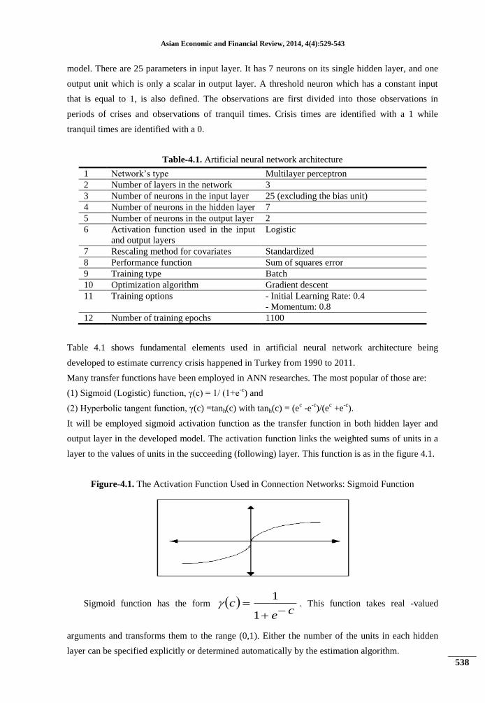
It will be employed sigmoid activation function as the transfer function in both hidden layer and

output layer in the developed model. The activation function links the weighted sums of units in a

layer to the values of units in the succeeding (following) layer. This function is as in the figure 4.1.

Figure-4.1. The Activation Function Used in Connection Networks: Sigmoid Function

Sigmoid function has the form ce

c

1

1 . This function takes real -valued

arguments and transforms them to the range (0,1). Either the number of the units in each hidden

layer can be specified explicitly or determined automatically by the estimation algorithm.


539

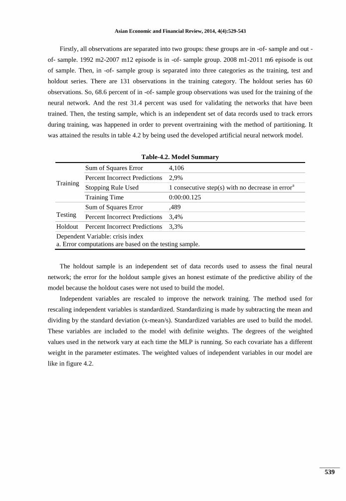
Firstly, all observations are separated into two groups: these groups are in -of- sample and out -

of- sample. 1992 m2-2007 m12 episode is in -of- sample group. 2008 m1-2011 m6 episode is out

of sample. Then, in -of- sample group is separated into three categories as the training, test and

holdout series. There are 131 observations in the training category. The holdout series has 60

observations. So, 68.6 percent of in -of- sample group observations was used for the training of the

neural network. And the rest 31.4 percent was used for validating the networks that have been

trained. Then, the testing sample, which is an independent set of data records used to track errors

during training, was happened in order to prevent overtraining with the method of partitioning. It

was attained the results in table 4.2 by being used the developed artificial neural network model.

Table-4.2. Model Summary

Training

Sum of Squares Error 4,106

Percent Incorrect Predictions 2,9%

Stopping Rule Used 1 consecutive step(s) with no decrease in errora

Training Time 0:00:00.125

Testing

Sum of Squares Error ,489

Percent Incorrect Predictions 3,4%

Holdout Percent Incorrect Predictions 3,3%

Dependent Variable: crisis index

a. Error computations are based on the testing sample.

The holdout sample is an independent set of data records used to assess the final neural

network; the error for the holdout sample gives an honest estimate of the predictive ability of the

model because the holdout cases were not used to build the model.

Independent variables are rescaled to improve the network training. The method used for

rescaling independent variables is standardized. Standardizing is made by subtracting the mean and

dividing by the standard deviation (x-mean/s). Standardized variables are used to build the model.

These variables are included to the model with definite weights. The degrees of the weighted

values used in the network vary at each time the MLP is running. So each covariate has a different

weight in the parameter estimates. The weighted values of independent variables in our model are

like in figure 4.2.


540

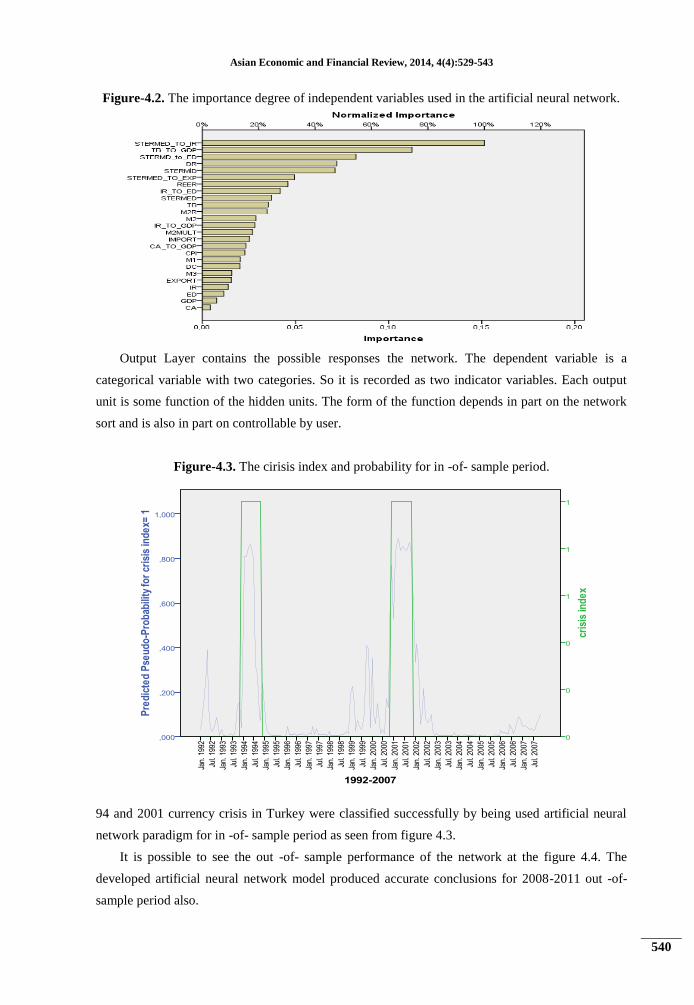
Figure-4.2. The importance degree of independent variables used in the artificial neural network.

Output Layer contains the possible responses the network. The dependent variable is a

categorical variable with two categories. So it is recorded as two indicator variables. Each output

unit is some function of the hidden units. The form of the function depends in part on the network

sort and is also in part on controllable by user.

Figure-4.3. The cirisis index and probability for in -of- sample period.

94 and 2001 currency crisis in Turkey were classified successfully by being used artificial neural

network paradigm for in -of- sample period as seen from figure 4.3.

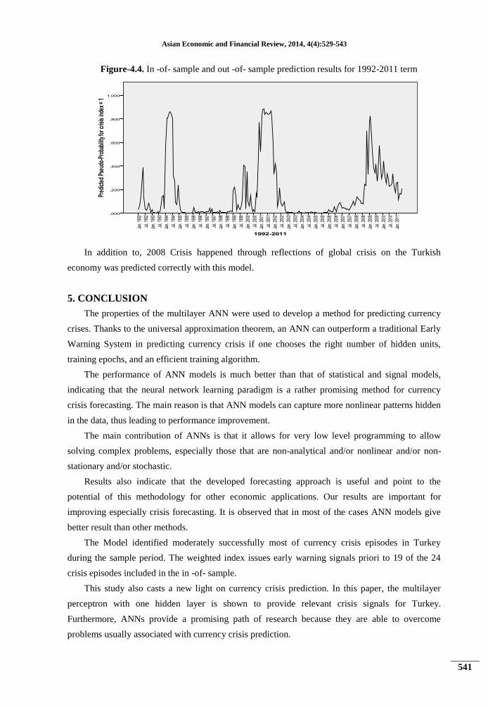
It is possible to see the out -of- sample performance of the network at the figure 4.4. The

developed artificial neural network model produced accurate conclusions for 2008-2011 out -of-

sample period also.


541

Figure-4.4. In -of- sample and out -of- sample prediction results for 1992-2011 term

In addition to, 2008 Crisis happened through reflections of global crisis on the Turkish

economy was predicted correctly with this model.

5. CONCLUSION

The properties of the multilayer ANN were used to develop a method for predicting currency

crises. Thanks to the universal approximation theorem, an ANN can outperform a traditional Early

Warning System in predicting currency crisis if one chooses the right number of hidden units,

training epochs, and an efficient training algorithm.

The performance of ANN models is much better than that of statistical and signal models,

indicating that the neural network learning paradigm is a rather promising method for currency

crisis forecasting. The main reason is that ANN models can capture more nonlinear patterns hidden

in the data, thus leading to performance improvement.

The main contribution of ANNs is that it allows for very low level programming to allow

solving complex problems, especially those that are non-analytical and/or nonlinear and/or non-

stationary and/or stochastic.

Results also indicate that the developed forecasting approach is useful and point to the

potential of this methodology for other economic applications. Our results are important for

improving especially crisis forecasting. It is observed that in most of the cases ANN models give

better result than other methods.

The Model identified moderately successfully most of currency crisis episodes in Turkey

during the sample period. The weighted index issues early warning signals priori to 19 of the 24

crisis episodes included in the in -of- sample.

This study also casts a new light on currency crisis prediction. In this paper, the multilayer

perceptron with one hidden layer is shown to provide relevant crisis signals for Turkey.

Furthermore, ANNs provide a promising path of research because they are able to overcome

problems usually associated with currency crisis prediction.


542

REFERENCES

Abiad, A., 2003. Early-warning systems: A survey and a regime-switching approach. IMF Working Paper.

No. 32.

Alavala, C.R., 2008. Fuzzy logic and neural networks: Basic concepts and application. New Age international.

Anderson, J.A., 1995. An introduction to neural networks. MIT press.

Brüggemann, A. and T. Linne, 2002. Are the central and eastern european transition countries still vulnerable

to a financial crisis? Results from the signals approach. BOFIT discussion papers. No.5.

Caramazza, F., R. Luca and R. Salgado, 2000. Trade and financial contagion in currency crises. IMF Working

Paper. No. 00155.

Edison, H.J., 2003. Do indicators of financial crises work? An evaluation of an early warning system.

International Journal of Finance and Economics 8(1): 11-53.

Edwards, S., 1989. Real exchange rates, devaluation, and adjustment: Exchange rate policy in developing

countries. MIT press.

Edwards, S. and J. Santaella, 1992. Devaluation controversies in the developing countries: Lessons from the

bretton woods era. In: A retrospective on the bretton woods system. Lessons for international

monetary reform. NBER working paper. No.4047.

Eichengreen, B., A. Rose and C. Wyplosz, 1995. Exchange market mayhem: The antecedents and aftermath of

speculative attacks. Economic Policy 10(21): 249-312.

Esquivel, G. and F. Larrain, 2000. Explaining currency crises. El Trimestre Economico 67(2): 191-237.

Fine, T.L., 1999. Feedforward neural network methodology. Springer-Verlag.

Fioramanti, M., 2008. Predicting sovereign debt crises using artificial neural networks: A comparative

approach. Journal of Financial Stability, 4(2): 149-164.

Franck, R. and A. Schmied, 2003. Predicting currency crisis contagion from east asia to russia and brazil: An

artificial neural network approach. AMCB Working Paper. No. 2. Bar-Ilan University.

Frankel, J. and A. Rose, 1996. Currency crashes in emerging markets: An empirical treatment. Journal of

International Economics, 43(3/4): 351-366.

Frankel, J. and G. Saravelos, 2010. Are leading indicators of financial crises useful for assessing country

vulnerability? Evidence from the 2008-09 global crises. NBER working paper. No. 16047.

Franses, P.H. and V.D. Dijk, 2000. Non-linear time series models in empirical finance. Cambridge University

Press.

Glick, R. and R. Moreno, 1999. Money and credit, competitiveness, and currency crises in Asia and Latin

America. FRBSF Pacific Basin Working Paper Series. No.99-01.

Goldstein, M., G.L. Kaminsky and C. Reinhart, 2000. Assessing financial vulnerability: An early warning

system for emerging markets. Peterson Institute Press.

Graupe, D., 2007. Principles of artificial neural networks 2nd Edn., World Scientific.

Haykin, S., 1999. Neural networks: A comprehensive foundation. Prentice Hall.

Hopfield, J.J., 1982. Neural networks and physical systems with emergent collective computational abilities.

Proceedings of National Academy of Science, 79(8): 2554-2558.


543

Kamin, S., 1988. Devaluation, external balance, and macroeconomic performance: A look at the numbers.

Department of Economics Princeton University.

Kaminsky, G.L., S. Lizondo and C.M. Reinhart, 1998. Leading indicators of currency crises. IMF Staff

Papers, 45(1): 1-48.

Kohonen, T., 1984. Self organization and associative memory. Springer-Verlag.

Mc Culloch, W.S. and W.H. Pitts, 1943. A logical calculus of the ideas immanent in nervous activity. Bulletin

of Mathematical Biophysics, 5(4): 115-133.

Minsky, M. and S. Papert, 1969. Perceptrons. MIT press.

Nag, A.K. and A. Mitra, 1999. Neural networks and early warning indicators of currency crisis. Reserve Bank

of India Occasional Papers, 20(2): 183-222.

Principe, J.C., W.C. Lefebvre and N R. Euliano, 1999. Neural and adaptive systems: Fundamentals through

simulations. John Wiley & Sons, Inc.

Rosenblatt, F., 1959. Two theorems of statistical seperability in the perceptron. In mechanisation of thought

processes. Proceeding of a Symposium Held at the National Physical Laboratory (1): 421-456.

Rumelhart, D.E., G.E. Hinton and W. R.J, 1986. Learning internal representation by error propagation (in

parallel distributed processing) MIT Press.

Sachs, J., A. Tornell and A. Velasco, 1996a. Financial crises in emerging markets: The lessons from 1995.

Brookings Papers on Economic Activity, 27(1): 147-216.

Sachs, J., A. Tornell and A. Velasco, 1996b. The mexican peso crisis: Sudden death or death foretold? Journal

of International Economics, 43(3/4): 265-283.

Suykens, J.A.K., 2002. Least squares support vector machines. World Scientific.

Swanson, N. and H. White, 1997. A model selection approach to real-time macroeconomic forecasting under

linear models and artificial neural networks. The Review of Economic and Statistics, 79(4): 540-

550.

an early warning system for turkey: the … 4(4)-529-543.pdf · asian economic and financial...

Documents