Lancaster University Management School

Working Paper 1996/004

An Earnings-Based Valuation Model in the Presence of Sustained Competitive Advantage

John O''Hanlon

The Department of Accounting and Finance Lancaster University Management School

Lancaster LA1 4YX UK

©John O''Hanlon All rights reserved. Short sections of text, not to exceed

two paragraphs, may be quoted without explicit permission, provided that full acknowledgement is given.

The LUMS Working Papers series can be accessed at http://www.lums.lancs.ac.uk

LUMS home page: http://www.lums.lancs.ac.uk/

AN EARNINGS-BASED VALUATION MODEL IN THE PRESENCE OF SUSTAINEDCOMPETITIVE ADVANTAGE

John O’Hanlon

Department of Accounting and Finance Lancaster UniversityLancaster LA1 4YX

U.K.

Telephone:(44) (0)1524-593631e-mail: J.O’hanlon@lancaster.ac.uk

29 September 1997

AcknowledgementsThe comments of Harold Bierman, Richard Brief, Colin Clubb, Gerald Feltham, Suresh Govindaraj,Richard Heaney, Yu Hon Lui, Jamie Munro, Ken Peasnell, Peter Pope, Andrew Stark and Paul Taylorare gratefully acknowledged.

An earnings-based valuation model in the presence of sustained competitive advantage

Abstract

In this paper, the process which generates a company’s economic value and its accounting numbers is

represented in terms of the company’s investment in, and utilisation of, competitive advantage. Within

this representation, it is shown that a company which earns normal economic returns might plausibly

generate perpetual exponential growth in positive net present value projects, in unrecorded goodwill and

in residual income. Since exponential growth in residual income may make it impracticable to construct

earnings-based valuation models which employ the time-series properties of unscaled residual income

(or of unscaled earnings), it is argued that earnings-based valuation models should employ the time-

series properties of scaled residual income (or of scaled earnings). A model which incorporates such

properties is then derived. In a certainty setting in which there are no shocks to the economic return

series, economic value is a function of normal profitability and of normal book value growth; in a setting

in which shocks to the economic return series occur, it is necessary to add a term which reflects

transitory abnormal profitability and a term which reflects transitory abnormal book value growth. The

importance of the abnormal profitability term is determined by persistence in abnormal profitability; the

importance of the abnormal book value growth term is determined by the normal market-to-book ratio.

1

1. Introduction

This paper represents the joint evolution of a company’s economic value and accounting numbers in

terms of the company’s investment in, and utilisation of, competitive advantage. In such a setting, the

company might plausibly experience persistent exponential growth in positive net present value (NPV)

projects, in unrecorded goodwill and in residual income. Since such growth in residual income may

make it impracticable to construct earnings-based valuation models which employ the time-series

properties of unscaled residual income (or of unscaled earnings), it is argued that earnings-based

valuation models should employ the time-series properties of scaled residual income (or of scaled

earnings). A model which incorporates such properties is then derived.

It is well known that economic value can be expressed as the sum of accounting book value and

the present values of all expected future residual incomes (Edwards and Bell, 1961; Edey, 1962;

Peasnell, 1982): the residual income component of the expression represents unrecorded goodwill.

Ohlson (1995) provided an important impetus to the modelling of the links between economic value and

accounting numbers by developing this residual income-based valuation relationship. Making the

assumptions that accounting book value is an unbiased estimator of economic value and that residual

income is generated by a zero-mean stationary time-series process, he derived a model in which

economic value is partly expressed as a weighted average of (i) book value and (ii) an ex-div earnings

multiple. The model provided an important illustration of how a theoretically supported accounting-

based valuation model could incorporate knowledge of the time-series properties of earnings. The

unrealistic assumption of unbiased accounting that was made in Ohlson (1995) was relaxed in Feltham

and Ohlson (1995) and in Feltham and Ohlson (1996). Feltham and Ohlson (1996) allowed persistent

unrecorded goodwill to arise from two sources which accountants might recognise intuitively: (i)

depreciation errors and (ii) the existence of a persistently growing stream of positive NPV projects, of

which the full value is not immediately captured by the balance sheet. Accounting-based valuation

models, such as that derived in Feltham and Ohlson (1996), which allow for the observable phenomenon

of persistent exponential growth in unrecorded goodwill to result from the observable phenomenon of

2

persistent streams of positive NPV projects, are attractive as potential bases for the practical task of

valuation and for the empirical research designs of market-based accounting researchers. However, there

is an apparent problem in modelling persistent growth in unrecorded goodwill in terms of persistent

growth in positive NPV projects: it is not clear how it can be expected that a persistently growing stream

of positive NPV projects will be generated in a competitive environment. Rappaport (1986) made the

point that competition should eventually eliminate the availability of positive NPV projects. This point

was echoed in studies by Bernard (1993) and by Ou and Penman (1993) which suggested that

competition is likely to eliminate positive NPV projects within a finite horizon and that, therefore, one

of the main potential causes of unrecorded goodwill and of positive residual income is likely to be

eliminated within such a horizon.

This paper addresses this issue by demonstrating that, even in a setting in which a company

does not earn abnormal economic returns, it is plausible that the company might be generating

persistently growing streams of positive NPV projects, of unrecorded goodwill and of residual income.

This demonstration rests upon a representation of the economic value and accounting numbers of a

going concern company as outputs of a process in which the company continually invests in, and

utilises, competitive advantage. The accounting depreciation is ‘correct’ in the sense that the rate

matches the rate of decline in project cash flows but it is ‘wrong’ in the sense that it ignores the value of

the competitive advantage that is embedded within projects. This representation provides indications as

to the impact of the acquisition and utilisation of competitive advantage upon the normal level of

profitability and upon the normal level of the market-to-book ratio. This representation is then

developed in order to derive an earnings-based valuation model which incorporates the time-series

properties of scaled earnings that might be observed in the setting described. Initially, the derivation is

effected in a certainty setting: the resultant model is similar to one which has appeared in the

shareholder value analysis literature, in which economic value is expressed in terms of normal

profitability and the normal book value growth rate. Subsequently, shocks to the economic return series

are incorporated: in the resultant model, economic value is expressed in terms of normal profitability,

3

the normal book value growth rate, transitory abnormal profitability and the transitory abnormal book

value growth rate.

The model, together with the underlying analysis, has a number of interesting features. First, it

expresses the central roles of the prediction of profitability and of the prediction of growth in the task of

fundamental analysis. 1 Second, it suggests a focus for literature that is concerned with the finite-horizon

properties of accounting numbers: it suggests that abnormal profitability and the abnormal book value

growth rate might plausibly be expected to approximate to zero within a finite horizon. Third, although

the analysis in this paper does not employ the technology of options theory, the representation

developed here provides some insight into the impact of real options (Dixit and Pindyck, 1994;

Trigeorgis, 1996) on items, such as profitability and the market-to-book ratio, which are of interest to

financial statement analysts. Fourth, the analysis gives indications of the effect of the acquisition and

utilisation of competitive advantage in determining the normal level of profitability. This is relevant for

those concerned with the use of managerial performance measures based on variants of residual income

such as Economic Profit (Copeland, Koller and Murrin, 1995; McTaggart, Kontes and Mankins, 1994)

and Economic Value Added (EVA®)2 (Stern, Stewart and Chew, 1995).

The remainder of this paper is organised as follows: section 2 shows that, within a setting in

which the company continually invests in competitive advantage, it is possible to accommodate a

persistent stream of positive NPV projects, with consequent exponential growth in unrecorded goodwill

and in residual income, without requiring that the company as a whole should earn abnormal economic

returns; section 3 derives an earnings-based valuation model which allows for such growth in

unrecorded goodwill and in residual income; section 4 concludes the paper.

2. Positive net present value projects, unrecorded goodwill, accounting rate of return and residual

income where payoffs from projects arise partly in the form of competitive advantage

1 The importance attached by analysts to the prediction of profitability and growth is evidenced by an account ofthe attitudes of successful analysts which was published by the London Sunday Times on 1 June 1997 (page 3 ofthe ‘Money’ section).2 EVA® is a service mark of Stern Stewart & Co. in the United States, the United Kingdom, and other countries ofthe world.

4

The analysis in this section of the paper is carried out in a no-arbitrage certainty setting in which the

company as a whole earns normal economic returns. Unrecorded goodwill, the accounting rate of return

(ARR) and residual income are represented as outputs of a process in which the going concern company

continually makes investments in competitive advantage which is embedded within projects. The

company makes an initial investment in a zero NPV first generation project of which the payoffs accrue

partly in the form of direct cash receipts and partly in the form of competitive advantage. This

competitive advantage is realised as positive NPV second generation projects. Investment in these

second generation projects itself results in subsequent payoffs which accrue partly as direct cash receipts

and partly as positive NPV third generation projects. This process continues indefinitely, with the

company continually ‘cashing in’ previously acquired competitive advantage through investment in

positive NPV projects which themselves deliver competitive advantage which will bring about

subsequent positive NPV projects. The accounting system depreciates the competitive advantage along

with the projects in which it is embedded.

It is shown that, within the framework represented here, persistent exponential growth in

positive NPV investments, in unrecorded goodwill and in residual income might plausibly arise even in

the absence of abnormal economic returns for the company as a whole. It is also shown that the

asymptotic levels of ARR and of the market-to-book ratio are functions of parameters which capture (i)

the proportion of total project value that is represented by investment in competitive advantage and (ii)

the proportion of the cost of new projects that is represented by the ‘cashing in’ of previously acquired

competitive advantage. The following assumptions are made regarding the analysis in this section:

i. At incorporation (time 0), the company makes an initial issue of equity capital which is wholly

invested in the company's first generation project. The amount of equity capital raised is the

opening book value of the company (y0). Abnormal economic returns for the company are

precluded from this part of the analysis, so the first generation project has zero NPV: the

economic value of the company at time 0 (P0) is equal to y0. (If the first generation project is

allowed to have a non-zero NPV, this does not change the asymptotic results derived below.)

5

ii. The periodic payoffs from the first generation zero NPV project each accrue partly in the form

of cash receipts directly attributable to that project and partly in the form of positive NPV

second generation projects which result from competitive advantage acquired through

investment in that first generation project. These second generation projects partly consist of an

investment in competitive advantage. The payoffs from the second generation projects therefore

also accrue partly in the form of cash receipts and partly in the form of third generation positive

NPV projects: the process continues indefinitely. This process is characteristic of a company

which is in the going concern phase of its existence. That part of the total period t payoff of the

company which accrues in the form of cash at period t is denoted by Ct; that part of the period t

payoff which accrues in the form of positive NPV projects at period t is denoted by Nt. The

proportion of total payoffs which accrues in the form of cash receipts is denoted by F. F is

assumed to be constant across all projects and across time. Some, but not all, of project payoffs

are assumed to arise as cash receipts: therefore, 0 < F < 1. For all t,

F C C Nt t t= +/ ( ) . (1)

The proportion of total project payoffs which accrues as positive NPV projects arising from

earlier investment in competitive advantage is (1-F). Thus, (1-F) represents the proportion of the

value of projects which is made up of the investment in competitive advantage.

iii. The total cash cost of buying into all of the second and subsequent generation projects that arise

at period t is denoted by It. The ratio of cash cost to present value of such new projects is

denoted by H. As with F, H is assumed to be constant across all projects and across time. All

second and subsequent generation projects are assumed to be positive NPV projects with an

initial cash cost of greater than 0: therefore, 0 < H < 1. (1-H) represents the ratio of NPV to

present value of second generation and subsequent projects. H/(1-H) therefore represents the

ratio of cash cost to NPV of such projects. Consequently for all t:

I NH

Ht t=−

1

. (2)

6

Where the company as a whole is earning normal economic returns, (1-H) represents the

proportion of the total value of second generation and subsequent projects that is contributed by

the utilisation of competitive advantage embedded within earlier projects.

iv. Each project generates a stream of total periodic payoffs (i.e. C plus N) which accrues in the

form of a declining perpetuity, where the rate of decline is B per period. 0 < B ≤ 1. The use of

this assumed payoff pattern is convenient because it produces a relatively simple analysis.

However, there is empirical evidence to support the use of such a pattern. As will become

apparent later, this declining payoff pattern gives rise to a profitability persistence parameter in

the form of the autoregressive coefficient of an autoregressive process of order 1 (AR(1)

process): empirical evidence in O’Hanlon (1996) suggests that, of various standard time-

series generating processes, AR(1) is the one which best characterises ARR series in the U.K.

v. There are no financial assets, financial liabilities or working capital at any period end. The

dividend for period t, denoted by dt, is the excess of the cash receipts from projects for that

period over the cash cost of investment in new projects for that period:

d C It t t= − . (3)vi. Each project is recorded in the balance sheet at its historic cash cost less accumulated

accounting depreciation. The accounting depreciation rate for all projects is determined by the

rate of decline in the projects' cash payoff stream. The rate is therefore B per period on a

declining balance basis. The depreciation is ‘correct’ in that the rate matches the rate of decline

in project cash flows but is ‘wrong’ in that it ignores the value of the competitive advantage

embedded within projects:3 the investment in this competitive advantage is depreciated as part

of the projects within which it is embedded, rather than being capitalised in anticipation of the

subsequent positive NPV projects to which it will give rise. This non-recognition (‘over-

depreciation’) by the accounting system of the valuable competitive advantage gives rise to a

market-to-book premium.

3 A further complication could be introduced by allowing the depreciation rate to differ from the rate of declinein cash flows: this complication is not introduced here.

7

vii. Accounting obeys the clean surplus relationship:

y y x dt t t t= + −−1 , (4)

where yt (yt-1) is the accounting book value at period end t (t-1) and xt is accounting earnings for

period t, where xt = Ct - yt-1B.

Before proceeding with the analysis, two points are made. First, given the no-arbitrage certainty

setting, the dollar return is as follows for all t:

( ) ,R P P P d P P C It t t t t t t t− = − + = − + −− − −1 1 1 1 (5)

where R is one plus the cost of equity, which is assumed to be constant, and Pt (Pt-1) is the economic

value of equity capital at period-end t (t-1). Pt can be written as the present value at period-end t of the

projects which made up Pt-1 plus the present value of new projects arising at period t:

P P B N It t t t= − + +−1 1( ) . (6)

Combining (5) and (6), the dollar return for period t can be written as the period t total payoff (Ct plus

Nt) less the decline during period t in the present value of the projects which made up Pt-1:

( ) .R P N C P Bt t t t− = + −− −1 1 1 (7)

Second, it is important to comment on the term ‘positive NPV’ which is used above and in the following

analysis. If the definition of ‘cost’ is amplified to include the value of the previously acquired

competitive advantage that is being ‘cashed in’ to provide positive NPV projects, these projects are not

positive NPV at all: they just appear to be positive NPV because standard capital budgeting procedures

ignore the value of the competitive advantage that is being utilised. The impression that these projects

have positive NPV is reinforced by the accounting depreciation procedure which ‘over-depreciates’ the

investment in competitive advantage, with the consequence that the book value of second and

subsequent generation projects is less than their present value. In this setting, the standard capital

budgeting procedures and the standard accounting depreciation procedures conspire together to make

projects look as though their present value exceeds their cost. Such a process is likely to be present in

the return-earnings generating process of any going concern business and is at the heart of the

8

subsequent exposition. For the sake of terminological convenience, and to be consistent with other

studies which allow for such processes (e.g. Feltham and Ohlson (1996)), I will continue to use the term

‘positive NPV’ in the exposition.

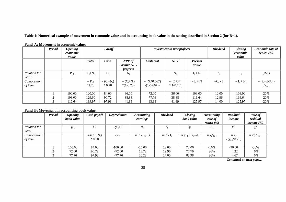
In order to facilitate understanding of the setting described above, Table 1 presents a numerical

example of the evolution of economic value and accounting numbers in that setting. In this example, R =

1.20, F = 0.70, H = 0.667 and B = of 1.00. Making B equal to 1.00, gives a particularly simple example.

Table 1 contains the following notation not previously defined in the text: At (= xt/yt-1) denotes the ARR

for period t, xat (= xt - (R-1)yt-1) denotes residual income for period t and χ ta denotes the rate of residual

income for period t ( = xat / yt-1).

(INSERT TABLE 1 ABOUT HERE)

The subsequent analysis within this section is presented in the form of three propositions.

Proposition 1 suggests that, in the setting described above, economic value and investment in positive

NPV projects might plausibly grow exponentially. It is shown that the rate of growth is a function of R,

F, B and H. Proposition 2 states that the asymptotic rate of growth in book value and in unrecorded

goodwill is the same as the rate of growth in economic value defined in Proposition 1. It is shown that

the asymptotic market-to-book ratio is the reciprocal of H. Finally, Proposition 3 states that unscaled

residual income grows exponentially at the rate of growth in book value defined in Proposition 2. On the

basis of these three propositions, it is argued that earnings-based valuation models incorporating time-

series properties of earnings should reflect the exponential growth property of accounting numbers that

is likely to be observed in the presence of continual investment in competitive advantage.

9

Proposition 1: In the absence of abnormal economic returns, the rate of growth in economic value and

in new investment in positive NPV projects is a weighted average of (R-1) and (-B), where the weights

reflect the relative proximity of F to 1 and H respectively. If dividends are positive, positive exponential

growth in economic value and in new investment in positive NPV projects occurs if (R-1)(1-F)/(F-H)

exceeds B. Such growth does not depend upon the presence of abnormal economic returns.

Proof: From (2) and (3), the dividend yield at period t (= dt/Pt-1), denoted by Dt, is

DC N H H

Ptt t

t

=− −

−

( / ( )).

1

1

(8)

Substitution of (1) into (7) gives

C P R B F

N P R B Ft t

t t

= − += − + −

−

−

1

1

1

1 1

( )

( ) ( ) .(9)

Substitution of (9) into (8) gives

DP R B F P R B F H H

P

R BF H

H

tt t

t

=− + − − + − −

= − + −−

− −

−

1 1

1

1 1 1 1

11

( ) ( ) ( ) ( / ( ))

( ) .

(10)

R, B, F and H are constant, so Dt (hereafter D) is constant. (Note here that positive dividends

require F > H.) The rate of growth in economic value, denoted by g , is constant at

g R D RF

HB

F H

H= − − = − −

−

− −−

( ) ( ) .1 11

1 1(11)

From (11), g is a weighted average of (R-1) and (-B), where the weights reflect the relative

proximity of F to 1 and H respectively.4 If dividends are positive (i.e. if F > H), positive

exponential growth in P occurs if (R-1)(1-F)/(F-H) > B. From (9), Nt is proportional to Pt-1.

Therefore, such growth in N also occurs if (R-1)(1-F)/(F-H) > B. Positive exponential growth in

P and in N does not depend upon the existence of abnormal economic returns. n

4 Note that as F approaches 1, little of the payoff from projects accrues as competitive advantage, retentionsapproach zero and g approaches -B; as F falls towards H, the proportion of payoffs that accrues in the form of cash

falls towards the proportion of new project value that is made up of cash cost: payout approaches zero andg approaches (R-1).

10

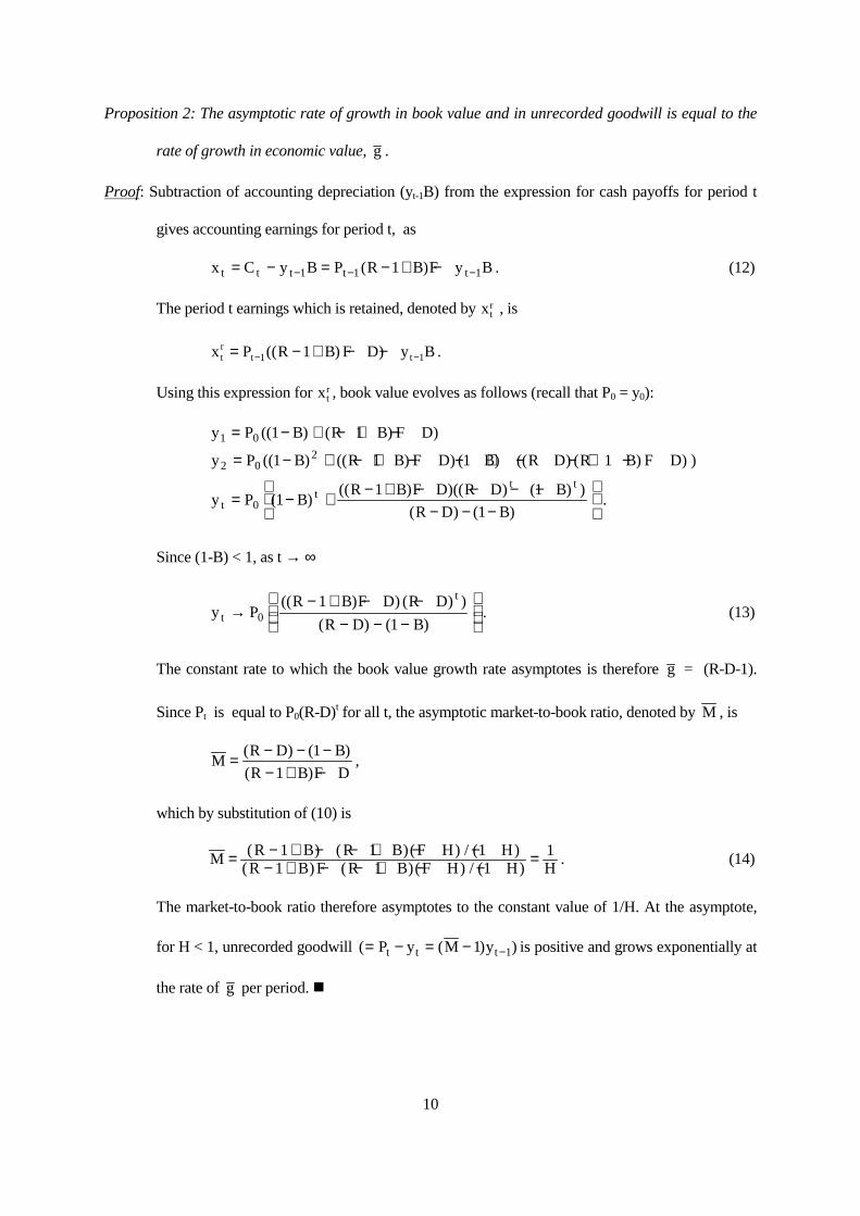
Proposition 2: The asymptotic rate of growth in book value and in unrecorded goodwill is equal to the

rate of growth in economic value, g .

Proof: Subtraction of accounting depreciation (yt-1B) from the expression for cash payoffs for period t

gives accounting earnings for period t, as

x C y B P R B F y Bt t t t t= − = − + −− − −1 1 11( ) . (12)

The period t earnings which is retained, denoted by xtr , is

x P R B F D y Btr

t t= − + − −− −1 11(( ) ) .

Using this expression for xtr , book value evolves as follows (recall that P0 = y0):

y P B R B F D

y P B R B F D B R D R B F D

y P BR B F D R D B

R D Btt

t t

1 0

2 02

0

1 1

1 1 1 1

11 1

1

= − + − + −

= − + − + − − + − − + −

= − + − + − − − −− − −

(( ) ( ) )

(( ) (( ) ) ( ) (( ) ( ) ) )

( )(( ) )(( ) ( ) )

( ) ( ).

Since (1-B) < 1, as t → ∞

y PR B F D R D

R D Bt

t

→− + − −

− − −

0

1

1

(( ) ) ( ) )

( ) ( ). (13)

The constant rate to which the book value growth rate asymptotes is therefore g = (R-D-1).

Since Pt is equal to P0(R-D)t for all t, the asymptotic market-to-book ratio, denoted by M , is

MR D B

R B F D= − − −

− + −( ) ( )

( ),

1

1

which by substitution of (10) is

M R B R B F H HR B F R B F H H H

= − + − − + − −− + − − + − − =( ) ( )( ) / ( )

( ) ( )( ) / ( ).1 1 1

1 1 11 (14)

The market-to-book ratio therefore asymptotes to the constant value of 1/H. At the asymptote,

for H < 1, unrecorded goodwill ( ( ) )= − = − −P y M yt t t1 1 is positive and grows exponentially at

the rate of g per period. n

11

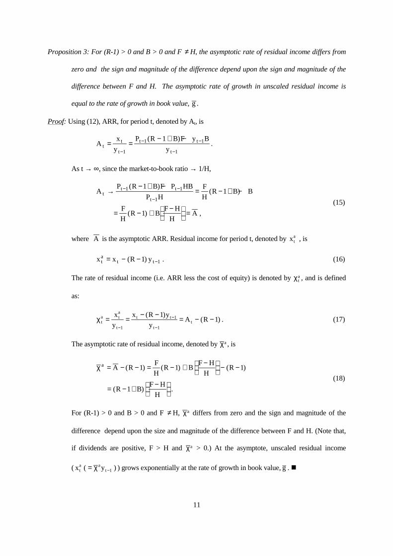
Proposition 3: For (R-1) > 0 and B > 0 and F ≠ H, the asymptotic rate of residual income differs from

zero and the sign and magnitude of the difference depend upon the sign and magnitude of the

difference between F and H. The asymptotic rate of growth in unscaled residual income is

equal to the rate of growth in book value, g .

Proof: Using (12), ARR, for period t, denoted by At, is

Ax

y

P R B F y B

ytt

t

t t

t

= =− + −

−

− −

−1

1 1

1

1( ).

As t → ∞, since the market-to-book ratio → 1/H,

AP R B F P HB

P H

F

HR B B

F

HR B

F H

HA

tt t

t

→− + −

= − + −

= − + −

=

− −

−

1 1

1

11

1

( )( )

( ) ,

(15)

where A is the asymptotic ARR. Residual income for period t, denoted by xta , is

x x R yta

t t= − − −( ) .1 1 (16)

The rate of residual income (i.e. ARR less the cost of equity) is denoted by χta , and is defined

as:

χ ta t

a

t

t t

tt

x

y

x R y

yA R= =

− −= − −

−

−

−1

1

1

11

( )( ) . (17)

The asymptotic rate of residual income, denoted by χa , is

χ a A RF

HR B

F H

HR

R BF H

H

= − − = − + −

− −

= − + −

( ) ( ) ( )

( ) .

1 1 1

1

(18)

For (R-1) > 0 and B > 0 and F ≠ H, χa differs from zero and the sign and magnitude of the

difference depend upon the size and magnitude of the difference between F and H. (Note that,

if dividends are positive, F > H and χa > 0.) At the asymptote, unscaled residual income

( x yta a

t( )= −χ 1 ) grows exponentially at the rate of growth in book value, g . n

12

The propositions that have been developed in this section suggest how residual income might be

expected to evolve through time in the case of a going concern company which is continually investing

in competitive advantage. Even in a situation in which the company as a whole is earning normal

economic returns only, one might expect to observe exponential growth in economic value, in positive

NPV projects, in book value, in unrecorded goodwill and in residual income. The process by which

investment in one project generates competitive advantage that can be exploited through investment in

subsequent projects is a fundamental determinant of the way in which going concern companies evolve.

(“Learning by doing” is an example of a phenomenon which results in investment in competitive

advantage being bundled up with other outlays and expensed in the going concern company.) This

process is therefore likely to be a fundamental determinant of the joint evolution of economic value,

book value and accounting earnings. Attempts to analyse the joint evolution of economic value, book

value and accounting earnings might therefore benefit from an accounting-based valuation model that

explicitly allows for the behaviour of accounting numbers that is likely to be observed in the presence of

continual investment in competitive advantage. The following section develops an earnings-based

valuation model which allows for the exponential growth in residual income that might be observed in

the presence of such sustained competitive advantage.

Before proceeding further with the analysis, it is instructive to dwell briefly on some of the

implications of expressions (15) and (18). These expressions suggest that, in the presence of sustained

competitive advantage, where accounting depreciation does not separately recognise investment in that

competitive advantage, normal profitability and ‘normal excess profitability’ are a function of the

investment in, and utilisation of, competitive advantage: for F > H, the normal excess of profitability

over the cost of equity is a positive function of R, B and F and is a negative function of H. This result

has implications in two related contexts. First, although the analysis in this paper does not employ the

technology of options theory, the acquisition and utilisation of competitive advantage is essentially

about the acquisition and utilisation of real options. The representation that is developed here provides

an indication of how the acquisition and utilisation of real options (Dixit and Pindyck, 1994; Trigeorgis,

13

1996) might impact on items, such as profitability and the market-to-book ratio, which are of interest in

financial statement analysis. Second, the analysis is relevant for those concerned with the

implementation of managerial performance measurement systems based on variants of residual income.

Such variants include Economic Profit (Copeland, Koller and Murrin, 1995; McTaggart, Kontes and

Mankins, 1994) and Economic Value Added (EVA®) (Stern, Stewart and Chew, 1995). Economic Profit

and EVA® are variants of residual income in which certain ‘accounting distortions’ are corrected: the

intention is that the resulting adjusted residual income measure can be used such that positive (negative)

residual income indicates superior (inferior) economic performance. As can be seen from expressions

(15) and (18), the interaction of F and H can produce a normal rate of residual income of greater than

zero. To the extent that the accounting corrections do not deal with the phenomenon represented here,

positive residual income may not necessarily be an indicator of superior economic performance: it may

be incorrect to regard a positive or negative value for residual income as an indication of positive or

negative abnormal performance.5

3. An earnings-based valuation model where payoffs from projects accrue partly in the form of

competitive advantage

Section 2 shows that unscaled residual income might plausibly grow exponentially at the book value

growth rate. Standard autoregressive, integrated moving average (ARIMA) time-series modelling

techniques involve the transformation through differencing of a series to a stationary series and then the

estimation of the autoregressive and moving average parameters for the appropriately differenced series.

If the series exhibits exponential growth, differencing may fail to achieve stationarity. Attempts to use

ARIMA-based approaches for the estimation of residual income persistence (or, for similar reasons, for

the estimation of earnings persistence) on the basis of unscaled data may fail or may result in the

identification of generating processes with unnecessarily high orders of differencing. For reasons related

5 The need to set benchmarks of other than zero for residual income and its variants is recognised by SternStewart & Co., who market the EVA® variant of residual income. In setting EVA® benchmarks, the differencebetween market value and (adjusted) book value is sometimes used as a basis for imputing expectations of future(non-zero) EVA®. I am grateful to Joel Stern for this information.

14

to those outlined in Section 2, stock price changes are also likely to exhibit exponential growth.

However, whilst the Finance literature has long acknowledged that work involving the time-series

properties of stock price changes should focus on scaled changes, it is not widely acknowledged that

work on the time-series properties of accounting flows should focus on the time-series properties of the

scaled flows. On the basis of the analysis in section 2, it is argued that theoretical or empirical earnings-

based valuation models which incorporate the time-series properties of residual income should focus on

scaled residual income and that, since the driver of growth in residual income is book value, the

appropriate scaling item is book value. The remainder of this section is concerned with the construction

of a model based on residual income scaled by book value.

Peasnell (1982) showed that, if accounting obeys the clean surplus relationship, the dividend

capitalisation model,

P E d Rt t t= +=

∞−∑ ( ) ,τ

τ

τ

1

(19)

where E (.) is an expectations operator, can be re-written as

P y E x Rt t t ta= + +

=

∞−∑ ( ) .τ

τ

τ

1

(20)

Appendix 1 shows that, in a certainty setting where there have been no shocks to the economic rate of

return series and where xa and y will grow at the constant rate of (R-D-1) = g , (20) can be re-written as

P yA g

t t=−−

−1 1γ

, (M.1)

where γ = +R g/ ( )1 . This is a no-shock accounting-based valuation model, containing a normal ARR

term and a normal book value growth rate term. (M.1) can also be written as

P yA g

R gt t= −− −

( ),

1

which is described as the ‘equity spread’ model in a shareholder value analysis text by McTaggart,

Kontes and Mankins (1994).

15

The effect of past and current shocks to the economic rate of return series is now overlaid upon

the no-shock accounting-based valuation model, (M.1). (M.1) is written in terms of normal profitability

and the normal book value growth rate: allowance for shocks requires the addition of terms which deal

with transitory abnormal profitability and the transitory abnormal book value growth rate. In permitting

shocks to the economic rate of return series, the analysis is moving from a certainty setting to an

uncertainty setting. In such a setting, the values of the future payoffs (C plus N) from projects are

expected values rather than certain values. The investment of It at period t becomes an investment in the

cash payoffs from a group of projects plus an investment in a basket of options embedded within that

group of projects. The present value at period-end t of the expected cash payoffs from that group of

projects and of the expected expiration values of the embedded options, taken together, is It / H (i.e. the

cash cost of the projects times the ratio of present value to cost).

In developing (M.1) to allow for present and past shocks, it is assumed that the company has

reached its asymptotic values of ARR ( A ), market-to-book ratio ( M ) and book value growth rate ( g )

and has previously encountered no shocks to its economic return series. It then experiences a shock to its

economic return series which represents the effect of a revision concerning the total payoffs (i.e. C plus

N) expected to accrue from the company’s existing projects. The changes to the expected payoffs which

represent the shock are capitalised as a declining perpetuity. Such a shock causes the economic rate of

return to diverge from (R-1) in the period in which the shock arises. Market efficiency is assumed:

consequently, the economic rate of return is expected to be (R-1) in all periods subsequent to the period

in which the shock arises. The parameters, F, B and H, are assumed to remain constant in the aftermath

of the shock, as is the cost of equity, (R-1). Furthermore, it is assumed that the accounting depreciation

policy does not change in response to the shock: consequently, it takes time for the impact of the

economic income shock to be captured by the accounting system and there results time-series

dependence (persistence) in the ARR series. Accounting continues to obey the clean surplus

relationship. In Appendix 2 it is shown that this set of circumstances gives rise to the following

accounting-based valuation model:

16

P yA g

A A g gM

t t t t=−−

+ −−

+ −−

−

−1 1γ

ωγ ω

γ ωγ ω

( ) ( ) , (M.2)

where ( )A At − is the transitory abnormal ARR, g is now defined to be the normal book value growth

rate, ( )g gt − is the transitory abnormal book value growth rate and ω is the asymptotic persistence

parameter for abnormal ARR, for the abnormal rate of residual income and for the abnormal book value

growth rate. As stated in Appendix 2, the persistence parameter, ω , takes the form of the autoregressive

coefficient that would be estimated in an autoregressive model of order 1 (AR(1) model) for each of

these items. The definition of the persistence parameter in terms of an AR(1) coefficient results from the

underlying assumption that payoffs take the form of a declining perpetuity.6 (M.2) is consistent with a

version of equation (3.a) from Feltham and Ohlson (1996) in which cash flow decline is set equal to the

reducing balance depreciation rate.7

According to (M.2), the value of equity is obtained by adjusting the steady state model (M.1),

which contains a normal ARR term and a normal book value growth rate term, by a term reflecting

temporary divergence from normal ARR and by a term reflecting temporary divergence from the normal

book value growth rate. The multiplier on the abnormal ARR term comprises the growth adjusted

discount factor and the asymptotic ARR persistence parameter, ω : as ω approaches zero, the multiplier

on abnormal ARR approaches zero. The multiplier on the abnormal book value growth rate term also

includes these two terms but the key component of this multiplier is the asymptotic market-to-book ratio

M (=1/H, where H < 1). As H (= the ratio of cost to present value of new projects) falls, the multiplier

on the abnormal book value growth rate diverges positively from one.

(M.2) does not include an ‘other information’ term, such as that included in the Ohlson (1995)

analysis, which captures the effect on the economic value of the company of that information which has

not yet impacted on accounting numbers and which is not captured by persistence multipliers applied to

6 As was mentioned earlier, empirical evidence in O’Hanlon (1996) suggests that, of various standard time seriesprocesses, AR(1) is the one which best characterises ARR series in the U.K..7 The lengthy but straightforward demonstration of the consistency is not reproduced here but is available on requestfrom the author.

17

current accounting numbers. In an empirical setting, this consideration may be important but no attempt

is made here to include such a term. Such a term would be compound function of the stochastic

properties of accounting numbers and of the stochastic properties of ‘other information’:8 it is not clear

that the precise form of such a term would add significantly to the insights afforded by this analysis and,

consequently, it is omitted.

As well as suggesting how the time-series properties of earnings might be incorporated into

earnings-based valuation models in the setting described, (M.2) has a number of additional interesting

features. First, it expresses the central roles of the prediction of profitability and of the prediction of

growth in the task of fundamental analysis. Second, it suggests a focus for literature concerned with the

finite-horizon properties of accounting numbers. Examples of such literature include Bernard (1993) and

Ou and Penman (1993). Under the conditions described in this paper, where persistent streams of

positive NPV projects are generated, it is plausible to expect that unscaled residual income will not

approximate to zero within a finite horizon. However, where the normal characteristics of the company's

projects (denoted here by R, B, F, H) do not change, it is plausible to expect that the abnormal ARR and

the abnormal book value growth rate will approximate to zero over such a horizon. Therefore, the

development of models based on finite horizon properties of accounting might usefully focus on

abnormal ARR and on the abnormal book value growth rate. Furthermore, the underlying analysis

provides an indication of the impact of the acquisition and utilisation of competitive advantage on

normal profitability levels. This is of potential relevance both for those concerned with the impact of

real options on financial statement items and for those concerned with the use of residual income, and

its variants, as measures of managerial performance.

4. Conclusion

This paper represents the joint evolution of economic value, accounting book value and accounting

earnings as the product of a process in which investments by companies include investment in

competitive advantage which gives rise to future positive NPV projects. The depreciation is ‘correct’ in

8 See Ohlson (1995) for an example of the form of such an ‘other information’ term.

18

the sense that the rate matches the rate of decline in project cash flows but is ‘wrong’ in the sense that it

ignores the value of the competitive advantage that is embedded within projects. This process may give

rise to perpetual exponential growth in the generation of positive NPV projects, in unrecorded goodwill

and in residual income, even in the absence of abnormal economic returns for the company as a whole.

Since such growth would make it difficult to exploit the time-series properties of unscaled residual

income (or of unscaled earnings) in earnings-based valuation models, it is argued that earnings-based

valuation models should employ the time-series properties of residual income scaled by book value (or

of total earnings scaled by book value). The paper then derives such a valuation model. The model

incorporates normal profitability, transitory abnormal profitability, the normal book value growth rate

and the transitory abnormal book value growth rate. The multiplier on abnormal profitability is driven

by persistence in abnormal profitability; the multiplier on the abnormal book value growth rate is driven

by the normal market-to-book ratio. The model expresses the central roles of the prediction of

profitability and of the prediction of growth in the task of fundamental analysis and suggests a focus for

literature that is concerned with the finite-horizon properties of accounting numbers. Furthermore, the

underlying analysis provides an indication of the impact of the acquisition and utilisation of competitive

advantage on normal profitability levels and on normal market-to-book levels.

The analysis in this paper contains a number of simplifying features which indicate directions in

which this type of analysis might be developed both empirically and theoretically. First, it is assumed

that the required return and payoff characteristics (R, F, B and H) of all projects are constant both across

projects and through time: allowance for cross-sectional and time-series variation in these parameters

might prove to be important in an empirical setting. Second, it is assumed that the payoffs from projects

take the form of a declining perpetuity. Although there is some empirical justification for this

simplifying assumption, it may not hold in all settings: different payoff patterns would give rise to

different multipliers on the terms in the model. Third, it could be argued that the model presented in this

paper should be augmented by an ‘other information’ term, such as that included in the Ohlson (1995)

analysis. In an empirical setting, this consideration may be important but no attempt is made here to

19

include such a term. Fourth, although this paper affords some insights as to the impact of real options on

items such as profitability and the market-to-book ratio, it does not employ the technology of options

theory to represent the process: there is much scope for the exploration of the impact of real options on

the properties of financial statement items which are used for valuation purposes.

20

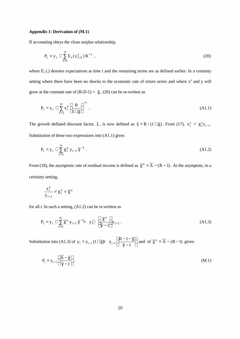
Appendix 1: Derivation of (M.1)

If accounting obeys the clean surplus relationship,

P y E x Rt t t ta= + +

=

∞−∑ ( ) ,τ

τ

τ

1

(20)

where Et (.) denotes expectations at time t and the remaining terms are as defined earlier. In a certainty

setting where there have been no shocks to the economic rate of return series and where xa and y will

grow at the constant rate of (R-D-1) = g , (20) can be re-written as

P y xR

gt t ta= +

+

−

=

∞∑

11

τ

τ. (A1.1)

The growth deflated discount factor, γ , is now defined as γ = +R g/ ( )1 . From (17), x ta = χ t

aty −1 .

Substitution of these two expressions into (A1.1) gives

P y yt t ta

t= + −−

=

∞∑ χ γ τ

τ1

1

. (A1.2)

From (18), the asymptotic rate of residual income is defined as χ a A R= − −( )1 . At the asymptote, in a

certainty setting,

x

yta

tta a

−= =

1

χ χ

for all t. In such a setting, (A1.2) can be re-written as

P y y y yt ta

t t

a

t= + = +−

−

−

=

∞

−∑ χ γχ

γτ

τ1

111

. (A1.3)

Substitution into (A1.3) of y y g yR g

t t t= + = − −−

− −1 11

1

1( )

γ and of χ a A R= − −( )1 gives:

P yA g

t t= −−

−1 1γ

. (M.1)

21

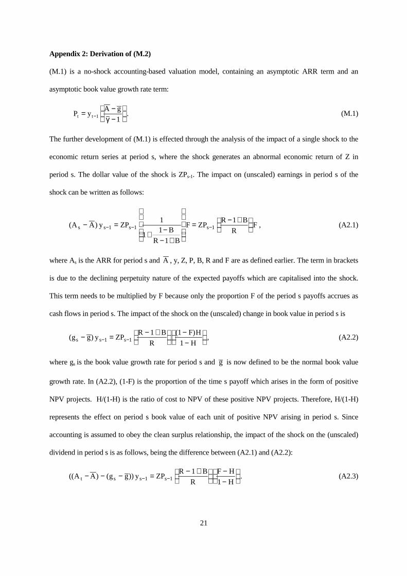
Appendix 2: Derivation of (M.2)

(M.1) is a no-shock accounting-based valuation model, containing an asymptotic ARR term and an

asymptotic book value growth rate term:

P yA g

t t= −−

−1 1γ

. (M.1)

The further development of (M.1) is effected through the analysis of the impact of a single shock to the

economic return series at period s, where the shock generates an abnormal economic return of Z in

period s. The dollar value of the shock is ZPs-1. The impact on (unscaled) earnings in period s of the

shock can be written as follows:

( ) ,A A y ZPB

R B

F ZPR B

RFs s s s− =

+ −− +

= − +

− − −1 1 1

1

11

1

1(A2.1)

where As is the ARR for period s and A , y, Z, P, B, R and F are as defined earlier. The term in brackets

is due to the declining perpetuity nature of the expected payoffs which are capitalised into the shock.

This term needs to be multiplied by F because only the proportion F of the period s payoffs accrues as

cash flows in period s. The impact of the shock on the (unscaled) change in book value in period s is

( )( )

,g g y ZPR B

R

F H

Hs s s− = − +

−−

− −1 1

1 1

1(A2.2)

where gs is the book value growth rate for period s and g is now defined to be the normal book value

growth rate. In (A2.2), (1-F) is the proportion of the time s payoff which arises in the form of positive

NPV projects. H/(1-H) is the ratio of cost to NPV of these positive NPV projects. Therefore, H/(1-H)

represents the effect on period s book value of each unit of positive NPV arising in period s. Since

accounting is assumed to obey the clean surplus relationship, the impact of the shock on the (unscaled)

dividend in period s is as follows, being the difference between (A2.1) and (A2.2):

(( ) ( )) .A A g g y ZPR B

R

F H

Ht s s s− − − = − +

−−

− −1 1

1

1(A2.3)

22

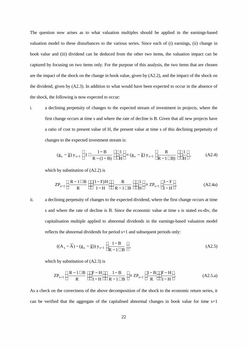
The question now arises as to what valuation multiples should be applied in the earnings-based

valuation model to these disturbances to the various series. Since each of (i) earnings, (ii) change in

book value and (iii) dividend can be deduced from the other two items, the valuation impact can be

captured by focusing on two items only. For the purpose of this analysis, the two items that are chosen

are the impact of the shock on the change in book value, given by (A2.2), and the impact of the shock on

the dividend, given by (A2.3). In addition to what would have been expected to occur in the absence of

the shock, the following is now expected to occur:

i. a declining perpetuity of changes to the expected stream of investment in projects, where the

first change occurs at time s and where the rate of decline is B. Given that all new projects have

a ratio of cost to present value of H, the present value at time s of this declining perpetuity of

changes to the expected investment stream is:

( )( )

( ))

,g g yB

R B Hg g y

R

R B Hs s s s− +−

− −

= −− +

− −1 11

1

1

1

1

1(A2.4)

which by substitution of (A2.2) is

ZPR B

R

F H

H

R

R B HZP

F

Hs s− −− +

−−

− +

= −−

1 1

1 1

1 1

1 1

1

( ). (A2.4a)

ii. a declining perpetuity of changes to the expected dividend, where the first change occurs at time

s and where the rate of decline is B. Since the economic value at time s is stated ex-div, the

capitalisation multiple applied to abnormal dividends in the earnings-based valuation model

reflects the abnormal dividends for period s+1 and subsequent periods only:

(( ) ( )) ,A A g g yB

R Bs s s− − − −− +

−1

1

1(A2.5)

which by substitution of (A2.3) is

ZPR B

R

F H

H

B

R BZP

B

R

F H

Hs s− −− +

−−

−− +

= −

−−

1 1

1

1

1

1

1

1. (A2.5.a)

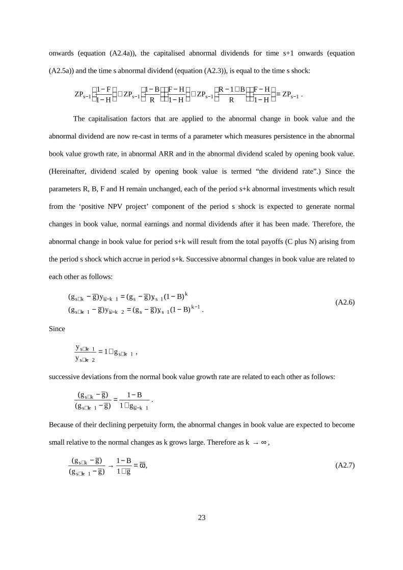
As a check on the correctness of the above decomposition of the shock to the economic return series, it

can be verified that the aggregate of the capitalised abnormal changes in book value for time s+1

23

onwards (equation (A2.4a)), the capitalised abnormal dividends for time s+1 onwards (equation

(A2.5a)) and the time s abnormal dividend (equation (A2.3)), is equal to the time s shock:

ZPF

HZP

B

R

F H

HZP

R B

R

F H

HZPs s s s− − − −

−−

+ −

−−

+ − +

−−

=1 1 1 11

1

1

1

1

1.

The capitalisation factors that are applied to the abnormal change in book value and the

abnormal dividend are now re-cast in terms of a parameter which measures persistence in the abnormal

book value growth rate, in abnormal ARR and in the abnormal dividend scaled by opening book value.

(Hereinafter, dividend scaled by opening book value is termed “the dividend rate”.) Since the

parameters R, B, F and H remain unchanged, each of the period s+k abnormal investments which result

from the ‘positive NPV project’ component of the period s shock is expected to generate normal

changes in book value, normal earnings and normal dividends after it has been made. Therefore, the

abnormal change in book value for period s+k will result from the total payoffs (C plus N) arising from

the period s shock which accrue in period s+k. Successive abnormal changes in book value are related to

each other as follows:

( ) ( ) ( )

( ) ( ) ( ) .

g g y g g y B

g g y g g y B

s k s k s sk

s k s k s sk

+ + − −

+ − + − −−

− = − −

− = − −1 1

1 2 11

1

1(A2.6)

Since

y

ygs k

s ks k

+ −

+ −+ −= +1

211 ,

successive deviations from the normal book value growth rate are related to each other as follows:

( )

( ).

g g

g g

B

gs k

s k s k

+

+ − + −

−−

= −+1 1

1

1

Because of their declining perpetuity form, the abnormal changes in book value are expected to become

small relative to the normal changes as k grows large. Therefore as k → ∞ ,

( )

( ),

g g

g g

B

gs k

s k

+

+ −

−−

→ −+

=1

1

1ω (A2.7)

24

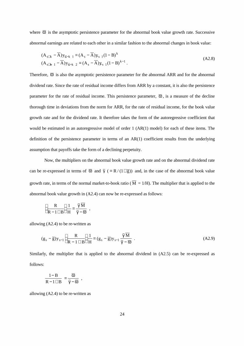
where ω is the asymptotic persistence parameter for the abnormal book value growth rate. Successive

abnormal earnings are related to each other in a similar fashion to the abnormal changes in book value:

( ) ( ) ( )

( ) ( ) ( ) .

A A y A A y B

A A y A A y B

s k s k s sk

s k s k s sk

+ + − −

+ − + − −−

− = − −

− = − −1 1

1 2 11

1

1(A2.8)

Therefore, ω is also the asymptotic persistence parameter for the abnormal ARR and for the abnormal

dividend rate. Since the rate of residual income differs from ARR by a constant, it is also the persistence

parameter for the rate of residual income. This persistence parameter, ω , is a measure of the decline

thorough time in deviations from the norm for ARR, for the rate of residual income, for the book value

growth rate and for the dividend rate. It therefore takes the form of the autoregressive coefficient that

would be estimated in an autoregressive model of order 1 (AR(1) model) for each of these items. The

definition of the persistence parameter in terms of an AR(1) coefficient results from the underlying

assumption that payoffs take the form of a declining perpetuity.

Now, the multipliers on the abnormal book value growth rate and on the abnormal dividend rate

can be re-expressed in terms of ω and γ ( / ( ))= +R g1 and, in the case of the abnormal book value

growth rate, in terms of the normal market-to-book ratio ( M = 1/H). The multiplier that is applied to the

abnormal book value growth in (A2.4) can now be re-expressed as follows:

R

R B H

M

− +

=−1

1 γγ ω

,

allowing (A2.4) to be re-written as

( ) ( ) .g g yR

R B Hg g y

Ms s s s−

− +

= −−− −1 11

1 γγ ω

(A2.9)

Similarly, the multiplier that is applied to the abnormal dividend in (A2.5) can be re-expressed as

follows:

1

1

−− +

=−

B

R B

ωγ ω

,

allowing (A2.4) to be re-written as

25

(( ) ( ))

(( ) ( )) .

A A g g yB

R B

A A g g y

s s s

s s s

− − − −− +

= − − −−

−

−

1

1

1

1

ωγ ω

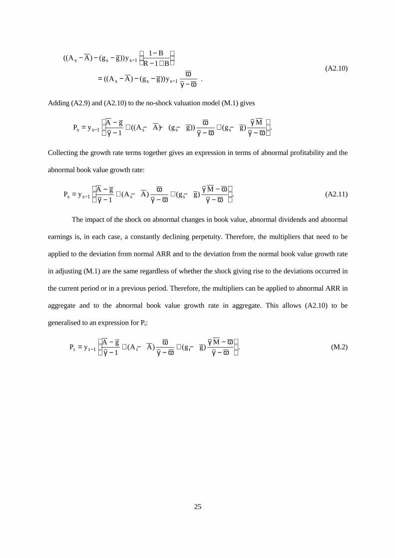
(A2.10)

Adding (A2.9) and (A2.10) to the no-shock valuation model (M.1) gives

P yA g

A A g g g gM

s s s s s=−−

+ − − −−

+ −−

−1 1γ

ωγ ω

γγ ω

(( ) ( )) ( ) .

Collecting the growth rate terms together gives an expression in terms of abnormal profitability and the

abnormal book value growth rate:

P yA g

A A g gM

s s s s=−−

+ −−

+ −−

−

−1 1γ

ωγ ω

γ ωγ ω

( ) ( ) . (A2.11)

The impact of the shock on abnormal changes in book value, abnormal dividends and abnormal

earnings is, in each case, a constantly declining perpetuity. Therefore, the multipliers that need to be

applied to the deviation from normal ARR and to the deviation from the normal book value growth rate

in adjusting (M.1) are the same regardless of whether the shock giving rise to the deviations occurred in

the current period or in a previous period. Therefore, the multipliers can be applied to abnormal ARR in

aggregate and to the abnormal book value growth rate in aggregate. This allows (A2.10) to be

generalised to an expression for Pt:

P yA g

A A g gM

t t t t=−−

+ −−

+ −−

−

−1 1γ

ωγ ω

γ ωγ ω

( ) ( ) . (M.2)

26

References

Bernard, V. (1993). ‘Accounting-based valuation methods, determinants of market-to-book ratios, and

implications for financial statements analysis’, Working paper, University of Michigan.

Copeland, T., T. Koller and J. Murrin (1995). Valuation: Measuring and Managing the Value of

Companies, Wiley.

Dixit, A and R. Pindyck. (1994). Investment under Uncertainty, Princeton.

Edey, H. (1962). ‘Business valuation, goodwill and the super-profit method’, in Baxter, W. and S.

Davidson (eds.), Studies in Accounting Theory, Sweet and Maxwell.

Edwards, E. and P. Bell (1961). The Theory and Measurement of Business Income, University of

California Press.

Feltham, G. and J. Ohlson (1995). ‘Valuation and clean surplus accounting for operating and financial

activities’, Contemporary Accounting Research 11: 689-731.

Feltham, G. and J. Ohlson (1996). ‘Uncertainty resolution and the theory of depreciation measurement’,

Journal of Accounting Research 34: 209-234.

McTaggart, J., P. Kontes and M. Mankins (1994). The Value Imperative, Free Press.

O’Hanlon, J. (1996). ‘The time-series properties of the components of clean surplus earnings: UK

evidence’, Journal of Business Finance and Accounting 23: 159-183.

Ohlson, J. (1995). ‘Earnings, book values and dividends in security valuation’, Contemporary

Accounting Research 11: 661-687.

Ou, J. and S. Penman (1993). ‘Financial statement analysis and the evaluation of market-to-book

ratios’, Working paper, Santa Clara University and University of California at Berkeley.

Peasnell, K. (1982). ‘Some formal connections between economic values and yields and accounting

numbers’ Journal of Business Finance and Accounting 9: 361-381.

Rappaport, A. (1986). Creating Shareholder Value: The New Standard for Business Performance, Free

Press.

27

Stern, J, G. Stewart and D. Chew (1995). ‘The EVA® financial management system’, Journal of Applied

Corporate Finance 8: 32-46.

Trigeorgis, L. (1996). Real Options, MIT Press.

28

Table 1: Numerical example of movement in economic value and in accounting book value in the setting described in Section 2 (for B=1).

Panel A: Movement in economic value:Period Opening

economicvalue

Payoff

Investment in new projects

Dividend Closingeconomic

value

Economic rate ofreturn (%)

Total Cash NPV ofPositive NPV

projects

Cash cost NPV Presentvalue

Notation foritem:

Pt-1 Ct+Nt Ct Nt It Nt It + Nt dt Pt (R-1)

Compositionof item:

= Pt-1

*1.20= (Ct+Nt)

* 0.70= (Ct+Nt)*(1-0.70)

= (Nt*0.667)/(1-0.667))

= (Ct+Nt)*(1-0.70)

= It + Nt =Ct - It = It + Nt = (Pt+dt-Pt-1)/Pt-1

1 100.00 120.00 84.00 36.00 72.00 36.00 108.00 12.00 108.00 20%2 108.00 129.60 90.72 38.88 77.76 38.88 116.64 12.96 116.64 20%3 116.64 139.97 97.98 41.99 83.98 41.99 125.97 14.00 125.97 20%

Panel B: Movement in accounting book value:Period Opening

book valueCash payoff Depreciation Accounting

earningsDividend Closing

book valueAccounting

rate ofreturn (%)

Residualincome

Rate ofresidual

income (%)Notation foritem:

yt-1 Ct -yt-1B xt dt yt At xat χt

a

Compositionof item:

= (Ct + Nt)* 0.70

-yt-1 = Ct - yt-1B = Ct - It = yt-1 + xt - dt = xt/yt-1 = xt

- (yt-1*0.20)= xa

t / yt-1

1 100.00 84.00 -100.00 -16.00 12.00 72.00 -16% -36.00 -36%2 72.00 90.72 -72.00 18.72 12.96 77.76 26% 4.32 6%3 77.76 97.98 -77.76 20.22 14.00 83.98 26% 4.67 6%

Continued on next page...

29

Continued from previous page...

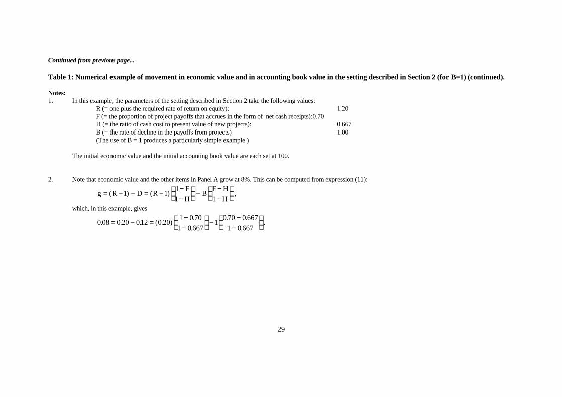
Table 1: Numerical example of movement in economic value and in accounting book value in the setting described in Section 2 (for B=1) (continued).

Notes:1. In this example, the parameters of the setting described in Section 2 take the following values:

R (= one plus the required rate of return on equity): 1.20F (= the proportion of project payoffs that accrues in the form of net cash receipts):0.70H (= the ratio of cash cost to present value of new projects): 0.667B (= the rate of decline in the payoffs from projects) 1.00(The use of B = 1 produces a particularly simple example.)

The initial economic value and the initial accounting book value are each set at 100.

2. Note that economic value and the other items in Panel A grow at 8%. This can be computed from expression (11):

g R D RF

HB

F H

H= − − = − −

−

− −−

( ) ( ) ,1 11

1 1which, in this example, gives

0 08 0 20 012 0 201 0 70

1 0 6671

0 70 0 667

1 0 667. . . ( . )

.

.

. .

..= − = −

−

− −−