An Efficient and Exact Subdivision Algorithm

for Isolating Complex Roots of a Polynomial

and its Complexity Analysis

Michael Sagraloff

Max Planck Institute for Informatics, Saarbrucken

Chee K. Yap

Courant Institute, NYU, New York

Abstract

We introduce an exact subdivision algorithm CEVAL for isolating complex roots ofa square-free polynomial. The subdivision predicates are based on evaluating theoriginal polynomial or its derivatives, and hence is easy to implement. It can be seenas a generalization of a previous real root isolation algorithm called EVAL. Undersuitable conditions, the algorithm is applicable for general analytic functions.

We provide a complexity analysis of our algorithm on the benchmark problemof isolating all complex roots of a square-free polynomial with Gaussian integercoefficients. The analysis is based on a novel technique called δ-clusters. This anal-ysis shows, somewhat surprisingly, that the simple EVAL algorithm matches (upto logarithmic factors) the bit complexity bounds of current practical exact algo-rithms such as those based on Descartes, Continued Fraction or Sturm methods.Furthermore, the more general CEVAL also achieves the same complexity.

Key words: root isolation, subdivision methods, complex roots, Bolzano method

1 Introduction

Root finding might be called the Fundamental Problem of Algebra, after theFundamental Theorem of Algebra [39,41,44]. The literature on root finding isextremely rich, with a large classical literature. The work of Schonhage [39]

Email addresses: msagralo@mpi-inf.mpg.de (Michael Sagraloff),yap@cs.nyu.edu (Chee K. Yap).

Preprint submitted to Elsevier 30 October 2009

marks the beginning of complexity-theoretic approaches to the FundamentalProblem. Pan [33] provides a history of root-finding from the complexity viewpoint; see McNamee [22] for a general bibliography. The root finding problemcan be studied as two distinct problems: root isolation and root refinement. Inthe complexity literature, the main focus is on what we call the benchmark

problem, that is, isolating all the complex roots of a polynomial f of degree nwith integer coefficients of at most L bits. Let T (n, L) denote the (worst case)bit complexity of this problem. There are three variations on this benchmarkproblem:

• We can ask for only the real roots. Special techniques apply in this importantcase [7,16]. E.g., Sturm [20,37,9], Descartes [5,38,27,12,10], and continuedfraction methods [1,40].• We can seek the arithmetic complexity of this problem, that is, we seek to

optimize the number TA(n, L) of arithmetic operations.• We can add another parameter p > 0, and instead of isolation, we may seek

to approximate each of the roots to p relative or absolute bits.

Schonhage achieved a bound of T (n, L) = O(n3L) for the benchmark iso-lation problem where O indicates the omission of logarithmic factors. Thisbound has essentially remained intact. Pan and others [33,29] have giventheoretical improvements in the sense of achieving TA(n, L) = O(n2L) andT (n, L) = TA(n, L) · O(n), thus achieving record bounds in both bit com-plexity and arithmetic complexity. Theoretical algorithms designed to achieverecord bounds for the benchmark problem have so far not been used in prac-tice. Moreover, the benchmark problem is inappropriate for some applications.For instance, we may only be interested in the first positive root (as in rayshooting in computer graphics), or the roots in some limited neighborhood.In the numerical literature, there are many algorithms that are widely usedand effective in practice but lack a guarantee on the global behavior (cf. [33]for discussion). Some “global methods” such as the Weierstrass or Durant-Kerner method that simultaneously approximates all roots seem ideal for thebenchmark problem and work well in practice, but their convergence and/orcomplexity analysis are open. Thus, the benchmark complexity, despite its the-oretical usefulness, has limitation as sole criterion in evaluating the usefulnessof root isolation algorithms.

There are two sources of literature on “practical” root isolation algorithms: (1)One is the exact computation literature, providing algorithms used in variousalgebraic applications and computer algebra systems. Such exact algorithmshave a well-developed complexity analysis and there is considerable computa-tional experience especially in the context of cylindrical algebraic decompo-sition. The favored root isolation algorithms here, applied to the benchmarkproblem, tend to lag behind the theoretical algorithms by a factor of nL. Nev-ertheless, current experimental data justify their use [38,16]. (2) The other

2

is the numerical literature, mentioned above. Although numerical algorithmstraditionally lack any exactness guarantees, they have many advantages thatpractitioners intuitively understand: compared to algebraic methods, they areeasier to implement and their complexity is more adaptive. Hence, there isa growing interest to constructing numerical algorithms that are exact andefficient. This paper is a contribution along this line.

1.1 The Subdivision Approach

Among the practical exact root isolation algorithms, the subdivision paradigmis perhaps the most widely used. This paradigm is a generalization of binarysearch in which we begin with a domain (say a box B0 ⊆ C) and recursivelysubdivide the boxes to search for roots. Unlike the theoretical algorithms orglobal methods above, subdivision algorithms have a strong advantage of be-ing “local” as they can restrict computational effort only to the given initialbox B0, in order to find roots near B0. If there are few or no roots in B0,such methods can terminate quickly. The “subdivision” terminology derivesfrom the use of such algorithms in meshing curves and surfaces [21]; root iso-lation is just meshing in 1-D. The principle action of subdivision algorithmsis the subdivision phase that operates on a queue Q containing subboxesof B0. Initially, Q = {B0}. In each iteration, a box B is removed from Q andtested with an exclusion predicate Cout and an inclusion predicate Cin.If Cout(B) holds, B is discarded; if Cin(B) holds, then B is output. Otherwise,we subdivide B into four children boxes and put them back into Q. For rootisolation, Cout(B) guarantees that B has no zeros, and Cin(B) guarantees thatthere is a unique zero in B. For real roots, we would use intervals instead ofboxes. The general structure of many subdivision algorithms is fairly simple;in [21], the “generic subdivision algorithm” is viewed as a sequence of fourphases: boundary, subdivision (described above), refinement, and construc-tion. For our root isolation problem, we can omit the boundary and refinementphases. The construction phase amounts to ensuring that the output boxes arepairwise disjoint. Since finding a root is metaphorically like “finding a needlein a hay stack”, an efficient exclusion predicate Cout is crucial to the successof such algorithms. Here, numerical forms of Cout such as those used in thispaper are relatively cheap and have advantages over algebraic ones.

1.2 Three Principles for Subdivision

We compare three general principles used in subdivision algorithms for realroot isolation: theory of Sturm sequences, Descartes’ rule of sign, and theBolzano principle. These principles are used in the exclusion and inclusionpredicates of the corresponding algorithms. Continued Fraction Solvers can beviewed as extended Descartes methods since they use Descartes’ Rule of Sign

3

as their main predicates, but combine it with an exclusion predicate based ona root bound. Although the Continued Fraction method has not been provento achieve better worse case complexity [40,23,13], a significant speed up canbe observed in practice [13,1,15]. This paper concentrates on the Bolzanoprinciple, also known as the Bolzano theorem. It is simple and intuitive: if acontinuous real function f(x) satisfies f(a)f(b) < 0 then there is a point cbetween a and b such that f(c) = 0. Furthermore, if f is differentiable and f ′

does not vanish on (a, b) then this root is unique in (a, b). In recent years, algo-rithms based on the first two principles have been called (respectively) Sturmmethod [37,20,9] and the Descartes method 1 [5,12,19,6]. By analogy, we maycall algorithms based on the Bolzano principle the Bolzano method [25,4,3].Note that the Bolzano principle is an analytic one, while Sturm and Descartesare more algebraic. The complexity analysis of Bolzano methods seems to benew, prompted in part by interest in exact numerical methods in meshing alge-braic surfaces [35,21,2]. Perhaps it is no surprise that Bolzano methods couldoutperform the more sophisticated algebraic methods in practice. Somewhatsurprisingly, the results of this paper indicate that Bolzano methods could alsomatch the theoretical complexity of algebraic methods as well.

There are two basic complexity measures for subdivision algorithms: the sub-division tree size S(n, L) and the bit complexity P (n, L) of the subdivisionpredicates. Thus, T (n, L) ≤ S(n, L)P (n, L). But the analysis in this papershows that T (n, L) may be smaller than S(n, L)P (n, L) by a factor of n. Treesize in the Sturm method is optimal in a very strong sense: for any polyno-mial f(x) and for any interval I0, the Sturm subdivision tree is minimum inan absolute, not asymptotic, sense. For the benchmark problem where f(x)has degree n and L-bit integer coefficients, this tree size was shown to beO(n(L + log n)) by Davenport [8] in 1985. This is optimal if L ≥ log n [12].Modern algorithmic treatment of the Descartes method began with Collins andAkritas [5]. The tree size in the Descartes method was only recently provento be O(n(L + log n)) [12]. In this paper, we will prove that the tree size inthe Bolzano method is O(n(L + log n)) for real roots. Furthermore, for ourextension of the Bolzano method for complex roots the corresponding tree sizeis O(n2(L + log n)). Despite this larger tree size, we prove that both real andcomplex Bolzano have O(n4L2) bit complexity, matching Descartes and Sturm.

Johnson [16] has shown empirically that the Descartes method is more efficientthan Sturm. Rouillier and Zimmermann [38] implemented a highly efficient ex-act real root isolation algorithm based on the Descartes method. Since theirtheoretical complexity bounds are indistinguishable, any practical advantageof Descartes over Sturm must be derived from the fact that the predicatesin the Descartes method are cheaper. We believe that the Bolzano method

1 Note that we avoid the possessive “Descartes method” as Descartes did not en-vision such algorithms.

4

has a similar advantage over Descartes. This has not yet been demonstrated.Nevertheless, it has an advantage of a different kind: The Bolzano method isapplicable to a much wider class of functions — most common analytic func-tions are amenable. Furthermore, this paper shows that the Bolzano methodcan be extended to the domain of complex numbers.

1.3 Contributions of this paper

1. Our root isolation algorithm is a contribution to a growing list of exact al-gorithms based on numerical (as opposed to algebraic) techniques and simplesubdivision. Numerical subdivision methods are widely used in practice, beingeasy to implement and having adaptive complexity. In comparison to existingexact practical methods for real root isolation (Descartes, Sturm, ContinuedFraction) it extends to most common analytic functions and also to the do-main of complex numbers.

2. This paper represents one of the first complexity analysis of exact numericalsubdivision methods based on the Bolzano principle. It uses a novel techniqueof δ-clusters, from which we expect other application as well. Surprisingly, ouranalysis shows that the simple Bolzano principle already yields an algorithmEVAL whose worst-case bit-complexity matches those of more sophisticatedmethods like Sturm or Descartes. Also unexpected is that the complex ana-logue CEVAL achieve the same bit complexity as EVAL (despite the fact thatin terms of tree size, that of CEVAL is quadratic in the real size).

1.4 Overview of Paper

Section 2 reviews related work. The algorithm is presented in Section 3.Therein we also summarize the results of our complexity analysis accomplishedin Section 5 by the use of the new concept of δ−clusters. Section 4 developsbasic tools for proving the correctness of the algorithm. Section 6 addressesissues in implementing our algorithm exactly. We conclude in Section 7.

2 Prior Work

The main distinction among the various subdivision algorithms is the choice 2

of tests or predicates. One approach is based on doing root isolation on theboundary of the boxes. Pinkert [34] and Wilf [43] (see also [44]) use Sturm-likesequences, while Collins and Krandick [18] considered Descartes method. Suchapproaches are related to topological degree methods [28], which go back toBrouwer (1924).

2 We shall use the terms “predicate” and “test” interchangeably.

5

2.1 Weyl’s Approach

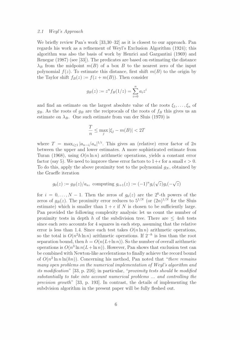
We briefly review Pan’s work [33,30–32] as it is closest to our approach. Panregards his work as a refinement of Weyl’s Exclusion Algorithm (1924); thisalgorithm was also the basis of work by Henrici and Gargantini (1969) andRenegar (1987) (see [33]). The predicates are based on estimating the distanceλB from the midpoint m(B) of a box B to the nearest zero of the inputpolynomial f(z). To estimate this distance, first shift m(B) to the origin bythe Taylor shift fB(z) := f(z +m(B)). Then consider

gB(z) := znfB(1/z) =n∑

i=0

aizi

and find an estimate on the largest absolute value of the roots ξ1, . . . , ξn ofgB. As the roots of gB are the reciprocals of the roots of fB this gives us anestimate on λB. One such estimate from van der Sluis (1970) is

T

n≤ max

j|ξj −m(B)| < 2T

where T = maxi≥1 |an−i/an|1/i. This gives an (relative) error factor of 2nbetween the upper and lower estimates. A more sophisticated estimate fromTuran (1968), using O(n lnn) arithmetic operations, yields a constant errorfactor (say 5). We need to improve these error factors to 1+ǫ for a small ǫ > 0.To do this, apply the above proximity test to the polynomial gN , obtained bythe Graeffe iteration

g0(z) := gB(z)/an, computing gi+1(z) := (−1)ngi(√z)gi(−

√z)

for i = 0, . . . , N − 1. Then the zeros of gk(z) are the 2k-th powers of thezeros of gB(z). The proximity error reduces to 51/N (or (2n)1/N for the Sluisestimate) which is smaller than 1 + ǫ if N is chosen to be sufficiently large.Pan provided the following complexity analysis: let us count the number ofproximity tests in depth h of the subdivision tree. There are ≤ 4nh testssince each zero accounts for 4 squares in each step, assuming that the relativeerror is less than 1.4. Since each test takes O(n lnn) arithmetic operations,so the total is O(n2h lnn) arithmetic operations. If 2−h is less than the rootseparation bound, then h = O(n(L+lnn)). So the number of overall arithmeticoperations is O(n3 lnn(L+lnn)). However, Pan shows that exclusion test canbe combined with Newton-like accelerations to finally achieve the record boundof O(n2 lnn ln(hn)). Concerning his method, Pan noted that “there remainsmany open problems on the numerical implementation of Weyl’s algorithm andits modification” [33, p. 216]; in particular, “proximity tests should be modifiedsubstantially to take into account numerical problems ... and controlling theprecision growth” [33, p. 193]. In contrast, the details of implementing thesubdvision algorithm in the present paper will be fully fleshed out.

6

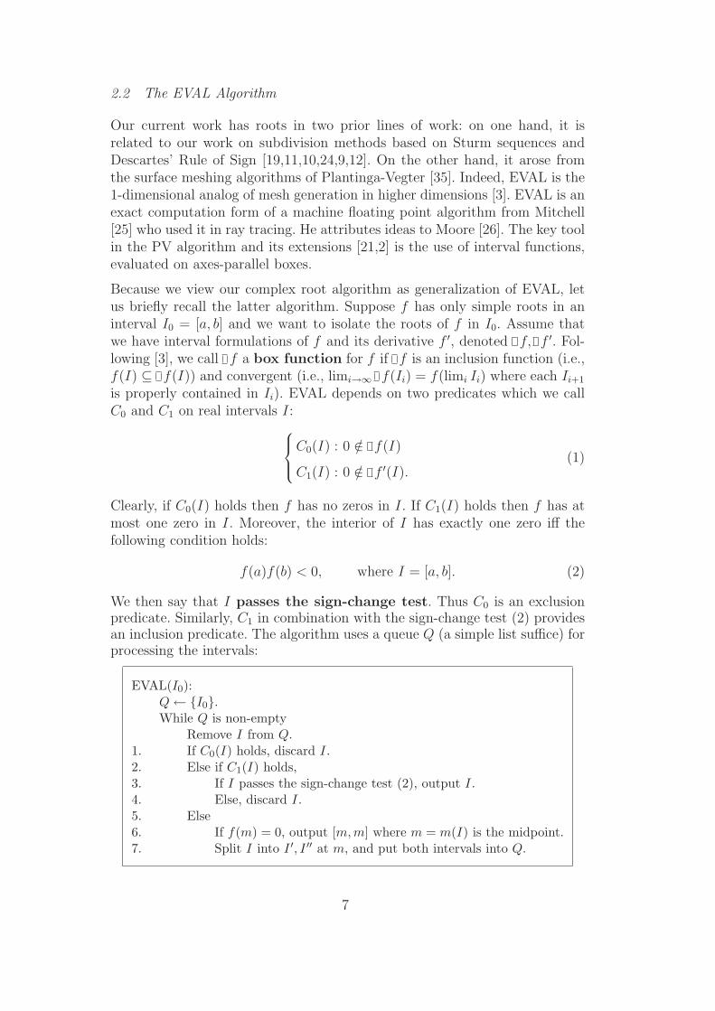
2.2 The EVAL Algorithm

Our current work has roots in two prior lines of work: on one hand, it isrelated to our work on subdivision methods based on Sturm sequences andDescartes’ Rule of Sign [19,11,10,24,9,12]. On the other hand, it arose fromthe surface meshing algorithms of Plantinga-Vegter [35]. Indeed, EVAL is the1-dimensional analog of mesh generation in higher dimensions [3]. EVAL is anexact computation form of a machine floating point algorithm from Mitchell[25] who used it in ray tracing. He attributes ideas to Moore [26]. The key toolin the PV algorithm and its extensions [21,2] is the use of interval functions,evaluated on axes-parallel boxes.

Because we view our complex root algorithm as generalization of EVAL, letus briefly recall the latter algorithm. Suppose f has only simple roots in aninterval I0 = [a, b] and we want to isolate the roots of f in I0. Assume thatwe have interval formulations of f and its derivative f ′, denoted f, f ′. Fol-lowing [3], we call f a box function for f if f is an inclusion function (i.e.,f(I) ⊆ f(I)) and convergent (i.e., limi→∞ f(Ii) = f(limi Ii) where each Ii+1

is properly contained in Ii). EVAL depends on two predicates which we callC0 and C1 on real intervals I:

C0(I) : 0 /∈ f(I)

C1(I) : 0 /∈ f ′(I).(1)

Clearly, if C0(I) holds then f has no zeros in I. If C1(I) holds then f has atmost one zero in I. Moreover, the interior of I has exactly one zero iff thefollowing condition holds:

f(a)f(b) < 0, where I = [a, b]. (2)

We then say that I passes the sign-change test. Thus C0 is an exclusionpredicate. Similarly, C1 in combination with the sign-change test (2) providesan inclusion predicate. The algorithm uses a queue Q (a simple list suffice) forprocessing the intervals:

EVAL(I0):Q← {I0}.While Q is non-empty

Remove I from Q.1. If C0(I) holds, discard I.2. Else if C1(I) holds,3. If I passes the sign-change test (2), output I.4. Else, discard I.5. Else6. If f(m) = 0, output [m, m] where m = m(I) is the midpoint.7. Split I into I ′, I ′′ at m, and put both intervals into Q.

7

Termination and correctness are easy to see. The output intervals either havethe exact form [m,m] or are regarded as open intervals (a, b). This algorithmis easy to implement exactly if we assume that all intervals are represented bydyadic numbers, and f, f ′ are computable functions on dyadic intervals, andthe sign of f on dyadic numbers are computable. Obviously, this algorithm isan analytic one – we can use it to find simple roots of most common analyticfunctions f .

In this paper, the predicates (1) are assumed to be implemented as

C0(I) : |f(m)| > ∑k≥1

|f (k)(m)|k!

(w(I)

2

)k,

C1(I) : |f ′(m)| > ∑k≥2

|f (k)(m)|(k−1)!

(w(I)

2

)k−1.

(3)

where m = (a+b)/2 and w(I) = (b−a). This is closely related to the centeredform used in [3,36].

3 A New Complex Root Algorithm and its Complexity

In this section, we will state our main results in three parts. We will (1)describe our main algorithm called CEVAL, (2) prove its correctness, and (3)state bounds on its complexity. Details of the correctness proof and complexitybounds are deferred to Sections 4 and 5 respectively.

Throughout this paper, we fix a square-free polynomial f ∈ C[z]. We alsowrite it as f(z) = f(x+ iy) = u(x, y)+ iv(x, y) where i =

√−1, x = Re(z) and

y = Im(z) are real and imaginary parts of z, and u, v : R2 → R. If z′ = x′ + iy′

then we write 〈z, z′〉 = xx′ + yy′. Absolute value is denoted |z| :=√〈z, z〉.

Sometimes, instead of viewing u(x, y) as a function of two real variables, weview u as a real-valued complex function, writing u(z) = u(x+ iy) for u(x, y).Similar remarks hold for v(x, y). Let S1 = [0, 2π) denote the set of angles inradians. Then arg(ξ) ∈ S1 denotes the argument of a complex number ξ ∈ C.If (x, y) ∈ R

2, we also write arg(x, y) for arg(x+ iy).

3.1 Complex Geometry

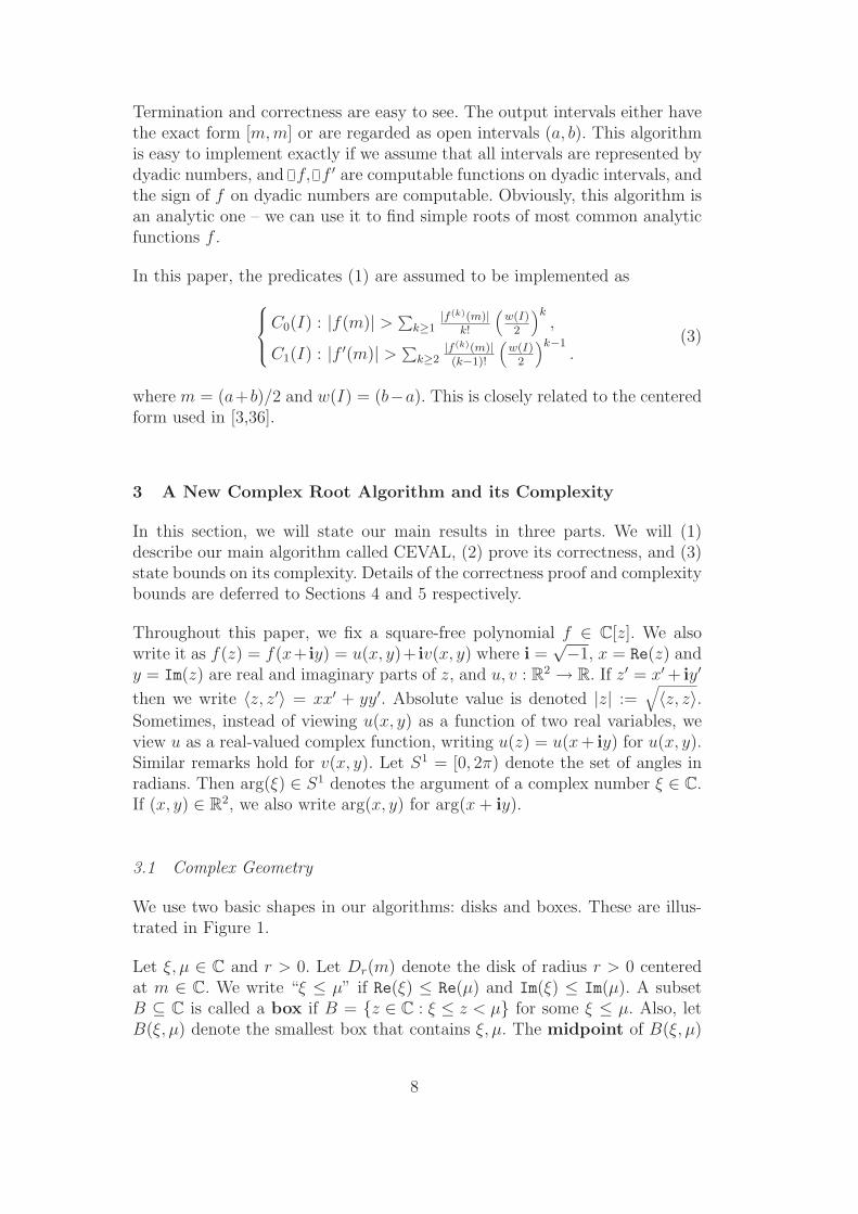
We use two basic shapes in our algorithms: disks and boxes. These are illus-trated in Figure 1.

Let ξ, µ ∈ C and r > 0. Let Dr(m) denote the disk of radius r > 0 centeredat m ∈ C. We write “ξ ≤ µ” if Re(ξ) ≤ Re(µ) and Im(ξ) ≤ Im(µ). A subsetB ⊆ C is called a box if B = {z ∈ C : ξ ≤ z < µ} for some ξ ≤ µ. Also, letB(ξ, µ) denote the smallest box that contains ξ, µ. The midpoint of B(ξ, µ)

8

Disk Dr(m) Box B = B(µ, ξ)

µ

ξ

r

m

r(B)

w(B

)

d(B)

m(B)

Fig. 1. Two geometric shapes in the complex plane: disk and box

is m(B) := (ξ + µ)/2. If ξ < µ, then the width, diameter, and radius ofB(ξ, µ) are (respectively) given by:

w(B) := min {Re(µ)− Re(ξ), Im(µ)− Im(ξ)}d(B) := max {Re(µ)− Re(ξ), Im(µ)− Im(ξ)} ,r(B) :=

1

2

√w(B)2 + d(B)2.

We can split a box B into four equally dimensioned subboxes, called thechildren of B. The boundary of a region R ⊆ C is denoted ∂R (R is usuallya disk or a box). A box B or disk D is said to be isolating if it containsexactly one zero of f(z). Our goal is to find isolating disks for each of thecomplex zeros of f(z) in a given box B0 ⊆ C.

3.2 Complex Analogues of the C0 and C1 Predicates

The EVAL algorithm in 2.2 is based on the interval predicates, C0 and C1 in(1). We now provide the complex analogues of these predicates; disks will nowplay the role of intervals. For m ∈ C and K, r > 0, define the test T fK :

T fK(m, r) : |f(m)| > K∑

k≥1

∣∣∣∣∣f (k)(m)

k!

∣∣∣∣∣ rk. (4)

Since f is fixed in this paper, we simply write TK(m, r) for T fK(m, r). Also,

when f ′ is used in place of f , we may write T ′K(m, r) for T f

′

K (m, r). Moreover,for any disk D, we may also write TK(D) for TK(m(D), r(D)), etc. Our firstlemma shows that these tests (for suitable K) provide the analogues of the C0

and C1 predicates in (1):

Lemma 1. Consider any disk D:

(i) If T1(D) holds then D contains no zeros of f .

(ii) If T ′√2(D) holds, then D has at most one zero of f .

Thus, the test T1(D) serves as an exclusion predicate for the disk D. Part(i)

9

is obvious while Part(ii) is in Lemma 8 in Section 4.1.

3.3 The Eight Point Test

To extend the test T ′√2(D) in Lemma 1 into an inclusion predicate, we need

the analogue of the sign-change test (2). We now try to detect points wherethe curves u = 0 and v = 0 cross the boundary of D. Such points can beidentified with angles as follows.

Let φ, φ′, θ be angles. We say that there is a u-crossing of Dr(m) at φ if

u(m + reiφ) = 0. We also need crossings not to be too close together: say φand φ′ are θ-separated if θ ≤ |φ−φ′| ≤ 2π− θ. Note that this notion is non-vacuous only if θ ≤ π, and non-trivial only if θ ≥ 0. The notion of v-crossing

is similarly defined.

SW

W

NE

SE

S

E

N

NW

Dr(m)

D4r(m)

m

Fig. 2. 8 compass points on D4r.

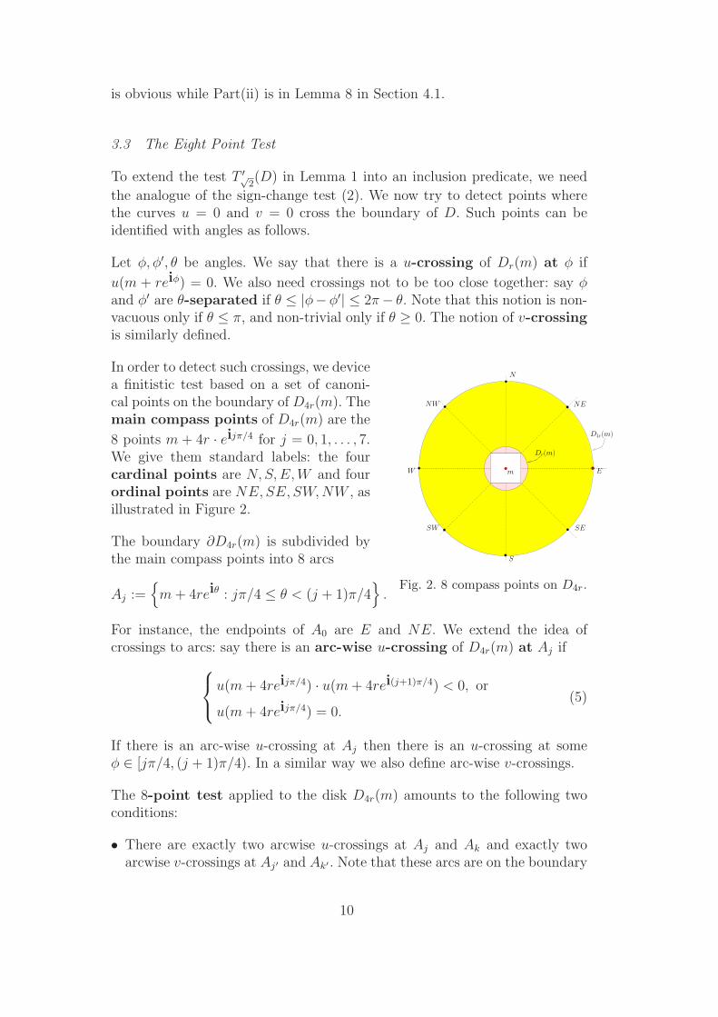
In order to detect such crossings, we devicea finitistic test based on a set of canoni-cal points on the boundary of D4r(m). Themain compass points of D4r(m) are the

8 points m + 4r · eijπ/4 for j = 0, 1, . . . , 7.We give them standard labels: the fourcardinal points are N,S,E,W and fourordinal points are NE,SE, SW,NW , asillustrated in Figure 2.

The boundary ∂D4r(m) is subdivided bythe main compass points into 8 arcs

Aj :={m+ 4reiθ : jπ/4 ≤ θ < (j + 1)π/4

}.

For instance, the endpoints of A0 are E and NE. We extend the idea ofcrossings to arcs: say there is an arc-wise u-crossing of D4r(m) at Aj if

u(m+ 4reijπ/4) · u(m+ 4rei(j+1)π/4) < 0, or

u(m+ 4reijπ/4) = 0.(5)

If there is an arc-wise u-crossing at Aj then there is an u-crossing at someφ ∈ [jπ/4, (j + 1)π/4). In a similar way we also define arc-wise v-crossings.

The 8-point test applied to the disk D4r(m) amounts to the following twoconditions:

• There are exactly two arcwise u-crossings at Aj and Ak and exactly twoarcwise v-crossings at Aj′ and Ak′ . Note that these arcs are on the boundary

10

of D4r(m), not Dr(m).

• These pairs of crossings are interleaving in the following sense: either j <j′ < k < k′ or j′ < j < k′ < k.

If any of these conditions does not hold, we say the disk fails the 8-point test.

Theorem 2 (Success of 8-Point Test). Suppose T ′6(m, 4r) holds and the 8-

point test is applied to D4r(m).

(i) If D4r(m) fails the 8-point test, then Dr(m) is not isolating.

(ii) If D4r(m) passes the 8-point test, then D4r(m) is an isolating disk.

We view Theorem 2 as providing a “weak” inclusion predicate for the diskDr(m) because, in case the predicate holds, we do not guarantee an isolatedroot in Dr(m), but only in D4r(m). Most of Section 3.6 is devoted to the proofof this theorem.

3.4 The Root Isolation Algorithm CEVAL

We present the complex analogue of EVAL, called CEVAL:

CEVAL(B0, f):Input: Box B0, and polynomial f(z) with only simple roots.Output: List L of pairwise disjoint isolating disks with centers in B0.

Q← {B0}. L ← ∅.While Q is non-empty

Remove B from Q. Let m = m(B) and r = r(B).1. If T1(m, r) holds, discard B.2. Else if T ′

6(m, 4r) and T ′√2(m, 8r) hold:

2.1 If D4r(m) fails the 8-point test, discard B.2.2 Else if D4r(m) intersects any disk D′ in L,

replace D′ by the smaller of D4r(m) and D′.2.3 Else insert D4r(m) into L.3. Else

Split B into four children and insert them into Q.

3.5 Remarks on CEVAL

Note that CEVAL is described within an algebraic RAM model of computa-tion. To implement CEVAL exactly, we need to attend to several details. Wemake some preliminary remarks here, deferring other details to Section 6.

11

(i) This description of CEVAL is close to what one can directly implementusing an arbitrary precision floating point package. Irrational operations (e.g.,in the definition of r(B) can easily be replaced by a dyadic approximation.E.g., Instead of TK(m, r(B)), you can use the predicate TK(m, δ(B)) whereδ(B) := 3

4w(B) > r(B) is a dyadic value. Furthermore, you may replace

K =√

2 by K = 3/2 and the ordinal compass points SE,NE,NW,SW =

m + w(B)(± 1

2√

2± 1

2√

2i)

by SE,NE,NW,SW = m + w(B)(±20

29± 21

29i),

respectively. The last replacement is justified by Theorem 14.

(ii) Note that in Step 2, we not only require T ′6(m, 4r), but also T ′√

2(m, 8r).

This is to ensure that whenever two discs in L overlap, we can discard eitherone of them according to Lemma 1 (in Step 2.2, we discard the larger one).

(iii) In Step 2.2, there is an implicit search of the list L for disks that intersectsD4r(m). For simplicity, we may assume a simple linear search. Since the sizeof L is non-decreasing, each search time is at most proportional to the outputsize of L, which is at most n.

(iv) The reader may also note that although an isolating diskD in L is centeredin B0, there is no guarantee that the isolated root z0 ∈ D actually belongsto B0. If we like, we could refine this algorithm with an additional parameterε > 0 and guarantee that z0 ∈ B0⊕Dε(0) (where ⊕ denotes Minkowski sum).This refinement does not seem necessary in practice.

3.6 Correctness Statement

This is comprised of three claims:

Theorem 3. (Correctness)

(a) The algorithm halts.

(b) Throughout the algorithm, L is a list of pairwise disjoint isolating disks.Each disk is centered at some point of B0.

(c) At termination, each zero of f(z) in B0 is isolated by some disk in L.

Claim (a) will be proven in a much stronger form when we give explicit com-plexity bounds later. However, it is instructive to see that, in general, haltingis guaranteed if f(z) has only simple roots in B0. If the algorithm does nothalt, then there is an infinite sequence (B0, B1, B2, . . .) of boxes where Bi+1

is a child of Bi, and each Bi fails the T1, T′6, and T ′√

2predicates. Thus the

sequence converges to a point z∗ = ∩iBi. By the convergence of these diskpredicates, this implies that f(z∗) = f ′(z∗) = 0, contradicting our assumptionthat f has simple roots in B0.

12

To see (b), observe that a disk D4r(m) is only inserted into L in Steps 2.2 or2.3. This happens after it passes the T ′

6-test, the 8-point test, and the T ′√2-test

on D8r(m). Lemma 1(ii) guarantees that such disks are isolating.

To see claim (c), we must show that no discarded box B ⊆ B0 contains a rootof f . Observe that boxes B ⊆ B0 are discarded in one of three steps of thealgorithm: Steps 1, 2.1, or 2.2. Step 1 is justified by Lemma 1(i) and Step 2.1is justified by Lemma 1(i). Finally, Step 2.2 is justified by remark (ii) in 3.5.

It is important to note that a disk in L might isolate a root of f that liesoutside B0.

3.7 Complexity Results

We now summarize the results of the complexity analysis of our algorithm;the actual proofs are found in Section 5. For this purpose, we consider thebenchmark problem of isolating all the roots of a square-free polynomial ofdegree n with coefficients that are L-bit Gaussian integers. In fact, there islittle complexity difference between Gaussian integers and ordinary rationalintegers. The initial start box may be assumed to be B0 = B(−2L(1+i), 2L(1+i)). According to Cauchy’s bound [44] B0 contains all the roots of f .

As noted, the efficiency of subdivision methods crucially depends on the choiceof the exclusion predicate. By simple modification, you can reformulate ouralgorithm by using any box function. You may apply a simple method suchHorner’s scheme applied to the initial polynomial f at each step. Althoughthis is relatively cheap, this approach may suffer from strong overestimationfor many boxes, in particular for those where the higher derivatives are smallin relation to those at the origin. This may result in a huge subdivision tree,rendering the overall algorithm useless. Our chosen predicates T fK are basedon the Taylor expansions at the centers of boxes, and thus they profit fromthe local information on the values of the higher order derivatives. We remarkthat this is common to other efficient methods for real root isolation – thereare implicit Taylor expansions in the Descartes method, for instance.

3.7.1 Cluster Analysis and Tree Size

Let us denote the subdivision trees, induced by CEVAL and EVAL by TCE

and TEV respectively. Before stating our results that bounds the sizes of TCE

and TEV , it is instructive to first give a crude estimate.

13

We start with a reformulation of the predicate T fK :

T fK(m, r) :∑

k≥1

∣∣∣∣f (k)(m)

f(m)

∣∣∣∣rk

k!<

1

K

It is easy to see (Section 5.2) that Σk(m) := (∑

i1

|m−zi|)k constitutes an upper

bound on λk := |f (k)(m)||f(m)| for all k ≥ 1, where z1, . . . , zn denote the complex

roots of f . Therefore, if Σ1(m) < ν for a ν > 0, then∑

k≥1

∣∣∣f(k)(m)f(m)

∣∣∣ rk

k!< eνr−1.

We easily verify that T fK(m, r) succeeds if (see also Lemma 21)

Σ1(m) =n∑

i=1

1

|m− zi|<

1

rln

(1 +

1

K

).

Now let us consider an arbitrary box B during the subdivision. If its midpointm(B) fulfills |m(B)− zi| > 2n · r(B) for all i = 1, . . . , n then T1(m(B), r(B))succeeds according to the above consideration, thus B is discarded. For eachroot zi, there exist at most O(n2) disjoint boxes B of the same size such that|m(B)−zi| ≤ 2n·r(B). Thus, in total, at most O(n3) boxes are retained. Fromthis straightforward observation we immediately derive the upper boundO(n3)on the width of TCE. This consideration is based on a pretty rough estimationof Σ1 which assumes that, from a given point m, the distances to all roots zihave roughly the same minimal value. In Section 5.1 we consider so called δ-clusters of roots which are related to the size δ of boxes at a certain subdivisionlevel. We show that outside some “smaller” neighborhood of the roots of fthe sum Σ1(m) is sufficiently small to guarantee the success of our exclusionpredicate T1 (see also Theorem 19):

Theorem 4. Let z1, . . . , zn be points in the complex space and δ > 0 an arbi-trary real value. Then there exist disjoint, axes-parallel, open boxesB1, . . . , Bk ⊂C, k ≤ n2, with the following properties:

(i) The union B :=⋃i=1,...,k Bi of all boxes covers all points z1, . . . , zn.

(ii) B covers an area of less than or equal to 4n2δ2.

(iii) For each point p /∈ B we have∑n

i=11

|p−zi| ≤2(1+ln⌈n/2⌉)

δ.

From this result it follows directly that the width of TCE is O((n lnn)2) (The-orem 22). In case of the EVAL algorithm it turns out that the width of TEV

can be bounded by O(n lnn) (Theorem 23). A more refined argument in theproof of Theorem 22 even shows that, at a certain subdivision level h, thewidth of the tree is adapted to the number kh of roots which are not isolatedyet. To be more precisely, the width of TCE (or TEV ) is upper bounded byO((kh ln kh)

2) (or O(kh ln kh)).

14

We next apply the generalized Davenport-Mahler bound [9,10] to get a boundon kh. This leads to the following result on the tree size (cf. Theorem 24):

Theorem 5. (Tree Size) For a square-free polynomial f of degree n with

Gaussian integer coefficients of at most L bits, T CE has O(n2L) nodes. Simi-

larly, T EV has O(nL) nodes.

3.7.2 Bit Complexity

To analyze the bit complexity of our algorithm we have to consider the com-putational costs at a node of depth h. These costs are dominated by thecomputation of the Taylor expansion f(z + m(B)) at the midpoint m(B) ofthe corresponding box B. We refer to Section 6 where we show that, assumingasymptotically fast Taylor shift, this can be achieved by O(n(L + nh)) bitoperations.

Readers familiar with the bit complexity analysis of the Descartes algorithmswill notice that, up to a constant factor, this bound matches the computa-tional costs at a node of depth h there. Our result on the bit complexity ofthe algorithms CEVAL and EVAL shows that the larger tree size of TCE, incomparison to that of TEV , does not effect the overall computational costs:

Theorem 6. (Bit Complexity) For a square-free polynomial f of degree n withinteger coefficients of at most L bits, the algorithms CEVAL and EVAL isolatethe complex (real) roots of f with a number ∆CE (∆EV ) of bit operations

bounded by O(n4L2).

4 Proof of Correctness

This section proves the lemmas stated in Sections 3.3 and 3.4 for the correct-ness of CEVAL.

4.1 Basic Tools

We recall some basic facts of complex analysis. The Cauchy-Riemann equa-tions for f(z) = u(z) + iv(z) say that

ux = vy, uy = −vx.

where ux, uy, vx, vy denote the partial differentiations of u, v with respect tox, y respectively. The gradient of u is given by ∇u = (ux, uy). Thus, ∇v =

15

(vx, vy) = (−uy, ux). Furthermore, we have complex differentiation of f satis-fying

f ′(z) :=∂f

∂z(z) = ux(z) + ivx(z) = vy(z)− iuy(z) = ux(z)− iuy(z). (6)

Thus,

arg f ′(z) = − arg∇u(z) = arg∇v(z)− π

2. (7)

Let S1 = [0, 2π) denote the set of angles in radians, with the usual additionmodulo 2π. If α, β ∈ S1, let [α±β] denote the angular interval {α+ θ : |θ| ≤ β}.To exclude the endpoints in this interval, we write (α±β) for {α+ θ : |θ| < β}.We also write “ξ ‖ µ” (parallel) if arg(ξ) is arg(µ) or π + arg(µ), and write“ξ ⊥ µ” (perpendicular) if arg(ξ) is arg(µ) + π/2 or arg(µ)− π/2.

The lemmas in the rest of this section will be stated in terms of two constants,K > 1 and L > 1. We use these constants to define the predicate T ′

K(m, r)and the disk DLr(m). Eventually, we will choose certain combinations of theseconstants, namely (K,L) ∈ {(4, 4), (3/2, 8), (1, 1)}.

Lemma 7. If T ′K(m, r) holds then for all ξ ∈ Dr(m), we have

arg f ′(ξ) ∈ (arg f ′(m)± arcsin(1/K)).

Equivalently,arg∇u(ξ) ∈ (arg∇u(m)± arcsin(1/K)).

O

f ′(m)

R

arg∇u(m)− α

π + arg∇u(m) + απ + arg∇u(m)− α

arg∇u(m) + α

(a)

Θ+(m,K) Θ−(m,K)

arg∇u(m)

(b)

α = arcsin(1/K) π + arg∇u(m)

θ = arcsin(R/|f ′(m)|)

f ′(µ)

θ

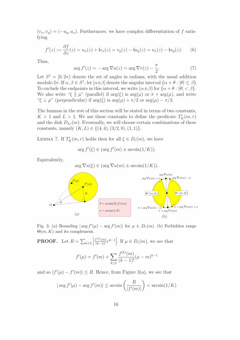
Fig. 3. (a) Bounding | arg f ′(µ) − arg f ′(m)| for µ ∈ Dr(m). (b) Forbidden rangeΘ(m, K) and its complement.

PROOF. Let R =∑

k≥2

∣∣∣f(k)(m)(k−1)!

rk−1∣∣∣. If µ ∈ Dr(m), we see that

f ′(µ) = f ′(m) +∑

k≥2

f (k)(m)

(k − 1)!(µ−m)k−1

and so |f ′(µ)− f ′(m)| ≤ R. Hence, from Figure 3(a), we see that

| arg f ′(µ)− arg f ′(m)| ≤ arcsin

(R

|f ′(m)|

)< arcsin(1/K)

16

since T ′K(m, r) holds implies |f ′(m)| > KR. The equivalent form in terms of

∇u follows from the fact that arg f ′(µ) = − arg∇u(µ).

It follows from this lemma that if T ′K(m, r) holds and µ, ξ ∈ Dr(m) then

|arg f ′(µ)− arg f ′(ξ)| < 2 arcsin(1/K).

Thus, the argument of f ′(z) (for z ∈ Dr(m)) cannot vary by more than2 arcsin(1/K).

The next property is, of course, a generalization of Lemma 1(ii).

Lemma 8. If K ≥√

2 and T ′K(m, r) holds, then the disk Dr(m) has at most

one zero of f .

PROOF. Say a, b are two zeros of f in Dr(m). As a = b implies f ′(a) = 0,which is not possible as T ′

1(m, r) holds, we can assume a 6= b. Then f(a) =f(b) = 0 and so u(a) = v(a) = u(b) = v(b) = 0. But u(a) = u(b) = 0 implies,by the Mean Value Theorem, that there exists µ ∈ [a, b] such that

∇u(µ) ⊥ (b− a).

Similarly, v(a) = v(b) = 0 implies there exists ξ ∈ [a, b] such that

∇v(ξ) ⊥ (b− a).

But ∇v(ξ) = (vx(ξ), vy(ξ)) = (−uy(ξ), ux(ξ)). It follows that

∇u(ξ) ‖ (b− a).

Therefore ∇u(µ) and ∇u(ξ) must be perpendicular.

On the other hand, Lemma 7 says that if µ, ξ ∈ Dr(m), then arg∇u(µ) andarg∇u(ξ) differ by less than 2 arcsin(1/K). Since K ≥

√2, they differ by less

than 2 arcsin(1/√

2) = π/2. This contradicts the perpendicularity betweenarg∇u(µ) and arg∇u(ξ).

4.2 Crossings of u = 0 on Disk Boundary

We next prove several lemmas that show that u-crossings of a disk Dr(m) arequite restricted under the following assumption.

The predicate T ′K(m, r) holds for some K ≥

√2. (8)

A similar argument shows corresponding results for v-crossings. To focus onthe behavior of the function u(z) = u(x, y) on the boundary of Dr(m), it is

17

useful to consider u there as a function of the angle φ

um,r(φ) := u(m+ reiφ). (9)

From our earlier definition, there is a u-crossing of Dr(m) at φ iff um,r(φ) = 0.

We introduce the notation

Θ(m,K) := (arg∇u(m)±arcsin(1/K)) ∪(π+arg∇u(m)±arcsin(1/K)) ⊆ S1

for the double cone of angles. In Figure 3(b), this double cone is indicated bytwo white sectors. We call Θ(m,K) the forbidden range. The complementof the forbidden range is composed of two angular ranges (see Figure 3(b)),

Θ+(m,K) := [arg∇u(m) + π2± arccos(1/K)]

Θ−(m,K) := [arg∇u(m)− π2± arccos(1/K)].

(10)

The “forbidden” terminology is partly motivated by the next lemma. We showthat the derivative u′m,r(φ) := dum,r

dφ(φ) of um,r(φ) does not vanish if φ lies

outside the forbidden range.

Lemma 9. Assume (8).

(i) If u′m,r(φ) = 0 then φ ∈ Θ(m,K).

(ii) There is at most one u-crossing of Dm,r in Θ+(m,K), and at most oneu-crossing of Dm,r in Θ−(m,K).

PROOF. (i) Let µ = m+ reiφ. Note that

u′m,r(φ) :=dum,rdφ

(φ) =ux(m+ reiφ)(−r sinφ) + uy(m+ reiφ)(r cosφ).

Since ei(φ+π/2) = − sinφ+ i cosφ, we conclude that

u′m,r(φ) = 0 ⇔ ∇u(µ) ⊥ ei(φ+π/2)

⇔ ∇u(µ) ‖ ei(φ).(11)

Thus u′m,r(φ) = 0 implies arg∇u(µ) is equal to φ or to π+φ. Since (8) impliesarg∇u(µ) ∈ Θ(m,K), we conclude that φ ∈ Θ(m,K).

(ii) This is an immediate application of part (i) using Rolle’s Theorem.

18

The preceding lemma implies that there are at most two u-crossings outsidethe forbidden range. And in case that there are two such crossings, they mustlie on opposite sides of the circle separated by the forbidden range. The nextlemma is also useful for limiting u-crossings to at most two without consider-ation of the forbidden range.

Lemma 10. Assume (8) and suppose there are three u-crossings of Dr(m) at

φ1, φ2, φ3 ∈ S1. Let ai = m + reiφi . Then each side of the triangle ∆a1a2a3 isshorter than 4r/K.

PROOF. We consider a line segment [ai, aj]. As u(ai) = u(aj) = 0, theMean Value Theorem implies that there exists a point ξij on [ai, aj] where∇u(ξij) ⊥ (aj − ai). Now if an interior angle of the triangle ∆a1a2a3 is inbetween (2 arcsin(1/K), π − 2 arcsin(1/K)), at least for two of the gradients∇u(ξij), their arguments would differ by more than 2 arcsin(1/K). But thiswould contradict Lemma 7. W.l.o.g. let us consider the angle α3 at the pointa3. Then from the extended sine theorem we get |a2 − a1|/ sin(α3) = 2r, thuswe must have |a2−a1| = 2r sin(α3) < 2r sin(2 arcsin(1/K)) < 4r/K. Similarly,|a3 − a1|, |a3 − a2| < 4r/K, too.

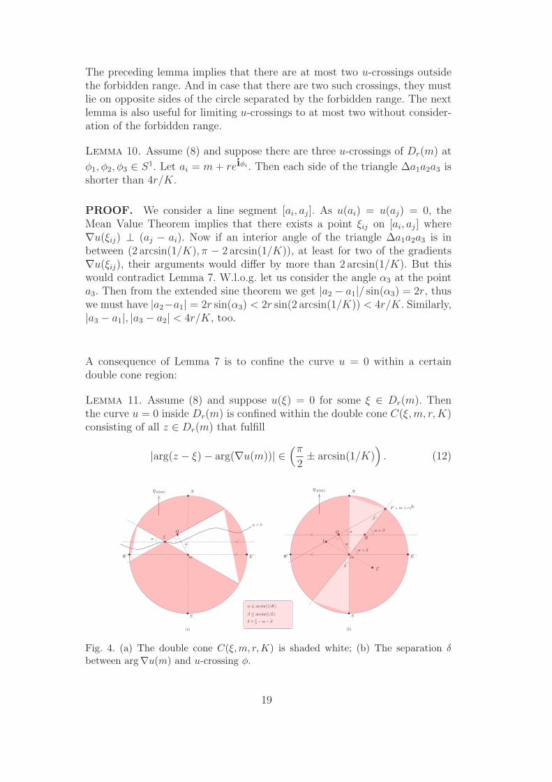
A consequence of Lemma 7 is to confine the curve u = 0 within a certaindouble cone region:

Lemma 11. Assume (8) and suppose u(ξ) = 0 for some ξ ∈ Dr(m). Thenthe curve u = 0 inside Dr(m) is confined within the double cone C(ξ,m, r,K)consisting of all z ∈ Dr(m) that fulfill

|arg(z − ξ)− arg(∇u(m))| ∈(π

2± arcsin(1/K)

). (12)

N

W

β

Q α

W

N

S

Emm E

S

Q

P = m + reiφ

u = 0

∇u(m)∇u(m)

δ = π2 − α− β

α ≤ arcsin(1/K)

β ≤ arcsin(1/L)

δ

ξR

α + β

(b)

αα

α

ξ

ξ′

(a)

α + β

Fig. 4. (a) The double cone C(ξ, m, r, K) is shaded white; (b) The separation δ

between arg∇u(m) and u-crossing φ.

19

PROOF. In Figure 4(a), the angle arg∇u(m) is viewed as pointing north-ward, and the double cone C(ξ,m, r,K) is shaded white. If u(z) = 0 for anyz ∈ Dr(m), then by the Mean Value Theorem, there is a point µ on the linesegment [ξ, z] such that

∇u(µ) ⊥ (z − ξ). (13)

By the previous lemma,

| arg∇u(µ)− arg∇u(m)| ≤ arcsin(1/K). (14)

But (13) and (14) is equivalent to z ∈ C(ξ,m, r,K), as is evident from Fig-ure 4(a).

The next two lemmas show that if the curve u passes relatively close to thecenter of Dr(m) (say, within distance r/L for some L > 1) then the u-crossingsare separated from arg∇u(m) and from the v-crossing. First we show that u-crossings are separated from arg∇u(m), as illustrated in Figure 4(b).

Lemma 12. Assume (8) and ξ is a root of f(z) with |ξ −m| ≤ r/L for someL > 1. Then for any u-crossing φ of Dr(m), it obtains that φ and arg∇u(m)are δ-separated where

δ ≥ δ(K,L) :=π

2− arcsin(1/K)− arcsin(1/L).

Similarly, φ and π+arg∇u(m) are δ-separated. If δ(K,L) > arcsin(1/K) thenu has exactly two u-crossing, one in Θ+(m,K) and the other in Θ−(m,K).

PROOF. Refer to Figure 4(b) where again we assume ∇u(m) is pointingnorthward. Thus, (N − m) ‖ ∇u(m) where N is the north pole of Dr(m)(see Figure 4). If φ lies in the third or fourth quadrants, then clearly φ andarg∇u(m) are δ-separated. Otherwise, by symmetry, we may assume φ lies in

the first quadrant. Let P be the point m+ reiφ. So by assumption, u(P ) = 0.Consider the angle δ := ∠(PmN) (see Figure 4(b)). Thus we must prove thatδ ≥ π

2− arcsin(1/L)− arcsin(1/K).

Consider the line Pm: the point ξ is either above or below the line. It is nothard to see that the minimum value of α(PmN) is attained only if ξ lies abovePm, as seen in Figure 4(b). For instance, the point ξ′ in Figure 4(b) lies belowPm, but it can be replaced by ξ := 2m− ξ which lies symmetrically oppositerelative to center m.

Let Q be the point on the line Pξ that is closest to m. Let R be the pointon the line Pm so that (Q − R) ⊥ ∇u(m). If we define α := ∠(RQP ) andβ := ∠(RPQ) then it easily seen that δ = π

2− α − β. From Lemma 11, we

conclude that α ≤ arcsin(1/K) and from the assumption that |ξ −m| ≤ r/L,

20

we see from examining the triangle ∆(Pξm) that β ≤ arcsin(1/L). These twoinequalities imply

δ ≥ (π/2)− arcsin(1/K)− arcsin(1/L).

By a symmetrical argument, we also conclude that π+∇u(m) and φ must beseparated by an angle of at least ((π/2)− arcsin(1/K)− arcsin(1/L)).

It remains to prove the claim about the number of crossings for δ(K,L) >arcsin(1/K). As Dr(m) contains a root of f the image of ∂Dr(m) under thefunction f is a curve in C that circles the origin at least once, thus we musthave at least two u−crossing on ∂Dr(m). We have already shown that allu−crossings are separated from ∇u(m) and π+∇u(m) by an angle of at leastδ(K,L). Hence, from our definition of the forbidden range it follows that allu−crossings are located outside the forbidden range, thus the claim aboutexactly two u-crossings follows from Lemma 9.

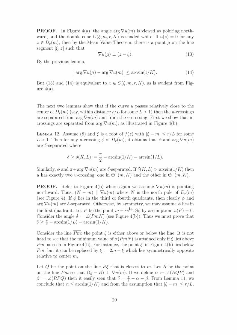
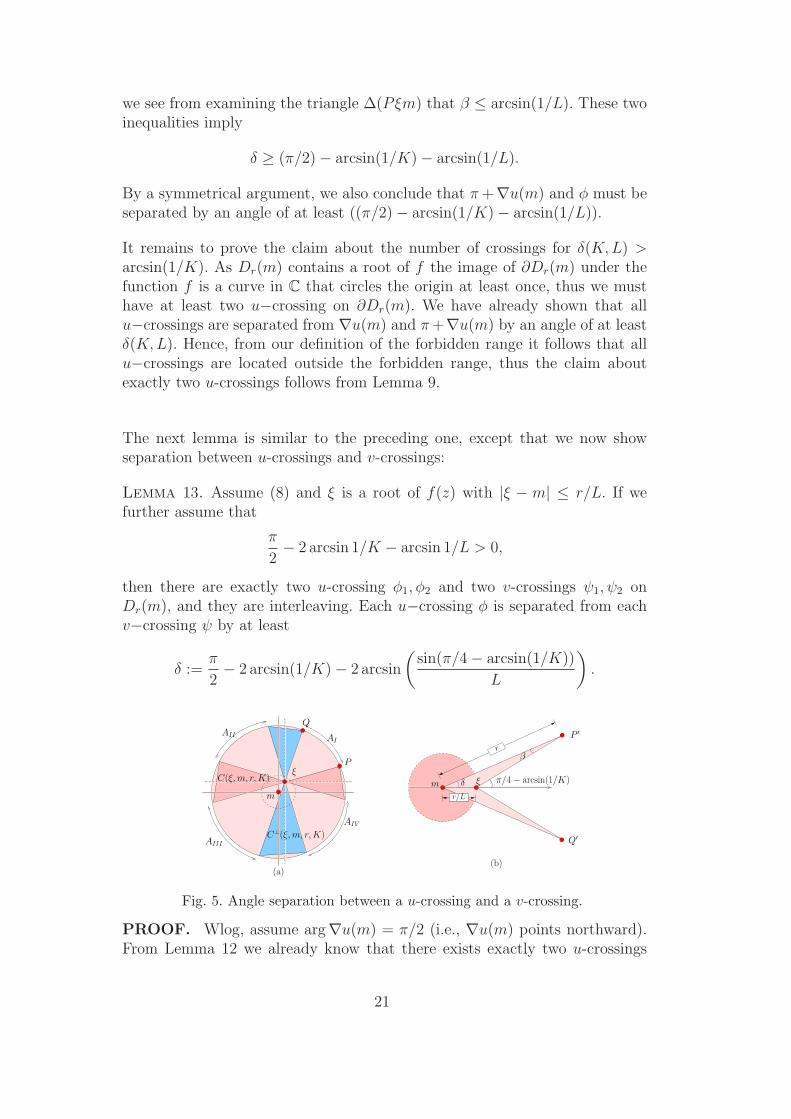
The next lemma is similar to the preceding one, except that we now showseparation between u-crossings and v-crossings:

Lemma 13. Assume (8) and ξ is a root of f(z) with |ξ − m| ≤ r/L. If wefurther assume that

π

2− 2 arcsin 1/K − arcsin 1/L > 0,

then there are exactly two u-crossing φ1, φ2 and two v-crossings ψ1, ψ2 onDr(m), and they are interleaving. Each u−crossing φ is separated from eachv−crossing ψ by at least

δ :=π

2− 2 arcsin(1/K)− 2 arcsin

(sin(π/4− arcsin(1/K))

L

).

ξP

Q

(a)(b)

m

AIAII

AIII

AIV

r/L

r

π/4− arcsin(1/K)

P ′

m δ

Q′

β

ξ

C⊥(ξ,m, r,K)

C(ξ,m, r,K)

Fig. 5. Angle separation between a u-crossing and a v-crossing.

PROOF. Wlog, assume arg∇u(m) = π/2 (i.e., ∇u(m) points northward).From Lemma 12 we already know that there exists exactly two u-crossings

21

φ1, φ2 and two v-crossings ψ1, ψ2. Let φ be a u-crossing, then we have u(P ) = 0

where P = m + reiφ, and likewise v(Q) = 0 where Q = m + reiψ, ψ av−crossing. By Lemma 11, P lies in the cone C(ξ,m, r,K), and similarly,Q lies in the cone C⊥(ξ,m, r,K), defined as the cone C(ξ,m, r,K) rotatedby 90◦ about the point ξ. See Figure 5(a). From the assumption that π

2>

2 arcsin 1/K, it follows that the two cones only share the point ξ. It followsthat the u− and v− crossings are interleaving. The complement of

(∂C(ξ,m, r,K) ∪ ∂C⊥(ξ,m, r,K)

)∩ ∂Dr(m)

is comprised of four arcs AI , AII , AIII , AIV . Because ∇u(m) points northward,arc Ai may be associated with ith quadrant (i ∈ {I, II, III, IV }) in a naturalway. The angle subtended by arc Ai at m is proportional to the arc length ofAi. It is not hard to see that the minimum angle ∠(PmQ) is attained underthe following conditions:(a) P and Q are endpoints of one of these arcs.(b) |m− ξ| = r/L.(c) Measure of angle ∠(PξQ) is (π/2)− 2 arcsin(1/K).

Consider the somewhat more general situation where A′ is any arc of ∂Dr(m)with endpoints P ′ and Q′ satisfying the analogues of conditions (a),(b), and(c). What is the minimum measure of ∠(P ′mQ′)? This measure is minimizedwhen the line mξ bisects the angle ∠(P ′ξQ′). Thus the exterior angle at∠(P ′ξm) has measure that is half of ∠(P ′ξQ′), i.e., (π/4)− arcsin(1/K). Thisoptimal configuration is illustrated in Figure 5(b).

If β is the measure of ∠(mP ′ξ), then the sign formula for ∆(P ′mξ) shows that

sin(β) =sin(π/4− arcsin(1/K))

L

Let δ′ := (π/4) − arcsin(1/K) − β. The lemma follows from the fact thatarg(P ′ −m) and arg(Q′ −m) are 2δ′-separated.

4.3 Application to the 8-Point Test

We are now ready to apply the preceding lemmas, using them to prove Theo-rem 2. Recall that this theorem is concerned with the success and non-successof the 8-Point Test for D4r(m). We now fix the constants K = 6 and L = 4.

We also want to slightly generalize the 8-Point Test by allowing some flexibilityin choosing the 8 main compass points. Given 0 ≤ θ0 < θ1 < · · · < θ7 < 2π,

we can define the 8 main compass points on D4r(m) to be Pi := m + 4reiθi

(i = 0, . . . , 7). Say these compass points are δ-approximate if each pair

22

(θi, θj) is δij-separated where

δij ∈ [45◦ ± δ].

We are interested in an Approximate 8-Point Test based on such a set ofδ-separated compass points. The following is the slightly generalized versionof Theorem 2:

Theorem 14 (Success of Approximate 8-Point Test). Assume the 8-PointTest is based on a set of 2.5◦-separated compass points.

(i) If T ′6(m, 4r) holds and Dr(m) is isolating, then D4r(m) passes the approx-

imate 8-Point Test.

(ii) If T ′6(m, 4r) holds and D4r(m) passes the approximate 8-Point Test, then

D4r(m) is isolating.

PROOF. We first prove the Part (ii). If an approximate 8-Point Test suc-ceeds for D4r(m), then we must show that D4r(m) contains a root of f . By theassumption T ′

6(m, 4r), we know that D4r(m) has at most one root. The suc-cess of the test implies that there are two arcwise u-crossings and two arcwisev-crossings, and these interleave. Thus, there are two u-crossings φ+, φ− thatare 42.5◦-separated. A calculation shows that the distance |P − Q| between

P = m+ 4reiφ+

and Q = m+ 4reiφ−

is at least 4r√

2− 2 cos 42.5◦ ≈ 2.9r

If there are any other u-crossings, then Lemma 10 implies the distance |P −Q|is at most 4(4r)/6 ≈ 2.67r, which is a contradiction. Therefore, the u-curvehas exactly one connected component within D4r(m). Similarly for the v-curve. Since the u-crossings and v-crossings are interleaving, they must inter-sect within D4r(m). This intersection is the root we seek.

We now prove Part (i), so let us assume that Dr(m) contains a root ξ of f .

1. From Lemma 13 we know that there exists exactly two u−crossings φ+, φ−

and two v−crossings ψ+, ψ− which are interleaving.

2. Recall that the main compass points of D4r(m) divides ∂D4r(m) into eightarcs. For any angle φ, let A(φ) denote the arc that contains φ. We claim thatthere is an arc-wise crossings at A(φ∗) where φ∗ is either φ+ or φ−. Since φ∗

is at least π/2 − arcsin(1/4) − arcsin(1/6) ≈ 65◦-separated (see Lemma 12)from arg∇u(m), and arcsin(1/6) ≈ 9.6◦, we conclude that the two endpointsφ1, φ2 of A(φ∗) lie outside Θ(m, 4). This proves that um,4r(φ1)um,4r(φ2) < 0.Moreover, A(φ+) and A(φ−)) are distinct because they are separated by theforbidden range.

3. By the same argument we see exactly two arc-wise intersections at twodistinct arcs A(ψ+) and A(ψ−) for v. As we already know that the u- and v-

23

crossings are interleaving it remains to show that A(ψ∗) and A(φ∗) are distinctfor φ∗ ∈ {φ+, φ−} and ψ∗ ∈ {ψ+, ψ−}. If A(φ∗) = A(ψ∗), then φ∗ and ψ∗ areseparated by at most 50◦. But this contradicts our result in Lemma 13 whichsays that these crossings are separated by at least

π

2− 2 arcsin(1/6)− 2 arcsin

(sin(π/4− arcsin(1/6))

4

)≈ 54.15◦.

This concludes our proof of Theorem 14.

5 Complexity Analysis

This section justifies the lemmas stated in Section 3.7 on the complexity ofCEVAL and EVAL. In particular, we introduce our cluster analysis technique.

5.1 The Clustering Approach

For the complexity analysis we need non-trivial bounds on the quotients

λk := |f (k)(m)||f(m)| where m is the midpoint of a box B in C, as these values

determine the success of our chosen predicates. It is easy to see (see Sec-tion 5.2) that Σk(m) := (

∑i

1|m−zi|)

k constitutes an upper bound on λk(m)where z1, . . . , zn denote the complex roots of f . Thus, before we turn to thecomplexity analysis we formulate a number of useful results to estimate thesum Σ1(m), in particular, we derive non-trivial upper bounds when m is lo-cated outside some “small” neighborhoods of the roots zi.

Let δ > 0, and suppose R ⊆ R is a non-empty multiset of real numbers.Multiset means that elements of R may be duplicated, and its size is denoted|R|, with multiplicity counted. Then its center of gravity is

cg(R) :=

(∑

x∈Rx

)/|R|,

and δ-interval isIδ(R) := (cg(R)± |R|δ).

Thus the width of the Iδ(R) is 2|R|δ.

A ranking of R is a one-one onto function r : R→ {1, 2, . . . , |R|}. We call Ra semi δ-cluster if there is a ranking r of R such that for all x ∈ R,

(cg(R) + |R|δ)− x ≥ r(x)δ. (15)

We call R a δ-cluster if both R and −R = {−x : x ∈ R} are δ-clusters.

24

Rewriting (15) asx− cg(R) ≤ (|R| − r(x))δ

we see that the right-hand side is non-negative, and the inequality is automaticwhen x ≤ cg(R). We are mainly interested in clusters, but it is easier to proveproperties for semi-clusters and to extend them to clusters by symmetry.

Consider the following examples:

Rn = {x1, . . . , xn} ,where x1 = xi for all i;

R1 = {−3, 1, 2} ;

R2 = {x1, x2} ;

R3 = {−x, 0, x} .

Rn is a δ-cluster for any δ > 0. R1 is a semi 1-cluster with cg(R1) = 0, butit is not a 1-cluster. R2 is a δ-cluster iff |x0 − x1| ≤ 2δ. R3 is a δ-cluster iff|x| ≤ 2δ.

5.1.1 Properties of Clusters

The following is immediate:

Lemma 15. If R is a δ-cluster, then R is contained in Iδ(R). In fact, a strongercontainment is true:

R ⊆ [cg(R)± (|R| − 1)δ].

This lemma motivates a useful definition: a collection P = {R1, . . . , Rk} iscalled a δ-partition (of the set R =

⋃ki=1Ri) if each Ri is a δ-cluster and

the intervals Iδ(Ri) are pairwise disjoint. Let Iδ(P) :=⋃ki=1 Iδ(Ri). Clearly, a

δ-partition of R induces an ordinary partition of R.

Another useful property is this:

Lemma 16. If R is a δ-cluster and p /∈ Iδ(R) then

∑

x∈R

1

|p− x| ≤1 + ln |R|

δ.

If P =⋃i=1,...,k Ri is a δ-partition of a multiset R, and p /∈ Iδ(P) then

∑

x∈R

1

|p− x| ≤2(1 + ln ⌈|R|/2⌉)

δ.

PROOF. As p /∈ Iδ(R), then we may, wlog, assume that p > x for all x ∈ R.We only consider the first case as the case p < x can be treated completely

25

similar. If r is the ranking function that witnesses R as a semi δ-cluster thenwe have

∑

x∈R

1

|p− x| ≤|R|∑

i=1

1

|p− r−1(i)| ≤|R|∑

i=1

1

iδ≤ 1 + ln |R|

δ.

For the proof of the second claim we assume, wlog, that the clusters are orderedin way such that x < y for all i < j and x ∈ Ri, y ∈ Rj. Let R0 :=

⋃i=1,...,k0

Ri

be the union of all points x ∈ R with x < p and R1 :=⋃i=k0+1,...,k Ri. Notice

that p separates clusters as it is not contained in any Iδ(Ri). For i ≤ k0 andx ∈ Ri we define the ranking function r : R0 → {1, . . . , |R0|} by r(x) :=∑k0

j=i+1 |Ri|+ ri(x) where ri denotes the ranking function that witnesses Ri asa semi δ-cluster. It follows that |p− x| ≥ r(x)δ ≥ lδ if x is the l-th element ofR0 left to p. Hence, we get

∑

x∈R0

1

|p− x| ≤|R0|∑

l=1

1

|p− r−1(l)| ≤|R0|∑

l=1

1

lδ≤ 1 + ln |R0|

δ.

In an analogous manner we also show∑

x∈R1|p− x|−1 ≤ (1 + ln |R1|)/δ, and

thus ∑

x∈R

1

|p− x| ≤2 + ln |R0|+ ln |R1|

δ≤ 2(1 + ln ⌈|R|/2⌉)

δ.

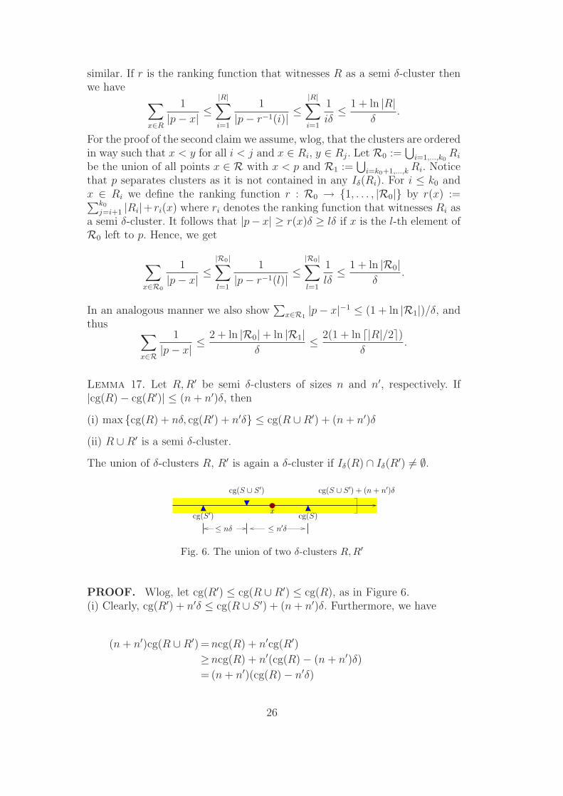
Lemma 17. Let R,R′ be semi δ-clusters of sizes n and n′, respectively. If|cg(R)− cg(R′)| ≤ (n+ n′)δ, then

(i) max {cg(R) + nδ, cg(R′) + n′δ} ≤ cg(R ∪R′) + (n+ n′)δ

(ii) R ∪R′ is a semi δ-cluster.

The union of δ-clusters R, R′ is again a δ-cluster if Iδ(R) ∩ Iδ(R′) 6= ∅.

x

cg(S ∪ S ′) + (n+ n′)δ

cg(S)cg(S ′)

cg(S ∪ S ′)

≤ n′δ≤ nδ

Fig. 6. The union of two δ-clusters R, R′

PROOF. Wlog, let cg(R′) ≤ cg(R ∪R′) ≤ cg(R), as in Figure 6.(i) Clearly, cg(R′) + n′δ ≤ cg(R ∪ S ′) + (n+ n′)δ. Furthermore, we have

(n+ n′)cg(R ∪R′) =ncg(R) + n′cg(R′)

≥ncg(R) + n′(cg(R)− (n+ n′)δ)

= (n+ n′)(cg(R)− n′δ)

26

and thus cg(R ∪R′) ≥ cg(R)− n′δ, which shows the second part of (i).(ii) Let r : R→ {1, . . . , n} and r′ : R′ → {1, . . . , n′} be the ranking functionsthat witness R and R′ as the semi δ-clusters, respectively. We choose a newranking function r : R ∪R′ → {1, . . . , n+ n′} where

r(x) =

r(x) if x ∈ R,n+ r′(x) if x ∈ R′.

If x ∈ R, then we have

cg(R ∪R′) + (n+ n′)δ − x ≥ cg(R) + nδ − x ≥ r(x)δ = r(x)δ

as desired. If x ∈ R′, then we also have

cg(R ∪R′) + (n+ n′)δ − x ≥ (cg(R′) + n′δ − x) + nδ ≥ r(x)δ + nδ = r(x)δ.

From the definition of Iδ(R) and Iδ(R′) it is immediate that |cg(R)−cg(R′)| ≤

(|R|+ |R′|)δ if Iδ(R)∩ Iδ(R′) 6= ∅. Hence R∪R′ is a δ-cluster according to (ii).

Lemma 18. Let R be a multiset that contains n points x1, . . . , xn ∈ R andδ > 0 an arbitrary real value. Then there exists a δ-partition P of R and foreach p /∈ Iδ(P) it holds that

n∑

i=1

1

|p− xi|≤ 2(1 + ln ⌈n/2⌉)

δ.

PROOF. Let P = {R1, . . . , Rk} be a partition of R where each Ri is a δ-cluster. We will keep transforming P until it becomes a δ-partition. We startwith P = {{x1}, . . . , {xn}}. In each step we consider clusters R,R′ ⊂ P withIδ(R) ∩ Iδ(R′) 6= ∅. Their union R ∪R′ is again a δ-cluster due to Lemma 17.We remove R and R′ from P and insert R∪R′. When all the intervals Iδ(R) forR ∈ P are pairwise disjoint, we have the desired δ-partition. The statementabout the bound on the sum

∑kj=1

1|p−xi| follows directly from Lemma 16.

5.1.2 Complex Clusters

We now extend the concept of δ-clusters to a multiset R = {z1, . . . , zn} ofcomplex numbers. Let Re[R] and Im[R] denote the multiset of the real andimaginary part of elements in R. We note that in our application, R is theset of roots of a square-free polynomial and hence R is just an ordinary set.Nevertheless, Re[R] and Im[R] will multisets in general.

According to Lemma 18 there exists a δ-partition{R1, . . . , Rk

Re

}of Re[R].

Similarly, let{R1, . . . , Rk

Im

}denote a δ-partition of Im[R]. Each interval

27

Iδ(Ri) (Iδ(Rj)) defines a vertical (horizontal) stripe (see Figure 7 on page 32)in the complex plane, containing all points z ∈ C with Re(z) ∈ Iδ(Ri) (Im(z) ∈Iδ(Rj)). Their overlapping consists of k := kRe · kIm disjoint boxes which we

denote by B1, . . . , Bk. For any point p /∈ ⋃ki=1Bi, either Re(p) /∈ ⋃k

Rei=1 Iδ(Ri)

or Im(p) /∈ ⋃kImi=1 Iδ(Ri), hence from Lemma 18 we get

∑ni=1

1|p−zi| ≤

2(1+ln⌈n/2⌉)δ

.Furthermore, let ǫ ≥ 0 be an arbitrary positive value and Bǫ

i the box that isobtained by enlarging Bi by ǫ in each direction. If B :=

⋃i=1,...,k Bi, then the

total area covered by the union Bǫ :=⋃B∈B B

ǫ of all these enlarged boxes isupper bounded by

∑

i,j

(w(Iδ(Ri)) + 2ǫ)(w(Iδ(Rj)) + 2ǫ) =∑

i

(w(Iδ(Ri)) + 2ǫ) ·∑

j

(w(Iδ(Rj)) + 2ǫ)

≤ (2nδ + 2nǫ)2 = 4n2(δ + ǫ)2.

where the sum is taken over all i = 1, . . . , kRe ≤ n, j = 1, . . . , kIm ≤ n. Wefix this result.

Theorem 19. Let R be a multiset consisting of n points z1, . . . , zn in thecomplex space and ǫ ≥ 0, δ > 0 arbitrary real values. Then there exist disjointaxes-parallel boxes B1, . . . , Bk ⊂ C, k ≤ n2, with the following properties:

(i) The union B :=⋃i=1,...,k Bi of all boxes cover R.

(ii) Bǫ =⋃i=1,...,k B

ǫi covers an area of less than or equal to 4n2(δ + ǫ)2.

(iii) For each point p /∈ B we have∑n

i=11

|p−zi| ≤2(1+ln⌈n/2⌉)

δ.

We conclude this section with another useful lemma. Again we consider amultiset R, consisting of n complex points z1, . . . , zn. We are interested in apartition of R into multisets that consist of nearby points, only. Let σ(zi) :=minj 6=i |zi−zj| denote the distance of zi to its nearest point in R. Furthermore,for an arbitrary δ > 0, we consider the multiset Rδ that contains exactly thosezi with σ(zi) ≤ δ.

Lemma 20. There exists a partition of Rδ into disjoint multisets R1, . . . , Rk

such that |Ri0 | ≥ 2 for each i0 ∈ {1, . . . , k} and |zi − zj| ≤ |Rδ|δ for allzi, zj ∈ Ri0 .

PROOF. Wlog we can assume that Rδ consists of the points z1, . . . , zl withan l ≤ n. We start with z1 and define R1 := {z1}. We further put all points ziin R1 that satisfy |zi− z1| ≤ δ. Then we proceed with each point in R1 in thesame way. If no further point can be added to R1 we consider the set Rδ\R1

of the remaining points and treat it in exactly the same manner. Finally, weend up with a partition R1, . . . , Rk of R such that for any two points in anyRi0 , their distance is less than or equal to (|Ri0| − 1)δ ≤ |Rδ|δ. Furthermore,

28

each of the multisets Ri must contain at least two points as σ(zi) ≤ δ for alli = 1, . . . , l.

5.2 Analysis of the Subdivision Tree

We show that our algorithm CEVAL, despite its simple predicates, is alsoefficient in a theoretical sense. More precisely, we consider the benchmarkproblem of isolating all complex roots of a degree n polynomial with L bitinteger coefficients. In parallel, also the complexity analysis for its real coun-terpart EVAL is given. We show that both algorithms have complexity boundsthat match (in O sense) those of known exact and practical algorithms for realroot isolation.

5.2.1 Notation

In the following considerations let f ∈ Z[z] be a square-free polynomial of de-gree n ∈ N whose coefficients have at most L bits. The complex roots of f andits derivative f ′ are denoted by z1, . . . , zn and z′1, . . . , z

′n−1, respectively. We

further define σ(zi) := minj 6=i |zi − zj| as the distance of zi to its nearest rootand call σ(zi) the separation of zi. W.lo.g. we assume that the roots are orderedwith respect to their separations, that is, z1 has the smallest and zn the largestseparation. For a given positive value δ let k(δ) be the largest index k such thatσ(zk) ≤ 56n2δ. This apparently strange definition is justified by the results inthe Theorems 22 and 23. We further assume that we start with an initial squarebox B0 (interval), centered at the origin and size s0 := w(B0) = d(B0) = 2L+2.By Cauchy’s bound [44,10], B0 contains all roots of f (real roots in case ofEVAL). T CE and T EV denote the subdivision trees induced by CEVAL andEVAL, respectively. At a certain depth h ∈ N of the subdivision tree all boxes(intervals) B have the same size sh := w(B) = d(B) = 2L+2−h. We denote byδh := 3sh/4 = 3 · 2L−h which is an upper bound on the radius of each of theseboxes (intervals).

5.2.2 Width of T CE and T EV

For a given point m and radius r the success of our exclusion predicate

T fK(m, r) : |f(m)| −K∑

k≥1

∣∣∣∣f (k)(m)

k!rk∣∣∣∣ > 0⇐⇒

∑

k≥1

∣∣∣∣f (k)(m)

f(m)

∣∣∣∣rk

k!< 1/K

29

mainly depends on the quotients∣∣∣f

(k)(m)f(m)

∣∣∣. Each of them can be rewritten as

∣∣∣∣f (k)(m)

f(m)

∣∣∣∣ =

∣∣∣∣∑′

i1,...,ik

1

(m− zi1) . . . (m− zik)

∣∣∣∣ ≤(∑n

i=1

∣∣∣∣1

m− zi

∣∣∣∣)k

where the prime means that the ij’s (j = 1, . . . , k) are chosen to be distinct.In the following we investigate in a good estimation of the sum Σ1(m) :=∑n

i=11

|m−zi| . We start with a simple observation:

Lemma 21. Let δ > 0 be an arbitrary positive real value and |m − zi| ≥ nδfor all i, then T fK(m, r) is true for all K < (e

rδ − 1)−1. In particular,

• T1(m, r) succeeds if |m− zi| > 2nr for all i = 1, . . . , n

• T ′6(m, 4r), T

′3/2(m, 8r) succeed if |m−z′i| > 28(n−1)r for all i = 1, . . . , n−1.

PROOF. From |m− zi| > nδ we get Σ1(m) < 1/δ, thus

∑

k≥1

∣∣∣∣f (k)(m)

f(m)

∣∣∣∣rk

k!<∑

k≥1

1

k!

(rδ

)k< e

rδ − 1 ≤ 1/K.

In particular, for δ := 2r (δ := 28r applied to f ′) as (e1/2 − 1)−1 > 1 ((e1/7 −1)−1 > 6, (e2/7 − 1)−1 > 3/2).

Now let us consider a box of a certain depth h in the subdivision tree. Ifthe midpoint m(B) of such a box B fulfills |m(B) − zi| > 2nδh for all i =1, . . . , n then T1(m(B), δh) succeeds according to the previous lemma, thus Bis omitted. For each root zi, there exist at most O(n2) boxes with |mB − zi| ≤2nδh. Thus, in total, at most O(n3) boxes are retained. This straightforwardobservation is based on a pretty rough estimation of Σ1 which assumes that,from a given point m, the distances to all roots zi have roughly the sameminimal value. In the following, we will use our results from Section 5.1 toshow that this preliminary bound can be substantially improved.

Theorem 22. (Width of T CE) For each h ∈ N, there exist disjoint squareopen axes-parallel boxes B1, . . . , Bk ⊂ C, k ≤ k(δh), such that

(i) The total area of all boxes is at most

(8k(δh)(1 + ln ⌈|k(δh)/2|⌉)δh)2

(ii) For allm ∈ C\⋃ki=lBl either T1(m, δh) or both, T ′

6(m, 4δh) and T ′3/2(m, 8δh)

succeed.

30

(iii) The width wh of T CE at the depth h ∈ N is bounded by

wh < (12k(δh−1)(2 + ln(k(δh−1) + 1)))2 = O(k(δh−1)2 ln k(δh−1)

2)

This result shows that the width of T CE is bounded by O(n2(lnn)2). We nextformulate a version of the above theorem for the real case. It shows that theEVAL algorithm induces a subdivision tree whose width is O(n lnn).

Theorem 23. (Width of T EV ) There exist disjoint open intervals I1, . . . , Ik,k ≤ k(δh), on the real axes such that

(i) The total length of all intervals is smaller than or equal to

8k(δh)(1 + ln ⌈|k(δh)/2|⌉)δh

(ii) For all m ∈ R\⋃kl=1 Il either T1(m, δh) or T ′

1(m, δh) succeeds.

(iii) The width wh of T EV at the depth h ∈ N is bounded by

wh < 3k(δh−1)(5 + ln(k(δh−1) + 1)) = O(k(δh−1) ln k(δh−1)) = O(n lnn).

S2

Re

Im

S1

S1

S2

S3

Root

Projection

z1 = p1 z2 = p2

z4

z3

z5

z6

q4

q3

m

p3 = p4q1 = q2

D6

D5

Root=Projection

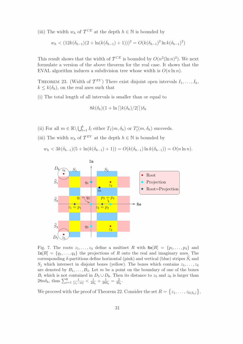
Fig. 7. The roots z1, . . . , z4 define a multiset R with Re[R] = {p1, . . . , p4} andIm[R] = {q1, . . . , q4} the projections of R onto the real and imaginary axes. Thecorresponding δ-partitions define horizontal (pink) and vertical (blue) stripes Si andSj which intersect in disjoint boxes (yellow). The boxes which contains z1, . . . , z4

are denoted by B1, . . . , B4. Let m be a point on the boundary of one of the boxesBi which is not contained in D5 ∪D6. Then its distance to z5 and z6 is larger than28nδh, thus

∑6i=1

1|zi−m| < 1

2δh+ 1

28δh= 2

3δh.

We proceed with the proof of Theorem 22. Consider the setR ={z1, . . . , zk(δh)

},

31

and

δ∗ := 4(1 + ln ⌈k(δh)/2⌉)δh.

We apply Theorem 19 to R, using δ∗ instead of δ and δh instead of ǫ: so thereexist disjoint open axes-parallel boxes B1, . . . , Bk, k ≤ k(δh)

2, such that their

union B :=⋃i=1,...,k Bi has the following properties:

(a) B contains all roots z1, . . . , zk(δh).

(b) Bδh covers an area of at most 4k(δh)2(δh + δ∗)2. Here, Bδh denotes the

union of all boxes in B where we enlarge each Bi by δh in each direction asin 5.1.2.(c) For each point m /∈ B we have

∑k(δh)i=1

1|m−zi| ≤

12δh

.

In the following we only consider those boxes which contain at least one ofthe roots in R. Wlog we can assume that these are the boxes B1, . . . , Bk,where k ≤ k(δh). Obviously the properties (a) and (b) are also fulfilled forB :=

⋃i=1,...,k Bi. Let ∂B :=

⋃i=1,...,k ∂Bi be the union of the boundaries of all

boxes in B, then for each m ∈ ∂B the property in (c) holds, as well.

For the remaining roots zk(δh)+1, . . . , zn, we consider disks Di := D28nδh(zi),i = k(δh) + 1, . . . , n of radius 28nδh, centered at zi. We denote the union ofall these discs by D :=

⋃ni=k(δh)+1Di. Note that D is not necessarily disjoint

from B.

We now prove Part (ii) of Theorem 22. Let m ∈ C be an arbitrary point notcontained in B. We must show that either T1(m, δh) holds, or T ′

6(m, 4δh) andT ′

3/2(m, 8δh) hold. We distinguish two cases:

• m ∈ D: Wlog, we can assume that m ∈ Dn. By definition of k(δh), we haveσ(zn) > 56n2δh. From [10,44] we know that the distance from zn to any rootz′1, . . . , z

′n−1 of f ′ is larger than σ(zn)/n ≥ 56nδh. Thus, the distance from

m to any z′i is larger than 28nδh. According to Lemma 21 the predicatesT ′

6(m, 4δh) as well as T ′3/2(m, 8δh) succeed, thus any box with center m and

radius less than or equal to δh is terminal.

• m /∈ B ∪ D: On C\ (B ∪ D) each quotient f (k)

f, k = 1, . . . , n, defines a

holomorphic function. For each of these functions we have limz→∞f (k)

f(z) =

0. Thus, according to the maximum principle, their maxima are either takenon the boundary of B or on the boundary ∂D of D. Thus, in order to

bound∣∣∣f

(k)

f(m)

∣∣∣, we can restrict to these cases. If m ∈ ∂Di for one of

the discs Di then m is at least 28nδh away from all roots of f and thus∣∣∣f(k)

f(m)

∣∣∣ ≤(∑n

i=11

28nδh

)k=(

128δh

)k. It remains to discuss the case where

m is on the boundary of one of the boxes. Then (c) holds and, in addition,|m− zi| ≥ 28nδh for all i = k(δh) + 1, . . . , n. It follows that

32

∣∣∣∣f (k)

f(m)

∣∣∣∣ ≤(∑k(δh)

i=1

1

|zi −m|+∑n

i=k(δh)+1

1

|zi −m|

)k

≤(

1

2δh+ (n− k(δh)) ·

1

28nδh

)k<

(2

3δh

)k.

Hence, in both situations we have∣∣∣f

(k)

f(m)

∣∣∣ <(

23δh

)kand thus

n∑

k=1

∣∣∣∣f (k)(m)

f(m)

∣∣∣∣δkhk!< e2/3 − 1 < 1.

Hence, T1(m, δh) succeeds and any box with center m and radius smallerthan δh is terminal.

It remains to show (iii) about the number of boxes in Theorem 22. If themidpoint m(B) of a box B of depth h is contained in B then B is completelycontained in Bδh . Bδh covers an area of at most 4k(δh)

2(δh+δ∗) = (2k(δh)δh(5+

4 ln ⌈k(δh/2)⌉))2. As all boxes B at depth h are pairwise disjoint and cover anarea of at least ((4/3)δh)

2 it follows that at most

(3

2k(δh)(5 + 4 ln ⌈k(δh/2)⌉))2 < (6k(δh)(2 + ln(k(δh) + 1)))2

boxes are retained. As each non-terminal node has four children the width whof T CE at height h is bounded by

(12k(δh−1)(2 + ln(k(δh−1) + 1)))2 = O(n2(lnn)2).

The proof of Theorem 23 is a direct consequence of our above considera-tions. Consider the intersection of B with the real axes. The overlapping con-sists of at most k(δh) intervals I1, . . . , Ik and the total length of their unionI :=

⋃l=1,...,k Il is bounded by 2k(δh)δ

∗ = 8k(δh)(1 + ln ⌈k(δh/2)⌉)δh. We havealready shown that for all points m outside these intervals either T1(m, δh)or T ′

6(m, 4δh) succeeds. Then trivially, either T1(m, δh) or T ′1(m, δh) succeeds,

as well. Hence, an interval I of length at most 2δh with midpoint m /∈ I isterminal. If an interval I with midpoint m(I) ∈ I has length at most 2δh,then it is completely contained in Iδh :=

⋃l=1,...,k I

δhl , where Iδhl is obtained by

enlarging Il by δh in both sides. Thus Iδh has total length less than or equalto

2k(δh)(δh + δ∗) < 2k(δh)δh(5− ln 2 + ln(k(δh) + 1)).

At depth h all intervals have width 43δh, thus at most 3

2k(δh)(5−ln 2+ln(k(δh)+

1)) intervals are not terminal. As each non-terminal node in T EV has twochildren the width of T EV at depth h is bounded by 3k(δh−1)(5+ ln(k(δh−1)+1)).

33

5.2.3 Size of T CE and T EV

The preceding analysis gives the width of the trees T CE and T EV . We nowbound their sizes. In particular, our result shows that the subdivision treeinduced by the EVAL algorithm is, at least in terms of O-complexity, as goodas that of well-known methods for real root isolation using Descartes’ Rule ofSign or Sturm sequences.

Theorem 24. For a square-free polynomial f of degree n with coefficients ofat most L bits, the size of T CE is O((n lnn)2(L+ lnn)) = O(n2L). For T EV ,

the size is O(n(L+ lnn)(lnL+ lnn)) = O(nL).

PROOF. We first investigate in a bound on k(δh). As in the proof of Theo-rem 22, consider the set R consisting of those roots z1, . . . , zk(δh) with separa-tion σ(zi) ≤ 56n2δh. Then according to Lemma 20, there exists a partition ofR into disjoints sets R1, . . . , Rk such that |Ri0 | ≥ 2 for each i0 = 1, . . . , n and|zi−zj| ≤ 56n2δh|R| ≤ 56n3δh for all pairs zi, zj ∈ Ri0 . We consider a directedgraph Gi on Ri which connects consecutive points of Ri in ascending order oftheir absolute values. We define G := (R,E) as the union of all Gi. Then G isa directed graph on R with the following properties:

(1) each edge (α, β) ∈ E satisfies |α| ≤ |β|,(2) G is acyclic, and(3) the in-degree of any node is at most 1.

Hence, we can apply the generalized Davenport-Mahler bound [9,10] on G:

∏

(α,β)∈E|α− β| ≥ 1

((n+ 1)1/22L)n−1·(√

3

n

)#E

·(

1

n

)n/2

As each set Ri contains at least 2 roots, we must have #E ≥ k(δh)/2. Fur-thermore, for each edge (α, β) ∈ E we have |α− β| ≤ 56n3δh = 168n32L−h. Itfollows that

(168n32L−h

) k(δh)

2 ≥ 1

((n+ 1)1/22L)n−1·(√

3

n

)k(δh)

·(

1

n

)n/2

>1

(n+ 1)n2nL·(

3

n2

)k(δh)/2

and thus

k(δh) · (5 + 5 lnn+ (L− h) ln 2) > −2n(L ln 2 + ln(n+ 1))

where we used the inequality ln 56 < 5. Thus, for h > L + 8(1 + lnn) >

34

L+ 5ln 2

+ 5 lnnln 2

, we get

k(δh) <2n(L ln 2 + ln(n+ 1))

(h− L) ln 2− 5− 5 lnn<

3n(L+ ln(n+ 1))

h− L . (16)

Since h > L + 8(1 + lnn), we may define h′ := h − h0 ∈ N where h0 :=⌈L+ 8(1 + lnn)⌉. Then (16) transforms into

k(δh) <3n(L+ ln(n+ 1))

h′ + ⌈8(1 + lnn)⌉ <3n(L+ ln(n+ 1))

h′. (17)

For all h ≤ 2h0 we use the simple inequality k(δh) ≤ n whereas for h > 2h0

we use the bound on k(δ) in (17). From (17), we can bound on the heighthmax of TCE as follows. Observe by Theorem 22(iii) that when k(δh) = 0then the width is 0. So we may assume k(δh) ≥ 1 in (17). Therefore h′ ≤3n(L+ ln(n+ 1)). Therefore

hmax ≤ h′ + h0 ≤ 3n(L+ ln(n+ 1)) + L+ 8(1 + lnn) = O(n(L+ lnn)).

Now we are able to compute the size of TCE:

∣∣TCE∣∣ ≤

hmax∑

h=1

(12k(δh−1)(2 + ln(k(δh−1) + 1)))2 (by Theorem 22)

≤ 144

2h0∑

h=1

(n(ln(n+ 1) + 2))2 + 144

hmax−h0∑

h′=h0+1

9n2

(L+ ln(n+ 1)

h′

)2

· (2 + ln(n+ 1))2

= O(n2(lnn)3 + L(n lnn)2) +O(n2(L+ lnn)2) · (2 + ln(n+ 1))2 ·hmax−h0∑

h′=h0+1

(1

h′

)2

= O(n2(lnn)3 + L(n lnn)2) +O(n2(L+ lnn)2) · (2 + ln(n+ 1))2 · 1

L+ lnn

= O((n lnn)2(L+ lnn)) = O(n2L).

For the size of TEV we obtain

∣∣TEV∣∣ ≤

hmax∑

h=1

3k(δh−1)(5 + ln(k(δh−1) + 1))

(by Theorem 23)

≤ 3

h0∑

h=1

n(ln(n+ 1) + 5) + 9(5 + ln(n+ 1)) ·hmax−h0∑

h′=1

nL+ ln(n+ 1)

h′

= O(n lnn(L+ lnn)) +O(n(L+ lnn) lnhmax lnn)

= O(n(L+ lnn)(lnL+ lnn) = O(nL).

35

5.3 Bit Complexity

We will see that the larger tree size of TCE does not lead to an asymptoticallylarger bit complexity when compared to TEV . More precisely, both algorithmsuse O(n4L2) bit operations to isolate the roots of f (either real or complex).

Theorem 25. For a square-free polynomial f of degree n with integer coeffi-cients of at most L bits, CEVAL and EVAL isolate the complex (real) roots

of f with a number ∆CE (∆EV ) of bit operations bounded by O(n4L2).

PROOF. We refer to Section 6 where we show that, for each node v of TCE

(TEV ) of depth h, the number λv of bit operations is bounded by O(nL+n2h).

For all h ≤ 2h0 = 2 ⌈L+ 8(1 + lnn)⌉ = O(L) this simplifies to λv = O(n2L).Now our claim about the bit complexity derives from a simple computation(cf. proof of Theorem 24):

∆CE ≤2h0∑

h=1

(n(ln(n+ 1) + 2))2O(n2L)

+

hmax−h0∑

h′=h0+1

n2

(L+ ln(n+ 1)

h′

)2

O(nL+ n2(h′ + h0))

= O(n4L2) +

hmax−h0∑

h′=h0+1

n4

(L+ ln(n+ 1)

h′

)2

O(h′)

= O(n4L2)(1 +

hmax−h0∑

h′=h0+1

1

h′) = O(n4L2). (18)

In the above inequality (18), we use O(nL + n2(h′ + h0)) = O(n2h′) becausethe second summation is only summed over h′ ≥ h0 > L.For the EVAL algorithm, the computation turns out to be a little simpler,although the final bound is the same:

∆EV ≤h0∑

h=1

n(ln(n+ 1) + 5)O(nL+ n2L)

+

hmax−h0∑

h′=1

nL+ ln(n+ 1)

h′O(nL+ n2(h′ + h0))

= O(n3L2) + O(n3L2)

hmax−h0∑

h′=1

1

h′+ O(n3L)

hmax−h0∑

h′=1

1

h′O(h′) = O(n4L2)

36

6 Exactness and Other Implementation Issues

Our CEVAL algorithm is meant to be practical and suitable for exact imple-mentation. In this section, we address the exactness question and also sometechniques to improve the practical efficiency of CEVAL.

The basis for all our numerical computation is the set of BigFloats or dyadicnumbers, F = {m2n : m,n ∈ Z} = Z[1

2]. The ring operations (+,−,×) are

exact in F, as is division by 2. But general division will be approximated. See[45] for discussion of the use of F for general real computation. In this paper, weuse the obvious extension to complex dyadic numbers F[i]. All input numberswill be assumed to be dyadic; in particular, the polynomial f has coefficientsin F[i], and the initial box B0 = Box(µ, ξ) where µ, ξ ∈ F[i]. Subsequentsubdivision boxes remain dyadic.

Note that m is dyadic, but the exact radius r of the box is not. But we canreplace r by any dyadic upper bound: for square boxes of width w, we mayuse the dyadic value 3/4w for r.

Next we consider the 8 compass points: the cardinal points (N,S,E,W ) aredyadic, but the ordinal points (NE,SE, SW,NW ) are not. In fact, dyadicpoints are generally impossible, and we must settle for some choice of rationalpoints. The proof on the exactness of our algorithm (cf. Theorem 14 in Ap-pendix 4.1) shows that it is sufficient to choose a set of 8 angles {θi : i = 0, . . . , 7}that are pairwise separated by angles in the range [45◦ ± δ] such that each θiis Pythagorean, i.e., sin(θi) and cos(θi) are rational values. It is well knownthat such angles are obtained from Pythagorean triples (x, y, z) ∈ N

3 wherex2 + y2 = z2, and it is also easy to generate such triples.

The amount of deviation δ depends on the choice of some constants K and L— we have not tried to optimize this choice. In Theorem 14, we show that if(K,L) = (6, 4) then we can choose δ = 2.5◦. For our purposes, we only need toapproximate the ordinal points. A useful Pythagorean triple for this purposeis (x, y, z) = (20, 21, 29) Note that arcsin(20/29) ≈ 43.60◦.

In the 8-Point Test, it is not necessary to compute u(x, y) and v(x, y) sepa-rately. Instead, we simply evaluate the function f(z) at the compass pointsP . Note that P will be rational, not dyadic. The signs u(P ) := Re(f(P )) andv(P ) := Im(f(P )) can usually be obtained exactly by interval arithmetic; evenexact sign can be obtained by sufficiently high accuracy approximation andusing zero bounds.

Our main predicates are based on the explicit representation of fB(z) :=f(z +m(B)), the Taylor expansion of f at the center m(B) of a box B. Thedirect computation of fB from f at each node of the recursion is costly. Itis better to compute fB incrementally as follows: let B′ be (wlog) the upper

37

right child of B. We may also assume that our initial box is a square of width2−k (k ∈ Z), centered at a dyadic point. Recursively, B is also a square of thisform. So

f(m(B′)+ z) = f(m(B)+2−k−2(1+ i)+ z) = f(m(B)+2−k−2(2k+2z+1+ i)).

We now compute fB′ from f0(z) := fB(z) in three steps: First scale the func-tion f0 by the substitution z 7→ 2−k−2z to obtain f1(z) := f0(2

−k−2z). Nextapply a Taylor shift by 1, and a shift by i, to get f2(z) := f1(z+1+ i). Finally,we scale again with z 7→ 2k+2z to yield our goal, fB′(z) = f2(2

k+2z).

Assume the standard encoding of binary floating point numbers, each scalingz 7→ 2kz amounts to adding k to the exponents of the polynomial coefficients.Thus the computational cost is dominated by the Taylor shifts. A Taylor shiftby i can be realized as a Taylor shift by 1 combined with two scalings by i, animmediate consequence of the identity f(z+i) = f(i(−iz+1)). Using classical

Taylor shift [17], a shift by 1 requires O(n2(n+ τB)) bit operations, where thecoefficients of fB are represented by 2τB -bit dyadic numbers. However, usingasymptotically fast Taylor shift [14,10], this number reduces to O(n(n+ τB)).Also, the bit complexity of the coefficients grow by O(n) bits in every node.As we start with a polynomial f with integer coefficients of at most L bits,we get τB = O(L+ nh) for each box B at depth h in the subdivision tree.For the predicate evaluations and the point evaluations in the 8-Point Test wehave to compute the value of a polynomial, whose coefficients are O(L+ nh)-bit dyadic numbers, at a point of bit complexity O(1). Therefore O(L+nh) bitoperations are sufficient. It follows that the overall number of bit operationsat a node of depth h is bounded by O(n(n+ τB)) = O(n(L+ nh)).

Our description of the test TK does not exploit any additional informationthat might be obtained while doing the test. For instance, in practice, the testTK(m, r) proceeds by computing the remainder term

R(m, r) :=∑

k≥1

∣∣∣∣f (k)(m)

k!

∣∣∣∣ rk

and |f(m)| separately. Then the test TK(m, r) amounts to checking if |f(m)| >K · R(m, r). Even in the case of a failure, the values |f(m)| and R(m, r) canbe used to determine subsequent actions. In the case of the exclusion testT1(m, r), a success currently excludes the box contained in Dr(m); but infact, the computed value may justify the exclusion of a much larger region.Furthermore, from the Taylor expansion at m we can also derive approximateinformation (via root bounds) about the largest r that fulfills |f(m)| > R(m, r)which allows us to exclude disc regions of a certain size and thus to approxi-mate the roots faster than by simple bisection. But to exploit this, we need toleave the comfortable framework of quadtrees. In future work, we will explore

38

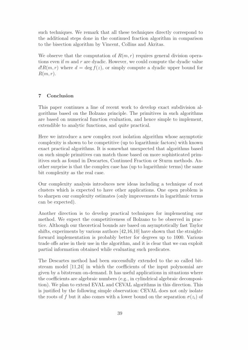
such techniques. We remark that all these techniques directly correspond tothe additional steps done in the continued fraction algorithm in comparisonto the bisection algorithm by Vincent, Collins and Akritas.

We observe that the computation of R(m, r) requires general division opera-tions even if m and r are dyadic. However, we could compute the dyadic valued!R(m, r) where d = deg f(z), or simply compute a dyadic upper bound forR(m, r).

7 Conclusion

This paper continues a line of recent work to develop exact subdivision al-gorithms based on the Bolzano principle. The primitives in such algorithmsare based on numerical function evaluation, and hence simple to implement,extendible to analytic functions, and quite practical.

Here we introduce a new complex root isolation algorithm whose asymptoticcomplexity is shown to be competitive (up to logarithmic factors) with knownexact practical algorithms. It is somewhat unexpected that algorithms basedon such simple primitives can match those based on more sophisticated prim-itives such as found in Descartes, Continued Fraction or Sturm methods. An-other surprise is that the complex case has (up to logarithmic terms) the samebit complexity as the real case.

Our complexity analysis introduces new ideas including a technique of rootclusters which is expected to have other applications. One open problem isto sharpen our complexity estimates (only improvements in logarithmic termscan be expected).

Another direction is to develop practical techniques for implementing ourmethod. We expect the competitiveness of Bolzano to be observed in prac-tice. Although our theoretical bounds are based on asymptotically fast Taylorshifts, experiments by various authors [42,16,10] have shown that the straight-forward implementation is probably better for degrees up to 1000. Varioustrade offs arise in their use in the algorithm, and it is clear that we can exploitpartial information obtained while evaluating such predicates.

The Descartes method had been successfully extended to the so called bit-stream model [11,24] in which the coefficients of the input polynomial aregiven by a bitstream on-demand. It has useful applications in situations wherethe coefficients are algebraic numbers (e.g., in cylindrical algebraic decomposi-tion). We plan to extend EVAL and CEVAL algorithms in this direction. Thisis justified by the following simple observation: CEVAL does not only isolatethe roots of f but it also comes with a lower bound on the separation σ(zi) of

39

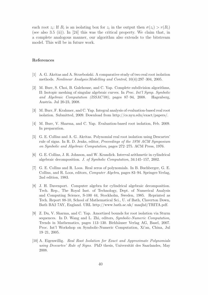
each root zi: If Bi is an isolating box for zi in the output then σ(zi) > r(Bi)(see also 3.5 (ii)). In [24] this was the critical property. We claim that, ina complete analogous manner, our algorithm also extends to the bitstreammodel. This will be in future work.

References

[1] A. G. Akritas and A. Strzebonski. A comparative study of two real root isolationmethods. Nonlinear Analysis:Modelling and Control, 10(4):297–304, 2005.

[2] M. Burr, S. Choi, B. Galehouse, and C. Yap. Complete subdivision algorithms,II: Isotopic meshing of singular algebraic curves. In Proc. Int’l Symp. Symbolicand Algebraic Computation (ISSAC’08), pages 87–94, 2008. Hagenberg,Austria. Jul 20-23, 2008.

[3] M. Burr, F. Krahmer, and C. Yap. Integral analysis of evaluation-based real rootisolation. Submitted, 2009. Download from http://cs.nyu.edu/exact/papers/.

[4] M. Burr, V. Sharma, and C. Yap. Evaluation-based root isolation, Feb. 2009.In preparation.

[5] G. E. Collins and A. G. Akritas. Polynomial real root isolation using Descartes’rule of signs. In R. D. Jenks, editor, Proceedings of the 1976 ACM Symposiumon Symbolic and Algebraic Computation, pages 272–275. ACM Press, 1976.

[6] G. E. Collins, J. R. Johnson, and W. Krandick. Interval arithmetic in cylindricalalgebraic decomposition. J. of Symbolic Computation, 34:145–157, 2002.

[7] G. E. Collins and R. Loos. Real zeros of polynomials. In B. Buchberger, G. E.Collins, and R. Loos, editors, Computer Algebra, pages 83–94. Springer-Verlag,2nd edition, 1983.

[8] J. H. Davenport. Computer algebra for cylindrical algebraic decomposition.Tech. Rep., The Royal Inst. of Technology, Dept. of Numerical Analysisand Computing Science, S-100 44, Stockholm, Sweden, 1985. Reprinted asTech. Report 88-10, School of Mathematical Sci., U. of Bath, Claverton Down,Bath BA2 7AY, England. URL http://www.bath.ac.uk/ masjhd/TRITA.pdf.

[9] Z. Du, V. Sharma, and C. Yap. Amortized bounds for root isolation via Sturmsequences. In D. Wang and L. Zhi, editors, Symbolic-Numeric Computation,Trends in Mathematics, pages 113–130. Birkhauser Verlag AG, Basel, 2007.Proc. Int’l Workshop on Symbolic-Numeric Computation, Xi’an, China, Jul19–21, 2005.

[10] A. Eigenwillig. Real Root Isolation for Exact and Approximate Polynomialsusing Descartes’ Rule of Signs. PhD thesis, Universitat des Saarlandes, May2008.

40

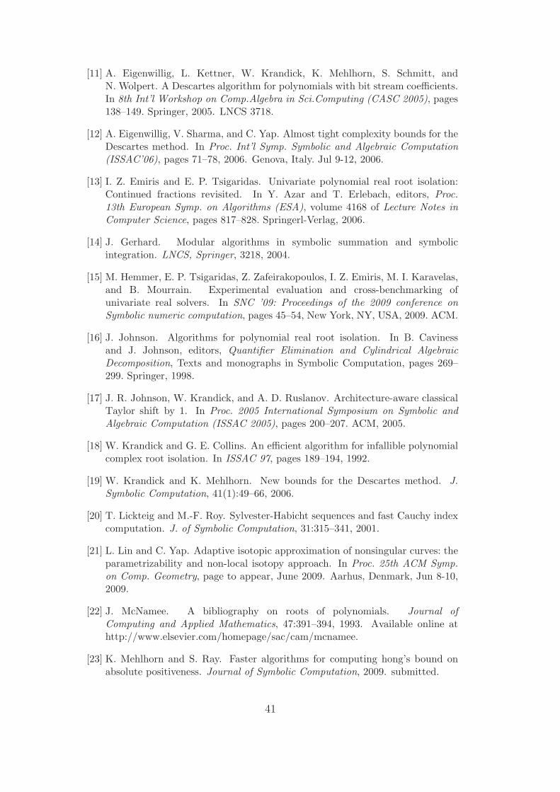
[11] A. Eigenwillig, L. Kettner, W. Krandick, K. Mehlhorn, S. Schmitt, andN. Wolpert. A Descartes algorithm for polynomials with bit stream coefficients.In 8th Int’l Workshop on Comp.Algebra in Sci.Computing (CASC 2005), pages138–149. Springer, 2005. LNCS 3718.

[12] A. Eigenwillig, V. Sharma, and C. Yap. Almost tight complexity bounds for theDescartes method. In Proc. Int’l Symp. Symbolic and Algebraic Computation(ISSAC’06), pages 71–78, 2006. Genova, Italy. Jul 9-12, 2006.

[13] I. Z. Emiris and E. P. Tsigaridas. Univariate polynomial real root isolation:Continued fractions revisited. In Y. Azar and T. Erlebach, editors, Proc.13th European Symp. on Algorithms (ESA), volume 4168 of Lecture Notes inComputer Science, pages 817–828. Springerl-Verlag, 2006.

[14] J. Gerhard. Modular algorithms in symbolic summation and symbolicintegration. LNCS, Springer, 3218, 2004.

[15] M. Hemmer, E. P. Tsigaridas, Z. Zafeirakopoulos, I. Z. Emiris, M. I. Karavelas,and B. Mourrain. Experimental evaluation and cross-benchmarking ofunivariate real solvers. In SNC ’09: Proceedings of the 2009 conference onSymbolic numeric computation, pages 45–54, New York, NY, USA, 2009. ACM.

[16] J. Johnson. Algorithms for polynomial real root isolation. In B. Cavinessand J. Johnson, editors, Quantifier Elimination and Cylindrical AlgebraicDecomposition, Texts and monographs in Symbolic Computation, pages 269–299. Springer, 1998.

[17] J. R. Johnson, W. Krandick, and A. D. Ruslanov. Architecture-aware classicalTaylor shift by 1. In Proc. 2005 International Symposium on Symbolic andAlgebraic Computation (ISSAC 2005), pages 200–207. ACM, 2005.

[18] W. Krandick and G. E. Collins. An efficient algorithm for infallible polynomialcomplex root isolation. In ISSAC 97, pages 189–194, 1992.

[19] W. Krandick and K. Mehlhorn. New bounds for the Descartes method. J.Symbolic Computation, 41(1):49–66, 2006.

[20] T. Lickteig and M.-F. Roy. Sylvester-Habicht sequences and fast Cauchy indexcomputation. J. of Symbolic Computation, 31:315–341, 2001.

[21] L. Lin and C. Yap. Adaptive isotopic approximation of nonsingular curves: theparametrizability and non-local isotopy approach. In Proc. 25th ACM Symp.on Comp. Geometry, page to appear, June 2009. Aarhus, Denmark, Jun 8-10,2009.

[22] J. McNamee. A bibliography on roots of polynomials. Journal ofComputing and Applied Mathematics, 47:391–394, 1993. Available online athttp://www.elsevier.com/homepage/sac/cam/mcnamee.

[23] K. Mehlhorn and S. Ray. Faster algorithms for computing hong’s bound onabsolute positiveness. Journal of Symbolic Computation, 2009. submitted.

41

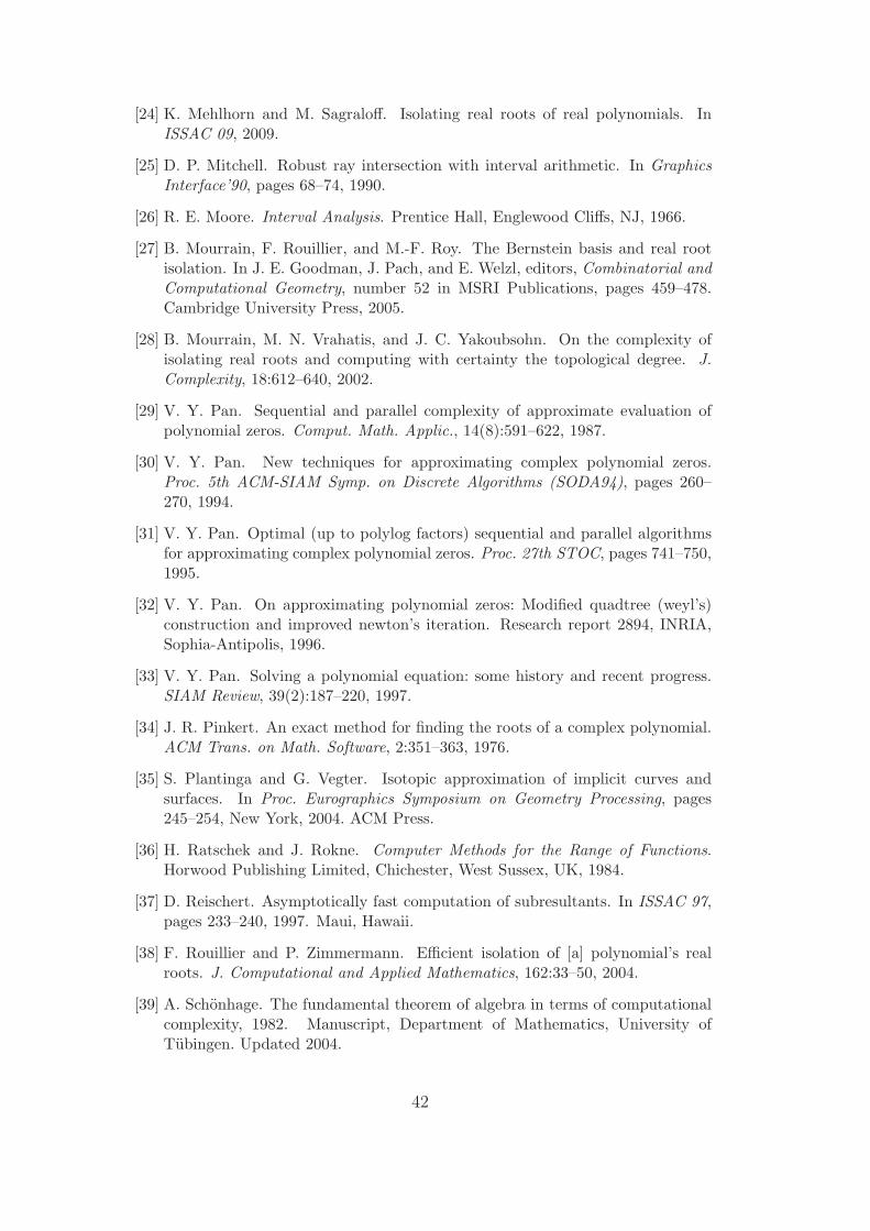
[24] K. Mehlhorn and M. Sagraloff. Isolating real roots of real polynomials. InISSAC 09, 2009.

[25] D. P. Mitchell. Robust ray intersection with interval arithmetic. In GraphicsInterface’90, pages 68–74, 1990.

[26] R. E. Moore. Interval Analysis. Prentice Hall, Englewood Cliffs, NJ, 1966.

[27] B. Mourrain, F. Rouillier, and M.-F. Roy. The Bernstein basis and real rootisolation. In J. E. Goodman, J. Pach, and E. Welzl, editors, Combinatorial andComputational Geometry, number 52 in MSRI Publications, pages 459–478.Cambridge University Press, 2005.

[28] B. Mourrain, M. N. Vrahatis, and J. C. Yakoubsohn. On the complexity ofisolating real roots and computing with certainty the topological degree. J.Complexity, 18:612–640, 2002.

[29] V. Y. Pan. Sequential and parallel complexity of approximate evaluation ofpolynomial zeros. Comput. Math. Applic., 14(8):591–622, 1987.

[30] V. Y. Pan. New techniques for approximating complex polynomial zeros.Proc. 5th ACM-SIAM Symp. on Discrete Algorithms (SODA94), pages 260–270, 1994.

[31] V. Y. Pan. Optimal (up to polylog factors) sequential and parallel algorithmsfor approximating complex polynomial zeros. Proc. 27th STOC, pages 741–750,1995.

[32] V. Y. Pan. On approximating polynomial zeros: Modified quadtree (weyl’s)construction and improved newton’s iteration. Research report 2894, INRIA,Sophia-Antipolis, 1996.

[33] V. Y. Pan. Solving a polynomial equation: some history and recent progress.SIAM Review, 39(2):187–220, 1997.

[34] J. R. Pinkert. An exact method for finding the roots of a complex polynomial.ACM Trans. on Math. Software, 2:351–363, 1976.

[35] S. Plantinga and G. Vegter. Isotopic approximation of implicit curves andsurfaces. In Proc. Eurographics Symposium on Geometry Processing, pages245–254, New York, 2004. ACM Press.

[36] H. Ratschek and J. Rokne. Computer Methods for the Range of Functions.Horwood Publishing Limited, Chichester, West Sussex, UK, 1984.

[37] D. Reischert. Asymptotically fast computation of subresultants. In ISSAC 97,pages 233–240, 1997. Maui, Hawaii.

[38] F. Rouillier and P. Zimmermann. Efficient isolation of [a] polynomial’s realroots. J. Computational and Applied Mathematics, 162:33–50, 2004.

[39] A. Schonhage. The fundamental theorem of algebra in terms of computationalcomplexity, 1982. Manuscript, Department of Mathematics, University ofTubingen. Updated 2004.

42

[40] V. Sharma. Complexity of real root isolation using continued fractions. Theor.Computer Science, 409(2), 2008. Also: proceedings ISSAC’07.

[41] S. Smale. The fundamental theorem of algebra and complexity theory. Bulletin(N.S.) of the AMS, 4(1):1–36, 1981.

[42] J. von zur Gathen and J. Gerhard. Fast algorithms for Taylor shifts and certaindifference equations. In Proc. 1997 International Symposium on Symbolic andAlgebraic Computation (ISSAC 1997), pages 40–47. ACM, 1997.

[43] H. S. Wilf. A global bisection algorithm for computing the zeros of polynomialsin the complex plane. J. of the ACM, 25(3):415–420, 1978.

[44] C. K. Yap. Fundamental Problems of Algorithmic Algebra. Oxford UniversityPress, 2000.

[45] C. K. Yap. Theory of real computation according to EGC. In P. Hertling,C. Hoffmann, W. Luther, and N.Revol, editors, Reliable Implementation of RealNumber Algorithms: Theory and Practice, number 5045 in Lecture Notes inComputer Science, pages 193–237. Springer, 2008.

43